SWEpy: an open-source GPU-accelerated solver for near-field inundation and far-field tsunami modeling

We present SWEpy, an open-source Python finite volume (FV) software for solving the shallow water equations (SWEs) on unstructured triangular meshes. The framework combines flexibility and high performance through GPU acceleration and a well-balanced, positivity-preserving, higher-order central-upwind (CU) scheme. These features are required for simulation of hydrodynamic phenomena such as tsunami propagation, flooding, and dam-break flows in complex and large geometries.

To reduce numerical diffusion, a phenomenon commonly encountered in FV methods, SWEpy incorporates a second-order WENO reconstruction together with a third-order strong stability-preserving Runge–Kutta time integration scheme. These numerical components are particularly well-suited for far-field tsunami modeling, where minimizing artificial diffusion is essential to accurately preserve wave amplitude, phase, and dispersion over long propagation distances.

The performance, stability, and accuracy of SWEpy are validated using canonical benchmarks, including Synolakis’ conical island and Bryson’s flow over a Gaussian bump. Its capabilities are further demonstrated through large-scale simulations of the 1959 Malpasset Dam failure and the 2010 Maule tsunami, highlighting its effectiveness in realistic scenarios. Overall, these results show that SWEpy framework delivers high-resolution solutions on consumer-grade hardware, providing a user-friendly and computationally efficient platform for both research applications and operational forecasting.

1 Introduction

Accurate simulation of hazardous hydrological events – such as dam failures, tsunamis, and urban flooding – is essential for risk assessment, emergency planning, and the operation of early warning systems (Catalan et al., 2020; Fernández-Nóvoa et al., 2024; Lin et al., 2015; Behrens et al., 2010; Harig et al., 2019). Accordingly, over the past three decades, a wide range of numerical tools has been developed for these applications, including both open-source and commercial software (ANSYS Inc., 2013; Jodhani et al., 2023). These software enable stakeholders to generate reliable data for evaluating community vulnerability.

However, emerging global challenges – including rapid urbanization, climate change, and increasing socio-economic uncertainty, particularly in developing regions (United Nations, 2019) – are placing greater demands on risk management frameworks. Meeting these demands requires advanced modeling tools that are not only accurate and computationally efficient, but also flexible, scalable, and accessible to a diverse range of users across research, planning, and operational settings. In this context, open-source software plays an important role by enabling collaborative development, encouraging users to extend, adapt, and improve models while remaining accessible without commercial barriers.

To better understand the current landscape, we compile a representative (though not exhaustive) set of freely available shallow water equation (SWE) solvers in Table 1, highlighting key features such as numerical schemes, grid types, and parallelization capabilities. As shown, while many tools excel in specific applications – such as rainfall–runoff modeling or flood simulation – there remains a gap in flexible solvers that combine unstructured triangular meshes with high-order reconstruction methods for improved accuracy in complex geometries.

Caviedes-Voullième et al. (2023)Morales-Hernández et al. (2021)Vacondio et al. (2014)Xia et al. (2019)Kobayashi et al. (2015)Carlotto et al. (2021)Shaw et al. (2021)García-Feal et al. (2018)Steinstraesser et al. (2022)Kirstetter et al. (2021)Delestre et al. (2017)Moulinec et al. (2011)Berger et al. (2011)Brunner (2021)Simons et al. (2013)Wang and Power (2011)Macías et al. (2017)Behrens (2008)Titov et al. (2016)Tanaka et al. (2010)Reinarz et al. (2020)

Table 1 Overview of some of the openly available SWE solvers, highlighting application scope, numerical formulation, grid type, and parallel execution strategies. The Parallelization framework column identifies the primary model-level parallel approach (e.g., MPI, OpenMP, CUDA, Kokkos, CuPy), while the GPU column indicates the availability of native GPU acceleration. The table is not intended to be exhaustive, but rather to contextualize SWEpy relative to commonly used flooding and tsunami models.

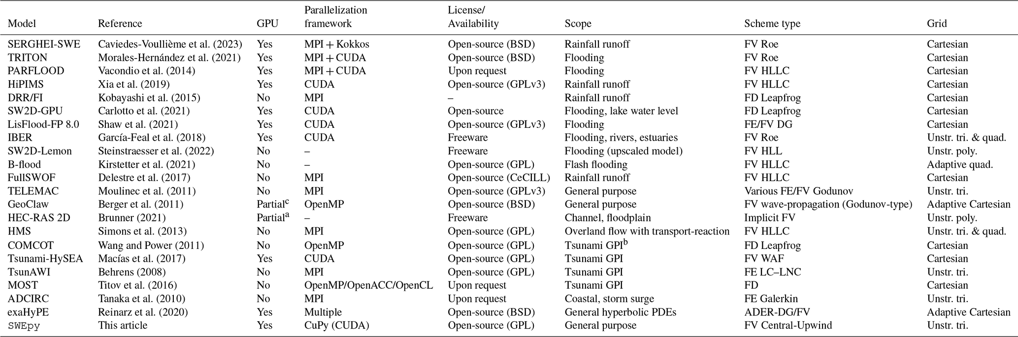
^a GPU support in development (HEC-RAS 2025 Alpha). ^b Generation, Propagation, Inundation. ^c GPU support under active development (not yet merged into the main release).
MPI is available in the dispersive (SGN) version through PETSc.

These programs solve nonlinear SWEs, which have become the cornerstone of two-dimensional free-surface flow modeling across a wide range of applications (Delis and Nikolos, 2021). However, the growing demand for higher spatial resolution and real-time performance has motivated alternative approaches. Some efforts have focused on simplified formulations (Courty et al., 2017) or machine-learning surrogates (Kabir et al., 2020; Zhou et al., 2022; Shaeri Karimi et al., 2019) to reduce computational cost, often at the expense of physical fidelity (Fernández-Pato et al., 2018). In contrast, a more robust strategy relies on parallelization, leveraging high-performance computing on CPUs and GPUs (Caviedes-Voullième et al., 2023; Morales-Hernández et al., 2021; Reinarz et al., 2020) to achieve significant speedups without compromising accuracy.

Indeed, several mature SWE solvers have demonstrated strong performance and robustness in large-scale, real-world applications. Examples include Tsunami-HySEA (Macías et al., 2017), GeoClaw (Berger et al., 2011), MOST (Titov et al., 2016), ADCIRC (Tanaka et al., 2010), exaHYPE (Reinarz et al., 2020), and TsunAWI (Behrens, 2008). These software exploit parallelization through OpenMP, MPI, CUDA, or hybrid approaches, and employ either fixed meshes or adaptive mesh refinement (AMR) to efficiently capture localized dynamics. Their successful deployment in tsunami early-warning systems, coastal hazard analysis, and continental-scale flooding underscores the critical role of scalable high-performance computing in SWE modeling.

Despite their advanced capabilities, many existing solvers are implemented in low-level languages such as FORTRAN, C$++$, or C, and depend on specialized APIs (e.g., CUDA, MPI, or OpenMP). While these choices enable high performance, they can also limit accessibility for users without advanced programming expertise. In contrast, high-level languages like Python provide a more accessible alternative. However, efficient parallelization in Python is not straightforward due to limitations such as the Global Interpreter Lock (Turner and Wouters, 2024). To overcome these challenges, libraries such as Numba (Lam et al., 2015), PyCUDA (Kloeckner et al., 2025), TensorFlow (Abadi et al., 2015), PyTorch (Ansel et al., 2024), and Dask (Rocklin, 2015) enable efficient parallel execution – particularly on GPUs – through compiled kernels and SIMD-based approaches.

In this context, CuPy (Okuta et al., 2017) provides a particularly attractive solution. As a drop-in replacement for NumPy (Harris et al., 2020), CuPy executes array operations using NVIDIA CUDA kernels, enabling seamless GPU acceleration with minimal code modification. By building on the mature CUDA ecosystem, it supports custom kernels, reproducible high-performance execution, and scalable multi-GPU workflows – all while maintaining a user-friendly interface that avoids low-level GPU programming. While today experimental support exists for alternative backends in CuPy, the focus on a well-established CUDA platform provides a robust and reliable foundation for advanced numerical modeling without sacrificing efficiency or accessibility.

Although most SWE solvers incorporate some form of parallelization, they vary significantly in scope, numerical methods, grid geometries, and implementation/parallelization strategies (e.g., CUDA, Kokkos, MPI, or OpenMP). Some are tailored to specific applications, such as rainfall–runoff modeling (e.g., SERGHEI-SWE, HiPIMS) or tsunami generation-propagation-inundation (e.g., COMCOT, Tsunami-HySEA, TsunAWI), while others are designed for more general-purpose simulations. This diversity reflects necessary design trade-offs, but also highlights the lack of a unified framework that combines flexibility across these dimensions.

A key factor influencing both solver performance and applicability is grid discretization. Structured Cartesian grids are widely used due to their simplicity and computational efficiency, particularly when combined with adaptive mesh refinement (AMR). In contrast, unstructured triangular meshes provide greater geometric flexibility, enabling localized refinement in regions with complex bathymetry, irregular coastlines, or urban features without requiring hierarchical grid structures (Schubert et al., 2008). This flexibility makes them especially well-suited for multi-scale problems – such as tsunami propagation coupled with near-shore inundation – where localized resolution is critical, and can eliminate the need for nested grids in complex simulations (Harig et al., 2008; Bomers et al., 2019).

A large class of SWE solvers is based on finite-volume (FV) Godunov-type schemes, which employ approximate Riemann solvers – such as Roe, HLL, or HLLC – to compute numerical fluxes. These methods are well established, robust, and highly optimized for large-scale applications, providing accurate resolution of wave propagation and discontinuities. An alternative class of methods are offered by central-upwind (CU) schemes, which avoid the explicit solution of Riemann problems by estimating local propagation speeds to construct numerical fluxes. Although not intended to replace Riemann-solver-based methods, CU schemes provide a conceptually simpler and more flexible framework, particularly attractive for implementations on unstructured grids and for coupling with high-order reconstruction techniques. Originally introduced for Cartesian grids by Kurganov and Tadmor (2000) and later extended to triangular meshes by Kurganov and Petrova (2005), CU schemes approximate fluxes by integrating over local Riemann fans defined by these estimated speeds.

Despite their advantages, CU formulations for the SWE are often affected by excessive numerical diffusion. Recent efforts to mitigate this issue have largely focused on Cartesian-grid finite-difference formulations (Kurganov and Xin, 2023; Chu et al., 2025; Cui et al., 2025), leaving triangular FV implementations comparatively underexplored. One promising strategy to reduce diffusion while preserving the CU framework is the incorporation of high-order polynomial reconstructions. However, advanced schemes such as ENO/WENO (Zhang and Shu, 2016) introduce significant computational overhead due to large stencils, smoothness indicator evaluations, and potentially complex neighbor-search procedures. In this context, high-performance computing becomes essential. Although high-order WENO schemes can be computationally prohibitive in serial CPU implementations, their high arithmetic intensity makes them particularly well suited for GPU acceleration, where their computational cost can be effectively amortized.

Furthermore, the behavior of the SWE is governed not only by flux terms but also by source terms in the balance equations, as well as domain characteristics such as bathymetry and boundary conditions. This diversity of physical settings requires numerical formulations that can accommodate a broad range of scenarios while maintaining both accuracy and stability. In addition to the choice of numerical flux, the design of spatial discretization plays a critical role and must satisfy key physical and numerical properties, including well-balancing and positivity preservation, as extensively discussed in the literature (e.g., Kurganov and Tadmor, 2000; Kurganov and Petrova, 2005; Toro et al., 1994). Well-balancing ensures the exact preservation of steady states – such as a lake at rest over variable topography or geostrophic equilibrium – thereby preventing spurious oscillations that can degrade accuracy in long-term or large-scale simulations. Positivity preservation, on the other hand, guarantees non-negative water depths, which is essential for stable and physically meaningful solutions near wet-dry interfaces. Achieving these properties requires carefully designed reconstruction operators that are consistently integrated with the underlying numerical scheme.

Motivated by these considerations, we introduce SWEpy, an open-source, Python-based FV solver for the SWE on unstructured triangular grids with GPU acceleration. The proposed framework is designed to overcome limitations of existing approaches by enabling efficient and flexible modeling of both near-field and far-field phenomena within a unified formulation. The main contributions of this work are threefold: (1) the development of a CU scheme extended to higher-order accuracy through quadratic WENO reconstruction and third-order strong-stability-preserving (SSP) Runge–Kutta time integration, reducing numerical diffusion while accurately capturing both shock-dominated and wave-propagation regimes; (2) an open-source release under the GNU General Public License (GPL), promoting transparency, reproducibility, and community-driven development; and (3) a Python/CuPy implementation that enables efficient GPU acceleration on CUDA-compatible hardware, lowering the barrier to high-performance computing while maintaining computational efficiency. SWEpy is designed to be well-balanced and positivity-preserving, and its performance is validated against both canonical benchmarks and real-world applications, including the Malpasset dam-break (near-field inundation) and the 2010 Maule tsunami (basin-scale propagation). Building on these results, the remainder of this paper is organized as follows: Sect. 2 presents the governing equations and FV formulation; Sect. 3 describes the numerical scheme and reconstruction procedures; Sect. 4 details the Python/CuPy implementation; Sect. 5 presents validation and performance results; and Sect. 6 concludes with a discussion of implications and future directions.

2 Problem Setting

This section defines the physical problem, presents the governing equations, and derives the semi-discrete form of the SWEs, which provides the foundation for the CU scheme with WENO reconstruction on unstructured triangular grids implemented in SWEpy.

2.1 Governing Equations

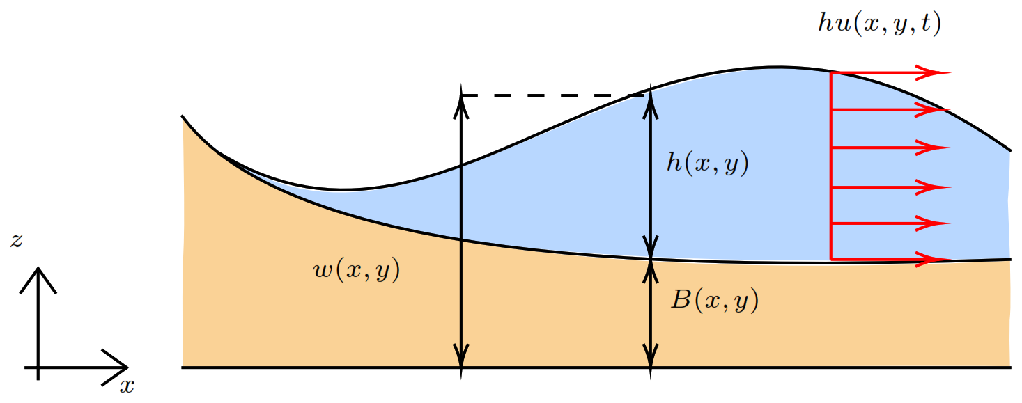
The SWEs, originally introduced in one dimension by Saint-Venant (1871), are obtained in two dimensions through a depth-averaging of the Navier–Stokes equations under the hydrostatic pressure assumption. Assuming incompressibility and an appropriate scaling in which vertical accelerations are negligible, the vertical momentum equation reduces to a hydrostatic pressure distribution. This simplification allows the continuity and horizontal momentum equations to be integrated from the bed to the free surface, yielding a system expressed in terms of depth-averaged variables (Castro-Orgaz and Hager, 2019; Chow et al., 1988; Hervouet, 2007; Vreugdenhil, 1994). The resulting equations constitute the foundation of computational models for free-surface flows in rivers, coastal regions, and urban floodplains, and are capable of describing a wide range of phenomena, including flood waves, tsunamis, and storm surges (Delis and Nikolos, 2021).

To establish a consistent notation, we define the state vector $\mathit{q}=(h,hu,hv{)}^{\top }$, where $h(x,y,t)$ denotes the water depth measured from the bathymetry B(x,y) to the free surface $w(x,y,t)$ relative to the z=0 reference plane. The variables $u(x,y,t)$ and $v(x,y,t)$ represent the depth-averaged velocity components in the x and y directions, while $hu(x,y,t)$ and $hv(x,y,t)$ correspond to the associated discharge fluxes. Scalar quantities (e.g., h) are denoted by regular symbols, whereas vector quantities (e.g., q) are indicated in bold. A schematic representation of these variables is provided in Fig. 1.

Figure 1 Model setting and physical variables used in the SWE.

This definition of variables allows to express the SWEs in conserved vector form as:

$$\begin{array}{}\text{(1)}& {\mathit{q}}_t+\mathit{f}(\mathit{q}{)}_x+\mathit{g}(\mathit{q}{)}_y={\mathit{S}}_{\mathrm{B}}\left(\mathit{q}\right)+\mathit{S}\left(\mathit{q}\right),\end{array}$$

where (⋅)_t, (⋅)_x, and (⋅)_y denote partial derivatives with respect to t, x, and y, respectively. In addition, the associated vector quantities are

$$\begin{array}{}\text{(2)}& {\displaystyle }\mathit{q}=(h,hu,hv{)}^{\top },\text{(3)}& {\displaystyle }\mathit{f}\left(\mathit{q}\right)={\left(hu,h{u}^{\mathrm{2}}+{\displaystyle \frac{g{h}^{\mathrm{2}}}{\mathrm{2}}},huv\right)}^{\top },\text{(4)}& {\displaystyle }\mathit{g}\left(\mathit{q}\right)={\left(hv,huv,h{v}^{\mathrm{2}}+{\displaystyle \frac{g{h}^{\mathrm{2}}}{\mathrm{2}}}\right)}^{\top },\text{and}\text{(5)}& {\displaystyle }{\mathit{S}}_{\mathrm{B}}\left(\mathit{q}\right)={\left(\mathrm{0},-gh{B}_x,-gh{B}_y\right)}^{\top },\end{array}$$

where S(q) denotes additional source terms, including Coriolis forcing, bottom friction, rheological effects, and turbulence.

In this study, we consider bottom friction S_F(q) and Coriolis forcing S_C(q), which are particularly relevant for modeling dam-break flows and large-scale tsunami propagation, respectively. Bottom friction is modeled using the semi-empirical Manning–Strickler formulation (Chow et al., 1988), while the Coriolis term accounts for rotational effects. These source terms are given by

$$\begin{array}{}\text{(6)}& {\displaystyle }{\mathit{S}}_{\mathrm{C}}\left(\mathit{q}\right)={\left(\mathrm{0},fhv,-fhu\right)}^{\top },\text{and}\text{(7)}& {\displaystyle }\begin{array}{rl}{\mathit{S}}_{\mathrm{F}}\left(\mathit{q}\right)& =\left(\mathrm{0},-g{\displaystyle \frac{n^{\mathrm{2}}}{h^{\mathrm{7}/\mathrm{3}}}}hu\sqrt{(hu{)}^{\mathrm{2}}+(hv{)}^{\mathrm{2}}},\right.\\ & {\left.-g{\displaystyle \frac{n^{\mathrm{2}}}{h^{\mathrm{7}/\mathrm{3}}}}hv\sqrt{(hu{)}^{\mathrm{2}}+(hv{)}^{\mathrm{2}}}\right)}^{\top },\end{array}\end{array}$$

where n denotes the Manning friction coefficient and f is the Coriolis parameter, typically approximated as ${\mathrm{10}}^{-\mathrm{4}},{\mathrm{s}}^{-\mathrm{1}}$ (Kundu et al., 2012). For long-range tsunami propagation, both bathymetric and Coriolis source terms (S_B and S_C) are considered, whereas flooding applications incorporate bathymetry and bottom friction (S_B and S_F).

The resulting system of nonlinear hyperbolic equations requires robust numerical methods to accurately capture shocks and maintain stability, particularly in the presence of complex geometries and wet-dry interfaces. These challenges are addressed in SWEpy through a CU scheme on unstructured triangular grids, as detailed in Sect. 3.

2.2 Semi-discrete formulation

FVMs provide a robust framework for solving the SWEs, ensuring conservation of mass and momentum while accurately handling discontinuities such as shocks and wet-dry fronts (LeVeque, 2002; Moukalled et al., 2015; Toro, 2001). In this approach, the governing equations are integrated over discrete control volumes, yielding cell-averaged quantities that are evolved in time through numerical fluxes evaluated at cell interfaces. This formulation naturally captures sharp features, such as hydraulic jumps and bore propagation, without the need for additional artificial viscosity (Stiernström et al., 2021), making it particularly well suited for shallow water flows characterized by abrupt regime transitions.

To improve well-balancing¹, we reformulate the system by expressing the conserved variables in terms of the free-surface elevation $w=h+B$ rather than the water depth h. Specifically, the state vector becomes $\mathit{q}(x,y,t)=(w,hu,hv{)}^{\top }$. This substitution mitigates numerical imbalances associated with topographic gradients and leads to the following system:

$$\begin{array}{}\text{(8)}& {\mathit{q}}_t+\mathit{F}(\mathit{q},B{)}_x+\mathit{G}(\mathit{q},B{)}_y={\mathit{S}}_{\mathrm{B}}(\mathit{q},B)+\mathit{S}(\mathit{q},B),\end{array}$$

where

$$\begin{array}{}\text{(9)}& {\displaystyle }\mathit{F}(\mathit{q},B)={\left(hu,{\displaystyle \frac{(hu{)}^{\mathrm{2}}}{w-B}}+{\displaystyle \frac{\mathrm{1}}{\mathrm{2}}}g(w-B{)}^{\mathrm{2}},{\displaystyle \frac{\left(hu\right)\left(hv\right)}{w-B}}\right)}^{\top },\text{(10)}& {\displaystyle }\mathit{G}(\mathit{q},B)={\left(hv,{\displaystyle \frac{\left(hu\right)\left(hv\right)}{w-B}},{\displaystyle \frac{(hv{)}^{\mathrm{2}}}{w-B}}+{\displaystyle \frac{\mathrm{1}}{\mathrm{2}}}g(w-B{)}^{\mathrm{2}}\right)}^{\top }.\end{array}$$

We then consider a triangular discretization of the polygonal spatial domain $\mathrm{\Omega }={\bigcup }_j{\mathrm{\Omega }}_j$, including additional “ghost” cells for boundary conditions, as displayed in Fig. 2 (bottom border). Integrating Eq. (8) over each cell Ω_j and applying the Gauss divergence theorem yields:

$$\begin{array}{}\text{(11)}& {\displaystyle \frac{d}{\mathrm{d}t}}\underset{{\mathrm{\Omega }}_j}{\int }\mathit{q}\mathrm{d}\mathrm{\Omega }+\underset{\partial {\mathrm{\Omega }}_j}{\oint }(\mathit{F},\mathit{G}){\widehat{\mathit{n}}}_j\mathrm{d}{l}_j=\underset{\mathrm{\Omega }}{\int }({\mathit{S}}_B+\mathit{S})\mathrm{d}\mathrm{\Omega }.\end{array}$$

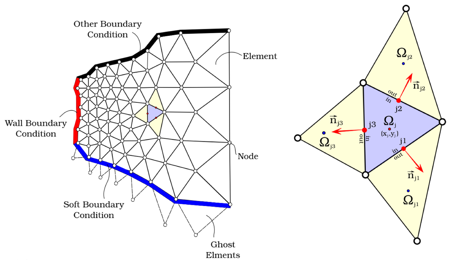
Figure 2 Illustration of a triangular unstructured grid. The figure shows on the left an example of a finite volume grid, while on the right a typical triangular cell with some attributes used in the semi-discrete formulation.

Let Ω_jk ($k=\mathrm{1},\mathrm{2},\mathrm{3}$) denote the cells neighboring Ω_j. Now, let (x_j,y_j) be the barycenter of Ω_j, and Γ_jk the edge shared with Ω_jk, with length l_jk. The outward unit normal vector to Γ_jk is given by ${\widehat{\mathit{n}}}_{jk}=\left(\cos \left({\mathit{\theta }}_{jk}\right),\sin \left({\mathit{\theta }}_{jk}\right)\right)$, where θ_jk denotes its orientation. Then, the semi-discrete formulation is written as

$$\begin{array}{}\text{(12)}& {\displaystyle \frac{d}{\mathrm{d}t}}{\stackrel{\mathrm{‾}}{\mathit{q}}}_j\left(t\right)+{\displaystyle \frac{\mathrm{1}}{\mathrm{|}{\mathrm{\Omega }}_j\mathrm{|}}}\sum _{k\in {\mathcal{N}}_j}{\mathcal{F}}_{jk}{l}_{jk}={\stackrel{\mathrm{‾}}{\mathit{S}}}_{{\mathrm{B}}_j}+{\stackrel{\mathrm{‾}}{\mathit{S}}}_j,\end{array}$$

where ${\stackrel{\mathrm{‾}}{\mathit{q}}}_j=\frac{\mathrm{1}}{\left|\mathrm{\Omega }j\right|}{\int }_{{\mathrm{\Omega }}_j}\mathit{q}(x,y,t)\mathrm{d}\mathrm{\Omega }$ denotes the cell-averaged state, and ℱ_jk is the numerical flux across the interface Γ_jk, accounting for interactions between neighboring cells. This flux is constructed from the physical flux functions F and G in Eq. (9) and depends on reconstructed states at the interface, denoted ${\mathit{q}}_{jk}^{\text{in}}$ and ${\mathit{q}}_{jk}^{\text{out}}$, obtained via suitable reconstruction operators.

The boundary integrals are evaluated using Gaussian quadrature, with the number of quadrature points determined by the order of the reconstruction. Since the reconstructed states are time-dependent, Eq. (12) defines a system of ordinary differential equations that needs to be integrated numerically. In this equation, the terms ${\stackrel{\mathrm{‾}}{\mathit{S}}}_{{\mathrm{B}}_j}$ and ${\stackrel{\mathrm{‾}}{\mathit{S}}}_j$ represent consistent discretizations of the bathymetric and additional source terms, respectively, and will be detailed in the following sections. This formulation provides the basis for the CU discretization described in Sect. 3.

3 SWEpy Numerical Model

Building on the semi-discrete formulation, SWEpy employs a CU FVM for solving hyperbolic conservation laws on unstructured triangular grids. This approach was originally introduced by Kurganov and Petrova (2005), with parallel developments addressing well-balancing and related formulations by Bryson and Levy (2005) and Xie et al. (2005), and further refined in subsequent studies. This section presents a concise description of the numerical formulation adopted in this work.

3.1 Central-Upwind Numerical Fluxes on Triangular Grids

The CU scheme avoids the explicit solution of Riemann problems by estimating local wave propagation speeds to construct numerical fluxes. This results in a method that balances computational simplicity with robustness, making it particularly well suited for shallow water flows over complex geometries, including variable bathymetry and wet-dry interfaces.

The numerical flux ℱ_jk in Eq. (12) is formulated as the projection onto the edge-normal direction Γ_jk:

$$\begin{array}{}\text{(13)}& \begin{array}{rl}{\mathcal{F}}_{jk}& =\left(F_{jk}\cos \right({\mathit{\theta }}_{jk})+G_{jk}\sin ({\mathit{\theta }}_{jk}\left)\right)-{\displaystyle \frac{a_{jk}^{\text{in}}{a}_{jk}^{\mathrm{out}}}{a_{jk}^{\text{in}}+a_{jk}^{\text{out}}}}\\ & \sum _{s=\mathrm{1}}^{N_s}{c}_s\left[{\mathit{q}}_{jk}^{\text{in}}\right(M_{jk}^s)-{\mathit{q}}_{jk}^{\text{out}}(M_{jk}^s\left)\right],\end{array}\end{array}$$

where $M_{jk}^s$ are the Gaussian quadrature points along the edge, and c_s are the associated weights. The number of integration points N_s depends on the reconstruction order to ensure accurate integration. The terms $a_{jk}^{\text{in}}$ and $a_{jk}^{\text{out}}$ represent the inward and outward local propagation speeds, given in Eq. (19). In addition, the flux projection components in Eq. (13) are:

$$\begin{array}{}\text{(14)}& {\displaystyle }\begin{array}{rl}{F}_{jk}& ={\displaystyle \frac{\mathrm{1}}{a_{jk}^{\text{in}}+a_{jk}^{\text{out}}}}\sum _{s=\mathrm{1}}^{N_s}{c}_s\left[a_{jk}^{\text{in}}\mathit{F}\left({\mathit{q}}_{jk}^{\text{in}}\left(M_{jk}^s\right),B\left(M_{jk}^s\right)\right)\right.\\ & \left.+a_{jk}^{\text{out}}\mathit{F}\left({\mathit{q}}_{jk}^{\text{out}}\left(M_{jk}^s\right),B\left(M_{jk}^s\right)\right)\right],\text{and}\end{array}\text{(15)}& {\displaystyle }\begin{array}{rl}{G}_{jk}& ={\displaystyle \frac{\mathrm{1}}{a_{jk}^{\text{in}}+a_{jk}^{\text{out}}}}\sum _{s=\mathrm{1}}^{N_s}{c}_s\left[a_{jk}^{\text{in}}\mathit{G}\left({\mathit{q}}_{jk}^{\text{in}}\left(M_{jk}^s\right),B\left(M_{jk}^s\right)\right)\right.\\ & \left.+a_{jk}^{\text{out}}\mathit{G}\left({\mathit{q}}_{jk}^{\text{out}}\left(M_{jk}^s\right),B\left(M_{jk}^s\right)\right)\right].\end{array}\end{array}$$

In Eqs. (14) and (15), the vectors ${\mathit{q}}_{jk}^{\text{out}}$ and ${\mathit{q}}_{jk}^{\text{in}}$ denote the limiting values of q(x,y) at the interface point $M_{jk}^s$ approached from within Ω_j and Ω_jk, respectively. Moreover, due to the form of the fluxes F_jk and G_jk, divisions by zero may arise near wet–dry interfaces. To prevent such singularities, a consistent flux treatment is required, as addressed through the positivity-preserving reconstruction described in Sect. 3.4.

Substituting Eqs. (13), (14) and (15) into Eq. (12) yields

$$\begin{array}{}\text{(16)}& \begin{array}{rl}& {\displaystyle \frac{\mathrm{d}{\stackrel{\mathrm{‾}}{\mathit{q}}}_j}{\mathrm{d}t}}=-{\displaystyle \frac{\mathrm{1}}{\left|{\mathrm{\Omega }}_j\right|}}\sum _{k=\mathrm{1}}^{\mathrm{3}}{\displaystyle \frac{l_{jk}\cos {\mathit{\theta }}_{jk}}{a_{jk}^{\text{in}}+a_{jk}^{\text{out}}}}\sum _{s=\mathrm{1}}^{N_s}{c}_s\\ & \left[a_{jk}^{\text{in}}\mathit{F}\left({\mathit{q}}_{jk}\left(M_{jk}^s\right),B\left(M_{jk}^s\right)\right)+a_{jk}^{\text{out}}\mathit{F}\left({\mathit{q}}_j\left(M_{jk}^s\right),B\left(M_{jk}^s\right)\right)\right]\\ & -{\displaystyle \frac{\mathrm{1}}{\left|{\mathrm{\Omega }}_j\right|}}\sum _{k=\mathrm{1}}^{\mathrm{3}}{\displaystyle \frac{l_{jk}\sin {\mathit{\theta }}_{jk}}{a_{jk}^{\text{in}}+a_{jk}^{\text{out}}}}\sum _{s=\mathrm{1}}^{N_s}{c}_s\left[a_{jk}^{\text{in}}\mathit{G}\left({\mathit{q}}_{jk}\left(M_{jk}^s\right),B\left(M_{jk}^s\right)\right)\right.\\ & \left.+a_{jk}^{\text{out}}\mathit{G}\left({\mathit{q}}_j\left(M_{jk}^s\right),B\left(M_{jk}^s\right)\right)\right]\\ & +{\displaystyle \frac{\mathrm{1}}{\left|{\mathrm{\Omega }}_j\right|}}\sum _{k=\mathrm{1}}^{\mathrm{3}}{l}_{jk}{\displaystyle \frac{a_{jk}^{\text{in}}{a}_{jk}^{\text{out}}}{a_{jk}^{\text{in}}+a_{jk}^{\text{out}}}}\sum _{s=\mathrm{1}}^{N_s}{c}_s\left[{\mathit{q}}_{jk}\left(M_{jk}^s\right)-{\mathit{q}}_j\left(M_{jk}^s\right)\right]\\ & +{\stackrel{\mathrm{‾}}{\mathit{S}}}_{{\mathrm{B}}_j}+{\stackrel{\mathrm{‾}}{\mathit{S}}}_j,\end{array}\end{array}$$

where ${\stackrel{\mathrm{‾}}{\mathit{q}}}_j$ is the cell-averaged state, the bathymetry $B\left(M_{jk}^s\right)$ follows the same reconstruction criterion as the flux variables, and ${\stackrel{\mathrm{‾}}{\mathit{S}}}_j$ is the discretized source term, discussed in the following subsection.

The one-sided local speeds² $a_{jk}^{\text{in}}$ and $a_{jk}^{\text{out}}$ are evaluated at Gaussian quadrature points using desingularized velocities to ensure stable behavior near dry states. The velocity components are regularized as

$$\begin{array}{}\text{(17)}& u={\displaystyle \frac{\sqrt{\mathrm{2}},h\left(hu\right)}{\sqrt{h^{\mathrm{4}}+max(h^{\mathrm{4}},\mathit{\epsilon })}}},\text{and}v={\displaystyle \frac{\sqrt{\mathrm{2}},h\left(hv\right)}{\sqrt{h^{\mathrm{4}}+max(h^{\mathrm{4}},\mathit{\epsilon })}}},\end{array}$$

where $h=w-B$ denotes the water depth and ε is a small tolerance parameter that prevents singularities as h→0. These velocities are then projected onto the outward normal direction of the interface Γ_jk, yielding

$$\begin{array}{}\text{(18)}& \begin{array}{rl}{u}_j^{\mathit{\theta }}\left(M_{jk}^s\right)& =\cos \left({\mathit{\theta }}_{jk}\right),u_j\left(M_{jk}^s\right)+\sin \left({\mathit{\theta }}_{jk}\right),v_j\left(M_{jk}^s\right)\\ & \text{and}{u}_{jk}^{\mathit{\theta }}\left(M_{jk}^s\right)=\cos \left({\mathit{\theta }}_{jk}\right),u_{jk}\left(M_{jk}^s\right)\\ & +\sin \left({\mathit{\theta }}_{jk}\right),v_{jk}\left(M_{jk}^s\right)\end{array}\end{array}$$

where the subscripts j and jk denote reconstructed values from cell Ω_j and its neighbor Ω_jk, respectively.

The one-sided local wave speeds are then obtained by taking extrema over all Gaussian points:

$$\begin{array}{}\text{(19)}& \begin{array}{rl}{a}_{jk}^{\text{out}}& =\underset{s}{max}\left\{max\left\{u_j^{\mathit{\theta }}\left(M_{jk}^s\right)+\sqrt{g{h}_j\left(M_{jk}^s\right)},u_{jk}^{\mathit{\theta }}\left(M_{jk}^s\right)\right.\right.\\ & \left.\left.+\sqrt{g{h}_{jk}\left(M_{jk}^s\right)},\mathrm{0}\right\}\right\},\\ & a_{jk}^{\text{in}}=-\underset{s}{min}\left\{min\left\{u_j^{\mathit{\theta }}\left(M_{jk}^s\right)-\sqrt{g{h}_j\left(M_{jk}^s\right)},u_{jk}^{\mathit{\theta }}\left(M_{jk}^s\right)\right.\right.\\ & \left.\left.-\sqrt{g{h}_{jk}\left(M_{jk}^s\right)},\mathrm{0}\right\}\right\}.\end{array}\end{array}$$

3.2 Well-balancing of the source terms

A fundamental requirement for robust SWE solvers – particularly in applications involving complex topography such as dam-break flows and tsunamis – is well-balancing. This property is defined as the exact preservation of steady-state solutions without introducing spurious oscillations. Well-balance is essential for maintaining physical accuracy in scenarios such as the lake-at-rest condition or geostrophic equilibrium, where source terms must precisely counterbalance flux gradients (Kurganov and Petrova, 2007; Bryson et al., 2011; Liu et al., 2018; Chertock et al., 2015, 2018; Desveaux and Masset, 2022; Greenberg and Leroux, 1996; Liu, 2021b; Cao et al., 2024). Therefore, in SWEpy, well-balancing is achieved through a consistent discretization of the source terms, ensuring that numerical fluxes remain in equilibrium with the underlying physical forces across both fully wet domains and regions with variable bathymetry.

3.2.1 Bathymetry gradient contribution

For the bathymetry source term, a well-balanced discretization is constructed by enforcing the lake-at-rest condition, ensuring consistency with the corresponding momentum flux contributions (Bryson et al., 2011). Thus, variables are first reconstructed using polynomial approximations, after which the resulting expressions are integrated over both the cell and its interfaces using Gaussian quadrature. This procedure yields a general formulation that is applicable to arbitrary reconstruction orders:

$$\begin{array}{}\text{(20)}& \begin{array}{rl}& {\stackrel{\mathrm{‾}}{\mathit{S}}}_{{\mathrm{B}}_j}^{\left(l\right)}=-g\sum _{s=\mathrm{1}}^{N_s^{\mathrm{int}}}{c}_s{\displaystyle \frac{\partial w\left(M_j^s\right)}{\partial x}}\left(w_j\right(M_j^s)-B(M_j^s\left)\right)\\ & +{\displaystyle \frac{g}{\mathrm{2}\left|{\mathrm{\Omega }}_j\right|}}\sum _{k=\mathrm{1}}^{\mathrm{3}}\sum _{s=\mathrm{1}}^{N_s}{c}_s{l}_{jk}\left(w_j\right(M_{jk}^s)-B(M_{jk}^s){)}^{\mathrm{2}}\cos {\mathit{\theta }}_{jk},\\ & {\stackrel{\mathrm{‾}}{\mathit{S}}}_{{\mathrm{B}}_j}^{\left(\mathrm{3}\right)}=-g\sum _{s=\mathrm{1}}^{N_s^{\mathrm{int}}}{c}_s{\displaystyle \frac{\partial w\left(M_j^s\right)}{\partial y}}\left(w_j\right(M_j^s)-B(M_j^s\left)\right)\\ & +{\displaystyle \frac{g}{\mathrm{2}\left|{\mathrm{\Omega }}_j\right|}}\sum _{k=\mathrm{1}}^{\mathrm{3}}\sum _{s=\mathrm{1}}^{N_s}{c}_s{l}_{jk}\left(w_j\right(M_{jk}^s)-B(M_{jk}^s){)}^{\mathrm{2}}\sin {\mathit{\theta }}_{jk},\end{array}\end{array}$$

In Eq. (20), $N_s^{\text{int}}$ denotes the number of Gaussian quadrature points $M_j^s$ used over the cell interior Ω_j, and c_s are the corresponding weights. The bathymetry B is reconstructed using the same-order operator employed for the flow variables, ensuring consistency in the discretization.

This formulation enforces a consistent balance between source terms and flux contributions, eliminating spurious flows over irregular topography and ensuring the preservation of equilibrium states, as verified in the steady-state benchmarks in Sect. 5.

3.2.2 Manning friction

The structure of the Manning friction source term allows for a straightforward well-balanced discretization, as it is directly proportional to the discharge components $\stackrel{\mathrm{‾}}{hu}$ and $\stackrel{\mathrm{‾}}{hv}$. Consequently, the term vanishes at equilibrium without requiring additional modifications. However, near wet–dry interfaces or in regions where h→0, desingularization is necessary to avoid division by zero and ensure numerical stability.

Following Chertock et al. (2015), we define the discrete friction coefficient as

$$\begin{array}{}\text{(21)}& \begin{array}{rl}\mathcal{G}\left({\stackrel{\mathrm{‾}}{\mathit{q}}}_j\right):& =-g{n}^{\mathrm{2}}{\left({\displaystyle \frac{\mathrm{2}{\stackrel{\mathrm{‾}}{h}}_j}{{\stackrel{\mathrm{‾}}{h}}_j^{\mathrm{2}}+max\left({\stackrel{\mathrm{‾}}{h}}_j^{\mathrm{2}},{\mathit{\epsilon }}^{\mathrm{2}}\right)}}\right)}^{\mathrm{7}/\mathrm{3}}\\ & \sqrt{(\stackrel{\mathrm{‾}}{hu}{)}_j^{\mathrm{2}}+(\stackrel{\mathrm{‾}}{hv}{)}_j^{\mathrm{2}}},\end{array}\end{array}$$

where ${\stackrel{\mathrm{‾}}{h}}_j={\stackrel{\mathrm{‾}}{w}}_j-{\stackrel{\mathrm{‾}}{B}}_j$ denotes the cell-averaged water depth and ε is a small regularization parameter introduced to avoid singularities.

The corresponding discretized friction source term is then given by

$$\begin{array}{}\text{(22)}& {\stackrel{\mathrm{‾}}{\mathit{S}}}_{{\mathrm{F}}_j}=\mathcal{G}\left({\stackrel{\mathrm{‾}}{\mathit{q}}}_j\right){\left[\begin{array}{ccc}\mathrm{0}& (\stackrel{\mathrm{‾}}{hu}{)}_j& (\stackrel{\mathrm{‾}}{hv}{)}_j\end{array}\right]}^T.\end{array}$$

This formulation is treated semi-implicitly during time integration, as described in Sect. 3.5, to account for the stiffness of the friction source term (Chertock et al., 2015). In SWEpy, the coefficient 𝒢 is evaluated in a vectorized manner across all cells on the GPU, enabling efficient parallel computation even for large-scale grids. Although the Manning coefficient n may vary spatially, it is taken as constant throughout the domain in the presented numerical experiments.

3.2.3 Coriolis

The Coriolis source term vanishes under zero-discharge equilibria (i.e., $hu=hv=\mathrm{0}$), ensuring inherent well-balancing in such states without requiring specialized discretization beyond direct averaging. Accordingly, the cell-averaged Coriolis source term is:

$$\begin{array}{}\text{(23)}& ({\stackrel{\mathrm{‾}}{\mathit{S}}}_{\mathrm{C}}{)}_j=f{\left[\begin{array}{ccc}\mathrm{0}& (\stackrel{\mathrm{‾}}{hv}{)}_j& -(\stackrel{\mathrm{‾}}{hu}{)}_j\end{array}\right]}^{\top },\end{array}$$

where f is the Coriolis parameter, typically approximated as ${\mathrm{10}}^{-\mathrm{4}}{\mathrm{s}}^{-\mathrm{1}}$ in mid-latitude regions (Kundu et al., 2012), as adopted in the Maule 2010 tsunami validation in Sect. 5.2.2.

For large-scale geophysical flows, however, a more rigurous condition – geostrophic balance – may be required. In this regime, horizontal pressure gradients are balanced by Coriolis forces, leading to nontrivial steady states. Several numerical approaches have been proposed to preserve this balance in rotating SWEs (Desveaux and Masset, 2022; Chertock et al., 2018). In the present work, SWEpy employs standard well-balancing, with extensions toward geostrophic preservation left for future development.

3.3 Spatial Reconstruction Operators and Scheme Formulation

The design of these reconstruction operators is guided by both physical and numerical requirements inherent to shallow water flows, including variable bathymetry, surface roughness, and domain scale. These features demand accurate representation of gradients and discontinuities, particularly in near-field regimes (e.g., shocks and wet–dry fronts) and far-field wave propagation, as demonstrated in Sect. 5.

To ensure physically meaningful and numerically stable solutions, the reconstruction must satisfy key properties. These include well-balancing, which guarantees the exact preservation of steady states – such as lake-at-rest or geostrophic equilibrium – thereby preventing spurious oscillations (Bryson et al., 2011), and positivity preservation, which enforces non-negative water depths and is essential for realistic inundation modeling.

Numerical experiments involving long-range tsunami propagation (in Sect. 5) indicate that low-order reconstructions (constant or linear) introduce excessive numerical diffusion, leading to significant attenuation of wave amplitudes. This motivates the use of higher-order reconstruction operators. Accordingly, the reconstructed variables are represented as piecewise polynomials over each cell Ω_j, given by:

$$\begin{array}{}\text{(24)}& {\stackrel{\mathrm{̃}}{q}}_j(x,y)={\stackrel{\mathrm{‾}}{q}}_j+p_j^q(x,y),\end{array}$$

where ${\stackrel{\mathrm{‾}}{q}}_j$ is the cell-averaged variable to be reconstructed, $p_j^q$ the interpolating polynomial with coefficients derived from local geometry and neighboring variable cell-averaged values. This cell-wise approach allows tailored approximations, with stencil selection critical for accuracy and stability.

Figure 3 illustrates the stencil structure, where Ω_j0 (red) is the reference cell, surrounded by first-order neighbors (blue) and second-order neighbors (green). For each Ω_j0, the stencils are defined as

$$\begin{array}{rl}& \mathit{\{}{\mathrm{\Omega }}_{j_{\mathrm{0}}},{\mathrm{\Omega }}_{j_{\mathrm{1}}},{\mathrm{\Omega }}_{j_{\mathrm{2}}},{\mathrm{\Omega }}_{j_{\mathrm{3}}}\mathit{\}};\mathit{\{}{\mathrm{\Omega }}_{j_{\mathrm{0}}},{\mathrm{\Omega }}_{j_{\mathrm{1}}},{\mathrm{\Omega }}_{j_{\mathrm{11}}},{\mathrm{\Omega }}_{j_{\mathrm{12}}}\mathit{\}};\\ & \mathit{\{}{\mathrm{\Omega }}_{j_{\mathrm{0}}},{\mathrm{\Omega }}_{j_{\mathrm{2}}},{\mathrm{\Omega }}_{j_{\mathrm{21}}},{\mathrm{\Omega }}_{j_{\mathrm{22}}}\mathit{\}};\mathit{\{}{\mathrm{\Omega }}_{j_{\mathrm{0}}},{\mathrm{\Omega }}_{j_{\mathrm{3}}},{\mathrm{\Omega }}_{j_{\mathrm{31}}},{\mathrm{\Omega }}_{j_{\mathrm{32}}}\mathit{\}}.\end{array}$$

Linear reconstructions use only the first stencil, Ω_ji, whereas quadratic reconstructions – requiring two Gaussian points per edge – utilize the full stencil, Ω_jkl. The right panel of Fig. 3 illustrates the selection of these sub-stencils, where the barycenters of the selected cells are constrained to lie within cones defined by lines connecting the reference cell’s barycenter to its vertices.

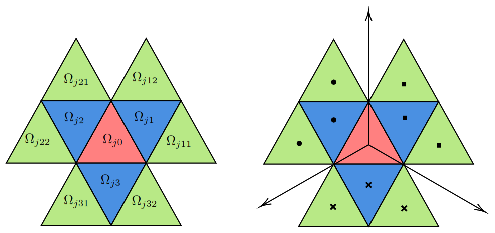
Figure 3 Stencil illustration for the jth cell (left) and its sectorial division (right). The blue triangles represent first-order neighbors Ω_jk, while the green triangles denote second-order neighbors Ω_jkl.

3.3.1 Linear Piecewise Reconstruction with Minmod Gradient Limiter

The linear reconstruction in Eq. (24) is expressed as

$$\begin{array}{}\text{(25)}& {\stackrel{\mathrm{̃}}{q}}_j(x,y)={\stackrel{\mathrm{‾}}{q}}_j+\left(q_x{)}_j\right(x-x_j)+(q_y{)}_j(y-y_j),\end{array}$$

where $D{q}_j=\left(\right(q_x{)}_j,\left(q_y{)}_j\right)$ denotes the numerical gradient.

The selection of this gradient defines the linear reconstruction. A variety of gradient estimation techniques exists in the literature, including classical limiter-based methods (Nessyahu and Tadmor, 1990; Sweby, 1984; Van Leer, 1997), FV formulations (Arminjon and St-Cyr, 2003; Christov and Popov, 2008; Jawahar and Kamath, 2000; LeVeque, 2002), and CU schemes for the Saint-Venant system (Bryson et al., 2011; Kurganov and Petrova, 2005).

In SWEpy, we follow Bryson et al. (2011) and construct three conservative linear polynomials $L_{k,l}^j(x,y)$ over the cell Ω_j and its neighboring pairs Ω_j,k and Ω_j,l (see Fig. 3). The candidate gradient is defined as

$$\begin{array}{}\text{(26)}& q_j^{\prime }=\mathit{\vartheta }\text{minmod}\mathit{\left\{}\mathrm{\nabla }{L}_{k,l}^j\mathit{\right\}},\text{with}\mathit{\theta }\in [\mathrm{1},\mathrm{2}].\end{array}$$

If substituting $q_j^{\prime }$ into Eq. (25) yields values at edge midpoints that exceed local extrema, the reconstruction is reduced to a constant state equal to the cell average; otherwise, the gradient is accepted, i.e., $D{q}_j=q_j^{\prime }$.

The minmod operator presented by Bryson et al. (2011), selects the admissible gradient with the smallest magnitude, thereby limiting spurious oscillations while preserving monotonicity. This ensures consistency with the source term discretization and supports well-balancing. However, it may introduce numerical diffusion in smooth regions, as observed in Sect. 5. A summary of the procedure is provided in Algorithm A1 in the Appendix.

3.3.2 Quadratic (WENO)

To reduce the numerical diffusion observed in low-order reconstructions – particularly in long-range wave propagation (e.g., tsunami simulations in Sect. 5) – we implement a quadratic weighted essentially non-oscillatory (WENO) reconstruction. The approach follows Zhu and Qiu (2018) and is adapted to unstructured triangular grids as in Sunder et al. (2021), while preserving the spatial constraints required for stability.

The reconstruction combines a quadratic polynomial p₀, obtained over the full stencil, with four linear polynomials p_k,j ($k=\mathrm{1},\mathrm{\dots },\mathrm{4}$) defined on sub-stencils:

$$\begin{array}{}\text{(27)}& \begin{array}{rl}{\stackrel{\mathrm{̃}}{q}}_j(x,y)& ={\displaystyle \frac{w_{\mathrm{0}}}{{\mathit{\gamma }}_{\mathrm{0}}}}\left(p_{\mathrm{0}}(x,y)-\sum _{k=\mathrm{1}}^{\mathrm{4}}{\mathit{\gamma }}_k{p}_{k,j}(x,y)\right)\\ & +\sum _{k=\mathrm{1}}^{\mathrm{4}}{w}_k{p}_{k,j}(x,y),\end{array}\end{array}$$

where the nonlinear weights w₀,w_k are computed from smoothness indicators β₀ (quadratic) and β_k (linear) according to $w_l={\stackrel{\mathrm{‾}}{w}}_l/(w_{\mathrm{0}}+{\sum }_{k=\mathrm{1}}^{\mathrm{4}}{\stackrel{\mathrm{‾}}{w}}_k)$, with ${\stackrel{\mathrm{‾}}{w}}_l={\mathit{\gamma }}_l\left(\mathrm{1}+\mathit{\tau }/(\mathit{ϵ}+{\mathit{\beta }}_l)\right)$ and τ a correction term derived from the β_l values (Zhu and Qiu, 2018). The quadratic interpolant p_q,j is constructed via a least-squares fit to the cell-averaged states over Ω_j and its first- and second-order neighbors, while preserving the mean value in Ω_j. Its implementation relies solely on geometric quantities (e.g., barycenters and area moments), avoiding numerical quadrature and improving efficiency, as detailed in (Fuenzalida Alarcón et al., 2025).

The stencil selection is performed efficiently using index-based searches on structured grids; more general geometric search strategies can be incorporated to relax grid constraints. The overall procedure is summarized in Algorithm A2, and is designed for efficient GPU parallelization within SWEpy.

This WENO reconstruction achieves high-order accuracy in smooth regions while limiting oscillations near sharp gradients, making it particularly suitable for far-field simulations where controlling numerical diffusion is critical without relying on Riemann solvers (Kurganov and Petrova, 2005).

3.4 Wet/dry fronts reconstruction

High-order reconstructions, while effective in reducing numerical diffusion in smooth regions, may produce nonphysical negative water depths near wet–dry interfaces, where the free surface intersects the bathymetry. To enforce positivity – i.e., h≥0 – we adopt the conservative correction of Bryson et al. (2011). When negative depths are detected, the reconstruction is replaced by a linear polynomial that preserves the cell average, thereby maintaining mass conservation.

The correction depends on the number of dry vertices. If two vertices are dry, the reconstructed surface is defined by a plane passing through those vertices at bathymetric elevation and the cell barycenter at the mean surface level. If only one vertex is dry, the plane passes through the dry vertex at bathymetry, a neighboring wet vertex at an adjusted elevation, and the barycenter. In both cases, the plane is constructed to ensure $h=w-B\ge \mathrm{0}$ throughout the cell while preserving the mean value.

In practice, reverting locally to a first-order, positivity-preserving reconstruction at wet–dry fronts provides improved robustness with minimal impact on overall accuracy, since high-order reconstruction remains active away from these regions and governs wave propagation. A schematic illustration of this procedure is shown in Fig. 4.

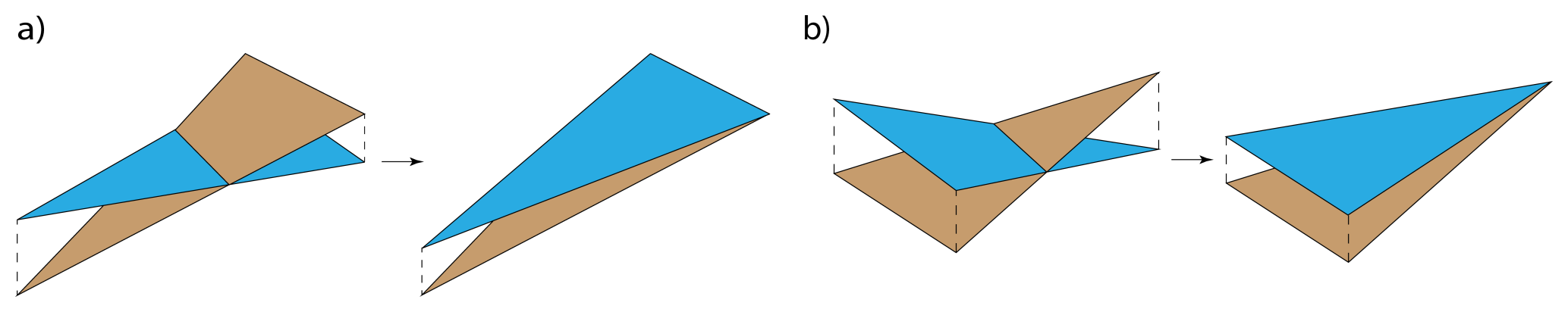
Figure 4 Schematic representation of the wet/dry treatment: (a) two dry points and (b) one dry point.

This approach guarantees non-negative water depths across the domain, which is essential for stability in inundation problems such as the Conical Island test and the Malpasset dam-break case (Sect. 5). The correction procedure is summarized in Algorithm A3 and implemented efficiently using GPU-based parallelization.

While this method ensures positivity, it does not strictly preserve well-balancing near wet–dry fronts, where small imbalances may arise (Liu et al., 2018). This behavior was examined using the analytical solution of Synolakis for wave run-up³, where the method demonstrates good accuracy in the wet–dry region. The results also reveal sensitivity to temporal discretization and the Courant number. A detailed analysis of these aspects is the subject of ongoing work, focusing on the numerical and theoretical properties of wet–dry reconstruction techniques and their suitability for different flow regimes.

3.5 Temporal discretization

Following the spatial discretization, the resulting semi-discrete system of Eq. (12) is integrated in time to ensure stability and accuracy across different flow regimes. In SWEpy, we employ both the explicit Euler (EE) method and a four-stage, third-order strong stability-preserving Runge–Kutta scheme (SSP RK4,3, hereafter RK4,3) described by Gottlieb et al. (2001).

For flows involving Manning friction, a semi-implicit treatment is adopted to improve stability while maintaining computational efficiency (Chertock et al., 2015). We define the discrete flux operator as

$$\begin{array}{}\text{(28)}& {\mathcal{H}}_j({\stackrel{\mathrm{‾}}{\mathit{q}}}_j,{\stackrel{\mathrm{̃}}{\mathit{q}}}_j)=-{\displaystyle \frac{\mathrm{1}}{\mathrm{|}{\mathrm{\Omega }}_j\mathrm{|}}}\sum _{k\in {\mathcal{N}}_j}\left({\mathcal{F}}_{jk}\right)l_{jk}+{\stackrel{\mathrm{‾}}{\mathit{S}}}_{{\mathrm{B}}_j},\end{array}$$

where ${\stackrel{\mathrm{‾}}{\mathit{q}}}_j$ denotes the cell-averaged conserved variables and ${\stackrel{\mathrm{̃}}{\mathit{q}}}_j$ their reconstructions.

The semi-implicit Runge–Kutta update, written in Shu–Osher form, reads

$$\begin{array}{}\text{(29)}& \begin{array}{rl}({\stackrel{\mathrm{‾}}{\mathit{q}}}_j{)}^i& =\sum _{l=\mathrm{0}}^{i-\mathrm{1}}{\mathit{\alpha }}_{i,l}({\stackrel{\mathrm{‾}}{\mathit{q}}}_j{)}^l+{\displaystyle \frac{\mathrm{\Delta }t}{\mathrm{2}}}\sum _{l=\mathrm{0}}^{i-\mathrm{1}}{\mathit{\beta }}_{i,l}{\mathcal{H}}_j^l\\ & +\mathrm{\Delta }t\left(\mathcal{G}\right({\stackrel{\mathrm{‾}}{\mathit{q}}}_j){)}^{i-\mathrm{1}}{\left[\begin{array}{ccc}\mathrm{0}& \left({\stackrel{\mathrm{‾}}{hu}}_j^i\right)& \left({\stackrel{\mathrm{‾}}{hv}}_j^i\right)\end{array}\right]}^T,\\ & i=\mathrm{1},\mathrm{2},\mathrm{3},\mathrm{4}\end{array}\end{array}$$

where ${\stackrel{\mathrm{‾}}{\mathit{q}}}_j^l$ are intermediate stage values, with ${\stackrel{\mathrm{‾}}{\mathit{q}}}_j^{\mathrm{0}}={\stackrel{\mathrm{‾}}{\mathit{q}}}_j^{\left(n\right)}$ and ${\stackrel{\mathrm{‾}}{\mathit{q}}}_j^{(n+\mathrm{1})}={\stackrel{\mathrm{‾}}{\mathit{q}}}_j^{\mathrm{4}}$. The nonzero RK4,3 coefficients are

$$\begin{array}{}\text{(30)}& \begin{array}{rcl}\left(\begin{array}{ccccc}{\mathit{\alpha }}_{\mathrm{1},\mathrm{0}}& {\mathit{\alpha }}_{\mathrm{2},\mathrm{1}}& {\mathit{\alpha }}_{\mathrm{3},\mathrm{0}}& {\mathit{\alpha }}_{\mathrm{3},\mathrm{2}}& {\mathit{\alpha }}_{\mathrm{4},\mathrm{3}}\end{array}\right)& =& \left(\begin{array}{ccccc}\mathrm{1}& \mathrm{1}& \mathrm{2}/\mathrm{3}& \mathrm{1}/\mathrm{3}& \mathrm{1}\end{array}\right),\\ \left(\begin{array}{cccc}{\mathit{\beta }}_{\mathrm{1},\mathrm{0}}& {\mathit{\beta }}_{\mathrm{2},\mathrm{1}}& {\mathit{\beta }}_{\mathrm{3},\mathrm{2}}& {\mathit{\beta }}_{\mathrm{4},\mathrm{3}}\end{array}\right)& =& \left(\begin{array}{cccc}\mathrm{1}& \mathrm{1}& \mathrm{1}/\mathrm{3}& \mathrm{1}\end{array}\right).\end{array}\end{array}$$

The EE scheme follows directly with ${\mathit{\alpha }}_{\mathrm{1},\mathrm{0}}=\mathrm{1}$ and ${\mathit{\beta }}_{\mathrm{1},\mathrm{0}}=\mathrm{1}$.

This semi-implicit formulation improves robustness in the presence of stiff source terms, particularly in friction-dominated regimes and near wet–dry interfaces, as demonstrated in the dam-break simulations (Sect. 5).

Time-step selection is governed by a Courant–Friedrichs–Lewy (CFL) condition,

$$\begin{array}{}\text{(31)}& \mathrm{\Delta }t=\mathrm{CFL}\cdot \underset{jk}{min}{\displaystyle \frac{r_{jk}}{max\mathit{\{}{a}_{jk}^{\text{in}},a_{jk}^{\text{out}}\mathit{\}}}}.\end{array}$$

where r_jk is the perpendicular distance from edge jk to the opposite vertex, and CFL is user-defined. Theoretical stability bounds suggest CFL $\le \mathrm{1}/\mathrm{3}$ for the CU scheme (Kurganov and Petrova, 2005), and CFL $\le \mathrm{1}/\mathrm{6}$ when accounting for wet/dry reconstruction (Bryson et al., 2011) to guarantee positivity ($h=w-B\ge \mathrm{0}$). In practice, slightly larger values may be admissible. For RK4,3, Δt is computed at the first stage and appropriately scaled in subsequent stages to balance stability and efficiency.

4 Architecture & parallel structure

Having introduced the CU-fluxes, spatial reconstructions, and source-term discretizations in Sect. 3, we now describe their GPU implementation in SWEpy. The framework is designed to combine modularity, extensibility, and high-performance parallel execution. This enables efficient large-scale simulations while allowing users to incorporate additional physical processes – such as rheology or infiltration – within a consistent spatial and temporal discretization framework.

SWEpy adopts a modular programming paradigm (Parnas, 1972), in which the FV solver is decomposed into independent, reusable components. These modules handle different tasks, including grid loading, analysis configuration, preprocessing, time-step integration, spatial reconstruction, numerical flux, source term computations, and data output. This modular structure enhances user accessibility by isolating functionalities into self-contained units. It also promotes community-driven development through simple modification or extension of modules to accommodate additional source terms, boundary conditions, and other user-specific needs.

Although this design supports flexibility, the inclusion of new physical processes (e.g., infiltration or sediment transport) requires careful consideration to ensure consistency with the underlying numerical schemes and GPU-oriented implementation. An overview of the software architecture and its parallel workflow is presented in Fig. 5.

Developed in Python, SWEpy utilizes CuPy⁴. This approach enables significant speedups of parallel operations without requiring low-level programming in C$++$ or CUDA. Cell-centered variables (e.g., states and fluxes) are stored as indexed arrays – for example, the mean water level in cell Ω₃ is accessed as Wj[3] – allowing the solver to naturally exploit the data parallelism of FVM. Key operations, including reconstruction and flux evaluation, are vectorized over the entire mesh, minimizing CPU–GPU data transfers and leveraging efficient single-instruction, multiple-data (SIMD) execution (Harris et al., 2020). This design accelerates the CU scheme on unstructured triangular grids (Sect. 3) while maintaining scalability for large-scale applications, such as the Maule tsunami simulation (Sect. 5). As a result, SWEpy can deliver high-resolution solutions on consumer-grade hardware, in some cases achieving real-time or faster-than-real-time performance.

The execution workflow is organized into three stages – Preprocessing, Run Analysis, and Post-processing – summarized in Fig. 5. In the diagram, green boxes denote GPU-accelerated tasks, segmented boxes represent time-stepping and major phases, and arrows crossing green regions indicate CPU–GPU synchronization points, providing a conceptual map of data flow, parallelism, and modularity. The following sections describe each phase and its associated modules, with the primary functions highlighted in italics.

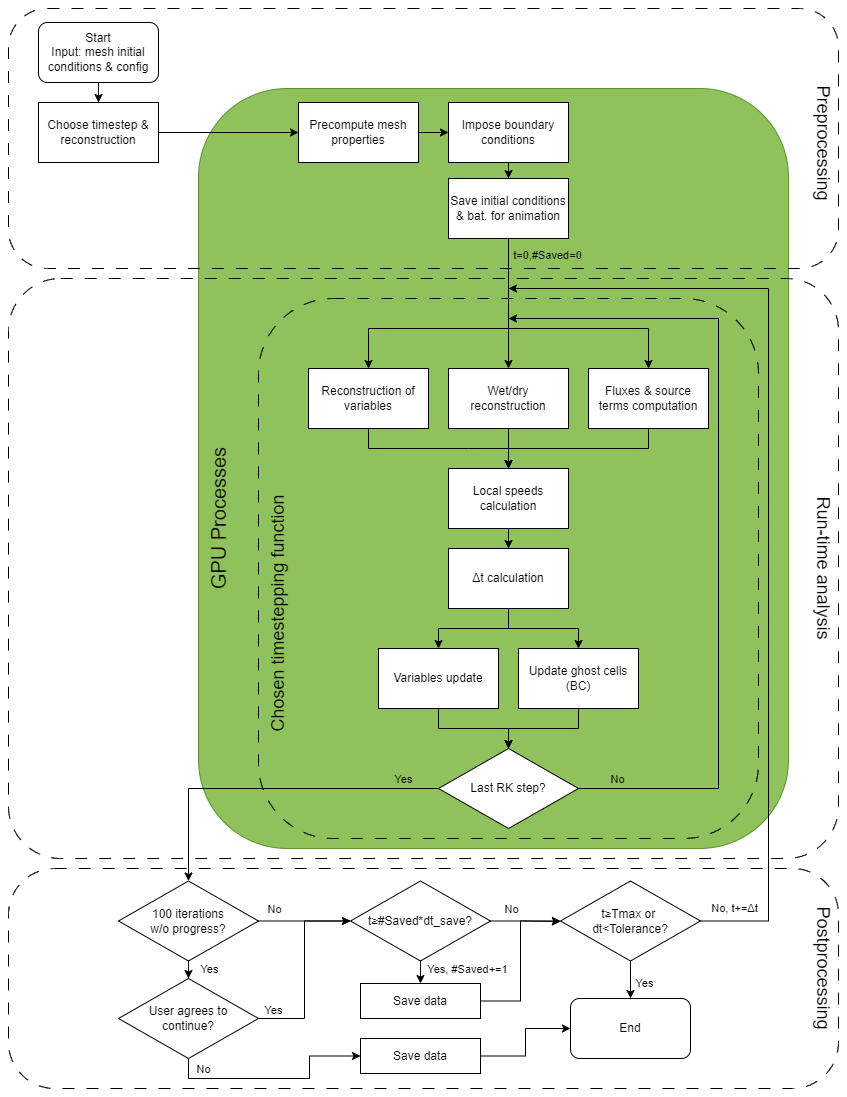
Figure 5 Overview of the SWEpy software parallel structure and architecture. The green box contains tasks performed on the GPU. The innermost segmented box contains tasks done by the chosen timestepping method. Outer segmented boxes indicate phases. Postprocessing phase highlights stagnation and divergence detection, and user controlled data saving. Arrows going into/out of green box indicate CPU-GPU synchronization. We highlight that the figure provides a high-level overview of module organization and data flow, rather than a function-level representation of the code structure.

4.1 Preprocessing

4.1.1 Loading input data (FileLoader.load_from_files)

As shown in the upper portion of Fig. 5, the preprocessing phase initializes the simulation by organizing all input data for efficient GPU execution, reducing subsequent CPU–GPU transfers and enabling scalability on large unstructured grids.

SWEpy takes as input a user-defined triangular mesh – specified through vertex coordinates, connectivity, and bathymetry values – along with initial conditions for the conserved variables, boundary ghost-cell definitions, and a configuration file containing simulation parameters (e.g., numerical tolerances, final time, gravitational acceleration, CFL number, and optional source-term coefficients such as Manning roughness or Coriolis effects).

All inputs are consolidated into the mesh dictionary, which serves as the central data structure throughout the simulation.

4.1.2 Bathymetry generation (Utilities.bathymetry_midpoint/2)

Bathymetry is reconstructed using an interpolator consistent with the chosen spatial reconstruction. For instance, a linear interpolator is employed with the minmod scheme (Bryson et al., 2011). This process involves interpolating vertex values to both edge Gaussian points and the cell interiors, which are required for source term evaluations in Eq. (20).

The interpolation relies on simple algebraic operations (such as computing the gradient of a plane defined by the three vertices of each triangle) and is vectorized for efficient execution on the GPU. Relevant quantities are precomputed and stored to further enhance performance.

4.1.3 Geometric computations on the mesh (FileLoader.compute_element_properties)

Key geometric properties required by the numerical scheme, such as cell areas $\left|{\mathrm{\Omega }}_j\right|$, edge lengths l_jk, barycenters (x_j,y_j), perpendicular heights r_jk, and second area moments $I_x,I_y,I_{xy}$ (Utilities.second_moments; see Fuenzalida Alarcón et al., 2025), are computed in parallel for all cells.

Using CuPy’s vectorized array operations, these quantities are evaluated directly from vertex coordinates, enabling simultaneous computation across the entire grid on the GPU. This approach significantly accelerates the preprocessing stage, particularly for the high-resolution meshes typical of flood and tsunami simulations.

4.1.4 Stencil generation for high-order reconstruction (Utilities.precomp_weno2)

For quadratic WENO reconstruction, a vectorized procedure identifies first- and second-order neighbors in a single time, while flagging boundary cells with incomplete stencils for fallback to the minmod scheme. The least-squares matrices (right-hand side of Eq. A2), which depend only on grid geometry, are precomputed using CuPy’s linalg routines. Matrix inversions and multiplications are performed in parallel over stacked systems, and the resulting coefficients are stored as arrays for efficient reuse during the run-analysis phase.

By shifting these computations to the GPU and avoiding repeated stencil assembly, the preprocessing establishes a data-parallel foundation, enabling SWEpy to handle complex simulations with minimized runtime delays.

4.2 Run-analysis (ShallowWater.run/run_with_TS)

The run-analysis phase – depicted by the central segmented box in Fig. 5 – forms the core of SWEpy's time integration. In this stage, the solution is advanced iteratively through spatial reconstruction, source-term evaluation, flux computation, and state updates, all implemented to exploit GPU parallelism. By leveraging CuPy’s array-based operations, these calculations are performed concurrently across the entire mesh, minimizing serial bottlenecks and enabling efficient simulation of large-scale flows, such as those presented in Sect. 5.

Prior to entering the main time-stepping loop, the program chooses the “timestep” function to be used according to user selection (ShallowWater.choose_timestep). This timestep function is central as it defines the sequence of operations performed at each iteration – including reconstruction, flux evaluation, and source-term treatment – consistent with the CU formulation and the chosen temporal discretization. In essence, it encapsulates the definition of a single update step.

This design provides flexibility: by modifying or extending the timestep routines using the components described below, users can readily switch between reconstruction strategies, source-term models, time integration schemes, and even flux definitions.

4.2.1 Reconstruction (PieceWiseReconstruction.minmod/weno2)

For minmod reconstruction, SWEpy evaluates cell-centered gradients using neighboring average states and reconstructs the conserved variables q_j(M_jk) at edge midpoints for flux computations in Eq. (16). Water surface values are also reconstructed at vertices to support wet/dry treatment. An optional diffusion parameter, $\mathit{\vartheta }\in [\mathrm{1},\mathrm{2}]$ (cf. Eq. 26, can be specified to control numerical dissipation: larger values reduce diffusion but may increase the risk of spurious oscillations.

All gradient evaluations and interpolations are implemented using CuPy’s vectorized operations, exploiting SIMD parallelism to process all cells simultaneously on the GPU. As a result, the sequential loops described in Algorithm A1 are effectively replaced by fully parallel array-based computations, significantly improving performance.

For WENO reconstruction, SWEpy solves the LSQ linear systems in Eq. (A2) using precomputed matrices to obtain the reconstruction polynomials. These polynomials are then evaluated at the required quadrature points: edge Gaussian points for flux computations in Eq. (16), interior Gaussian points for source-term evaluation in Eq. (20), and cell vertices for wet/dry treatment.

Because the reconstruction stencils are preassembled during preprocessing, all evaluations can be carried out simultaneously across the mesh using GPU-accelerated operations. Consequently, the cell-wise iterations described in Algorithm A2 are fully vectorized and executed in parallel, significantly enhancing computational efficiency.

Boundary cells lacking full second-order neighbors, identified during preprocessing, default to minmod reconstruction. Wet/dry fronts are corrected by replacing invalid reconstructions (negative depths) using CuPy's fancy indexing to locate and adjust affected cells in parallel, executing Algorithm A3 via SIMD commands on the GPU without explicit loops. This means that “for-loops” in Algorithm A3 are replaced by SIMD commands for all cells, efficiently performed over the GPU.

The modular design of SWEpy further allows users to define custom reconstruction operators, provided they supply interpolated values at the required points. This facilitates extensions – such as hybrid reconstruction strategies – while maintaining GPU efficiency.

4.2.2 Source Terms (CentralUpwindMethod.source_term/2, coriolis, friction_term)

Bathymetry source terms are evaluated in all cells using Eq. (20), based on the precomputed bathymetry reconstruction and the selected spatial operator. Additional contributions, such as Coriolis and friction terms, are computed from the cell states and stored for use during the update step.

All source-term evaluations are fully vectorized and executed on the GPU, ensuring efficient parallel computation, including for optional physics. The modular framework also allows users to incorporate additional source-term models, provided they remain consistent with the chosen spatial discretization, reconstruction strategy, and time-integration scheme.

4.2.3 Local speeds and time steps (CentralUpwindMethod.one_sided_speed/2)

Using the reconstructed states, velocities are desingularized and projected onto edge normals to evaluate the local propagation speeds in Eq. (19). These computations are performed simultaneously for all edges using GPU-parallel operations. When adaptive time stepping is enabled, the time increment Δt is determined from the CFL stability condition based on the computed wave speeds, maximizing the allowable step size to improve efficiency while limiting numerical diffusion (cf. Eq. 31).

Explicit Euler (EE) integration applies Eq. (16) through fully vectorized GPU operations, with CPU synchronization limited to advancing the timestep (one cycle in Fig. 5). The SSP RK(4,3) scheme (Gottlieb et al., 2010) and the classical four-stage RK4 method are implemented as sequences of scaled explicit Euler updates. These stages are executed sequentially on the GPU, avoiding iterative solvers and minimizing overhead, with optional friction corrections applied at each stage.

The modular design of the timestep function allows user-defined integration schemes to be seamlessly incorporated into the GPU workflow. This enables future extensions, such as predictor–corrector methods or modified Newton–Raphson iterations for implicit formulations, although the latter remain less suited to efficient GPU execution.

4.2.4 Variable update and correction (timestep function)

Fluxes are assembled from the reconstructed states and local wave speeds, and the cell averages are updated according to the CU scheme in Eq. (16) through a single GPU-parallel operation, followed by the enforcement of ghost-cell boundary conditions. For Manning friction, an intermediate semi-implicit correction is applied to the discharge, performed vector-wise across the grid.

In multi-stage RK schemes, intermediate states and fluxes are computed and stored on the GPU, with optional friction corrections applied at each stage. This design minimizes CPU–GPU synchronization while preserving the intended order of accuracy as represented in Table 2.

4.2.5 Boundary conditions (BoundaryConditions.impose)

The program enforces user-defined boundary conditions through the ghost cell states. Because each ghost cell is independent, mixed boundary conditions along domain boundaries can be applied simultaneously. The modular structure of the code further supports the implementation of more advanced boundary treatments, such as transport-based models for coupling with external solvers, commonly referred to as sequential or iterative coupling.

The boundary conditions currently implemented through ghost cells include: (a) a zero-order extrapolation permeable (soft) boundary, in which the border cell state is replicated in the adjacent ghost cell; and (b) an impermeable (wall) boundary, where the water height is replicated while the flow direction is reversed, effectively reflecting the flux and enforcing a zero-normal-flow condition at the interface.

We note that periodic boundary conditions can be incorporated by defining boundary cells as neighbors of other boundary cells. For example, to impose periodicity between the top and bottom boundaries of a channel, the bottom cells are treated as the upward neighbors of the top boundary cells, and vice versa. This approach is used in several of our experiments. Please refer to the User Manual & Technical Reference (Meza et al., 2026) for details.

4.3 Postprocessing (FileSaver module)

The post-processing phase, illustrated in the lower portion of Fig. 5, concludes the simulation by handling data output and termination criteria. Leveraging the modular design of SWEpy, this stage supports customizable workflows tailored to both research analysis and operational monitoring. Users can integrate predefined or custom routines to export results at any point during runtime, enabling both real-time inspection and efficient post-simulation analysis.

For data storage, SWEpy provides built-in functionality to save initial conditions and bathymetry (FileSaver.save_bathymetry) in .vtk format prior to the simulation, followed by solution snapshots at user-defined intervals Δt_save throughout the run (FileSaver.save_animation). This format is optimized for visualization tools such as ParaView (Ayachit, 2015), allowing users to render both static fields and time-resolved animations over unstructured grids. In addition, time series data at selected locations (e.g., virtual gauges for tsunami validation; see Sect. 5) can be recorded at the same Δt_save (FileSaver.save_TS). Because these routines are integrated directly into the runtime, they enable continuous monitoring of the evolving solution – an important feature for identifying anomalies in long simulations without interrupting execution. Efficient data handling is ensured through CuPy’s GPU-compatible NumPy routines (e.g., save, savez, savetxt), which allow high-frequency output with minimal performance overhead.

By default, the simulation terminates once the prescribed final time is reached. However, the modular framework allows for additional user-defined stopping criteria, such as divergence detection (e.g., when an adaptive Δt falls below a threshold) or stagnation monitoring (e.g., negligible state evolution over a specified number of iterations). These criteria can be implemented by extending or modifying the run functions. In our experiments, such controls proved effective in preventing unproductive simulations and complemented the live visualization capabilities for real-time decision-making. More broadly, this flexibility enhances SWEpy's applicability, enabling integration with external tools for automated error handling or real-time coupling in hybrid modeling workflows.

5 Results and Discussion

This section presents a series of numerical experiments to validate SWEpy's implementation, accuracy, and performance against analytical benchmarks and real-world cases, demonstrating the effectiveness of the CU scheme with WENO reconstructions and GPU acceleration as described in Sects. 3 and 4. We begin with canonical tests that assess spatial and temporal accuracy, well-balancing, positivity preservation, and numerical diffusion reduction, followed by synthetic scenarios that highlight the versatility of the reconstruction operators. Finally, large-scale simulations of the 1959 Malpasset dam failure and the 2010 Maule tsunami assess real-world applicability by comparing results with historical data and established solvers such as TELEMAC (Moulinec et al., 2011). These experiments underscore SWEpy's robustness for inundation modeling over complex topography and long-range wave propagation, achieving high-resolution outcomes on consumer hardware with computation times reduced by factors of up to 21× via CuPy parallelism.

5.1 Benchmark tests

5.1.1 Spatial convergence order study

To validate SWEpy's spatial accuracy and verify the correct discretization of the bathymetry source term (Eq. 20), we replicate the convergence test of Bryson et al. (2011), focusing on scenarios where well-balancing is critical to preserve steady states over non-flat topography free of spurious oscillations. The test quantifies the order of convergence for different spatial reconstruction operators (Sect. 3.3) over a smooth Gaussian bump.

The computational domain is a 2×1 m rectangle discretized into a regular mesh of equilateral triangles, where triangles along the top and bottom boundaries are halved to ensure consistent boundary treatment. The bottom topography is defined as

$$\begin{array}{}\text{(32)}& B(x,y)=\mathrm{0.5}\exp (-\mathrm{25}(x-\mathrm{1}{)}^{\mathrm{2}}-\mathrm{50}(y-\mathrm{0.5}{)}^{\mathrm{2}}).\end{array}$$

The initial conditions consist of a uniform free-surface elevation $w(x,y,\mathrm{0})=\mathrm{1.0}\mathrm{m}$ and a velocity field $u(x,y,\mathrm{0})=\mathrm{0.3}$ m s⁻¹, $v(x,y,\mathrm{0})=\mathrm{0}$ m s⁻¹. Fully permeable (zero-gradient) boundary conditions are applied on all sides, with g=1 m s⁻². The flow evolves to a steady, non-uniform state by t≈0.07 s, at which point temporal errors become negligible and spatial errors dominate.

The reference solution is computed on a fine grid with n_x=512 horizontal divisions (approximately 1.18×10⁶ cells) at t=0.07 s. Figure 6 illustrates the Gaussian bump on a coarse grid (n_x=32) and the corresponding reference solution. The L² error is defined as

$$\Vert e{\Vert }_{\mathrm{2}}=\sqrt{\sum _j\left|{\mathrm{\Omega }}_j\right|({\stackrel{\mathrm{‾}}{w}}_j-w_{\mathrm{ref},j}{)}^{\mathrm{2}}},$$

Convergence orders are then estimated via successive grid refinements. Table 2 reports errors and orders for grids p=0 to 3 ($n_x=\mathrm{32}\cdot {\mathrm{2}}^p$) across combinations of reconstruction operator and time-stepping scheme, while Fig. 7 shows the log–log relationship between error and effective grid spacing Δx, with fitted power laws consistent with the expected convergence rates.

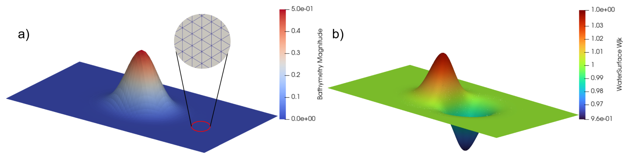
Figure 6 Bottom topography on a n_x=32 point grid (left) and reference solution (right) for the Gauss bump. The zoomed-in circular window highlights the grid structure pattern.

Table 2 L² errors and numerical orders of accuracy. Grid number p corresponds to $nx=\mathrm{32}\cdot {\mathrm{2}}^p$ horizontal divisions of the domain.

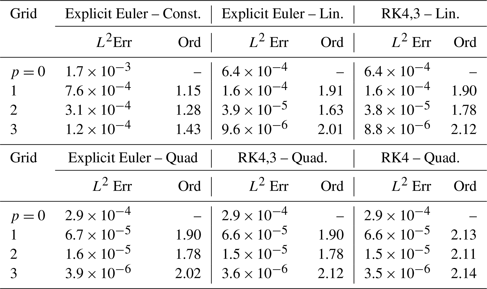
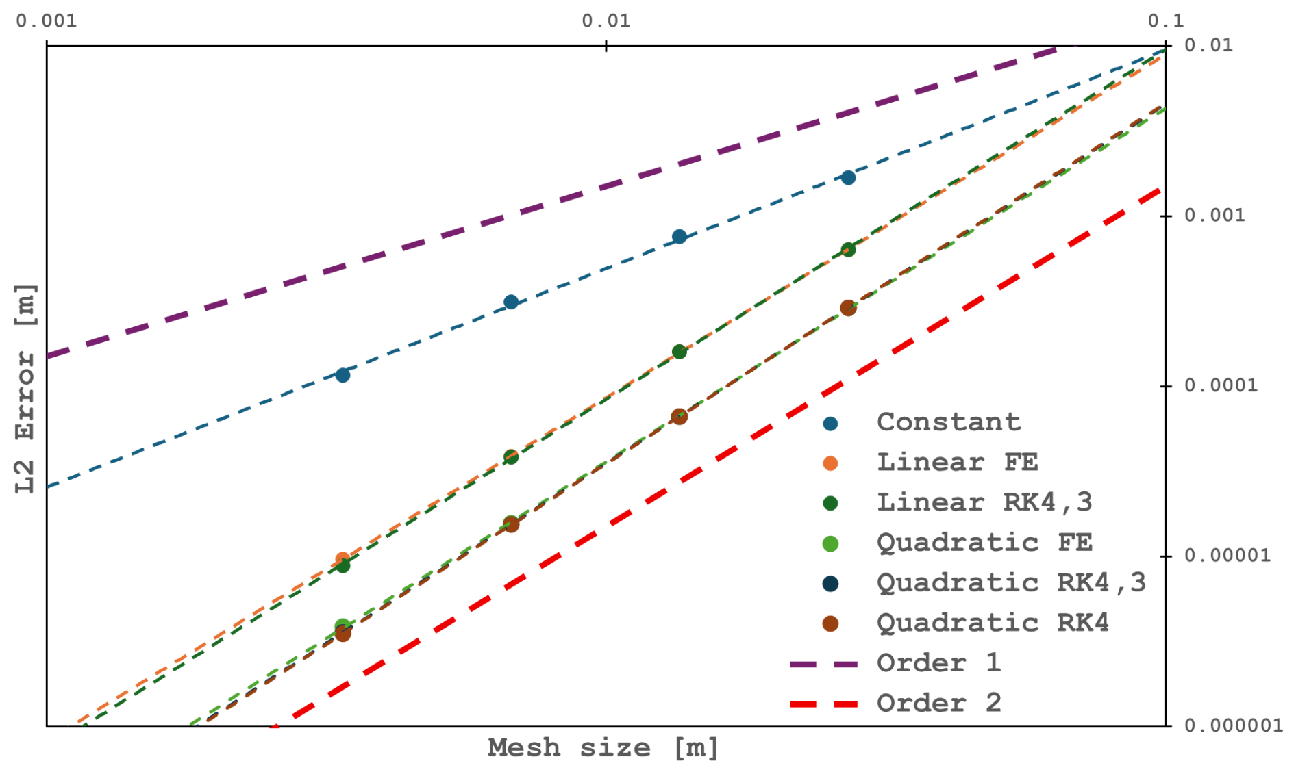
Figure 7 Log-log plot of L² error versus grid size Δx, with fitted power-law curves indicating convergence orders.

The results confirm the robustness of all configurations. Constant reconstruction yields better-than-first-order accuracy, while linear and quadratic reconstructions approach second-order convergence, in agreement with the scheme’s formal order for smooth solutions.

The theoretically attainable third-order accuracy with quadratic reconstruction is not achieved, suggesting that further refinement of either the numerical flux formulation or the bathymetry source term discretization may be needed to fully realize higher-degree polynomial benefits. This order degradation is an expected behavior, also reported by Bryson et al. (2011), and more recently by Nguyen (2023). However, a detailed convergence analysis of the extended scheme is beyond the scope of this work. Nevertheless, WENO-based quadratic reconstruction consistently produces the smallest errors, outperforming lower-order approaches across all resolutions. This improved accuracy is particularly relevant in precision-critical scenarios, where error propagation over long timescales can be significant.

From a practical performance standpoint, generating the fine-grid reference solution with explicit Euler time-stepping and linear reconstruction required approximately 5 min wall-clock time on consumer-grade GPU hardware, including output at a high-frequency interval of 0.01 s for animation purposes. This demonstrates that SWEpy can deliver high-resolution, well-balanced solutions for flows over smooth-bottom at modest computational cost.

5.1.2 Well-balancing test

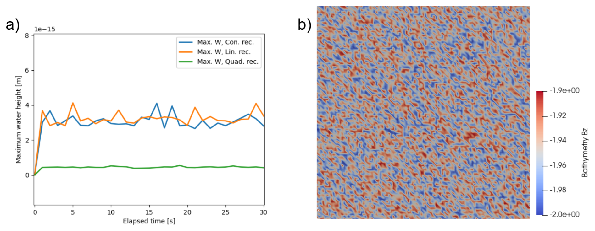
We simulate a static flat water surface over white-noise-generated bathymetry to verify the well-balanced property for all reconstruction operators. The domain is a 1×1 m² domain, with a random bathymetry with mean depth of d=2, uniformly distributed in $[-\mathrm{1.1}d;-\mathrm{0.9}d]$, discretized using a right-triangles mesh with $\mathrm{\Delta }x=\mathrm{\Delta }y=\mathrm{0.01}$. The dry tolerance is set to 10⁻¹⁷ to assess machine-precision accuracy. Simulations use explicit Euler time-stepping with an adaptive timestep and CFL =0.25.

The initial water surface is set to 0 m and the velocity field is set to zero in both directions. Figure 8 shows the random bathymetry and the maximum water height over time for the three reconstructions, confirming that no spurious oscillations arise. These results, while potentially surprising, are in fact expected since the bathymetry source term discretization is exactly well balanced by construction. This means that even in the presence of boundary conditions, unphysical oscillations or flows will not appear. Notably, this experiment also confirms the well-balancing property with the Runge Kutta scheme, since it is implemented as four successive explicit Euler steps.

Figure 8 (a) Maximum water height over time. (b) Randomly generated bathymetry.

5.1.3 Conical island wetting–drying benchmark

To evaluate SWEpy's wet/dry handling and reconstruction performance during wave-obstacle interactions, which are essential for coastal inundation modeling, we simulate the conical island benchmark, a laboratory experiment (Briggs et al., 1995) widely used for SWE validation (Synolakis et al., 2008). This test assesses (i) positivity preservation on sloped topography, where runup/rundown induces dynamic wetting without unphysical negative water depths, and (ii) operator fidelity in capturing complex wavefronts. The domain is a 41×30 m tank with permeable (soft) boundaries to absorb reflections, thereby minimizing boundary artifacts. The domain is discretized using an equilateral triangular mesh with edge length 0.5 m (approximately 12 000 cells) , ensuring spatial isotropy. The bathymetry consists of a flat bottom with a truncated cone (base diameter 7.2 m, crest diameter 2.2 m, height 0.625 m) centered at the origin, simulating an island. The initial free-surface elevation is given by the solitary-wave profile:

$$\begin{array}{}\text{(33)}& w(x,y,\mathrm{0})={\displaystyle \frac{H}{d}}{\mathrm{sech}}^{\mathrm{2}}\left(\mathit{\gamma }\right(x-X_{\mathrm{1}}\left)\right),\end{array}$$

with d=0.320 m, H=0.02976 m, and $\mathit{\gamma }=\sqrt{\mathrm{3}H/\mathrm{4}{d}^{\mathrm{3}}}$, positioned at $X_{\mathrm{1}}=-\mathrm{13}\mathrm{m}$. The initial velocity field is

$$\begin{array}{}\text{(34)}& \begin{array}{rl}& u(x,y,\mathrm{0})={\displaystyle \frac{g}{d}}w(x,y,\mathrm{0})\left(\mathrm{1}-\mathrm{0.25}{\displaystyle \frac{w(x,y,\mathrm{0})}{d}}\right),\\ & v(x,y,\mathrm{0})=\mathrm{0},\end{array}\end{array}$$

The initial condition is derived to ensure consistent propagation and extruded uniformly in the y-direction to simulate a two-dimensional wave front. Simulations are conducted with constant, minmod, and WENO reconstruction operators for cross-comparison, employing an explicit Euler time integration scheme with a Courant-Friedrichs-Lewy (CFL) number of 0.25. The reason for this temporal integration setup is twofold: (1) it demonstrates the solver's capability to operate at higher effective CFL numbers, and (2) it is sufficiently low to keep oscillations controlled, thereby isolating spatial-reconstruction effects and enabling a focused assessment of how each operator handles wet/dry transitions and wavefront modeling as the soliton interacts with the cone, as shown in the initial setup of Fig. 9.

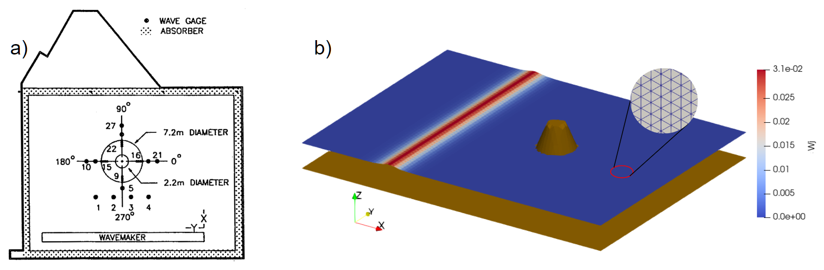
Figure 9 (a) Configuration of original experiment (digitized from Briggs et al., 1995) for the conical island benchmark. (b) 3D view illustrating the solitary wave profile approaching the truncated cone.

Figure 10 shows the free-surface elevation at each computational element (W_j) for each reconstruction operator at t=7 s, as the leading wave passes gauge 16. This snapshot provides a spatial context for the subsequent time-series comparison, highlighting differences in wavefront sharpness and height at the gauge location. The WENO reconstruction yields the sharpest and highest wave at gauge 16 (η≈0.041 m), the minmod reconstruction shows moderate attenuation (η≈0.03 m), and the constant reconstruction produces a visibly diffused wavefront (η≈0.011 m). Green markers indicate the positions of gauges 1, 6, 16, and 22 (from left to right), consistent with the original experimental layout for direct validation of runup dynamics.

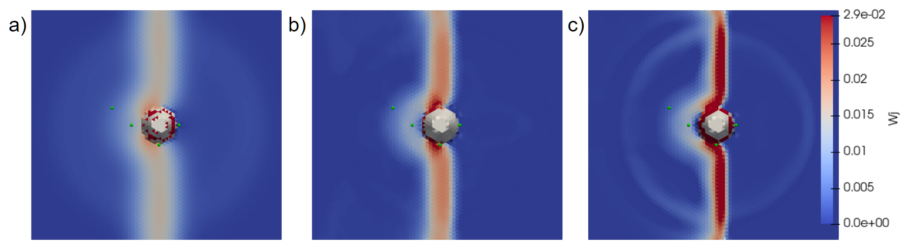
Figure 10 Comparison of wave structure while passing through gauge 16. Free-surface elevation at t=7 s for (a) constant, (b) minmod, and (c) WENO reconstruction operators. Green markers indicate the positions of gauges 1, 6, 16, and 22 (from left to right).

We note that, due to the nature of the wet/dry reconstruction procedure, minimal numerical artifacts arise near the wet/dry interface in the form of “wet” triangles with very small water column heights (approximately 10⁻⁵–10⁻⁴ m). This effect can be further mitigated by adjusting the dry tolerance parameter in the simulation configuration file or by grid refinement, as shown in Fig. 11: The numerical artefacts are significantly reduced in the finer grid, with water column heights near the interface of order 10⁻¹⁰–10⁻⁹ m.

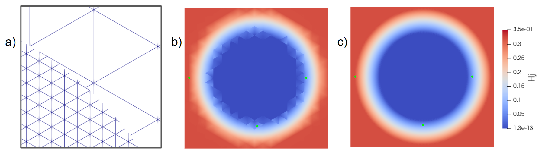
Figure 11 (a) Grid size comparison closeup. Water column heights (Hj) around protrusion of conical island diminish from the (b) coarse grid to the (c) fine grid.

Figure 12 presents time-series of water surface elevation for gauges 1, 6, 16, and 22 using the constant, minmod, and WENO reconstruction operators. The laboratory records, originally timed from wavemaker initiation, have been shifted by −25 s to align the incident wave arrival time with simulations. This value corresponds to the estimated paddle deceleration inferred from signal traces in Briggs et al. (1995).

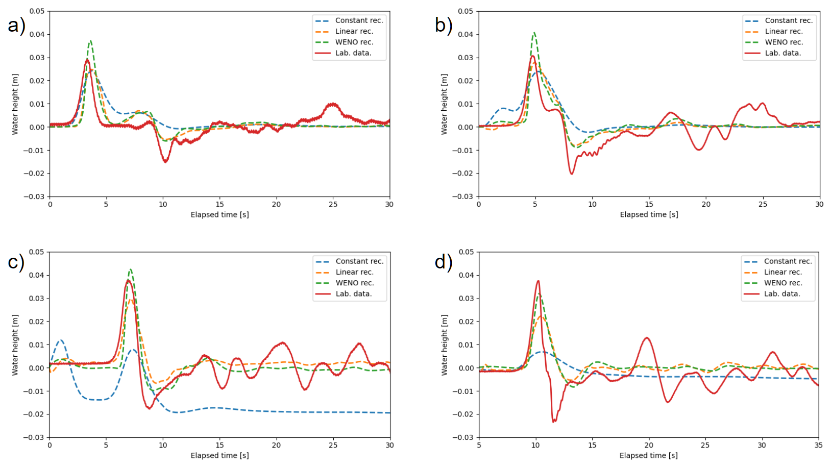
Figure 12 Time series of water heights at gauges 1 (a), 6 (b), 16 (c), and 22 (d). Solid line is laboratory data, and dashed lines are SWEpy's solutions.

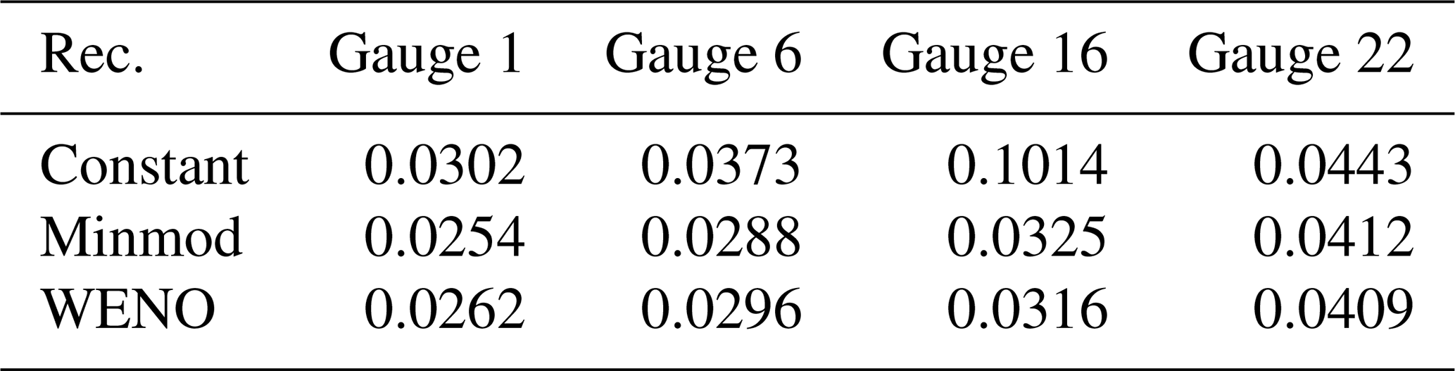
Across gauges, WENO accurately reproduces main crest height and arrival time with minimal phase error, while constant and minmod underestimate secondary oscillations and exhibit greater dissipation during rundown. Quantitatively, the L² norm of differences between numerical and experimental series (Table 3) confirms that WENO and minmod exhibit similar performance, with WENO showing slightly higher averaged errors over the four gauges (${\stackrel{\mathrm{‾}}{\left|e\right|}}_{\mathrm{2}}^{\text{WENO}}=\mathrm{0.0321}$ vs. ${\stackrel{\mathrm{‾}}{\left|e\right|}}_{\mathrm{2}}^{\text{minmod}}=\mathrm{0.0320}$), while both outperform constant by approximately 40 % (${\stackrel{\mathrm{‾}}{\left|e\right|}}_{\mathrm{2}}^{\text{constant}}=\mathrm{0.0533}$).

Table 3 L² error of time series for each reconstructor at the different gauges.

Since L² is phase-sensitive and the phase shift cannot be determined exactly, we repeated the analysis by applying uniform shifts from −0.10 to +0.30 s to the numerical series (Table 4). Across all tested shifts, WENO consistently achieved the lowest error scores, confirming its robustness to phase uncertainty and its suitability for dynamic wetting–drying reconstruction in coastal flows.

Table 4 L² average error for each reconstructor with different time shifts of laboratory data to account for phase error.

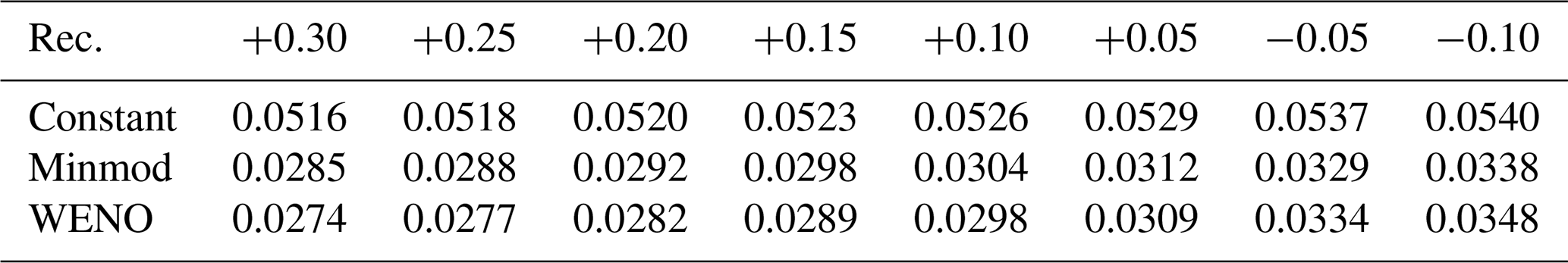
Figure 13 illustrates spatial diffusion effects by comparing the free-surface elevation at t=13 s across the three reconstruction operators, at a stage where the wave has traversed the island and formed the cardioid-shaped crest pattern observed in laboratory measurements. The WENO reconstruction (panel c) preserves sharp gradients, with minimal attenuation and good retention of intricate structures. By contrast, the minmod reconstruction (panel b) maintains the overall pattern but introduces noticeable smoothing, while the constant reconstruction (panel a) dissipates most fine-scale features, resulting in a blurred profile. To quantify these differences, we computed the depth-integrated potential energy $\mathcal{E}=\mathit{\rho }g{\int }_{{\mathrm{\Omega }}_{\mathrm{strip}}}{\mathit{\eta }}^{\mathrm{2}},\mathrm{d}\mathrm{\Omega }$ over a vertical strip from x_l=9.5 m to x_r=14.5 m downstream, where η=w since the still-water level is zero in the solitary-wave setup. The energies are ℰ_const=0.015, ℰ_minmod=0.020, and ℰ_WENO=0.044, confirming WENO's superior wave energy retention in the post-interaction field. Combined with the L² analysis, these findings underscore WENO's superior balance between low numerical diffusion and faithful waveform reproduction, whereas the constant reconstruction underperforms in both aspects.

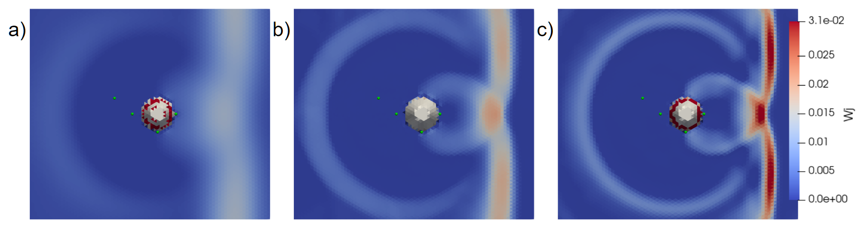
Figure 13 Diffusion study. Solution at time t=13 s for constant (a), linear (b), and quadratic (c) reconstructors. Green marks are the locations of gauges 1, 6, 16, and 22 (from left to right).

In this work, we use the energy-based measure ℰ to quantify the extent of numerical diffusion. This metric, together with the comparisons at measurement stations, provides sufficient evidence to support the conclusions regarding WENO's superior performance in capturing wave dynamics. As noted above, point measurements capture only one aspect of the numerical result, being useful for specific events such as wavefront arrival time, zones of maximum amplitudes, or inundation extent, among others. In addition, Fig. 13 shows a plan view to emphasize the importance of a global approach to the numerical results and their relation to the physical problem analyzed.

In that direction, and building on the finding that the WENO-based approach captures relevant information for global analysis, Fig. 14 provides a detailed sequence of the wavefront evolution under WENO reconstruction, illustrating how it maintains sharp gradients and structural integrity throughout the interaction at t=7, 8, and 9 s. The leading crest propagates toward the island, splits, and wraps around its flanks, producing a clear diffraction pattern. In the lee, the opposing wavefronts converge and form a coherent cusp that advances shoreward. A small, nearly circular secondary wave is visible behind the main crest; this is a residual artifact of the wetting–drying correction process, but it decays rapidly and does not trigger further spurious oscillations. For the whole simulation, the shoreline evolves smoothly, and the wavefront retains sharp gradients throughout the interaction, even in the presence of zeroth-order boundary conditions. Thus, the wavefront sequence in Fig. 14 illustrates that SWEpy's implementation incorporates the appropriate numerical foundations, enabling detailed descriptions of more complex real-world phenomena.

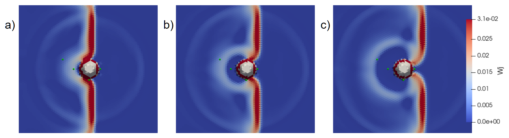
Figure 14 Wave-obstacle interaction study. Solution at times t=7 s (a), t=8 s (b), and t=9 s (c), using the WENO reconstruction operator. Green marks are the locations of gauges 1, 6, 16, and 22 (from left to right).

Overall, the conical-island benchmark confirms that SWEpy reproduces the key hydrodynamic processes involved in wave–obstacle interaction, including runup and rundown on sloping topography, diffraction around an emergent feature, and convergence in the lee. The comparison with laboratory measurements demonstrates that the WENO reconstruction consistently achieves the most faithful representation of surface elevation amplitude, phase, and post-interaction structure, while maintaining stability at wetting–drying fronts, and ensuring positivity preservation. Although small discrepancies remain–particularly in negative water levels following the first rundown–these can be attributed to physical processes not represented in the depth-averaged SWE framework (e.g., vertical accelerations) and to uncertainties in the temporal alignment between the laboratory and numerical time series. Taken together with the other validation cases, these results highlight the model’s capability to resolve complex nearshore hydrodynamics with high numerical fidelity, especially when paired with high-order reconstruction.

5.1.4 Computational Performance and Scalability

To assess SWEpy's computational efficiency, we performed scaling benchmarks from coarse to fine resolutions using the Conical Island and Gaussian Bump test cases introduced previously. Table 5 summarizes execution times on an NVIDIA GeForce GTX 1650 GPU versus a serial single-core CPU implementation on an Intel Core i5-10300H.

Table 5 Average execution time per time-step for idealized benchmarks (NVIDIA GTX 1650 vs. Serial Intel Core i5-10300H CPU). Speedups are relative to the single-core CPU baseline.

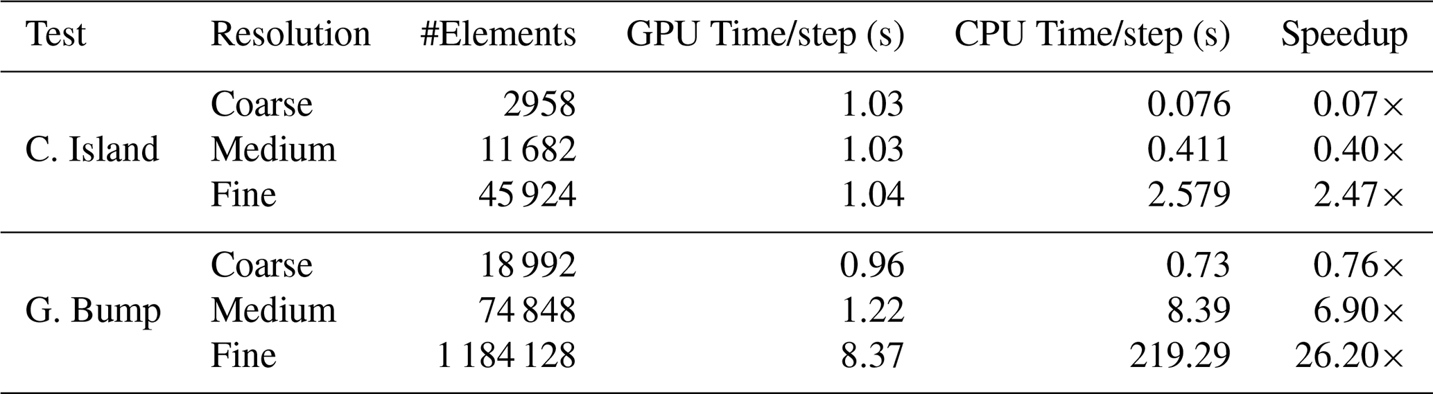
The results illustrate a characteristic performance transition between latency-bound and throughput-bound regimes typical of GPU-accelerated frameworks. For small meshes (e.g., Conical Island coarse, ∼ 3000 elements), the GPU execution time is dominated by fixed overheads–kernel launch latencies and host-device synchronization–resulting in negligible or even fractional speedups relative to the CPU. In this regime, the serial CPU implementation is competitive due to its lack of launch overhead.

However, scaling behavior improves dramatically with problem size. As the element count increases, the massive parallelism of the GPU is more effectively utilized. In the Gaussian Bump case with ∼ 1.2 million elements, the solver transitions into a throughput-bound regime, achieving a speedup of 26.2×. This confirms that SWEpy's architecture is well-suited for high-resolution scenarios where the arithmetic intensity of WENO reconstruction saturates the GPU's CUDA cores.

It is worth noting that, to maintain a fair comparison with respect to code structure and accessibility, the CPU implementation was developed as a direct port of the GPU version. This design choice results in worse-than-linear time scaling with problem size, as seen in Table 5, and has two primary causes. First, both implementations follow a deliberately straightforward computational structure to preserve user accessibility. Second, the wet/dry algorithm relies on comparison and indexing operations (np.where, np.count_nonzero, and fancy indexing) over arrays that may not be in contiguous memory layout due to transposition and stacking; resolving this would require restructuring the code in ways that would break the structural similarity between the CPU and GPU versions, making the comparison less fair. As a consequence, the reported speedup values should be interpreted with care: they reflect the advantage of the GPU implementation over this specific unoptimized serial baseline.

Furthermore, system traces reveal the hardware utilization patterns across different scales. As shown in Table 6, GPU throughput – measured as SM occupancy, i.e., the average percentage of warps active in streaming multiprocessors during runtime – rises from 22.9 % at coarse resolution to 91.1 % at fine resolution in the Gaussian Bump benchmark, confirming effective saturation of the computing resources. In the Conical Island case, however, the wetting–drying correction procedure combined with the extended simulation duration significantly increases the number of GPU kernel launches without a proportional gain in throughput. This indicates that the high density of kernel launches throttles the efficient use of computational resources, suggesting that CuPy optimizations such as kernel fusion or element-wise kernels for arithmetic-intensive operations could substantially improve performance.

Table 6 GPU performance metrics derived from system traces for the Conical Island and Gaussian Bump benchmarks.

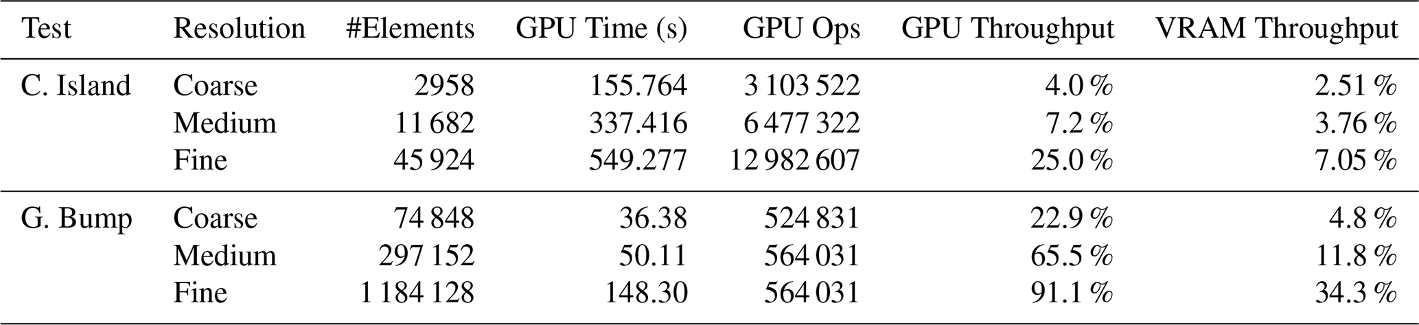
In terms of memory usage, the software exhibits a predictable VRAM utilization behavior, measured as the ratio of allocated to total available memory, that increases with mesh size. However, memory usage does not depend exclusively on mesh size. As shown in Table 6, the fine-resolution Conical Island grid has fewer elements than the coarse Gaussian Bump grid, yet exhibits higher memory utilization, owing to the additional memory demands of the active wetting-drying handling algorithm.

In addition, we quantified the cost of adaptive time-stepping. Profiling on the finest mesh showed that computing the adaptive Δt accounts for approximately 3 % of the total runtime (3.85 s out of 142.1 s total for the Gaussian bump run). In contrast, imposing a fixed conservative time-step to ensure stability increased the total runtime to 148.3 s. Thus, the computational overhead of adaptive time-step control is negligible compared to the efficiency gains from maximizing the stable time-step size.

The performance analysis presented in this subsection characterizes how solver efficiency varies with problem size on a fixed single-GPU device. Unlike formal strong or weak scaling studies, which assess performance as the number of processing units or available memory varies, this analysis captures the transition from latency-bound to throughput-bound execution as the workload grows to saturate the available hardware. A multi-device scaling study remains an important avenue for future work.

5.2 Real-life scenario 1: Malpasset Dam failure

To evaluate SWEpy’s performance in realistic inundation scenarios involving complex topography and moving wet/dry fronts, we reproduce the 1959 Malpasset dam failure on France’s Reyran River. The event is characterized by rapid flooding over highly irregular terrain (Moulinec et al., 2011). This case is used to validate the model’s positivity-preserving reconstruction schemes, treatment of bathymetric source terms, and semi-implicit friction formulation described in Sect. 3.

The computational domain is discretized using an unstructured triangular grid adapted from the TELEMAC-2D validation dataset. The mesh contains 26 000 elements, with characteristic triangle heights Δr (measured from a vertex to the opposing side) ranging from 4.01 to 401.95 m, and an average value of 40.28 m.

The bathymetric and topographic data are derived from the 1931 IGN Saint-Tropez map, with additional refinement upstream of the dam to better resolve steep gradients (Fig. 15a, inset). The initial condition sets the reservoir water surface to an elevation of 100 m upstream of the dam, represented as a vertical plane between coordinates (4701.18, 4143.10) and (4655.50, 4392.10), and 0 m elsewhere, with all cells above sea level initialized as dry (Fig. 15b). Boundary conditions are specified as impermeable walls, consistent with the TELEMAC reference configuration. The Manning roughness coefficient is set to n=0.03 to match the TELEMAC reference setup. The simulation employs minmod reconstruction and adaptive time-stepping with a Courant–Friedrichs–Lewy (CFL) number of 0.33, and is run until $t_{max}=\mathrm{4000}$ s.

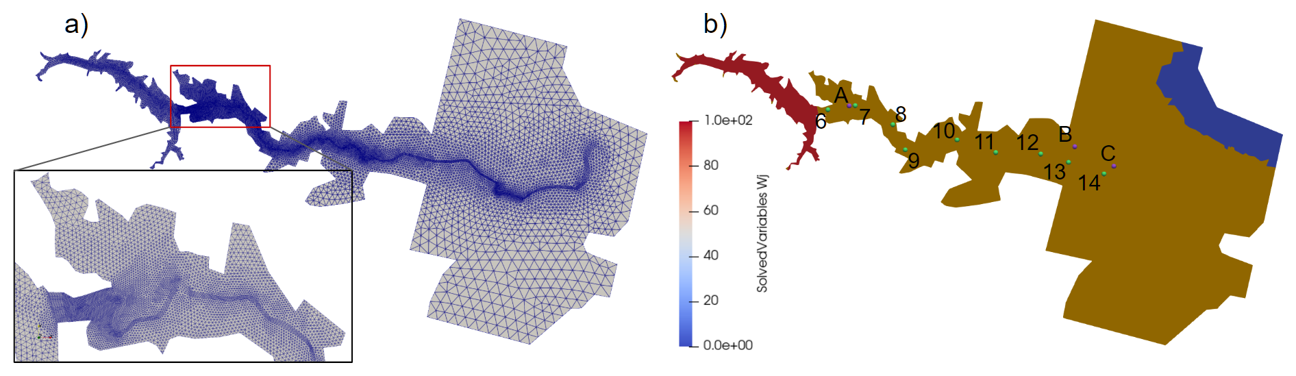
Figure 15 Grid used in the simulation (a) with zoomed view of the upstream refined part, and initial water height (b). Points are the locations of measured data.

Twelve virtual gauge locations are defined along the river valley to monitor the flood wave progression (Fig. 15b). Three gauges (transformers A, B, and C) are used to measure wave arrival times, while nine gauges (P6–P14) record maximum water heights from 1:400 scale laboratory experiments by Electricité de France. The simulated values of arrival times and peak heights are reported in Table 7 alongside the corresponding experimental data and results from TELEMAC’s HLLC solver, widely regarded as the most accurate scheme for this benchmark.

Table 7 Simulation results and relative errors, evaluated against recorded data, for both TELEMAC and SWEpy.

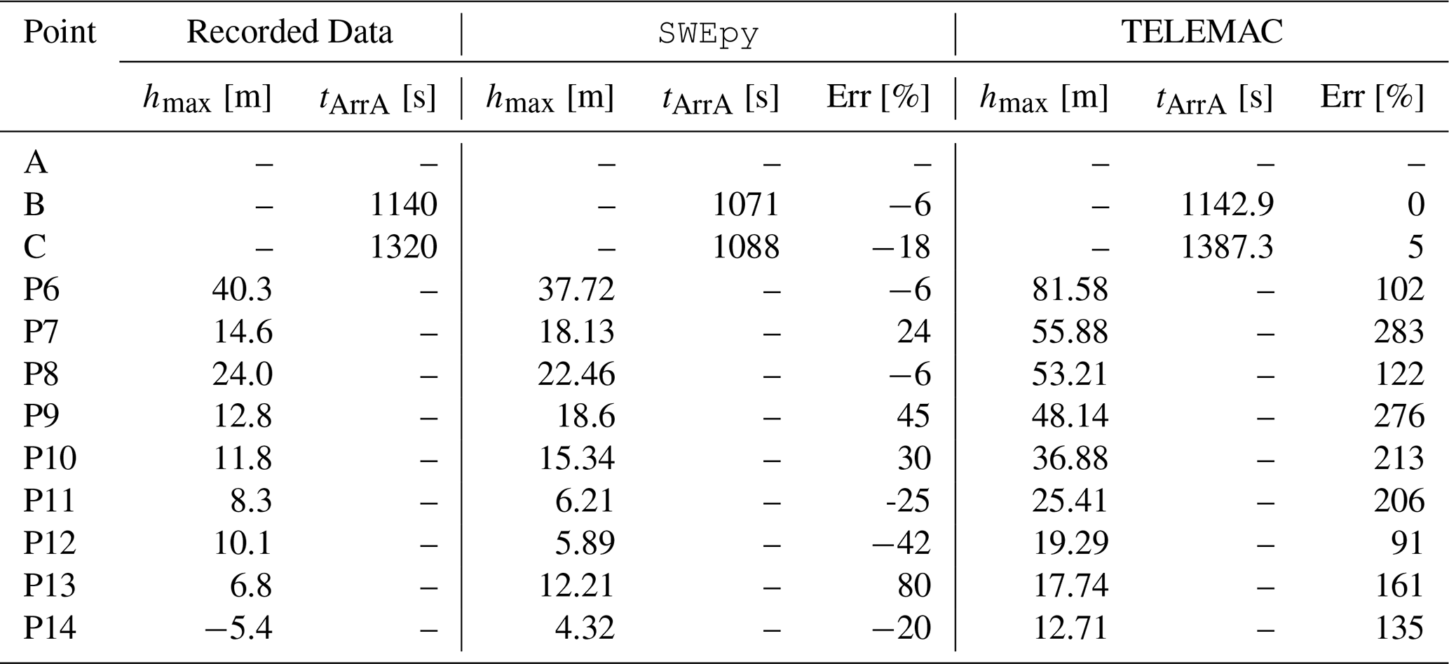
This benchmark provides a rigorous test of SWEpy’s ability to handle complex bathymetry, apply semi-implicit friction for roughness effects, and accurately treat wetting–drying fronts in initially dry cells. While SWEpy exhibits notable discrepancies at certain locations, its relative errors are, in most cases, nearly an order of magnitude smaller than those produced by TELEMAC’s FV solver. As noted in TELEMAC’s validation guide, these discrepancies may stem from several factors: (i) measurement uncertainty in the 1:400 scale physical model, (ii) omission of debris transport and sediment dynamics, and (iii) the fact that the dam breach was not truly instantaneous. In addition, the combination of rapidly varying topography and highly curved flow paths may violate the underlying assumptions of the SWE, further contributing to discrepancies between simulated and observed data.

TELEMAC’s accuracy improves with increasing distance from the dam, suggesting that numerical diffusion is a significant factor in the model and may help explain its closer agreement in arrival-time estimates. Point P13 stands out as a pronounced outlier for both solvers. Its location within a poorly resolved section of the inner riverbank likely contributes to the large discrepancy in the predicted maximum height. To support this hypothesis, nearby points located outside the riverbank record simulated water heights between 4 and 8 m, values that align more closely with the observed data. This poor resolution stems primarily from the coarse bathymetry dataset lifted from the original maps, therefore, finer remeshing would not necessarily resolve this discrepancy.

Given the complex bathymetry and the tightly spaced unstructured grid, some numerical artifacts arose in our first solutions from the interaction between the wet/dry treatment and the impermeable‐wall ghost‐cell boundary conditions. These occur in some border cells where the bathymetry outward normal points away from the domain, i.e., locations where water would naturally exit the computational area. Such cells can act as an artificial source of inflow, as observed in the animations provided in the supplement. In the present case, these artifacts do not significantly affect the solutions presented, since the water height introduced (∼ 0.01 m) is negligible compared to the wave arrival heights (∼ 10 m). However, careful grid construction can help prevent such situations. Figure 16 illustrates the original and corrected bathymetry near domain boundaries, showing a noticeable reduction in spurious water influx after applying the correction.

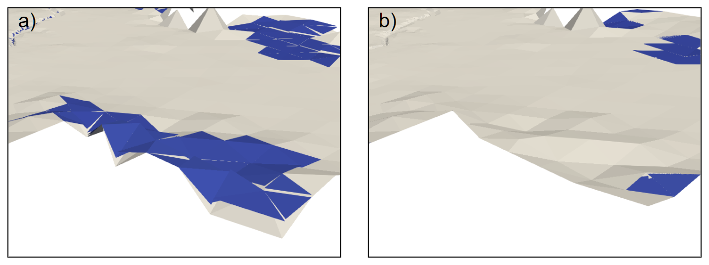
Figure 16 3D View of solution before (a) and after (b) grid correction. Artificial water influx is reduced thanks to the bathymetry fix.

Unfortunately, some artificial inflows remain even after applying this correction procedure. Figure 17 shows the wave arrival at transformers A and C, where the inundation pattern is correctly reproduced but small residual mass contributions from these artifacts are still visible in some cells outside the measurement zones, still with negligible sizes; confirming that these artefacts do not affect the reported results.

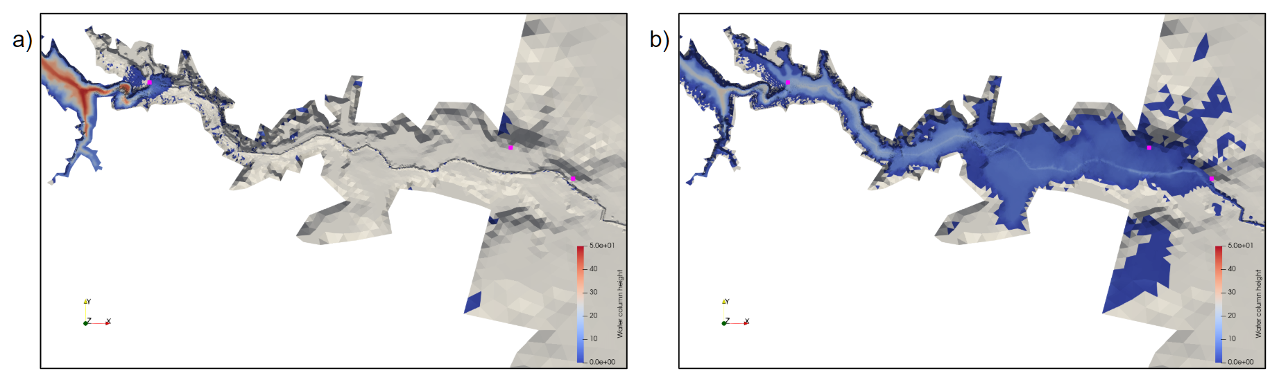
Figure 17 Top-down view of inundation wave arriving at transformer A (a) and C (b). Transformer locations are marked with magenta boxes. Some water influx is present due to errors of the border-wet/dry interaction, but remains outside the measuring zones.

These results confirm that SWEpy can reliably reproduce complex inundation dynamics over irregular terrain while also identifying clear avenues for improvement. Zones with limited topographic resolution would benefit from targeted mesh refinement, and the integration of additional physical processes, such as rheology, sediment transport, and the influence of steep bathymetric gradients or strong flow curvature, could further enhance predictive skill.

5.3 Real-life scenario 2: Maule 2010 tsunami

To evaluate SWEpy's capability for far-field tsunami simulation–specifically its ability to propagate long-period waves over transoceanic distances with minimal numerical dissipation – we reproduce the 2010 Maule tsunami, generated by an M_w 8.8 earthquake along the Chilean subduction zone (Benavente and Cummins, 2013). This event produced measurable signals across the Pacific basin, where Coriolis effects are dynamically relevant and numerical accuracy over very long propagation paths is essential for preserving wave amplitude and shape. This test also enables an assessment of the combined impact of WENO spatial reconstruction and RK4,3 time integration, compared with minmod and explicit Euler methods.

The computational mesh is an equilateral triangular grid generated from GEBCO bathymetry (GEBCO Bathymetric Compilation Group 2024, 2024) via a spherical–Cartesian transformation, containing approximately 10⁶ cells (∼ 536 000 nodes). Because the mesh was constrained to a rectangular bounding box for refinement, additional cells were created at the corners; the effective number of wet cells representing the domain is therefore about 860 000. The initial sea-surface displacement is prescribed from the inversion by Benavente and Cummins (2013) using the Okada fault-slip model, with zero initial velocity. Coriolis effects are included by setting $f={\mathrm{10}}^{-\mathrm{4}}{\mathrm{s}}^{-\mathrm{1}}$, typical in mid-latitude regions (Kundu et al., 2012). Simulations span 24 h of physical time, using adaptive time-stepping with a Courant–Friedrichs–Lewy (CFL) number of 0.25 for explicit Euler integration and 0.5 for RK4,3 integration, applied to each reconstruction–integrator configuration.

Two virtual wave gauges are positioned at the locations of NOAA DART buoys 32 412 (southwest of Lima, Peru) and 21 413 (southeast of Kyoto, Japan), as indicated in Fig. 18. At each gauge, the water-column height is recorded every 60 s of simulated time, yielding continuous time series for the 24 h simulation period. This duration captures the primary tsunami signal and subsequent wave groups at both stations. The numerical results are compared with quality-controlled, rectified DART measurements (Mungov et al., 2005), enabling a direct evaluation of amplitude and phase preservation over basin-scale propagation.

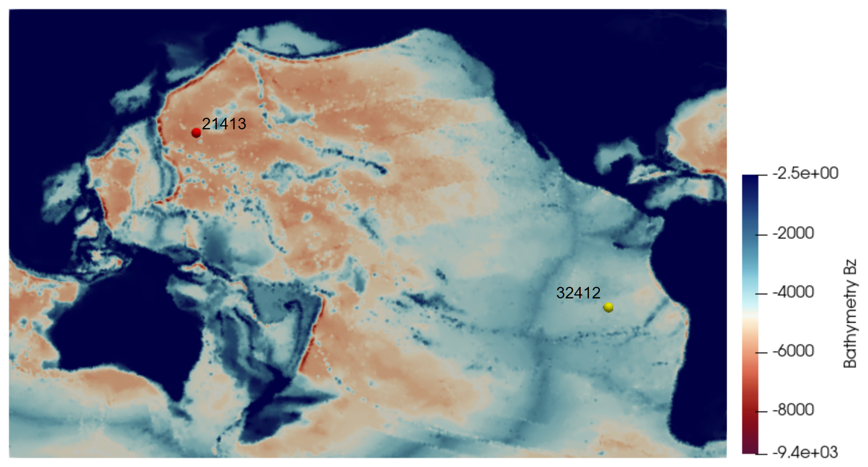
Figure 18 Bathymetry grid employed for the Maule tsunami simulation.

Figure 19 compares the simulated tsunami waveforms at DART buoys 32 412 (panel a) and 21 413 (panel b) with quality-controlled observations and reference simulations from the HySEA model. At buoy 32 412, the WENO reconstruction with explicit Euler integration provides the closest match to the observed primary wave amplitude and timing, and retains secondary oscillations more effectively than the minmod and constant reconstructions. Minmod with a high limiter parameter (ϑ=1.4) reduces phase drift relative to the constant scheme, but still underestimates the amplitude of later wave groups. At buoy 21 413, located in the northwestern Pacific, all SWEpy configurations exhibit greater attenuation of the signal, reflecting the cumulative impact of propagation distance and coarse resolution; here, the WENO scheme again preserves amplitude better than the other reconstructions, with the minmod operator becoming too oscillatory, although the differences are less pronounced. Across both sites, HySEA results at 1.5 million cells show closer agreement with the DART data than SWEpy, consistent with the benefits of higher effective resolution. While WENO incurs a modest computational cost increase over minmod (as explored later), it remains faster than real time for the domain and resolution tested, offering a consistent improvement in waveform fidelity.

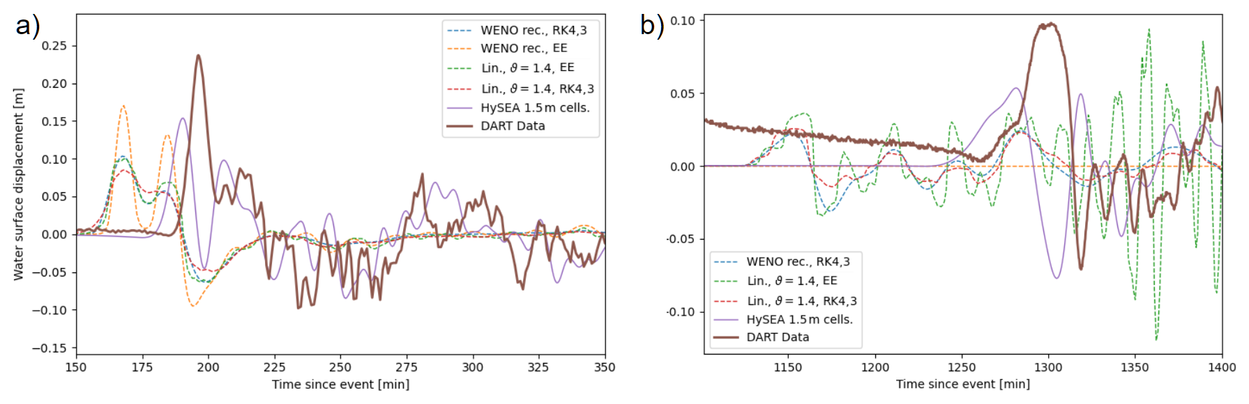
Figure 19 Tsunami profile comparison at DART buoy 32 412 (a) and 21 413 (b). Results from the HySEA model are included for reference. The explicit Euler + WENO result for buoy 21 413 is omitted because of high-frequency oscillations that obscured the primary tsunami signal.

The explicit Euler + WENO result is not shown for buoy 21 413 because the combination of explicit Euler and coarse resolution over the long propagation path generated high-frequency oscillations that obscured the primary tsunami signal (Fig. 20). Table 8 quantifies the performance of each configuration by comparing the maximum wave height H_max and arrival time T_arr of the first wave against the DART observations. These metrics complement the full time-series comparison by highlighting differences in amplitude attenuation and phase shift.

Table 8 Performance summary of SWEpy configurations and HySEA for the Maule 2010 tsunami benchmark. Maximum surface displacement H_max [m] and arrival time T_arr [min] are extracted at the first wave crest for DART buoys 32 412 (Lima) and 21 413 (Kyoto). Relative errors (%) are computed with respect to the DART observations.

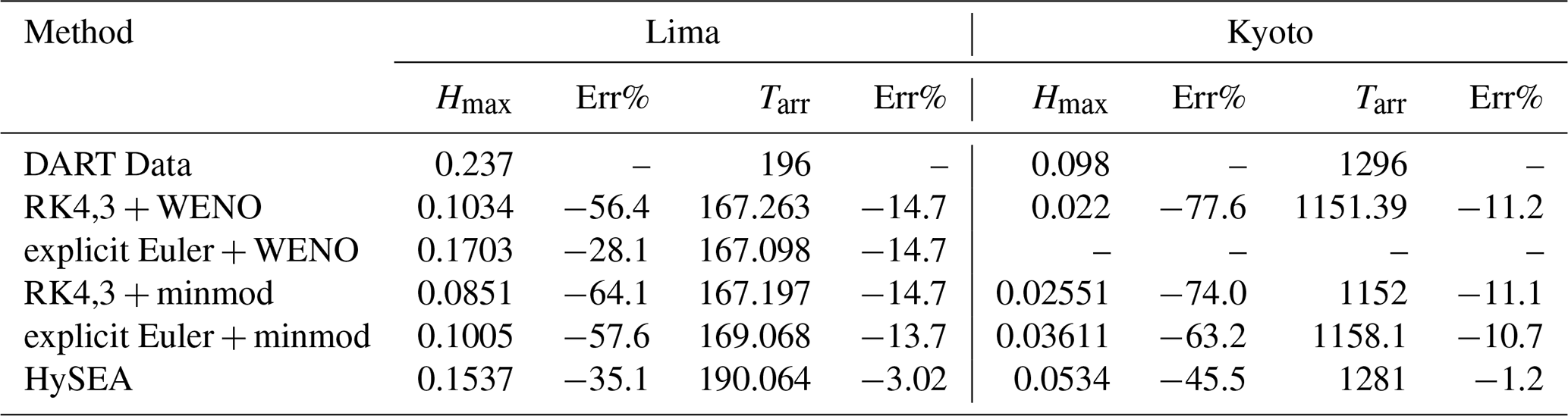
These metrics indicate that SWEpy underestimates the maximum crest height and predicts earlier arrivals at both stations, whereas HySEA exhibits smaller amplitude bias – particularly at Lima – and reduced phase error, consistent with the visual comparisons in Fig. 19. The differences likely reflect a combination of: (i) source smoothing introduced during interpolation to the computational grid, (ii) bathymetric resolution, with the HySEA configuration employing nearly twice as many cells, and (iii) projection-related errors from the spherical–Cartesian transformation, given that HySEA solves the SWEs directly on the sphere. This last point is important, since we only converted the grid to Cartesian coordinates via a haversine transformation; however, formulas for fluxes, cell side length, and cell area were maintained, when they should be calculated considering transformations. Quantifying the contribution of each factor is left for future work, with the aim of guiding targeted improvements to SWEpy's far-field performance through a rigorous treatment of the spherical case.

While initially producing the most accurate waveforms at the near-field gauge, the explicit Euler time integrator in combination with the WENO reconstruction develops spurious high-frequency oscillations after extended transoceanic propagation. These oscillations overwhelm the primary tsunami signal at the Kyoto gauge, making the solution unsuitable for quantitative analysis. Figure 20 illustrates the modeled free-surface elevation at the moments when the wave passes the Lima and Kyoto DART buoys, for both explicit Euler + WENO and RK4,3 + WENO configurations, highlighting the marked difference in solution smoothness.

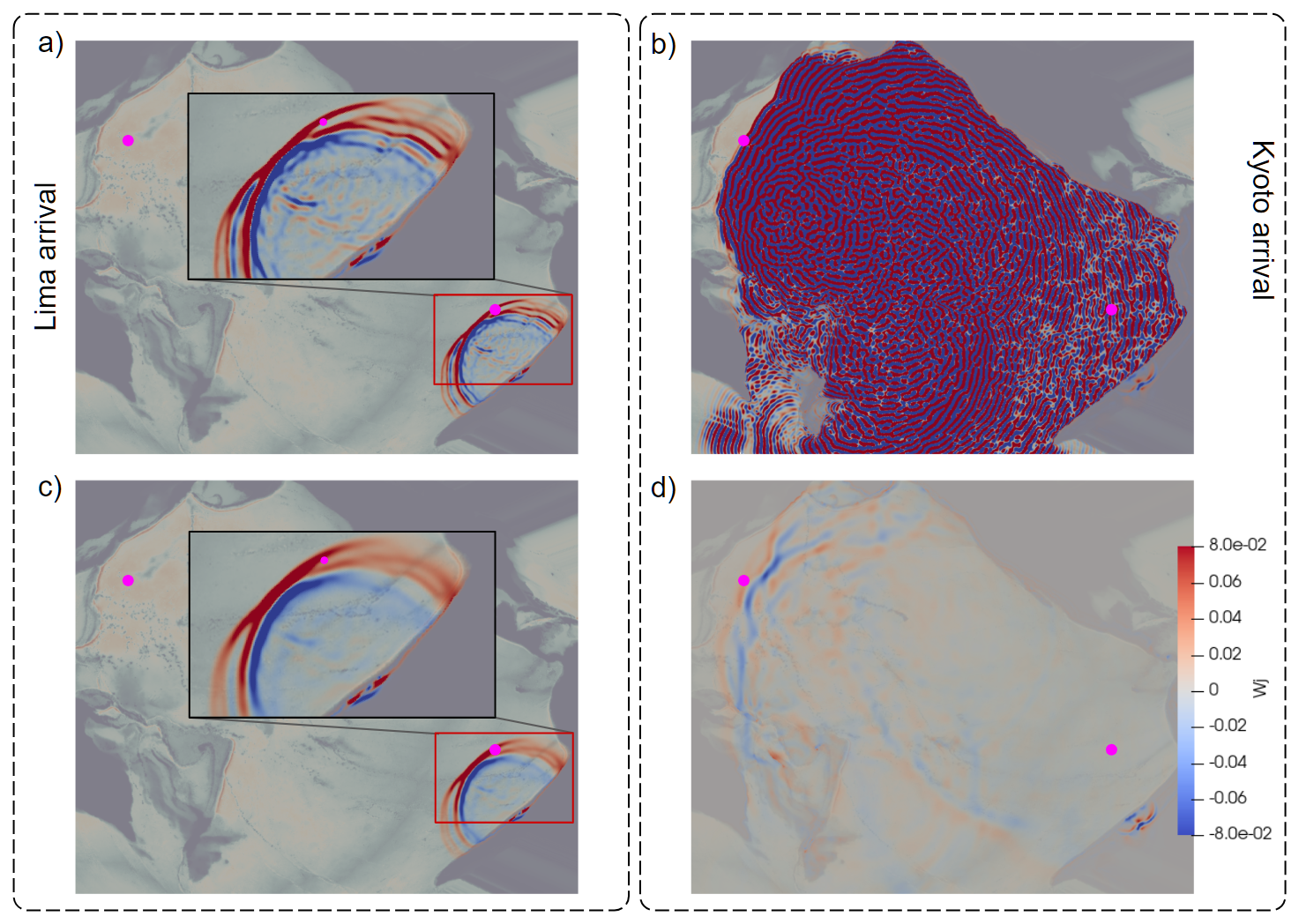
Figure 20 Snapshots of simulated free-surface elevation for the Maule 2010 tsunami at the times when the leading crest passes the locations of DART buoys 32 412 (Lima) and 21 413 (Kyoto). Insets show zoomed view of wave at Lima buoy. Panels (a) and (b) correspond to explicit Euler integration, and panels (c) and (d) to RK4,3 integration. Buoy locations are marked with magenta circles. These views provide basin-scale context for the time-series comparisons in Fig. 19.

Control of these oscillations could, in principle, be achieved by reducing the CFL number; however, this would further increase numerical diffusion. Even with a reduced value of CFL =0.2, the oscillations remain excessive by the time the wave reaches Kyoto, producing spurious amplitudes of approximately 0.3 m, while simultaneously reducing the maximum height at Lima to 0.14 m.

Spurious oscillations in Fig. 20b may develop as a result of the interaction between the high-order reconstruction and the temporal discretization, due to the reduced level of numerical diffusivity and, consequently, the lack of an effective numerical dissipation mechanism to control the generated oscillations. In addition, the spatial mesh and, in particular, the way boundary conditions are imposed may also contribute to this behavior (see inset of Fig. 20a).

This phenomenon was investigated through an auxiliary numerical experiment in which a soliton propagating along a channel with periodic boundary conditions was considered; see Sect. S7.2 Instability study: impact of temporal discretization in the User Manual & Technical Reference (Meza et al., 2026). The results show that simulations employing a more diffusive reconstruction do not generate spurious oscillations, whereas the explicit Euler + WENO combination leads to the development of resonance-type oscillations. These oscillations may partially explain the spurious oscillatory patterns observed in the figure, ultimately giving rise to numerical convective instabilities in space.

To explore grid convergence, additional runs were performed with closer HySEA-SWEpy resolution agreement, using results from a HySEA run with a ∼ 250 000 element resolution as reference, and a SWEpy grid of ∼ 280 000 (effective) elements. Also, to assess the reduction of oscillatory behaviour in the explicit Euler + WENO case, a run with a CFL number of 0.15 was performed. Figure 21 shows the output at the DART buoys locations.

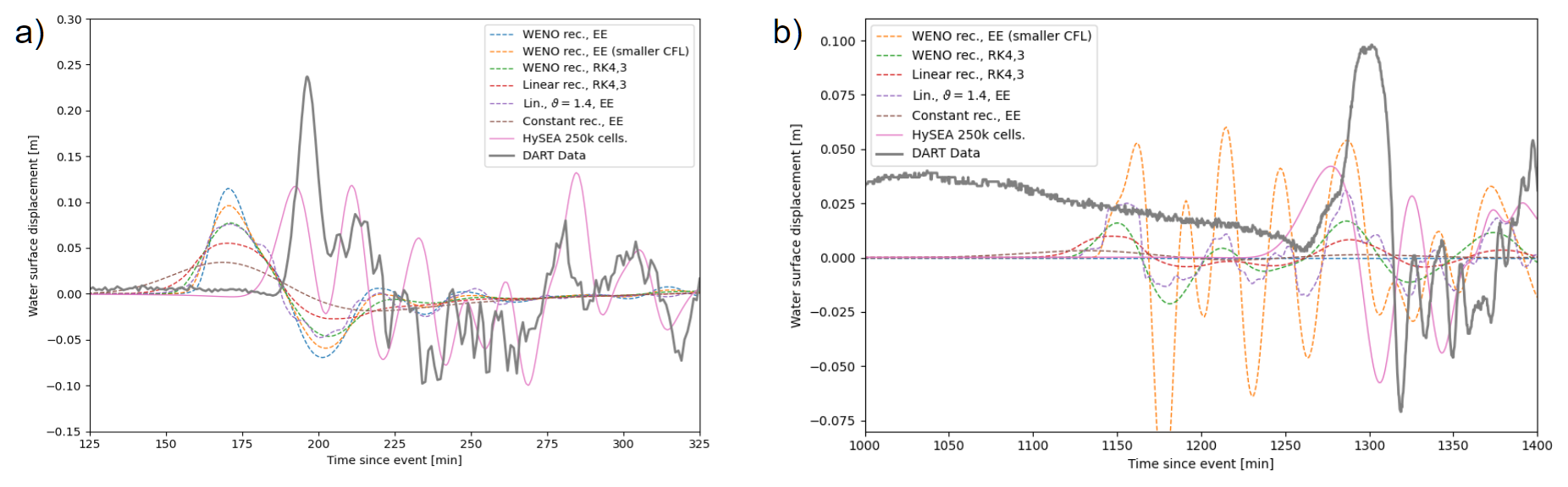
Figure 21 Tsunami profile comparison at DART buoy 32 412 (a) and 21 413 (b) for the coarser grids. Once again, results for the explicit Euler + WENO at the Kyoto buoy have been omitted.

These results confirm two points discussed above: (1) The resolution of the mesh is indeed correlated to the arriving wave amplitude, with both SWEpy and HySEA achieving similar accuracy; and (2) control of the spurious oscillations via the CFL number is achievable with the trade-off of some quality degradation. This confirms that, with similar spatial resolution, SWEpy can attain comparable initial wave amplitudes to HySEA.

To illustrate computational efficiency and the benefits of GPU acceleration on a real-life problem, the Maule 2010 scenario was repeated on a different simplified, non linearized, mesh of approximately 2.5×10⁵ elements, using different combinations of time integrators and spatial reconstructors. To test GPU-parallelization speedups, a serial, single core, CPU-only version of SWEpy was used as reference, where CuPy was replaced by the traditional NumPy. At this reduced resolution, wave-height errors ranged from −98 % to −13.4 % and arrival-time errors from −2 % to 26.5 % relative to DART observations, reflecting the expected degradation in solution quality. Despite this, execution times for all configurations were faster than real time (Table 9).

Table 9 Comparison of methods explicit Euler + minmod (fastest) and RK4,3 + WENO (slowest). CPU times correspond to simulations ran on a serial CPU-only implementation. GPU times correspond to the present CuPy implementation.

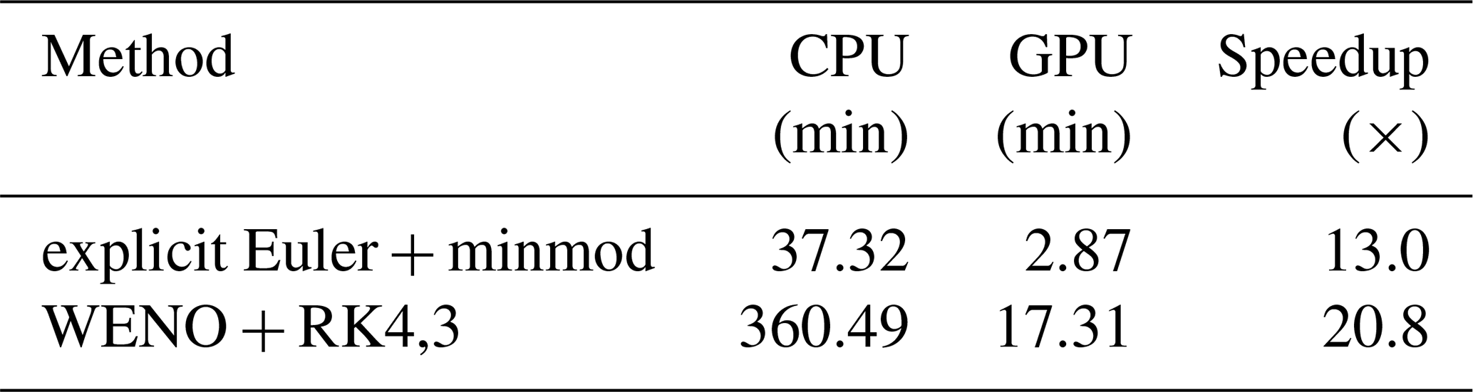
Tests were performed on an Intel^® Core^TM i5-10300H CPU (10th generation) and an NVIDIA GeForce GTX 1650 GPU, both consumer-grade components released more than six years prior to writing. However, this performance comparison is intended to illustrate the benefits of GPU acceleration within the SWEpy framework using a standard single-core CPU baseline, rather than providing a hardware-optimized or scalability-focused performance study across architectures. These results underscore SWEpy’s ability to deliver high-performance simulations on widely available, non-specialized hardware.

As a whole, the Maule 2010 benchmark results demonstrate SWEpy’s ability to reproduce the main features of basin‐scale tsunami propagation, including crest arrival timing, amplitude decay, and the modulation of subsequent wave groups. Among the tested schemes, the WENO reconstruction consistently yields the most accurate far‐field waveforms, though in combination with explicit Euler integration it can develop basin‐scale oscillations that obscure the signal at distant stations (Fig. 20). These oscillations persist even under reduced CFL numbers, with the trade‐off of increased diffusion and degraded amplitudes at nearer gauges. The RK4,3 integrator mitigates this instability while preserving much of WENO’s accuracy, making it the most balanced choice for long‐range simulations. GPU acceleration enables faster‐than‐real‐time performance even for the most demanding configuration, with speedups exceeding 20× on consumer‐grade hardware with respect to the serial implementation. Together, these results confirm the model’s applicability to large‐domain tsunami scenarios, while highlighting clear paths for improvement in projection accuracy, bathymetric resolution, and source initialization to close the remaining gaps with higher‐resolution reference models such as HySEA.

6 Conclusions

We presented SWEpy, an open-source GPU-accelerated (CUDA) Python package for the SWEs on unstructured triangular grids. The solver addresses hydrodynamic hazard scenarios across a wide range of spatial and temporal scales, from localized flooding to transoceanic tsunami propagation, by combining conservative numerical schemes with high-performance computing capabilities on consumer-grade hardware. SWEpy's modular design enables researchers to adapt or extend the code for specific applications while maintaining computational efficiency and numerical stability. Core features include robust wetting/drying treatment, low-diffusion reconstructions, and well-balanced source-term discretizations, which allow for reliable simulations in complex, high-risk environments.

To evaluate spatial accuracy, a grid-refinement study was conducted against a numerically converged reference solution computed with SWEpy on the finest mesh. The results demonstrated a monotonic reduction in L² error with decreasing Δx. Constant reconstruction achieved better-than-first-order accuracy, while both linear and quadratic variants exhibited second-order convergence. Although the quadratic WENO reconstruction did not reach full third-order accuracy due to flux–bathymetry coupling, it reduced errors by an average of ∼ 58 % relative to the linear reconstruction at matched resolution. Importantly, across all refinements, the well-balanced source-term discretization preserved steady-state conditions, providing a reliable numerical baseline for subsequent real-case validations.

Building on this, the accuracy and robustness of SWEpy, particularly its wet/dry treatment, were further assessed using the well-known Conical Island laboratory experiment, a benchmark widely used in coastal hydrodynamics. This configuration provides high-quality measurements of wave transformation, run-up, and diffraction around an isolated obstacle. SWEpy successfully reproduced the main free-surface patterns and wetting–drying transitions with a good agreement to experimental observations, confirming its ability to capture the fundamental physics of wave–structure interaction. Beyond serving as a verification benchmark, this experiment establishes confidence in the solver’s applicability to more complex and operationally relevant scenarios, including large-scale dam-break inundations and basin-scale tsunami propagation over realistic bathymetry.

Real-case applications such as the Malpasset dam-break and the Maule 2010 tsunami highlight different aspects of the solver's performance. In the Malpasset case, characterized by a short-duration, high-gradient flood in a confined valley, SWEpy maintained physically realistic wetting–drying behavior, conserved mass across advancing fronts, and achieved substantially lower water level errors than TELEMAC’s FV solver, with arrival times generally within ∼ 18 % of observations. In contrast, the Maule tsunami case exposed current limitations in large-scale basin-propagation. All SWEpy configurations underestimated the first-wave amplitude and predicted earlier arrival times at both DART buoys. Among the tested schemes, WENO + EE performed best, with −28 % error in amplitude and −15 % error in arrival time, although it developed high-frequency oscillations over long propagation distances. The WENO + RK4,3 scheme remained oscillation-free and reduced dissipation and phase drift relative to lower-order schemes; however, notable amplitude and timing biases persisted. These discrepancies likely stem from source smoothing during interpolation, projection errors between spherical and Cartesian coordinates (in contrast to HySEA’s spherical formulation), and coarser bathymetric resolution. Together, these findings identify clear directions for improvement, including enhanced projection accuracy, improved source initialization, and refined mesh resolution, which are critical for achieving stronger far-field predictive capability at ocean-basin scales.

From a computational perspective, SWEpy delivers high-performance even on modest hardware that is more than six years old at the time of writing. A performance and scalability study highlighted both the advantages of GPU acceleration and its limitations, particularly regarding kernel launch overhead. GPU and VRAM throughput were analyzed to identify which configurations most effectively utilize the hardware. Using a simplified unstructured mesh of approximately 2.5×10⁵ elements, the 24 h Maule 2010 tsunami scenario (in its most demanding reconstruction and timestep configuration) was simulated in approximately 17 min on an NVIDIA GeForce GTX 1650 laptop GPU. This corresponds to a speedup of approximately ∼ 2100 % relative to the single-core CPU baseline, executed on an Intel^® Core^TM i5-10300H processor. These results, enabled by extensive CuPy-based vectorization and memory-efficient data structures, demonstrate that large-scale SWEs simulations on unstructured grids can be performed well within real time on widely accessible systems, significantly lowering the barrier to high-performance hydrodynamic modeling while maintaining scalability for more detailed studies.

SWEpy is built on the CuPy library, which is primarily developed for the NVIDIA CUDA ecosystem. While CuPy offers experimental support for AMD GPUs through the HIP/ROCm interface, all validation and performance results presented here rely exclusively on the stable CUDA backend to ensure numerical reproducibility, performance consistency, and software robustness in this initial release. As CuPy’s multi-backend capabilities continue to mature, SWEpy is well positioned to benefit from broader GPU compatibility without requiring fundamental changes to its core implementation.

Despite these advances, several limitations remain, as revealed by the validation studies. In the Maule 2010 tsunami case, amplitude underestimation and arrival-time biases indicate the need for improved bathymetric interpolation, reduced projection error between spherical and Cartesian coordinates, and higher-resolution meshes for basin-scale applications. In the Malpasset case, complex gridding and bathymetry interactions suggest that the wet/dry treatment may interact with ghost-cell boundary conditions, potentially introducing artificial sources of mass influx, which warrants further investigation. Additionally, the sub-third-order convergence observed for the quadratic WENO scheme indicates that flux–bathymetry coupling remains a limiting factor for spatial accuracy. More broadly, the solver inherits the hydrostatic assumption of the SWEs, which may introduce inaccuracies in steep or highly curved flows where vertical accelerations are significant. Ongoing development efforts are therefore focused on improving bathymetric handling, coordinate projection, spatial accuracy, and physical modeling to enhance the robustness and applicability of SWEpy.

From a software development perspective, the roadmap for SWEpy emphasizes continued optimization of GPU efficiency and further refinement of its modular architecture. This design facilitates community contributions and allows individual components – such as source terms, numerical schemes, and physical models – to evolve independently. While the current implementation targets single-GPU execution, future work may explore improved utilization of multi-core CPUs through process-based parallelism using Python’s native multiprocessing or CuPy-native kernel customization and fusion features. In contrast, implementing efficient MPI-based parallelization for unstructured grids entirely in Python remains challenging, as communication overhead can outweigh computational gains. Without hybrid C$++$/Python approaches – such as MPI wrappers around compiled kernels – pure Python MPI solutions often diminish the benefits of parallel execution. These considerations reinforce the current emphasis on GPU-centric acceleration, where high throughput can be achieved within a unified and accessible Python framework.

We anticipate that the flexibility of SWEpy provides a strong foundation for extending its capabilities beyond the current scope. Planned developments include additional source-term modules for rainfall and infiltration to support catchment-scale hydrology, as well as rheological models for non-Newtonian fluids to simulate landslides, tailings dam breaches, snow avalanches, and debris flows. The framework is also well suited for incorporating two-layer shallow water formulations (2LSWE), following recent advances in CU-type schemes (Cao et al., 2024; Liu, 2021a), to model stratified and two-phase flows such as water–mud avalanches or estuarine mixing. These enhancements, together with ongoing improvements in bathymetric representation, mesh refinement, and large-scale projection accuracy, will further strengthen the solver’s predictive capabilities across a broad spectrum of hydrodynamic hazards. By maintaining its modular, open-source, and GPU-accelerated design, SWEpy is well positioned to evolve into a versatile and high-performance modeling framework that bridges the gap between research prototypes and operational tools for flood and tsunami risk assessment worldwide.

Appendix A: Reconstruction Operators

A1 Linear (Minmod) Reconstruction

The minmod linear reconstruction is detailed in Algorithm A1.

Algorithm A1 Minmod linear reconstruction.

1:

identify neighbors of each cell (cf. group Ω_jk in Fig. 3)

2:

construct planes passing through the mean value of the variable at the barycenters of the cell and its neighbors.

3:

calculate ((q_x)_j,(q_y)_j)

4:

select the plane whose gradient's magnitude is lowest among its three constructed planes

5:

for each cell do

6:

for each side do

7:

if not mean value at cell<reconstructed value at midpoint<mean value at side's neighbor then

8:

impose a constant plane passing through mean value of the variable over the cell

9:

end if

10:

end for

11:

end for

This ensures monotonicity by selecting the least oscillatory interpolant. The algorithm is implemented in parallel for all cells in the SWEpy code by operating arrays containing the mentioned quantities.

A2 Quadratic WENO Reconstruction

The quadratic WENO reconstruction is summarized in Algorithm A2, which outlines the steps for computing the operator on unstructured triangular grids.

Algorithm A2 Quadratic WENO reconstruction.

1:

identify neighbors of each cell (cf. group Ω_jk in Fig. 3)

2:

identify neighbors of neighbors of each cell (cf. group Ω_jkl in Fig. 3)

3:

for each cell do

4:

Construct quadratic polynomial interpolator u_q (cf. Eq. A1)

5:

Construct linear interpolators $p_{\mathrm{1},j},p_{\mathrm{2},j},p_{\mathrm{3},j},p_{\mathrm{4},j}$

6:

Set linear weights ${\mathit{\gamma }}_{\mathrm{0}},{\mathit{\gamma }}_{\mathrm{1}},{\mathit{\gamma }}_{\mathrm{2}},{\mathit{\gamma }}_{\mathrm{3}},{\mathit{\gamma }}_{\mathrm{4}}$

7:

Calculate smoothness indicators ${\mathit{\beta }}_{\mathrm{0}},{\mathit{\beta }}_{\mathrm{1}},{\mathit{\beta }}_{\mathrm{2}},{\mathit{\beta }}_{\mathrm{3}},{\mathit{\beta }}_{\mathrm{4}}$ (Eq. 2.8 in Zhu and Qiu, 2018)

8:

Calculate corrector τ for WENO-Z procedure (Eq. 2.13 in Zhu and Qiu, 2018)

9:

Calculate and normalize nonlinear weights $w_{\mathrm{0}},w_{\mathrm{1}},w_{\mathrm{2}},w_{\mathrm{3}},w_{\mathrm{4}}$

10:

Construct reconstruction operator over cell as ${\stackrel{\mathrm{̃}}{q}}_j=\frac{w_{\mathrm{0}}}{{\mathit{\gamma }}_{\mathrm{0}}}\left(p_{\mathrm{0}}-{\sum }_{k=\mathrm{1}}^{\mathrm{4}}{\mathit{\gamma }}_k{p}_{k,j}\right)+{\sum }_{k=\mathrm{1}}^{\mathrm{4}}{w}_k{p}_{k,j}$

11:

end for

The detailed calculation procedure for the quadratic polynomial $p_{j_{\mathrm{0}}}(x,y)$ relies solely on geometric information associated with the control cell Ω_j. Consider the quadratic form:

$$\begin{array}{}\text{(A1)}& p_{j_{\mathrm{0}}}(x,y)=a_{\mathrm{0}}+a_{\mathrm{1}}x+a_{\mathrm{2}}y+a_{\mathrm{3}}{x}^{\mathrm{2}}+a_{\mathrm{4}}{y}^{\mathrm{2}}+a_{\mathrm{5}}xy,\end{array}$$

shown in Eq. (27), the associated integrals in the construction of the quadratic polynomials and smoothness indicators are calculated exactly.

This polynomial approximates the mean values over the stencil cells and exactly reproduces the mean in ${\mathrm{\Omega }}_{j_{\mathrm{0}}}$. The associated integrals for smoothness indicators are computed exactly. Since the system is overdetermined (9 equations for 5 coefficients), it is solved via least-squares: given Ma=Δq,

$$\begin{array}{}\text{(A2)}& \mathit{a}\stackrel{\mathrm{lsq}}{=}(M^{t}M{)}^{-\mathrm{1}}{M}^t\mathrm{\Delta }\mathit{q}.\end{array}$$

This approach ensures high-order accuracy while preserving well-balancing in the CU scheme. A further detailed explanation of the reconstructor and its usage in the CU scheme will be in Fuenzalida Alarcón et al. (2025).

A3 Wet/dry treatment

The positivity-preserving correction for wet/dry fronts is outlined in Algorithm A3.

Algorithm A3 Positivity preserving wet/dry reconstruction.

1:

find cells at the wet/dry front

2:

for each cell in front do

3:

determines if the cell has one or two dry vertices

4:

if cell has two dry vertices then

5:

$v_{\mathrm{1}}:=(x_{jk\mathrm{1}},y_{jk\mathrm{1}})\leftarrow \mathtt{\text{dry vertex 1}}$

6:

$v_{\mathrm{2}}:=(x_{jk\mathrm{2}},y_{jk\mathrm{1}})\leftarrow \mathtt{\text{dry vertex 2}}$

7:

$v_{\mathrm{3}}:=(x_j,y_j)\leftarrow \mathtt{\text{cell barycenter}}$

8:

$B_{jk\mathrm{1}},B_{jk\mathrm{2}},W\leftarrow \mathtt{\text{bathymetry at }}{v}_{\mathrm{1}}\mathtt{\text{, bat. at }}{v}_{\mathrm{2}}\mathtt{\text{, cell mean water level}}$

9:

replace reconstruction with plane passing through (v₁,B_jk1), (v₂,B_jk2), and (v₃,W)

10:

else if cell has one dry vertex then

11:

$v_{\mathrm{1}}:=(x_{jk\mathrm{1}},y_{jk\mathrm{1}})\leftarrow \mathtt{\text{dry vertex}}$

12:

$v_{\mathrm{2}}:=(x_{jk\mathrm{2}},y_{jk\mathrm{2}})\leftarrow \mathtt{\text{wet vertex}}$

13:

$v_{\mathrm{3}}:=(x_j,y_j)\leftarrow \mathtt{\text{cell barycenter}}$

14:

$B_{jk\mathrm{1}},w,W\leftarrow \mathtt{\text{bat. at }}{v}_{\mathrm{1}}\mathtt{\text{, cell mean w.l., }}\mathrm{3}\mathrm{/}\mathrm{2}\text{(w - cell mean bat.)+bat. at }{v}_{\mathrm{2}}$

15:

replace reconstruction with plane passing through (v₁,B_jk1), (v₂,W), and (v₃,w)

16:

end if

17:

end for

This algorithm corrects reconstructions yielding negative depths by fitting a mass-conserving linear plane, executed in parallel on the GPU for efficiency.