psit 1.0: a system to compress Lagrangian flows

Meteorological simulations produce large amounts of data, which can represent a challenge when trying to store, share, and analyze it. As weather and climate models increasingly simulate the atmosphere at higher spatio-temporal resolution, it becomes imperative to compress the data effectively. While compression algorithms exist for weather data stored in a gridded Eulerian frame, there are, to date, no specialized alternatives for data stored in the Lagrangian frame. In this study, we present psit, a system to compress weather data stored in the Lagrangian frame. The system works by mapping the trajectories to a grid structure, performing additional encodings on these, and passing them to either the JPEG 2000 image compression algorithm or SZ3. The specialty of the algorithm is the mapping phase and the following encodings, which generate the grids in a way that allows the aforementioned compression algorithms to perform well. To gauge the performance of psit, we test a variety of metrics. We demonstrate that in the majority of cases, equivalent or superior compression performance is attained through the utilization of psit as opposed to naive compression with ZFP or SZ3. We also compare compression with measurement inaccuracies. Here, we show that the density of 168 hour long trajectories compressed with a ratio in the range of 30 to 40 behaves similarly to trajectories calculated from uncompressed wind fields with additional random perturbations with magnitude of 0.1 m s⁻¹ in the horizontal and around $\mathrm{6}\times {\mathrm{10}}^{-\mathrm{3}}$ Pa s⁻¹ in the vertical component. Additionally, we conduct two case studies in which we discuss the impact of compression on the study of warm conveyor belts associated with extratropical cyclones and the impact of compression on the radioactive plume prediction of the Fukushima incident in 2011.

1 Introduction

With advancements in parallel computing and the introduction of larger and more powerful HPC systems, the size and complexity of today's meteorological models have increased significantly. Such an increase in complexity leads to a rise in the amount of output data, reaching the range of dozens of petabytes (Hoefler et al., 2024, 2023). Storing and analysing such a massive amount of data poses significant challenges. Consequently, different approaches have been developed to address this issue. One approach works by reducing the number of elements that are stored (Tintó Prims et al., 2024). In the case of weather data, this can be achieved, for example, by reducing the grid resolution of the stored data or decreasing the temporal interval at which data is stored. This approach is already in use for the ERA5 weather dataset (Tintó Prims et al., 2024). A second approach that is commonly used focuses not on reducing the number of elements but on decreasing the space occupied by each of them. This is the field of compression algorithms, which reduce data size by exploiting structure present in the underlying data, a technique commonly used in multimedia, as seen in formats like JPEG (Wallace, 1991) and H.265 (Sullivan et al., 2012). For the compression of scientific data, we usually prefer lossy compression, as, due to the inherent noise present, lossless compression algorithms will not be able to achieve large compression ratios (in the range of 2 to 4 times). We will therefore focus on lossy compression techniques.

Several lossy compression algorithms for the compression of multidimensional floating-point data have been developed. A (non exhaustive) list includes: SZ3 (Liang et al., 2023b, 2018; Zhao et al., 2021), ZFP (Lindstrom, 2014; Diffenderfer et al., 2019), and THRESH (Ballester-Ripoll et al., 2019; Ballester-Ripoll and Pajarola, 2015). Previous research by Tintó Prims et al. (2024) has demonstrated the effectiveness of these floating-point compression algorithms in compressing weather data in the Eulerian frame. There are also specialized compression algorithms developed specifically for weather data, such as VAEformer (Han et al., 2024), an autoencoder- based compression algorithm designed for the compression of the ERA5 weather dataset. Hence, a wide variety of compression algorithms exist that can be utilized for the compression of weather data in the Eulerian frame.

On the other hand, meteorologists not only work with the Eulerian representation but also often consider a Lagrangian one. In this representation, we do not have a multidimensional grid but instead track the position and properties, like temperature, of small air parcels carried by the wind, resulting in so called trajectories. This representation is crucial for certain types of analysis, such as identifying warm conveyor belts (Wernli and Davies, 1997b; Joos and Wernli, 2012; Schemm et al., 2013) or stratosphere-troposphere exchanges (Holton et al., 1995; Škerlak et al., 2014). However, here we also face the problem of an increase in output data and therefore seek to compress it. Compared to multidimensional grid data, the landscape of compression algorithms for weather data trajectories is much poorer. There are mainly two fields related to this, first is the compression of trajectory data, where research mostly focuses on data generated from GPS tracking of vessels or, more generally, the movement of objects in space over many time steps (Makris et al., 2021). Examples of such algorithms include Dead-Reckoning, Douglas-Peuker, and Time-Ratio (Makris et al., 2021), all of which reduce data volume by strategically removing individual time steps while preserving the general trajectories. However, these methods are not suitable for compressing trajectories originating from weather data for two main reasons. First, the number of time steps in weather trajectories is typically much lower than in GPS trajectories. For GPS trajectories, the number of time steps might be in the 10 000 range, while for weather trajectories, depending on the use case, one might work with only a few dozen (e.g., hourly to six hourly temporal resolution). Additionally, removing time steps from weather trajectory data may not be permissible due to the specific requirements of subsequent research. Secondly, weather trajectory data often includes additional variables, such as temperature or potential vorticity, that are of interest along the trajectories. The above mentioned trajectory compression algorithms do not account for these additional variables, only for the position, which makes them unsuitable for compressing such weather data. The second research field related to this is the compression of unstructured mesh data. Different methods like (Liang et al., 2023a; Ren et al., 2024; Wu et al., 2025) exists and a recent survey has been made by Di et al. (2025). But quite a lot of them are not directly designed for time series data, but focus on other aspects such as point clouds (Quach et al., 2022) or medical data (Al-Salamee and Al-Shammary, 2021). The research that focuses on time series data (Chiarot and Silvestri, 2023) mostly is in the field of internet of things and not on weather data. So we can see that there appears to be a gap when it comes to the compression of trajectories originating from weather data.

To address this gap, we present psit, a lossy compression method for Lagrangian flow data. Psit works by transforming the trajectory data into 2D grids and passing those grids to existing compression algorithms, specifically JPEG 2000 (Skodras et al., 2001) and SZ3, where JPEG 2000 has shown its potential in internal research and is used by the visualization community due to its adaptive scalability property (Woodring et al., 2011). This approach leverages the refined performance of these compression algorithms to create a compression pipeline specifically designed for trajectory weather data.

2 Method

The general idea behind psit is to take the trajectories and intelligently transform them so that they can be passed to existing compression algorithms. This general pipeline is illustrated in Fig. 1. The input expected by the dense data compressors (JPEG 2000 and SZ3) consists of 2D arrays (i.e., grids), which ideally should be smooth, i.e., the difference between neighboring entries of the array should be small. Note that a single 2D array (representing one channel) can be passed to the JPEG 2000 algorithm, as it is able to handle an arbitrary number of channels (individual 2D arrays) and is not limited to the default three color channels (red, green, and blue) used for images. Therefore, in the first step (the mapping phase), the trajectories are transformed into such grids. During this mapping, it is crucial to assure the resulting grids smoothness, as greater smoothness allows both compression algorithms to perform more effectively. Once the mapping step is completed, encoding schemes can be applied to them, namely delta and color encoding. These encoding schemes modify the grids in a way that leads to better compression performance for the previously mentioned compression algorithms. In the next step, the encoded grids are passed to a dense data compressors to perform the compression, and the compressed data is subsequently stored to disk. These four steps form the basis of psit and are discussed in more detail in the rest of this section.

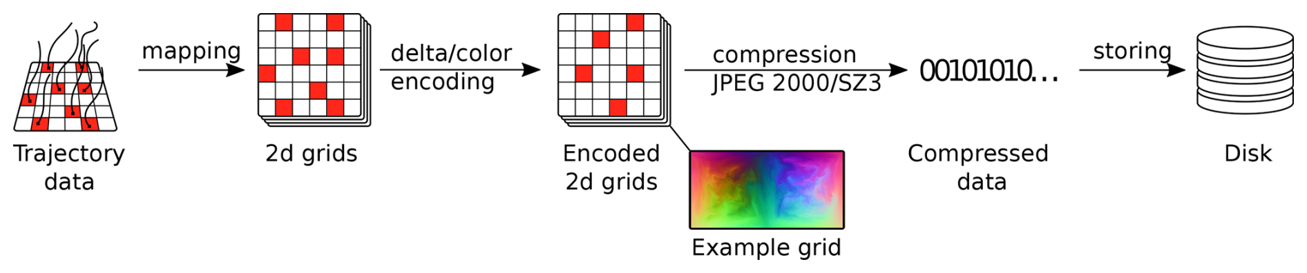
Figure 1 The compression pipeline of psit. In the first step, the mapping phase, trajectory data is converted into grid data. After these grids have been created they can be manipulated in order to have better compression performance, namely delta and color encoding. Then as a final step the grids are compressed with either JPEG 2000 or SZ3 and stored to disk. The decompression works the same, but in the opposite direction.

The decompression phase mirrors the compression process: the data is loaded from disk and then decompressed using the same algorithm employed during compression (e.g., JPEG 2000). After this, the encoded grids are decoded (delta and color decoding) to obtain the mapped 2D grids. Finally, these 2D grids are transformed back into trajectories using an inverse mapping of the original one. After this step, the decompression is complete, and the trajectory data should closely match the original data, with only the errors introduced by the compression algorithm differentiating them.

2.1 Input data

In the following, we will provide a definition of what a trajectory and a possible input file are in order to establish a common basis for later discussions. We define a trajectory as a sequence of positional variables (longitude, latitude, and pressure, which indicates the height) defining a 3D path on Earth, along with additional sequences that store variables like temperature or humidity along it. Each entry in these sequences represents one time step. Multiple such trajectories (in the range of a few million) can then be collected together to form a trajectory file, which would function as input to our compression algorithm.

For example, an input file might consist of one million trajectories spanning 13 time steps, with each trajectory also storing temperature and humidity. At the first time step, the trajectories are uniformly initialized over 26 pressure levels spanning the entire globe, with some predefined distance between the different starting points. This would result in a file storing a total of five million individual sequences (five per trajectory: 3 positional and 2 data variables), where each sequence stores 13 elements.

2.2 Mapping

The mapping phase is the first step in the compression pipeline and focuses on transforming the trajectories into grids while ensuring that the resulting grids are smooth. To achieve this, a method for storing the trajectory data as grids must be established. A simple approach is used: each trajectory is associated with at least one grid point, as visually represented in Fig. 2. The next step consists of translating the data from the trajectories into grids. For this, we first create an individual grid for each time step, and because a trajectory consists of multiple data variables (3 positional and an arbitrary number of additional ones), we also create an individual grid for each of those. After all these grids are created, we simply set the values of the grid points to the value of the associated trajectories data variable at that specific time point. This way, a collection of 2D grids can be created that store the same information as the trajectories but are inherently 2D. For example, the previously introduced trajectory file consists of one million, 13 time step long trajectories, which also store temperature and humidity. This file would be converted into 65 individual grids, where each grid would have at least one million entries, e.g., a dimension of 1500×750.

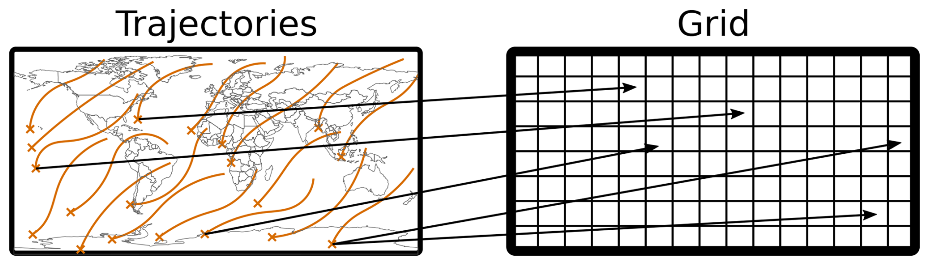
Figure 2 Visual representation of a mapping, each trajectory is assigned to some grid points based on their initial position, note that for visual clarity only some mappings are drawn. The way in which this association is done forms an integral part of our pipeline and is based on solving a minimal weight full bipartite matching problem.

While creating such an initial association can be done trivially, there are constraints that make the task more difficult. The first and most crucial constraint is that the resulting grids need to be smooth. Secondly, we must ensure that every trajectory maps to at least one grid point. If this is not the case, a trajectory would have no representation in the compressed data and would therefore be lost during compression. These constraints, especially the smoothness one, prevent the use of naive mapping methods and require the use of more sophisticated techniques.

In our research, we analysed different mapping methods. The one that yields the best results is based on solving a minimal weight full bipartite matching problem, originating in graph theory (Burkard et al., 2012). A second promising approach is based on solving a linear program (LP) (Bertsimas and Tsitsiklis, 1997). Solving this LP becomes computational infeasible for large images, but we still include it for theoretical analysis.

2.2.1 Bipartite Mapping

For this mapping method (results in Fig. 3, with an example in Fig. 4), the problem is solved using concepts from graph theory, more specifically by solving a minimal weight full bipartite matching problem. Hence, following this approach, we have two sets of nodes: one called “workers” and the other called “tasks”, with weighted edges between them constraining which workers may be assigned to which tasks and what the cost of this assignment is. The goal is to match each worker to exactly one task while trying to keep the overall cost of the matchings as low as possible.

Figure 3 Latitude grids with 550 hPa starting pressure created with the bipartite mapping method. Three different time steps are displayed the leftmost image is at the first time step, the second one is 12 h later and the rightmost one is 24 h later. In the leftmost image we have very good smoothness, which originates from the mapping method, over time this smoothness starts to degrade, as the trajectories start to diverge.

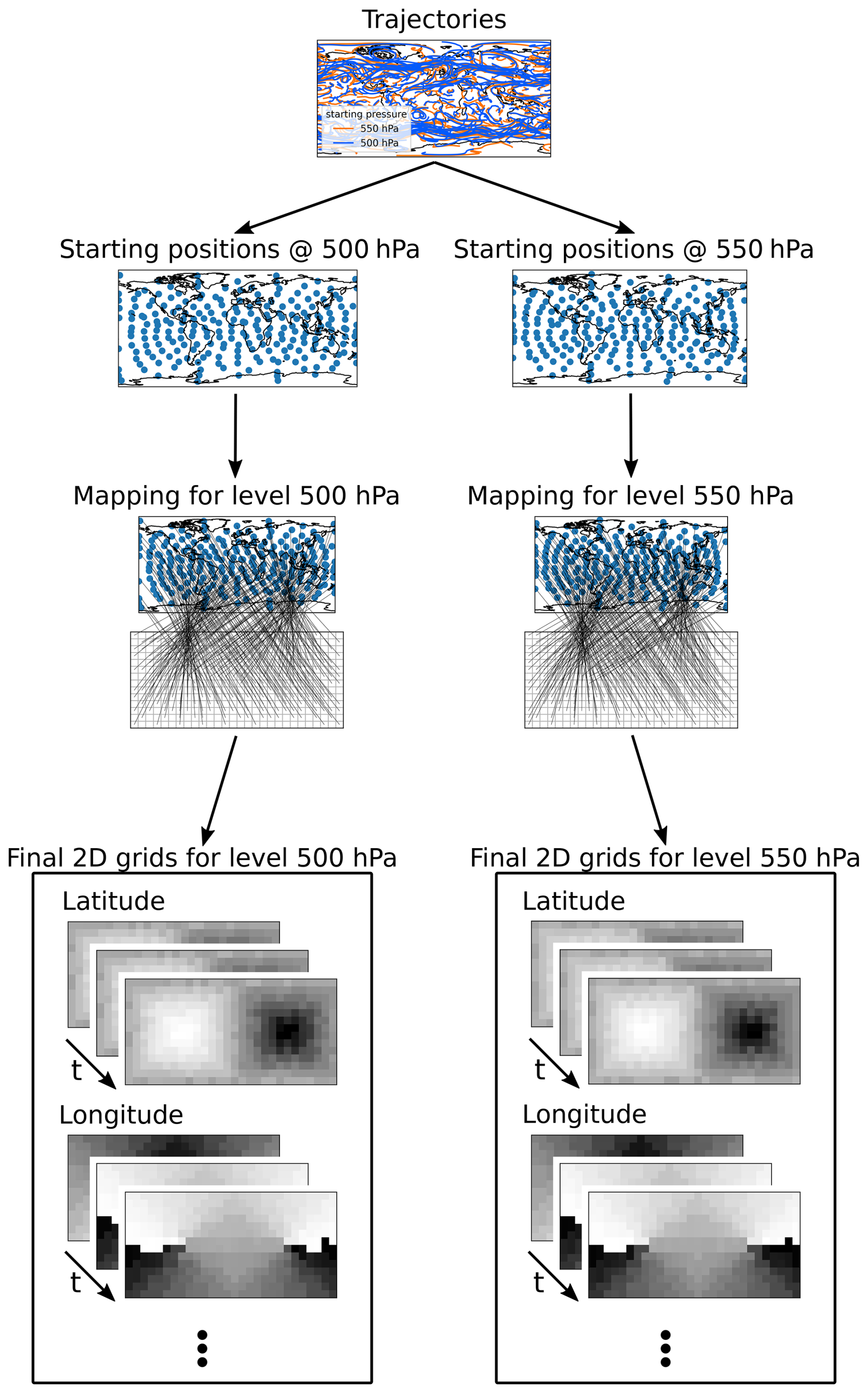
Figure 4 Example of how the bipartite mapping works. For this 464 trajectories starting at two different pressure levels are considered. In a first step we extract the staring positions of all the trajectories individually for the two different pressure levels. We then take these starting positions and create a mapping to a grid such that the resulting grids are smooth. This mapping is then used to generate a collection over time for each of the data variables which are present on our trajectories.

This minimum weight full bipartite matching problem can be easily applied to our use case. Namely, the workers become the trajectories and the tasks the grid points. The weights are then defined as the Euclidean distance between the trajectories and the grid points at the first time step after both are translated into 3D Cartesian space. To transform the grid points into Cartesian space, a projection onto a 3D sphere is used. This projection method should lead to the grid points being homogeneously distributed over the globe, making a simple longitude-latitude mapping unsuitable. We chose the projection presented in Sect. 4 of the paper by Calhoun et al. (2008). The trajectories are transformed into Cartesian space by taking their spherical coordinates of longitude, latitude, and pressure and converting them to Cartesian x, y, and z coordinates. This transformation leads to the creation of a spherical shell, representing a mismatch in dimensionality between the grid points and the trajectories. Therefore, the spherical shell is binned into discrete levels over its pressure, resulting in the creation of multiple spheres for each of the bins. This means that, in addition to a grid being created for each time step and data variable, individual grids are also created for each of these pressure levels. If the algorithm then minimizes the Euclidean distance between the trajectories and the grid points, the resulting grids should become smooth, as trajectories with similar starting positions should be mapped to grid points that are close to one another, and we have that trajectories starting at similar spatial positions behave rather similarly over time (hence locating them next to each other results in a smoother grid). So, by representing our mapping problem as such a graph problem and solving it, we should end up with a valid and smooth mapping.

One problem with this mapping via minimal weight full bipartite matching is that if the number of trajectories is less than the number of grid points some grid points will not be mapped, leading to holes in the resulting grid. While it theoretically is possible to have the same number of trajectories as grid points, tests showed that this can become computationally infeasible and that in practice we need more grid points than trajectories. Therefore, we need to devise a way to handle this. The hole filling works by taking all the grid points that do not get mapped and mapping their closest trajectory (Euclidean distance in Cartesian space) to them (note that this means that a trajectory may map to multiple grid points at the same time). By using this method, the holes can be filled in an easy manner that does not require any costly computations.

2.2.2 LP Mapping

We also considered using linear programming. While this approach has high theoretical appeal, its practical usability is limited by the fact that the resulting LP becomes very large and requires a lot of resources to solve, while delivering nearly identical results to the approach based on minimal weight full bipartite matching. For our use case, we will model the mapping problem as an integer linear program (ILP), for which we then show that its LP formulation is integral, i.e., solving the LP formulation instead of the ILP one delivers the same results. This allows us to use a much cheaper LP solver, resulting in a large decrease in computational resources. In order to define an integer linear program, we need to specify an objective and a set of constraints that create a valid and smooth mapping from trajectories to grid points.

We first start with an intuitive definition of the objective and the constraints. The objective function is designed to minimize the sum of distances between the trajectories and their associated grid points. For the constraints, we say that each trajectory must map to at least one grid point and that each grid point must be mapped to. By the property of spatial continuity, a minimization of the objective function should lead to a smooth grid, while the constraints ensure that the mapping is valid. The rigorous mathematical definition is then given by:
Let the binary variables $x_{t,p}\in \mathit{\{}\mathrm{0},\mathrm{1}\mathit{\}}$ denote whether a trajectory t∈T is mapped to grid point p∈P, 0 if not mapped, 1 if mapped. And let the variable $d_{t,p}\in {\mathbb{R}}_{\ge \mathrm{0}}$ denote the Euclidian distance in 3D Cartesian space (defined analogue to the bipartite mapping method) between a trajectory t∈T and a grid point p∈P. The resulting ILP is then given in Eq. (1):

$$\begin{array}{}\text{(1)}& {\displaystyle }\text{minimize}\sum _{(t,p)\in T\times P}{d}_{t,p}{x}_{t,p}\text{(2)}& {\displaystyle }\begin{array}{r}\text{s.t.}\sum _{t\in T}{x}_{t,p}=\mathrm{1}\forall p\in P\\ \sum _{p\in P}{x}_{t,p}\ge \mathrm{1}\forall t\in T\end{array}\end{array}$$

While the variables x_t,p are defined to be binary, making the problem an integer LP, we can prove (see Appendix A) that the LP formulation, achieved by defining $x_{t,p}\in [\mathrm{0},\mathrm{1}]$, is integral. This means that instead of an ILP solver a much cheaper LP solver can be used during calculation.

2.3 Color Encoding

To motivate color encoding, we must examine the longitude grids created by the previously explored mappings (Fig. 5 top), which mapping we look at (LP or bipartite) is not important as they deliver very similar results. As we can see from Fig. 5 top, there is a discontinuity line around the position of the dateline at longitude 180°, which begins to warp as time progresses. This discontinuity arises because trajectories with a longitude value of −180 (black pixels) are adjacent to trajectories with longitude values of 180 (white pixels). Such jumps in pixel values lead to worsened compression performance, as shown by experiments where we observed a decrease in RMSE error in the longitude variable by a factor of 1.4 when compressing with color encoding compared to no color encoding (using a compression factor of 15).

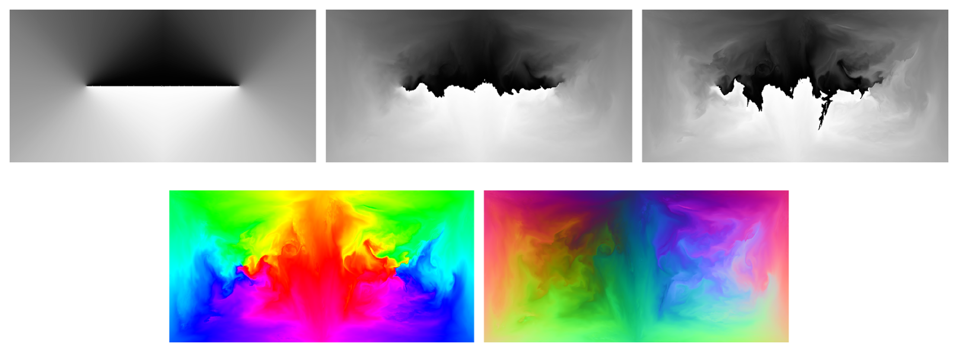
Figure 5 Top: Longitude grids with 550 hPa starting pressure displayed over different time steps (0, 12, 24 h). At the date line there is a discontinuity which starts to warp over time. This discontinuity leads to worsened compression performance and we can use color encoding to fix this. Bottom: HSV (left) and XYZ (right) color encoded longitude grids with 550 hPa starting pressure displayed after 24 h. The date line discontinuity is gone.

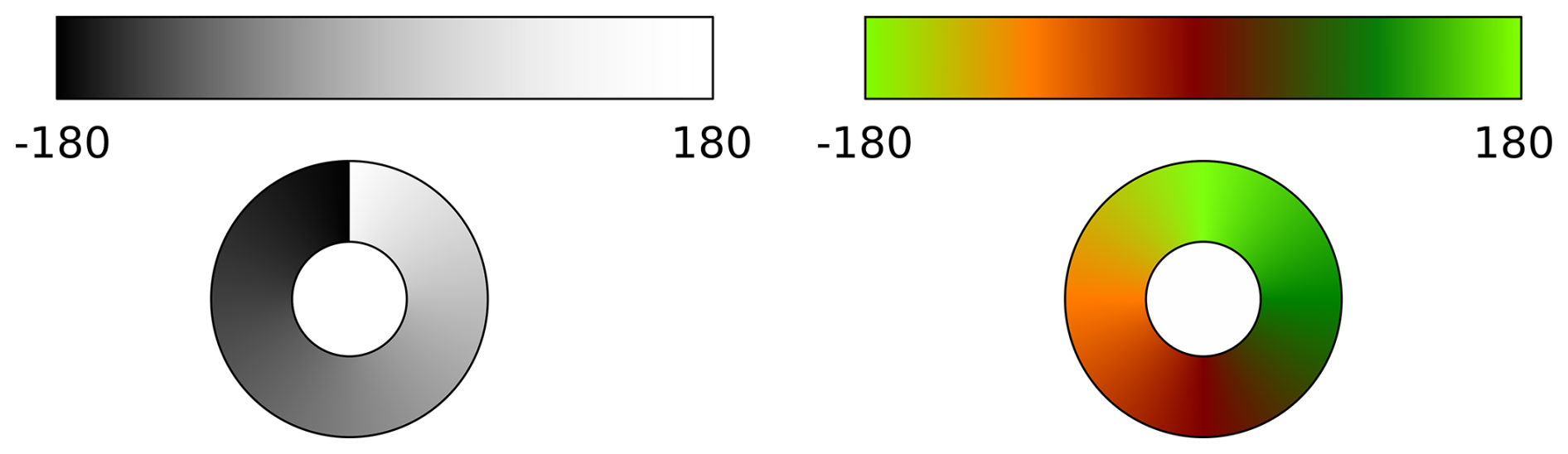
Figure 6 Qualitatively demonstration of the discontinuity line at the date line. On the left only a singular variable (black to white) is used to represent the longitude, a discontinuity is created. On the right two variables and a cosine sine mapping is used, displayed as red and green. Using two variables it is possible to create a continuous color cycle with no discontinuity.

The way we eliminate the discontinuity line is by using multiple variables instead of one, which maps the $[-\mathrm{180},\mathrm{180}]$ longitude range to the black to white pixels. Hence, we map the $[-\mathrm{180},\mathrm{180}]$ to a multidimensional space. If we use two or three variables, this multidimensional space can be represented by a color bar. This concept is illustrated in Fig. 6, where on the left, we have a single variable mapping the longitude from black to white, generating a discontinuity in the color wheel. On the right, we use two variables (red and green) with a sine-cosine mapping to create a color bar, which results in a continuous color wheel. This simple concept can define a variety of different color encoding methods. In our research, we explored several such methods, and the ones that provided the best performance are based on utilizing three variables, covering the entire RGB range. We call them HSV and XYZ color encoding and they are explained in the following sections.

2.3.1 HSV color encoding

The HSV color encoding method (Fig. 5 bottom left) uses the HSV (Smith, 1978) color representation, which, like RGB, is a way to describe color. However, instead of using values for red, green, and blue, it uses hue, saturation, and value to represent color. For our use case, we set the saturation and value to 1 and only vary the hue. For constant saturation and value, a varying hue generates a continuous color wheel. Another reason for setting saturation and value to 1 is that the JPEG 2000 algorithm might handle dark or washed-out colors differently, as the human eye cannot distinguish them as precisely as strong, bright colors.

The function f(x) for converting a longitude value in the normalized range [0,1] to an RGB value using an HSV representation is given in Eq. (3). The inverse mapping $f_{\text{inv}}\left(\right[r,g,b{]}^T)$, which maps an RGB color value to a hue angle, is provided in Eq. (4).

$$\begin{array}{}\text{(3)}& {\displaystyle }\begin{array}{rl}& f\left(x\right)=\left[\begin{array}{c}h\left(\mathrm{5}\right)\\ h\left(\mathrm{3}\right)\\ h\left(\mathrm{1}\right)\end{array}\right]\\ & \text{with}\\ & h\left(l\right)=\mathrm{1}-max\left\{\mathrm{0},min\left\{k,\mathrm{4}-k,\mathrm{1}\right\}\right\}\\ & k=(l+\mathrm{6}x)\mathrm{mod}\mathrm{6}\end{array}\text{(4)}& {\displaystyle }\begin{array}{rl}& f_{\text{inv}}\left(\right[r,g,b{]}^T)=\left\{\begin{array}{ll}\mathrm{0},& \text{if }c=\mathrm{0}\\ \frac{\mathrm{1}}{\mathrm{6}}\cdot \left(\frac{g-b}{c}\mathrm{mod}\mathrm{6}\right),& \text{if }v=r\\ \frac{\mathrm{1}}{\mathrm{6}}\cdot \left(\frac{b-r}{c}+\mathrm{2}\right),& \text{if }v=g\\ \frac{\mathrm{1}}{\mathrm{6}}\cdot \left(\frac{r-g}{c}+\mathrm{4}\right),& \text{if }v=b\end{array}\right.\\ & v=max\left\{r,g,b\right\}\\ & k=min\left\{r,g,b\right\}\\ & c=v-k\end{array}\end{array}$$

2.3.2 XYZ color encoding

The XYZ color encoding (Fig. 5 bottom right) method considers both the longitude and latitude data variables, combining them into a single three-channel color grid. To this end, the longitude and latitude values are taken and converted into Cartesian coordinates, from which the r, g, b color channels are created from the x, y, z positional coordinates.

The function f([x_lon,x_lat]^T), which maps both longitude and latitude in the normalized range [0,1] to RGB values, is given in Eq. (5). The inverse function $f_{\text{inv}}\left(\right[r,g,b{]}^T)$, which converts RGB values back to longitude and latitude, is given by Eq. (6).

$$\begin{array}{}\text{(5)}& {\displaystyle }\begin{array}{rl}& f\left(\right[x_{\text{lon}},x_{\text{lat}}{]}^T)={\displaystyle \frac{\mathrm{1}}{\mathrm{2}}}\left(\mathrm{1}+\left[\begin{array}{c}\cos {\widehat{x}}_{\text{lat}}\cos {\widehat{x}}_{\text{lon}}\\ \cos {\widehat{x}}_{\text{lat}}\sin {\widehat{x}}_{\text{lon}}\\ \sin {\widehat{x}}_{\text{lat}}\end{array}\right]\right)\\ & \text{where }{\widehat{x}}_{\text{lat}}=\mathit{\pi }(x_{\text{lat}}-{\displaystyle \frac{\mathrm{1}}{\mathrm{2}}}),{\widehat{x}}_{\text{lon}}=\mathrm{2}\mathit{\pi }(x_{\text{lon}}-{\displaystyle \frac{\mathrm{1}}{\mathrm{2}}})\end{array}\text{(6)}& {\displaystyle }\begin{array}{rl}& f_{\text{inv}}\left(\right[r,g,b{]}^T)=\left[\begin{array}{c}\frac{\mathrm{1}}{\mathrm{2}\mathit{\pi }}\left(\text{arctan2}\right(\widehat{g},\widehat{r})+\mathit{\pi })\\ \frac{\mathrm{1}}{\mathit{\pi }}\left(\text{arctan2}\right(\widehat{b},\sqrt{{\widehat{r}}^{\mathrm{2}}+{\widehat{g}}^{\mathrm{2}}})+\frac{\mathit{\pi }}{\mathrm{2}})\end{array}\right]\\ & \text{where }\widehat{r}=\mathrm{2}r-\mathrm{1},\widehat{g}=\mathrm{2}g-\mathrm{1},\widehat{b}=\mathrm{2}b-\mathrm{1}.\end{array}\end{array}$$

2.4 Delta Encoding

We also looked into using delta encoding as part of our compression pipeline. The principle behind delta encoding is that instead of storing time sequenced data directly, the delta between subsequent time steps is calculated and saved. While the calculation of the delta itself will not lead to a decrease in data, it might reduce entropy, which can beneficially impact the performance of compression algorithms. We will formulate this more rigorously in the rest of this section.

We will start with a naive implementation of delta encoding and show that it is not suitable. We will use the following notation: At time step i, the full grid is denoted as g_i, and the delta between the grids at time steps i and i−1 is denoted as Δ_i. It is calculated by subtracting the previous grid from the current one: ${\mathrm{\Delta }}_i=g_i-g_{i-\mathrm{1}}$. Then, instead of passing the full grid sequence $(g_{\mathrm{1}},g_{\mathrm{2}},\mathrm{\dots },g_N)$ to the dense data compressors, we use the delta sequence $(g_{\mathrm{1}},{\mathrm{\Delta }}_{\mathrm{2}},{\mathrm{\Delta }}_{\mathrm{3}},\mathrm{\dots },{\mathrm{\Delta }}_N)$. The problem with this simple delta encoding approach is that the error starts to accumulate over time. To see this, we define

$$\begin{array}{}\text{(7)}& {\displaystyle }{g}_i^{\prime }=g_i+{\mathit{ϵ}}_i\text{(8)}& {\displaystyle }{\mathrm{\Delta }}_i^{\prime }={\mathrm{\Delta }}_i+{\mathit{\eta }}_i=g_i-g_{i-\mathrm{1}}+{\mathit{\eta }}_i\end{array}$$

as the full frames and the delta frames which have gone though compression and therefore have an error ϵ_i and η_i applied to them. The grid at time step i that gets reconstructed by this is:

$$\begin{array}{}\text{(9)}& g_i^r=g_{\mathrm{1}}^{\prime }+\sum _{j=\mathrm{2}}^i{\mathrm{\Delta }}_j^{\prime }=g_i+{\mathit{ϵ}}_{\mathrm{1}}+\sum _{j=\mathrm{2}}^i{\mathit{\eta }}_j\end{array}$$

Therefore the delta frame compression errors η_j start to accumulate over time. We can solve this problem rather easily. Instead of defining a delta frame from the “perfect” grid g_i−1, we use the reconstructed $g_{i-\mathrm{1}}^{r*}$ grid:

$$\begin{array}{}\text{(10)}& \begin{array}{rl}& {{\mathrm{\Delta }}^{\prime }}_i^{*}={\mathrm{\Delta }}_i^{*}+{\mathit{\eta }}_i=g_i-g_{i-\mathrm{1}}^{r*}+{\mathit{\eta }}_i,\\ & g_{i-\mathrm{1}}^{r*}=g_{\mathrm{1}}^{\prime }+\sum _{j=\mathrm{2}}^{i-\mathrm{1}}{{\mathrm{\Delta }}^{\prime }}_j^{*}\end{array}\end{array}$$

The $g_i^{r*}$ can then be reformulated to

$$\begin{array}{}\text{(11)}& g_i^{r*}=g_{\mathrm{1}}^{\prime }+\sum _{j=\mathrm{2}}^i{{\mathrm{\Delta }}^{\prime }}_j^{*}=g_i+{\mathit{\eta }}_i\end{array}$$

As we can see here the error does not start to accumulate over time, therefore this method is to be preferred over the naive one.

2.5 Implementation details

For the implementation, we had to take certain shortcuts and make adjustments to the theory in order to remain within reasonable computational limits. The primary simplification we made was to limit the possible number of grid points a trajectory may map to, for both the bipartite and the LP mapping, to a set of its closest neighbors. For bipartite mapping, this was the closest 200 neighbors, while for the LP mapping, it was the closest 50. However, this introduces the additional constraint of needing the starting locations of the trajectories to be evenly distributed. If they are not evenly distributed, i.e., if there are regions of low and high trajectory density, the mapping phase will fail, as we reach a point where we have locally more trajectories than possible grid points to which they may map. How limiting this constraint is depends on the type of research. For some studies, the initial configuration is uniform, e.g., a global uniformity in Stoffels et al. (2025) Sprenger et al. (2017), and Bakels et al. (2025) or local uniformity in Pérez-Muñuzuri et al. (2018), and Wendisch et al. (2024). But there is also research such as Keune et al. (2022), Schielicke and Pfahl (2022), and Dey et al. (2023) where non-uniform initial configurations are used and which therefore cannot be handled by psit. A second shortcut we are taking is that we need more grid points than trajectories in practice, this is due to both considering only the closest neighbors and because the algorithmic implementation we chose to solve the minimal weight full bipartite matching problem performs much faster when there are more grid points compared to trajectories. In practice, we have around 50 % more grid points than trajectories. These are the main considerations we had to take during implementation in order to strike a balance between computational performance and compression capabilities. In the future, it might be advisable to revisit these shortcuts, as removing them could lead to a broader applicable field of psit.

Some other minor implementation details are that we only implemented color encoding in combination with the JPEG 2000 compression algorithm, and that when compressing local rather than global trajectories (i.e., starting positions are bounded inside a box instead of spanning the entire globe), a longitude-latitude projection is used to map the grid points into 3D Cartesian space. This is because there is no simple inverse function for the presented projection method. Both of these differences do not have a large impact on the compression performance of psit, but could still be explored in future research.

3 Results

Previous research (Baker et al., 2014, 2016; Poppick et al., 2020) has already shown that simple error metrics are not enough to argue about the effectiveness of lossy compression algorithms in the case of weather and climate data. Therefore in this section we explore a set of experiments which should cover a range of different metrics and should give a general overview of how psit performs. In total we will carry out five different experiments:

1. Error metrics and comparison to ZFP (pyzfp v0.5.5) and SZ3 (v3.2.1) in order to compare performance to existing alternatives,

2. error value distribution in order to discern the creation of bias in the error,

3. trajectory density comparison against trajectories produced from perturbed wind fields in order to compare the impact of compression with the impact of data assimilation inaccuracies,

4. two case studies, one about warm conveyor belts and one about the Fukushima disaster, in order to see how psit performs in a more realistic environment,

5. and throughput and memory usage to observe the computational performance.

This should provide the reader with an insight into how psit behaves in different situations.

3.1 Input Data

Table 1 The minimal and maximal values for the different data variables of the tra_20200101_00 file.

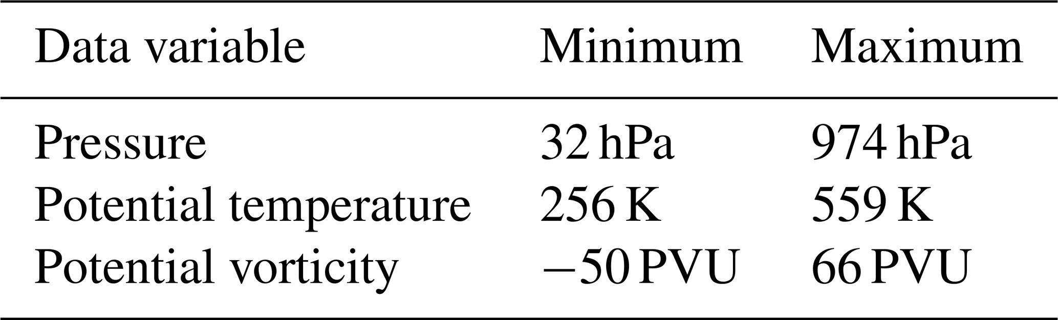
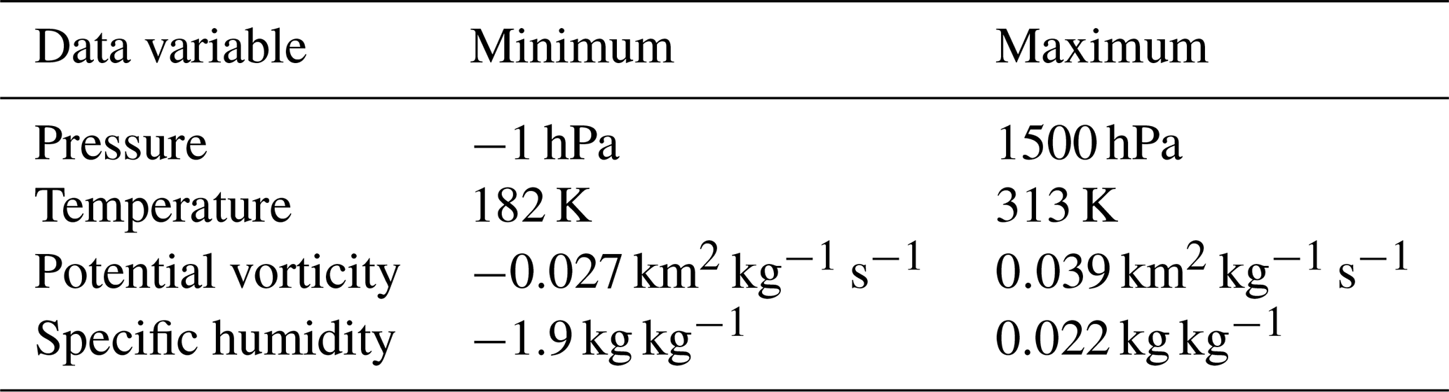
Table 2 The minimal and maximal values for the different data variables of the tra_20200101_00 file.

During the following experiments we will use the following trajectory files:

• tra_20200101_00. A file produced using Lagranto (Wernli and Davies, 1997a; Sprenger and Wernli, 2015), based on ERA5, starting on 1 January 2020, 00:00 UTC and going until 2 January 2020, 00:00 UTC, with a total of 13 time steps (each two hours long). It consists of 5 289 105 trajectories, distributed across 26 pressure levels at the first time step with horizontal spacing of 50 km, and vertically ranging from 50 to 550 hPa in 20 hPa increments. The additional data variables (ranges given in Table 1) it stores are potential temperature (TH) and potential vorticity (PV). The file is 1.3 GB in size.

• tra_20200101_00_permuted. This is the same trajectory file as tra_20200101_00, but with the trajectory order randomly permuted. Everything else remains the same. The order of the trajectories in the tra_20200101_00 dataset follows the grid and pressure levels, which leads to continuity (i.e., neighbouring trajectories are similar) if the trajectories are traversed in order. By permuting them, this continuity is removed.

• tra_20000101_00. A trajectory file produced using Lagranto, based on ERA5, starting on 1 January 2000, 00:00 and extending 168 h until 8 January 2000 01:00. It consists of 5 867 016 trajectories distributed over the default 37 ERA5 pressure levels from 1000 to 1 hPa, with spacing of 40 km. The additional data variables traced along the trajectories are (ranges given in Table 2) temperature (T), potential vorticity (PV), and specific humidity (Q). The file is 23 GB in size.

• tra_20000101_00_permuted. The same trajectory file as tra_20000101_00, but with the trajectory order randomly permuted. The reasoning behind this is the same as for the tra_20200101_00_permuted file.

3.2 Performance of psit

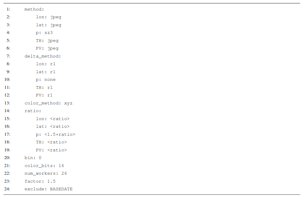
Listing 1 Configuration file for psit used for the runs presented in Sect. 3.2. The compression ratios are replaced by placeholders <ratio> to indicate that they are changed between the different runs, the compression ratio for the pressure variable is 1.5 larger than for the other ones.

Table 3 Ablation study for psit on the tra_20200101_00 trajectory file. For different configurations the file is compressed to a compression ratio of around 20 after which the RMSE error for the different data variables is considered. If we then pick the lowest value for each error column we can figure out the optimal configuration. It consists of using JPEG 2000 with delta encoding for all data variables except pressure where SZ3 with no delta encoding should be used, additionally we should use XYZ color encoding. The lowest value is always highlighted in a bold font.

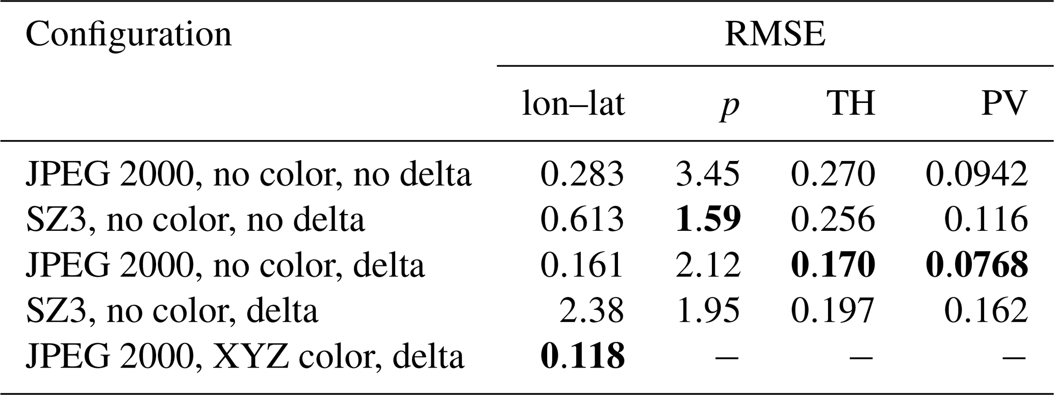
There are different ways in which psit can be configured, leading to different compression behaviors. Here, we present one configuration stack that led to good results with the presented input data files. We found this optimal configuration by performing an ablation study in which we run psit in different configurations and then combine the best performing parts together. A summary of this can be seen in Table 3, where we compress the tra_20200101_00 file in different configurations, but always with a ratio of around 20. We then look at the RMSE error of the different data variables in order to figure out what the best configuration is. In this configuration we are using the JPEG 2000 compression algorithm combined with delta encoding for every data variable except for pressure, where we use SZ3 (v3.2.1) with no delta encoding. Additionally, we utilize the XYZ color encoding scheme. This configuration is given by the configuration file in Listing 1, for a description of how these configuration files work, please refer to the user manual at (Pietak, 2025a). The compression factor, a metric that determines how strong the compression should be, is varied between the different runs and is the same for every data variable except for pressure, where it is 1.5 times larger. We will use this configuration for all of the following experiments, except for the case study on the Fukushima disaster, as we are working with a different input file there.

3.2.1 Error metrics and comparison with ZFP and SZ3

In this experiment, a comparison between compression ratio and compression error for psit, ZFP, and SZ3 is conducted. The compression pipeline for ZFP works by treating each data variable as a 2D array over the time steps and the trajectories and compressing each of them individually, for ZFP we are using pyzfp v0.5.5 in fixed-accuracy mode. The pipeline for SZ3 is identical to the one used for ZFP, we are using the python interface pysz, version 3.2.1 and are running in the relative error bound mode. The error norms we use in this study are the L1, RMSE, L-infinity errors and the peak signal to noise ratio (PSNR) between the original and the compressed/decompressed data, which are obtained by calculating the errors defined by Eqs. (12), (13), (14), and (15) between each data variable of the original and compressed/decompressed data file.

$$\begin{array}{}\text{(12)}& {\displaystyle }{l}_{\mathrm{1}}={\displaystyle \frac{\mathrm{1}}{n}}\sum _{i=\mathrm{1}}^n|x_i-y_i|\text{(13)}& {\displaystyle }{l}_{\text{rmse}}=\sqrt{{\displaystyle \frac{\mathrm{1}}{n}}\sum _{i=\mathrm{1}}^n(x_i-y_i{)}^{\mathrm{2}}}\text{(14)}& {\displaystyle }{l}_{\mathrm{\infty }}=\underset{i=\mathrm{1},\mathrm{\dots },n}{max}\mathit{\left\{}\right|x_i-y_i\left|\mathit{\right\}}\text{(15)}& {\displaystyle }{l}_{\text{psnr}}=\mathrm{20}{\log }_{\mathrm{10}}\left(d\right)+\mathrm{20}{\log }_{\mathrm{10}}\left(l_{\text{rmse}}\right)\end{array}$$

where n is the number of data points, x the original data, y the compressed/decompressed data and d the extent of the data. As we are using color encoding, we need to handle the longitude and latitude variables differently. Instead of using the difference, we use the central angle between the input and the output (defined as the angle on a great circle between two points on a sphere). The amount of compression error and therefore the compression ratio that is acceptable depends on the case in which the data is used. We therefore provide a wide range of compression ratios such that the reader is able to evaluate the general behavior and then based on this figure out what compression ratios are well suited for their needs. Such a comparison between psit and the other methods provides us with an overview of how psit compares to already existing alternatives and therefore allows us to assess its viability.

In the first run, the tra_20200101_00 and tra_20200101_00_permuted files are considered. An excerpt of this can be seen in Fig. 7, with the full plots given in Fig. B1 and a normalized version in Fig. B2 and the exact values in Tables B1, B2, B3, B4, and B5. When looking at both ZFP and SZ3, we see that the performance between the different input data files differs significantly. The performance of the permuted trajectory file is much worse compared to the non permuted one. This is because, for the tra_20200101_00 file, the trajectories have been initialized on an equidistant grid and are stored in the file in an ordered manner. Therefore, by converting them into the 2D grids over time steps and trajectories, a naive smoothness (originating from spatial continuity) of the grid is created. When we permute the trajectories, this naive smoothness is destroyed, and the compression performance drops. This means that the compression performance of ZFP and SZ3 does not only depend on the data, but also on the way in which it is stored, something from which psit does not suffer. This also makes it difficult to predict and quantify the behavior of ZFP and SZ3 on input files. Comparing them with psit we see that psit gives consistent results independent on the input file. In the smaller compression range psit does not perform as well, this could be because during the mapping phase artificially more points are added. We also see that in general psit performs worse for pressure than it does for lon–lat this data variable dependent performance is something we quite often see.

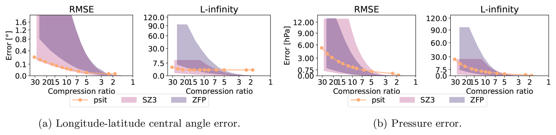
Figure 7 Excerpt of the comparison between psit, ZFP, and SZ3 for the tra_20200101_00 and tra_20200101_00_permuted files. The configuration of our program is described in Sect. 3.2 and the corresponding config file is given in Listing 1. The RMSE and L-infinity error is compared to the achieved compression ratio for the central angle error (lon–lat) and pressure (p). In the plots the shaded area for ZFP and SZ3 corresponds to the range in compression performance between the two files. Note that psit performs the same for both, therefore, only one line is plotted.

In the second run, we consider the tra_20000101_00 and tra_20000101_00_permuted files. This can be seen in Fig. B3 normalized version in Fig. B4, with exact values given in Tables B6, B7, B8, B9, and B10. For psit against ZFP we observe a similar, though less pronounced, behavior. Now, the difference between the two compression methods is less distinct, and psit only starts to perform better than ZFP for larger compression ratios. The performance of SZ3 now looks better and it outperforms psit for some cases. This decrease in performance for this larger trajectory file indicates that psit, in general, struggles with longer time ranges. A reason for this could be that over time, trajectories start to diverge, and therefore, the smoothness in the images, which is based on their initial position, gets lost (see e.g., Fig. 3).

From the above observations, we can make some general statements about the performance of psit. For smaller time ranges, psit performs on par with or better than ZFP and SZ3, with a notable exception being the pressure variable, due to its inherent noisy behavior. For longer time ranges, the performance of psit starts to degrade. Additionally, for cases where keeping a small L-infinity error is important, we should use SZ3 over JPEG 2000, as it bounds the L-infinity error. Moreover, the performance of ZFP and SZ3 is highly dependent on the way the input data is structured, something from which psit does not suffer. We therefore conclude that psit is a viable alternative to ZFP and SZ3, and can deliver consistent results.

3.2.2 Error Value Distribution

The next experiment we are conducting is about the error distribution. For this, we compress the tra_20200101_00_permuted and tra_20000101_00_permuted files with psit, ZFP, and SZ3 and compression ratios of around 2.5, and 15, then calculate the difference from the original file and put normalized versions of these differences into a histogram. We chose these compression ratios as they represent both a small and a somewhat medium compression ratio. Based on the shape of the corresponding histogram we then can gauge if bias is introduced by the compression.

The distribution for the tra_20200101_00_permuted file is shown in Fig. 8, while the one for the tra_20000101_00_permuted is given in Fig. B5. For all variables we have that for psit the mean is nearly perfectly at 0. We also have that the shape for psit tends to be very similar over the different compression ratios. The other compression methods mostly also manage to keep the mean at zero, but tend to have vastly different (often non-smooth) shapes especially for the higher compression ratios. This indicates that psit generally does not introduce a bias.

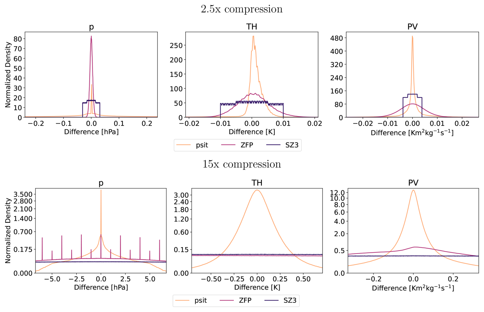
Figure 8 Area-normalized error distribution based on values for the tra_20200101_00_permuted dataset using the compression setup for psit of Sect. 3.2. We compress with compression ratios of 2.5, and 15. The area of the densities have been normalized and the x axis is cropped to 5 standard deviations of the psit distribution for all cases, except pressure with 2.5 times compression where it is 1 standard deviation. The data variables are pressure (p), potential temperature (TH), and potential vorticity (PV).

3.3 Trajectory Density and Comparison to Perturbed Wind Fields

In this experiment, we examine the impact compression has on the position of the trajectories over time. To examine this impact, we calculate the densities of the trajectories starting at different pressure levels (1, 500, 1000 hPa) for increasing time steps (72, 120, 168 h). In addition to comparing uncompressed and compressed trajectories, we also look at uncompressed trajectories calculated from perturbed wind fields, simulating the impact of measurement uncertainties. In total, we consider the following trajectory datasets:

• Uncompressed trajectories,

• the tra_20000101_00 trajectory file compressed with psit for compression ratios of 1.67, 12.8, 44.5,

• uncompressed trajectories (similar to tra_20000101_00) calculated from wind fields to which uniform noise to the horizontal/vertical components of magnitudes $\mathrm{0.01}\mathrm{m}{\mathrm{s}}^{-\mathrm{1}}/\mathrm{6.67}\times {\mathrm{10}}^{-\mathrm{4}}$ Pa s⁻¹, $\mathrm{0.05}\mathrm{m}{\mathrm{s}}^{-\mathrm{1}}/\mathrm{3.33}\times {\mathrm{10}}^{-\mathrm{3}}$ Pa s⁻¹, and $\mathrm{0.1}\mathrm{m}{\mathrm{s}}^{-\mathrm{1}}/\mathrm{6.67}\times {\mathrm{10}}^{-\mathrm{3}}$ Pa s⁻¹ has been added.

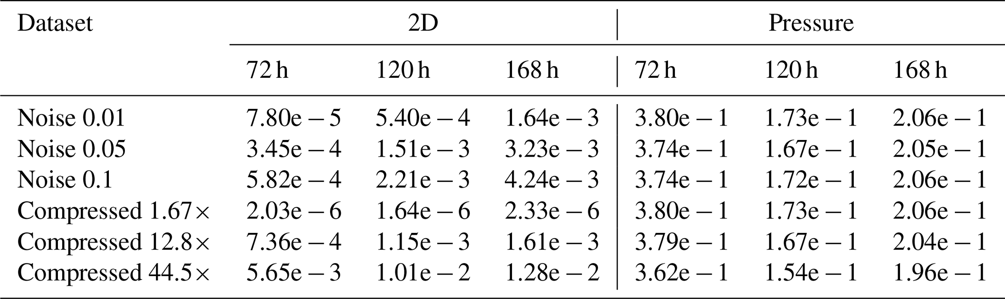
The compression ratios are chosen in a way such that the entire range of compression ratios explored in Sect. 3.2.1 is covered. We then calculate 2D densities over longitude and latitude (number trajectories over given area), and 1D densities over pressure (number trajectories over given pressure range), for which we consider the Jensen–Shannon divergence. We calculate the Jensen–Shannon divergence for the 2D case by partitioning the globe into equally sized bins and counting the number of trajectories per bin, and for the 1D case by using a histogram. This can be seen for example in Fig. 9. Such a density comparison between these different datasets and the uncompressed one allows us to see the impact compression has on the trajectory positions and also how compression behaves compared to perturbed wind fields.

The Jensen–Shannon divergence is shown in Tables B11, B12, and B13. From the tables, we can see that over time, the errors start to increase. The same (unsurprisingly) also holds for increasing compression ratio and perturbation magnitude. Furthermore, the error in pressure for the 500 and 1000 hPa pressure levels tends to be large and very similar between all runs, indicating that it is a very sensitive metric, as any perturbation leads to large errors. For the 2D divergence metric, we find that with psit compressed trajectories in the compression range of 12.8 to 44.5 behave very similarly to perturbed wind fields with perturbation magnitudes of $\mathrm{0.05}\mathrm{m}{\mathrm{s}}^{-\mathrm{1}}/\mathrm{3.33}\times {\mathrm{10}}^{-\mathrm{3}}$ to $\mathrm{0.1}\mathrm{m}{\mathrm{s}}^{-\mathrm{1}}/\mathrm{6.67}\times {\mathrm{10}}^{-\mathrm{3}}$ Pa s⁻¹. The lowest compression ratio of 1.67 tends to outperform all the perturbed wind fields. This experiment demonstrates that psit behaves very similarly to perturbed wind fields, showing that the error incurred by compression lies within inaccuracies generated by data assimilation techniques.

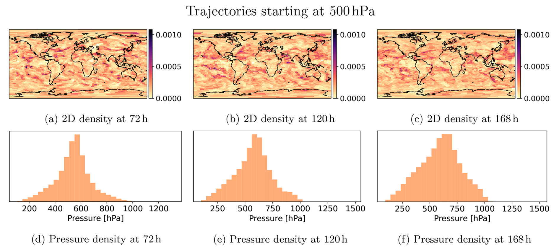
Figure 9 Reference image for how we calculate both the 1D and the 2D densities. For this we consider trajectories staring at at 500 hPa and calculate the densities over multiple time steps. The 2D density is given over longitude and latitude, and as a 1D density over pressure.

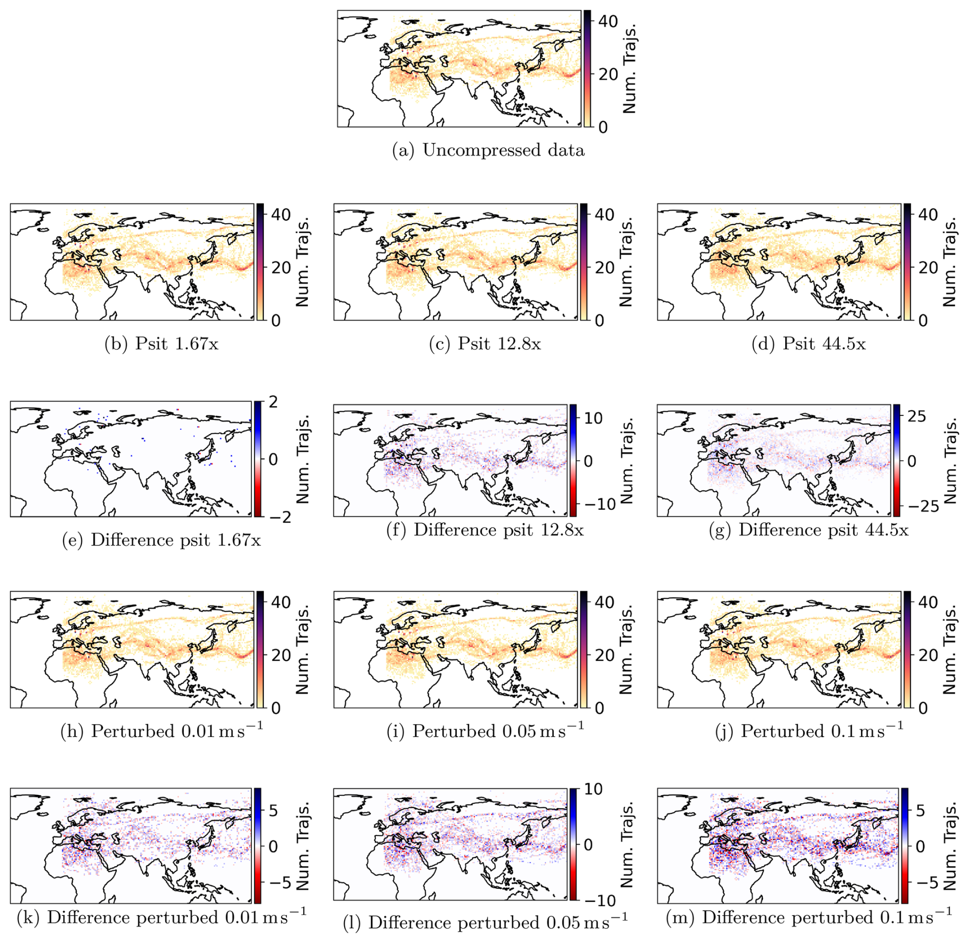
Figure 10 Comparison of the densities of trajectories starting in the box from 0 to 15° E times 45 to 60° N after 168 h. The trajectories we consider are uncompressed trajectories, compressed trajectories and trajectories calculated from perturbed wind fields.

Instead of looking at global trajectory densities, we can also look at local ones. For this, we take all the trajectories starting in the box from 0 to 15° E and 45 to 60° N, and plot their density alongside the difference to the uncompressed trajectories after 168 h (Fig. 10). From these plots, we can see that the general features are preserved under compression and that compression behaves very similarly to adding random perturbations to the wind field, again confirming that psit and perturbed wind fields lead to similar behavior of the trajectories.

3.4 Case Studies

3.4.1 Warm Conveyor Belts

The Warm Conveyor Belt (WCB) is one of three characteristic air streams in extratropical cyclones (Browning et al., 1973; Madonna et al., 2014). WCBs ascend in the cyclones' warm sector from the boundary layer to upper-tropospheric levels. This ascent, which occurs within 48 h and extends over 600 hPa, is associated with substantial cloud and precipitation formation (Pfahl et al., 2014). The WCB also influences the large-scale circulation and the weather predictability downstream of their interaction with the upper-level flow (Grams et al., 2011; Rodwell et al., 2018).

In order to carry out this experiment, we use the tra_20000101_00_permuted file and select all the trajectories which, in the first 48 h, rise by at least 600 hPa. We do this for uncompressed data and with psit compressed data (ratios of 1.67, 12.8, 44.5, exploring the compression range of 3.2.1). This is displayed in Fig. 11, with additionally a comparison with ZFP and SZ3 given in Fig. B6. For psit, we have that for all compression ratios, the general location and shape of the WCBs remain the same. With increasing compression ratio, the number of false positives increases faster than the number of false negatives, with these false positives mostly located in regions with already existing WCB activity. This asymmetric behavior is most likely due to the fact that the dense data compression algorithms perform smoothing of the data. Specifically, if a region with the majority of the selected trajectories gets smoothed out, the few unselected trajectories will start to behave like the selected ones, i.e., they will also be selected, leading to an increase in false positives. This observation is in line with the previous one that psit struggles with pressure while delivering good results for longitude and latitude. But still, in all cases, we see that psit preserves the general structure, and only a very limited amount of false WCB activity gets generated due to compression (e.g., the region between the Southeast Atlantic Ocean and the Davis Sea).

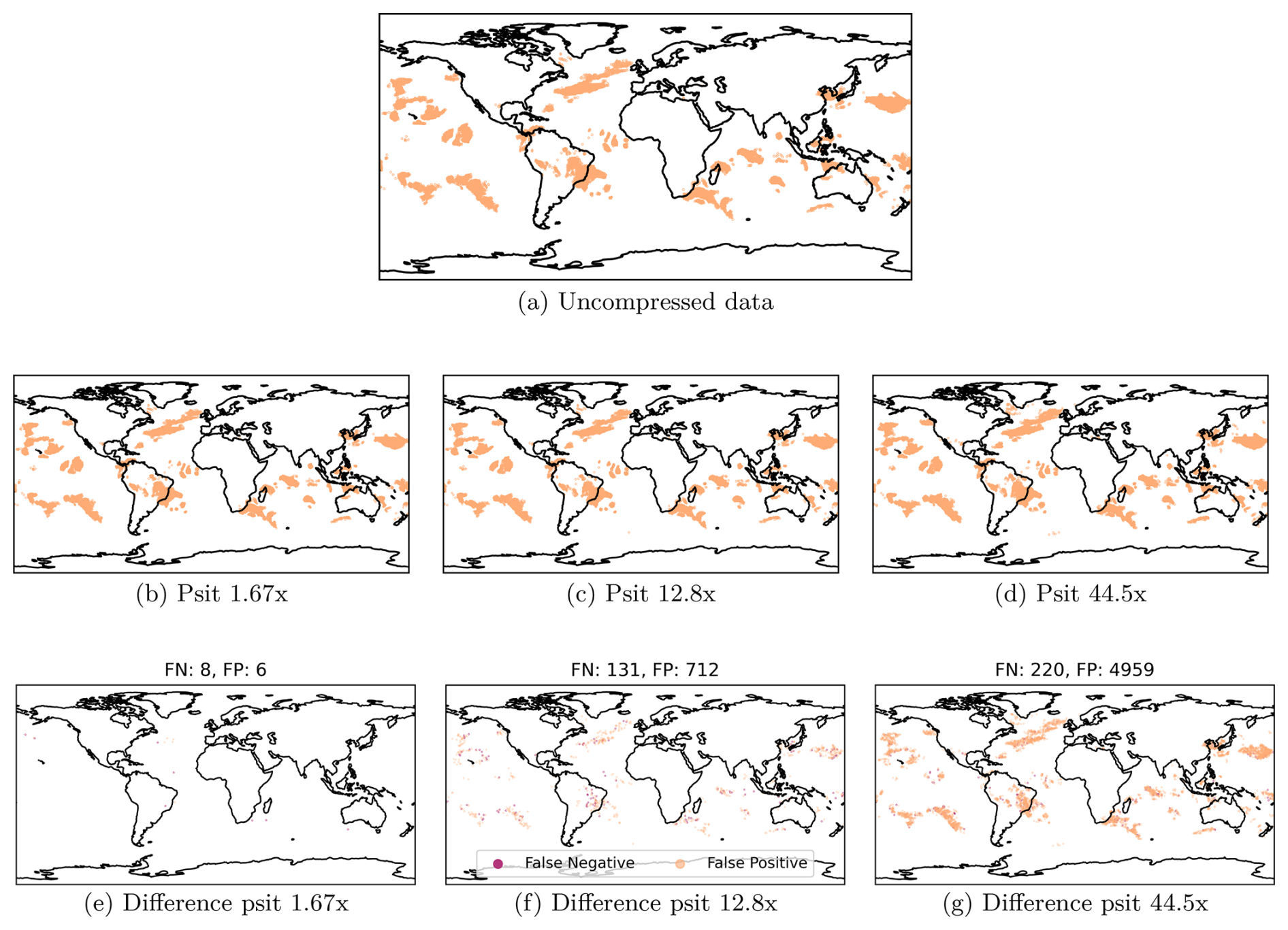
Figure 11 Warm Conveyor Belt calculations on the uncompressed data and the data compressed with psit at different compression ratios. Each point in a plot represents one trajectory which is part of a Warm Conveyor Belt (rises by at least 600 hPa in the first 48 h). Additionally the difference in term of false positive and false negatives is shown.

3.4.2 The Fukushima accident

During the Fukushima Daiichi accident (IAEA, 2015) in 2011, radiation-contaminated material was released into the atmosphere. This leads to the question of where this radioactive material is transported and deposited (Wotawa, 2011; Chino et al., 2011; Katata et al., 2012; Yasunari et al., 2011; Stohl et al., 2012). In this experiment, we want to discuss the impact compression has on trajectories originating in the region of the Fukushima Daiichi power plant. We will not perform any detailed deposition analysis.

For this, we create 35^′280 trajectories starting on 12 March 2011 at 00:00 in the box 140.74 to 141.3° E and 37.19 to 37.63° N over the pressure range of 764 to 996 hPa. The only information stored on the trajectories is their position, leading to a 59 MB file. For compression with psit, we choose JPEG 2000 with XYZ color and delta encoding. Note that here we compress trajectories that originate in a local region instead of a global one. We then compress the trajectories using psit, ZFP, and SZ3 with compression ratios around 6.5, 14, and 27. These compression ratios have been chosen to showcase both cases where compression works and cases where compression breaks down. We then plot the trajectories over time, as shown in Fig. 12. From the panels, we can see that for psit, ZFP, and SZ3 with increasing compression ratio, the results appear to get smoothed out and compression artifacts start to appear. We can also see that for psit the compression appears to perform worse, especially compared to Sect. 3.3. This is because the resulting grids have much smaller dimensions (48×37 grid points), leading to less data per grid, which results in poorer performance of the dense data compression algorithms. If we compare psit to the other two compression methods we can see that for lower compression ratios they are very similar to one another and only at the larger compression ratios can we observe psit delivering better results. This is in line with previous observations. This demonstrates that while psit is able to preserve the general structure and regions that would be affected, it is best used in the high ratio compression of files where many trajectories are present.

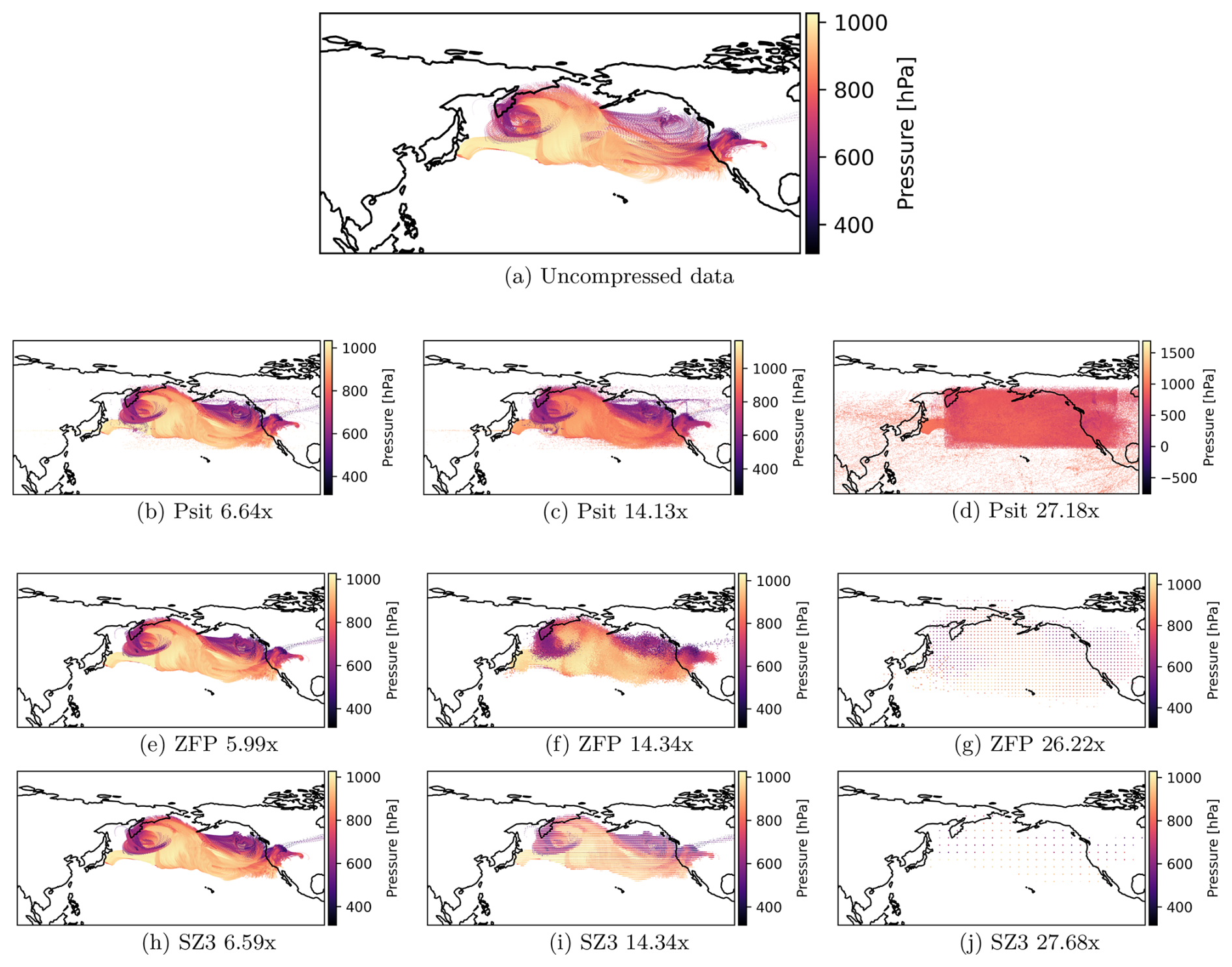
Figure 12 Comparison between trajectories starting at the site of the nuclear disaster at Fukushima for different compression ratios. On the top is the uncompressed data with, below it we have three rows of compressed data, one for psit, one for ZFP, and one for SZ3.

3.5 Throughput and Memory Usage

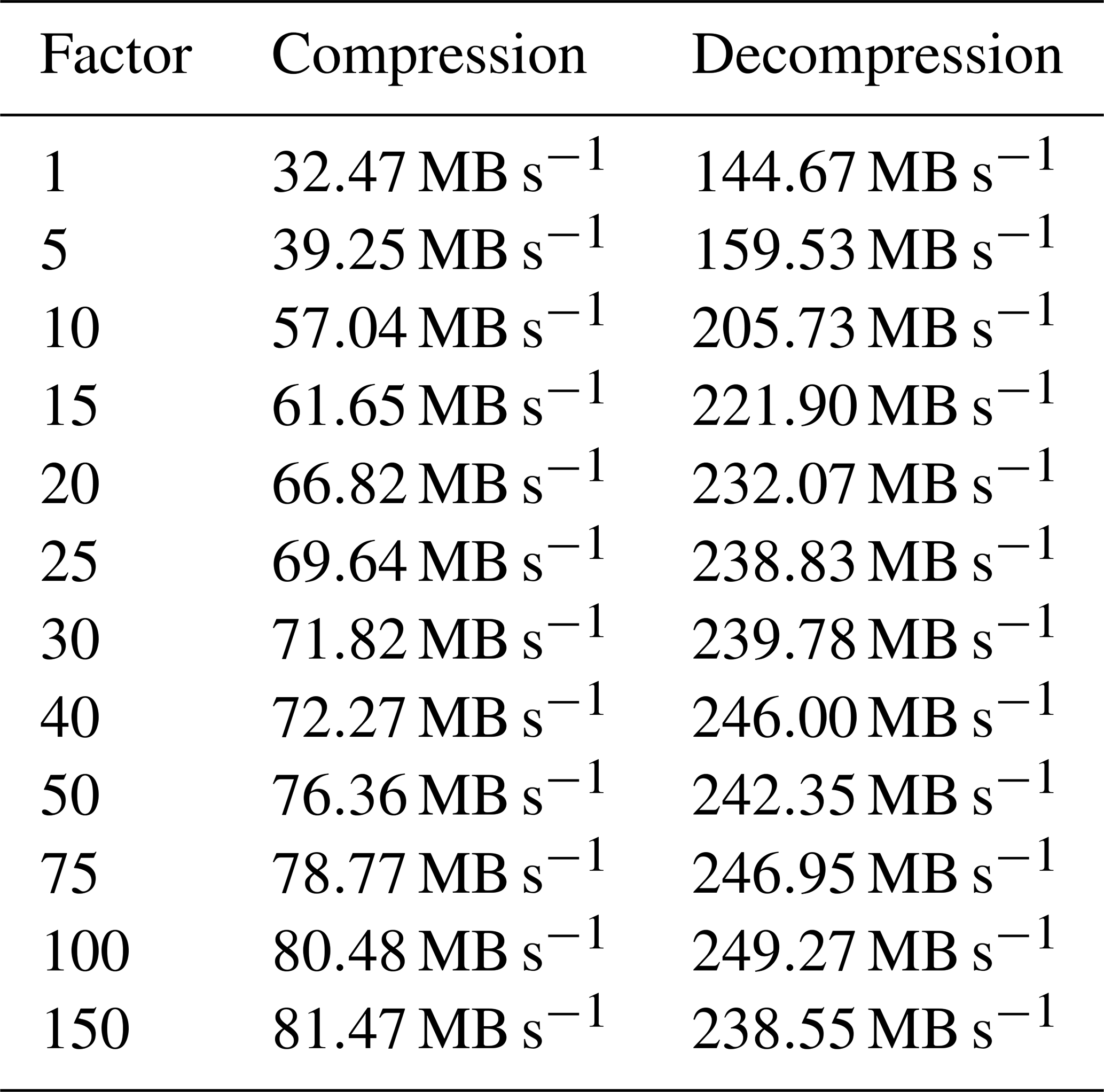
Until now, we have evaluated the performance of the program from an error standpoint. Here, we focus on performance from a computational perspective, discussing both throughput and memory usage. For this, the tra_20000101_00 trajectory file is compressed in the same manner as presented in Sect. 3.2. This is performed on an AMD EPYC 7742 parallelized over 37 threads (for both compression and decompression), using a ramdisk to filter out the impact of a slow filesystem. We then calculate the throughput in MB s⁻¹ for compression and decompression across the different compression ratios.

The results of the throuput experiments are presented in Table 4. The mean throughput of the compression stage is 65.67 MB s⁻¹, while the mean throughput of decompression is 222.14 MB s⁻¹. Decompression has a significantly larger throughput compared to compression because the expensive mapping stage only needs to be performed during compression. Another observation is that throughput increases as the compression factor gets larger. This is because a larger compression factor results in smaller file sizes, which, in turn, reduces the time needed to read and write data to disk. The memory usage for compression with factor 30 was 60 GB. The part where most of the memory consumption comes from is in solving the minimal weight full bipartite matching, which is parallelized over multiple workers. Therefore, one can trade memory usage against runtime by decreasing the number of parallel workers.

Table 4 Throughput for compression and decompression when running psit parallelized over 37 workers using a ramdisk.

4 Discussion

4.1 Applicable range and limitations

The main structural limitation of the program is the fact that the input data trajectories need to be uniformly distributed. This limitation originates from the way the mapping procedure has been implemented and has been touched upon in Sect. 2.5. The optimal fix for this limitation would be if the minimal weight full bipartite matching problem could be solved on a global level without having to restrict the grid points a trajectory may map to its closest 200 neighbors. A workaround for this is to artificially increase the ratio of grid points to trajectories, in this way, a mapping can be created at the cost of increased grid size, and because much of the data in the grids is redundant, the compression algorithms might be able to compress these grids more effectively, leading to only a small increase in output size.

In addition to the structural limitations, there are also performance limitations, especially memory consumption and runtime. Here, the bottleneck is the solving of the minimal weight full bipartite matching problem in the mapping phase. The only way to solve this would be to either use a different mapping method or find a more efficient implementation of such an algorithm. Additionally, all the images are currently saved individually, leading to the creation of potentially thousands of files, which can be slow on certain filesystems. Furthermore, currently the compression pipeline is written in Python and was developed parallel to the exploration of methods, leading to sometimes non optimal implementations.

Based on the above discussed limitations of the implementation, we argue that the applicable range of psit is in the compression of uniformly distributed trajectories in an HPC environment.

4.2 Future Work

Of course, one obvious area of future work would be fixing the current limitations of psit. This would include removing the limitation of a trajectory only being able to map to a set of its closest neighboring grid points and generally improving the overall computational performance of the pipeline in terms of runtime and memory usage. Fixing these limitations would be quite beneficial for psit, as it would allow it to be used in a wider range of applications.

The mapping method currently used by psit is based on graph theory, specifically the solution to a bipartite matching problem. However, there are likely other methods by which this could be done. For instance, instead of solving the problem directly in one step, an initial simple mapping (such as via nearest neighbors) could be created, which is then iteratively refined to fulfill the initial constraints, with the goal being to create a valid mapping that is also smooth. Further exploration of what “smooth” means could also be valuable. Currently, smoothness is achieved by using the trajectory positions at the first time step. What would happen if the mean position were used instead? Alternatively, could the smoothness of a grid be quantized to create a mapping that aims to optimize it? As the mapping phase is integral to the entire pipeline and currently presents the performance bottleneck, exploring these questions would be greatly beneficial.

The methods we use to describe compression performance are error metrics, comparison with perturbed/bitrounded wind fields, and real world examples in the form of two case studies. However, there are some intricacies to consider. Error metrics provide a straightforward way to quantify the incurred error, but they often lack a strong connection to real-world applications. It can be challenging to predict the impact of compression on real-world research based solely on a simple error metric. Is an RMSE error of 0.5 hPa in pressure acceptable, or should it be less than 0.3 hPa? Moreover, simple error metrics do not illustrate the relationship between different variables. How does the error in the longitude variable compare to the error in the latitude variable? Are they similar, or is there more error in one than the other? Does the error in the temperature variable depend on the pressure variable? A statistical analysis could examine correlations between various data variables, but this can quickly become tedious while leaving the fundamental question unanswered of how much correlation is acceptable. On the other hand, case studies simulate scenarios where the data might be used. We believe this approach establishes a better foundation for understanding the impact of compression. However, the challenge is that one can only analyze singular examples, and the generalizability of findings from one test to another remains an open question. While writing this paper, we spent considerable time discussing with experts in the field how such errors could be described and interpreted, there we found three major points that we think are important: compression should not change the outcome of experiments, compression errors should be smaller than measurement errors, compression should not influence the timings and occurrence of physical processes (e.g., cloud formation). But even these three points are not universally applicable, e.g., how does one compare measurement errors to compression errors, which physical processes are important enough to be conserved and to which degree should they be conserved. We tried to address these challenges in this paper, but we think that it would be beneficial and interesting to dedicate time into researching the possibilities of developing a benchmark that can help in understanding the impact of these errors. This benchmark could combine error metrics with a list of real-world applications, providing users with a general overview of how compression performs across different aspects.

5 Conclusions

The initial problem we faced and aimed to solve was that increasing computational power leads to an increase in data, making storage unfeasible. Therefore, a method needs to be devised to reduce it, with one approach being compression. While compression schemes exist for the Eulerian frame, no equivalent alternatives exist for the Lagrangian one. We therefore developed psit, a system to compress Lagrangian flows, to address this issue. In this paper, we presented how psit works and evaluated its performance using error metrics and case studies. In these, we demonstrated that in most cases, compression performance equivalent to or superior to ZFP and SZ3 can be achieved. We showed that the trajectory density of compressed trajectories (ratio 30 to 40) after 168 h behaves similarly to uncompressed trajectories calculated from perturbed wind fields (with a perturbation magnitude of $\mathrm{0.1}\mathrm{m}{\mathrm{s}}^{-\mathrm{1}}/\mathrm{6.67}\times {\mathrm{10}}^{-\mathrm{3}}$ Pa s⁻¹). Additionally, we analyzed the impact of compression on subsequent research through two case studies: warm conveyor belts and fallout prediction of the Fukushima accident. While psit imposes some limitations on the input data, namely requiring a uniform initial distribution, it can be used for general purpose compression of Lagrangian weather data and can serve as a foundation for further research in this area.

Appendix A: Proof of Total Unimodularity

In this section, we provide a proof that the LP presented in the LP mapping of Sect. 2.2 is an integral LP. An LP of the form $\mathit{\{}min{\mathit{c}}^T\mathit{x}|\mathbf{A}\mathit{x}\ge \mathit{b},\mathit{x}\ge \mathbf{0}\mathit{\}}$ is integral if the constraint matrix A is totally unimodular and the right hand side vector b is integral. In this mapping, the b vector consists solely of values equal to 1, making it integral. The only remaining step is to show that the matrix A is totally unimodular.

Before we begin the proof, we must discuss the structure of the matrix A. In the definition of the LP, it was stated that the vector x consists of the values x_t,p with t∈T and p∈P, and that there are two types of constraints:

$$\begin{array}{}\text{(A1)}& {\displaystyle }\sum _{t\in N^{-}\left(p\right)}{x}_{t,p}=\mathrm{1}\forall p\in P\text{(A2)}& {\displaystyle }\sum _{p\in N^{+}\left(t\right)}{x}_{t,p}\ge \mathrm{1}\forall t\in T\end{array}$$

Note that in contrast to the definition given in Sect. 2.2, here we also have the terms N⁻(p) and N⁺(t) which denote the possible matchings of trajectories to grid points, i.e., N⁻(p) for all the trajectories which may map to a point p and N⁺(t) for all the grid points which can be mapped by a trajectory t. This is such that the proof is also valid for the shortcuts we took during implementation. To transform these constraints into canonical form, we need to rewrite the equality constraint as a set of two inequalities. The relationship a=b can be expressed as a≥b and $-a\ge -b$. Thus, the constraints become:

$$\begin{array}{}\text{(A3)}& {\displaystyle }\sum _{t\in N^{-}\left(p\right)}{x}_{t,p}\ge \mathrm{1}\forall p\in P\text{(A4)}& {\displaystyle }\sum _{t\in N^{-}\left(p\right)}-x_{t,p}\ge -\mathrm{1}\forall p\in P\text{(A5)}& {\displaystyle }\sum _{p\in N^{+}\left(t\right)}{x}_{t,p}\ge \mathrm{1}\forall t\in T\end{array}$$

Next, we need to express these constraints in matrix form. To do this, we must establish a representation for the vector x. Without loss of generality, we can assume that x is constructed by first looping over all trajectories and then looping over all grid points to which each trajectory may map. This means that blocks of x_t,p with the same t and varying p are stacked on top of each other. For example, if we have three trajectories $t_{\mathrm{1}},t_{\mathrm{2}},t_{\mathrm{3}}$ and four grid points $p_{\mathrm{1}},p_{\mathrm{2}},p_{\mathrm{3}},p_{\mathrm{4}}$, the resulting vector x could look like this:

$$\begin{array}{}\text{(A6)}& \mathit{x}=\left[\begin{array}{c}{x}_{t_{\mathrm{1}},p_{\mathrm{2}}}\\ x_{t_{\mathrm{1}},p_{\mathrm{3}}}\\ x_{t_{\mathrm{2}},p_{\mathrm{1}}}\\ x_{t_{\mathrm{2}},p_{\mathrm{3}}}\\ x_{t_{\mathrm{3}},p_{\mathrm{4}}}\end{array}\right]\end{array}$$

With the shape of the vector x established, we can now construct the matrix A. This matrix consists of two parts. In the first part, called A₁, we encode the first two constraints (Eqs. A3 and A4), and in the second part, called A₂, we encode constraint Eq. (A5).

For the matrix A₁, each row corresponds to a grid point. A row resulting from constraint Eq. (A3) consists of 1s and 0s, with at most one 1 per block of the same trajectory in x. The exact distribution of these 1s depends on the shape of x, but what is important is that no two rows have a 1 in the same column. This follows directly from the structure of x and the fact that each row corresponds to a grid point. Another important property is that when constraints Eqs. (A3) and (A4) are combined, there are always pairs of rows that are identical, except that the sign of one row is the opposite of the other. Using the same example as above, the matrix A₁ will look like this:

$$\begin{array}{}\text{(A7)}& {\mathbf{A}}_{\mathrm{1}}=\left[\begin{array}{ccccc}\mathrm{0}& \mathrm{0}& \mathrm{1}& \mathrm{0}& \mathrm{0}\\ \mathrm{0}& \mathrm{0}& -\mathrm{1}& \mathrm{0}& \mathrm{0}\\ \mathrm{1}& \mathrm{0}& \mathrm{0}& \mathrm{0}& \mathrm{0}\\ -\mathrm{1}& \mathrm{0}& \mathrm{0}& \mathrm{0}& \mathrm{0}\\ \mathrm{0}& \mathrm{1}& \mathrm{0}& \mathrm{1}& \mathrm{0}\\ \mathrm{0}& -\mathrm{1}& \mathrm{0}& -\mathrm{1}& \mathrm{0}\\ \mathrm{0}& \mathrm{0}& \mathrm{0}& \mathrm{0}& \mathrm{1}\\ \mathrm{0}& \mathrm{0}& \mathrm{0}& \mathrm{0}& -\mathrm{1}\end{array}\right]\end{array}$$

Here, the pairs of rows with opposite signs are clearly visible.

Matrix A₂ results from constraint Eq. (A5). In this case, each row corresponds to a trajectory, and all columns are set to 1 where a corresponding x_t,p variable exists for that specific trajectory. Due to the construction of the x vector, all the different trajectories are grouped into blocks, and for each block, all the grid points that the trajectory can map to are indicated. Consequently, each row will contain a continuous sequence of 1s corresponding to the x_t,p values of the x vector with a specific t. This matrix will have a staircase structure, ensuring that no two rows have a 1 in the same column. Combining the previous part of A with this new one, it can be defined as follows:

$$\begin{array}{}\text{(A8)}& \mathbf{A}=\left[\begin{array}{c}{\mathbf{A}}_{\mathrm{1}}\\ {\mathbf{A}}_{\mathrm{2}}\end{array}\right]=\left[\begin{array}{ccccc}\mathrm{0}& \mathrm{0}& \mathrm{1}& \mathrm{0}& \mathrm{0}\\ \mathrm{0}& \mathrm{0}& -\mathrm{1}& \mathrm{0}& \mathrm{0}\\ \mathrm{1}& \mathrm{0}& \mathrm{0}& \mathrm{0}& \mathrm{0}\\ -\mathrm{1}& \mathrm{0}& \mathrm{0}& \mathrm{0}& \mathrm{0}\\ \mathrm{0}& \mathrm{1}& \mathrm{0}& \mathrm{1}& \mathrm{0}\\ \mathrm{0}& -\mathrm{1}& \mathrm{0}& -\mathrm{1}& \mathrm{0}\\ \mathrm{0}& \mathrm{0}& \mathrm{0}& \mathrm{0}& \mathrm{1}\\ \mathrm{0}& \mathrm{0}& \mathrm{0}& \mathrm{0}& -\mathrm{1}\\ \mathrm{1}& \mathrm{1}& \mathrm{0}& \mathrm{0}& \mathrm{0}\\ \mathrm{0}& \mathrm{0}& \mathrm{1}& \mathrm{1}& \mathrm{0}\\ \mathrm{0}& \mathrm{0}& \mathrm{0}& \mathrm{0}& \mathrm{1}\end{array}\right]\end{array}$$

The last step is to prove that this matrix is totally unimodular. The definition of total unimodularity states that for every square submatrix S of A, its determinant must be either −1, 0, or 1. Proving this directly can be quite challenging. However, Ghouila-Houri has shown that a matrix is totally unimodular if and only if for every subset R of rows of the matrix, there exists an assignment $s:R\to \pm$ of signs such that, when summed, every element in the resulting vector is either −1, 0, or 1. Therefore, we must find such a mapping $s:R\to \pm$ to conclude the proof.

To define this mapping, we use the property that in both parts of the matrix, no two rows have a 1 with the same sign in the same column. Initially, we assume that constraint Eq. (A4) does not exist, leading to the following definition of the mapping:

$$\begin{array}{}\text{(A9)}& \forall r\in R:s\left(r\right)=\left\{\begin{array}{ll}+& \text{if }r\in {\mathbf{A}}_{\mathrm{1}}\\ -& \text{if }r\in {\mathbf{A}}_{\mathrm{2}}\end{array}\right.\end{array}$$

We will first sum the vectors separately for the two parts, A₁ and A₂. Due to the previously mentioned property, the vector derived from A₁ will contain only elements from {0,1}, while the vector from A₂ will consist only of elements from $\mathit{\{}-\mathrm{1},\mathrm{0}\mathit{\}}$. The sum of these two vectors will thus produce a vector with elements from $\mathit{\{}-\mathrm{1},\mathrm{0},\mathrm{1}\mathit{\}}$, confirming that a valid mapping has been found.

Next, we will reintroduce constraint Eq. (A4) into the formulation. The mapping can be adjusted to accommodate this case by making a small extension: a row r∈R resulting from Eq. (A4) will be mapped to a − if and only if the same row with the opposite sign is not in R. In this way, two scenarios can occur: either both the positive and negative variants of a row are in R, in which case they will cancel out, or only one of them, either the negative or the positive variant, is in R. In the latter case, a − would be assigned to the negative variant, transforming the problem into the same form as if constraint Eq. (A4) did not exist at all. Therefore, it has been demonstrated that for any arbitrary subset R of rows from A, a mapping $s:R\to \pm$ has been found that makes the matrix totally unimodular, thereby proving that the LP is integral.

Appendix B: Additional performance data of psit

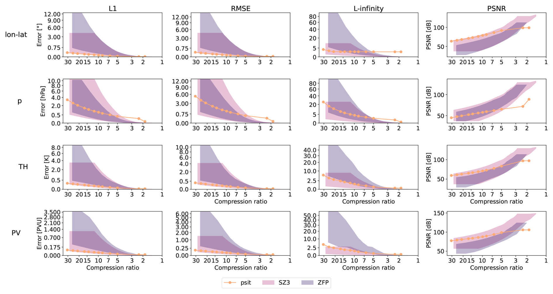
Figure B1 Comparison between psit, ZFP, and SZ3 for the tra_20200101_00 and tra_20200101_00_permuted files. The configuration of our program is described in Sect. 3.2 and the corresponding config file is given in Listing 1. The L1, RMSE, L-infinity error and PSNR is compared to the achieved compression ratio for the central angle error (lon–lat) and the other data variables (pressure (p), potential temperature (TH), and potential vorticity (PV)). In the plots the shaded area for ZFP and SZ3 corresponds to the range in compression performance between the two files. Note that psit performs the same for both, therefore, only one line is plotted.

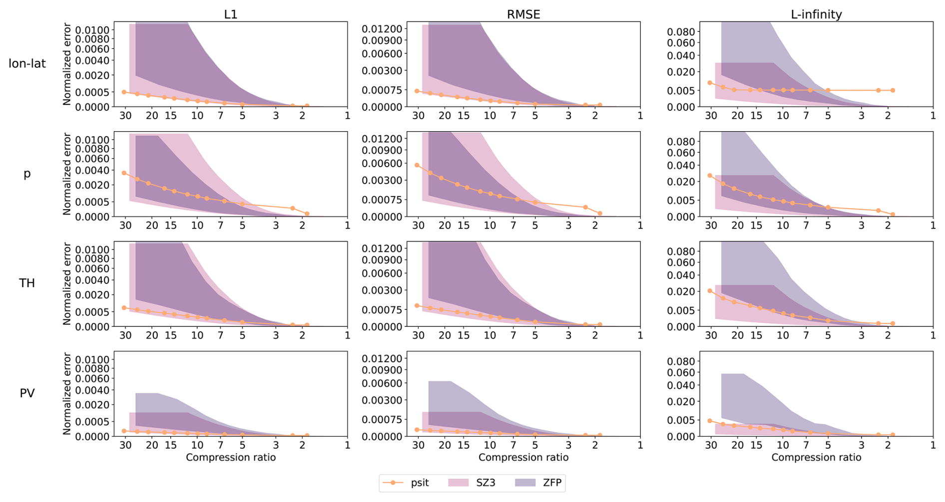
Figure B2 Data variable normalized error comparison between psit, ZFP, and SZ3 for the tra_20200101_00 and tra_20200101_00_permuted files. The configuration of our program is described in Sect. 3.2 and the corresponding config file is given in Listing 1. The L1, RMSE, and L-infinity errors are normalized and compared to the achieved compression ratio for the central angle error (lon–lat) and the other data variables (pressure (p), potential temperature (TH), and potential vorticity (PV)). In the plots the shaded area for ZFP and SZ3 corresponds to the range in compression performance between the two files. Note that psit performs the same for both, therefore, only one line is plotted.

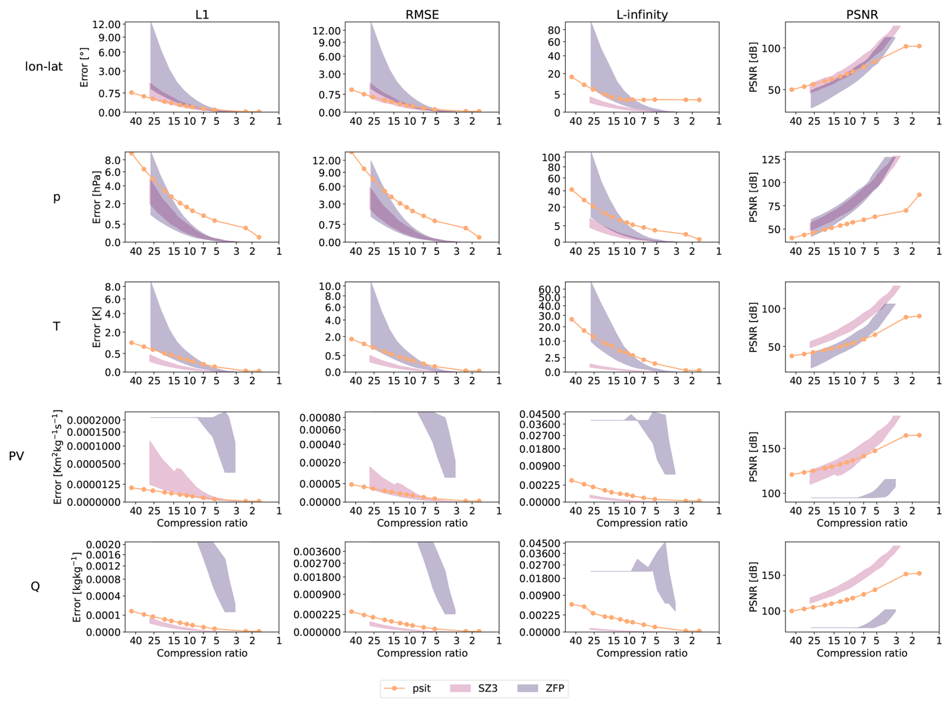
Figure B3 Comparison between psit, ZFP, and SZ3 for the tra_20000101_00 and tra_20000101_00_permuted files. The configuration of our program is described in Sect. 3.2 and the corresponding config file is given in Listing 1. The L1, RMSE and L-infinity error and PSNR is compared to the achieved compression ratio for the central angle error (lon–lat) and the other data variables (pressure (p), temperature (T), potential vorticity (PV), and specific humidity (Q)). In the plots the shaded area for ZFP and SZ3 corresponds to the range in compression performance between the two files. Note that psit performs the same for both, therefore, only one line is plotted.

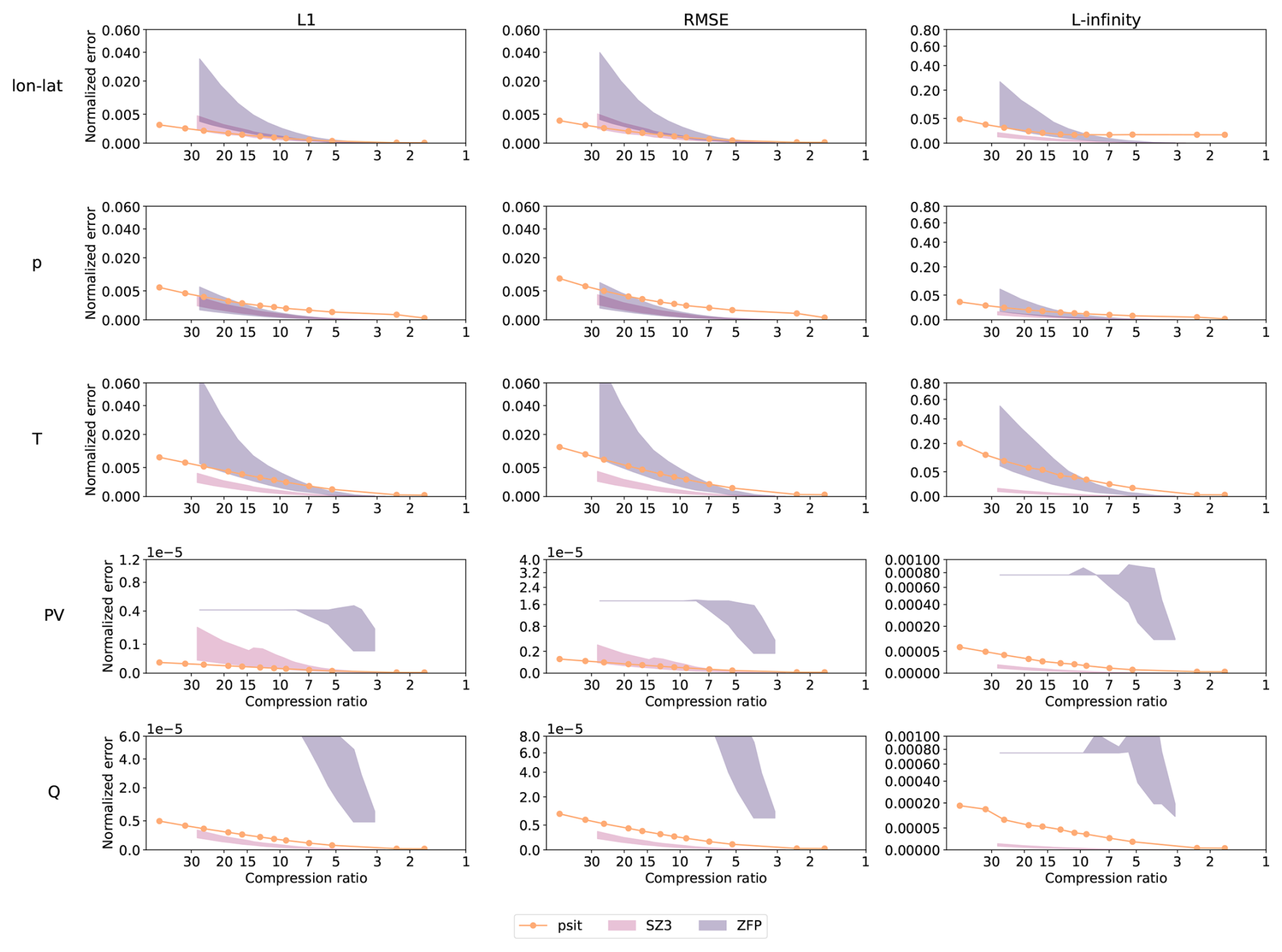
Figure B4 Data variable normalized error comparison between psit, ZFP, and SZ3 for the tra_20000101_00 and tra_20000101_00_permuted files. The configuration of our program is described in Sect. 3.2 and the corresponding config file is given in Listing 1. The L1, RMSE, and L-infinity errors are normalized and compared to the achieved compression ratio for the central angle error (lon–lat) and the other data variables (pressure (p), temperature (T), potential vorticity (PV), and specific humidity (Q)). In the plots the shaded area for ZFP and SZ3 corresponds to the range in compression performance between the two files. Note that psit performs the same for both, therefore, only one line is plotted.

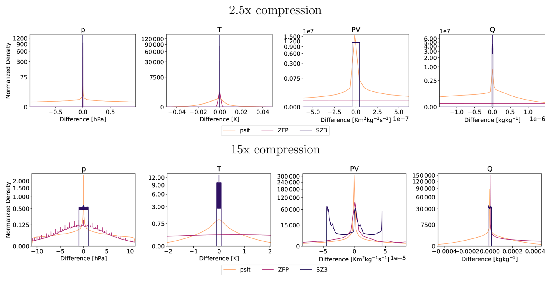
Figure B5 Area-normalized error distribution based on values for the tra_20000101_00_permuted dataset using the compression setup of Sect. 3.2 for psit with compression ratios of 2.5, and 15. The area of the densities have been normalized and the x axis is cropped to 2 standard deviations of the psit distribution for the 2.5 times compression case and 5 standard deviations for the 15 times compression case. The data variables are pressure (p), temperature (T), potential vorticity (PV), and specific humidity (Q).

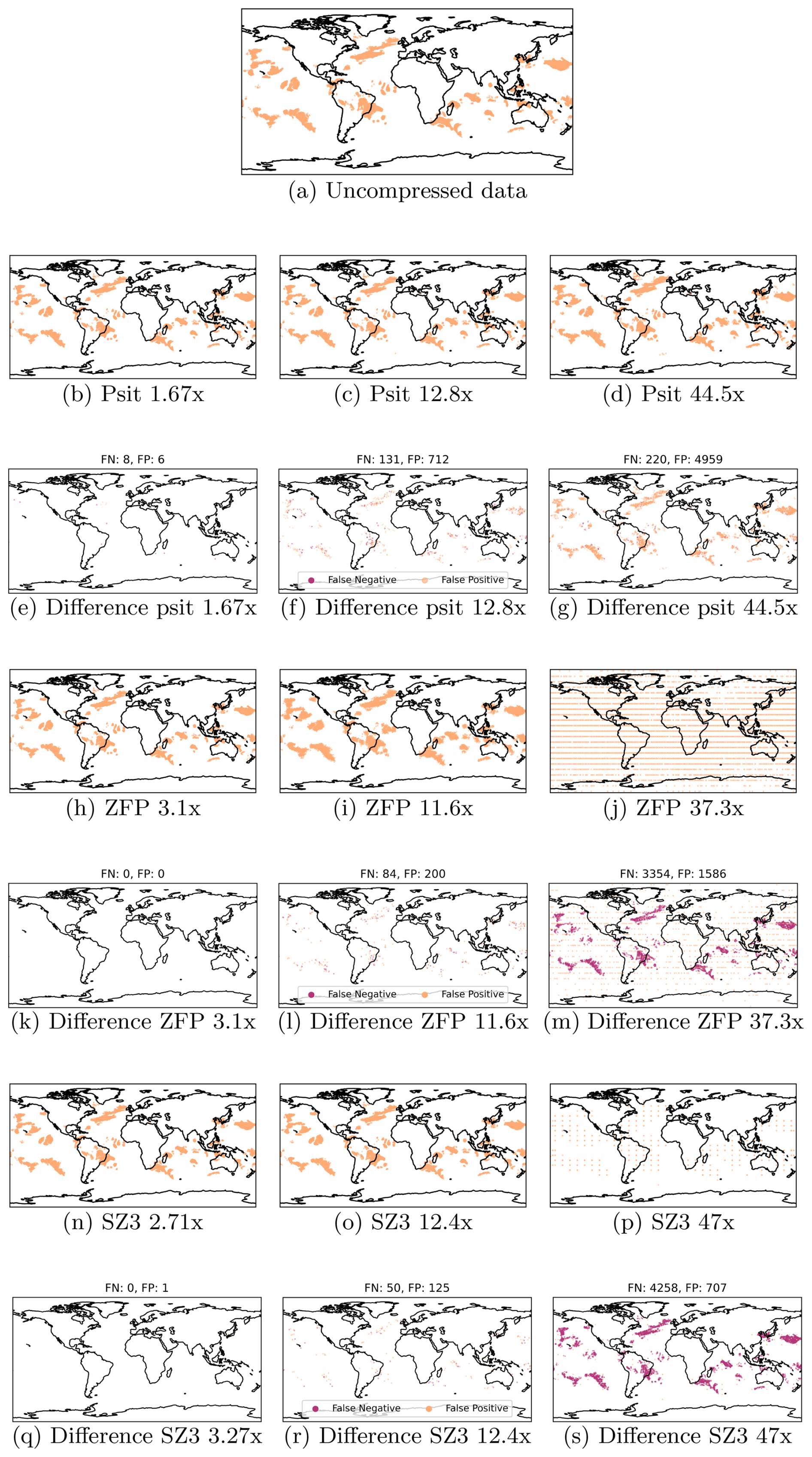
Figure B6 Warm Conveyor Belt calculations on the uncompressed data and the data compressed with different compression ratios and compressors. Each point in a plot represents one trajectory which is part of a Warm Conveyor Belt (rises by at least 600 hPa in the first 48 h). Additionally the difference in term of false positive and false negatives is shown.

Table B1 Error values and compression ratios for psit on the tra_20200101_00 dataset.

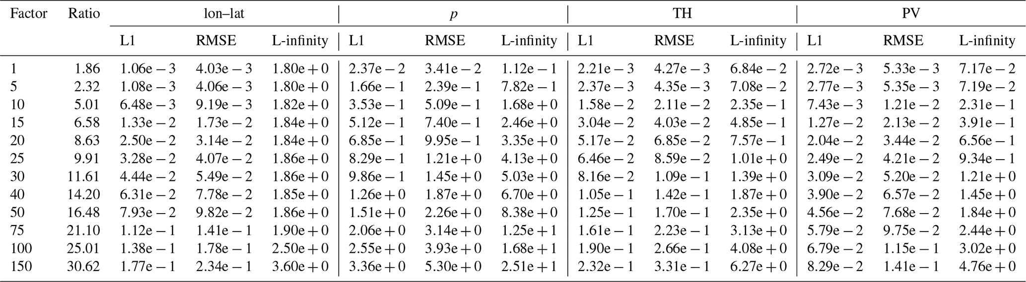
Table B2 Error values and compression ratios of the ZFP baseline run on the tra_20200101_00 dataset. Note that for some different tolerances the compression ratios are the same, this is probably because of the grouping into “bit planes” that is done by the embedded coding strategy of ZFP.

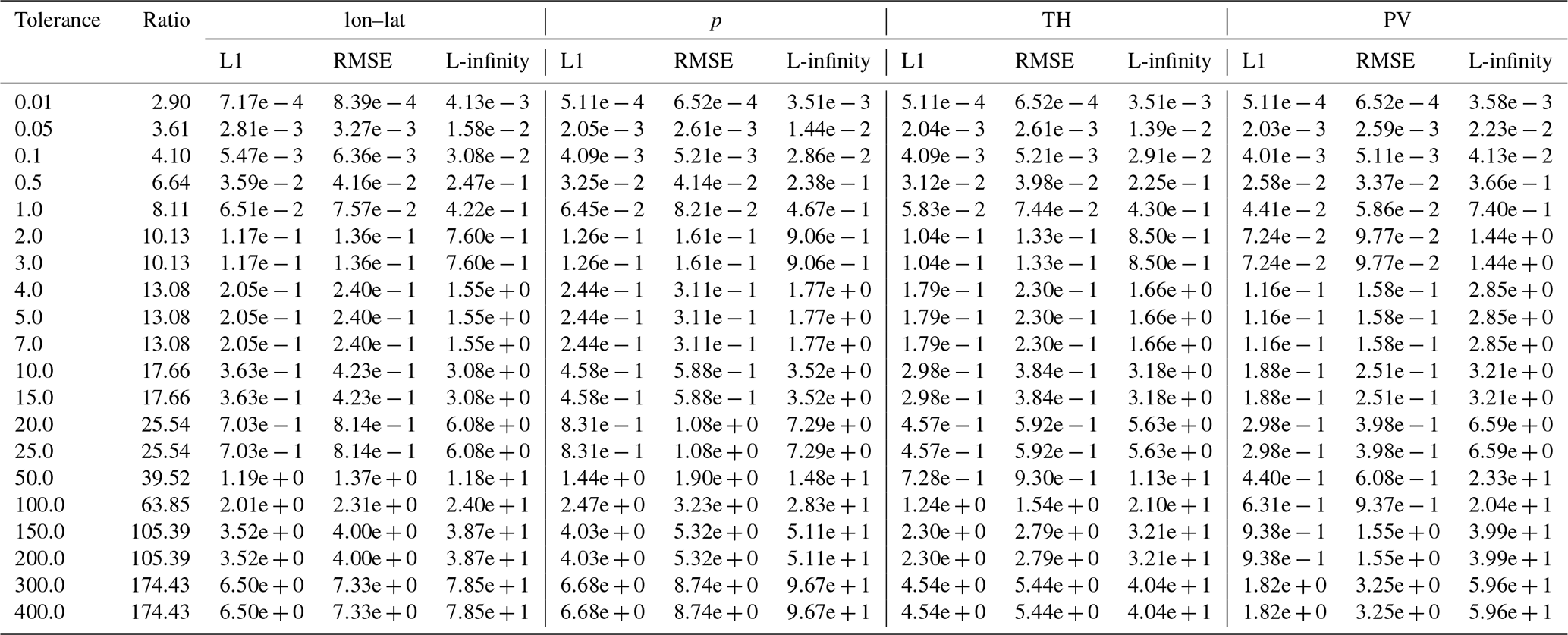
Table B3 Error values and compression ratios of the ZFP baseline run on the tra_20200101_00_permuted dataset. Note that for some different tolerances the compression ratios are the same, this is probably because of the grouping into “bit planes” that is done by the embedded coding strategy of ZFP.

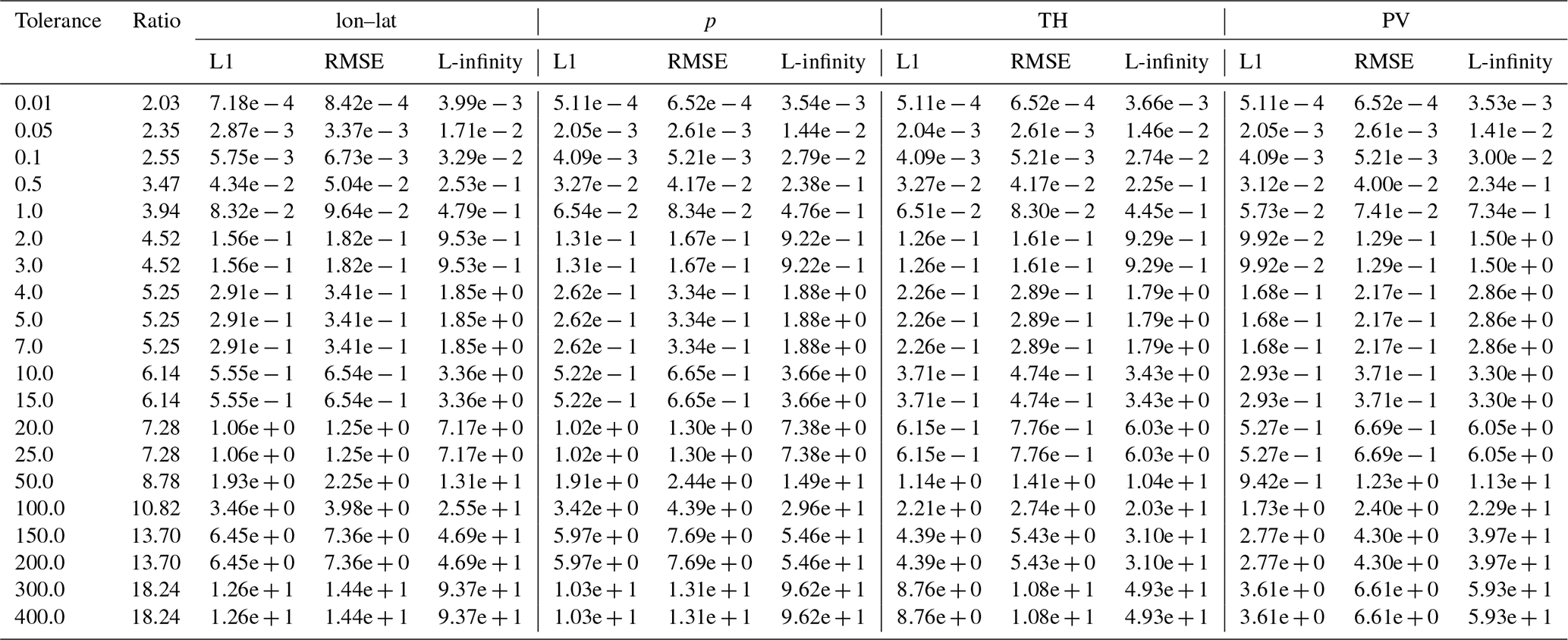
Table B4 Error values and compression ratios of the SZ3 baseline run on the tra_20200101_00 dataset.

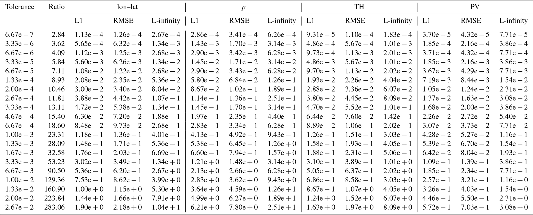
Table B5 Error values and compression ratios of the SZ3 baseline run on the tra_20200101_00_permuted dataset.

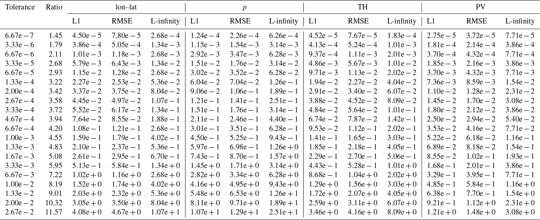
Table B6 Error values and compression ratios for psit on the tra_20000101_00 dataset.

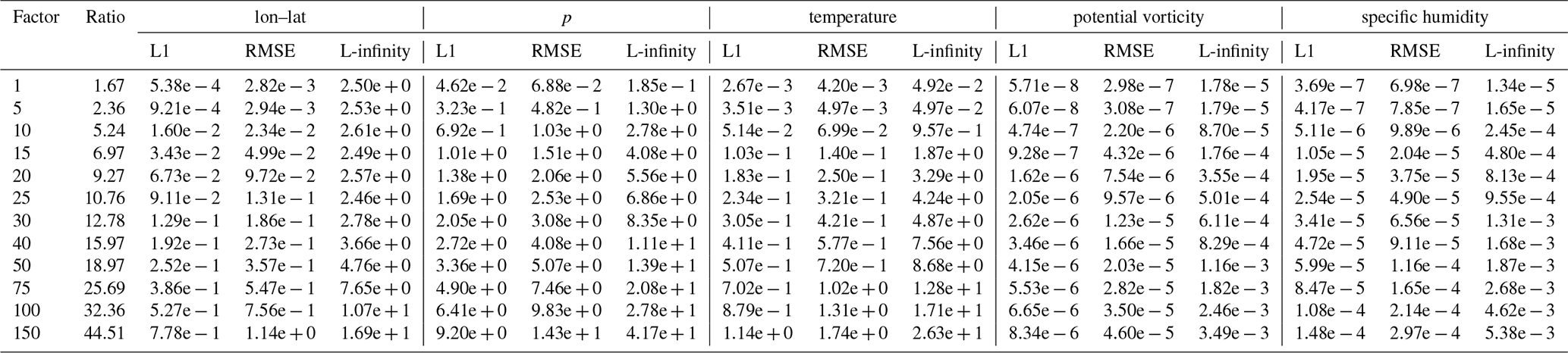
Table B7 Error values and compression ratios of the ZFP baseline run on the tra_20000101_00 dataset. Note that for some different tolerances the compression ratios are the same, this is probably because of the grouping into “bit planes” that is done by the embedded coding strategy of ZFP.

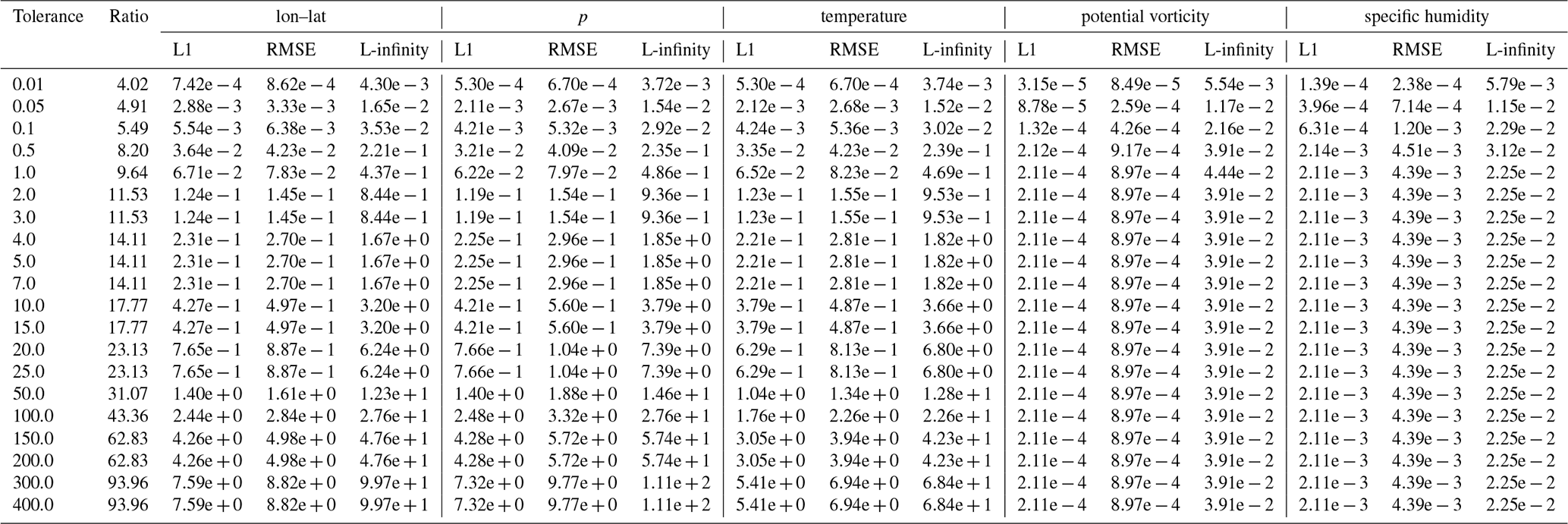
Table B8 Error values and compression ratios of the ZFP baseline run on the tra_20000101_00_permuted dataset. Note that for some different tolerances the compression ratios are the same, this is probably because of the grouping into “bit planes” that is done by the embedded coding strategy of ZFP.

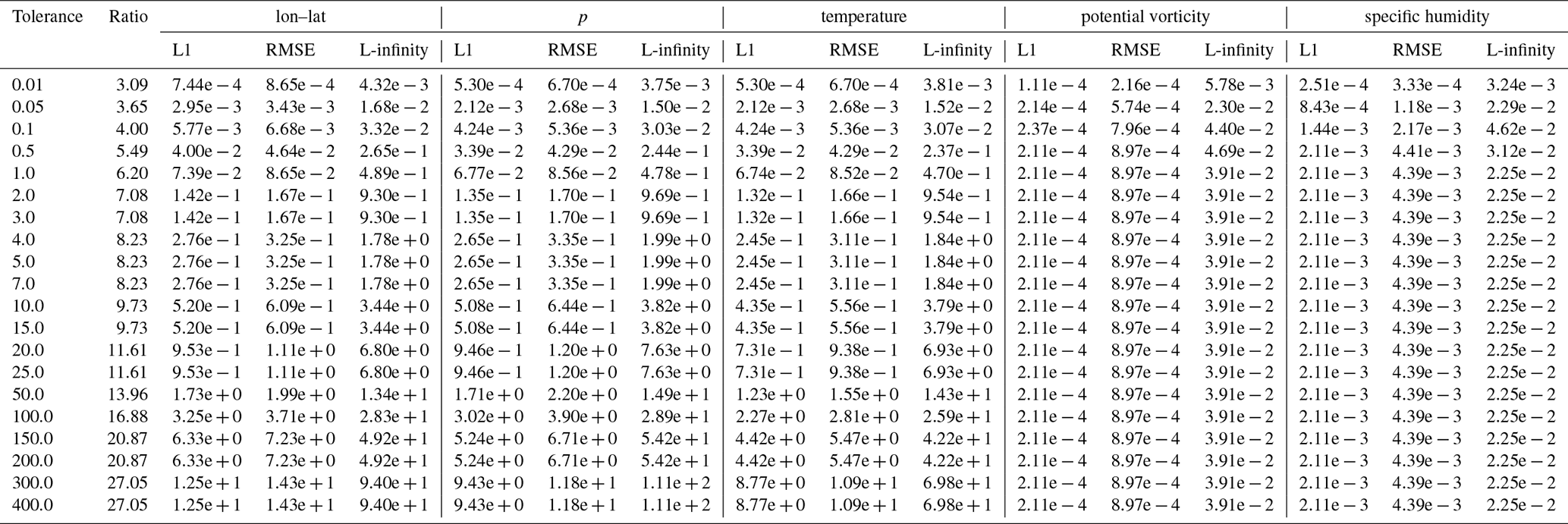
Table B9 Error values and compression ratios of the SZ3 baseline run on the tra_20000101_00 dataset.

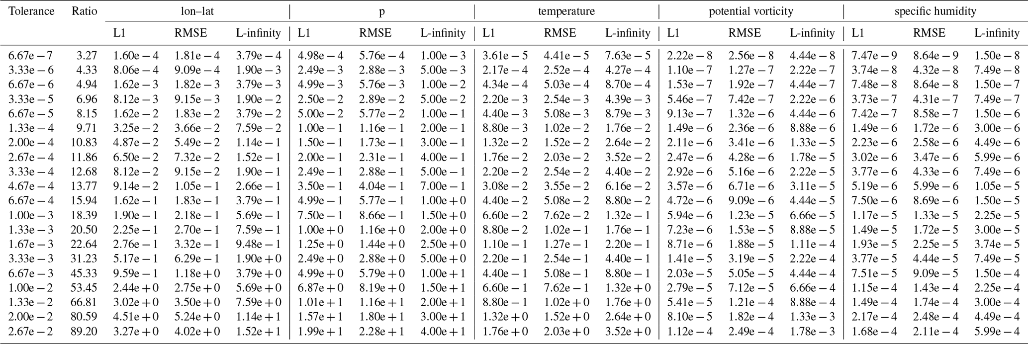
Table B10 Error values and compression ratios of the SZ3 baseline run on the tra_20000101_00_permuted dataset.

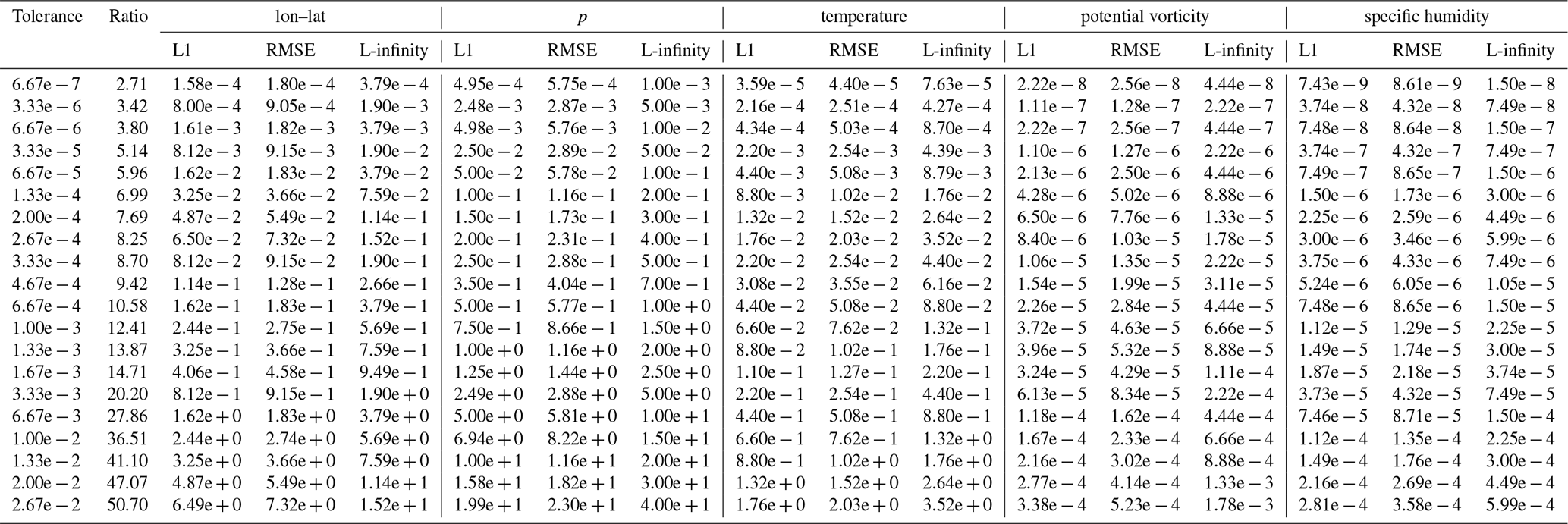
Table B11 Jensen–Shannon divergence metrics for different time steps for trajectories starting at 1 hPa.

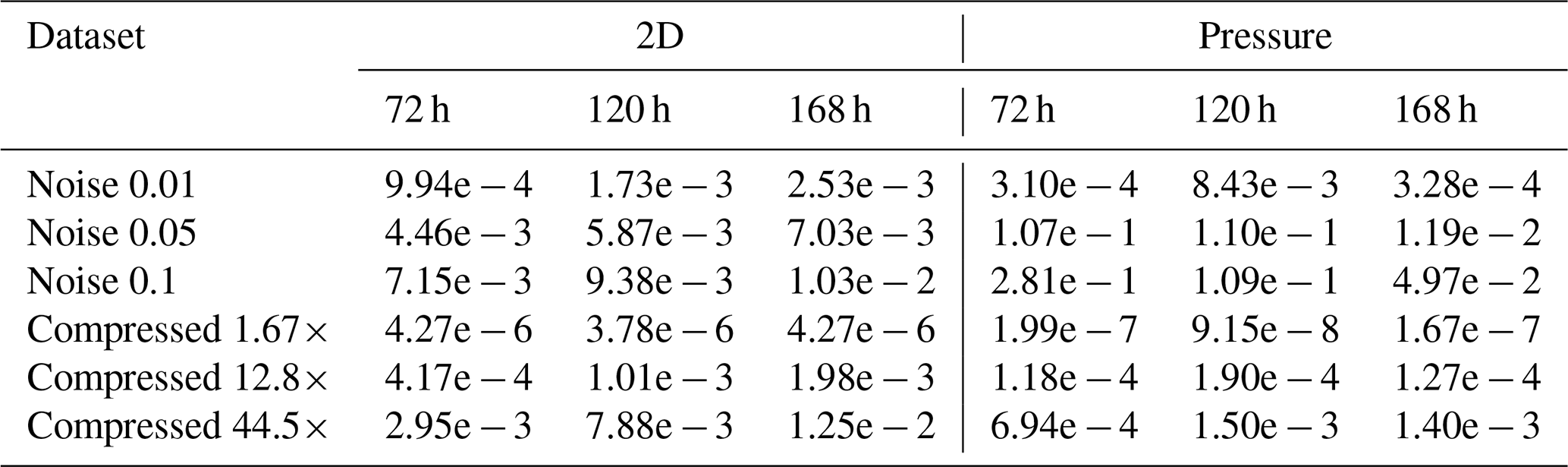
Table B12 Jensen–Shannon divergence metrics for different time steps for trajectories starting at 500 hPa.

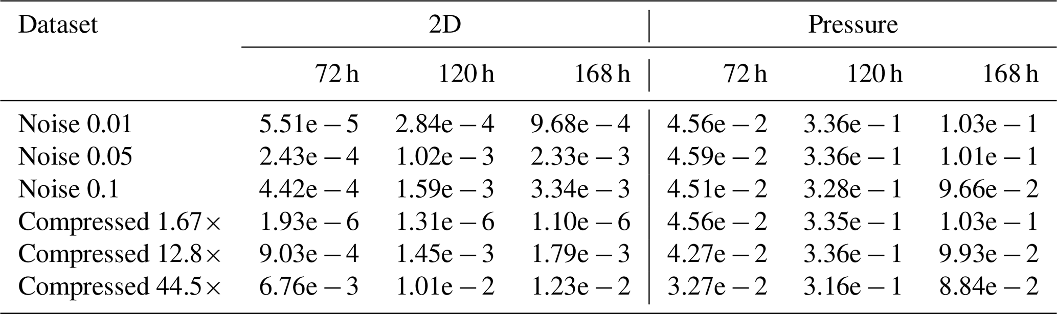
Table B13 Jensen–Shannon divergence metrics for different time steps for trajectories starting at 1000 hPa.

Appendix C: User Manual

In this section a small user manual for psit is given. For a detailed description please refer to (Pietak, 2025a). The psit compression pipeline has been implemented in Python, as this allowed for fast development and quick iteration of different ideas. The entire compression and decompression logic has been implemented in a class called Psit, which exposes two functions: compress() and decompress(). The compress() function takes an xarray.Dataset (with additional configuration parameters) as input and compresses it to a file on disk. The decompress() function takes the location of such a compressed file and returns an xarray.Dataset with the decompressed trajectory data. The additional configuration parameters, which can be passed to the compress() function, and a brief description are provided below.

• dataset. The xarray.Dataset we wish to compress.

• filename. The file in which the compressed data should be stored.

• crf. The compression factor.

• exclude. List of data variables which should not be compressed.

• method. The compression algorithm that should be used.

• color_method. The color encoding method that should be used.

• color_bits. The number of bits to use per color channel (when using color encoding).

• delta_method. The delta encoding method that should be used.

• local. If the trajectory starting positions are in a local domain and not global.

• bin] The number of pressure bins that should be used.

• mapping_func. Which mapping method should be used.

• num_workers. The number of parallel workers that should be used.

• factor. The ratio between number of grid points and trajectories.

• lon_name. Name of the longitude variable in the dataset.

• lat_name. Name of the latitude variable in the dataset.

• p_name. Name of the pressure variable in the dataset.

Note that some of these parameters, like crf or method, allow the individual setting of the parameter for each of the data variables available (using a dictionary mapping from variable name to value) in the dataset.

In addition to the Psit class, a CLI wrapper has been written called psitcli. This CLI wrapper allows for the easy compression of netCDF (Unidata, 2024) files from the command line. The program can be run with the command python psitcli.py {compress/decompress/test} [options] in_file out_file. The first option that needs to be defined is the mode to be used, this can either be compression, decompression, or test. The first two are used for compression and decompression, while the test mode will perform a compression followed by a decompression and the calculation of performance metrics such as the L1 error that was created. These additional metrics are stored as a Python pickle dump in a file called <out_file>_data.pick. The compress and test modes both take additional options, which mirror the ones accepted by the compress() function of the Psit class. Alternatively, these options can be defined via a YAML configuration file, which is then passed to psitcli. An example of such a configuration file is given in Listing 1.