Actionable reporting of CPU-GPU performance comparisons: insights from a CLUBB case study

Graphics Processing Units (GPUs) are becoming increasingly central to high-performance computing (HPC), but fair comparison with central processing units (CPUs) remains challenging, particularly for applications that can be subdivided into smaller workloads. Traditional metrics such as speedup ratios can overstate GPU advantages and obscure the conditions under which CPUs are competitive, as they depend strongly on workload choice. We introduce two peak-based performance metrics, the Peak Ratio Crossover (PRC) and the Peak-to-Peak Ratio (PPR), which provide clearer comparisons by accounting for the best achievable performance of each device. Using the performance of the Cloud Layers Unified by Binormals (CLUBB) standalone model as a case study, we demonstrate these metrics in practice, show how they can guide execution strategy, and examine how they shift under factors that affect workload. We further analyze how implementation choices and code structure influence these metrics, showing how they enable performance comparisons to be expressed in a concise and actionable way, while also helping identify which optimization efforts should be prioritized to meet different performance goals.

1 Introduction

High-performance computers increasingly employ Graphics Processing Units (GPUs), motivating efforts to use them to accelerate codes. However, porting large codebases to GPUs can require substantial development effort, making it important to have an expectation that the effort will be justified by performance gains. Many studies have compared the performance of GPU-accelerated implementations to traditional CPU implementations (Coleman and Feldman, 2013; Mielikainen et al., 2016; Wang et al., 2019, 2021; Shan et al., 2020; Watkins et al., 2022; Escobar et al., 2025; Jendersie et al., 2025), but it can be difficult to report the results in a way that allows the reader to clearly discern the conditions under which GPUs outperform CPUs.

CPUs and GPUs are architecturally distinct devices: CPUs prioritize low-latency execution in order to efficiently process small, quickly completed tasks, while GPUs trade latency for massive parallelism in order to efficiently process large tasks. As a result, device performance is highly sensitive to the workload – here defined as the volume of data processed within a single timestep. This usage is conceptually similar to the notion of a working set, but applied at the model-timestep scale: it reflects the total memory footprint actively touched across all variables, rather than just a cache-resident subset. Small workloads often favor CPUs, while large workloads favor GPUs. This workload sensitivity is evident in scaling studies in disparate domains, including atmospheric modeling components such as the Parameterization of Unified Microphysics Across Scales (PUMAS) (Sun et al., 2023) and the High-Order Methods Modeling Environment (HOMME) (Bertagna et al., 2019), as well as models in other domains (Kanur et al., 2015; Katsigiannis et al., 2015; Syberfeldt and Ekblom, 2017).

Because workload choice can dramatically change which device appears faster, performance comparisons depend strongly on whether the workload is fixed or can be varied. In some applications, workload is fixed to the problem size – the total volume of data to process – and cannot be easily changed. In others, such as general circulation models (GCMs), the problem can be subdivided into smaller workloads through batching techniques (Worley and Drake, 2005), allowing CPUs to be run at their most favorable workload instead of at a large, GPU-friendly workload.

Traditional performance metrics do not always capture this distinction. The commonly reported speedup – the ratio of GPU to CPU runtime at a chosen workload – is appropriate when workload is fixed to problem size, but for problems that allow computations to be flexibly batched, this direct speedup can be misleading. Such ratios may vary by orders of magnitude, allowing results to be reported only at scales that favor GPU execution. Similarly, the crossover point – the workload at which GPU performance surpasses CPU performance – is often used to guide device choice. Yet in problems that allow batching, CPU performance may be maximized at a workload different from the crossover, making the traditional crossover metric insufficient for determining which device is more performant.

To address these complexities, we introduce two metrics designed for problems that can be flexibly subdivided into batches. The first metric is a performance ratio, the Peak-to-Peak Ratio (PPR), defined as the ratio of each device's peak performance across all tested workloads. Because it compares each device at its own most favorable workload, PPR more fairly quantifies the speedup relevant to weak-scaling or ensemble use cases, where the problem size can grow to keep a device well filled with work and maximize sustained throughput. The second metric is a crossover metric, the Peak Ratio Crossover (PRC), defined as the workload at which GPU performance first exceeds the CPU peak. This makes PRC more useful for fixed-problem-size questions, as it more fairly determines which device is more performant, a common concern in strong-scaling scenarios where the goal is to minimize the runtime of a given problem by considering how best to subdivide it.

To demonstrate the utility of these metrics, we apply them to CLUBB standalone – a development version of the Cloud Layers Unified by Binormals (CLUBB) cloud and turbulence parameterization (Larson, 2022). Although typically configured as a single-column model (SCM), CLUBB standalone can execute ensembles (or batches) of grid columns in parallel. In this study, we define the batch size as the number of columns processed simultaneously, and measure throughput as the number of columns completed per unit time. Batch size does not fully determine the workload – workload also depends on factors like the number of vertical levels, numerical precision, and overall number of variables used – but batch size is a primary controllable parameter affecting it. By varying batch size, we explore a wide range of workload configurations, making CLUBB standalone a practical case study for evaluating our proposed performance metrics and comparing them with traditional ones.

We also investigate how performance is affected by implementation choices and code structure. These include choice of device, choice of directive method (i.e., OpenACC (Open Accelerators) vs. OpenMP (Open Multi-Processing)), use of asynchronous execution, and choice of numerical precision (single vs. double). Such implementation choices significantly influence measured performance, and they have different impacts on different metrics. Moreover, code structure itself can strongly affect relative performance: for example, in one of CLUBB's matrix-solving algorithms, simply reordering a few loops substantially alters CPU-GPU performance comparisons. This underscores the fact that performance differences often reflect not only hardware capabilities but also software optimizations that may favor one device over the other – a phenomenon that can skew comparisons (Lee et al., 2010).

The first half of this paper (Sects. 2–4) introduces our proposed performance metrics, explains their interpretation and application, and illustrates how different metrics are naturally better suited to different use cases depending on execution flexibility. Section 5 investigates how these metrics can be used to better describe the different performance impacts that different implementation choices have, and Sect. 6 investigates how well CLUBB is optimized on both CPU and GPU platforms and outlines key opportunities for future performance improvements.

2 CLUBB description

CLUBB (Cloud Layers Unified by Binormals) is a single-column parameterization of turbulence and clouds. CLUBB calculates the vertical transport of heat content, moisture, and momentum, and it diagnoses the fraction of a grid level occupied by cloud. To calculate these quantities, CLUBB approximates and solves differential equations in time and height by use of finite differences. CLUBB is used by default in both the Community Earth System Model (CESM) and Energy Exascale Earth System Model (E3SM) 2.0 (Larson, 2022; Danabasoglu et al., 2020; Golaz et al., 2022). Within these GCMs, CLUBB serves as one of the atmospheric physics components in CAM (Community Atmosphere Model), alongside other parameterizations such as RRTMGP (Rapid Radiative Transfer Model for Global Climate Models – Parallel) and PUMAS (Iacono et al., 2008; Bogenschutz et al., 2018; Gettelman et al., 2023).

In addition to its role in global atmospheric models, CLUBB is also maintained in a standalone model, primarily used for development and testing. CLUBB was originally designed to operate on a single atmospheric grid column (i.e., one set of vertical levels) per execution. However, as part of recent GPU porting efforts, CLUBB has been extended to support processing multiple columns simultaneously. Historically, the standalone version ran one case at a time, but it has now been upgraded to support ensemble-style runs where each column represents a different set of parameter values applied to the same base case. While the GPU port was originally motivated by CLUBB's use in host models, this new capability enables efficient use of HPC systems for large-scale parameter tuning.

The standalone version, being smaller and more modular than the full host models, serves as a convenient test bench for performance analysis. It allows experimentation across a wide range of configurations – including different directive methods, compilers, and hardware targets – while still mimicking the structure of a host model run, with multiple MPI (Message Passing Interface) tasks processing a fixed number of columns per task (Message Passing Interface Forum, 2024). This makes performance insights from the standalone model directly relevant to CLUBB's behavior in GCMs.

CLUBB is written in Fortran and comprises approximately 100 000 lines of code. GPU support was implemented using OpenACC, with 879 loop directives and 141 data directives. This approach enables a unified codebase that performs efficiently on both CPUs and GPUs. The full porting effort took roughly three years, with the most labor-intensive task being the restructuring of code to push the column loop downward into low-level regions. A similar restructuring process, applied to the separate PUMAS codebase rather than CLUBB, is described by Sun et al. (2023). Now that this restructuring is complete and the OpenACC code is functional, the codebase can be converted when needed to OpenMP target offloading directives using Intel's migration tool (Intel, 2024). CLUBB is also regularly compiled and tested across multiple compilers and build settings to ensure portability across platforms.

To enable concurrent processing of multiple columns in CLUBB, input and output variables were redefined as two-dimensional arrays, indexed by the number of columns (N_i) and vertical levels (N_z), or (ngrdcol,nz) in Fortran. This redimensioning effort, along with loop restructuring, resulted in a common code pattern across CLUBB: nested loops over columns and levels, often referred to as ik-loops, with the i-loop over columns innermost to promote vectorization and ensure contiguous memory access on CPUs. While a small number of loops include vertical dependencies – preventing vectorization or GPU loop collapsing and making them relatively more expensive – the vast majority are independent over both dimensions.

3 Timing methodology

To gather performance measurements from CLUBB standalone, we focused on the original continental shallow cumulus intercomparison case at the ARM (Atmospheric Radiation Measurement) Southern Great Plains site (Brown et al., 2002). In CLUBB standalone, this case is run with 134 vertical levels by default. To simulate multiple columns, we configure each run with a set of unique parameter sets, with each parameter set assigned to a separate column. Because a single CLUBB standalone instance runs in serial, we use mpirun (or srun) to launch multiple MPI tasks, each running a separate instance with the same number of columns per task. The overall batch size is therefore the number of MPI tasks multiplied by the number of columns per task, and the runtime we report corresponds to the wall-clock time of the full mpirun job – effectively the greatest runtime that any MPI task takes to complete a batched run. This setup both ensures effective hardware utilization and closely mirrors the execution model used when CLUBB is embedded in a GCM. However, absolute timing results may not extrapolate directly to host-model runs, because host models have a greater overall memory footprint and differ in the amount of non-CLUBB work performed by each MPI task.

The results we present measure only the time spent in the core time-stepping loop, which contains the useful computational work. To isolate this, we subtract the runtime of a zero-iteration baseline run from the total execution time. This eliminates startup costs such as namelist reading, memory allocation, and any initial CPU-GPU memory transfers. Disk output is also disabled in all runs. In most configurations, these startup costs are negligible relative to total runtime. For small problem sizes on the CPU, startup time can be a larger fraction, but still remains secondary. Expensive GPU memory transfers occur entirely outside the time-stepping loop and are thus excluded. The only memory transfers that contribute to the runtime cost we measure are the result of OpenACC (or OpenMP) reduction operations.

The ARM case simulates 870 timesteps with a 60 s timestep. To minimize noise in the timing numbers, all configurations are run for the full 870 timesteps, and the reported performance is that of the average cost per timestep. Repeated tests indicate good consistency between measurements: GPU runtimes vary by less than 2 %, and CPU runtimes by less than 5 %.

Table 1 lists the hardware and compiler configurations used for the reported results. Derecho (NSF NCAR, 2025b) and Casper (NSF NCAR, 2025a) are operated by NSF NCAR, while Frontier (ORNL, 2025) is operated by Oak Ridge National Laboratory (ORNL). CPU results were compiled with Intel ifx and GPU results with NVIDIA's nvfortran, except on Frontier, where Cray's crayftn was used for both CPU and GPU runs.

Table 1 Hardware and compiler configurations of the nodes used for reported results. All compilers were invoked with -O2 optimization and 256-bit vector instructions, and -Mstack_arrays was applied for nvhpc builds.

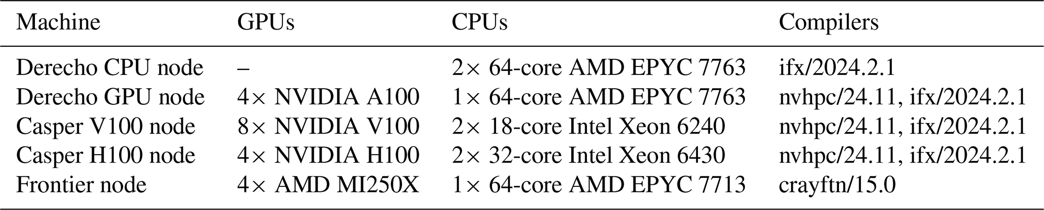
As a result of the large number of comparisons we make, there is little consistency between the number of devices or MPI tasks we profile with. GPU runs generally use one task per GPU, but the effect of oversubscription is discussed briefly in Sect. 5.5. For CPU runs, we assign one task per core, since further oversubscription did not improve performance and added variability. To make this clear in each comparison, each configuration is labeled using a “_MxN_” qualifier, where M is the number of physical devices (e.g., CPUs or GPUs) and N is the number of MPI tasks. For example, a result with “_2x128_” in its label represents a run with two devices and 128 MPI tasks, which can be seen in results using two 64-core CPUs.

4 GPU vs. CPU performance

Comparing CPU and GPU performance depends on how efficiency varies with workload. As discussed earlier, CPUs tend to perform best at small workloads, while GPUs improve as workloads grow. With any usage of CLUBB, the overall goal (or problem to solve) is to process a given number of columns, and because columns are independent we can freely choose the batch size without changing numerical results. This flexibility provides some freedom over the workload used, as we can solve the problem using many small batches or a few large ones. Raw runtimes across different batch sizes, however, are not directly comparable – larger batches naturally take longer – so we use a throughput-based view to compare efficiency of different batch sizes on equal footing.

4.1 Throughput metric

The metric we use to quantify performance is throughput: the number of columns CLUBB can advance by a timestep per unit wall-clock time. Throughput is defined as:

$$\begin{array}{}\text{(1)}& T\left(N_i\right)\equiv {\displaystyle \frac{N_i}{R\left(N_i\right)}},\end{array}$$

where N_i is the number of columns processed simultaneously (the batch size), and R(N_i) is the average runtime consumed by one of these CLUBB timesteps for one batch of size N_i, resulting in the throughput, T, having units of “columns per second”.

Analyzing throughput allows us to identify the batch size, N_i, that maximizes efficiency: the optimal N_i is the one that maximizes T(N_i). For a total of N columns to process using a batch size of N_i, the total runtime is given by $N/T\left(N_i\right)$, which is minimized when N_i maximizes throughput, T.

4.2 Performance metrics

When plotting CPU and GPU throughput as a function of batch size, four key performance metrics emerge naturally. They provide insight into different usage scenarios. Two of the metrics are crossover points – namely, the workloads at which GPU performance surpasses that of the CPU. The other two are performance ratios – they quantify the relative advantage of GPU execution at large problem sizes. Figure 1 illustrates these metrics by comparing CLUBB standalone performance on four NVIDIA A100 GPUs versus a dual-socket node with two 64-core AMD EPYC 7763 CPUs. This effectively compares a fully utilized “GPU node” against a fully utilized “CPU node”, corresponding to the two types of node found on Derecho.

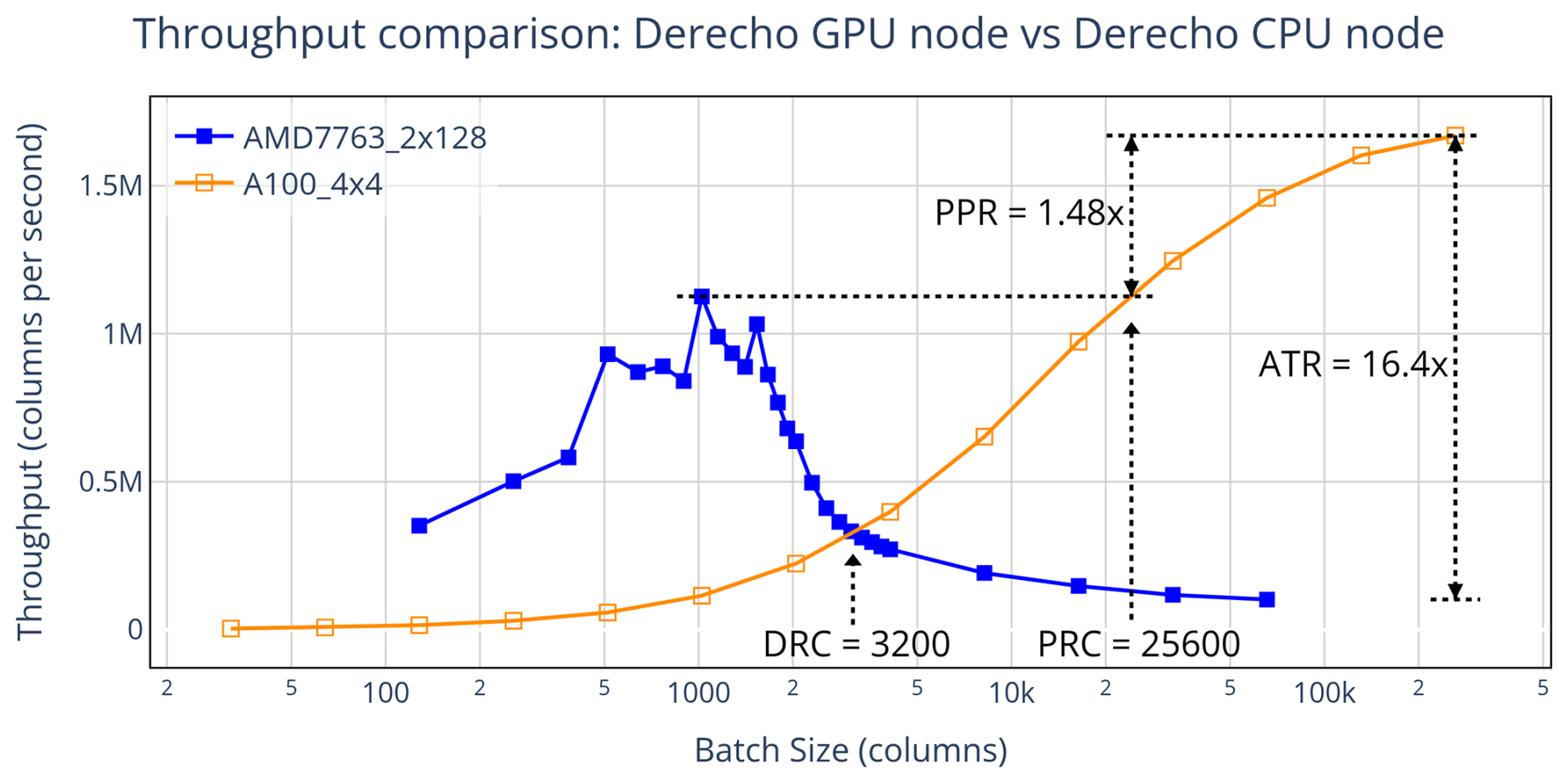
Figure 1 Throughput comparison between a Derecho GPU node (using four NVIDIA A100 GPUs) and a Derecho CPU node (using two 64-core AMD 7763 CPUs). Crossover metrics (PRC, DRC) guide device choice: PRC (Peak Ratio Crossover) identifies the batch size at which GPU throughput surpasses the best-case CPU throughput, while DRC (Direct Ratio Crossover) identifies the batch size at which GPU performance begins to exceed CPU performance directly. Performance-ratio metrics (PPR, ATR) quantify differences: PPR (Peak-to-Peak Ratio) compares peak throughput at each device's optimal batch size, and ATR (Asymptotic Throughput Ratio) is the large-workload ratio.

1. Crossover metrics

   Crossover metrics help us decide whether a run is better suited to CPUs or GPUs. The Peak Ratio Crossover (PRC) is defined as the smallest batch size at which GPU throughput exceeds the best throughput that the CPU achieves across all tested batch sizes. PRC is relevant for models in which batch size is freely tunable, such as CLUBB.

   In contrast, the Direct Ratio Crossover (DRC) becomes the relevant metric when the problem cannot be freely subdivided. For example, CLUBB includes vertical coupling, and so changing the number of vertical levels affects the workload but also alters the numerical results – meaning the number cannot be changed solely for performance reasons. If the goal were to study how performance scales with vertical resolution in single-column CLUBB runs, this would result in a similar investigation, but each configuration would represent a distinct physical problem, making cross-workload comparisons inappropriate. In such cases, the DRC – defined as the batch size at which GPU throughput overtakes CPU throughput when both are measured at the same batch size – serves as a suitable decision metric.

2. Performance ratio metrics

   The performance ratio metrics, by contrast, do not inform device selection for a specific problem size, but instead quantify the performance difference between CPUs and GPUs in the limit of large problem size. When flexible subdivision is possible, the relevant metric is the Peak-to-Peak Ratio (PPR): the ratio of maximum GPU throughput to maximum CPU throughput, each measured at its respective optimal workload. The PPR is the most informative measure of large-problem GPU performance advantage for codebases that support flexible batching, such as CLUBB.

   For a problem that cannot be flexibly batched, the Asymptotic Throughput Ratio (ATR) is a more relevant measure of the performance difference at scale. This metric compares raw throughput ratios at each batch size and identifies the ratio at the largest workload tested. Direct ratios like this can swing dramatically with workload, limiting their usefulness for characterizing performance across scales.

Figure 2 summarizes which performance metric is most applicable, based on batching flexibility and the specific performance question being asked. Another useful way to think about metric choice is through a scaling lens. The PRC is more valuable to someone analyzing a fixed-problem-size scenario in a strong-scaling analysis, where the total problem size is fixed but the number of cores, devices, or batch sizes used to subdivide the work can vary. In contrast, the PPR is more useful in a weak-scaling analysis, where the problem size can grow by adding additional copies of the same underlying workload component to keep the devices fully utilized.

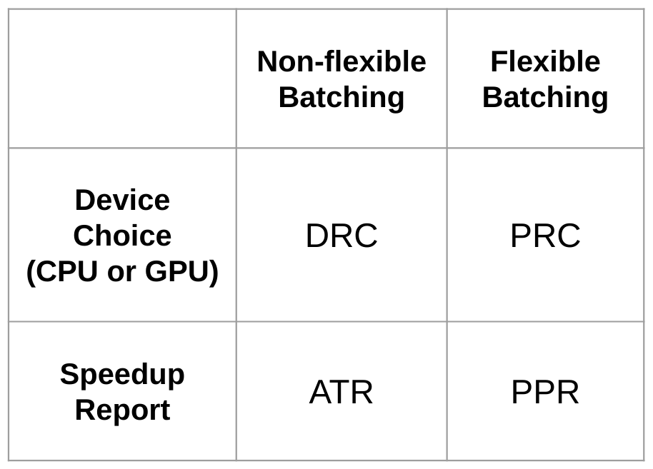
Figure 2 The most relevant metric depends on whether the problem can be divided into smaller workloads and on the specific question being asked. Device selection can be guided by the crossover metrics (DRC or PRC), while quantifying the speedup between devices is best done using the throughput ratio metrics (ATR or PPR).

From the comparison of CLUBB throughput in Fig. 1, we observe a Peak-to-Peak Ratio (PPR) of 1.48×, with the CPU node reaching peak throughput at a batch size of 1024 columns (8 columns per core across all cores) and the GPU node reaching its peak at the largest batch size that fits in memory: 262 144 columns in total (65 536 per GPU). In practical terms, if the problem is to run CLUBB standalone on a large number of columns, say N, the optimal strategy is as follows: on the CPU node, process batches of 1024 columns at a time, requiring $N/\mathrm{1024}$ batches; on the GPU node, process batches of 262 144 columns, requiring $N/\mathrm{262}\mathrm{144}$ batches. Under these strategies, the CPU node takes longer to complete the full task, approximately 1.48 times the runtime that it would take a GPU node.

The Peak Ratio Crossover (PRC) is 25 600 columns. This identifies the point at which the GPU becomes the faster choice for a given problem size. Using N as the total number of columns to process – if N≤25 600, the largest workload that fits on the GPU is too small for its throughput to exceed that of the CPU, making a CPU node the optimal choice (when using repeated, optimally batched runs). When N>25 600, a GPU node completes the task faster, even if the entire problem can be processed in a single batch smaller than the size required for the GPUs to reach peak throughput.

Because the problem of running CLUBB on many columns can be flexibly batched, the Direct Ratio Crossover (DRC) and Asymptotic Throughput Ratio (ATR) are less central to it. The ATR is 16.4×, which indicates a big advantage for GPUs if a run is done at the largest workload. In particular, the ATR is more than 11 times higher than the PPR. This illustrates how ATR could potentially be misused to overstate GPU advantage for problems that can be subdivided into smaller workloads. A similar overstatement is possible for the DRC (3200 columns), which is roughly 8 times smaller than the PRC. In contrast, for problems that cannot be flexibly batched, the DRC and ATR would be the more appropriate metrics to use.

4.3 Effect of increasing vertical levels

Interpreting throughput comparisons is complicated by configuration parameters that cannot be tuned purely for performance, notably the number of vertical levels in CLUBB. Unlike the number of columns – which can be batched arbitrarily because columns are independent – vertical levels interact within a column; changing their count alters the model's physics and therefore is not a free performance knob. For clarity we refer to the per-column workload as the smallest indivisible unit of computation in CLUBB standalone. It is dominated by the number of vertical levels (but also still depends on choices such as numerical precision and the number of variables used within CLUBB). Under this framing, the vertical-level experiments in this section should be viewed as controlled increases in per-column workload and an examination of their impact on performance.

Increasing the number of vertical levels increases both the per-column workload and the total workload, which in turn influences throughput and shifts performance metrics. Notably, higher vertical resolution causes CPU performance to degrade at smaller batch sizes – a trend not observed on the GPU, whose high-throughput memory system better accommodates increased memory demand. Figure 3 shows throughput curves for both CPU and GPU across five vertical-level configurations, and Table 2 summarizes the corresponding performance metrics.

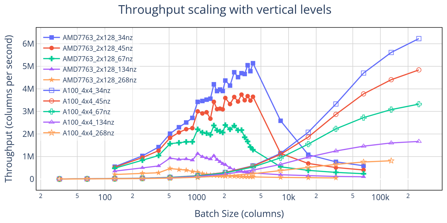
Figure 3 Throughput comparison between four NVIDIA A100 GPUs and two AMD 7763 CPUs using five different configurations of vertical levels. The number of vertical levels used is indicated by the value of “nz”. Increasing the number of vertical levels used causes CPU performance to drop off at smaller batch sizes, which in turn causes performance metrics to shift in favor of GPU execution.

Table 2 Observed performance metrics when comparing four NVIDIA A100 GPUs against two AMD 7763 CPUs, when modifying the number of vertical levels used in the run. The throughput plots that generated these metrics are shown in Fig. 3. Increasing the number of vertical levels increases the throughput ratio metrics, and decreases the crossover metrics – making GPU execution more compelling.

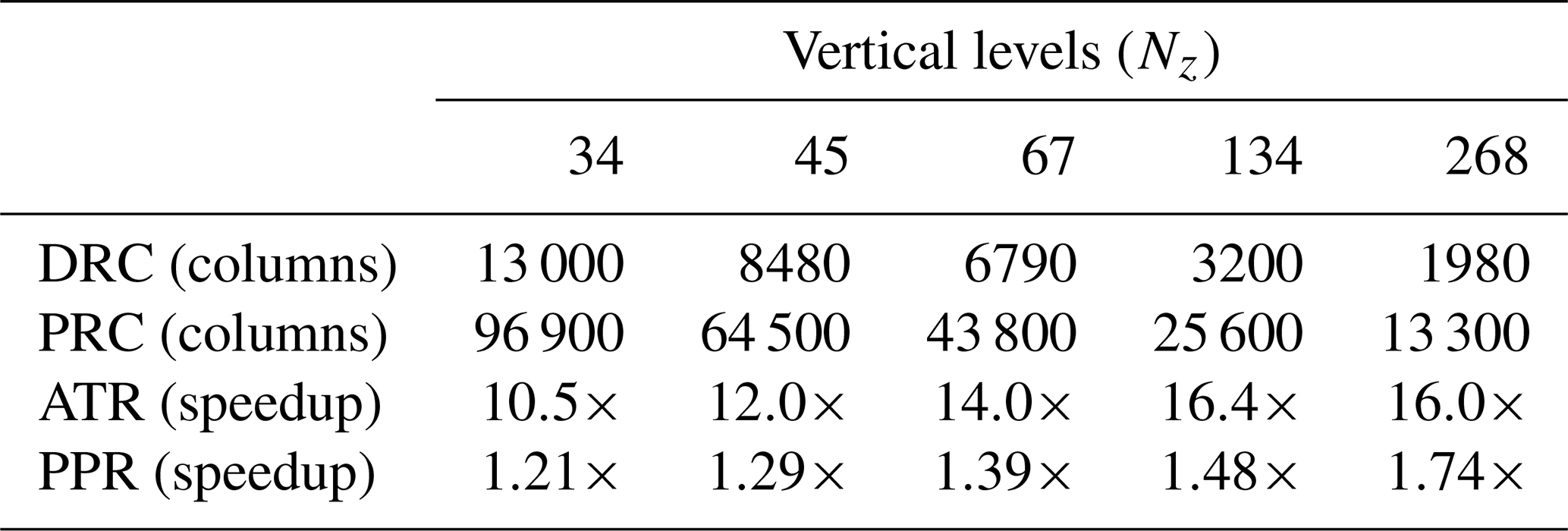
As vertical resolution increases, these metrics consistently shift in favor of GPU execution, illustrating how larger per-column workloads make GPUs increasingly advantageous. At the same time, the sensitivity of the results to vertical level count underscores that conclusions drawn from performance comparisons depend strongly on the chosen configuration – different vertical levels yield different numerical results and different performance metrics.

To make cross-configuration comparisons more stable and actionable, we reframe both throughput and batch size in terms of grid boxes – the product of columns and vertical levels – rather than columns alone. Expressing the results this way collapses much of the variability across vertical resolutions and enables simple extrapolation. For instance, Fig. 4 shows that the grid-box PRC remains close to 3.5 million across all cases, regardless of vertical level count. By dividing this grid-box PRC by an intended number of vertical levels – even one not directly tested – we can estimate a column-based PRC that would otherwise only be known after profiling, providing a practical way to decide in advance which device to run on.

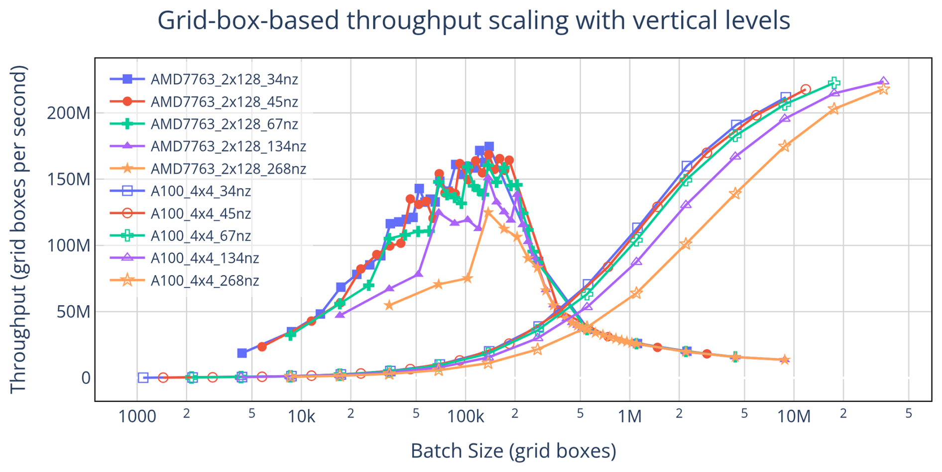
Figure 4 Plotting the data from Fig. 3 by redefining throughput and batch size in terms of grid boxes shows that the location of the CPU peak depends on both dimensions of work equally. This transformation does not affect the PPR or ATR, but results in tighter crossover metrics with the DRCs around 400–500 thousand grid boxes, and the PRCs around 3.5–4 million grid boxes. Specific values for the grid-box based metrics can be calculated by multiplying the metrics from Table 2 by the number of vertical levels used to generate them.

This framing also potentially supports rough extrapolation to other codebases. For example, RRTMGP (another atmospheric component written in a similar style to CLUBB) has a larger per-column workload defined by both vertical levels and radiation bands (Iacono et al., 2008). In principle, one could convert our grid-box PRC into a column-based PRC for RRTMGP by dividing by its per-column workload (vertical levels times radiation bands), yielding an estimate of its crossover point. However, such extrapolation is highly uncertain: algorithmic differences, larger memory footprints, and distinct memory access patterns all influence performance in ways that simple scaling cannot capture. Thus, while this may provide an estimate, we make no guarantees of its quality.

4.4 Runtime scaling

Although throughput is the more informative metric, visualizing raw runtimes can still yield valuable insights into performance scaling with batch size. When plotted this way, GPU runtimes exhibit a clear linear trend, while CPU runtimes may appear linear over a limited range before deviating into nonlinear behavior. This pattern is illustrated in Fig. 5, along with the linear trendlines described in Eq. (2) and Eq. (3).

$$\begin{array}{}\text{(2)}& {\displaystyle }{\widehat{R}}_{\mathrm{CPU}}\left(N_i\right)=\mathrm{6.877}\times {\mathrm{10}}^{-\mathrm{7}}\mathrm{s}{\mathrm{col}}^{-\mathrm{1}}\cdot N_i+\mathrm{3.111}\times {\mathrm{10}}^{-\mathrm{4}}\mathrm{s}\text{(3)}& {\displaystyle }{\widehat{R}}_{\mathrm{GPU}}\left(N_i\right)=\mathrm{5.667}\times {\mathrm{10}}^{-\mathrm{7}}\mathrm{s}{\mathrm{col}}^{-\mathrm{1}}\cdot N_i+\mathrm{8.049}\times {\mathrm{10}}^{-\mathrm{3}}\mathrm{s}\end{array}$$

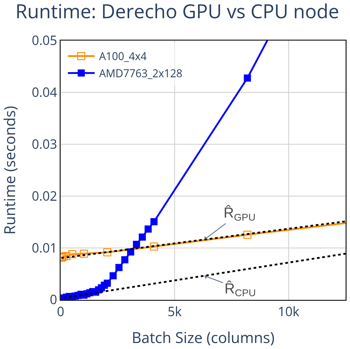
Figure 5 Average runtime of a single timestep, with linear trendlines overlaid. GPU runtime scales linearly with batch size – a trend that continues at large batch sizes not shown here. CPU runtime initially follows a roughly linear trend but diverges as the batch size increases. Note that despite this being the same data as in Fig. 1, the CPU peak is not visible here – highlighting the importance of visualizing throughput rather than raw runtime.

Modeling runtime this way allows us to analyze the fitted parameters and gain deeper insight into throughput behavior. In this example, the GPU has a much larger intercept – approximately 26× greater than the CPU – indicating a significantly higher baseline overhead and explaining why the CPU outperforms the GPU at small batch sizes. Although the trendline slopes are similar in this case, the CPU's apparent linear scaling breaks down at larger batch sizes, ultimately allowing the GPU to surpass it in performance.

These differences reflect fundamental architectural trade-offs. GPUs are designed to deliver massive parallelism but incur high latency costs (Andersch et al., 2015). CPUs, by contrast, prioritize low latency through caching hierarchies, branch prediction, pipelining, and out-of-order execution, making them well-suited for small workloads. However, as workload size increases and exceeds cache capacity, cache misses force reliance on slower memory tiers, leading to a steep drop in performance (Zhong et al., 2007).

This contrast also underscores the value of analyzing performance in terms of throughput. In Fig. 1, where performance is plotted as throughput, a distinct peak emerges for the CPU, representing the most efficient batch size for that device set. Such a peak is completely obscured when plotting raw runtime, emphasizing that throughput-based metrics are essential for identifying optimal configurations and for deriving our peak-based performance metrics like PPR and PRC.

5 Implementation results

In this section, we demonstrate the practical utility of the proposed performance metrics by applying them to a range of implementation choices. Whereas raw throughput comparisons can be sensitive to configuration details, our metrics distill these results into forms that are actionable and directly useful for guiding optimization. They highlight which decisions meaningfully affect performance while smoothing over minor complexities, allowing comparisons to remain both simple and robust.

5.1 Device and node comparisons

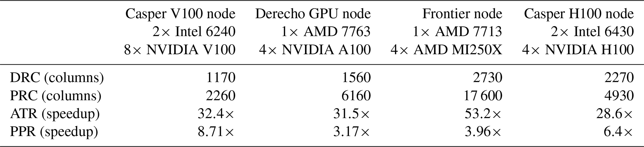
Comparing hardware across generations can be approached by plotting throughput on individual devices. Figure 6 shows results from single-device configurations – either one GPU or all cores of a single CPU – to ensure fair baselines for comparison. These single-device comparisons are useful for identifying broad performance trends, but they do not always translate into actionable insights. In practice, the number of devices available per compute node differs substantially: modern HPC nodes typically feature 1–2 CPUs but 4–8 GPUs.

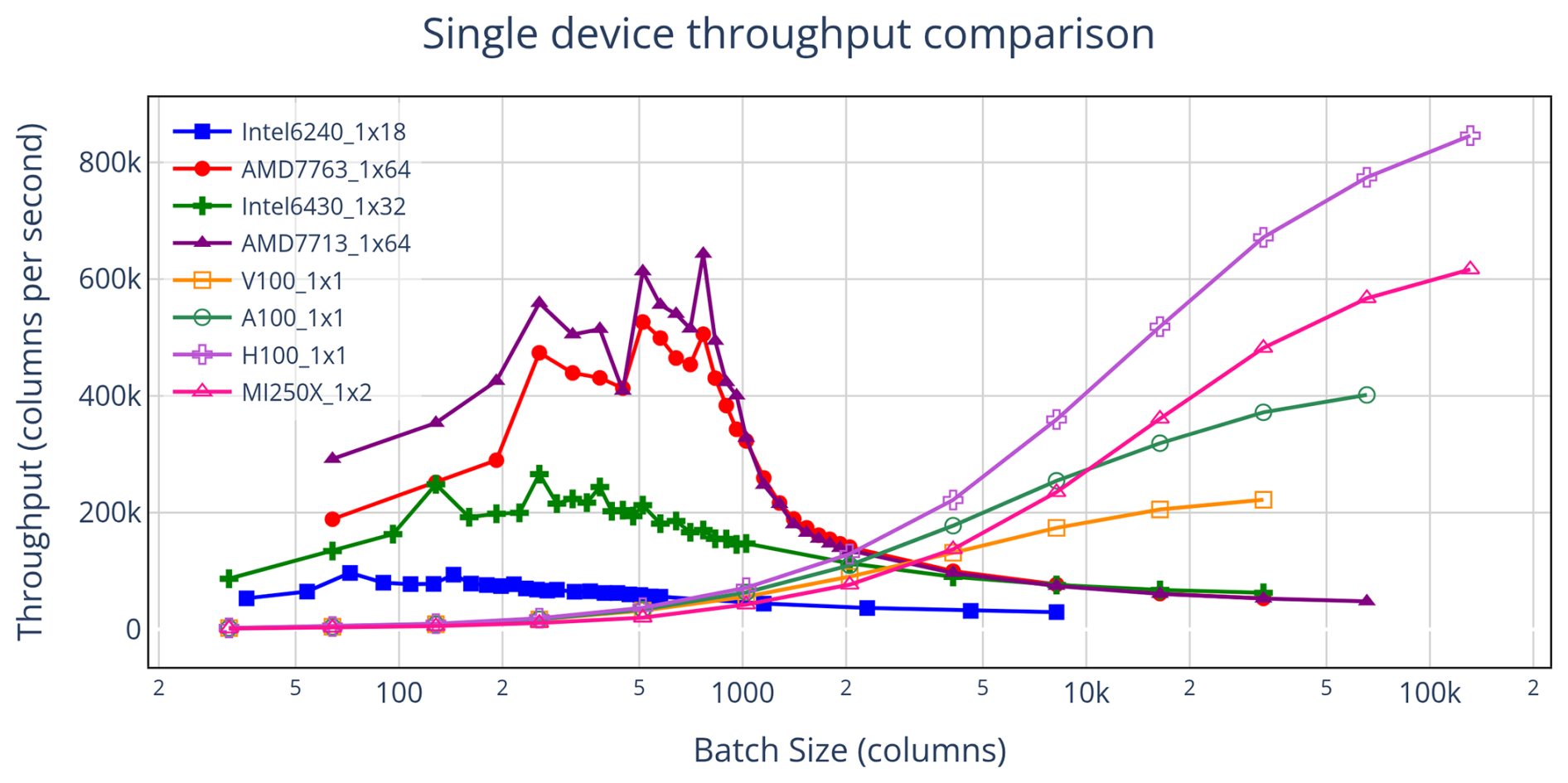
Figure 6 Throughput results for single-device configurations. Hardware specifics are detailed in Table 1. Performance varies substantially across devices, emphasizing that comparisons depend on the specific hardware rather than simply on device type (CPU vs. GPU). To be most fair, all GPU results were obtained without asynchronous directives (see Sect. 5.3), since our implementation of async failed with the crayftn compiler used for the MI250X.

To make comparisons more relevant, we focus on metrics from hardware within the same system. For example, Fig. 1 contrasts GPU and CPU nodes on the same cluster, where users must choose which resource to use. Table 3 shifts the focus to GPU nodes, reporting our performance metrics with each node evaluated in both CPU-only and GPU-only configurations. These metrics provide a practical basis for deciding whether to run workloads on CPUs or GPUs when both are available within a hybrid node.

Table 3 Performance metrics from fully utilized hardware configurations on GPU nodes, comparing CPU cores on those nodes to their resident GPUs. For the NVIDIA GPUs, asynchronous directives were used. Detailed hardware and software configurations are given in Table 1.

5.2 Single vs double precision

Scientific modeling software like CLUBB is typically compiled in double precision to maintain numerical accuracy, but when some accuracy can be sacrificed, single precision reduces the per-column data volume (workload) by roughly half at a fixed batch size, offering meaningful performance benefits. Figure 7 summarizes the effect. On CPUs, single precision improves performance mainly at larger batch sizes, consistent with reduced pressure on the memory hierarchy. On GPUs, the benefit is more pronounced and becomes evident at sufficiently large workloads; at the largest batch size tested, single precision is nearly twice as fast as double precision.

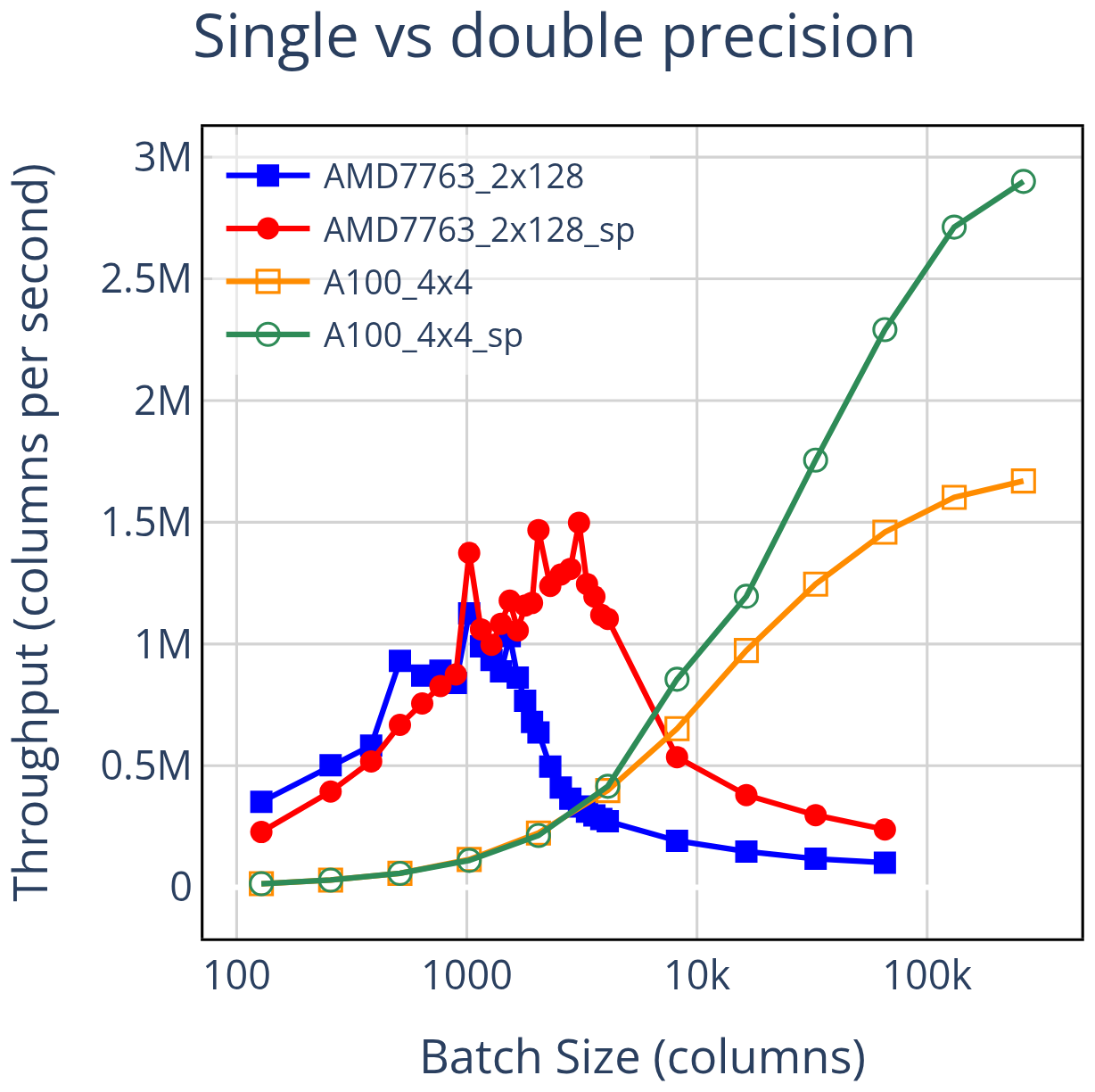
Figure 7 Comparing single vs. double precision performance with four NVIDIA A100 GPUs and two 64-core AMD 7763 CPUs. Single precision affects the performance scaling of the devices differently. This results in little change to the PRC, but a near doubling of the DRC, a shift favoring the CPU. The PPR, however, shifts in favor of the GPU, from 1.48× using double precision to 1.94× using single precision.

Applying our metrics clarifies an otherwise non-obvious conclusion. The PRC for single precision is similar to that for double precision, while the PPR is substantially larger. Single precision yields only modest gains at the mid-range workloads that matter most for the PRC, but much larger gains in the large workload regime used for the PPR. This illustrates the utility of the metrics: if the goal is to improve PPR (or ATR), using single precision is a strong option; if the focus is on PRC (or DRC), using single precision may offer limited benefit.

5.3 Asynchronous directives

GPU performance is degraded in part by CPU-GPU communication overhead, especially when each kernel launch forces the CPU to wait for completion. The OpenACC API provides async directives, which let the CPU enqueue GPU kernels without blocking (OpenACC-Standard.org, 2024). This creates a queue of work for the GPU and eliminates the need for synchronization events between kernel launches, thereby reducing the effective impact of kernel launch latency and keeping the GPU busy rather than idling. Figure 8 shows the throughput improvement from using asynchronous directives.

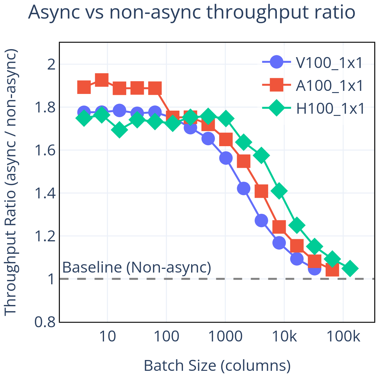
Figure 8 CPU-GPU synchronization costs can be significant when workloads are small. OpenACC async directives can be used to avoid most of these costs. The performance improvement is significant at small batch sizes, but has little effect at large batch sizes, where runtime is dominated by computation. This results in little effect on the PPR or ATR, but can significantly reduce the PRC and DRC.

To implement asynchronous directives, we launch almost all GPU kernels in the same stream using async(1). Using a single stream keeps the code maintainable, since it avoids the need to rebuild the dependency chain if the order of kernels changes. Although this choice prevents concurrent kernel execution, it still defers synchronization points and eliminates most launch-related stalls. A similar approach was taken in the GPU port of the ICON (Icosahedral Nonhydrostatic) model (Lapillonne et al., 2026).

Comparing GPU runs with and without async directives, we see substantial gains at small and mid-range batch sizes (where fixed latency costs matter) and little change at the largest batch sizes (where computation dominates). In metric terms, PRC and DRC improve, whereas PPR and ATR remain largely unchanged. This is the dual of the results in Sect. 5.2 where we compare the effect of numerical precision – there, single precision primarily increased PPR and ATR with little effect on PRC or DRC. Both results are elucidated by use of multiple metrics.

5.4 OpenACC vs OpenMP

When accelerating Fortran with directives, two primary options are OpenACC (OpenACC-Standard.org, 2024) and OpenMP (OpenMP.org/specifications, 2024). Although either option can, in principle, achieve similar performance, the realized results depend on source structure and the compiler's optimizations for the chosen model. Figure 9 compares the two options on NVIDIA GPUs using the nvfortran compiler, with OpenMP directives generated from the original OpenACC code via Intel's OpenACC Migration Tool (Intel, 2024).

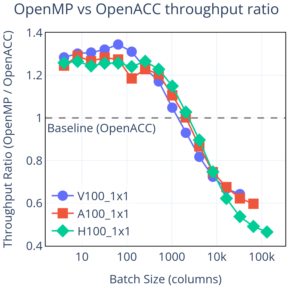
Figure 9 Throughput achieved using OpenMP directives relative to OpenACC. While OpenMP shows a slight advantage at small batch sizes, OpenACC delivers consistently better performance at all others. Importantly, when comparing these GPU results to the CPU results in Fig. 1, every performance metric we consider (PRC, DRC, PPR, ATR) favors OpenACC.

OpenMP shows a small advantage at the smallest batch sizes, but this reverses beyond roughly 2000 columns. At the largest batch sizes tested, OpenACC delivers up to approximately 50 % higher throughput. The OpenMP shortfall is concentrated in kernels that run substantially slower than their OpenACC counterparts, often where minor complexities (e.g., inner-loop data dependencies) are present. Similar scaling patterns – OpenMP declining relative to OpenACC at larger workloads – have been reported elsewhere on NVIDIA systems (Khalilov and Timofeev, 2021; Sun et al., 2023).

Our metrics contextualize the seemingly “mixed” outcome at small and large batch sizes. Because our metrics focus the comparison on batch-size ranges where GPUs are beneficial, they show that OpenACC has an overall advantage over OpenMP for this configuration. In this study, the OpenMP directives were generated from the OpenACC code using Intel's migration tool and compiled with the NVIDIA nvfortran compiler, so the comparison should be interpreted as specific to NVIDIA hardware and its compiler ecosystem. The small-batch cases where OpenMP appears faster lie outside the GPU-beneficial regime – there the CPU outperforms either GPU result – so those results do not factor into our actionable metric-based comparisons. In effect, the metrics smooth over these local quirks and clarify the advantage of OpenACC when GPUs are the appropriate hardware.

5.5 Miscellaneous implementation methods

In this subsection, we describe two implementation choices that, while not revealing new utility for the metric-based approach, are nevertheless worth noting.

The first concerns the choice of compiler. We used three in this work: Intel's ifx (Intel Corporation, 2024), NVIDIA's nvfortran (NVIDIA Corporation, 2024a), and HPE's crayftn (HPE Cray, 2024). See Table 1 for more on which compiler was used for each result. Because ifx cannot generate GPU code for either NVIDIA or AMD devices, it was used only for CPU results, where it produced performance comparable to crayftn and slightly ahead of nvfortran. For GPU code, both nvfortran and crayftn can target all devices tested. On the NVIDIA A100 GPUs with OpenACC and without async directives, crayftn consistently outperformed nvfortran across all batch sizes. Profiling with NVIDIA Nsight Systems (NVIDIA, 2025b) revealed that nvfortran-generated kernels often used more registers per thread, which reduces streaming multiprocessor (SM) occupancy due to the finite register file size, leading to underutilization of the hardware (NVIDIA Corporation, 2024b). By contrast, crayftn frequently produced kernels with lower register usage per thread, enabling higher occupancy and improved performance in several expensive kernels.

The second involves NVIDIA's Multi-Process Service (MPS) (NVIDIA Corporation, 2025). Running multiple MPI tasks per GPU can reduce idle time by hiding latencies, but because this is also the effect of asynchronous execution, the benefit of MPS depends on whether async directives are used. Without async directives, oversubscribing GPUs with tasks under MPS generally improved performance. With async directives, however, MPS tended to degrade performance at small to medium batch sizes, though it still offered a modest benefit at larger ones. An additional consideration with running extra tasks is memory usage: additional tasks increase the overall memory footprint, since certain variables must be duplicated across tasks. With one or two tasks per GPU we could accommodate up to roughly 65 536 columns per GPU (when using 134 vertical levels per column), but with more than two tasks, that same batch size exceeded available GPU memory.

6 Optimization analysis

Performance comparisons between CPUs and GPUs are often used by developers when deciding whether to GPUize their own codes. Earlier sections addressed fair reporting practices, but an equally critical factor is the level of optimization. While many optimizations benefit both devices (Govett et al., 2017), code structure can sometimes strongly advantage one architecture over the other (Lee et al., 2010). Because the heart of these comparisons is a performance ratio, uneven optimization can completely distort conclusions. A large reported GPU speedup may not reflect inherent GPU suitability at all – it may simply indicate that the CPU version was poorly optimized.

For readers considering GPUizing CLUBB-like codebases, it is therefore essential that our results represent a balanced optimization state, or at least make clear the source of any imbalance. Otherwise, our results risk conveying a misleading view of hardware capabilities. In this section, we first present a motivating example that shows how sensitive these metrics are to small structural changes. We then assess the broader optimization state of CLUBB on CPUs and GPUs, providing both a check on the fairness of our comparisons and a roadmap for reducing inefficiencies in future work.

6.1 Motivating example

For a practical example of how much performance metrics shift based on the level of code optimization, we zoom into the CLUBB code and analyze the performance of a specific matrix-solving algorithm. Among CLUBB's algorithms, this one is notable for containing a vertical dependency, where computations on one vertical grid level depend on results from the level below. Such dependencies prevent parallelism over the vertical dimension. By examining how throughput changes on each device as a result of loop reordering, we show that even a simple structural code change can produce drastically different performance outcomes.

In CLUBB, most computations involve two-dimensional loops over columns (the i-dimension) and vertical levels (the k-dimension). CLUBB arrays are dimensioned i-k, so the most cache-friendly and vector-friendly loop ordering in Fortran places the i-loop innermost. On CPUs, this arrangement is especially important, as it enables vectorization and efficient memory access.

GPUs, however, have different optimization priorities. For computations with k-loop dependencies, only the i-dimension can be parallelized across GPU threads. Placing the i-loop on the outside exposes this parallelism naturally, requiring just a single OpenACC directive and allowing full freedom inside the loop body. By contrast, putting the i-loop inside the k-loop still permits parallelism, but demands more complex OpenACC directives and may increase code complexity in ways that hurt performance. These conflicting constraints often force developers to favor one device over the other, or to rely on conditional compilation depending on the target device (Escobar et al., 2025).

One of CLUBB's matrix solver routines, penta_lu_solve_multiple_rhs_lhs, which employs an LU decomposition method (Walker et al., 1989), is particularly informative to analyze because it combines two notable features: it contains a vertical dependency that limits parallelism, yet its loop order can still be switched – something not always possible in data-dependent algorithms. Figure 10 presents its measured throughput before and after loop-order optimization. In the default form, the solver is optimized for GPUs, with the k-loop innermost, an arrangement that severely limits CPU performance. Refactoring the loop order to place the i-loop innermost restores CPU efficiency, but with the OpenACC directive left on the i-loop it fragments GPU work into many small kernel launches, reducing performance. This effect could be mitigated by more complex directive strategies, though we do not explore that here.

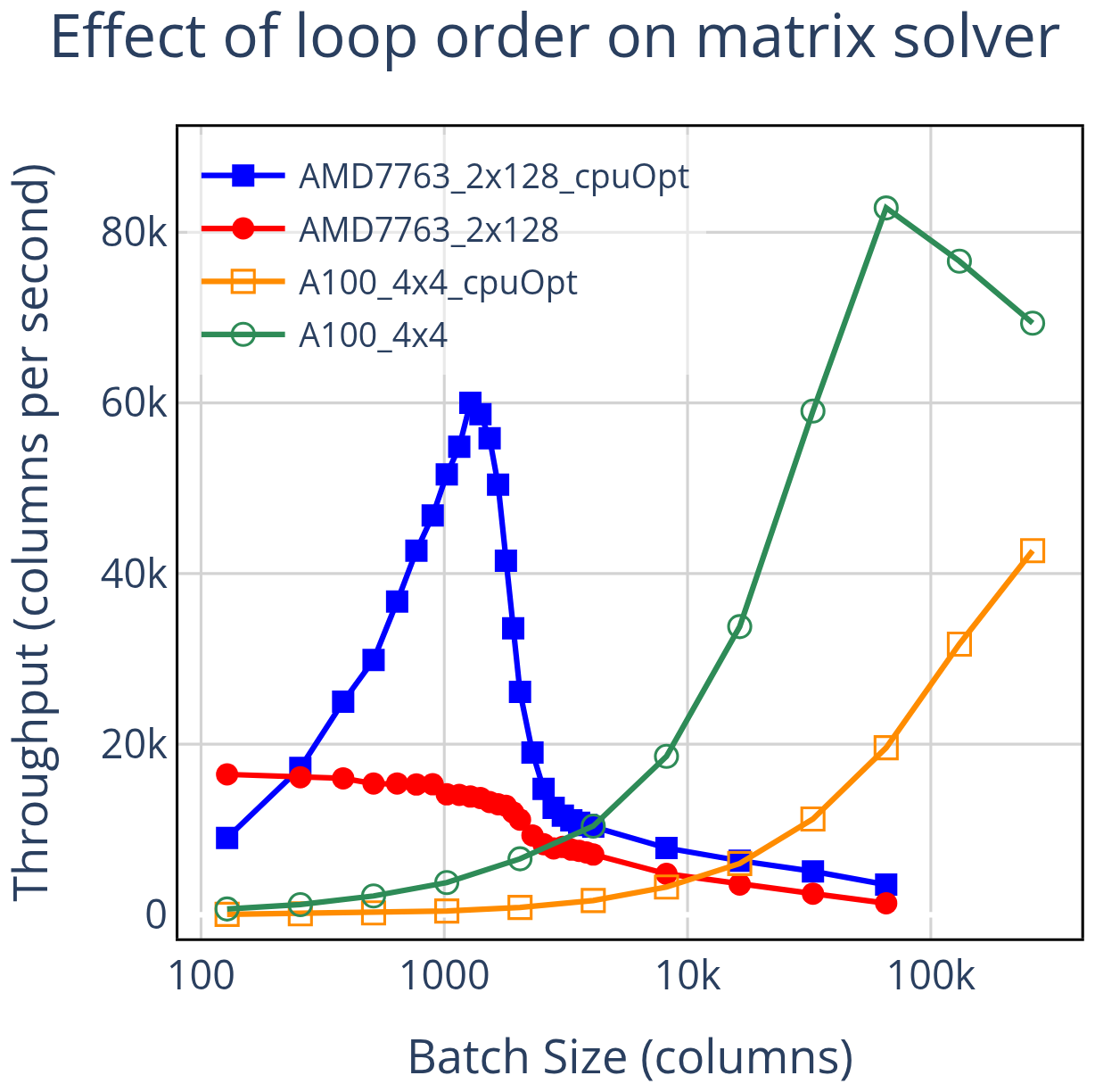
Figure 10 Throughput comparison of one of CLUBB's matrix solver routines before and after reordering loops. In the default GPU-oriented configuration, the PPR is 5×, and after reordering loops to favor CPU performance, the PPR drops to 0.71×, indicating the peak GPU throughput does not exceed peak CPU throughput. This demonstrates that optimization biases can drastically alter performance metrics.

This example shows how a small structural change can flip conclusions about which device is faster. In its GPU-oriented form, the matrix solver achieved a PPR of nearly 5×, suggesting a strong GPU advantage. After reordering to favor CPUs, the PPR fell below 1 (0.71×), indicating that the GPU never exceeds peak CPU throughput. The broader lesson is that CPU-GPU comparisons cannot assume comparable optimization: modest choices (e.g., loop order, directive placement) can bias results toward one architecture. More balanced approaches are often possible, but our aim here is to emphasize that performance comparisons are not always a neutral reflection of hardware capability or algorithmic suitability, and may instead reflect differences in optimization state.

6.2 CLUBB GPU efficiency

Analyzing GPU execution efficiency involves two key considerations: kernel performance (a kernel being a GPU-executed loop) and the amount of idle time when no kernels are running. Using NVIDIA Nsight Systems (NVIDIA, 2025b), we found no significant idle periods between kernels (not shown). The small time-gaps that do exist are due to infrequent synchronization events and minor memory transfers from reduction operations. Most kernel launch latency is avoided through the use of asynchronous directives – an important consideration given the large number of small kernels in CLUBB, explored further in Sect. 5.3. With idle time minimized, our focus shifts to kernel performance, which we analyze using a roofline diagram (Williams et al., 2009) generated with NVIDIA Nsight Compute (NVIDIA, 2025a).

Roofline

A single call to CLUBB consists of approximately 900 (non-unique) GPU kernels. Within CLUBB, there are relatively few runtime hotspots: some significant costs arise from small helper kernels that are invoked frequently, while others arise from infrequently executed kernels that are individually expensive. Figure 11 presents a roofline plot of every kernel launched in a single CLUBB timestep, as profiled on an NVIDIA A100 GPU.

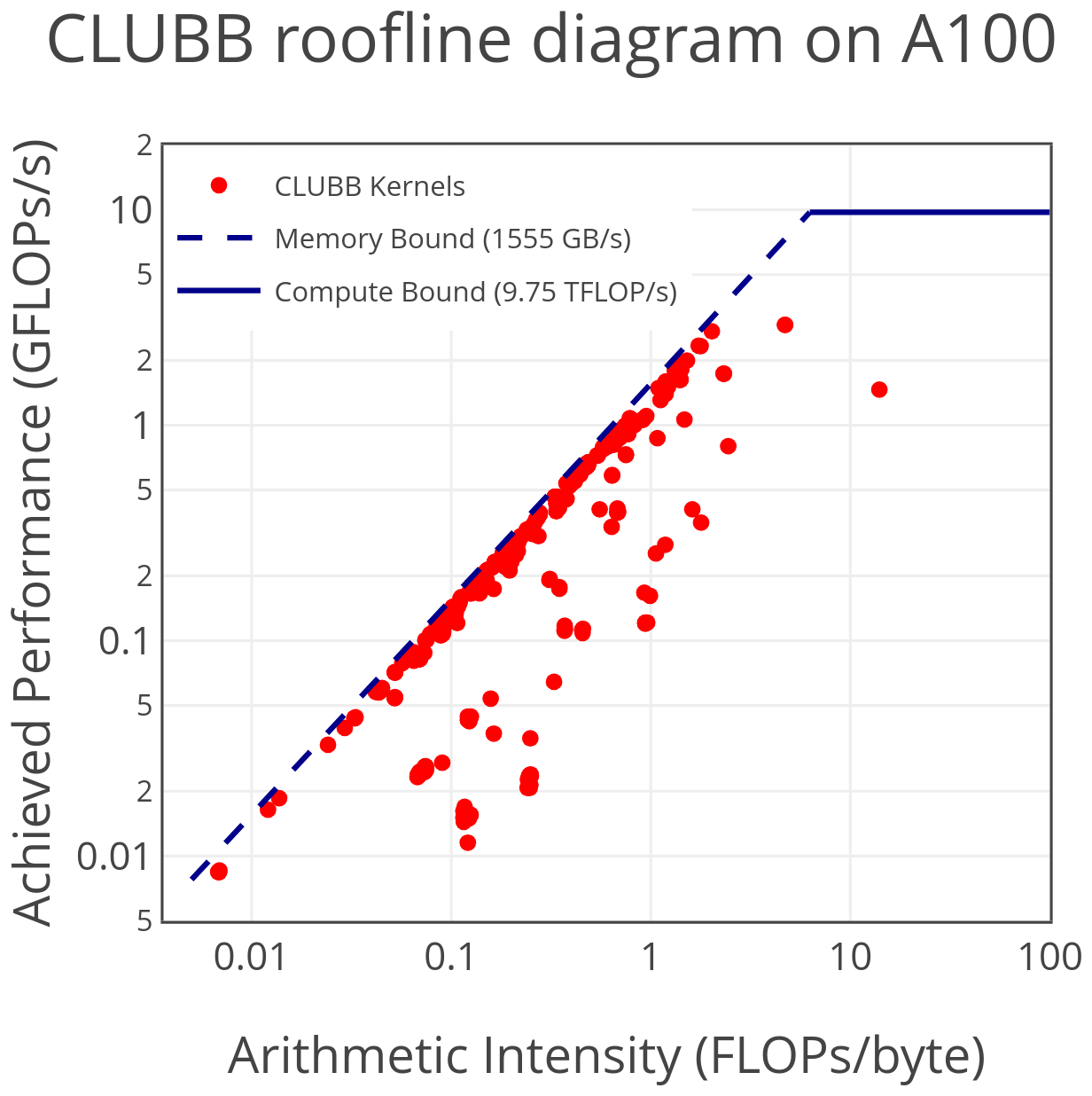
Figure 11 Roofline diagram of all CLUBB kernels run in a timestep. Approximately 900 kernels are depicted, mostly unique, but various helper routines are invoked multiple times per timestep. Profiled using NVIDIA Nsight Compute on an NVIDIA A100, running with 65 536 columns and 134 vertical levels.

To better understand kernel efficiency, we plot the ratio of achieved-to-theoretical peak performance, where the theoretical bound is determined by the arithmetic intensity of each kernel. In addition, we include a heatmap showing the fraction of total runtime accounted for by kernels within each bin. This helps highlight regions where future optimization may have the greatest impact. Figure 12 shows the data binned by efficiency, while Fig. 13 shows the same data binned by arithmetic intensity.

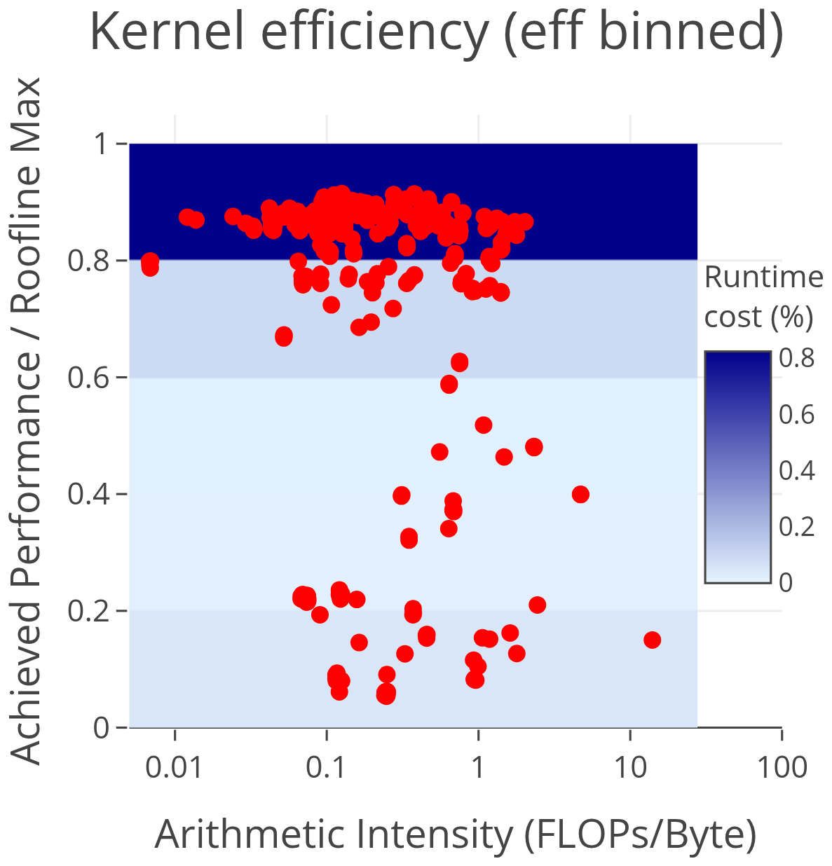
Figure 12 CLUBB kernel efficiency relative to roofline maximum. Overlaid is an efficiency binned heatmap of the runtime contribution of kernels. This shows that the majority of runtime cost on the GPU is from kernels that achieve near-peak efficiency – making it difficult to justify devoting effort to improving the performance of individual kernels.

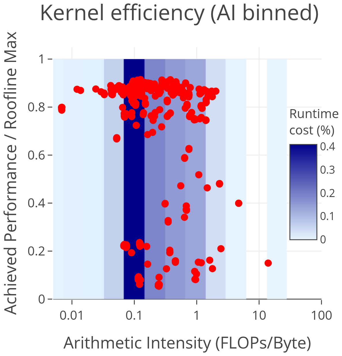
Figure 13 CLUBB kernel efficiency relative to roofline maximum. Overlaid is an arithmetic intensity binned heatmap of the runtime contribution of kernels. This shows that the majority of runtime costs on the GPU are from kernels with a relatively low arithmetic intensity – identifying a more promising target for future optimizations.

The efficiency-binned plot in Fig. 12 shows that 82 % of CLUBB's runtime is spent in kernels operating at ≥80 % of their theoretical maximum efficiency, with most clustering around 90 % efficiency. Only 8 % of the total runtime is attributable to kernels achieving 50 % efficiency or less. This suggests that focusing optimization efforts on underperforming kernels would yield limited benefit. Moreover, CLUBB has already gone through a round of GPU optimizations, and underperforming kernels with high costs have already been addressed. The remaining, individually expensive kernels implement algorithms that do not parallelize well, and improving them would require replacing them with fundamentally different algorithms. Conversely, targeting the highly efficient kernels is also hard to justify, as they are already near peak performance and offer little room for improvement.

The arithmetic intensity-binned plot in Fig. 13 shows that 49 % of the total runtime comes from kernels with arithmetic intensity ≤0.14, identifying a more promising target for optimization. To put this into perspective: if a kernel performs n total FLOPs (floating point operations), with one operation per double-precision (8-byte) value, its arithmetic intensity is $\frac{n\left(\text{FLOPs}\right)}{\mathrm{8}n\left(\text{bytes}\right)}=\mathrm{0.125}$ FLOPs byte⁻¹. This suggests that CLUBB kernels commonly perform little more than one operation per floating-point value. Increasing arithmetic intensity could be achieved by combining kernels that operate on common variables, thereby raising the maximum theoretical performance (Watkins et al., 2022). If we were able to double the arithmetic intensity of kernels in the ≤0.14 bins without reducing efficiency, we could double their performance and reduce total runtime by up to 24.5 %. Many of the low-intensity kernels in CLUBB originate from small helper routines, so in practice, increasing intensity would require either inlining and merging these routine calls or converting them into scalar routines that can be invoked directly within a GPU kernel.

6.3 CLUBB CPU efficiency

To give a sense of how well CLUBB is optimized on the CPU, we will consider two metrics – the vectorization ratio, and the cache miss rate. To profile these metrics, we used Intel's VTune (Intel Corporation, 2025) on a 64-core Intel 6430 CPU at varying batch sizes. The profiles themselves were gathered on only a single core, but to get the most accurate representation of these hardware metrics under full load, the other 63 cores were stressed by running repeated CLUBB runs at the same batch size as the profiled one, until the profile on the single core was complete.

The vectorization report gives us a sense of how well CLUBB is exploiting the vector units on the CPU. As explained at the beginning of this section, CPU code is only vectorized over the innermost loop, which for the vast majority of CLUBB code is the i-loop. This results in vectorization varying as we vary the number of columns. Since we are compiling with 256-bit vector calculations and double-precision (64-bit), each vector instruction can compute $\mathrm{256}/\mathrm{64}=\mathrm{4}$ operations at a time. As a result, we see spikes in the vectorization ratio at multiples of 4 columns. This also explains why we see spikes in the throughput plots every 4 data points (see Fig. 1) – it lands in a per-core batch size that causes our i-loops to be perfectly vectorized, resulting in a more performant run.

Figure 14 plots the portion of floating point instructions throughout CLUBB that are vectorized. At the highly vectorized batch sizes, CLUBB achieves roughly 67 % vectorization ratio, meaning that 67 % of the floating point operations are vector operations, and 33 % are scalar ops. There is some slight ambiguity in how one could report this – given that the vector operations are computing 4 floating point values per op, we could also consider the ratio of calculations that are computed using vector ops, which would result in a ratio of $\mathrm{4}\cdot \mathrm{67}/(\mathrm{33}+\mathrm{4}\cdot \mathrm{67})\approx \mathrm{89}$ %. A closer investigation into the origin of the scalar operations shows that they are all from a handful of code sections implementing algorithms that prevent vectorization – e.g. vertically dependent loops whose i-loop cannot be placed innermost.

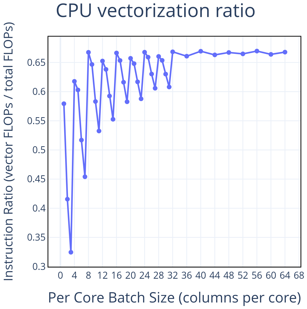
Figure 14 This shows the ratio of floating point operations that are vectorized to total floating point operations – profiled on an Intel 6430 CPU using Intel's VTune profiling tool. Compiling with double precision and 256-bit vector operations results in the best vectorization at multiples of 4 columns per core.

To investigate caching behavior, we use VTune metrics that report the number of clock cycles during which the CPU is stalled due to cache misses. In particular, MEMORY_ACTIVITY.STALLS_L1D_MISS, MEMORY_ACTIVITY.STALLS_L2_MISS, and MEMORY_ACTIVITY.STALLS_L3_MISS measure stalls resulting from L1 data cache, L2 cache, and L3 cache misses, respectively. Figure 15 shows these metrics across batch sizes, normalized to indicate the fraction of total cycles stalled at each cache level.

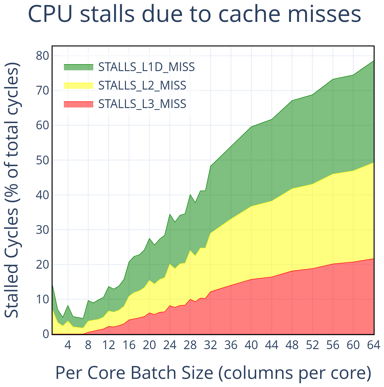
Figure 15 Tracking the number of CPU cycles that are stalled due to cache misses provides a high-level understanding of how much stress there is on the memory hierarchy. At small batch sizes, where the CPU performance peaks, caching is quite efficient. As the batch size increases, cache misses become increasingly frequent, causing stalls that drastically reduce the efficiency of the CPU.

These results provide insight into the efficiency of memory access patterns in CLUBB. As shown in Fig. 6, the Intel Xeon 6430 CPU reaches peak performance at eight columns per core. At these small batch sizes, fewer than 10 % of cycles are stalled by cache misses, with almost no contribution from L3. Performance begins to decline once L3 misses become significant, and as batch size increases further, stalls from all cache levels grow steadily, approaching 80 % of cycles at the largest size tested. This indicates that the observed drop-off in throughput is primarily driven by increasing pressure on the memory hierarchy.

Improving CPU performance would require progress in either vectorization or memory usage. While CLUBB is already heavily vectorized, further gains could in principle be achieved by replacing non-vectorizable algorithms with alternative formulations that lend themselves better to vectorization. Such changes, however, are nontrivial, as they typically involve introducing algorithms that are both mathematically equivalent and numerically stable. Artificially forcing vectorization without algorithmic changes is unlikely to yield meaningful improvements and may be impractical (Shen et al., 2018). Alternatively, optimizations that reduce memory stress, such as improving data locality to better utilize caches, could also be considered (Zhong et al., 2009). Yet because cache behavior is already efficient at the batch sizes where peak throughput occurs, such optimizations would likely not substantially raise peak performance. Their main effect would be to sustain high throughput across slightly larger batch sizes, with limited influence on peak-based metrics such as PPR or PRC. Consequently, there are no clear optimization targets that would meaningfully improve CPU competitiveness.

7 Discussion on the viability of exploiting peak performance

One distinguishing aspect of this work is our focus on peak CPU performance. In Sect. 4.2, we introduced the Peak-to-Peak Ratio (PPR) and Peak Ratio Crossover (PRC), showing how batch-size tuning can make CPUs highly efficient for problems that can be freely subdivided. However, in Sect. 4.3 we demonstrated that the batch size which yields peak CPU throughput can shift with non-tunable workload factors. Then in Sect. 6 we showed that the prominence of this peak depends strongly on CPU-specific optimizations. These findings raise a key question: how viable is it to exploit the CPU peak in practice?

Exploiting the CPU peak we observe in CLUBB standalone requires a lightweight driver that partitions work across cores and repeatedly executes small batches while amortizing start-up costs. Because CLUBB's columns are independent, such a driver is feasible in principle; similar distribution mechanisms exist in host models that embed CLUBB (Worley and Drake, 2005).

CLUBB's pronounced CPU peak reflects its homogeneity: the computations are dominated by two-dimensional loops over columns and vertical levels, most of which are vectorized and memory-contiguous. As a result, most code sections attain their best CPU performance at the same batch size. By contrast, other physics components may have a larger per-column workload – e.g., radiation such as RRTMG (Mielikainen et al., 2016) adds a band dimension – so RRTMG's CPU-optimal batch size will differ from CLUBB's (see Sect. 4.3 for more on the effect of modifying the per-column workload). In a coupled model containing both CLUBB and RRTMG, exploiting each component's peak would therefore require a driver that supports different per-component batch sizes. More generally, even within a single, non-component code, different sections may prefer different batch sizes, making any single choice of batch size potentially suboptimal.

When executing on GPUs, these complications are far less pronounced. For a given device, the throughput-maximizing batch size is typically the largest size that fits in device memory. Because this memory limit applies uniformly across the coupled model, a single (memory-limited) batch choice aligns the ideal workload across components and obviates the need for different per-component batch sizes and the coordinating driver logic they would require on CPUs. This global alignment of the ideal batch size is a practical advantage of GPUs that can be obscured when profiling a single homogeneous code such as CLUBB.

8 Conclusions

To address some challenges of interpreting CPU-GPU performance comparisons, we have introduced two new performance metrics in Sect. 4.2. These peak-based metrics, Peak Ratio Crossover (PRC) and Peak-to-Peak Ratio (PPR), are particularly valuable for problems that can be broken down into smaller workloads, such as the CLUBB standalone model that we consider throughout this work. These metrics enable us to answer questions about which device is preferable given our problem size. The PRC answers the question: Given an integer N, will running CLUBB standalone on a total of N columns be faster on CPUs or GPUs? The PPR answers the question: Given a very large N, how much faster will the GPUs be compared to the CPUs?

Our main comparison pits the hardware on a Derecho CPU node (two 64-core AMD EPYC 7763 CPUs) against the hardware on a Derecho GPU node (four NVIDIA A100 GPUs) (see Fig. 1), which are the two types of node found within the Derecho cluster. In this comparison, we find a PRC of 25 600 columns and a PPR of 1.48×. The PRC tells us that when we have the choice of running CLUBB standalone on one of these particular hardware sets, GPU execution is preferable when the problem size exceeds 25 600 columns per node, and CPU execution is preferable for any smaller problem size. The PPR tells us that for very large problem sizes (exceeding 256 000 columns per node), GPU execution results in a 1.48× speedup over CPU execution.

The more traditional performance metrics discussed – the Direct Ratio Crossover (DRC) and the Asymptotic Throughput Ratio (ATR) – are not directly relevant to CLUBB standalone when considering performance as a function of batch size, but would answer those same questions for a problem that cannot be broken down into smaller workloads. Additionally, the large differences observed between our peak-based metrics and the direct metrics make clear the importance of considering a code's ability to batch computations. Had we not considered the capability of CLUBB to break our problem (an overall number of columns to process) up into smaller workloads (batches of columns), we would have ended up overstating the performance benefit of GPU execution.

In Sect. 4.3, we show that accounting for the per-column workload generalizes throughput and enables prediction (for untested configurations) of the workload at which CPU performance peaks. This framing also potentially supports extrapolation of our results to codes with CLUBB-like characteristics (highly parallelizable and memory-bound) that differ in their per-column workloads.

In Sect. 5, we evaluate how our metrics clarify performance differences and can be used to guide implementation choices. For example, Sect. 5.3 shows that adding asynchronous OpenACC directives markedly reduces PRC with little effect on PPR, whereas Sect. 5.2 shows that switching to single precision substantially increases PPR while leaving PRC largely unchanged. Thus, to reduce the PRC, incorporating asynchronous directives may be a better investment of effort, while increasing the PPR may be better achieved by enabling single-precision builds.

In Sect. 6, we showed that effective optimization strategies can conflict between CPUs and GPUs, so headline speedups are not a pure measure of hardware capability. A large GPU/CPU “speedup” does not, by itself, imply the code is inherently “well-suited” to GPUs; it can equally reflect under-optimized CPU code. This raises a central question: does CLUBB's structure favor either device? To answer it, we analyzed how efficiently each architecture is utilized in Sects. 6.2 and 6.3. We found that CLUBB standalone is already well-optimized for both architectures, but appears to leave greater untapped performance potential on GPUs.

Overall, our results show that GPUs offer compelling performance advantages for HPC applications like CLUBB standalone, but interpreting performance comparisons requires care. The metrics we introduce highlight the most important aspects of these comparisons, helping answer specific performance questions and revealing that, for problems that can be processed in batches of smaller workloads, CPUs can be more competitive than raw performance differences suggest. However, as discussed in Sect. 7, there are practical challenges in fully exploiting CPU performance, further reinforcing the appeal of GPU execution.