On moist ocean-atmosphere coupling mechanisms

We investigate mechanisms governing moist energy exchanges at the atmosphere-ocean interface in global Earth system models. The goal of this work is to overcome deficiencies like energy fixers and unphysical thermodynamic formulations and designs that are commonly used in modern models. For example, while the ocean surface evaporation is one of the most significant climatological drivers, its representation in numerical models may not be physically accurate. In particular, existing schemes give an incorrect atmospheric air temperature tendency during evaporation events. To remedy this, starting from first principles, we develop a new mechanism for the ocean-atmosphere moist energy transfers. It utilizes consistent thermodynamics of water species, distributes latent heat of evaporation in a physically plausible way, and avoids reliance on artificial energy fixers. The temperature and water mass tendencies are used to formulate a set of ordinary differential equations (ODEs) representing a simple box model of ocean-air exchange. We investigate the properties of the ODEs representing the proposed mechanism and compare them against those derived from the current designs of the Energy Exascale Earth System Model (E3SM). The proposed simplified box model highlights the advantages of our approach in capturing physically appropriate atmospheric temperature changes during evaporation while conserving energy.

1 Introduction

The purpose of this work is to investigate mechanisms of latent heat transfer due to evaporation at the ocean-atmosphere interface in climate models. Alongside radiation, the energy fluxes associated with precipitation and evaporation are one of the largest contributors to the Earth climate patterns (Trenberth et al., 2009; Stevens and Schwartz, 2012). A recently published overview (Lauritzen et al., 2022) highlights major deficiencies in the thermodynamic formulations used in the numerical climate models. One of the most significant issues in the models is incorrect representation of the internal energy of water forms in the atmosphere, which leads to errors in the energy footprint of evaporation and precipitation at the atmosphere-ocean interface.

There has been recent research into modeling consistent unapproximated thermodynamics for both the atmospheric (Eldred et al., 2022; Guba et al., 2024) and the ocean (Mayer et al., 2017) components of the models. Unlike many current designs that assign dry heat capacities to all forms of water in the atmosphere, the unapproximate thermodynamics uses close to theoretically established values specific to each water form. Therefore, there are large discrepancies between current designs and designs based on the unapproximated thermodynamics in representing energy fluxes. For example, enthalpy, defined with phase-appropriate specific heat capacities (Vallis, 2017; Eldred et al., 2022), is regarded as a valid representation of the biggest source of energy fluxes at the lower boundary of the atmosphere (Lauritzen et al., 2022; Guba et al., 2024). Using enthalpy based on unapproximated specific heats of water vapor ($c_{\mathrm{p}}^{\mathrm{v}}=\mathrm{1870}$ J kg⁻¹ K⁻¹ as defined by Emanuel, 1994) and liquid water (c_l=4190 J kg⁻¹ K⁻¹), instead of the specific heat of the dry air ($c_{\mathrm{p}}^{\mathrm{d}}=\mathrm{1005.7}$ J kg⁻¹ K⁻¹), alters the energy signal of water forms by a factor two to four.

Although many of these inconsistencies are patched using global energy fixers and pressure adjustments (Lauritzen and Williamson, 2019; Golaz et al., 2022; Guba et al., 2024), we argue that such approaches mask the underlying problems and limit the fidelity of Earth system models. As model resolution increases and we seek higher accuracy in regional and process-level predictions, continued reliance on artificial fixers becomes increasingly problematic.

In this work, we discuss one of the energy fixers, called IEFLX (Golaz et al., 2022), used in the Earth Exascale Energy System Model (E3SM) (Golaz et al., 2019, 2022) and in its atmospheric component, the E3SM Atmosphere Model (EAM) (Rasch et al., 2019). We explain how it restores the energy budget associated with latent heat fluxes from evaporation and precipitation at the atmosphere-ocean interface. While IEFLX balances the energy budget in E3SM, as we show, it does not model latent heat transfers in a physically consistent manner. This deficiency may potentially hinder Earth system models' fidelity and capabilities as the community transitions to use high-resolution and regional models.

Previously, in Guba et al. (2024), we analyzed precipitation mechanisms with consistent unapproximated thermodynamics. Since there is a delicate balance between climatological (long time-scale) energy trends of precipitating and evaporating fluxes at the atmosphere-ocean interface, it is not possible to redesign a numerical climate model gradually, by addressing only one or the other flux first. Instead, improvements in model thermodynamics must be applied to both evaporation and precipitation mechanisms simultaneously, even though they are often controlled by different components of the model. Therefore, this work, which focuses on both evaporative and precipitating mechanisms relevant to the atmosphere within a framework of unapproximated thermodynamics, is a natural extension of Guba et al. (2024).

Here, we investigate evaporation from the ocean surface as modeled in E3SM. We dive into the details of how the latent heat of evaporation is handled in E3SM with the help of global energy fixers, and how it could be instead redistributed using the unapproximated thermodynamics without fixers. We argue that the transfer of latent heat from evaporation across the atmosphere-ocean interface is not modeled in a physically plausible manner. To clarify the impact of these formulations, we implement three simplified numerical box models: one using consistent, unapproximated thermodynamics, and two mimicking E3SM-like assumptions. These models describe the temperature and water mass tendencies in the ocean and atmosphere using a system of four coupled ordinary differential equations, representing the evolution of atmospheric and oceanic water mass and temperature over time. The ocean and atmosphere are each represented as a single, well-mixed box. We show that the model based on consistent thermodynamics produces a different atmospheric temperature tendency during evaporation compared to the E3SM-like models. See Sect. 3.4.5 for details.

The overarching goal of this work is to further investigate deficiencies in thermodynamic approaches in current Earth system models. It aims to direct the Earth system modeling community toward the development of more physically and numerically consistent models by reducing reliance on crude approximations and artificial fixers. We emphasize that this study does not suggest that using the unapproximate thermodynamics in precipitation and evaporation would affect climatological biases in the current numerical Earth system models in any particular way. Such biases are often managed through extensive parameter tuning to match observations, and this tuning will likely remain necessary, even with improved physical foundations, for the foreseeable future. Nevertheless, we argue that the advances such as that proposed here can reduce the burden on practitioners to rely on such ad hoc tuning and enable more interpretable, transparent models grounded in sound physical and mathematical principles.

2 Overview and motivation

2.1 Moist physics in Earth system models: evaporation and condensation

The motivation for this work is two-fold. First, we aim to raise awareness about crude thermodynamic approximations commonly employed in the modern global Earth system models. In particular, in their atmospheric components and at the surface interfaces for water species models use specific heats of dry air instead of experimentally established specific heats of water forms. Second, we propose conceptual improvements intended to enhance the physical fidelity of these models.

For the purpose of this work, we separate moist physics at the ocean-atmosphere interface into two simplified categories: condensation and evaporation. For condensation, we consider processes that lead to precipitation. In climate models, such processes are typically represented by micro- and macro-physical parametrizations (see, e.g., Klemp and Wilhelmson, 1978; Morrison and Gettelman, 2008; Morrison and Milbrandt, 2015a; Golaz et al., 2002). For evaporation, we consider only the flux of water vapor from the ocean surface into the atmosphere. Such processes are often modeled by so-called bulk schemes (Haidvogel and Bryan, 1993) based on Monin-Obukhov Similarity Theory (MOST) (Shaw, 1990). Our simplified treatment of condensation and evaporation focuses on the thermodynamics at the ocean–atmosphere interface. In reality – and in more complex model implementations – these processes are not confined neatly to either the ocean or the atmosphere. For example, a condensed water droplet may remain suspended in the atmosphere or evaporate before reaching the lower boundary of the atmosphere. In our simplified framework, however, we assume that all condensed water mass in the atmosphere is transported directly to the ocean.

The thermodynamic aspects of condensation, along with possible improvements and their implications, were previously discussed by Guba et al. (2024). This work shifts focus to evaporation and the combined effects of evaporation and condensation. As further discussed in Sect. 2.2.4, while bulk schemes compute mass and temperature fluxes at the atmosphere-ocean interface, they do not account for energy transfers associated with evaporation. Instead, these transfers are modeled separately within the ocean and the atmosphere components of the model. In the following section, we examine the mechanisms governing these evaporative energy transfers in detail, because they provide a clear motivation behind this work.

2.2 Motivation: Closer look at energy transfers during evaporation

2.2.1 An overview of definitions and assumptions

In Sect. 3 we will introduce three sets of simple models – two of these are based on the implementation of the ocean and atmosphere thermodynamics in E3SM, and one representing an idealized implementation using unapproximated thermodynamics in both components. In all models, the ocean and the atmosphere components are represented by mean grid values for species mass and temperature. Before we get into the details of derivations in Sect. 3, we first motivate for our work by conceptually examining evaporation at the ocean-atmosphere interface.

Evaporative mechanisms at the ocean-atmosphere interface are incredibly complex (Niiler, 1993; Feistel and Hellmuth, 2023). While evaporation is ultimately driven by solar radiation (Trenberth et al., 2009), the net evaporative flux is influenced by a combination of external heating, the thermodynamic and dynamic states of both the atmosphere and the ocean, mixing processes, and even photomolecular effects (Tu et al., 2023).

Here, we focus only on a highly simplified version of one of these mechanisms, namely, the transfer of energy during evaporation from the ocean surface, in the absence of external heating (i.e., we assume that radiative energy fluxes preceding evaporation have already been absorbed by the ocean) or dynamical effects (no mixing or surface winds).

Consistent with the common practice in atmospheric modeling, we will reduce the conservation of energy to conservation of enthalpy (Lauritzen et al., 2022; Guba et al., 2024; Yatunin et al., 2026). Consider for simplicity the case of the dry air for a pressure-based model. The conserved “energy”¹ for a dry atmosphere with a pressure top can be written as

$$E_{\text{dry air}}=\iiint (e_{\text{kin}}+c_{\mathrm{v}}^{\mathrm{d}}T+gz)\mathit{\rho }\mathrm{d}V+\iint (pz{)}_{\text{top}}\mathrm{d}A.$$

Under the assumptions of a shallow, hydrostatic atmosphere this can be rewritten (Lauritzen et al., 2022) in terms of enthalpy as

$$\begin{array}{rl}{E}_{\text{dry air}}& =\iiint (e_{\text{kin}}+c_{\mathrm{v}}^{\mathrm{d}}T+gz)\mathit{\rho }\mathrm{d}V+\iint (pz{)}_{\text{top}}\mathrm{d}A\\ & =\iiint (e_{\text{kin}}+c_{\mathrm{p}}^{\mathrm{d}}T)\mathit{\rho }\mathrm{d}V+\iint (pz{)}_{\text{bottom}}\mathrm{d}A.\end{array}$$

It is important to note that $e_{\text{kin}}+c_{\mathrm{p}}^{\mathrm{d}}T$ is not an energy density, and that the integral of this term is not the total energy. Here e_kin is specific kinetic energy, T is temperature, $c_{\mathrm{v}}^{\mathrm{d}}T$ is internal energy, $c_{\mathrm{p}}^{\mathrm{d}}T$ is enthalpy, $c_{\mathrm{v}}^{\mathrm{d}}$ and $c_{\mathrm{p}}^{\mathrm{d}}$ are specific heat capacities for the dry air with respect to constant volume and constant pressure, p is pressure, ρ is density, z is height, and dV and dA are volumetric and surface measures. As shown in Lauritzen et al. (2022), in particular, in Fig. 3, most of the energy transfers between the atmosphere and the ocean corresponds to the change of enthalpy, not energy. Separately, using again the case of the dry air for simplicity, the first law of thermodynamics for change of internal energy is written as $\mathrm{d}u=-p\mathrm{d}\mathit{\alpha }+\dot{Q}$, where $u=c_{\mathrm{v}}^{\mathrm{d}}T$ is internal energy, $\mathit{\alpha }=\mathrm{1}/\mathit{\rho }$, and $\dot{Q}$ is external heat flux. The first law also can be reformulated in terms of enthalpy $h=c_{\mathrm{p}}^{\mathrm{d}}T$ as $\mathrm{d}h=\mathit{\alpha }\mathrm{d}p+\dot{Q}$. Most atmospheric physics packages, including those used in E3SM, are formulated for pressure-based vertical coordinates and make the assumption that the physics processes are isobaric. In that case, using the first law of thermodynamics in terms of enthalpy is the correct choice, and it is the one adopted in this paper.

In the unapproximated case, in both ocean and atmosphere, the enthalpy of water vapor with respect to ice reference state is given by Lauritzen et al. (2022), Eq. (64), $h^{\mathrm{v}}=\left(c_{\mathrm{p}}^{\mathrm{v}}\right(T-T_{\mathrm{00}})+h_{\mathrm{00}}^{\text{ice}}+L_{\mathrm{s},\mathrm{00}})m^{\mathrm{v}}$ and that of liquid water by $h^{\mathrm{l}}=\left(c_{\mathrm{l}}\right(T-T_{\mathrm{00}})+h_{\mathrm{00}}^{\text{ice}}+L_{\mathrm{f},\mathrm{00}})m^{\mathrm{l}}$, with $h_{\mathrm{00}}^{\text{ice}}=\mathrm{0}$ (therefore, omitted below). Here T is temperature, m^v and m^l are vapor and liquid water masses, $c_{\mathrm{p}}^{\mathrm{v}}$ is the specific heat capacity of the water vapor with respect to pressure, c_l is the specific heat capacity of the liquid water, and T₀₀=273.16 K is a reference temperature. In the current setup, whether we are using specific or mass-weighted enthalpies will be obvious from the context, and thus, we omit this distinction in the text. The constants $L_{\mathrm{s},\mathrm{00}}=L_{\mathrm{v},\mathrm{00}}+L_{\mathrm{f},\mathrm{00}}$ and L_f,00, where $L_{\mathrm{v},\mathrm{00}}=\mathrm{2.501}\times {\mathrm{10}}^{\mathrm{6}}$ and $L_{\mathrm{f},\mathrm{00}}=\mathrm{3.3337}\times {\mathrm{10}}^{\mathrm{5}}$ J kg⁻¹ are the latent heats of vaporization and fusion at T₀₀, represent the energy associated with molecular bonds. These constants should not be confused with the concept of latent heats, which is discussed below. For simplicity, we expand expressions h^v and h^l,

$$\begin{array}{rl}{h}^{\mathrm{v}}& =\left(c_{\mathrm{p}}^{\mathrm{v}}\right(T-T_{\mathrm{00}})+L_{\mathrm{v},\mathrm{00}}+L_{\mathrm{f},\mathrm{00}})m^{\mathrm{v}}\\ & =(c_{\mathrm{p}}^{\mathrm{v}}T+L_{\mathrm{v}}+L_{\mathrm{l}})m^{\mathrm{v}}\end{array}$$

and

$$h^{\mathrm{l}}=\left(c_{\mathrm{l}}\right(T-T_{\mathrm{00}})+L_{\mathrm{f},\mathrm{00}})m^{\mathrm{l}}=(c_{\mathrm{l}}T+L_{\mathrm{l}})m^{\mathrm{l}}$$

with

$$\begin{array}{rl}& L_{\mathrm{v}}:=L_{\mathrm{v},\mathrm{00}}-(c_{\mathrm{p}}^{\mathrm{v}}-c_{\mathrm{l}})T_{\mathrm{00}}=\mathrm{3.1}\times {\mathrm{10}}^{\mathrm{6}}{\text{J\hspace{0.17em}kg}}^{-\mathrm{1}},\\ & L_{\mathrm{l}}:=L_{\mathrm{f},\mathrm{00}}-c_{\mathrm{l}}{T}_{\mathrm{00}}=-\mathrm{8.1}\times {\mathrm{10}}^{\mathrm{5}}{\text{J\hspace{0.17em}kg}}^{-\mathrm{1}}.\end{array}$$

In many models, like EAM, the atmosphere uses the assumption that heat capacities for water species are the same as for the dry air. In Lauritzen et al. (2022) it is discussed that in this case there is no need to carry T₀₀ terms in energy formulation. However, the ocean thermodynamics in E3SM uses the specific heat capacity of liquid water, c_l. While this means the argument for the absence of T₀₀ in the energy formulation in Lauritzen et al. (2022) does not apply to E3SM, its implementation does not have associated with T₀₀ terms. When using thermodynamic models based on E3SM implementations, we will follow the model realizations exactly. In the atmospheric component of E3SM, EAM, the enthalpies of vapor and liquid water are given by $h_{\text{approx.}}^{\mathrm{v}}=(c_{\mathrm{p}}^{\mathrm{d}}T+L_{\mathrm{v}}^{\text{dry}}+L_{\mathrm{l}}^{\text{dry}})m^{\mathrm{v}}$ and $h_{\text{approx.}}^{\mathrm{l}}=(c_{\mathrm{p}}^{\mathrm{d}}T+L_{\mathrm{l}}^{\text{dry}})m^{\mathrm{l}},$ with $L_{\mathrm{v}}^{\text{dry}}=L_{\mathrm{v},\mathrm{00}}$ and $L_{\mathrm{l}}^{\text{dry}}=L_{\mathrm{f},\mathrm{00}}$.

Latent heats are defined as differences of specific enthalpies. For example, the latent heat of vaporization is defined as the difference h^v−h^l (in case of unapproximated thermodynamics) or $h_{\text{approx.}}^{\mathrm{v}}-h_{\text{approx.}}^{\mathrm{l}}$ in case of the EAM thermodynamics. It is discussed in detail in Lauritzen et al. (2022) that unapproximated thermodynamics corresponds to the case of variable latent heats, while thermodynamics that uses $c_{\mathrm{p}}^{\mathrm{d}}$ in $h_{\text{approx.}}^{\mathrm{v}}$ and $h_{\text{approx.}}^{\mathrm{l}}$ corresponds to the case of constant latent heats. Note that the negative sign of L_l in the unapproximated thermodynamics formulation above does not imply a negative latent heat in our model. In unapproximated thermodynamics, with the specific enthalpy of frozen water, $h^{\mathrm{i}}=c_{\mathrm{i}}(T-T_{\mathrm{00}})$, where c_i is the specific heat capacity of ice, the latent heat of fusion is defined via $h^{\mathrm{l}}-h^{\mathrm{i}}=(c_{\mathrm{l}}-c_{\mathrm{i}})(T-T_{\mathrm{00}})+L_{\mathrm{f},\mathrm{00}},$ which is positive for realistic values of T.

Some older formulations omit the L terms, like L_v+L_l or L_l from enthalpy definitions. This may lead to confusion when computing energy exchanges during phase changes. A phase change, for example, from vapor to liquid, can be viewed as a 2-step process: release of latent heat, by definition equal to h^v−h^l, and absorption of that energy by the surrounding environment as sensible heat, thus conserving total energy (or enthalpy). By incorporating the L terms directly into the enthalpy definitions, these two steps are naturally combined into a single energy-conserving computation, as we adopt below in Sect. 2.2.2 and 2.2.3.

Another key aspect of evaporation that we emphasize is that the energy of vaporization at the air-water interface must come from water. While, in reality the process is modulated by large effects of mixing, surface winds, roughness, etc., when these are neglected as in our simplified setup, evaporation is expected to cool the ocean surface (Feynman, 1963-1965; Niiler, 1993). This implies that the energy of vaporization should be drawn from the ocean. In Sect. 2.2.2, we show that E3SM does not fully account for the energy of vaporization. This shortcoming will be remedied by the new design introduced in Sect. 2.2.3.

2.2.2 Current design of E3SM

The ocean component of E3SM is represented by MPAS-Ocean model (Ringler et al., 2013) and, as mentioned above, the atmosphere is represented by EAM (Rasch et al., 2019). Several options for the surface flux exchange at the atmosphere-ocean interface are based on the Monin–Obukhov Similarity Theory (MOST), and thus produce water vapor fluxes from the ocean surface. However, as discussed above and shown in detail below, these schemes do not properly calculate temperature tendencies resulting from the liquid-to-vapor phase transition.

It is common in Earth system models for energy and mass fluxes to be computed independently within each model component. As these model components may use different thermodynamic assumptions, the energy fluxes derived from mass and temperature also differ between components, necessitating the use of energy fixers, like IEFLX (Golaz et al., 2019) to maintain global energy conservation.

Assume the ocean has temperature T_o and total liquid water mass is $m_{\mathrm{o}}^{\mathrm{l}}+\mathrm{\Delta }{m}^{\mathrm{l}}$, where Δm^l is the amount of water to be evaporated from the ocean surface (computed using a bulk scheme; see Sect. 2.2.4), and $m_{\mathrm{o}}^{\mathrm{l}}$ is the mass of water to remain in the ocean. In MPAS-Ocean, the energy (enthalpy) of this water is defined as:

$$\begin{array}{}\text{(1)}& E_{\mathrm{ocean}}=c_{\mathrm{l}}{T}_{\mathrm{o}}(m_{\mathrm{o}}^{\mathrm{l}}+\mathrm{\Delta }m)+L_{\mathrm{l}}^{\text{dry}}(m_{\mathrm{o}}^{\mathrm{l}}+\mathrm{\Delta }m).\end{array}$$

When this mass Δm^l is transferred to the atmosphere, it is associated with an energy flux

$$\begin{array}{}\text{(2)}& F=c_{\mathrm{p}}^{\mathrm{d}}{T}_{\mathrm{a}}\mathrm{\Delta }m+(L_{\mathrm{v}}^{\text{dry}}+L_{\mathrm{l}}^{\text{dry}})\mathrm{\Delta }m,\end{array}$$

where T_a is the atmospheric temperature.

The atmospheric component of E3SM, EAM, does not have mechanisms to explicitly track internal energy of water species or their enthalpies. A crude proxy to such mechanisms is the pressure adjustment process described below. Therefore, in EAM, energy flux (Eq. 2) not received explicitly. The $c_{\mathrm{p}}^{\mathrm{d}}$ term is generated by the mass flux in the pressure adjustment process (Neale et al., 2012; Lauritzen et al., 2022), and the L term is generated separately from the mass flux by a macrophysics package responsible for surface flux absorption. The pressure adjustment process is energy conserving, a constraint enforced by a dynamical core (dycore) energy fixer (Lauritzen and Williamson, 2019). This is a consequence of the original design of the Community Atmosphere Model (CAM) (Neale et al., 2012), where each process, including the pressure adjustment, is energy conserving.

In more detail, and using CAM notations, the goal of the pressure adjustment process is to add new vapor mass to the moist pressure, p. The pressure difference in vertical dimension, dp, also serves as a pseudo-mass quantity. Therefore, when new mass of vapor, Δm≃dp^new is added into the model by the pressure adjustment process, $\mathrm{d}p\to \mathrm{d}p+\mathrm{d}{p}^{\text{new}}$, the energy of the atmosphere increases by $c_{\mathrm{p}}^{\mathrm{d}}T\mathrm{d}{p}^{\text{new}}\simeq c_{\mathrm{p}}^{\mathrm{d}}T\mathrm{\Delta }m$. However, the energy fixer brings the energy of the model to the value before the pressure adjustment. Therefore, instead of the total flux in Eq. (2), the atmosphere receives only amount $(L_{\mathrm{v}}^{\text{dry}}+L_{\mathrm{l}}^{\text{dry}})\mathrm{\Delta }m$.

Separately, a variable called “latent heat” (LH), defined as $\text{LH}=L_{\mathrm{v}}^{\text{dry}}\mathrm{\Delta }m$, is used to compute the ocean temperature tendency via

$$\begin{array}{}\text{(3)}& \mathrm{\Delta }{T}_{\mathrm{o}}=T_{\mathrm{o}}^{\text{new}}-T_{\mathrm{o}}=-{\displaystyle \frac{\text{LH}}{c_{\mathrm{l}}(m_{\mathrm{o}}^{\mathrm{l}}+\mathrm{\Delta }m)}}=-{\displaystyle \frac{L_{\mathrm{v}}^{\text{dry}}\mathrm{\Delta }m}{c_{\mathrm{l}}(m_{\mathrm{o}}^{\mathrm{l}}+\mathrm{\Delta }m)}},\end{array}$$

where superscript “new” denotes the post-evaporation temperature.

This temperature tendency can be rewritten into the following conservation of energy in the ocean,

$$\begin{array}{rl}{c}_{\mathrm{l}}{T}_{\mathrm{o}}^{\text{new}}{m}_{\mathrm{o}}^{\mathrm{l}}& +c_{\mathrm{l}}{T}_{\mathrm{o}}^{\text{new}}\mathrm{\Delta }m+L_{\mathrm{l}}^{\text{dry}}{m}_{\mathrm{o}}^{\mathrm{l}}+(L_{\mathrm{v}}^{\text{dry}}+L_{\mathrm{l}})\mathrm{\Delta }m\\ & =c_{\mathrm{l}}{T}_{\mathrm{o}}(m_{\mathrm{o}}^{\mathrm{l}}+\mathrm{\Delta }m)+L_{\mathrm{l}}^{\text{dry}}(m_{\mathrm{o}}^{\mathrm{l}}+\mathrm{\Delta }m),\end{array}$$

where the left-hand side is the energy of the ocean after evaporation, with energy $(c_{\mathrm{l}}{T}_{\mathrm{o}}^{\text{new}}+L_{\mathrm{l}}^{\text{dry}})m_{\mathrm{o}}^{\mathrm{l}}$ for mass $m_{\mathrm{o}}^{\mathrm{l}}$ and energy $(c_{\mathrm{l}}{T}_{\mathrm{o}}^{\text{new}}+L_{\mathrm{v}}^{\text{dry}}+L_{\mathrm{l}}^{\text{dry}})\mathrm{\Delta }m$ for mass Δm, and the right-hand side is Eq. (1).

Thus, after evaporation (incorporating the actions of pressure adjustment, fixer, and new temperature tendency), the atmosphere gains energy $(L_{\mathrm{v}}^{\text{dry}}+L_{\mathrm{l}}^{\text{dry}})\mathrm{\Delta }m$, while the ocean loses $c_{\mathrm{l}}{T}_{\mathrm{o}}^{\text{new}}\mathrm{\Delta }m+(L_{\mathrm{v}}^{\text{dry}}+L_{\mathrm{l}}^{\text{dry}})\mathrm{\Delta }m$. The total energy loss from the ocean exceeds the gain by the atmosphere by $c_{\mathrm{l}}{T}_{\mathrm{o}}^{\text{new}}\mathrm{\Delta }m$, which is unaccounted for in the energy budget. This missing energy is compensated by the fixer IEFLX (Golaz et al., 2019), which injects term $c_{\mathrm{l}}{T}_{\mathrm{o}}^{\text{new}}\mathrm{\Delta }m$ into the atmosphere to restore global energy balance. In the implementation of the operational models, this artificial balance is applied by distributing the missing energy equally among all grid cells used to represent the atmosphere, i.e., IEFLX is a global fixer.

2.2.3 Proposed new model

As shown in the previous section, the current E3SM design relies on implicit energy flux assumptions, inconsistent thermodynamics between components, and various energy fixers – all of which complicate the model and render the thermodynamics at the ocean-atmosphere interface physically inconsistent. Here we propose an alternative and improved framework to address evaporation at this interface.

The liquid water thermodynamics is still given by Eq. (1), but the vapor energy (enthalpy) associated with the evaporative flux is now modeled with the unapproximated thermodynamics:

$$\begin{array}{}\text{(4)}& F_{\text{atm}}=c_{\mathrm{p}}^{\mathrm{v}}T\mathrm{\Delta }m+(L_{\mathrm{v}}+L_{\mathrm{l}})\mathrm{\Delta }m,\end{array}$$

where T is temperature to be defined below. Now the phase change occurs in the ocean, and the energy required for vaporization is withdrawn from the ocean itself. This can be expressed as a conservation of energy equation, where the left hand side is the energy of the ocean before the phase change and the the right hand side is the energy after:

$$\begin{array}{}\text{(5)}& \begin{array}{rl}{c}_{\mathrm{l}}{T}_{\mathrm{o}}(m_{\mathrm{o}}^{\mathrm{l}}& +\mathrm{\Delta }m)+L_{\mathrm{l}}(m_{\mathrm{o}}^{\mathrm{l}}+\mathrm{\Delta }m)=c_{\mathrm{l}}{m}_{\mathrm{o}}^{\mathrm{l}}{T}_{\mathrm{o}}^{\text{new}}\\ & +c_{\mathrm{p}}^{\mathrm{v}}\mathrm{\Delta }m{T}_{\mathrm{o}}^{\text{new}}+L_{\mathrm{l}}{m}_{\mathrm{o}}^{\mathrm{l}}+(L_{\mathrm{l}}+L_{\mathrm{v}})\mathrm{\Delta }m.\end{array}\end{array}$$

The details on whether to assign the vapor parcel temperature T_o or $T_{\mathrm{o}}^{\text{new}}$ are discussed later in Sect. 3.4.1. Rearranging Eq. (5) yields a new temperature tendency for the ocean:

$$\begin{array}{}\text{(6)}& \mathrm{\Delta }{T}_{\mathrm{o}}=T_{\mathrm{o}}^{\text{new}}-T_{\mathrm{o}}={\displaystyle \frac{(c_{\mathrm{l}}-c_{\mathrm{p}}^{\mathrm{v}})T_{\mathrm{o}}\mathrm{\Delta }m-L_{\mathrm{v}}\mathrm{\Delta }m}{c_{\mathrm{l}}(m_{\mathrm{o}}^{\mathrm{l}}+\mathrm{\Delta }m)}}.\end{array}$$

Notably, the temperature tendency in this equation is different from that in Eq. (3) representing the current E3SM design.

This approach, when implemented correctly, is both energy-conserving, as the atmosphere receives the full energy flux $c_{\mathrm{p}}^{\mathrm{v}}{T}_{\mathrm{o}}^{\text{new}}\mathrm{\Delta }m+(L_{\mathrm{v}}+L_{\mathrm{l}})\mathrm{\Delta }m$ from the ocean, and physically grounded, since there is no need for fixers.

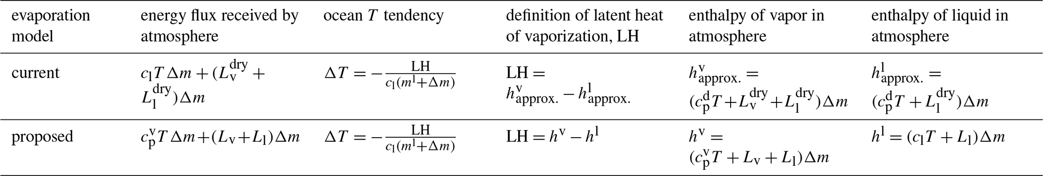
In both the current (Eq. 3) and the proposed (Eq. 6) models, the ocean temperature tendency is proportional to the latent heat of vaporization, defined as the difference in enthalpy between vapor and liquid forms of same mass Δm. However, in the current model, these enthalpies are defined using dry-air heat capacity ($c_{\mathrm{p}}^{\mathrm{d}}$), while the proposed model uses species-appropriate heat capacities. These conceptual differences are summarized in Table 1. We observe from comparing the current and the proposed design that during evaporation, in the current model, the atmosphere receives and the ocean loses more energy than in the proposed model. Later in Sect. 4 we will show that condensation triggers an opposite behavior in the energy deficit/excess in the current model. However, the magnitude of errors (measured as differences between the current model and the model with unapproximated thermodynamics) during condensation are smaller than those during evaporation.

Table 1 Conceptual summary of the current and proposed implementations of evaporation. The table uses general T symbol for temperature.

2.2.4 Bulk methods do not capture energy transfers from water phase changes

Surface stress fluxes, often represented using Monin–Obukhov Similarity Theory (MOST), are typically modeled using bulk formulations of the form:

$$F_X=\mathit{\rho }{C}_X(X_z-X_{\text{surf}}),$$

where F_X is a flux of quantity X (temperature, a velocity component, or vapor), ρ is the air density, C_X is a combination of transfer coefficients and bulk expressions, and X_z and X_surf represent the value of the variable X at some reference height, z, and at the surface, respectively (Fairall et al., 1996; Taylor, 2015).

The key point of our work is that while these bulk schemes compute a mass flux of vapor and a heat flux, they do not explicitly model the heat transfers during evaporation. This differs from the treatment in atmospheric physics parametrizations (e.g., evaporated rain), where energy (or enthalpy) conservation due to phase changes is modeled explicitly (Lauritzen et al., 2022; Guba et al., 2024), as well as from the formulation of evaporation we present in Sect. 2.2.2 and 2.2.3.

3 Thermodynamics of phase change and simplified models of ocean-atmosphere water exchanges

In this section, we examine the exchange of water between the ocean and atmosphere in more detail. The full process of converting atmospheric water vapor into oceanic liquid via precipitation is referred to as condensation. Condensation encapsulates a two-part process. The first stage occurs entirely within the atmosphere, where water vapor condenses into droplets – represented by the top/grey portion of the left panel in Fig. 1. The second stage, shown as grey boxes in the right panel, corresponds to the sedimentation or precipitation of these droplets into the ocean.

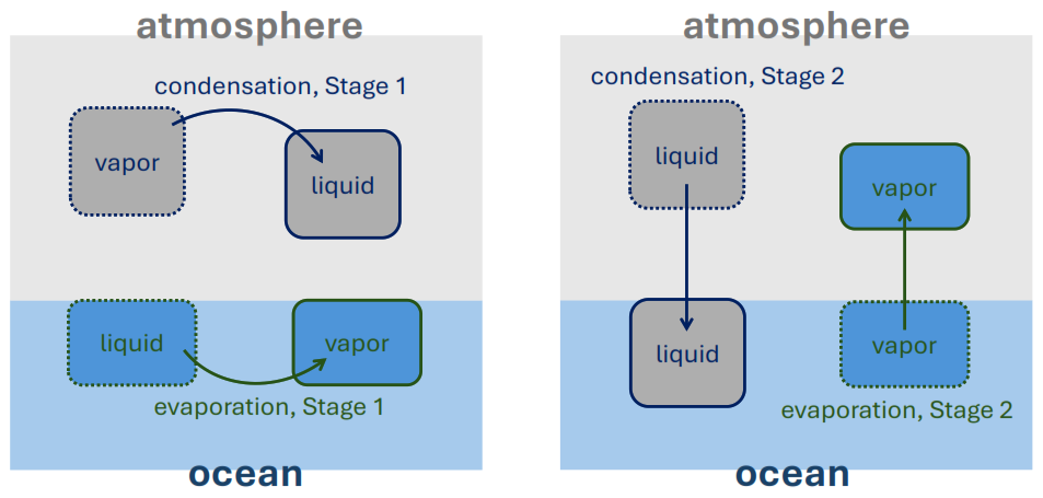
Figure 1 Schematics for the two stages in condensation and evaporation processes: Stage 1 is a phase change within the component, Stage 2 is a transfer of a water species flux to the other component.

Similarly, evaporation is also conceptualized as a two-stage process, illustrated by the blue regions in Fig. 1. When water evaporates from the ocean, it first becomes water vapor within the ocean before subsequently ascending into the atmosphere.

This two-part decomposition of each phase-change process – both from atmosphere to ocean (via precipitation) and from ocean to atmosphere (via evaporation) – is not merely schematic. It is essential for correctly incorporating unapproximated thermodynamics. By distinguishing between the stages, we ensure that the appropriate specific heat capacity is used for the relevant water form (liquid or vapor) at each step.

For example, during Stage 1 of each process, the latent heat exchange occurs within the originating component: in the atmosphere during condensation, and in the ocean during evaporation. This perspective aligns with the discussion of enthalpy and energy partitioning presented earlier in Sect. 2.2.3.

This careful dissection of each leg of the water exchange process directly enables the derivation of unapproximated thermodynamics. It also provides a clear basis for identifying deficiencies in the current E3SM implementation of moist thermodynamics. Within this framework, the time rate of tendencies of atmospheric and oceanic temperature and water mass are formulated as a system of ordinary differential equations in time. This allows us to systematically examine and compare the evolution of the ocean–atmosphere system under both the proposed formulation and the existing E3SM design. We begin with the proposed formulation.

3.1 Unapproximated thermodynamics

In this section we start with deriving equations for tendencies of water mass and temperature in the ocean and the atmosphere. It leads to a system of four coupled algebraic equations. Both components, the atmosphere and the ocean, are modeled as simple dimensionless boxes. The mass variables are defined as follows: $m_{\mathrm{a}}^{\mathrm{v}}$, $m_{\mathrm{a}}^{\mathrm{l}}$, $m_{\mathrm{a}}^{\mathrm{d}}$ denote atmospheric water vapor, liquid, and dry air, respectively, while $m_{\mathrm{o}}^{\mathrm{l}}$ and $m_{\mathrm{o}}^{\mathrm{v}}$ represent oceanic liquid and vapor mass. The temperatures of the atmosphere and the ocean are given by T_a and T_o, respectively. Each variable represents a mean value over a single grid cell or box. The guiding principle for the equations below is conservation of mass and energy after each process (stage). These processes include phase changes (vapor → liquid and liquid → vapor), sedimentation of the atmospheric water liquid into the ocean, and transfer of the evaporated ocean vapor into the atmosphere. Each process updates the initial quantities (unmarked) to new values (denoted with superscript “new”). For example, a mass change in atmospheric water vapor content is written as $\mathrm{\Delta }{m}_{\mathrm{v}}^{\mathrm{a}}:=(m_{\mathrm{a}}^{\mathrm{v}}{)}^{\text{new}}-m_{\mathrm{a}}^{\mathrm{v}}$. For simplicity, we will use such Δ notation as much as possible.

These algebraic equations capture the instantaneous changes in mass and temperature associated with prescribed evaporation and condensation amounts, denoted by ΔV and ΔK, respectively. As these evaporation and condensation rates are assumed to be known, it is useful to convert the algebraic system into time-dependent equations. This leads to a system of ordinary differential equations (ODEs) governing the evolution of atmospheric and oceanic mass and temperature. The derivation of these ODEs is presented in Sect. 3.4.

The total energy is E_atm+E_ocn, where the energy of the atmosphere and ocean is respectively,

$$\begin{array}{}\text{(7)}& \begin{array}{rl}& E_{\text{atm}}=(c_{\mathrm{p}}^{\mathrm{d}}{m}_{\mathrm{a}}^{\mathrm{d}}+c_{\mathrm{p}}^{\mathrm{v}}{m}_{\mathrm{a}}^{\mathrm{v}})T_{\mathrm{a}}+(L_{\mathrm{v}}+L_{\mathrm{l}})m_{\mathrm{a}}^{\mathrm{v}},\\ & E_{\text{ocn}}=c_{\mathrm{l}}{T}_{\mathrm{o}}{m}_{\mathrm{o}}^{\mathrm{l}}+L_{\mathrm{l}}{m}_{\mathrm{o}}.\end{array}\end{array}$$

The first terms in E_atm and E_ocn, involving heat capacities multiplied with temperature are commonly referred to as enthalpies in the literature. In older formulations, enthalpy is frequently defined without the L terms, treating the corresponding energy released or absorbed during phase transitions of water as external inputs. Such an approach complicates energy conservation in a model due to an increased requirement of book-keeping. Therefore, we adhere to definitions of enthalpy that include L terms, like in Thuburn (2017) and Eldred et al. (2022). Sometimes, in this work, we operate with energy defined by the L terms. We may refer to this energy as latent heat internal energy. Let us now consider the required tendencies in the condensation process, before addressing the evaporation.

3.1.1 Condensation

As schematized earlier in the grey portion of Fig. 1a during the first stage in the condensation process, a phase change occurs such that a mass ΔK>0 of water vapor undergoes phase change to become liquid while remaining suspended in the atmosphere. Therefore, the mass balance is

$$\mathrm{\Delta }{m}_{\mathrm{a}}^{\mathrm{v}}=-\mathrm{\Delta }K,\mathrm{\Delta }{m}_{\mathrm{a}}^{\mathrm{l}}=\mathrm{\Delta }K,\mathrm{\Delta }{m}_{\mathrm{o}}^{\mathrm{l}}=\mathrm{0},\mathrm{\Delta }{m}_{\mathrm{o}}^{\mathrm{v}}=\mathrm{0}.$$

Before the phase change, the condensing vapor has specific heat capacity $c_{\mathrm{p}}^{\mathrm{v}}$ and latent heat internal energy L_v+L_l. After the phase change, the resulting liquid has heat capacity c_l and latent energy L_v. Assuming the atmospheric temperature changes from T_a to $T_{\mathrm{a}}^{\text{new}}$, the energy conservation is formulated as:

$$\begin{array}{rl}& \underset{\text{energy of atm. before phase change}}{\underbrace{\left(c_{\mathrm{p}}^{\mathrm{v}}\right(m_{\mathrm{a}}^{\mathrm{v}}+\mathrm{\Delta }K)+c_{\mathrm{p}}^{\mathrm{d}}{m}_{\mathrm{a}}^{\mathrm{d}})T_{\mathrm{a}}+(L_{\mathrm{v}}+L_{\mathrm{l}})(m_{\mathrm{a}}^{\mathrm{v}}+\mathrm{\Delta }K)}}=\\ & \underset{\text{energy of atm. after phase change}}{\underbrace{(c_{\mathrm{p}}^{\mathrm{v}}{m}_{\mathrm{a}}^{\mathrm{v}}+c_{\mathrm{l}}\mathrm{\Delta }K+c_{\mathrm{p}}^{\mathrm{d}}{m}_{\mathrm{a}}^{\mathrm{d}})T_{\mathrm{a}}^{\text{new}}+(L_{\mathrm{v}}+L_{\mathrm{l}})m_{\mathrm{a}}^{\mathrm{v}}+L_{\mathrm{l}}\mathrm{\Delta }K}}.\end{array}$$

Since no change occurs in the ocean during this stage (denoting grey phase during condensation in Fig. 1, the ocean temperature satisfies ΔT_o=0.

In the second stage of the condensation process, the newly formed liquid is removed from the atmosphere and deposited into the ocean. The atmosphere temperature T_a does not change during this stage. The necessary changes to T_a accompanying condensation related phase change were already included in first stage. The mass conservation in this state implies:

$$\mathrm{\Delta }{m}_{\mathrm{a}}^{\mathrm{v}}=\mathrm{0},\mathrm{\Delta }{m}_{\mathrm{a}}^{\mathrm{l}}=-\mathrm{\Delta }K,\mathrm{\Delta }{m}_{\mathrm{o}}^{\mathrm{l}}=\mathrm{\Delta }K,\mathrm{\Delta }{m}_{\mathrm{o}}^{\mathrm{v}}=\mathrm{0}.$$

The conservation of energy in the ocean leads to:

$$\begin{array}{rl}& \underset{\text{energy of ocn. before precip.}}{\underbrace{c_{\mathrm{l}}{T}_{\mathrm{o}}{m}_{\mathrm{o}}^{\mathrm{l}}+L_{\mathrm{l}}{m}_{\mathrm{o}}^{\mathrm{l}}}}+\underset{\text{energy of precip.}}{\underbrace{c_{\mathrm{l}}{T}_{\mathrm{a}}^{\text{new}}\mathrm{\Delta }K+L_{\mathrm{l}}\mathrm{\Delta }K}}\\ & =\underset{\text{energy of ocn. after precip.}}{\underbrace{c_{\mathrm{l}}{T}_{\mathrm{o}}^{\text{new}}(m_{\mathrm{o}}+\mathrm{\Delta }K)+L_{\mathrm{l}}(m_{\mathrm{o}}^{\mathrm{l}}+\mathrm{\Delta }K)}}.\end{array}$$

Combining both stages and eliminating $m_{\mathrm{a}}^{\mathrm{l}}$ and $m_{\mathrm{o}}^{\mathrm{v}}$, we obtain

$$\begin{array}{}\text{(8)}& {\displaystyle }\mathrm{\Delta }{m}_{\mathrm{a}}^{\mathrm{v}}=-\mathrm{\Delta }K\text{(9)}& {\displaystyle }\mathrm{\Delta }{m}_{\mathrm{o}}^{\mathrm{l}}=\mathrm{\Delta }K\text{(10)}& {\displaystyle }\begin{array}{rl}\left(c_{\mathrm{p}}^{\mathrm{v}}\right(m_{\mathrm{a}}^{\mathrm{v}}& +\mathrm{\Delta }K)+c_{\mathrm{p}}^{\mathrm{d}}{m}_{\mathrm{a}}^{\mathrm{d}})T_{\mathrm{a}}+(L_{\mathrm{v}}+L_{\mathrm{l}})(m_{\mathrm{a}}^{\mathrm{v}}+\mathrm{\Delta }K)\\ & =(c_{\mathrm{p}}^{\mathrm{v}}{m}_{\mathrm{a}}^{\mathrm{v}}+c_{\mathrm{l}}\mathrm{\Delta }K+c_{\mathrm{p}}^{\mathrm{d}}{m}_{\mathrm{a}}^{\mathrm{d}})T_{\mathrm{a}}^{\text{new}}+(L_{\mathrm{v}}\\ & +L_{\mathrm{l}})m_{\mathrm{a}}^{\mathrm{v}}+L_{\mathrm{l}}\mathrm{\Delta }K\end{array}\text{(11)}& {\displaystyle }\begin{array}{rl}{c}_{\mathrm{l}}{m}_{\mathrm{o}}^{\mathrm{l}}{T}_{\mathrm{o}}& +L_{\mathrm{l}}{m}_{\mathrm{o}}^{\mathrm{l}}+c_{\mathrm{l}}{T}_{\mathrm{a}}^{\text{new}}\mathrm{\Delta }K+L_{\mathrm{l}}\mathrm{\Delta }K\\ & =c_{\mathrm{l}}{T}_{\mathrm{o}}^{\text{new}}(m_{\mathrm{o}}^{\mathrm{l}}+\mathrm{\Delta }K)+L_{\mathrm{l}}(m_{\mathrm{o}}^{\mathrm{l}}+\mathrm{\Delta }K)\end{array}\end{array}$$

Converting these algebraic equations into ODEs involves additional assumptions, which we discuss later in Sect. 3.4.1.

3.1.2 Evaporation

The required mass and temperature tendencies of the ocean and atmosphere during evaporation follow a derivation closely analogous to that presented above for condensation. This is detailed in the current subsection. The first stage is the phase change of mass ΔV>0 of oceanic liquid water into vapor, while it remains in the ocean. This representation is essential to correctly model ocean cooling due to latent heat loss. Mass conservation is given by

$$\mathrm{\Delta }{m}_{\mathrm{a}}^{\mathrm{v}}=\mathrm{0},\mathrm{\Delta }{m}_{\mathrm{a}}^{\mathrm{l}}=\mathrm{0},\mathrm{\Delta }{m}_{\mathrm{o}}^{\mathrm{l}}=-\mathrm{\Delta }V,\mathrm{\Delta }{m}_{\mathrm{o}}^{\mathrm{v}}=\mathrm{\Delta }V.$$

Initially, the evaporating liquid has specific heat capacity c_l and latent heat internal energy defined by L_l. After the phase change following evaporation these change to $c_{\mathrm{p}}^{\mathrm{v}}$ and L_v+L_l. The energy conservation for this phase change in the ocean is given by

$$\begin{array}{}\text{(12)}& \begin{array}{rl}& \underset{\text{energy of ocn. before phase change}}{\underbrace{c_{\mathrm{l}}{T}_{\mathrm{o}}(m_{\mathrm{o}}^{\mathrm{l}}+\mathrm{\Delta }V)+L_{\mathrm{l}}(m_{\mathrm{o}}^{\mathrm{l}}+\mathrm{\Delta }V)}}\\ & =\underset{\text{energy of ocn. after phase change}}{\underbrace{(c_{\mathrm{l}}{m}_{\mathrm{o}}^{\mathrm{l}}+c_{\mathrm{p}}^{\mathrm{v}}\mathrm{\Delta }V)T_{\mathrm{o}}^{\text{new}}+L_{\mathrm{l}}{m}_{\mathrm{o}}^{\mathrm{l}}+(L_{\mathrm{v}}+L_{\mathrm{l}})\mathrm{\Delta }V}}.\end{array}\end{array}$$

In the second stage, the vapor leaves the ocean and becomes a part of the atmosphere, following a mass conservation given by

$$\mathrm{\Delta }{m}_{\mathrm{a}}^{\mathrm{v}}=\mathrm{\Delta }V,\mathrm{\Delta }{m}_{\mathrm{a}}^{\mathrm{l}}=\mathrm{0},\mathrm{\Delta }{m}_{\mathrm{o}}^{\mathrm{l}}=\mathrm{0},\mathrm{\Delta }{m}_{\mathrm{o}}^{\mathrm{v}}=-\mathrm{\Delta }V.$$

The energy conservation in the atmosphere is:

$$\begin{array}{rl}& \underset{\text{energy of atm. before evap.}}{\underbrace{(c_{\mathrm{p}}^{\mathrm{d}}{m}_{\mathrm{a}}^{\mathrm{d}}+c_{\mathrm{p}}^{\mathrm{v}}{m}_{\mathrm{a}}^{\mathrm{v}})T_{\mathrm{a}}+(L_{\mathrm{v}}+L_{\mathrm{l}})m_{\mathrm{a}}^{\mathrm{v}}}}\\ & +\underset{\text{energy of evap. flux}}{\underbrace{c_{\mathrm{p}}^{\mathrm{v}}{T}_{\mathrm{o}}^{\text{new}}\mathrm{\Delta }V+(L_{\mathrm{v}}+L_{\mathrm{l}})\mathrm{\Delta }V}}\\ & =\underset{\text{energy of atm. after evap.}}{\underbrace{(c_{\mathrm{p}}^{\mathrm{d}}{m}_{\mathrm{a}}^{\mathrm{d}}+c_{\mathrm{p}}^{\mathrm{v}}{m}_{\mathrm{a}}^{\mathrm{v}}+c_{\mathrm{p}}^{\mathrm{v}}\mathrm{\Delta }V)T_{\mathrm{a}}^{\text{new}}+(L_{\mathrm{v}}+L_{\mathrm{l}})(m_{\mathrm{a}}^{\mathrm{v}}+\mathrm{\Delta }V)}}.\end{array}$$

Combining both stages, we obtain

$$\begin{array}{}\text{(13)}& {\displaystyle }\mathrm{\Delta }{m}_{\mathrm{a}}^{\mathrm{v}}=\mathrm{\Delta }V,\text{(14)}& {\displaystyle }\mathrm{\Delta }{m}_{\mathrm{o}}^{\mathrm{l}}=-\mathrm{\Delta }V,\text{(15)}& {\displaystyle }\begin{array}{rl}{c}_{\mathrm{l}}{T}_{\mathrm{o}}(m_{\mathrm{o}}^{\mathrm{l}}+\mathrm{\Delta }V)& +L_{\mathrm{l}}(m_{\mathrm{o}}^{\mathrm{l}}+\mathrm{\Delta }V)\\ & =(c_{\mathrm{l}}{m}_{\mathrm{o}}^{\mathrm{l}}+c_{\mathrm{p}}^{\mathrm{v}}\mathrm{\Delta }V)T_{\mathrm{o}}^{\text{new}}+L_{\mathrm{l}}{m}_{\mathrm{o}}^{\mathrm{l}}\\ & +(L_{\mathrm{v}}+L_{\mathrm{l}})\mathrm{\Delta }V,\end{array}\text{(16)}& {\displaystyle }\begin{array}{rl}(c_{\mathrm{p}}^{\mathrm{d}}{m}_{\mathrm{a}}^{\mathrm{d}}& +c_{\mathrm{p}}^{\mathrm{v}}{m}_{\mathrm{a}}^{\mathrm{v}})T_{\mathrm{a}}+c_{\mathrm{p}}^{\mathrm{v}}{T}_{\mathrm{o}}^{\text{new}}\mathrm{\Delta }V+(L_{\mathrm{v}}+L_{\mathrm{l}}\left)\right(m_{\mathrm{a}}^{\mathrm{v}}+\mathrm{\Delta }V)\\ & =(c_{\mathrm{p}}^{\mathrm{d}}{m}_{\mathrm{a}}^{\mathrm{d}}+c_{\mathrm{p}}^{\mathrm{v}}{m}_{\mathrm{a}}^{\mathrm{v}}+c_{\mathrm{p}}^{\mathrm{v}}\mathrm{\Delta }V)T_{\mathrm{a}}^{\text{new}}\\ & +(L_{\mathrm{v}}+L_{\mathrm{l}})(m_{\mathrm{a}}^{\mathrm{v}}+\mathrm{\Delta }V).\end{array}\end{array}$$

3.2 Current E3SM implementation

While the E3SM surface exchange thermodynamics were likely not derived in the manner presented here, we reinterpret them using the same framework applied to the unapproximated formulation in the previous section. Here, both evaporation and condensation processes require additional steps that represent pressure adjustment, its energy fixer, and the IEFLX energy fixer previously discussed in Sect. 2.2.2.

In this formulation, the total atmospheric energy differs from that in the unapproximated case, Eq. (7), but the ocean energy remains the same:

$$\begin{array}{}\text{(17)}& \begin{array}{rl}& E_{\text{atm}}=c_{\mathrm{p}}^{\mathrm{d}}(m_{\mathrm{a}}^{\mathrm{d}}+m_{\mathrm{a}}^{\mathrm{v}})T_{\mathrm{a}}+(L_{\mathrm{v}}^{\text{dry}}+L_{\mathrm{l}}^{\text{dry}})m_{\mathrm{a}}^{\mathrm{v}},\\ & E_{\text{ocn}}=c_{\mathrm{l}}{T}_{\mathrm{o}}{m}_{\mathrm{o}}^{\mathrm{l}}+L_{\mathrm{l}}^{\text{dry}}{m}_{\mathrm{o}}.\end{array}\end{array}$$

The difference in atmospheric energy arises from the use of the dry-air specific heat capacity, $c_{\mathrm{p}}^{\mathrm{d}}$, being applied to the atmospheric vapor mass $m_{\mathrm{a}}^{\mathrm{v}}$, instead of the vapor-specific heat capacity $c_{\mathrm{p}}^{\mathrm{v}}$, used previously in Eq. (7). Such discrepancies in specific heat capacities constitute one of the primary sources of divergence between the unapproximated formulation and the current E3SM design. As we will demonstrate in Sect. 4, these are not merely minor quantitative errors – they result in significant qualitative differences in the (simplified) system's behavior.

3.2.1 Condensation

Since in E3SM energy flux of precipitation is not modeled explicitly, it is represented instead by a few processes, as described below. To clearly explain the mechanism of precipitation, in this section we need to operate with one more time index. Besides T_a and $T_{\mathrm{a}}^{\text{new}}$, we introduce intermediate $T_{\mathrm{a}}^{\text{new'}}$.

The first stage in the condensation process remains structurally the same as in the unapproximated case of the previous section, but now with heat capacities of the dry air for water forms in the atmosphere. The mass conservation constitutes

$$\mathrm{\Delta }{m}_{\mathrm{a}}^{\mathrm{v}}=-\mathrm{\Delta }K,\mathrm{\Delta }{m}_{\mathrm{a}}^{\mathrm{l}}=\mathrm{\Delta }K,\mathrm{\Delta }{m}_{\mathrm{o}}^{\mathrm{l}}=\mathrm{0},\mathrm{\Delta }{m}_{\mathrm{o}}^{\mathrm{v}}=\mathrm{0},$$

and the energy conservation during the phase change within the atmosphere is

$$\begin{array}{}\text{(18)}& \begin{array}{rl}& \underset{\text{energy of atm. before phase change}}{\underbrace{c_{\mathrm{p}}^{\mathrm{d}}(m_{\mathrm{a}}^{\mathrm{v}}+m_{\mathrm{a}}^{\mathrm{d}}+\mathrm{\Delta }K)T_{\mathrm{a}}+(L_{\mathrm{v}}^{\text{dry}}+L_{\mathrm{l}}^{\text{dry}})(m_{\mathrm{a}}^{\mathrm{v}}+\mathrm{\Delta }K)}}\\ & =\underset{\text{energy of atm. after phase change}}{\underbrace{c_{\mathrm{p}}^{\mathrm{d}}(m_{\mathrm{a}}^{\mathrm{v}}+m_{\mathrm{a}}^{\mathrm{d}}+\mathrm{\Delta }K)T_{\mathrm{a}}^{\text{new'}}+(L_{\mathrm{v}}^{\text{dry}}+L_{\mathrm{l}}^{\text{dry}})m_{\mathrm{a}}^{\mathrm{v}}+L_{\mathrm{l}}^{\text{dry}}\mathrm{\Delta }K}}.\end{array}\end{array}$$

In the unapproximated case, the sedimentation, included in the second stage of condensation process, did not alter the atmospheric temperature T_a, because the energy flux associated with the precipitating mass ΔK was matched between the ocean and the atmosphere. In E3SM, however, the vapor-to-liquid transition followed by sedimentation is not modeled with consistent energy (or enthalpy) fluxes.

Specifically, in EAM, the energy associated with mass ΔK during sedimentation is given by $L_{\mathrm{l}}^{\text{dry}}\mathrm{\Delta }K$ and $E_{\mathrm{1}}=c_{\mathrm{p}}^{\mathrm{d}}{T}_{\mathrm{a}}^{\text{new'}}\mathrm{\Delta }K$. As described by Neale et al. (2012) and Lauritzen et al. (2022), during the pressure adjustment process, energy E₁ is removed from the atmosphere, but then restored by the dynamical core energy fixer (Lauritzen et al., 2022), ensuring energy conservation in the pressure adjustment process. As a result, the net outgoing energy flux from the atmosphere into the ocean is only $L_{\mathrm{l}}^{\text{dry}}\mathrm{\Delta }K$.

This is further corrected by IEFLX energy fixer, which removes energy $E_{\mathrm{2}}=c_{\mathrm{l}}{T}_{\mathrm{a}}^{\text{new}}\mathrm{\Delta }K$ (or E₂=c_lT_aΔK as temperature ambiguity in such terms is discussed later in Sect. 3.4.1) from the atmosphere via temperature globally. This action restores the correct outgoing energy flux of precipitation to value $E_{\mathrm{2}}+L_{\mathrm{l}}^{\text{dry}}\mathrm{\Delta }K$, which is taken up by the ocean. In our simple box model, after incorporating the net energy transfers, the conservation of energy in the atmosphere and the ocean during the precipitation/sedimentation, i.e., the second stage of condensation process is given by

$$\begin{array}{}\text{(19)}& {\displaystyle }\begin{array}{rl}& \underset{\text{energy of atm. before precip.}}{\underbrace{c_{\mathrm{p}}^{\mathrm{d}}(m_{\mathrm{a}}^{\mathrm{v}}+m_{\mathrm{a}}^{\mathrm{d}}+\mathrm{\Delta }K)T_{\mathrm{a}}^{\text{new'}}+(L_{\mathrm{v}}^{\text{dry}}+L_{\mathrm{l}}^{\text{dry}})m_{\mathrm{a}}^{\mathrm{v}}+L_{\mathrm{l}}^{\text{dry}}\mathrm{\Delta }K}}\\ & =\underset{\text{energy of atm. after precip.}}{\underbrace{c_{\mathrm{p}}^{\mathrm{d}}(m_{\mathrm{a}}^{\mathrm{v}}+m_{\mathrm{a}}^{\mathrm{d}})T_{\mathrm{a}}^{\text{new}}+(L_{\mathrm{v}}^{\text{dry}}+L_{\mathrm{l}}^{\text{dry}})m_{\mathrm{a}}^{\mathrm{v}}}}+\underset{\text{energy of precip.}}{\underbrace{E_{\mathrm{2}}+L_{\mathrm{l}}^{\text{dry}}\mathrm{\Delta }K}}\end{array}\text{(20)}& {\displaystyle }\begin{array}{rl}& \underset{\text{energy of ocn. before precip.}}{\underbrace{c_{\mathrm{l}}{T}_{\mathrm{o}}{m}_{\mathrm{o}}^{\mathrm{l}}+L_{\mathrm{l}}^{\text{dry}}{m}_{\mathrm{o}}^{\mathrm{l}}}}+\underset{\text{energy of precip.}}{\underbrace{E_{\mathrm{2}}+L_{\mathrm{l}}^{\text{dry}}\mathrm{\Delta }K}}\\ & =\underset{\text{energy of ocn. after precip.}}{\underbrace{c_{\mathrm{l}}{T}_{\mathrm{o}}^{\text{new}}(m_{\mathrm{o}}^{\mathrm{l}}+\mathrm{\Delta }K)+L_{\mathrm{l}}^{\text{dry}}(m_{\mathrm{o}}^{\mathrm{l}}+\mathrm{\Delta }K)}}\end{array}\end{array}$$

We re-derive Eqs. (18) and (19) as one equation:

$$\begin{array}{rl}& \underset{\text{energy of atm. before precip.}}{\underbrace{c_{\mathrm{p}}^{\mathrm{d}}(m_{\mathrm{a}}^{\mathrm{d}}+m_{\mathrm{a}}^{\mathrm{v}}+\mathrm{\Delta }K)T_{\mathrm{a}}+(L_{\mathrm{l}}^{\text{dry}}+L_{\mathrm{v}}^{\text{dry}})(m_{\mathrm{a}}^{\mathrm{v}}+\mathrm{\Delta }K)}}\\ & =\underset{\text{energy of atm. after precip.}}{\underbrace{c_{\mathrm{p}}^{\mathrm{d}}(m_{\mathrm{a}}^{\mathrm{d}}+m_{\mathrm{a}}^{\mathrm{v}})T_{\mathrm{a}}^{\text{new}}+(L_{\mathrm{v}}^{\text{dry}}+L_{\mathrm{l}}^{\text{dry}})m_{\mathrm{a}}^{\mathrm{v}}}}\\ & +\underset{\text{energy of precip.}}{\underbrace{c_{\mathrm{l}}{T}_{\mathrm{a}}^{\text{new}}\mathrm{\Delta }K+L_{\mathrm{l}}^{\text{dry}}\mathrm{\Delta }K}}\end{array}$$

Similar to the unapproximated case, combining both stages, we obtain

$$\begin{array}{}\text{(21)}& {\displaystyle }\mathrm{\Delta }{m}_{\mathrm{a}}^{\mathrm{v}}=-\mathrm{\Delta }K\text{(22)}& {\displaystyle }\mathrm{\Delta }{m}_{\mathrm{o}}^{\mathrm{l}}=\mathrm{\Delta }K\text{(23)}& {\displaystyle }\begin{array}{rl}{c}_{\mathrm{p}}^{\mathrm{d}}(m_{\mathrm{a}}^{\mathrm{d}}& +m_{\mathrm{a}}^{\mathrm{v}}+\mathrm{\Delta }K)T_{\mathrm{a}}+(L_{\mathrm{l}}^{\text{dry}}+L_{\mathrm{v}}^{\text{dry}}\left)\right(m_{\mathrm{a}}^{\mathrm{v}}+\mathrm{\Delta }K)\\ & =c_{\mathrm{p}}^{\mathrm{d}}(m_{\mathrm{a}}^{\mathrm{d}}+m_{\mathrm{a}}^{\mathrm{v}})T_{\mathrm{a}}^{\text{new}}+(L_{\mathrm{v}}^{\text{dry}}+L_{\mathrm{l}}^{\text{dry}})m_{\mathrm{a}}^{\mathrm{v}}\\ & +c_{\mathrm{l}}{T}_{\mathrm{a}}^{\text{new}}\mathrm{\Delta }K+L_{\mathrm{l}}^{\text{dry}}\mathrm{\Delta }K\end{array}\text{(24)}& {\displaystyle }\begin{array}{rl}{c}_{\mathrm{l}}(T_{\mathrm{o}}{m}_{\mathrm{o}}^{\mathrm{l}}& +T_{\mathrm{a}}^{\text{new}}\mathrm{\Delta }K)+L_{\mathrm{l}}^{\text{dry}}(m_{\mathrm{o}}^{\mathrm{l}}+\mathrm{\Delta }K)\\ & =c_{\mathrm{l}}{T}_{\mathrm{o}}^{\text{new}}(m_{\mathrm{o}}^{\mathrm{l}}+\mathrm{\Delta }K)+L_{\mathrm{l}}^{\text{dry}}(m_{\mathrm{o}}^{\mathrm{l}}+\mathrm{\Delta }K)\end{array}\end{array}$$

3.2.2 Evaporation

In the current E3SM design, the first stage of the evaporation process incorporating the phase change from liquid to evaporated state within the ocean is implemented via a temperature tendency directly proportional to latent energy of vaporization:

$$\mathrm{\Delta }{T}_{\mathrm{o}}=-{\displaystyle \frac{L_{\mathrm{v}}^{\text{dry}}\mathrm{\Delta }V}{c_{\mathrm{l}}(m_{\mathrm{o}}^{\mathrm{l}}+\mathrm{\Delta }V)}}.$$

This implies the following energy balance equation in the ocean during the phase change process (first stage):

$$\begin{array}{}\text{(25)}& \begin{array}{rl}& \underset{\text{energy of ocn. before phase change}}{\underbrace{c_{\mathrm{l}}{T}_{\mathrm{o}}{m}_{\mathrm{o}}^{\mathrm{l}}+c_{\mathrm{l}}{T}_{\mathrm{o}}\mathrm{\Delta }V+L_{\mathrm{l}}^{\text{dry}}(m_{\mathrm{o}}^{\mathrm{l}}+\mathrm{\Delta }V)}}\\ & =\underset{\text{energy of ocn. after phase change}}{\underbrace{(c_{\mathrm{l}}{m}_{\mathrm{o}}^{\mathrm{l}}+c_{\mathrm{l}}\mathrm{\Delta }V)T_{\mathrm{o}}^{\text{new}}+L_{\mathrm{l}}^{\text{dry}}{m}_{\mathrm{o}}^{\mathrm{l}}+(L_{\mathrm{v}}^{\text{dry}}+L_{\mathrm{l}}^{\text{dry}})\mathrm{\Delta }V}}.\end{array}\end{array}$$

The difference from the unapproximated case (compare Eq. 25 with Eq. 12) lies in the use of c_l (liquid) heat capacity instead of more appropriate $c_{\mathrm{p}}^{\mathrm{v}}$ (vapor) for the evaporated mass.

In the second stage, vapor leaves the ocean and becomes a part of the atmosphere. As with condensation, the pressure adjustment and the dynamical core energy fixer ensure no net atmospheric energy change from this part of the process except for the L term $(L_{\mathrm{v}}^{\text{dry}}+L_{\mathrm{l}}^{\text{dry}})\mathrm{\Delta }V$. The full energy of the incoming vapor mass into the atmosphere is thus corrected with IEFLX term $E_{\mathrm{3}}=c_{\mathrm{l}}{T}_{\mathrm{o}}^{\text{new}}\mathrm{\Delta }V$. This leads to the following equation for the conservation of energy in the atmosphere:

$$\begin{array}{rl}& \underset{\text{energy of atm. before evap. flux}}{\underbrace{c_{\mathrm{p}}^{\mathrm{d}}(m_{\mathrm{a}}^{\mathrm{d}}+m_{\mathrm{a}}^{\mathrm{v}})T_{\mathrm{a}}+(L_{\mathrm{v}}^{\text{dry}}+L_{\mathrm{l}}^{\text{dry}})m_{\mathrm{a}}^{\mathrm{v}}}}\\ & +\underset{\text{energy of evap. flux}}{\underbrace{E_{\mathrm{3}}+(L_{\mathrm{v}}^{\text{dry}}+L_{\mathrm{l}}^{\text{dry}})\mathrm{\Delta }V}}\\ & =\underset{\text{energy of atm. after evap. flux}}{\underbrace{c_{\mathrm{p}}^{\mathrm{d}}(m_{\mathrm{a}}^{\mathrm{d}}+m_{\mathrm{a}}^{\mathrm{v}}+\mathrm{\Delta }V)T_{\mathrm{a}}^{\text{new}}+(L_{\mathrm{v}}^{\text{dry}}+L_{\mathrm{l}}^{\text{dry}})(m_{\mathrm{a}}^{\mathrm{v}}+\mathrm{\Delta }V)}}.\end{array}$$

Unlike condensation, no additional tendency is applied to T_o in the second stage, since the ocean has already lost energy flux $E_{\mathrm{3}}+(L_{\mathrm{v}}^{\text{dry}}+L_{\mathrm{l}}^{\text{dry}})\mathrm{\Delta }V=c_{\mathrm{l}}{T}_{\mathrm{o}}^{\text{new}}\mathrm{\Delta }V+(L_{\mathrm{v}}^{\text{dry}}+L_{\mathrm{l}}^{\text{dry}})\mathrm{\Delta }V$ represented in Eq. (25).

As before, combining the two states, the equations comprising evaporation in E3SM are

$$\begin{array}{}\text{(26)}& {\displaystyle }\mathrm{\Delta }{m}_{\mathrm{a}}^{\mathrm{v}}=\mathrm{\Delta }V,\text{(27)}& {\displaystyle }\mathrm{\Delta }{m}_{\mathrm{o}}^{\mathrm{l}}=-\mathrm{\Delta }V,\text{(28)}& {\displaystyle }\begin{array}{rl}{c}_{\mathrm{l}}{T}_{\mathrm{o}}{m}_{\mathrm{l}}& +c_{\mathrm{l}}{T}_{\mathrm{o}}\mathrm{\Delta }V+L_{\mathrm{l}}^{\text{dry}}(m_{\mathrm{l}}+\mathrm{\Delta }V)\\ & =(c_{\mathrm{l}}{m}_{\mathrm{l}}+c_{\mathrm{l}}\mathrm{\Delta }V)T_{\mathrm{o}}^{\text{new}}+L_{\mathrm{l}}^{\text{dry}}(m_{\mathrm{l}}+\mathrm{\Delta }V)\\ & +L_{\mathrm{v}}^{\text{dry}}\mathrm{\Delta }V,\end{array}\text{(29)}& {\displaystyle }\begin{array}{rl}& c_{\mathrm{p}}^{\mathrm{d}}(m_{\mathrm{a}}^{\mathrm{d}}+m_{\mathrm{a}}^{\mathrm{v}})T_{\mathrm{a}}+(L_{\mathrm{v}}^{\text{dry}}+L_{\mathrm{l}}^{\text{dry}})m_{\mathrm{a}}^{\mathrm{v}}+c_{\mathrm{l}}{T}_{\mathrm{o}}^{\text{new}}\mathrm{\Delta }V\\ & +(L_{\mathrm{v}}^{\text{dry}}+L_{\mathrm{l}}^{\text{dry}})\mathrm{\Delta }V=c_{\mathrm{p}}^{\mathrm{d}}(m_{\mathrm{a}}^{\mathrm{d}}+m_{\mathrm{a}}^{\mathrm{v}}+\mathrm{\Delta }V)T_{\mathrm{a}}^{\text{new}}\\ & +(L_{\mathrm{v}}^{\text{dry}}+L_{\mathrm{l}}^{\text{dry}})(m_{\mathrm{a}}^{\mathrm{v}}+\mathrm{\Delta }V).\end{array}\end{array}$$

The framework presented in this section follows the E3SM formulation, with one box representing the atmosphere and one for the ocean. In this simplified setting – where the distinction between local and global behavior is blurred – the various energy fixers can be interpreted as acting “locally” to each grid cell (just one in our simplified box model). Local energy fixers are known to be detrimental to model fidelity and predictive accuracy (Harrop et al., 2022). In fact, it may be preferable to relax strict energy conservation altogether if globally consistent fixers cannot be applied. Motivated by this, we introduce an alternative model in the next section: an E3SM-like formulation that forgoes net energy conservation.

3.3 Model with E3SM-like behavior (no local fixers)

The systems described by Eqs. (8)–(11), (13)–(16) (for the unapproximated case) and Eqs. (21)–(24), (26)–(29) (for the current E3SM design) represent significant simplifications relative to the full complexity of E3SM. In the actual E3SM implementation, IEFLX terms, partially responsible for the nonphysical behavior observed in the simplified version of current model discussed later in Sect. 4, are applied as global fixers. These are implemented as globally integrated energy corrections that result in the same temperature tendency at each horizontal grid cell at each vertical model level. Importantly, because the evaporation and precipitation fluxes are approximately globally balanced in E3SM, the magnitude of these temperature corrections (due to both IEFLX and the dynamical core energy fixer) is relatively small at each grid point.

Since the fixers in the actual E3SM simulations lead to small temperature tendencies, we modify the Eqs. (23)–(24), (28)–(29) for current E3SM implementation and remove the effect of the IEFLX and the dynamical core fixer. This model maintains the basic thermodynamic structure of E3SM but relaxes net energy conservation. Because the pressure adjustment in E3SM does not modify the atmospheric temperature T_a, there is no temperature tendency from that process. Accordingly, we modify the current model's equations as follows. For condensation, we rewrite Eq. (23) as

$$\begin{array}{rl}{c}_{\mathrm{p}}^{\mathrm{d}}(m_{\mathrm{a}}^{\mathrm{d}}& +m_{\mathrm{a}}^{\mathrm{v}}+\mathrm{\Delta }K)T_{\mathrm{a}}+(L_{\mathrm{l}}^{\text{dry}}+L_{\mathrm{v}}^{\text{dry}}\left)\right(m_{\mathrm{a}}^{\mathrm{v}}+\mathrm{\Delta }K)\\ & =c_{\mathrm{p}}^{\mathrm{d}}(m_{\mathrm{a}}^{\mathrm{d}}+m_{\mathrm{a}}^{\mathrm{v}})T_{\mathrm{a}}^{\text{new}}+(L_{\mathrm{v}}^{\text{dry}}+L_{\mathrm{l}}^{\text{dry}})m_{\mathrm{a}}^{\mathrm{v}}+c_{\mathrm{p}}^{\mathrm{d}}{T}_{\mathrm{a}}^{\text{new}}\mathrm{\Delta }K\\ & +L_{\mathrm{l}}^{\text{dry}}\mathrm{\Delta }K.\end{array}$$

For evaporation, the current design of E3SM implies that there is no temperature tendency for T_a due to the incoming evaporative flux. Thus, there is no atmospheric energy equation analogous to Eq. (29) and no corresponding correction to T_a arising from ΔV.

3.4 From tendency (algebraic) equations to time derivatives (ODEs)

3.4.1 Considerations

Now we reformulate the systems of algebraic equations representing the tendencies of oceanic and atmospheric mass and temperature from above as systems of ordinary differential equations representing the time rate of these tendencies. We begin with the unapproximated condensation model defined by Eqs. (8)–(11) and outline the assumptions used in this reformulation in detail.

Consider Eq. (8). Introducing a finite time step Δt over which the change $\mathrm{\Delta }{m}_{\mathrm{a}}^{\mathrm{v}}$ occurs, we arrive at:

$$\mathrm{\Delta }{m}_{\mathrm{a}}^{\mathrm{v}}=-\mathrm{\Delta }K\Rightarrow {\displaystyle \frac{\mathrm{\Delta }{m}_{\mathrm{a}}^{\mathrm{v}}}{\mathrm{\Delta }t}}=-{\displaystyle \frac{\mathrm{\Delta }K}{\mathrm{\Delta }t}}\Rightarrow {\displaystyle \frac{\mathrm{d}{m}_{\mathrm{a}}^{\mathrm{v}}}{\mathrm{d}t}}=-{\displaystyle \frac{\mathrm{d}K}{\mathrm{d}t}},$$

where $\frac{\mathrm{d}K}{\mathrm{d}t}$ is the condensation rate, to be defined later. Now consider the energy balance from Eq. (10), repeated below:

$$\begin{array}{rl}& \left(c_{\mathrm{p}}^{\mathrm{v}}\right(m_{\mathrm{a}}^{\mathrm{v}}+\mathrm{\Delta }K)+c_{\mathrm{p}}^{\mathrm{d}}{m}_{\mathrm{a}}^{\mathrm{d}})T_{\mathrm{a}}+(L_{\mathrm{v}}+L_{\mathrm{l}})(m_{\mathrm{a}}^{\mathrm{v}}+\mathrm{\Delta }K)\\ & =(c_{\mathrm{p}}^{\mathrm{v}}{m}_{\mathrm{a}}^{\mathrm{v}}+c_{\mathrm{l}}\mathrm{\Delta }K+c_{\mathrm{p}}^{\mathrm{d}}{m}_{\mathrm{a}}^{\mathrm{d}})T_{\mathrm{a}}^{\text{new}}+(L_{\mathrm{v}}+L_{\mathrm{l}})m_{\mathrm{a}}^{\mathrm{v}}+L_{\mathrm{l}}\mathrm{\Delta }K.\end{array}$$

To the leading order in ΔK we can express the atmospheric temperature tendency as:

$$\begin{array}{}\text{(30)}& \begin{array}{rl}& T_{\mathrm{a}}^{\text{new}}-T_{\mathrm{a}}=\mathrm{\Delta }{T}_{\mathrm{a}}={\displaystyle \frac{c_{\mathrm{p}}^{\mathrm{v}}{T}_{\mathrm{a}}-c_{\mathrm{l}}{T}_{\mathrm{a}}+L_{\mathrm{v}}}{c_{\mathrm{p}}^{\mathrm{d}}{m}_{\mathrm{a}}^{\mathrm{d}}+c_{\mathrm{p}}^{\mathrm{v}}{m}_{\mathrm{a}}^{\mathrm{v}}+c_{\mathrm{l}}\mathrm{\Delta }K}}\mathrm{\Delta }K\\ & ={\displaystyle \frac{c_{\mathrm{p}}^{\mathrm{v}}{T}_{\mathrm{a}}-c_{\mathrm{l}}{T}_{\mathrm{a}}+L_{\mathrm{v}}}{c_{\mathrm{p}}^{\mathrm{d}}{m}_{\mathrm{a}}^{\mathrm{d}}+c_{\mathrm{p}}^{\mathrm{v}}{m}_{\mathrm{a}}^{\mathrm{v}}}}\mathrm{\Delta }K+O\left(\right(\mathrm{\Delta }K{)}^{\mathrm{2}}).\end{array}\end{array}$$

Dividing this by Δt, taking the limit, Δt→0, and considering only the first order terms in the condensation rate, $\mathrm{d}K/\mathrm{d}t={lim}_{\mathrm{\Delta }t\to \mathrm{0}}(\mathrm{\Delta }K/\mathrm{\Delta }t)$, we obtain the corresponding ODE for atmospheric temperature,

$$\begin{array}{}\text{(31)}& {\displaystyle \frac{\mathrm{d}{T}_{\mathrm{a}}}{\mathrm{d}t}}={\displaystyle \frac{c_{\mathrm{p}}^{\mathrm{v}}{T}_{\mathrm{a}}-c_{\mathrm{l}}{T}_{\mathrm{a}}+L_{\mathrm{v}}}{c_{\mathrm{p}}^{\mathrm{d}}{m}_{\mathrm{a}}^{\mathrm{d}}+c_{\mathrm{p}}^{\mathrm{v}}{m}_{\mathrm{a}}^{\mathrm{v}}}}{\displaystyle \frac{\mathrm{d}K}{\mathrm{d}t}}.\end{array}$$

One could have considered Eq. (10) with term c_lΔKT_a instead of $c_{\mathrm{l}}\mathrm{\Delta }K{T}_{\mathrm{a}}^{\text{new}}$. We claim that the linearity imposed on Eq. (31) with respect to $\frac{\mathrm{d}K}{\mathrm{d}t}$ eliminates such ambiguities: Assume that Eq. (10) contains c_lΔKT_a instead. Then the difference between this new equation and the original is in term $c_{\mathrm{l}}\mathrm{\Delta }K(T_{\mathrm{a}}-T_{\mathrm{a}}^{\text{new}})$. It can be shown that this difference, proportional to ΔK, propagates to Eq. (30) as term proportional to (ΔK)², and is thus eliminated from Eq. (31).

The approach above is applied systematically to all the variables in both condensation and evaporation processes to derive the full set of time-dependent governing equations for our simplified box model. The resulting systems of ODEs are presented in the following three subsections, corresponding to each of the three models: the unapproximated model (labeled as System I for Ideal), the current E3SM implementation (labeled as System A1 for First Approximation), and the E3SM-like model without energy fixers (labeled as System A2 for Second Approximation).

3.4.2 The final ODE system for the ideal case: System I

Analogously to the steps above, we convert the entire algebraic system Eqs. (8)–(11) into the system of ODEs

$$\begin{array}{}\text{(32)}& {\displaystyle \frac{\mathrm{d}{m}_{\mathrm{a}}^{\mathrm{v}}}{\mathrm{d}t}}=-{\displaystyle \frac{\mathrm{d}K}{\mathrm{d}t}},\text{(33)}& {\displaystyle \frac{\mathrm{d}{m}_{\mathrm{o}}^{\mathrm{l}}}{\mathrm{d}t}}={\displaystyle \frac{\mathrm{d}K}{\mathrm{d}t}},\text{(34)}& {\displaystyle \frac{\mathrm{d}{T}_{\mathrm{a}}}{\mathrm{d}t}}={\displaystyle \frac{c_{\mathrm{p}}^{\mathrm{v}}{T}_{\mathrm{a}}-c_{\mathrm{l}}{T}_{\mathrm{a}}+L_{\mathrm{v}}}{c_{\mathrm{p}}^{\mathrm{d}}{m}_{\mathrm{a}}^{\mathrm{d}}+c_{\mathrm{p}}^{\mathrm{v}}{m}_{\mathrm{a}}^{\mathrm{v}}}}{\displaystyle \frac{\mathrm{d}K}{\mathrm{d}t}},\text{(35)}& {\displaystyle \frac{\mathrm{d}{T}_{\mathrm{o}}}{\mathrm{d}t}}={\displaystyle \frac{T_{\mathrm{a}}-T_{\mathrm{o}}}{m_{\mathrm{l}}^o}}{\displaystyle \frac{\mathrm{d}K}{\mathrm{d}t}}\end{array}$$

From the evaporation Eqs. (13)–(16) we similarly obtain:

$$\begin{array}{}\text{(36)}& {\displaystyle \frac{\mathrm{d}{m}_{\mathrm{a}}^{\mathrm{v}}}{\mathrm{d}t}}={\displaystyle \frac{\mathrm{d}V}{\mathrm{d}t}},\text{(37)}& {\displaystyle \frac{\mathrm{d}{m}_{\mathrm{o}}^{\mathrm{l}}}{\mathrm{d}t}}=-{\displaystyle \frac{\mathrm{d}V}{\mathrm{d}t}},\text{(38)}& {\displaystyle \frac{\mathrm{d}{T}_{\mathrm{a}}}{\mathrm{d}t}}={\displaystyle \frac{c_{\mathrm{p}}^{\mathrm{v}}(T_{\mathrm{o}}-T_{\mathrm{a}})}{c_{\mathrm{p}}^{\mathrm{d}}{m}_{\mathrm{a}}^{\mathrm{d}}+c_{\mathrm{p}}^{\mathrm{v}}{m}_{\mathrm{a}}^{\mathrm{v}}}}{\displaystyle \frac{\mathrm{d}V}{\mathrm{d}t}},\text{(39)}& {\displaystyle \frac{\mathrm{d}{T}_{\mathrm{o}}}{\mathrm{d}t}}={\displaystyle \frac{c_{\mathrm{l}}{T}_{\mathrm{o}}-c_{\mathrm{p}}^{\mathrm{v}}{T}_{\mathrm{o}}-L_{\mathrm{v}}}{c_{\mathrm{l}}{m}_{\mathrm{o}}^{\mathrm{l}}}}{\displaystyle \frac{\mathrm{d}V}{\mathrm{d}t}}\end{array}$$

Combining both condensation and evaporation, the full system becomes

$$\begin{array}{}\text{(40)}& {\displaystyle \frac{\mathrm{d}{m}_{\mathrm{a}}^{\mathrm{v}}}{\mathrm{d}t}}=-{\displaystyle \frac{\mathrm{d}K}{\mathrm{d}t}}+{\displaystyle \frac{\mathrm{d}V}{\mathrm{d}t}},\text{(41)}& {\displaystyle \frac{\mathrm{d}{m}_{\mathrm{o}}^{\mathrm{l}}}{\mathrm{d}t}}={\displaystyle \frac{\mathrm{d}K}{\mathrm{d}t}}-{\displaystyle \frac{\mathrm{d}V}{\mathrm{d}t}},\text{(42)}& {\displaystyle \frac{\mathrm{d}{T}_{\mathrm{a}}}{\mathrm{d}t}}={\displaystyle \frac{c_{\mathrm{p}}^{\mathrm{v}}{T}_{\mathrm{a}}-c_{\mathrm{l}}{T}_{\mathrm{a}}+L_{\mathrm{v}}}{c_{\mathrm{p}}^{\mathrm{d}}{m}_{\mathrm{a}}^{\mathrm{d}}+c_{\mathrm{p}}^{\mathrm{v}}{m}_{\mathrm{a}}^{\mathrm{v}}}}{\displaystyle \frac{\mathrm{d}K}{\mathrm{d}t}}+{\displaystyle \frac{c_{\mathrm{p}}^{\mathrm{v}}(T_{\mathrm{o}}-T_{\mathrm{a}})}{c_{\mathrm{p}}^{\mathrm{d}}{m}_{\mathrm{a}}^{\mathrm{d}}+c_{\mathrm{p}}^{\mathrm{v}}{m}_{\mathrm{a}}^{\mathrm{v}}}}{\displaystyle \frac{\mathrm{d}V}{\mathrm{d}t}},\text{(43)}& {\displaystyle \frac{\mathrm{d}{T}_{\mathrm{o}}}{\mathrm{d}t}}={\displaystyle \frac{T_{\mathrm{a}}-T_{\mathrm{o}}}{m_{\mathrm{l}}^o}}{\displaystyle \frac{\mathrm{d}K}{\mathrm{d}t}}+{\displaystyle \frac{c_{\mathrm{l}}{T}_{\mathrm{o}}-c_{\mathrm{p}}^{\mathrm{v}}{T}_{\mathrm{o}}-L_{\mathrm{v}}}{c_{\mathrm{l}}{m}_{\mathrm{o}}^{\mathrm{l}}}}{\displaystyle \frac{\mathrm{d}V}{\mathrm{d}t}}.\end{array}$$

3.4.3 The final ODE system for the current case: System A1

Applying the same procedure to the algebraic systems (21)–(24) and (26)–(29), we obtain

$$\begin{array}{}\text{(44)}& {\displaystyle \frac{\mathrm{d}{m}_{\mathrm{a}}^{\mathrm{v}}}{\mathrm{d}t}}=-{\displaystyle \frac{\mathrm{d}K}{\mathrm{d}t}}+{\displaystyle \frac{\mathrm{d}V}{\mathrm{d}t}},\text{(45)}& {\displaystyle \frac{\mathrm{d}{m}_{\mathrm{o}}^{\mathrm{l}}}{\mathrm{d}t}}={\displaystyle \frac{\mathrm{d}K}{\mathrm{d}t}}-{\displaystyle \frac{\mathrm{d}V}{\mathrm{d}t}},\text{(46)}& {\displaystyle \frac{\mathrm{d}{T}_{\mathrm{a}}}{\mathrm{d}t}}={\displaystyle \frac{c_{\mathrm{p}}^{\mathrm{d}}{T}_{\mathrm{a}}-c_{\mathrm{l}}{T}_{\mathrm{a}}+L_{\mathrm{v}}^{\text{dry}}}{c_{\mathrm{p}}^{\mathrm{d}}(m_{\mathrm{a}}^{\mathrm{d}}+m_{\mathrm{a}}^{\mathrm{v}})}}{\displaystyle \frac{\mathrm{d}K}{\mathrm{d}t}}+{\displaystyle \frac{c_{\mathrm{l}}{T}_{\mathrm{o}}-c_{\mathrm{p}}^{\mathrm{d}}{T}_{\mathrm{a}}}{c_{\mathrm{p}}^{\mathrm{d}}(m_{\mathrm{a}}^{\mathrm{d}}+m_{\mathrm{a}}^{\mathrm{v}})}}{\displaystyle \frac{\mathrm{d}V}{\mathrm{d}t}},\text{(47)}& {\displaystyle \frac{\mathrm{d}{T}_{\mathrm{o}}}{\mathrm{d}t}}={\displaystyle \frac{T_{\mathrm{a}}-T_{\mathrm{o}}}{m_{\mathrm{o}}^{\mathrm{l}}}}{\displaystyle \frac{\mathrm{d}K}{\mathrm{d}t}}-{\displaystyle \frac{L_{\mathrm{v}}^{\text{dry}}}{c_{\mathrm{l}}{m}_{\mathrm{o}}^{\mathrm{l}}}}{\displaystyle \frac{\mathrm{d}V}{\mathrm{d}t}}.\end{array}$$

One can verify that systems (40)–(43) and (44)–(47) are energy-conserving in the sense that $\frac{\mathrm{d}(E_{\text{atm}}+E_{\text{ocn}})}{\mathrm{d}t}=\mathrm{0}$.

3.4.4 The final ODE system for the E3SM-like case: System A2

Here, the energy fixers are omitted, and we obtain:

$$\begin{array}{}\text{(48)}& {\displaystyle \frac{\mathrm{d}{m}_{\mathrm{a}}^{\mathrm{v}}}{\mathrm{d}t}}=-{\displaystyle \frac{\mathrm{d}K}{\mathrm{d}t}}+{\displaystyle \frac{\mathrm{d}V}{\mathrm{d}t}},\text{(49)}& {\displaystyle \frac{\mathrm{d}{m}_{\mathrm{o}}^{\mathrm{l}}}{\mathrm{d}t}}={\displaystyle \frac{\mathrm{d}K}{\mathrm{d}t}}-{\displaystyle \frac{\mathrm{d}V}{\mathrm{d}t}},\text{(50)}& {\displaystyle \frac{\mathrm{d}{T}_{\mathrm{a}}}{\mathrm{d}t}}={\displaystyle \frac{L_{\mathrm{v}}^{\text{dry}}}{c_{\mathrm{p}}^{\mathrm{d}}(m_{\mathrm{a}}^{\mathrm{d}}+m_{\mathrm{a}}^{\mathrm{v}})}}{\displaystyle \frac{\mathrm{d}K}{\mathrm{d}t}},\text{(51)}& {\displaystyle \frac{\mathrm{d}{T}_{\mathrm{o}}}{\mathrm{d}t}}={\displaystyle \frac{T_{\mathrm{a}}-T_{\mathrm{o}}}{m_{\mathrm{o}}^{\mathrm{l}}}}{\displaystyle \frac{\mathrm{d}K}{\mathrm{d}t}}-{\displaystyle \frac{L_{\mathrm{v}}^{\text{dry}}}{c_{\mathrm{l}}{m}_{\mathrm{o}}^{\mathrm{l}}}}{\displaystyle \frac{\mathrm{d}V}{\mathrm{d}t}}.\end{array}$$

Note that this system does not conserve energy (Eq. 17) due to the omission of the IEFLX and dynamical core fixers.

3.4.5 Atmospheric temperature tendency due to evaporation

We draw attention to the $\frac{\mathrm{d}V}{\mathrm{d}t}$ term in $\frac{\mathrm{d}{T}_{\mathrm{a}}}{\mathrm{d}t}$ equations. In the three systems, it appears as

• System I:

  $${\displaystyle \frac{c_{\mathrm{p}}^{\mathrm{v}}(T_{\mathrm{o}}-T_{\mathrm{a}})}{c_{\mathrm{p}}^{\mathrm{d}}{m}_{\mathrm{a}}^{\mathrm{d}}+c_{\mathrm{p}}^{\mathrm{v}}{m}_{\mathrm{a}}^{\mathrm{v}}}}{\displaystyle \frac{\mathrm{d}V}{\mathrm{d}t}},$$

• System A1:

  $${\displaystyle \frac{c_{\mathrm{l}}{T}_{\mathrm{o}}-c_{\mathrm{p}}^{\mathrm{d}}{T}_{\mathrm{a}}}{c_{\mathrm{p}}^{\mathrm{d}}(m_{\mathrm{a}}^{\mathrm{d}}+m_{\mathrm{a}}^{\mathrm{v}})}}{\displaystyle \frac{\mathrm{d}V}{\mathrm{d}t}},$$

• System A2: Zero (no contribution to $\frac{\mathrm{d}{T}_{\mathrm{a}}}{\mathrm{d}t}$ from evaporation).

Therefore, in System I, the temperature tendency depends on the temperature difference at the ocean-atmosphere interface, which is physically reasonable. In contrast, since $c_{\mathrm{l}}\approx \mathrm{4}{c}_{\mathrm{p}}^{\mathrm{d}}$, System A1 yields positive tendency in atmospheric temperature for realistic values of T_a and T_o, regardless of the sign of difference T_o−T_a, which we regard as physically unrealistic. In System A2, the absence of any $\frac{\mathrm{d}{T}_{\mathrm{a}}}{\mathrm{d}t}$ tendency due to evaporation is also implausible. Below in Sect. 4 we show that the physically unrealistic $\frac{\mathrm{d}{T}_{\mathrm{a}}}{\mathrm{d}t}$ term in System A1 contributes to the system's unstable behavior.

3.4.6 Three systems and their relation to E3SM

With the simplified models for thermodynamic exchange at the ocean–atmosphere interface in place – System I (ideal with unapproximated thermodynamics), System A1 (E3SM-like with fixers), and System A2 (E3SM-like without fixers) – we now clarify their correspondence to E3SM and the assumptions involved.

If we consider the whole Earth system to be presented by two boxes, one for the ocean and one for the atmosphere, just like we outlined in Sect. 3.1, then System A1 is an appropriate representation of E3SM, while System A2 is not, since it does not conserve energy. However, E3SM consists of many degrees of freedom, effectively many vertical columns, and in that context, each column's thermodynamic treatment aligns more closely with System A2, before energy fixers are applied.

These energy fixers in E3SM simulations are relatively small in magnitude. Their values can be approximated via c_lT_surf(P−Q) for IEFLX (Golaz et al., 2019) and $c_{\mathrm{p}}^{\mathrm{d}}{T}_{\mathrm{surf}}(P-Q)$ for the dycore fixer (Lauritzen et al., 2022), where P and Q are globally integrated precipitation and evaporation rates, respectively. In time-averaged multi-seasonal runs, P≈Q within about $\mathrm{1}\times {\mathrm{10}}^{-\mathrm{8}}$ kg m⁻² s⁻¹. Thus, an ensemble of system A2 models, each representing a vertical column, is a valid proxy for E3SM as long as global precipitation and evaporation approximately balance. This ensemble would require a small global energy correction of the order $\mathrm{3}\times {\mathrm{10}}^{-\mathrm{3}}$ to $\mathrm{1.2}\times {\mathrm{10}}^{-\mathrm{2}}$ W m⁻².

By contrast, System A1 does not accurately describe E3SM's behavior when modeling multiple columns, as it effectively implements a local energy fixer. Such local fixers have been shown to degrade performance (Harrop et al., 2022). Later in Sect. 4 we demonstrate that there are regimes when System A1 exhibits numerical instabilities. This actually does not indicate similar instabilities in E3SM, as the instabilities can be attributed to energy fixers, which, as explained above, are of small magnitudes in E3SM. However, we find that both System A1 and System A2 are important for our discussion about deficiencies of the approximated thermodynamics in E3SM.

System I, unlike A1 and A2, does not require external assumptions about energy fixers or balance of precipitation and evaporation. It can be used in either the global box model setting or in multi-column settings, and it always conserves energy since that is built into it from the first principles. Furthermore, unlike current design of E3SM, it does not require an implicit requirement of P≈Q.

3.4.7 Evaporation and condensation rates

In all systems, we define the evaporation and condensation rates as

$$\begin{array}{}\text{(52)}& {\displaystyle }\begin{array}{rl}{\displaystyle \frac{\mathrm{d}V}{\mathrm{d}t}}(m_{\mathrm{a}}^{\mathrm{v}},T_{\mathrm{a}})& =C_{\mathrm{h}}\left|u\right|{\displaystyle \frac{\mathrm{1}}{z_{\mathrm{a}}}}max\mathit{\left\{}\right(m_{\mathrm{a}}^{\mathrm{d}}+m_{\mathrm{a}}^{\mathrm{v}}\left)q_{\text{sat}}\right(T_{\mathrm{a}})\\ & -m_{\mathrm{a}}^{\mathrm{v}},\mathrm{0}\mathit{\}},\end{array}\text{(53)}& {\displaystyle \frac{\mathrm{d}K}{\mathrm{d}t}}(m_{\mathrm{a}}^{\mathrm{v}},T_{\mathrm{a}})=\mathit{\lambda }max\mathit{\{}{m}_{\mathrm{a}}^{\mathrm{v}}-(m_{\mathrm{a}}^{\mathrm{d}}+m_{\mathrm{a}}^{\mathrm{v}}\left)q_{\text{sat}}\right(T_{\mathrm{a}}),\mathrm{0}\mathit{\}},\text{(54)}& {\displaystyle }{q}_{\text{sat}}\left(T\right)={\displaystyle \frac{c_{\mathrm{1}}\cdot c_{\mathrm{2}}}{p_{\mathrm{0}}}}\exp \left(-{\displaystyle \frac{L_{\mathrm{v}}^{\text{dry}}}{R_{\mathrm{v}}}}\left({\displaystyle \frac{\mathrm{1}}{T}}-{\displaystyle \frac{\mathrm{1}}{T_{\mathrm{0}}}}\right)\right),\end{array}$$

where the constants are: C_h=0.0011, $\left|u\right|=\mathrm{50.0}$ m s⁻¹, z_a=50.0 m, $\mathit{\lambda }=\mathrm{1}/\mathrm{100}$ s⁻¹, c₁=0.622, c₂=610.78 Pa, p₀=10⁵ Pa, R_v=461 J kg⁻¹ K⁻¹, and T₀=273.16 K. The mass of the dry air in simulations below is fixed to $m_{\mathrm{a}}^{\mathrm{d}}=\mathrm{1000}$ kg and ocean's mass is initialized to 5000 kg in all cases presented in the next section.

In the next section, we use MATLAB’s numerical ODE integration tools to simulate the evolution of atmospheric and oceanic mass and temperature, in order to evaluate the performance of the three models: System I, System A1, and System A2.

Since q_sat is well defined away from T=0, functions (52) and (53) are continuous and Lipschitz-continuous away from T=0 K, ensuring existence and uniqueness of solutions under physically relevant conditions (away from T=0 K).

4 Numerical analysis of Systems I, A1, and A2

In all three models, the rates evaporation and condensation processes depend oppositely on the sign of $(m_{\mathrm{a}}^{\mathrm{v}}+m_{\mathrm{a}}^{\mathrm{d}})q_{\text{sat}}\left(T_{\mathrm{a}}\right)-m_{\mathrm{a}}^{\mathrm{v}}$ (see Eqs. 52 and 53). Therefore, these processes do not occur simultaneously. The steady state condition for vapor-liquid mass and temperature exchange system is thereby given by absence of both condensation ($\mathrm{d}K/\mathrm{d}t=\mathrm{0}$) and evaporation ($\mathrm{d}V/\mathrm{d}t=\mathrm{0}$). This equilibrium, corresponding to a fixed point of the ODEs, yields the relation:

$$\begin{array}{}\text{(55)}& \begin{array}{rl}& q_{\text{sat}}\left(T_{\mathrm{a},\text{steady}}\right)={\displaystyle \frac{m_{\mathrm{a},\text{steady}}^{\mathrm{v}}}{m_{\mathrm{a}}^{\mathrm{d}}+m_{\mathrm{a},\text{steady}}^{\mathrm{v}}}}\Rightarrow T_{\mathrm{a},\text{steady}}\left(m_{\mathrm{a},\text{steady}}^{\mathrm{v}}\right)\\ & ={\left({\displaystyle \frac{\mathrm{1}}{T_{\mathrm{0}}}}-{\displaystyle \frac{R_{\mathrm{v}}}{L_{\mathrm{v}}^{\text{dry}}}}\log \left({\displaystyle \frac{p_{\mathrm{0}}}{c_{\mathrm{1}}\cdot c_{\mathrm{2}}}}\cdot {\displaystyle \frac{m_{\mathrm{a},\text{steady}}^{\mathrm{v}}}{m_{\mathrm{a}}^{\mathrm{d}}+m_{\mathrm{a},\text{steady}}^{\mathrm{v}}}}\right)\right)}^{-\mathrm{1}}.\end{array}\end{array}$$

Figure 2 shows how the steady-state air temperature T_a,steady varies with the atmospheric vapor mass $m_{\mathrm{a},\text{steady}}^{\mathrm{v}}$ for a representative set of physical parameters. As expected from the logarithmic form of Eq. (55), the rate of increase of T_a,steady diminishes with increasing $m_{\mathrm{a},\text{steady}}^{\mathrm{v}}$. The region above the neutral curve in the figure corresponds to finite evaporation of oceanic liquid into atmospheric vapor, while the region below indicates condensation.

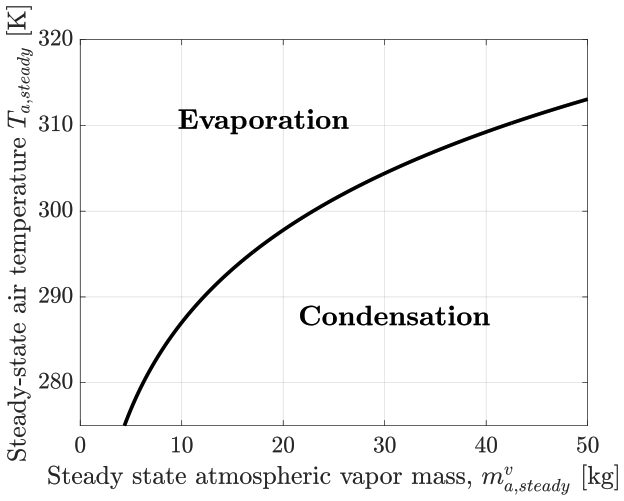
Figure 2 Steady-state air temperature T_a,steady versus atmospheric water vapor mass, $m_{\mathrm{a},\text{steady}}^{\mathrm{v}}$, computed from Eq. (55). The corresponding specific humidity $m_{\mathrm{a},\text{steady}}^{\mathrm{v}}/(m_{\mathrm{a},\text{steady}}^{\mathrm{v}}+m_{\mathrm{a}}^{\mathrm{d}})$ for the range shown varies from 0 (dry) to 2 % (humid).

The dynamical system described by each of the three models, I, A1, and A2, is fundamentally three-dimensional, as the atmospheric vapor mass changes at a rate equal and opposite to that of the oceanic liquid. In the phase space defined by $m_{\mathrm{a}}^{\mathrm{v}}$ (or equivalently $m_{\mathrm{o}}^{\mathrm{l}}$), T_a, and T_o, the steady-state (or neutral) curve shown in Fig. 2 represents the set of equilibrium points where vapor-liquid exchange is balanced. Notably, this curve is independent of the ocean temperature T_o. Consequently, the full three-dimensional steady-state manifold is a surface formed by extruding the neutral curve of Fig. 2 along the T_o axis. However, as discussed below, not all points on this surface correspond to stable equilibria. Moreover, the stability characteristics and dynamical trajectories differ significantly across the three models within realistic regimes of T_a, T_o, and $m_{\mathrm{a}}^{\mathrm{v}}$.

All three eigenvalues of both the current and ideal models are negative along the curve, indicating asymptotic stability (not shown). However, the Jacobian matrix is non-normal, implying that the transient growth due to linear mechanisms can be significant, even though perturbations ultimately decay. As we demonstrate below, these transient amplifications can drive trajectories far from the neutral curve, well beyond the regime of linear validity. In such cases, the full nonlinearity of the governing ODEs governs the long-term dynamics. Due to this non-normality, we do not present a detailed eigenvalue analysis. Instead, we explore the system's behavior geometrically by examining representative trajectories and comparing the the three models through their phase portraits.

Figure 3 shows the evolution of six trajectories for each of the Systems I, A1, and A2, projected onto the T_a–$m_{\mathrm{a}}^{\mathrm{v}}$ plane (left panel) and in the three-dimensional space T_o–T_a–$m_{\mathrm{a}}^{\mathrm{v}}$ (right panel). In the condensation regime (i.e., $T_{\mathrm{a}}<T_{\mathrm{a},\text{steady}}$, below the neutral curve in the left panel), the blue trajectories illustrate that, starting from the initial conditions (black circles), the atmospheric vapor mass decreases in all three models up to their equilibrium values (black diamonds). Conversely, in the evaporation regime (orange trajectories), the vapor mass increases.

As evident from the left panel, condensation is accompanied by an increase in air temperature in all models. The equilibrium T_a in System I lies between those of A1 and A2, with System A1 exhibiting the smallest increase in T_a. Also, in condensation regime, the ocean temperature (blue curves in the right panel) remains largely unaffected across all models. However, model differences become more pronounced in the evaporation regime. When the ocean is colder than the air, evaporation and the associated air–sea enthalpy exchange may produce a weak cooling tendency in the near-surface atmosphere, proportional to the air–sea temperature contrast. This effect is captured by System I through an evaporation-driven T_a tendency term proportional to T_o−T_a. System A2 omits this tendency altogether, which is thermodynamically inconsistent, but not fatal for the present idealized demonstration because the initial temperatures in Fig. 3 are similar (initial T_o=295 K and $\mathrm{280}\lesssim T_{\mathrm{a}}\lesssim \mathrm{300}$), so the resulting change in T_a in the evaporation regime is small. System A1 is more fundamentally flawed in this regime because its evaporation tendency is proportional to $c_{\mathrm{l}}{T}_{\mathrm{o}}-c_{\mathrm{p}}^{\mathrm{d}}{T}_{\mathrm{a}}$. Therefore, as one of the artifacts of using incorrect specific heat capacities (and since $c_{\mathrm{l}}\approx \mathrm{4}{c}_{\mathrm{p}}^{\mathrm{d}}$), A1 predicts an unrealistically rapid increase in atmospheric temperature even when ocean surface is (much) colder.

The reduction in ocean temperature during evaporation is smallest for System I (right panel of Fig. 3). Figure 4 further illustrates the A1 behavior without limiting the display to realistic ranges. From initial conditions above the neutral curve (black circles in the left panel), $m_{\mathrm{a}}^{\mathrm{v}}$ increases as expected, but T_a rises to unphysical values – up to 650 K – before approaching equilibrium at extremely large vapor masses (exceeding the dry air mass $m_{\mathrm{a}}^{\mathrm{d}}=\mathrm{1000}\text{kg}$). Meanwhile, T_o drops to unrealistically low, even negative, values. This behavior results from the evaporation-driven T_a tendency term in Eq. (46). Since $c_{\mathrm{l}}\approx \mathrm{4}{c}_{\mathrm{p}}^{\mathrm{d}}$, typical atmospheric values of T_o and T_a cause this term to push the system away from equilibrium. The trajectory reverses only under extreme conditions where $T_{\mathrm{o}}\lesssim T_{\mathrm{a}}/\mathrm{4}$. The distinction in the evaporation regime across the three systems can be also observed in Fig. 5, where the phase flow at a fixed T_o=295 K points towards the neutral curve in Systems I and A2, but away from it in A1.

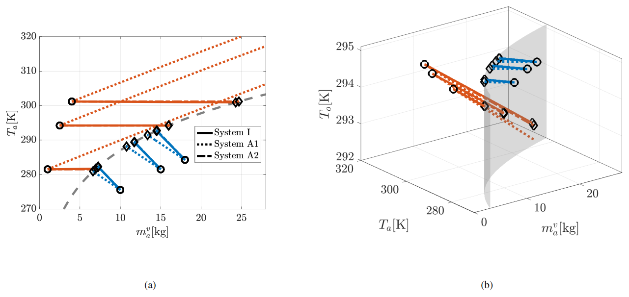
Figure 3 Trajectories in the evaporation (orange) and condensation (blue) regimes predicted by the three models – System I (solid), A1 (dotted), and A2 (dash-dotted) – for realistic values of T_a, T_o and $m_{\mathrm{a}}^{\mathrm{v}}$. (a) Projection onto the T_a–$m_{\mathrm{a}}^{\mathrm{v}}$ plane. (b) Full three-dimensional trajectories in $T_{\mathrm{a}}-T_{\mathrm{o}}-m_{\mathrm{a}}^{\mathrm{v}}$ space. The grey dashed curve (left) and the transparent surface (right) denote the steady-state (neutral) surface. Initial conditions are shown as black circles, and equilibrium points (when reached) as black diamonds.

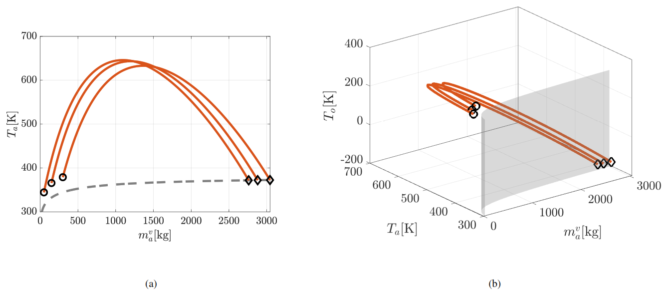
Figure 4 Trajectories of System A1 in the evaporation regime up to the system equilibrium. Same symbols are used as in Fig. 3. (a) 2D projection of trajectories in $T_{\mathrm{a}}-m_{\mathrm{a}}^{\mathrm{v}}$ space, (b) full 3D trajectories in $T_{\mathrm{a}}-T_{\mathrm{o}}-m_{\mathrm{a}}^{\mathrm{v}}$ space.

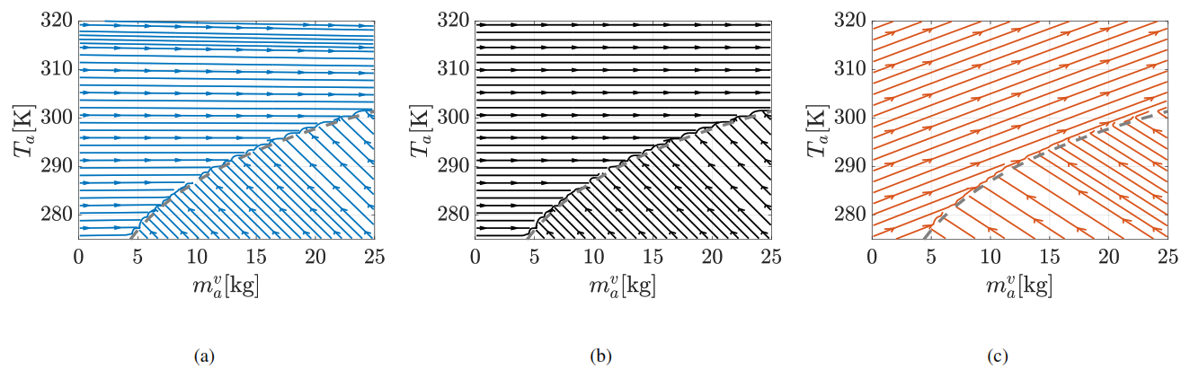
Figure 5 Phase plots in $T_{\mathrm{a}}-m_{\mathrm{a}}^{\mathrm{v}}$ plane of System (a) I, (b) A2, and (c) A1 at T= 295 K. Uneven streamline spacing is an artifact of MATLAB's streamslice function.

Treating System I as the baseline, Fig. 6 quantifies the equilibrium errors in $m_{\mathrm{a}}^{\mathrm{v}}$, T_o, and T_a for System A2 – an E3SM-like system that does not conserve energy. The contours show the percentage change in the equilibrium values of $m_{\mathrm{a}}^{\mathrm{v}}$, T_a, and T_o in System A2 relative to System I, for a fixed T_o=295 K, as a function of the initial atmospheric vapor mass and temperature ($m_{\mathrm{a}}^{\mathrm{v}}$, T_a) shown along the x and y axes, respectively.

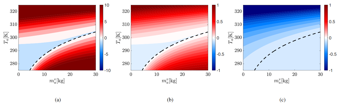
Figure 6 Percentage error in difference between equilibrium values of (a) $m_{\mathrm{a}}^{\mathrm{v}}$, (b) T_a and (c) T_o between Systems A2 and I for initial T_o=295. The x and y axis correspond to the initial T_a and $m_{\mathrm{a}}^{\mathrm{v}}$.

Errors in vapor mass and air temperature are minimal near the neutral curve but grow in both condensation and evaporation regimes. The vapor mass error (left panel) is roughly ten times that of T_a (middle panel), though both share similar spatial patterns. Ocean temperature is underpredicted by 3K (which is around −1 %) for high initial T_a.

Although System A1 conserves energy, its equilibrium errors mirror those in A2 but with significantly larger magnitudes. Figure 7 shows the logarithm of the absolute percentage errors in the equilibrium $m_{\mathrm{a}}^{\mathrm{v}}$, T_a, and T_o, computed for the same set of initial conditions used to visualize System A2's error in Fig. 6. In the condensation regime, errors are small (negative log contours). In contrast, the evaporation regime exhibits extreme errors: where the log of percentage error magnitude reaches 1 for T_a, 5 for T_o and 10 for $m_{\mathrm{a}}^{\mathrm{v}}$. These substantial discrepancies reflect the destabilizing effect of A1's IEFLX evaporation term.

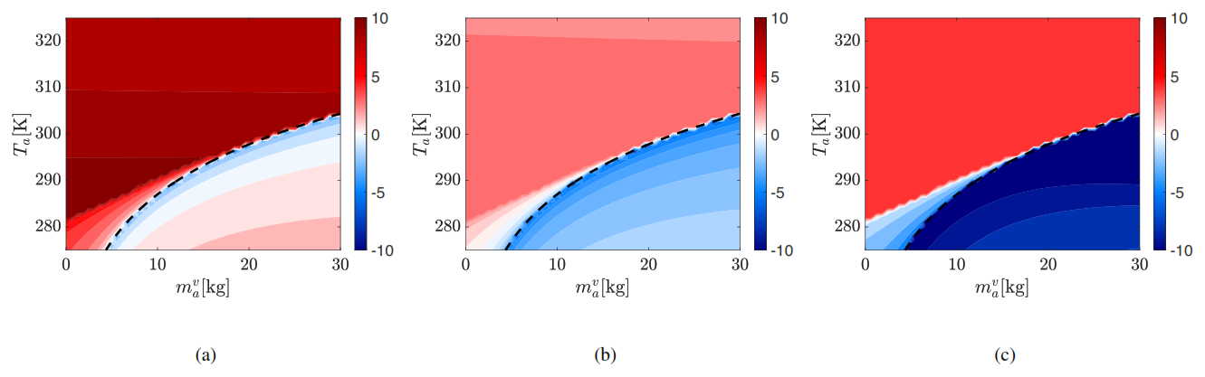
Figure 7 Logarithm of the absolute percentage error in equilibrium values of (a) $m_{\mathrm{a}}^{\mathrm{v}}$, (b) T_a and (c) T_o between Systems A1 and I for T_o=295 K. Axes show initial T_a and $m_{\mathrm{a}}^{\mathrm{v}}$.

Finally, despite showing stability and smaller discrepancy relative to System I, A2 exhibits a net energy loss. Figure 8 (left) shows the percentage change in energy relative to its initial value (with T_o=295 K). A loss of 1 % is observed in evaporation, with smaller losses in condensation. An alternate metric is the temperature leak, defined as

$$\begin{array}{}\text{(56)}& T_{\text{leak}}={\displaystyle \frac{E_{\text{final}}-E_{\text{initial}}}{c_{\mathrm{p}}^{\mathrm{d}}(m_{\mathrm{a}}^{\mathrm{d}}+m_{\mathrm{a},\text{final}}^{\mathrm{v}})}},\end{array}$$

where, E_final−E_initial is the energy lost and $m_{\mathrm{a},\text{final}}^{\mathrm{v}}$ is the final mass of the water vapor in the atmosphere. Shown in the right panel, it ranges approximately from 0–20 K in evaporation and is positive in condensation – qualitatively similar to the energy loss pattern.

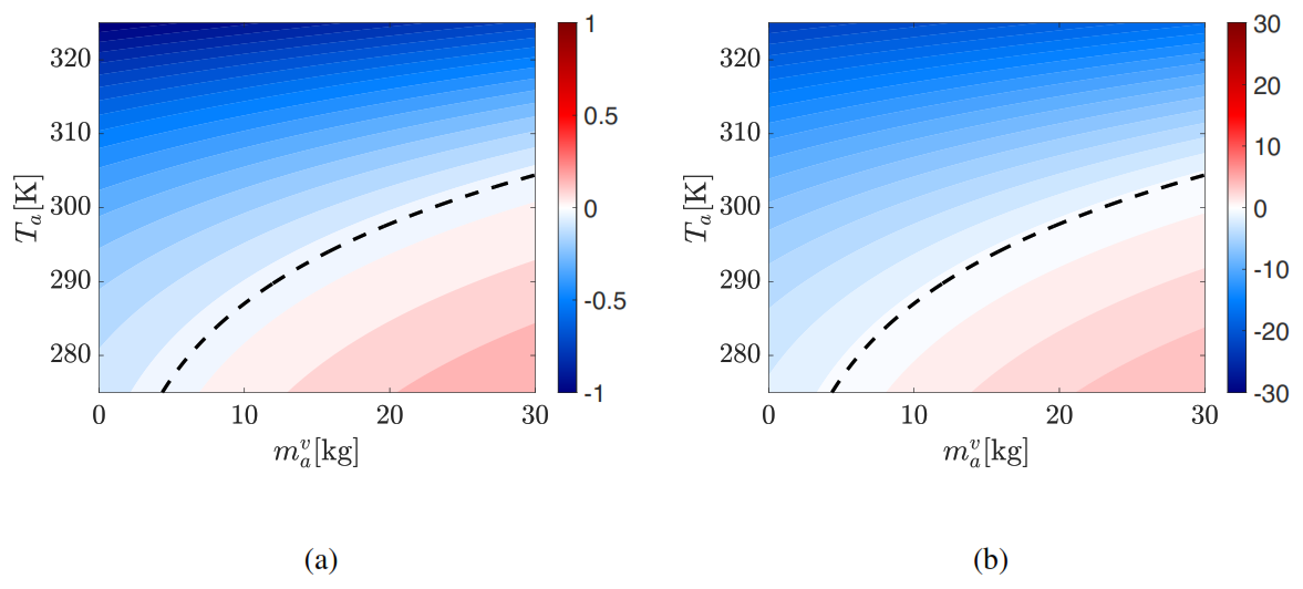
Figure 8 (a) Temperature [K] and (b) percentage energy leak in A2 relative to the energy conserved by A1.

5 Conclusions

In this work, we use a minimal two-box representation of the ocean–atmosphere interface, one atmospheric box and one ocean box, to isolate the energetics of moisture exchange. Our goal is to clarify how thermodynamic approximations used in E3SM enter the coupled energy and mass budgets, and to identify structural consequences of those approximations in a setting where all terms can be tracked explicitly. Starting from a first-principles accounting of energy transfer across the interface in Sect. 2, we derive coupled ordinary differential equations for the evolution of box mass and temperature. Enforcing energy conservation with consistent thermodynamics (Sect. 3.1) leads to an “unapproximated” reference formulation, System I, which closes the energy budget by construction and therefore requires no energy fixers. We then derive an E3SM-analogous formulation (Sect. 3.2), System A1, to make explicit how the model’s thermodynamic simplifications and associated fixers enter the governing equations. Finally, we consider a related formulation without fixers, System A2 (Sect. 3.3), which isolates the consequences of the thermodynamic approximations alone.

Although Systems I, A1, and A2 are highly idealized relative to full E3SM, they provide a transparent framework for interpreting the implications of approximate moist thermodynamics. In our experiments, System A2 behaves similarly to System I in terms of qualitative mass and temperature evolution during both evaporation and condensation, but it exhibits an energy leak during evaporation and an energy gain during condensation, consistent with the missing energetic terms in its formulation. In contrast, System A1 (in our box setting) displays markedly different, physically unrealistic, behavior. This is most apparent during evaporation, where the modeled energetics can imply an increase in atmospheric temperature concurrent with evaporation. The corresponding steady state differs substantially from Systems I and A2, with very low ocean temperatures and a large atmospheric vapor mass. We emphasize that the magnitude and character of this behavior are exaggerated by the box-model structure: in our idealization, any corrective energy is applied within the single atmospheric box, whereas in E3SM the global fixer distributes the aggregate correction across the domain. In the particular case of “A1-like” instability, it is not observed in production E3SM simulations because both energy fixers are applied to the model globally, accounting for both evaporation and condensation at the same time. Since evaporation and condensation rates are close in magnitude and opposite in signs, magnitudes of the fixers are small, and overall the model behaves like System A2.

A natural next step is a controlled E3SM assessment, before and after implementation of the proposed thermodynamic corrections, in the spirit of Harrop et al. (2022). However, such a quantification is challenging in a coupled Earth system model, where multiple components and parameterizations interact, and changes in one component require corresponding updates elsewhere to maintain energy conservation and thermodynamic consistency across modules. Concretely, achieving thermodynamic consistency within E3SM requires the following developments spanning air-sea coupling, vertical transport, phase-change energetics, and package-level closures:

• Implementing transfers of water vapor energy. Implementing the correct evaporation flux, given by Eq. (12), will require moving the energy of the evaporated mass, $c_{\mathrm{p}}^{\mathrm{v}}T\mathrm{\Delta }m+(L_{\mathrm{v}}+L_{\mathrm{l}})\mathrm{\Delta }m$ (Eq. 4), to the atmosphere. However, as discussed in Sect. 2.2.2, there are currently no suitable mechanisms within the atmosphere to absorb the $c_{\mathrm{p}}^{\mathrm{v}}$ term in Eq. (4) in any of parameterizations, including micro- and macrophysics, deep convection, etc. Therefore, we must correctly introduce such mechanisms in the EAM component of E3SM that transport and mix water vapor energy between layers, properly account for it during phase changes, and in turbulence-like parameterizations. This will require an extended effort from atmosphere modelers. Note that even energy-conserving, thermodynamically consistent atmospheric closure schemes for turbulent transport are an underdeveloped field.

• Implementing transfers of energy of other water forms. Similar to that described above for the water vapor, new implementations will need to be made for the energy of falling hydrometeors, cloud water, and cloud ice. While this is an active area of research, several fundamental processes, such as the transfer of kinetic energy and the friction of falling hydrometeros even within the atmosphere, require finalization.

• Validation and verification of new moist-physics packages. The microphysics, macrophysics, convection, etc. packages will need to be modified to account for proposed consistent and unapproximated thermodynamics. These would likely need to be developed first as standalone codes with implementation on idealized and isolated test cases featuring only the relevant physics targeted by the respective package, perhaps in a similar manner to their original development (Morrison and Milbrandt, 2015b; Morrison et al., 2015), before being coupled to operational models like E3SM.

• Tuning E3SM with the new packages. Tuning models as complex as E3SM towards observations remains a significant and necessary step due to uncertainties in Earth system modeling. The new consistent thermodynamics would reduce many of those uncertainties, but would likely not eliminate all of them. We expect that tuning will remain a big part of the Earth system model development even with consistent moist thermodynamics.

A fair comparison of our proposed improvements therefore requires significant development steps – implementation of the concept of moist energy across all components, validation and verification of new components, and retuning of each component and the model as a whole to recover comparable baseline observations. Missing development steps above would result in the model with thermodynamics as crude as the existing one, therefore, invalidating proper comparisons. All of the development stages outlined above are beyond the scope of the present paper.

The broader purpose of this work is to motivate replacement of known deficiencies in approximate moist thermodynamics (as represented here by Systems A1 and A2) with energetically consistent formulations (System I), and to move toward an idealized goal in which the coupled model does not rely on fixers to compensate for evaporation/condensation-related energy imbalances. We hope that our analysis clarifies the relevant energetic constraints and provides a concrete basis for pursuing these developments, enabling simulations that “work for the right reasons” (Harrop et al., 2022).