High-performance coupled surface-subsurface flow simulation with SERGHEI-SWE-RE

This work presents SERGHEI-SWE-RE, a performance-portable, parallel model that couples a fully dynamic two-dimensional Shallow Water Equation (SWE) solver with a three-dimensional Richards Equation (RE) solver within the Kokkos framework to simulate surface–subsurface flow exchange. The model features a modular architecture with sequential coupling strategy, supporting both synchronous and asynchronous executions of surface and subsurface modules. The SERGHEI-SWE-RE model is validated against five benchmark problems incorporating stationary and fluctuating free-surface tests, a tilted v-catchment, a lateral-flow slope without ponding, and a heterogeneous superslab. The results demonstrate good agreement with established models. Asynchronous coupling reduces wall-clock time by up to about 75 % in the superslab case while preserving simulation accuracy. Strong and weak scaling tests on multiple Intel Xeon CPUs and NVIDIA GPUs reveal robust portability, with near-ideal RE scaling and less-satisfactory SWE scaling at high GPU counts, suggesting future improvements on differentiated meshes or more advanced domain decomposition strategies. Overall, the results presented establish SERGHEI-SWE-RE as an efficient, flexible and scalable model for integrated surface-subsurface flow simulations.

1 Introduction

Surface-subsurface water exchange (SSE) is a critical process in the hydrological cycle, which exerts a substantial influence on the dynamics of the water budget and water quality (Dennedy-Frank, 2019; Ntona et al., 2022). In particular, SSE determines in which compartment water volumes are, which in turn has a dominant effect on the time scales of the dynamics of such water volumes. Integrated hydrological models (IH models), since originally conceived by Freeze and Harlan (1969), have been widely used to simulate SSE across diverse scenarios (Paniconi and Putti, 2015; Fatichi et al., 2016), including river basins (e.g., Aliyari et al., 2019; Nixdorf et al., 2017; Gilbert and Maxwell, 2017), lake watersheds (e.g., Autio et al., 2023; Ala-aho et al., 2015; Persaud et al., 2020) and coastal regions (e.g., Daneshmand et al., 2019; Guimond and Michael, 2021; Li et al., 2023; Paldor et al., 2022; Xiao et al., 2017; Yang et al., 2013; Zhang et al., 2018). Valuable insights are also gained from studies on the surface-subsurface coupling algorithms (e.g., Chen et al., 2022; Liggett et al., 2013; de Rooij, 2017). Moreover, IH models are increasingly being integrated with geochemical, ecological and land surface models, facilitating scientific research across a broad range of topics in earth and environmental sciences (e.g., Forrester and Maxwell, 2020; Hein et al., 2019; Naz et al., 2023; Saadi et al., 2023; Zhang et al., 2024).

In IH models, the Shallow Water Equation (SWE) – or its variants – and the Richards equation (RE) (Richards, 1931) are typically employed as the governing equations for surface and subsurface flow, respectively (Haque et al., 2021; Shu et al., 2024). Several reviews have been carried out on this topic, accounting for the different governing equations, and the different approaches to model coupled surface-subsurface flow (Morita and Yen, 2002; Furman, 2008; Shu et al., 2024) and have proposed taxonomies to classify approaches and existing models. Within these taxonomies, of particular interest are the external coupling approach in which the two governing equations are solved independently and exchange information via boundary conditions and source/sink terms, versus the fully coupled or globally implicit approach in which both equations and their boundary conditions and source/sink terms are solved simultaneously. Fully coupled models, such as Parflow (Kollet and Maxwell, 2006), HGS (Brunner and Simmons, 2012; Tang et al., 2024), WASH123D (Yeh et al., 1998; Hussain, 2022), ATS (Coon et al., 2020; Jan et al., 2020), solve the surface and subsurface flow equations simultaneously in a single system (Morita and Yen, 2002; Huang and Yeh, 2009; Shu et al., 2024) and are necessarily synchronous in their time stepping. However, this coupling strategy could be computationally inefficient due to the mismatch between surface and subsurface time scales. That is, surface flow processes are typically faster and more dynamic than subsurface flow. For example, the speed of supercritical shallow water flow could exceed 1 m s⁻¹, but the hydraulic conductivity of the subsurface soil is usually less than 0.001 m s⁻¹ (Furnari et al., 2024). This suggests that the subsurface flow solver could potentially use a larger numerical time step (Δt) than the surface flow solver, without compromising model stability. The fully coupled IH model requires a unified Δt for both surface and subsurface flow, thereby limiting the overall computational speed. In contrast, external coupling strategies can be iterative (e.g., Schüller et al., 2025) and non-iterative (Brandhorst et al., 2021) or sequential approaches. In externally coupled approaches, the SSE is explicitly computed during synchronization to ensure coherence and continuity in the overall simulation. Notable examples include CATHY (Camporese et al., 2010), OpenGeoSys (Delfs et al., 2012), inHM (VanderKwaak and Loague, 2001), and tRIBS+OFM (Kim et al., 2012). This approach offers greater flexibility when modeling either surface or subsurface flow independently (Huang and Yeh, 2009; Shu et al., 2024). Moreover, external coupling also allows for synchronous or asynchronous coupling. That is, it allows different Δt for surface and subsurface calculations, potentially improving computational efficiency. For example, Li et al. (2023) demonstrated that asynchronous coupling can improve computational efficiency by up to 81 % compared to fully coupled approaches.

IH models are typically computationally demanding because of the scale of the study area, especially when the fully dynamic two-dimensional (2D) SWE and the three-dimensional (3D) RE are used. As an alternative, simplified SWEs, such as the diffusive wave or the kinematic wave equation, are widely used to describe surface flow (Maxwell et al., 2014). While these simplifications enable larger Δt, they have limited applicability for rapidly varying flows, such as floods or tidal oscillations (Li and Hodges, 2021). Similarly, some models assume that the subsurface flow is 1D in the unsaturated zone to improve computational efficiency (Ma et al., 2016; Gunduz and Aral, 2005; Kong et al., 2010), but this approximation is inadequate to address pronounced lateral flow in the vadose zone (Mao et al., 2021). Therefore, solving the fully dynamic 2D SWE and 3D RE is indispensable for comprehensive IH models capable of accurately simulating surface hydrodynamics, variable-saturated subsurface flow and surface-subsurface flow exchange under various application scenarios and across scales. Notably, IH models relying on fully dynamic SWE are almost non-existing, with only one known to the authors, limited to 2D SWE coupling to a 1D Richards solver (Crompton et al., 2020). To our knowledge, there is no available model for fully-dynamic 2D SWE solver coupled to a 3D Richards solver.

Recent advances in High-Performance Computing (HPC) technology provide a viable pathway for integrating fully dynamic 2D SWE solvers and 3D RE solvers with acceptable computational cost (Bhanja et al., 2023). Several HPC-based models have been developed and validated through idealized numerical tests and watershed-scale applications (Le et al., 2015; Kuffour et al., 2020; Wu et al., 2021). However, the diversity of modern supercomputing architectures poses challenges for cross-platform portability and broader adoption of these models (Hokkanen et al., 2021). To address these issues, heterogeneous programming models have emerged as effective solutions, offering code portability and hardware independence (Fang et al., 2020). Among these, the Kokkos framework enables performance portability across various manycore architectures for models by providing a unified abstraction for data parallelism and memory access patterns (Edwards et al., 2014). Leveraging Kokkos, Caviedes-Voullième et al. (2023) developed the SERGHEI modeling framework. SERGHEI is an an open-source, high-performance, and performance-portable platform under active development for simulating integrated hydrodynamic, ecohydrologic, and geomorphologic processes. Key components of SERGHEI include a fully dynamic 2D Shallow Water Equation (SWE) solver (SERGHEI-SWE) (Caviedes-Voullième et al., 2023) and a 3D Richards Equation (RE) solver (SERGHEI-RE) (Li et al., 2025). However, the capability of simulating SSE using SERGHEI has yet to be explored and demonstrated.

In this study, we introduce the integrated surface-subsurface flow simulation capabilities of SERGHEI and demonstrate its simulation accuracy, as well as parallel scalability. The integrated model, referred to as SERGHEI-SWE-RE, offers several key advantages:

1. Full dimension, dynamic flow processes: SERGHEI-SWE-RE combines the fully dynamic 2D SWE and 3D RE to simulate coupled surface and subsurface flow. The adoption of these complete governing equations ensures the applicability of SERGHEI-SWE-RE under a wide range of scenarios with various flow conditions.

2. Modularization and flexibility: SERGHEI-SWE-RE uses a sequential surface-subsurface coupling approach and allows asynchronous coupling (see Sect. 2.2 for further details). It offers the flexibility to simulate the integrated system, as well as the surface or the subsurface flow alone. Incorporating asynchronous coupling further enhances the computational efficiency of the integrated simulation.

3. Computational efficiency and portability: SERGHEI-SWE-RE supports performance-portable parallel computation on a variety of computational platforms through the Kokkos framework.

The paper is structured as follows: Sect. 2 describes the governing equations used in SERGHEI-SWE-RE and explains emphatically the details of the coupling strategy. Sections 3 and 4 present the numerical cases and a real-world scenario to support the performance of the integration model. Section 5 presents the conclusions of this paper.

2 Numerical methods

2.1 Surface and subsurface flow

The numerical methods used in SWE and RE modules of SERGHEI have been described in detail in Caviedes-Voullième et al. (2023) and Li et al. (2025), respectively. Herein, we provide a concise overview of the governing equations, numerical schemes, and key solution features.

In SERGHEI-SWE, surface flow is modeled by solving the fully dynamic 2D SWE using a finite volume method for spatial discretization combined with an explicit Euler method for temporal integration. In vector form, the 2D SWE reads

$$\begin{array}{}\text{(1)}& \left\{\begin{array}{l}\frac{\partial \mathbf{U}}{\partial t}+\frac{\partial \mathbf{F}}{\partial x}+\frac{\partial \mathbf{G}}{\partial y}={\mathbf{S}}_{\mathrm{r}}+{\mathbf{S}}_{\mathrm{b}}+{\mathbf{S}}_{\mathrm{f}},\\ \mathbf{U}=\left[\begin{array}{l}h\\ q_x\\ q_y\end{array}\right],\mathbf{F}=\left[\begin{array}{l}{q}_x\\ \frac{q_x^{\mathrm{2}}}{h}+\frac{\mathrm{1}}{\mathrm{2}}g{h}^{\mathrm{2}}\\ \frac{q_x{q}_y}{h}\end{array}\right],\mathbf{G}=\left[\begin{array}{c}{q}_y\\ \frac{q_x{q}_y}{h}\\ \frac{q_y^{\mathrm{2}}}{h}+\frac{\mathrm{1}}{\mathrm{2}}g{h}^{\mathrm{2}}\end{array}\right],\\ {\mathbf{S}}_{\mathrm{r}}\left[\begin{array}{l}{r}_{\mathrm{o}}-r_{\mathrm{f}}\\ \mathrm{0}\\ \mathrm{0}\end{array}\right],{\mathbf{S}}_{\mathrm{b}}=\left[\begin{array}{c}\mathrm{0}\\ -gh\frac{\partial z}{\partial x}\\ -gh\frac{\partial z}{\partial y}\end{array}\right],{\mathbf{S}}_{\mathrm{f}}=\left[\begin{array}{c}\mathrm{0}\\ -gh{\mathit{\sigma }}_x\\ -gh{\mathit{\sigma }}_y\end{array}\right].\end{array}\right.\end{array}$$

where t denotes time [T]; x, y represent the Cartesian coordinates [L]; h signifies the pressure head [L]; The components q_x=hu and q_y=hv represent the unit discharges in x and y directions [L² T⁻¹], respectively; g is the gravitational acceleration [L T⁻²]; r_o represents the rainfall intensity [L T⁻¹] and r_f is the infiltration (or exfiltration) rate [L T⁻¹]; $\frac{\partial z}{\partial x}$, $\frac{\partial z}{\partial y}$ are the bed slope in x and y directions; σ_x, σ_y are the friction slope in x and y directions. The shallow water equation (Eq. 1) is solved with a first-order finite volume scheme (Morales-Hernández et al., 2021). The stability of the scheme is constrained by the Courant–Friedrichs–Lewy (CFL) condition, where a CFL number less than 0.5 is required.

In SERGHEI-RE, subsurface flow is described using the generalized 3D RE as

$$\begin{array}{}\text{(2)}& {\displaystyle \frac{\partial \mathit{\theta }}{\partial t}}+{\displaystyle \frac{S_{\mathrm{s}}\mathit{\theta }}{\mathit{\varphi }}}{\displaystyle \frac{\partial h}{\partial t}}-\mathrm{\nabla }\cdot \left(\mathit{K}\right(h\left)\mathrm{\nabla }\right(h-z\left)\right)-q_{\mathrm{s}}=\mathrm{0}\end{array}$$

where θ is the volumetric water content; S_s is the specific storage capacity [L⁻¹]; ϕ is porosity; h is pressure head [L]; K indicates the hydraulic conductivity tensor [L T⁻¹], which is a function of the pressure head; z represents the elevation head [L]; q_s incorporates source/sink terms [T⁻¹]. It should be noted that this formulation includes the specific storage effects to unify the modeling of both saturated and unsaturated subsurface flow regimes (Krabbenhøft, 2007).

Equation (2) requires a model closure, which is achieved by means of soil-water retention models. In SERGHEI-RE, the popular Mualem–van Genuchten model (Mualem, 1976; van Genuchten, 1980) is adopted to describe the relationship between the pressure head (h), the water content (θ), and the hydraulic conductivity (K) as

$$\begin{array}{}\text{(3)}& \left\{\begin{array}{l}\mathit{\theta }\left(h\right)={\mathit{\theta }}_{\mathrm{r}}+\frac{\left({\mathit{\theta }}_{\mathrm{s}}-{\mathit{\theta }}_{\mathrm{r}}\right)}{{\left(\mathrm{1}+|\mathit{\alpha }h{|}^n\right)}^m},\\ K\left(h\right)=K_{\mathrm{s}}{\left(\mathrm{1}+|\mathit{\alpha }h{|}^n\right)}^{-\frac{m}{\mathrm{2}}}{\left(\mathrm{1}-{\left(\mathrm{1}-{\left(\mathrm{1}+|\mathit{\alpha }h{|}^n\right)}^{-\mathrm{1}}\right)}^m\right)}^{\mathrm{2}},\\ m=\mathrm{1}-\frac{\mathrm{1}}{n},\end{array}\right.\end{array}$$

where the model parameters include the residual water content (θ_r), the saturated water content (θ_s), the saturated hydraulic conductivity (K_s [L T⁻¹]), and two soil-specific parameters (α [L⁻¹] and n).

In SERGHEI-RE, the RE is spatially discretized by a finite volume scheme. For time integration, two numerical schemes are available: (i) the predictor-corrector (PC) scheme that shows superior convergence behavior, but requires a smaller time step size (Δt), and (ii) the modified Picard (MP) iterative scheme that allows for large time steps, but may fail to converge under certain hydrogeological conditions. For a detailed comparison of the two schemes, refer to Li et al. (2024).

2.2 Surface-subsurface exchange

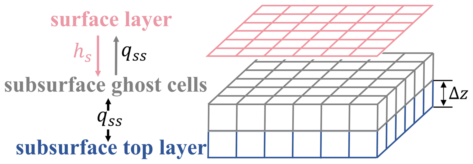
The coupling strategy of SERGHEI-SWE-RE follows an externally coupled, sequential (non-iterative) approach. This means, both solvers are solved independently, and they exchange states and fluxes in sequence, without iterating during a coupling time step. Spatially, the surface and subsurface domains share the same horizontal discretization, both using structured Cartesian grids with uniform grid spacing. After solving the SWE, the surface water depth (h_s) is mapped to the ghost cells of the subsurface grid (gray cells in Fig. 1) to establish the upper boundary condition for the RE solver. Upon completion of the RE solution, the SSE flux (q_ss) is evaluated from the top-layer (h_g) and the ghost cell pressure heads, then passed back to the surface module. Finally, the surface water depth is updated by adding an equivalent depth calculated by integrating q_ss over the coupling time step.

Figure 1 The schematic of data exchange between subdomains.

The complete SSE computation procedure is shown in Fig. 2 and described as follows:

1. Solve the SWE (excluding SSE) to obtain the surface water depth ($h_{\mathrm{s}}^{*}$), and transfer it to the subsurface ghost cell layer. Note that “^*” indicates an intermediate solution of the water depth.

2. Determine the type of boundary condition to be applied to each cell in the top layer of the subsurface domain. To complete this step, SERGHEI first calculates a hypothetical SSE flux ($q_{\mathrm{ss}}^{*}$) based on Darcy's Law (Eq. 4) as

   $$\begin{array}{}\text{(4)}& q_{\mathrm{ss}}^{*}=\mathrm{2}\times K{\displaystyle \frac{h_{\mathrm{g}}-h_{\mathrm{s}}^{*}}{\mathrm{\Delta }z}}-K,\end{array}$$

   where Δz is the height of the top subsurface cell and upward flux is marked positive. Then, there are four possible situations:

   • i.

     If the surface cell is wet, and $-q_{\mathrm{ss}}^{*}\times \mathrm{\Delta }t\le h_{\mathrm{s}}^{*}$, indicating that either exfiltration occurs, or the infiltration volume is less than the available surface water, the ghost layer head ($h_{\mathrm{s}}^{*}$) is used as the pressure head boundary condition for the subsurface domain (Fig. 2b).

   • ii.

     If the surface cell is wet, but $-q_{\mathrm{ss}}^{*}\times \mathrm{\Delta }t>h_{\mathrm{s}}^{*}$, indicating that all surface water infiltrate into the subsurface within the current time step. In this case, using a pressure head boundary condition would overestimate infiltration. Instead, a flux boundary condition is applied to the top subsurface layer, where the SSE flux is set to the equivalent flux of the available ponding depth (Fig. 2c).

   • iii.

     If the surface cell is dry, and $h_{\mathrm{g}}-\mathrm{\Delta }z/\mathrm{2}>h_{\mathrm{s}}^{*}$, indicating that exfiltration occurs, similar to condition (i), the ghost layer head ($h_{\mathrm{s}}^{*}$) is used as the pressure head boundary condition (Fig. 2d).

   • iv.

     If the surface cell is dry, but $h_{\mathrm{g}}-\mathrm{\Delta }z/\mathrm{2}\le h_{\mathrm{s}}^{*}$, indicating that neither infiltration nor exfiltration should occur, a no flow boundary condition is enforced to the subsurface domain (Fig. 2e).

3. Once the type of subsurface boundary condition is determined, solve the RE to update the pressure head.

4. Calculate the final SSE flux, q_ss. For Case (i) and (iii), q_ss is determined using Darcy's Law, similar to Eq. (4). For Case (ii), $q_{\mathrm{ss}}=-h_{\mathrm{s}}^{*}/\mathrm{\Delta }t$. For Case (iv), q_ss=0.

5. Calculate an equivalent SSE depth from the SSE flux, and add it to the surface water depth to get the final surface water depth. That is, $h_{\mathrm{s}}=h_{\mathrm{s}}^{*}+\mathrm{\Delta }t\times q_{\mathrm{ss}}$.

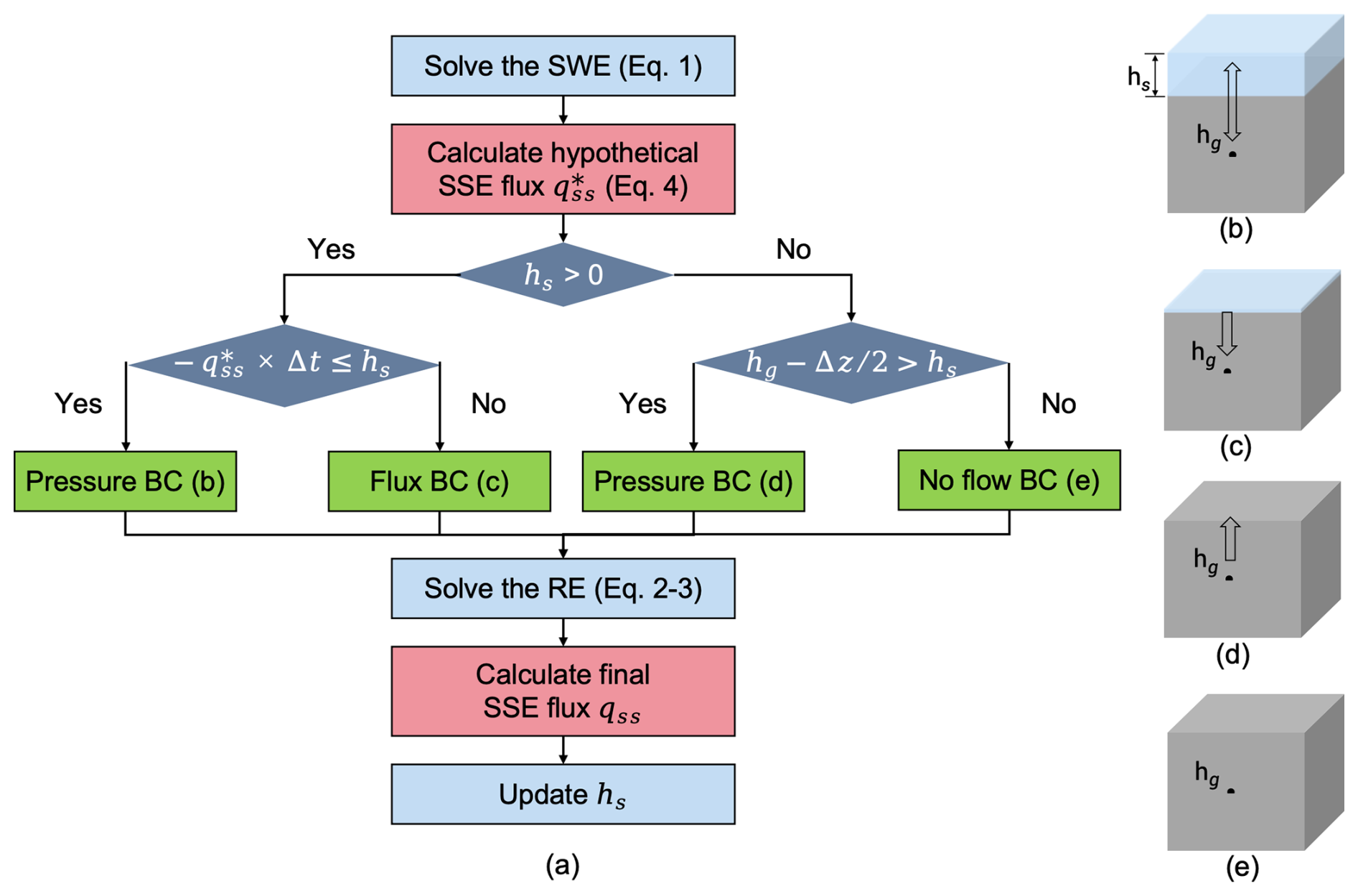
Figure 2 (a) The flow chart of the SSE simulation process. (b–e) Illustrations of the four possible situations where the SSE fluxes are calculated differently.

A special case is the rainfall condition. When the ground surface is dry, rainfall is typically a flux boundary condition to the subsurface domain. In SERGHEI-SWE-RE, for simplicity, it is assumed that rainfall is always applied to the surface domain, accumulates as surface ponding, then infiltration is computed following the above procedure. This avoids the need to handle rainfall in the subsurface solver. It should be noted that numerically, rainfall acts as a source term in the SWE continuity equation. This source term is added after the depth and flux are solved, meaning that it does not affect the SWE momentum equation within the same time step. This ensures that rainfall cannot generate surface runoff before the updated water depth is passed to the RE solver to drive infiltration, indicating that this treatment does not translate into an unphysical lag between rainfall and infiltration.

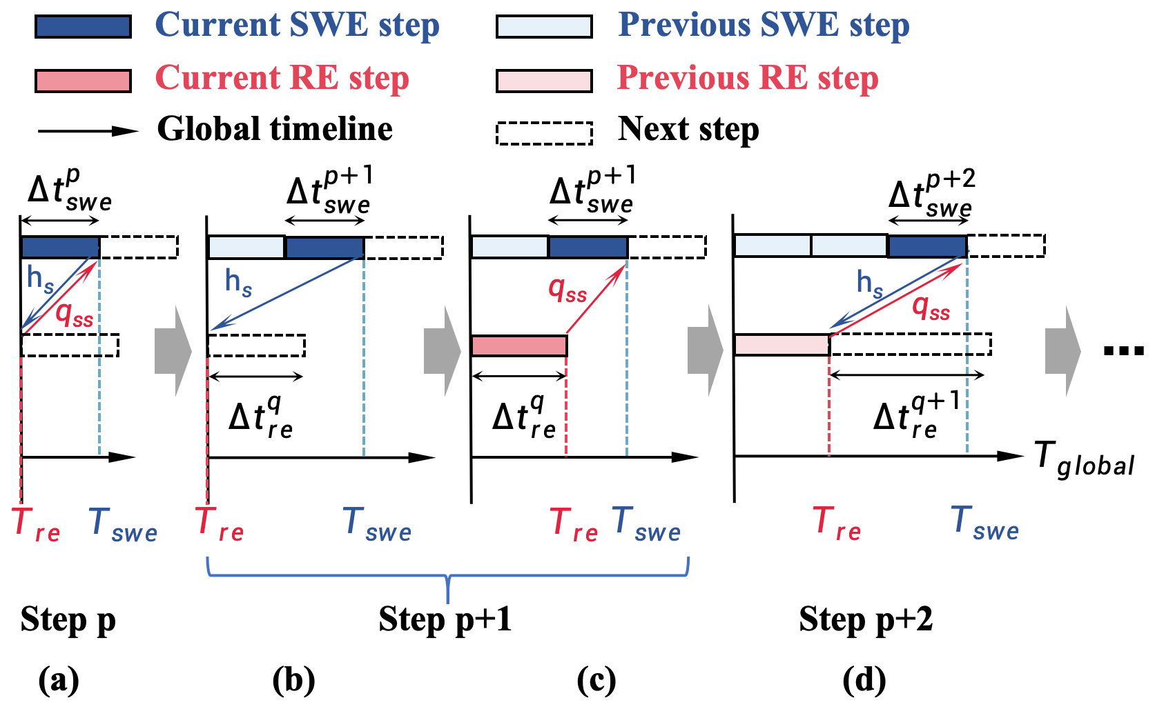
Figure 3 Schematic of the asynchronous coupling strategy between SWE and RE modules over time: (a) when $T_{\mathrm{re}}+\mathrm{\Delta }{t}_{\mathrm{re}}>T_{\mathrm{swe}}$, only the SWE module executes. The surface depth (h_s) is passed to the RE module, while the exchange flux (q_ss) is calculated using the lagged subsurface head from the previous step. This q_ss is passed back to the SWE module for finalizing the surface water depth; (b) as the SWE module advances, the execution condition for the RE module ($T_{\mathrm{re}}+\mathrm{\Delta }{t}_{\mathrm{re}}<T_{\mathrm{swe}}$) is met; (c) the RE module executes using the most recent h_s as a boundary condition. Once the subsurface state is updated, a q_ss is calculated and returned to the SWE module for updating surface water depth; (d) if the next RE step would again exceed the updated surface timeline, the RE module remains stationary while the SWE module continues to advance, re-entering the state described in (a).

SERGHEI-SWE-RE supports both synchronous and asynchronous coupling between surface and subsurface modules. In synchronous coupling, the surface and subsurface modules are executed at every global time step, defined as the smaller of their individual time steps, ensuring both solvers advance on a common timeline. In asynchronous coupling, as shown in Fig. 3, the two modules operate on their own independent timelines, denoted as $T_{\mathrm{swe}}^p=\sum _{i=\mathrm{0}}^p\mathrm{\Delta }{t}_{\mathrm{swe}}^i$ and $T_{\mathrm{re}}^q=\sum _{i=\mathrm{0}}^q\mathrm{\Delta }{t}_{\mathrm{re}}^i$, where p and q are the time step indices and $\mathrm{\Delta }{t}_{\mathrm{swe}}^p$ and $\mathrm{\Delta }{t}_{\mathrm{re}}^q$ are the corresponding time step sizes. Both $\mathrm{\Delta }{t}_{\mathrm{swe}}^p$ and $\mathrm{\Delta }{t}_{\mathrm{re}}^q$ vary in time. The former is restricted by the CFL condition, and the latter is adjusted based on either the maximum change in water content (in the PC scheme) or the number of linearization iterations (in the MP scheme). A user-defined upper bound, Δt_re,max, is enforced to further constrain $\mathrm{\Delta }{t}_{\mathrm{re}}^q$ (Li et al., 2025). The subsurface module is executed only when $T_{\mathrm{re}}+\mathrm{\Delta }{t}_{\mathrm{re}}^q<T_{\mathrm{swe}}$. With this approach, the SSE flux (q_ss) is computed using the current surface flow state and the previous subsurface flow state, shown as the red arrows in Fig. 3. Similarly, the latest surface water depth is sent backward to the subsurface module as boundary conditions, shown as the blue arrows in Fig. 3. Asynchronous coupling significantly enhances computational efficiency by reducing the execution times of the RE module. However, it introduces a time lag of the subsurface module as illustrated in Fig. 3. This time lag inevitably results in coupling errors that depend on both the time scale difference between surface and subsurface flow and the lag duration, an issue extensively discussed in Li et al. (2023) and later in Sect. 3.5. Practically, users can tune Δt_re,max to balance coupling accuracy and computational efficiency. It is, in principle, also possible to set the $\mathrm{\Delta }{t}_{\mathrm{re}}^q=N\mathrm{\Delta }{t}_{\mathrm{swe}}^p$ to prevent an excessive difference between the two time-step sizes. However, investigation of this approach, and a full investigation of the implications of synchronocity/asynchronicity is left for future work. Finally, it is worth noting that the synchronous/asynchronous coupling strategies apply to both PC and MP schemes of the RE solver. For both schemes, the surface water depth is used as a boundary condition for implicitly solving the subsurface pressure head. Consequently, the data exchange pathways between modules, shown as red and blue arrows in Fig. 3, are identical for both solution schemes. The selection of Δt_re,max should be guided by the characteristic time scales of the surface and subsurface dynamics. For environments with highly permeable soils, thin top subsurface layers, or scenarios featuring rapidly varying wetting and drying cycles, a smaller Δt_re,max is required to resolve fast-moving wetting fronts. Conversely, for more stable rainfall-runoff simulations, empirical testing (Sect. 3.5) indicates that Δt_re,max can often be safely set to roughly an order of magnitude larger than the average surface time step without a noticeable loss of accuracy. An associated issue with asynchronous rainfall-runoff simulation is that because the RE solver is not executed at every surface time step under asynchronous coupling, and that rainfall is applied to the surface domain first, rainfall may accumulate and trigger surface runoff prior to the computation of infiltration. However, it will be shown in Sect. 3.5 that when Δt_re,max is set to roughly an order of magnitude larger than the surface time step, this potential discrepancy remains negligible.

It should be noted that sequential coupling, which relies on explicit boundary condition switching, has historically been reported to cause numerical difficulties during rapid state transitions (Furman, 2008). A prominent alternative is to use a fully coupled scheme that eliminates the need for switching. While some fully coupled approaches still face convergence degradation near dry-to-ponding transitions (Coon et al., 2020), recent advances have proposed elegant formulations to bypass these issues completely (e.g., Casulli, 2017; Tubini and Rigon, 2022). Despite these advances, SERGHEI-SWE-RE deliberately uses a sequential coupling scheme to maximize flexibility, as the framework is designed to be highly modular and open-source. Crucially, this externally coupled structure is a prerequisite for supporting asynchronous time-stepping. Furthermore, SERGHEI adopts a non-iterative predictor-corrector scheme for subsurface flow, which inherently avoids the nonlinear convergence failure loops common to popular iterative methods. As demonstrated in Sect. 3, for benchmark tests involving boundary condition switching (Sect. 3.3 and 3.5), SERGHEI-SWE-RE successfully navigates these transitions without generating numerical oscillations, yielding solutions that agree well with established reference data. It must be acknowledged that the modularization of SERGHEI is currently limited to the internal framework. At present, SERGHEI does not natively support standard community interfaces for external coupling, such as the Basic Model Interface (BMI) or OMS3 (Hutton et al., 2020; Tubini and Rigon, 2022; Peckham et al., 2013). Establishing external interoperability through such standardized interfaces remains a long-term development objective for the SERGHEI framework.

2.3 Parallelization

SERGHEI-SWE-RE is built upon SERGHEI-SWE and SERGHEI-RE, achieving portability through the Kokkos framework. For details on the explanation of portability implementation in each module, refer to Caviedes-Voullième et al. (2023) and Li et al. (2025). The model employs uniform structured grids in the horizontal directions for both surface and subsurface domains. Identical horizontal grid resolutions are used across both domains to allow the one-to-one coupling, as described in Sect. 2.2. Variable grid spacing is adopted in the vertical direction of the subsurface domain. When using MPI for distributed memory parallelization, domain decomposition is consistent across both surface and subsurface domains, as illustrated in Fig. 4. The computations within each partitioned subdomain are identical. As emphasized in Li et al. (2025), to ensure the modeling of surface hydrodynamics in all subdomains, domain decomposition is performed only along the x and y directions, with user-defined partition numbers.

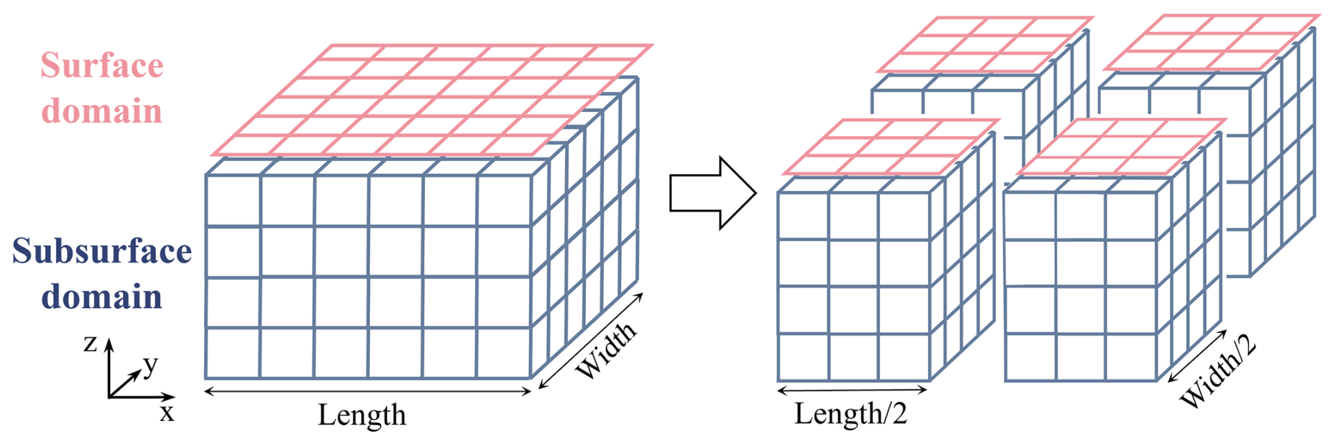
Figure 4 The schematic of SERGHEI-SWE-RE domain decomposition. The surface and subsurface domain decomposition is consistent, with user-defined number of partitions in x and y directions.

3 Model verification

In this section, we evaluate the performance of the SERGHEI-SWE-RE model through five verification cases. Case 1 and Case 2 assess the model's performance under static and dynamic surface water level conditions, respectively, validating its C-property and dynamic performance. Case 3 examines a tilted v-catchment scenario to evaluate the accuracy of infiltration and surface runoff calculations, as benchmarked in Maxwell et al. (2014) and Kollet et al. (2017). Case 4 simulates rainfall on a sloped domain, accounting for both vertical infiltration and lateral subsurface flow motion (Beegum et al., 2018; Brandhorst et al., 2021). Case 5 is the superslab benchmark problem reported in Kollet and Maxwell (2006) and Kollet et al. (2017), featuring heterogeneous soil properties to represent more realistic geological conditions. The following sections provide detailed information on the cases and simulation results.

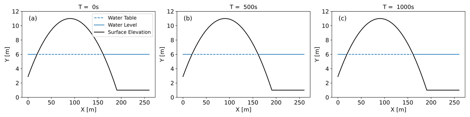
Figure 5 The simulated free surface and groundwater table elevations for Case 1 at (a) T=0 s, (b) T=500 s, (c) T=1000 s on the transect of y=90 m.

3.1 Case 1: stationary simulation

This case study examines a square domain with a bump topography. The domain measures 260 m on each side, with a uniform background bottom elevation (z) of 1 m and impermeable boundaries on all sides. At the point of the domain (90 m, 90 m), a 3D axisymmetric bump rises from the base, following a parabolic profile described by $z(x,y)={\mathrm{bump}}_{\max }\times (\mathrm{1}-r^{\mathrm{2}}/R^{\mathrm{2}})$, where $r=\sqrt{(x-x_{\mathrm{0}}{)}^{\mathrm{2}}+(y-y_{\mathrm{0}}{)}^{\mathrm{2}}}$. The bump has a circular base with radius R=100 m and reaches a maximum height (bump_max) of 10 m above the base level. The soil properties are uniform throughout the domain: α=6 m⁻¹, n=2, K_s=1.5096 m s⁻¹, θ_s=0.3, θ_r=0.08, ϕ=0.3, and $S_{\mathrm{s}}=\mathrm{1.0}\times {\mathrm{10}}^{-\mathrm{5}}$ m⁻¹. Initially, both the surface water level and water table are set at an elevation of 6 m. The simulation runs for 1000 s. Throughout the entire simulation, the maximum absolute deviation of the surface water level from its initial condition remains zero. Figure 5 shows the distributions of surface water level and water table along the transect at y=90 m at T=0, 500, and 1000 s, demonstrating that both the free-surface elevation and subsurface pressure fields are preserved at their initial states. These results confirm that the C-property is satisfied to machine precision.

3.2 Case 2: fluctuating free surface

This test case maintains the same domain configuration as Case 1, except that a fluctuating surface water level is enforced at the inlet boundary located at x=260 m for y ranges from 0 to 260 m, following the hydrograph shown in Fig. 6. As the inlet water level varies, both the interior water level and inundation area change accordingly, causing variations in the water table. Figure 7 illustrates the spatiotemporal variations of surface water depth across the domain. Figure 8 presents the simulation results of the surface water level and the water table at different times along the profile y=90 m. The continuity between the free surface water level and water table is consistently maintained throughout the simulation, demonstrating the reliability of the coupled surface-subsurface flow simulation.

Figure 6 Inlet hydrograph for Case 2.

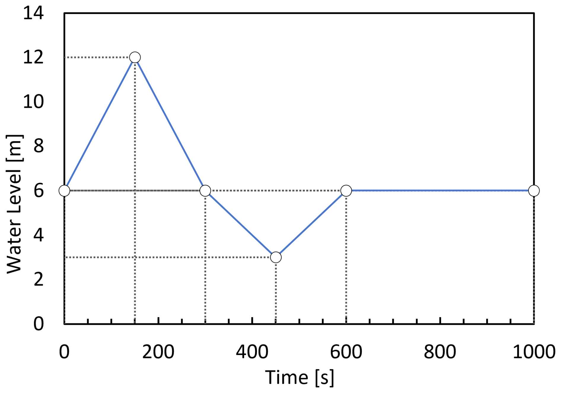
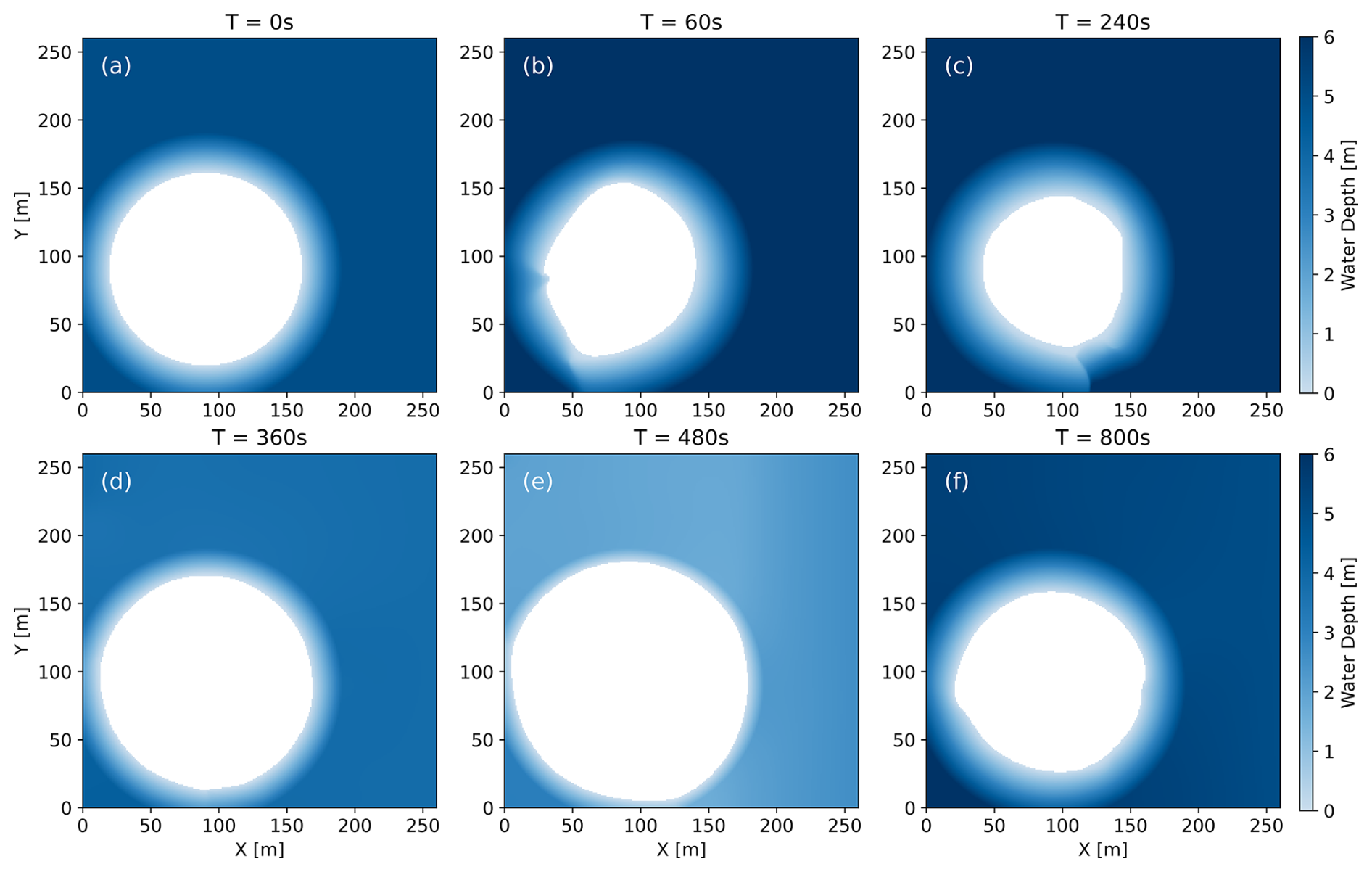
Figure 7 The water depth simulation results for Case 2 at (a) T=0 s, (b) T=60 s, (c) T=240 s, (d) T=360 s, (e) T=480 s, and (f) T=800 s on the transect of y=90 m.

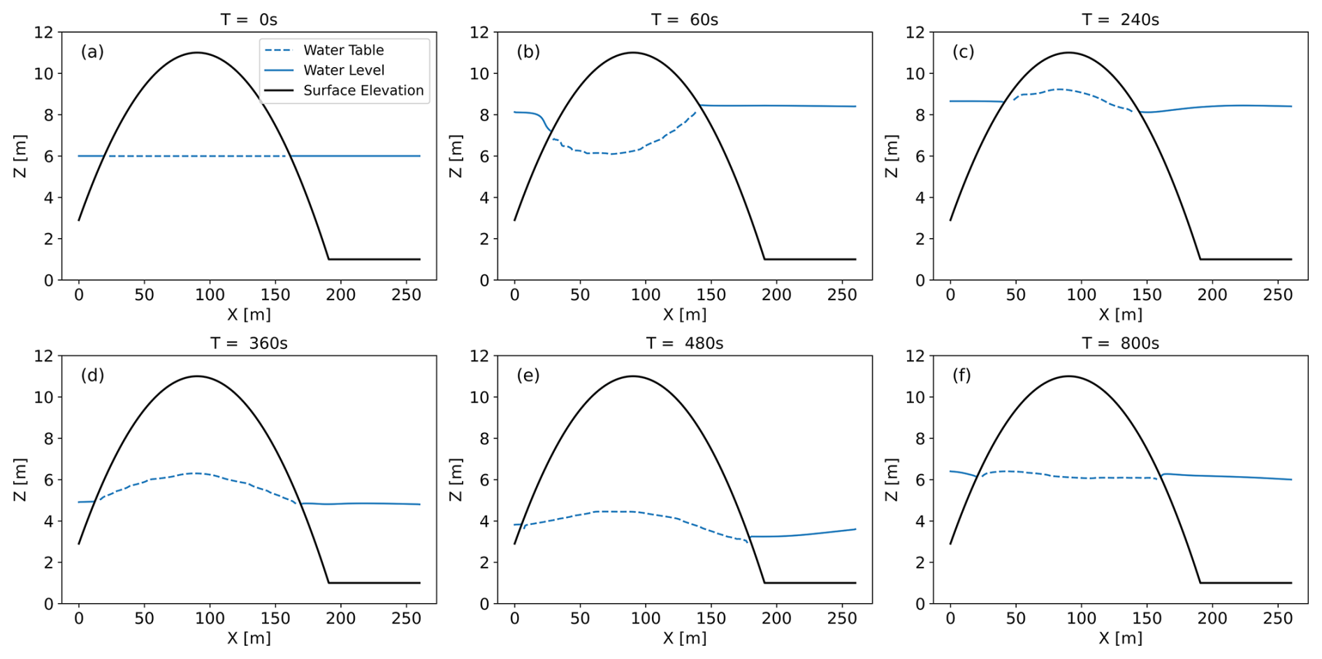
Figure 8 The water table and surface water level simulation results for Case 2 at (a) T=0 s, (b) T=60 s, (c) T=240 s, (d) T=360 s, (e) T=480 s, and (f) T=800 s.

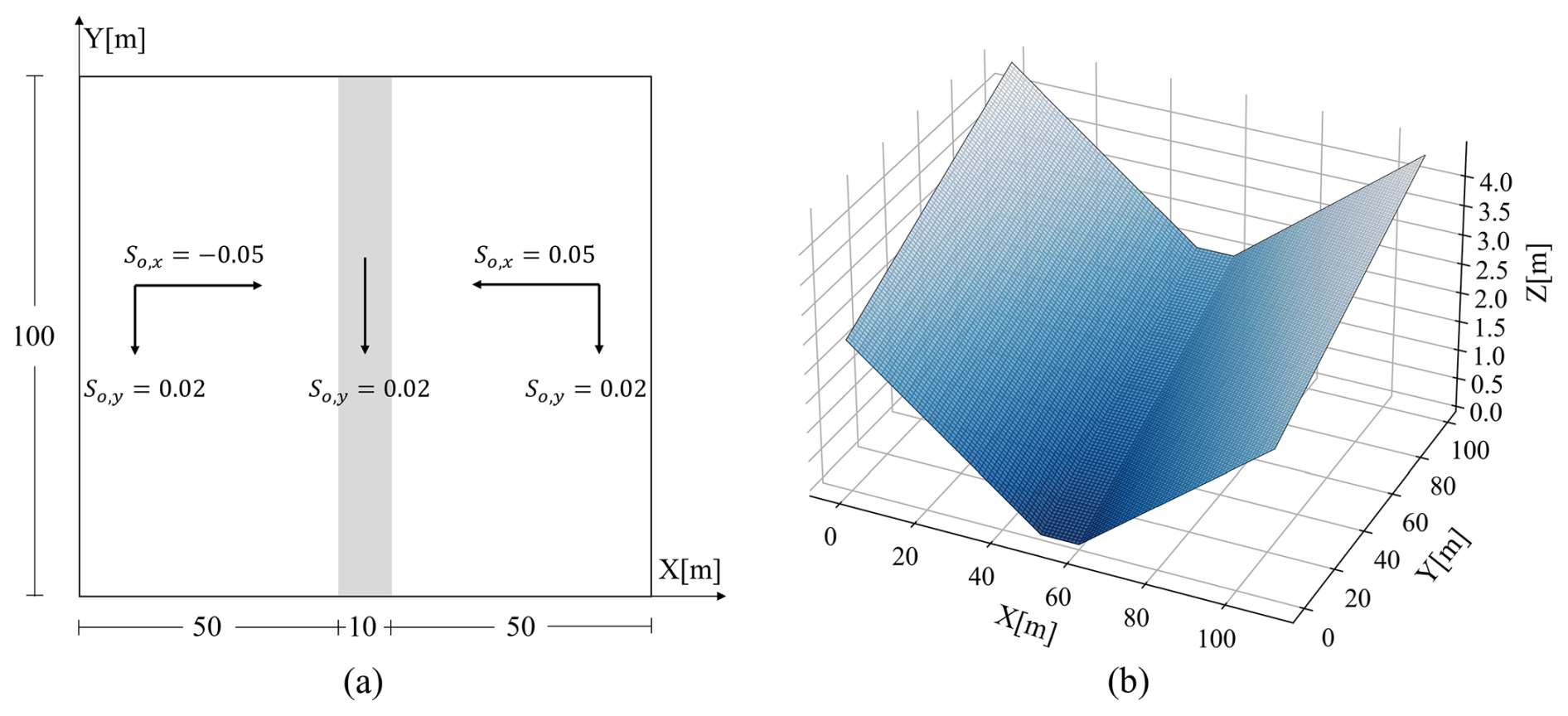
Figure 9 The dimension of the model domain for the tilted v-catchment simulation, modified from Kollet et al. (2017).

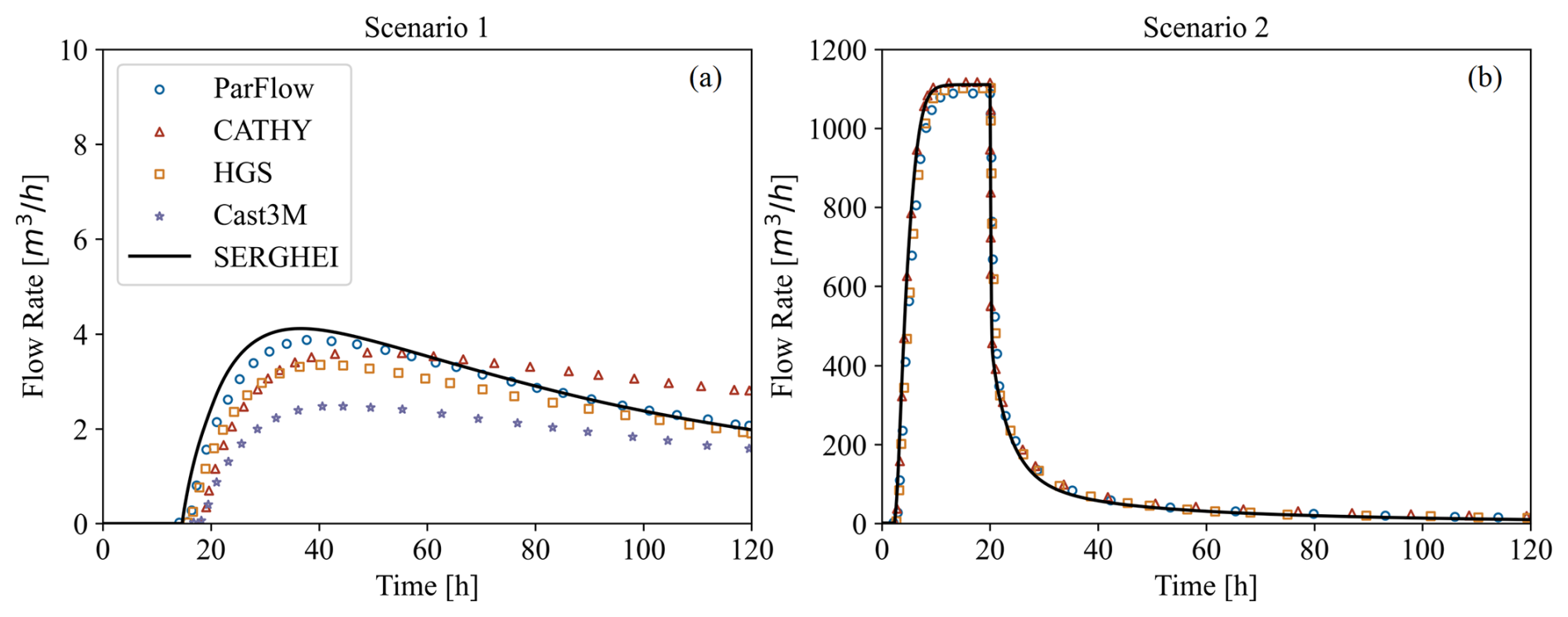
Figure 10 The simulated discharge at the outlets of (a) Scenario 1 (no rainfall) and (b) Scenario 2 (with rainfall).

3.3 Case 3: tilted v-catchment

The tilted v-catchment has been used in the model comparison study of Kollet et al. (2017) for benchmarking coupled surface-subsurface flow simulations. The configuration of the model domain is shown in Fig. 9. The grid resolution is 1 m in both x and y directions. The Manning's coefficient is set to ${\mathit{\mu }}_{\mathrm{1}}=\mathrm{1.74}\times {\mathrm{10}}^{-\mathrm{4}}$ h m${}^{-\mathrm{1}/\mathrm{3}}$ for the slopes and ${\mathit{\mu }}_{\mathrm{2}}=\mathrm{1.74}\times {\mathrm{10}}^{-\mathrm{3}}$ h m${}^{-\mathrm{1}/\mathrm{3}}$ for the bottom channel. The subsurface domain depth is 5 m and is divided uniformly into 25 layers, with a water table 2 m below the surface as the initial condition. The bottom of the subsurface domain is impermeable. The soil is homogeneous, with $K_{\mathrm{s}}=\mathrm{2.78}\times {\mathrm{10}}^{-\mathrm{3}}$ m s⁻¹, α=6 m⁻¹, n=2, θ_s=0.4, θ_r=0.008, ϕ=0.4, and $S_{\mathrm{s}}=\mathrm{1.0}\times {\mathrm{10}}^{-\mathrm{5}}$ m⁻¹.

Two scenarios are established, both with a duration of 120 h. In Scenario 1, the subsurface water moves downstream under gravity and then forms a return flow to the surface domain, resulting in surface runoff at the channel outlet. In Scenario 2, an idealized rainfall with an intensity of 100 mm h⁻¹ is added during the first 20 h, followed by a 100 h recession period. In this case study, the simulation results of SERGHEI-SWE-RE are compared with those of four existing models (ParFlow, CATHY, HGS, and Cast3M) as reported in Kollet et al. (2017).

The simulation results of the discharge at the channel outlet are depicted in Fig. 10. In Scenario 1, the discharge onset time is about T=15 h for SERGHEI-SWE-RE, which aligns well with the other four models. In terms of the discharge hydrograph, SERGHEI-SWE-RE generally matches the results of the other models, with the closest resemblance to ParFlow. In Scenario 2, SERGHEI-SWE-RE has good agreement with all other models in terms of the modeled outlet discharge.

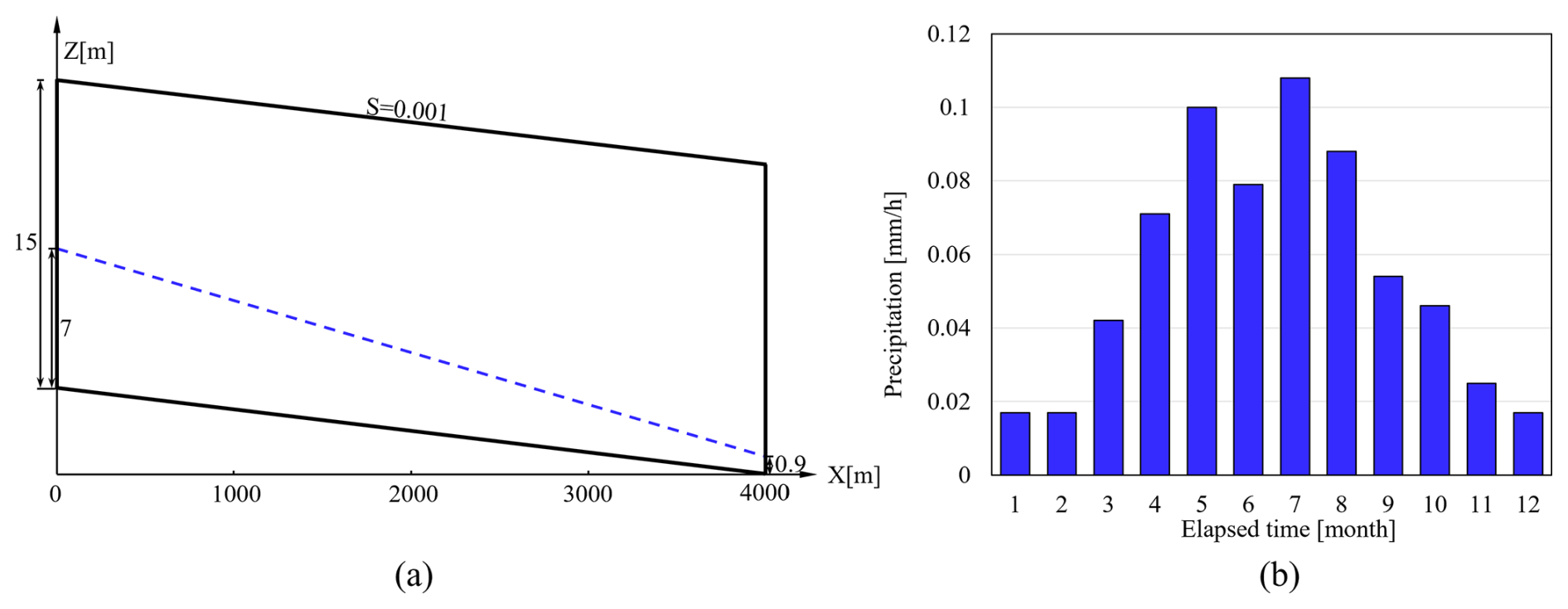
Figure 11 (a) The model domain configuration of the 2D case and (b) the monthly rainfall intensity.

3.4 Case 4: lateral flow

Case 4 models rainfall-infiltration into an inclined slope with open lateral boundaries. The original model domain is 3D, but can be reduced to a 2D x–z simulation due to symmetry. Since the rainfall rate is less than the saturated hydraulic conductivity, no ponding occurs. Thus, this test case can be modeled with a Richards solver only and has been used for verifying SERGHEI-RE (Li et al., 2025). Herein, we reproduce the simulation result by activating the SWE solver, which means that precipitation is first added to the surface domain and then infiltrates into the subsurface through the SSE computation capabilities. As depicted in Fig. 11a, the 2D model domain is 4000 m in length and 15 m in height. The water table elevation is fixed at 7 and 0.9 m on the left and right boundaries, respectively. Hydrostatic pressure distribution is applied below the water table and a constant pressure head of −1.25 m is enforced above the water table. The subsurface domain is divided into 60 layers with uniform grid resolution and homogeneous soil properties: $K_{\mathrm{s}}=\mathrm{5.78}\times {\mathrm{10}}^{-\mathrm{4}}$ m s⁻¹, α=1.65 m⁻¹, n=2, θ_s=0.45, θ_r=0.1, ϕ=0.45 and $S_{\mathrm{s}}=\mathrm{1.0}\times {\mathrm{10}}^{-\mathrm{5}}$ m⁻¹. The simulation spans a 5-year period of continuous rainfall, with a consistent intensity maintained each year. Monthly variations in rainfall intensity are presented in Fig. 11b.

The results of the SERGHEI-SWE-RE calculations are compared with those of the HYDRUS model and SERGHEI-RE as described in Beegum et al. (2018); Li et al. (2025). Given that the entire rainfall infiltrates the subsurface without generating surface ponding or runoff, SERGHEI-SWE-RE and SERGHEI-RE are expected to produce identical results. Figure 12 presents the water table distribution along the x direction at the end of the simulation and its variation at the domain center (x=2000 m). The results demonstrate excellent agreement between SERGHEI-SWE-RE and SERGHEI-RE, while being slightly higher than that of the HYDRUS model. The consistent simulation of lateral seepage flow dynamics validates that SERGHEI-SWE-RE can accurately simulate rainfall that completely infiltrates from the surface and reliably characterize groundwater table dynamics in domains with lateral water flow.

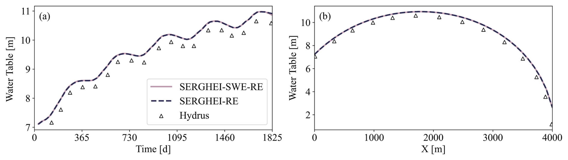
Figure 12 Water table (a) at the domain center and (b) at the end of the simulation along the x direction.

3.5 Case 5: heterogeneous superslab

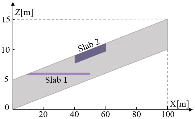
Case 5 considers the superslab benchmark problem reported in Kollet et al. (2017), which consists of rainfall-runoff simulation on a sloped plane. The plane has a length of 100 m in the x direction and a slope of 0.1 (Fig. 13). The Manning's roughness coefficient is $\mathit{\mu }=\mathrm{1.0}\times {\mathrm{10}}^{-\mathrm{6}}$ h m${}^{-\mathrm{1}/\mathrm{3}}$. Two soil slabs (slab 1 and slab 2) are present in the subsurface domain with significantly lower conductivities (K_s) than the background soil. The properties of the soils are detailed in Table 1. The perimeter and bottom of the subsurface domain are impermeable. The simulation period is 12 h, with a constant rainfall intensity of 50 mm h⁻¹ applied for the initial 3 h.

Figure 13 The problem domain configuration of the slab case with three soil types.

Table 1 The specific parameters for soil types.

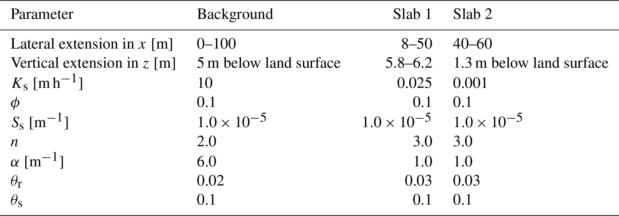
The SERGHEI-SWE-RE simulation result is compared with with five existing models (ATS, CATHY, HGS, Cast3M, and ParFlow) reported in Kollet et al. (2017). For this benchmark problem, ParFlow produces very similar discharge hydrograph and soil saturation profiles to ATS, so it is not displayed herein for simplicity. Furthermore, the simulation results obtained from synchronous and asynchronous coupling approaches are all presented. In synchronous coupling approach, the surface and subsurface solvers are advanced with the same time step. The surface time step (Δt_swe) typically ranges from 0.4 to 0.55 s for this case. In asynchronous coupling simulations, the maximum time step of the RE solver (Δt_re,max) is set to 1, 2, 3 and 4 s, with 4 s roughly an order of magnitude larger than the SWE solver time steps. Due to the high degree of overlap among the results, only the $\mathrm{\Delta }{t}_{\mathrm{re},\max }=\mathrm{4}$ s case is presented for clarity.

Figure 14 shows simulated soil saturation profiles at the outlet (x=0 m), the edge of slab 1 (x=8 m) and the edge of slab 2 (x=40 m), respectively. At all three locations, SERGHEI-SWE-RE remains within the envelope of existing models, and aligns well with the ATS and HGS profiles at x=0 and 8 m. x=40 m is more challenging as the reference models produce divergent saturation profiles (Fig. 14c). Nevertheless, SERGHEI-SWE-RE stays close to most of the reported models, indicating that it is capable of capturing soil water dynamics in heterogeneous soil media.

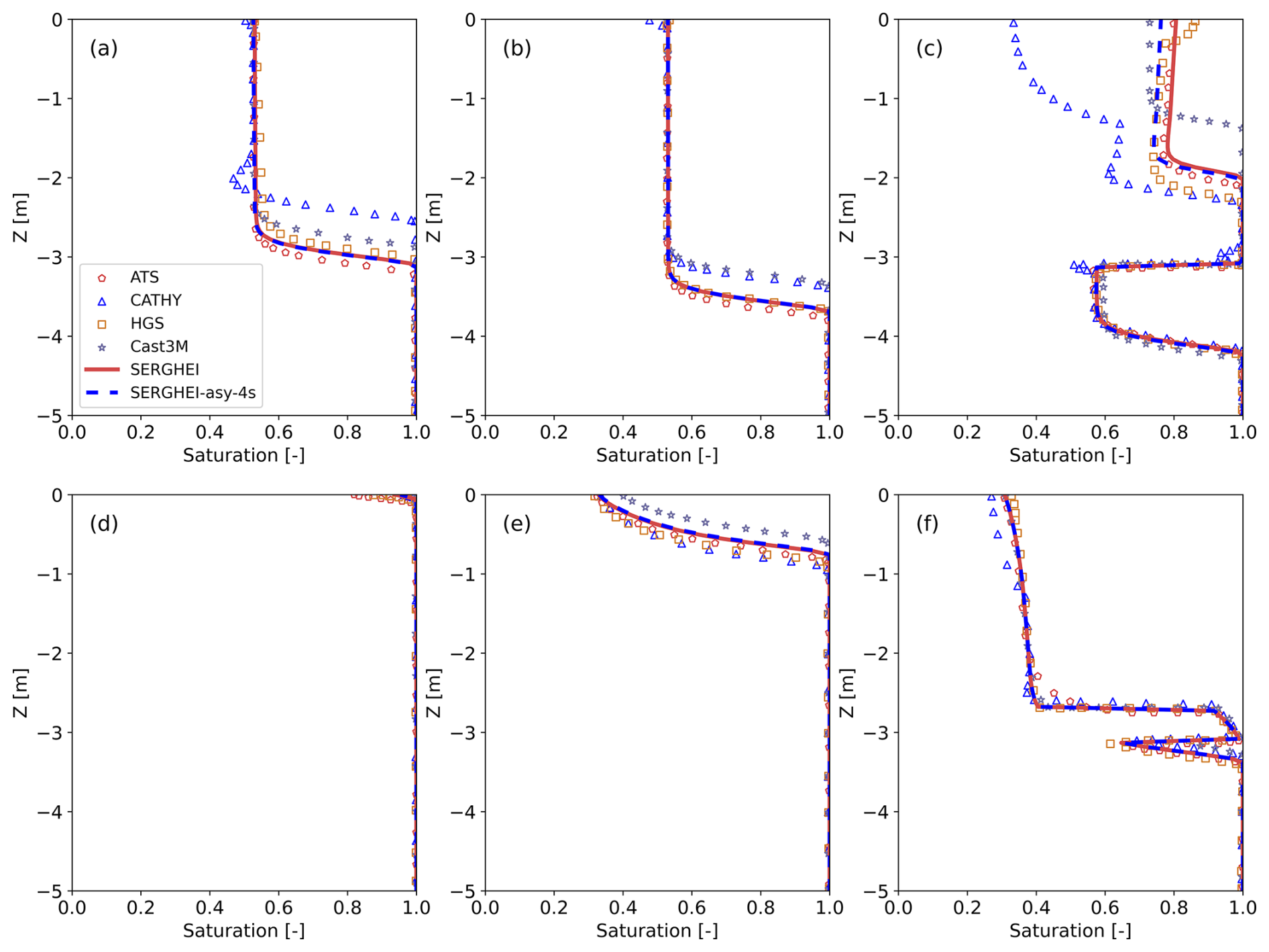
Figure 14 The simulated soil saturation profiles for (a–c) T=3 h and (d–e) T=6 h at X=0, 8, 40 m. SERGHEI represents the synchronous calculation; SERGHEI-asy-4s represents the asynchronous calculation with the $\mathrm{\Delta }{t}_{\mathrm{re},\max }=\mathrm{4}$ s.

Figure 15 presents the simulated outlet discharge and surface water volume. As shown in Fig. 15a, the discharge hydrograph of SERGHEI-SWE-RE aligns well with ATS and Cast3M. In contrast, notable discrepancies are observed when compared to the results from CATHY and HGS. For the surface ponding volume, Fig. 15b shows a significant difference between SERGHEI-SWE-RE and the other models, with SERGHEI-SWE-RE consistently producing higher ponding volumes. In this case, surface ponding primarily arises from the combined effect of direct rainfall and runoff from the upslope. To further investigate the source of the discrepancy, a separate simulation of rainfall-runoff on slab 2 is performed, with infiltration disabled and upslope/downslope sections truncated. The resulting ponding volume, shown as the blue dashed line in Fig. 15b, illustrates that the discrepancy of SERGHEI-SWE-RE persists. Clearly, this discrepancy originates from the SWE solver rather than the SSE coupling. SERGHEI-SWE-RE solves the fully dynamic 2D SWE. In contrast, the benchmark models employ simplified approximations, such as the kinematic wave equations (ParFlow and CATHY) or the diffusive wave equations (ATS, HGS and Cast3M). This indicates that in this case, the simplified equations underestimate the water depth compared to the full SWE, thereby causing less ponding storage. Consistent with this, Caviedes-Voullième et al. (2020) and Li and Hodges (2021) reported that the diffusive wave approximation systematically underestimates water depths compared to the full SWE model in rainfall-runoff simulations. Similarly, de Almeida and Bates (2013) showed that simplified models (including diffusive wave equations and local inertial models) underestimate water depth gradients under unsteady conditions, leading to reduced ponding. Therefore, the model discrepancy in Fig. 15b does not undermine the validation of SERGHEI-SWE-RE for reliable surface–subsurface exchange simulations. In contrast, it underscores the need for the full SWE to resolve surface water dynamics, which is essential for accurate surface–subsurface exchange modeling. It also prompts the need to further conduct cross-model comparisons for coupled surface-subsurface models under more dynamic flow conditions, since kinematic and diffusive wave approaches are far more prevalent.

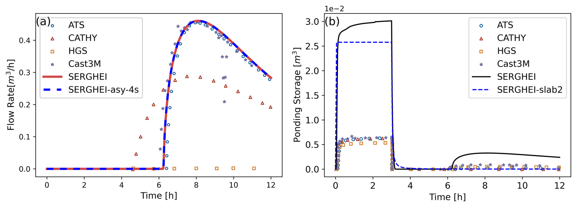
Figure 15 The temporal variations in (a) outlet discharge and (b) surface water volume. SERGHEI represents the synchronous calculation; SERGHEI-asy-4s represents the asynchronous calculation with the $\mathrm{\Delta }{t}_{\mathrm{re},\max }=\mathrm{4}$ s. SERGHEI-slab2 is a customized SWE-only simulation on the slab 2, with the upslope and downslope sections truncated.

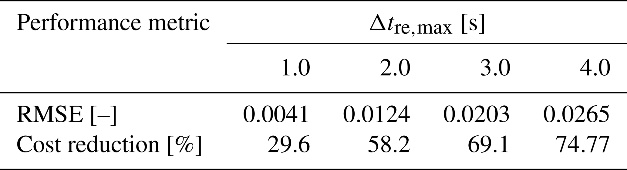
As shown in Figs. 14 and 15, although the synchronous and asynchronous coupling results of SERGHEI-SWE-RE are slightly different, they both achieve satisfactory agreement with existing models in simulating soil saturation and outlet discharge. Table 2 evaluates the performance of asynchronous coupling by comparing the root mean square error (RMSE) of the saturation profiles for T=3 h at X=40 m against the synchronous simulation benchmark. The improvements in computational efficiency are also reported. As expected, while the simulation time reduces as Δt_re,max increases, the RMSE also rises. However, for this test case, the RMSE remains relatively low and the saturation profiles for different Δt_re,max values are nearly indistinguishable (Fig. 14). The reason is that for this rainfall-runoff scenario, the surface flow field is relatively stable. In contrast, under scenarios with highly dynamic surface flow, such as tidal oscillations, asynchronous coupling may lead to non-negligible errors as demonstrated in Li et al. (2023). The optional asynchronous coupling strategy implemented in SERGHEI-SWE-RE thus provide the flexibility that allows users to balance computational efficiency and accuracy for different simulation scenarios. A full investigation of the possible implications of asynchronicity under a set of diverse problems and conditions warrants a study in itself, and sets clear future work to be carried out. In such investigation it will be important not only to document the error and computational efficiency behaviours in response to asynchronicity, but also to explore potential heuristics to optimise this tradeoff.

Table 2 The RMSE in modeled saturation and the reduction in the computational cost for asynchronous coupling with different Δt_re,max.

4 Scalability analysis

4.1 Strong scaling behavior

We evaluate the scalability and performance portability of SERGHEI-SWE-RE through large-scale simulations of Lake Taihu, located in the Yangtze River Delta, encompassing coupled surface-subsurface flow dynamics. In collaboration with the Taihu Basin Monitoring Center of Hydrology and Water Resources, we are developing a coupled surface-subsurface flow model for Lake Taihu using SERGHEI-SWE-RE. Although the complete model is not available yet, the semi-finished model is adequate for conducting scaling tests, which involve fairly complex topography and multiple realistic boundary conditions.

The model domain encompasses an area of approximately 5500 km² and extends to a depth of 30 m. Vertically, the subsurface domain is discretized into 10 layers with variable grid resolutions ranging from 1 to 7.45 m. Horizontally, two grid resolutions are used (Δx=200 and 50 m), resulting in a total of 1 521 828 and 24 349 248 grid cells (including both surface and subsurface domains), respectively. To construct the Lake Taihu model, we integrate topographic data provided by the Taihu Lake Authority for the submerged lake bottom with a freely available 30 m resolution digital elevation model (DEM) data for the surrounding area. We merge the 30 major rivers that connect to the lake into 9 artificial rivers. We also merge the inflow and outflow rate data provided by the Taihu Lake Authority, and distribute the flow rates to the 9 rivers, making sure that the total inflow and outflow of the lake are close to the real conditions. We delineate 15 sections of subsurface boundaries where a prescribed water table elevation is enforced. Due to data limitations, the soil properties across the entire study area are assumed to be uniform. Evaporation and rainfall are neglected for simplicity. A wind subroutine is implemented into SERGHEI-SWE to simulate the wind-driven oscillation of the lake water level, see Eq. (5):

$$\begin{array}{}\text{(5)}& \begin{array}{rl}& {\mathit{\tau }}_x=C_{\mathrm{D}}{\mathit{\rho }}_{\mathrm{a}}\cos \mathit{\omega }{\left(u_{\mathrm{w}}-\left|u\right|\cos \mathit{\beta }\right)}^{\mathrm{2}}\\ & {\mathit{\tau }}_y=C_{\mathrm{D}}{\mathit{\rho }}_{\mathrm{a}}\sin \mathit{\omega }{\left(u_{\mathrm{w}}-\left|u\right|\cos \mathit{\beta }\right)}^{\mathrm{2}}\end{array}\end{array}$$

where, τ_x and τ_y are the wind stresses in x and y directions [M L⁻¹ T⁻²], ρ_a is air density [M L⁻³], u_w is wind speed [L T⁻¹], $\left|u\right|$ is water speed [L T⁻¹], ω is the angle from the x axis to the wind direction, β is the angle between the wind direction and the water flow direction, C_D is the wind drag coefficient, and is set to 0.0013 in this simulation. To avoid instability, wind stress is deactivated if the water depth is less than 0.1 m (Li and Hodges, 2019).

For the scaling tests, Lake Taihu is simulated for 10 d on three HPC facilities: (i) a small cluster at the high-performance computing center of Tongji University (named TJ HPC hereafter), where each CPU node is equipped with an Intel Xeon Max 9468 processor (3.5 GHz, 48 cores, 96 threads), and each GPU node is equipped with an Nvidia L40 GPU (48 GB memory, 864 GB s⁻¹ bandwidth, 18176 CUDA cores), (ii) the LISE HPC system of the German National High Performance Computing (NHR) Alliance at Zuse Institute Berlin, Germany. Each computation node of LISE is equipped with two units of Intel Xeon Platinum 9242 processors (2.30 GHz, 48 cores, 96 threads), and (iii) the JUWELS booster system at the Jülich Supercomputing Center. Each JUWELS booster node contains 4 Nvidia A100 Tensor Core GPU cards (80 GB memory, 1935 GB s⁻¹ bandwidth).

Figure 16 illustrates the simulation time and speedup achieved on the TJ HPC (Δx=200 m). It is evident that, on a single CPU node, the scaling is nearly ideal up to 16 threads. However, starting from 32 threads, the scaling begins to deteriorate. A closer examination reveals that the SWE solver demonstrates poorer scaling compared to the RE solver. The SWE solver exhibits poor scaling due to: (i) lower computational workload due to fewer surface grid cells (than the subsurface domain), (ii) lower computational intensity per grid cell, (iii) higher communication-to-computation ratio, and (iv) load imbalance in boundary condition processing. Indeed, even poorer scaling is observed for the computation of the boundary conditions (BC), because the number of boundary cells is much fewer than the number of interior cells. A similar trend is observed on the GPU, where the speedup of the coupled model exceeds 128, but the speedup of the SWE solver is only around 64, and the speedup of the BC computation is less than 8. It is important to note that the total computational workloads for BC and the SWE solver are significantly smaller than those for the RE solver. Although the BC and the SWE solver are less efficient with an increasing number of threads, the overall scaling of the coupled simulation is predominantly influenced by the scaling of the RE solver.

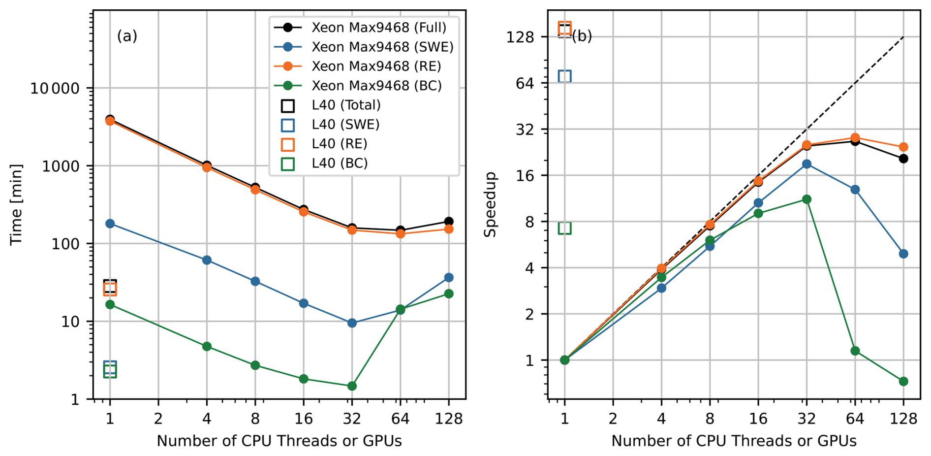
Figure 16 (a) Simulation time and (b) speedup for the Lake Taihu simulation (Δx=200 m) on the TJ HPC. Full, SWE, RE, and BC in the legends represent the simulation time and the speedup of the entire simulation, the SWE solver, the RE solver and the computation of the boundary condition, respectively. Note that the horizontal axis is the number of CPU threads (i.e., the number of CPUs times the number of threads used per CPU) or the number of GPUs. The dashed line represent the ideal scaling.

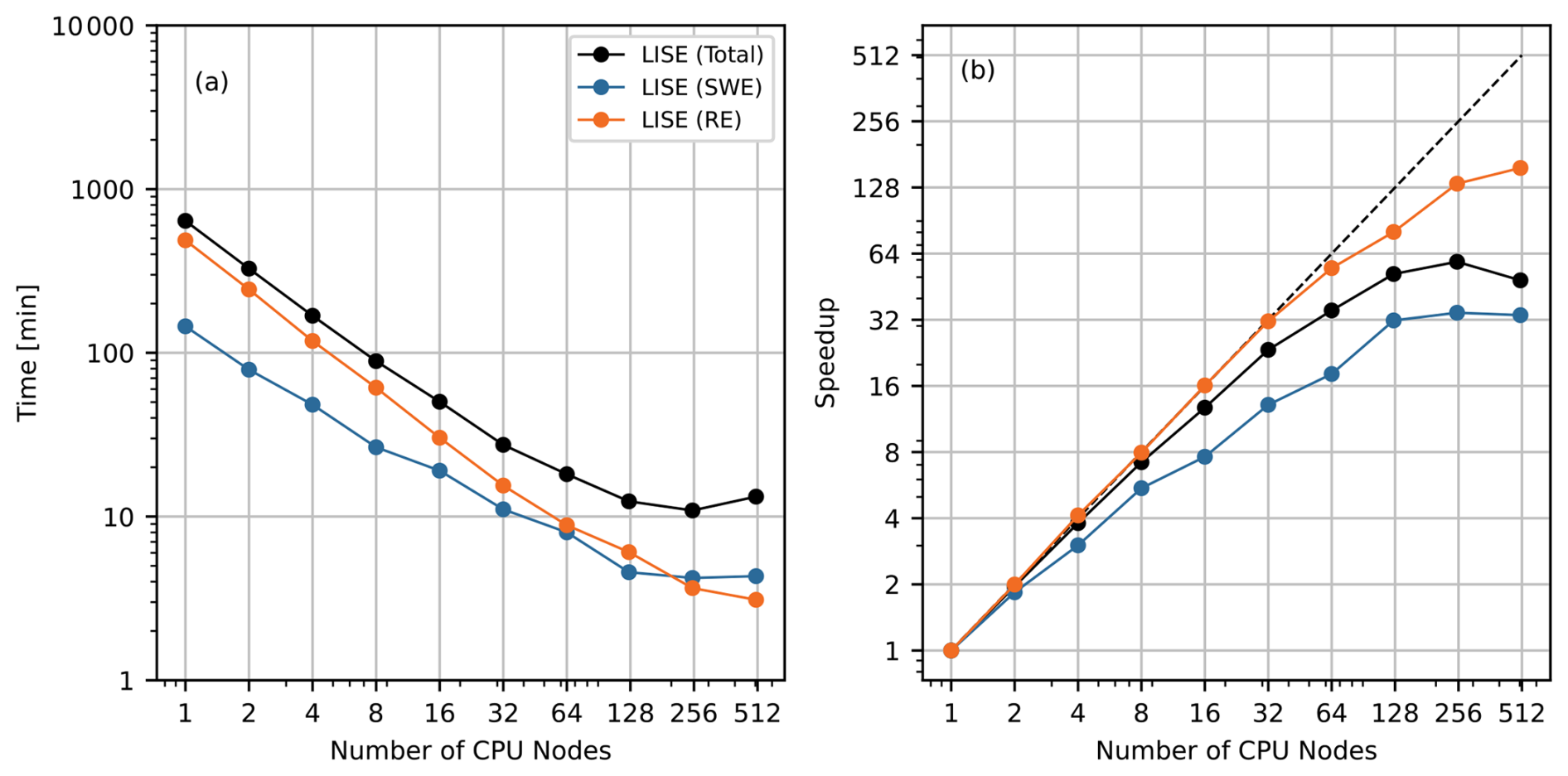
Figure 17 (a) Simulation time and (b) speedup for the Lake Taihu simulation (Δx=50 m) on the LISE HPC with Intel Xeon Platinum 9242 processors. Full, SWE and RE in the legends represent the simulation time and the speedup of the entire simulation, the SWE solver and the RE solver, respectively. The dashed line represent the ideal scaling.

Figure 17 shows the simulation time and speedup on the LISE HPC (with Δx=50 m). The scalability evaluation reveals that both the SWE and RE solvers maintain favorable scalability until deterioration occurs at 64 CPU nodes. In particular, the RE solver exhibits superior scalability compared to the SWE solver, a finding consistent with the observations in Fig. 16. This phenomenon, previously analyzed in relation to Fig. 16, can be attributed to the significantly higher count of grid cells in subsurface computations relative to the surface grid. A comparative analysis between Figs. 16 and 17 indicates that LISE HPC achieves better scalability than TJ HPC, especially for the SWE solver, which is primarily due to the substantial increase in computational grid cells (from 1 521 828 cells at Δx=200 m to 24 349 248 cells at Δx=50 m).

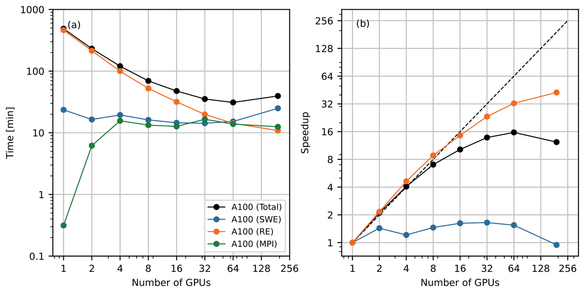
Figure 18 (a) Simulation time and (b) speedup for the Lake Taihu simulation (Δx=50 m) on the JUWELS Booster with Nvidia A100 GPUs. Full, SWE, RE and MPI in the legends represent the simulation time and the speedup of the entire simulation, the SWE solver, the RE solver, and the MPI communication (for both SWE and RE solvers), respectively. The dashed line represent the ideal scaling.

Figure  18 presents the GPU acceleration performance on the JUWELS system. Analysis reveals distinct computational characteristics between solvers: the RE solver demonstrates superlinear speedup (2–8 GPUs) with significantly reduced computation time, while the SWE solver shows minimal improvement and even exhibits increased simulation time at 256 GPUs. Again, this performance divergence stems from the different number of grid cells in the surface and subsurface domains. The surface domain contains only about 2 million grid cells, which is insufficient to fully utilize the computational power of multiple Nvidia A100 GPUs. Figure 18 also illustrates that as the number of GPUs increases, the MPI communication time (including both surface and subsurface domains) approaches the SWE solver computation time, indicating that MPI communication overhead becomes a bottleneck for scaling with more GPUs. For coupled surface-subsurface flow simulations, the number of subsurface cells equals the number of surface cells multiplied by the number of subsurface layers. Consequently, the optimal parallelization configuration for the RE solver becomes inefficient for the SWE solver due to significant disparities in the computational workloads. It indicates that the simple consistent surface-subsurface cell mapping and domain decomposition strategy (Figs. 3 and 4) might be sub-optimal for large-scale parallelization.

This scaling bottleneck highlights a broader architectural limitation in SERGHEI-SWE-RE. The consistent domain decomposition was initially chosen to provide a simple one-to-one mapping between surface and subsurface cells, allowing efficient local data exchange without additional inter-module MPI communication. It limits scalability when their optimal configurations differ and hinders future extensibility, including the potential integration of external coupling interfaces. To address these load imbalances and support broader interoperability, future versions will transition to a flexible exchange architecture that supports (i) different horizontal mesh resolutions and (ii) independent, workload-based domain decompositions.

Although the SWE solver scales poorly on multi-GPU system, the overall speedup is acceptable up to 64 GPU nodes because the computational load of the SWE solver is much less than the RE solver. Moreover, compared to Fig. 16, multi-GPU computing remains faster than multi-thread CPU computing, despite the former consists of 16 times more grid cells (Δx=50 and 200 m respectively). The scaling test results (Figs. 16 to 18) illustrate that SERGHEI-SWE-RE is capable of performing large-scale, coupled surface-subsurface flow simulations on a variety of HPC systems.

4.2 Weak scaling behavior

A second scaling analysis is performed to demonstrate the weak scaling behavior of SERGHEI-SWE-RE. The 2D x–z domain of the lateral flow problem (Sect. 3.4) is extended and duplicated along the y axis to create a 3D test case, where each vertical layer (x–z) is identical. Thus, by adjusting the number of vertical layers in the y direction, the dimension of the computational domain can be customized to maintain the same workload per processor, without affecting the simulation results. A similar domain configuration approach has been reported in Li et al. (2025).

The weak scaling test is conducted on the JUWELS booster system. The domain dimensions are adjusted to ensure that each GPU node is responsible for a subdomain containing 4.8 million subsurface cells and 80 thousand surface cells. Figure 19 shows the parallel efficiency – defined as the ratio between single-node and multi-node execution times – as a function of the number of GPU nodes used. It can be seen that the parallel efficiency of the entire model slightly decreases as more GPUs are employed, but remains higher than 0.8 with 16 GPU nodes, indicating that SERGHEI-SWE-RE can efficiently handle larger problems as the available computational resources increase. The parallel efficiency of the RE solver closely matches the overall efficiency. The SWE module exhibits more variations in the parallel efficiency, but since the simulation time for the SWE solver is relatively small compared to the RE solver, this has a negligible impact on the overall efficiency.

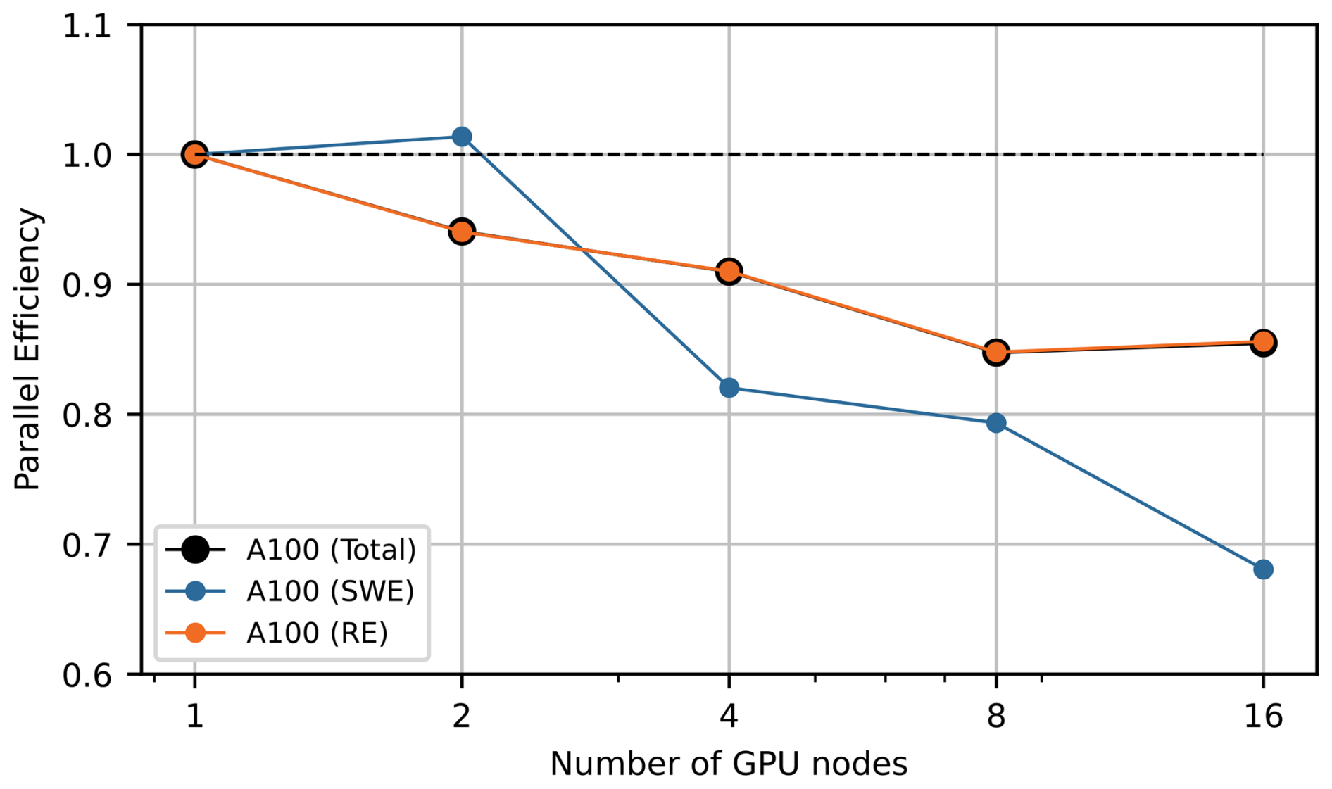
Figure 19 Parallel efficiency for the weak scaling tests performed with the extended lateral flow problem, on the JUWELS Booster with Nvidia A100 GPUs. Full, SWE and RE in the legends represent the efficiency of the entire simulation, the SWE solver and the RE solver, respectively. The dashed line represent the ideal efficiency.

4.3 Coupling overhead and performance impact

The coupling between the SWE and RE modules may introduce additional computational overhead that affects scalability. An additional scaling test is conducted to compare the performance of the coupled model and the standalone SERGHEI-RE module. The problem setup is identical to the lateral flow test (Sect. 3.4), in which rainfall infiltrates into the subsurface without causing surface runoff. Section 3.4 has demonstrated that SERGHEI-RE and SERGHEI-SWE-RE produce indistinguishable water table evolution. However, in SERGHEI-RE, rainfall is applied directly to the subsurface domain as a flux boundary condition, whereas in SERGHEI-SWE-RE, rainfall is first applied to the surface domain, inducing ponding before infiltrating into the subsurface through surface–subsurface exchange computations. To understand the scaling behaviors of these two approaches, the original 3D model domain is used, which spans 4000 m × 5000 m in the horizontal directions and 15 m in the vertical direction. The domain is discretized with uniform grid spacings of $\mathrm{\Delta }x=\mathrm{\Delta }y=\mathrm{5}$ m and Δz=1.5 m, resulting in a total of 8 million grid cells. Figure 20 shows the simulation times and speedups of the two approaches as the number of CPU threads increases. The SERGHEI-SWE-RE and SERGHEI-RE models exhibit negligible difference in terms of both the computational time and the speedup. This behavior can be attributed to the relatively small number of surface grids cells (as discussed in Sect. 4.1) and the absence of surface runoff generation in this case. These results indicate that, for this particular test case, surface–subsurface coupling does not degrade model scalability.

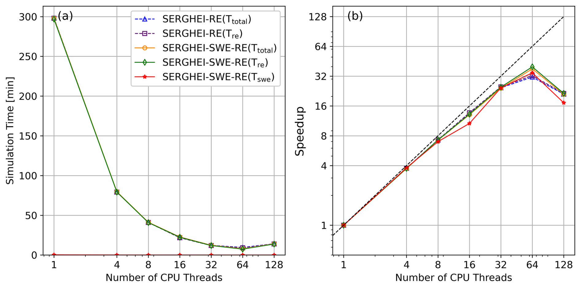
Figure 20 (a) Simulation time and (b) speedup for the Case 4 (3D domain). The black dashed line represents the ideal scaling.

It should be noted, however, that this conclusion applies only to this specific test scenario. In a broader context, surface-subsurface coupling is not expected to alter the scalability of the subsurface module because the SERGHEI-RE solver treats surface flow as a boundary condition (Sect. 2), which must be defined regardless whether SERGHEI-SWE is activated or not. Conversely, the surface module performs an additional parallel loop over all surface grid cells to incorporate the exchange flux as a source/sink term in the mass conservation equation. Thus, if SERGHEI-SWE scales poorly (as shown in Sect. 4.1 on JUWELS), surface-subsurface coupling is expected to further deteriorate the overall scaling performance.

From an HPC perspective, what is considered an overhead may vary. Arguably, inefficiencies due to load imbalance can be viewed as an overhead, e.g., attempting to use a resource set which provides high parallel efficiency for both solvers would likely result in a longer RE runtime. Whether this is an overhead or an inefficiency is a gray area. In any case, this can of course be alleviated by having different sets of resources for each solver (which is not explored in this paper). This in turn links to an undeniable overhead: the exchange of information between the solvers. When both solvers are mapped to the same hardware (i.e., with the same horizontal domain decomposition) as in these tests, this overhead is negligible. However, if states and fluxes must be exchanged through MPI across different resources (CPUs or GPUs), this overhead will grow.

5 Conclusions

In this paper, we introduce an integrated surface-subsurface hydrodynamic model, SERGHEI-SWE-RE, based on the fully dynamic 2D shallow water equation solver (SERGHEI-SWE) and the 3D Richards equation solver (SERGHEI-RE), utilizing the Kokkos framework. The externally coupled model employs a sequential coupling approach, offering both synchronous and asynchronous coupling modes. The coupled surface–subsurface flow exchange simulation results reach good agreement with existing models on the benchmark problems tested, encompassing both homogeneous and heterogeneous soil conditions, as well as scenarios with and without rainfall. The results also suggest potential differences between surface-subsurface models depending on how surface flow is formulated, i.e., typically kinematic and diffusive wave approaches in contrast to the fully dynamic approach adopted herein. This warrants further investigation.

Our tests demonstrate that the asynchronous coupling strategy significantly improves computational efficiency, though it inherently introduces a temporal lag in surface-subsurface exchange. The choice of the coupling time step must balance computational gains with model discrepancies. Future work will comprehensively explore this trade-off and provide more quantitative criteria for optimizing time-stepping for the coupled simulation.

The parallel scalability and performance portability of the model are further evaluated using a real-world case study involving over 24 million grid cells on multiple HPC systems. The results indicate that SERGHEI-SWE-RE performs efficiently across various HPC platforms with different hardware architectures. The SWE solver generally scales poorer than the RE solver due to much less computational workload. Further enhancements on scaling can be expected by improving grid partitioning strategies between the surface and the subsurface domains and mapping the solvers to different computational resources, which is strongly facilitated by the externally coupling strategy.