Validation strategies for deep learning-based groundwater level time series prediction using exogenous meteorological input features

Due to the growing reliance on machine learning (ML) approaches for predicting groundwater levels (GWL), it is important to examine the methods used for performance estimation. A suitable performance estimation method provides the most accurate estimate of the accuracy the model would achieve on completely unseen test data to provide a solid basis for model selection decisions. This paper investigates the suitability of the following performance estimation strategies (validation methods) for predicting GWL: blocked cross-validation (bl-CV), repeated out-of-sample validation (repOOS) and out-of-sample validation (OOS). The strategies are tested on an one-dimensional convolutional neural network (1D-CNN) and a long-short-term memory (LSTM) network. Unlike previous comparative studies, which mainly focused on autoregressive models, this work uses a non-autoregressive approach based on exogenous meteorological input features without incorporating past groundwater levels for groundwater level time series prediction. A dataset of 100 GWL time series was used to evaluate the performance of the different validation methods. The study concludes that bl-CV provides the most representative performance estimates of actual model performance compared to the other two validation methods examined. The most commonly used OOS validation yielded the most uncertain performance estimate in this study. The results underscore the importance of carefully selecting a performance estimation strategy to ensure that model comparisons and adjustments are made on a reliable basis.

1 Introduction

The utilization of machine learning (ML) approaches to predict groundwater levels (GWL) has increased over the last two decades (Tao et al., 2022). The variety of prediction models ranges from simple methods such as tree-based models (e.g. Moghaddam et al., 2022) to more complex deep learning (DL) methods such as artificial neural networks (ANN) (e.g. Derbela and Nouiri, 2020; Iqbal et al., 2020; Nair, 2016), long-short-term memory (LSTM) networks (e.g. Vu et al., 2021; Wunsch et al., 2021; Zhang et al., 2018; Gholizadeh et al., 2023) or one-dimensional convolutional neural networks (1D-CNN) (e.g. Wunsch et al., 2021; Sun et al., 2019; Gomez et al., 2024). According to the review study by Tao et al. (2022), the most commonly used input features for GWL prediction are historical GWL (34 %), precipitation (23 %) and temperature (15 %). Depending on the type of aquifer and the geographical location of the GWL observation well, other features such as sea level or groundwater abstraction rates are also used as input features (Tao et al., 2022). In GWL prediction, we are faced with an increasing number of potential prediction models, a growing number of hyperparameters for increasingly complex models, and a large number of possible input features. In order to find the right method for a particular application, it is necessary to compare the individual methods and to evaluate the results correctly. There is a general consensus on the usual approach to selecting an appropriate prediction method, described for example in Chollet (2021): (i) Select a model, appropriate hyperparameters (e.g. learning rate, batch size, hidden size, number of epochs) and a set of promising input features. (ii) Train the model on the training data set. (iii) Evaluate the performance based on prediction error on the validation data set (validation error). To select an appropriate method, steps (i) to (iii) can be performed several times with different model configurations and compared on the basis of the validation error. Since fitting the model based on the validation error may result in overfitting to the validation data set, the final model should be retested on a completely unknown test data set to obtain the final model error and to get an idea of the generalization ability of the model (Chollet, 2021). Splitting the data into training, validation, and test sets ensures that the model is ultimately evaluated on completely unseen data.

As model fitting and selection should only rely on training and validation data, an appropriate validation method is required to provide an accurate and robust estimate of the error the model would produce on completely unseen data. The choice of the optimal validation method depends primarily on the prediction problem and the characteristics of the data. For time-series, and particularly hydro(geo-)logical time series, which often exhibit autocorrelation and non-stationarity, performance estimation becomes challenging.

Standard out-of-sample validation (OOS), in which part of the latest data is reserved for validation and older data is reserved for training (Tashman, 2000), is often used in groundwater level prediction (Ahmadi et al., 2022). However, this approach can be problematic if exceptional years, such as very dry periods with low groundwater recharge, occur for example only in the validation or test set but not in the training data. This situation leads to a distribution imbalance between training, validation, and test data, which can significantly skew performance estimates. Also the hyperparameters selected based on the validation phase may not have been determined optimally, which, in addition to the distorted performance estimate, also limits the generalization ability of the model on unseen data (Shen et al., 2022). To mitigate this risk, alternative strategies such as cross-validation (CV) or repeated out-of-sample validation (repOOS) can be employed. While standard CV is popular for independent and identically distributed (i.i.d) data (Arlot and Celisse, 2010) and beneficial for small datasets (Chollet, 2021; Bergmeir et al., 2018), its naive application to time series is problematic because it disrupts temporal dependencies and may allow future data to predict the past (Arlot and Celisse, 2010; Chollet, 2021). In addition, the aspect of potential non-stationarity (changing mean and variances over time or presence of long-term trends) is generally not taken into account in CV (Bergmeir and Benítez, 2012). Modified approaches like blocked cross-validation (bl-CV) (Snijders, 1988) preserve temporal structure by avoiding random shuffling, enabling more robust validation for dependent data. Earlier studies from other domains have shown that CV methods are the most reliable performance estimators for autoregressive prediction of stationary time series (e.g. Bergmeir and Benítez, 2012; Bergmeir et al., 2014; Cerqueira et al., 2020). For the autoregressive forecasting of non-stationary time series, on the other hand, according to Cerqueira et al. (2020), the repOOS method provided the most accurate estimates. In these studies, different model types were examined, including linear models, support vector regression, multilayer perceptrons, rule-based methods, and ensemble methods such as random forest models (Bergmeir and Benítez, 2012; Bergmeir et al., 2014, 2018; Cerqueira et al., 2017, 2020). To the best of the authors' knowledge, there is no study in the domain of GWL time series prediction that systematically compares different methods for performance estimation. This research gap is addressed by the present work.

We demonstrate the applicability of k-fold bl-CV for GWL time series prediction and enable a direct comparison with simple OOS validation, the most commonly used method for performance estimation in GWL prediction (Ahmadi et al., 2022), as well as with repOOS, which has been identified as the most accurate method for autoregressive prediction of non-stationary time series in the study by Cerqueira et al. (2020). Previous comparative studies have been limited to autoregressive forecasting approaches (e.g. Bergmeir and Benítez, 2011, 2012; Bergmeir et al., 2014, 2018; Cerqueira et al., 2020). In contrast, this study applies a non-autoregressive approach, which assumes that future groundwater levels are significantly influenced by past meteorological events – particularly precipitation and temperature. Accordingly, only meteorological input features are used. A practical advantage of this approach is the ability to make long-term predictions (e.g., for 10, 50, or 100 years) based on climate scenarios. A 1D-CNN and LSTM model are employed as time series prediction models. These architectures have not been considered in any of the previous comparative studies, but have been proven to be reliable and robust for GWL prediction before (e.g Wunsch et al., 2021). By comparing OOS, bl-CV, and repOOS, this study contributes to methodological development in hydrogeological research by explicitly basing performance estimation on a real-world application in GWL time series prediction. The investigations are based on GWL time series from 100 groundwater monitoring wells in the federal state of Brandenburg (Germany), which were classified as stationary (constant mean and variance over the entire series) or non-stationary (changing mean and variance over the entire series) using a global stationarity assessment.

The following research questions are to be answered in the course of this work:

• Are there differences in the quality of the performance estimates of the three tested validation methods in the GWL time series prediction?

• Which validation method provides the most robust performance estimate in general, for stationary and for non-stationary groundwater conditions?

• Do our results agree with the results of previous studies in the field of autoregressive time series forecasting in other disciplines, or are there differences?

2 Theory and Background

2.1 Validation methods

2.1.1 Out-of-sample validation (OOS)

The standard type of OOS refers to a validation process in which the data set is chronologically divided into subsets. After separating the test data, which often represents the most recent data, the older part of the remaining data is used as training data, while the newer part is used for validation. With the OOS, the validation error of the individual validation data set at the end of the time series is obtained as the performance estimate (see Fig. 1a). The training and validation subsets are often divided according to percentage of the total data set (e.g. 80 % training data and 20 % validation data). A division of subsets by calendar year, to account for seasonal behavior in environmental time series, is also common practice (e.g. Wunsch et al., 2021; Gomez et al., 2024). The OOS approach is most straightforward, as it comes closest to the actual application of time series forecasting, namely predicting the future from the past. In addition, this approach takes into account the assumption that the future is linked to the past and that past processes therefore influence the future. The weakness of OOS is that the validation data set may differ in its properties from those of the training and test datasets, and the resulting validation error could be unrepresentative (Bergmeir and Benítez, 2012).

For a more robust performance estimate, it is recommended to apply the OOS strategy to multiple validation periods (Tashman, 2000). One possible approach for this is the repOOS approach, in which the OOS validation is performed multiple times with different, possibly overlapping training and validation periods (Cerqueira et al., 2017, 2020). This is done by randomly selecting a split point from an available split window within the time series. A fixed fraction (e.g. 60 %) of the data before this split point serves as the training data set and a fixed fraction (e.g. 10 %) after this point serves as the validation data set. Thus, the length of the available split window is limited by the size of the training and validation data (Cerqueira et al., 2017, 2020). The final validation error of the repOOS is the mean of the validation errors of all repetitions. The splitting scheme for one repetition of repOOS validation is illustrated in Fig. 1b.

2.1.2 K-fold blocked cross-validation (bl-CV)

When using standard k-fold CV, the dataset is split into k equally sized, non-overlapping subsets (folds). Typically, the data is shuffled randomly before creating these folds. After splitting, k−1 folds are used for training, while the remaining fold serves as validation data. In time series forecasting, however, random shuffling can be problematic because it breaks the temporal dependencies within the data. If future values of the target variable are to be predicted from past values of the input features, the chronological input–output relationship must be preserved. This holds for both sequence-based time series models and models that work with simpler input–output pairs (e.g., multilayer perceptrons or random forests). Randomly mixing a time-ordered dataset before constructing these pairs is therefore not appropriate. Once input-output pairs have been generated in a temporally consistent way, they can be randomly shuffled, provided that potential overlaps between training and test data are considered. We describe this procedure in more detail in the next section, Sect. 2.2. The correctly aligned input–output pairs can then be used in the usual manner with the respective prediction models.

Alternatively Snijders (1988) used k-fold CV, where the data is not randomly shuffled before being divided into folds. Without random shuffling, the temporal relationship within the folds is preserved, only the temporal relationship between the folds is interrupted. This method is referred to in the literature as blocked cross-validation (bl-CV) (e.g. Bergmeir and Benítez, 2012; Cerqueira et al., 2020). An example of a k-fold bl-CV (k=5) is shown in Fig. 1c. Regardless of whether the data were shuffled before splitting or not, a k-fold CV results in k validation errors, one for each split. To obtain a final performance estimate, the mean of the k validation errors is calculated. The combination of k validation errors usually gives a more robust performance estimate than the individual validation error of the OOS described in Sect. 2.1.1.

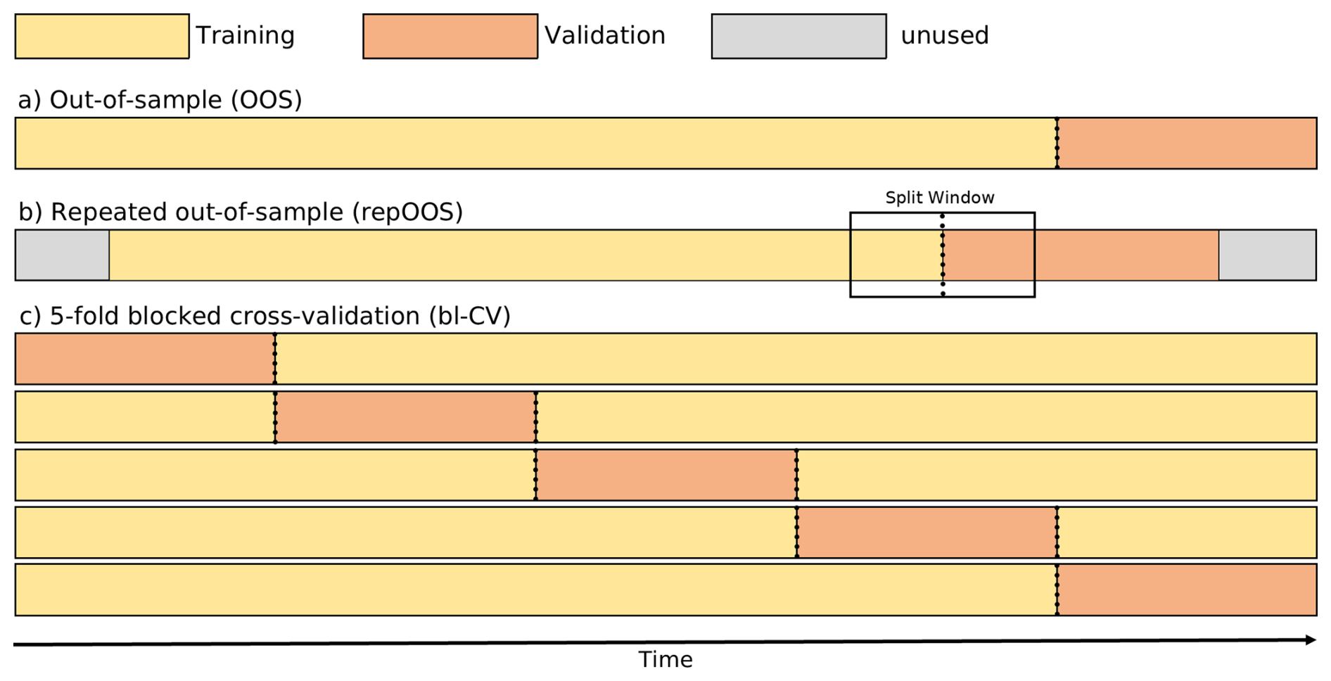
Figure 1 Schematic representation of OOS validation split (a), the splitting scheme of one repetition repOOS (b) and k-fold bl-CV (k=5) (c).

2.2 Cross-validation in time teries prediction

2.2.1 Autoregressive time series prediction

A time series is a sequential series of numerical values measured over a certain period of time:

$$\begin{array}{}\text{(1)}& \mathbf{Y}=\mathit{\{}{y}_{\mathrm{1}},y_{\mathrm{2}},y_{\mathrm{3}},\mathrm{\dots },y_n\mathit{\}},y_t\in \mathbb{R}\end{array}$$

Here, y_t is the value of Y at time t, and n is the total length of Y. Time series forecasting refers to the problem of predicting a future value from a time series Y based on a given number of past observations (lags). In the case of autoregressive modeling, a regression is performed to predict the next value of Y using the previous p lags of Y. Given a fixed number of p lags and a forecast horizon h=1, the time series is transformed as follows:

$$\begin{array}{}\text{(2)}& {\mathbf{X}}_{\mathrm{AR}}=\left[\begin{array}{cccc}{y}_{\mathrm{1}}& y_{\mathrm{2}}& \mathrm{\cdots }& y_p\\ \mathrm{⋮}& \mathrm{⋮}& \mathrm{⋮}& \mathrm{⋮}\\ y_{t-p}& y_{t-p+\mathrm{1}}& \mathrm{\cdots }& y_{t-\mathrm{1}}\\ \mathrm{⋮}& \mathrm{⋮}& \mathrm{⋮}& \mathrm{⋮}\\ y_{n-p}& y_{n-p+\mathrm{1}}& \mathrm{\cdots }& y_{n-\mathrm{1}}\end{array}\right]\mathit{y}=\left[\begin{array}{c}{y}_{p+\mathrm{1}}\\ \mathrm{⋮}\\ y_t\\ \mathrm{⋮}\\ y_n\end{array}\right]\end{array}$$

Each row of the input feature matrix X_AR represents a input feature vector formed by the past p lags of Y, while the target vector y contains the corresponding target value, which is the next observed value in the time series Y. For instance the first row of the feature matrix X_AR are therefore the input features $\mathit{\{}{y}_{\mathrm{1}},y_{\mathrm{2}},\mathrm{\dots },y_p\mathit{\}}$ and the corresponding taget value y_p+1 is in the first row of the target vector. In this form, input feature matrix X_AR and target vector y can be used for the regression to find a suitable regression function, mapping the p-dimensional input feature vectors to their respective target values.

It should be noted that this type of time series embedding leads to large overlaps between the rows of X_AR and y, which introduces statistical dependencies between the training and validation data. In particular, a target value y_t in the validation data set may already appear in the lagged input of the training data set. This violates the assumption of statistical independence required in traditional CV (Arlot and Celisse, 2010; Bergmeir and Benítez, 2012) and can lead to a distorted performance assessment, since the model already has access to target values from the validation data set during training.

This overlap problem is mitigated by modified CV approaches, such as those proposed in McQuarrie and Tsai (1998), or by hv-blocked CV presented by Racine (2000). The bl-CV described in Sect. 2.1.2 is also suitable for this dependent setting, as the overlap only occurs at the boundaries of the training and validation data. According to Bergmeir et al. (2018), however, random shuffling of assigned input-output pairs (related rows of X_AR and y) can be performed for autoregressive predictions as long as the model residuals remain serially uncorrelated, which is the case if the model is well fitted to the data.

2.2.2 Time series prediction with exogenous features

In addition to the purely autoregressive approach described in Sect. 2.2.1, feature sequences of p lags from other time series can be included (exogenous input features). The inclusion of exogenous input features can improve the accuracy of the forecast, as the target variable may be correlated with other influencing factors (Castilho, 2020).

It is also possible to discard the autoregressive approach and consider only p lags of exogenous input features. Given an exogenous time series X, which has the same length as the target time series Y (see Eq. 1):

$$\begin{array}{}\text{(3)}& \mathbf{X}=\mathit{\{}{x}_{\mathrm{1}},x_{\mathrm{2}},x_{\mathrm{3}},\mathrm{\dots },x_n\mathit{\}},x_t\in \mathbb{R}\end{array}$$

where x_t is the value of X at time t, we can construct the following input feature matrix X_EX and the corresponding target vector y, assuming a fixed number of p lags and a prediction horizon of h=1:

$$\begin{array}{}\text{(4)}& {\mathbf{X}}_{\mathrm{EX}}=\left[\begin{array}{cccc}{x}_{\mathrm{1}}& x_{\mathrm{2}}& \mathrm{\cdots }& x_p\\ \mathrm{⋮}& \mathrm{⋮}& \mathrm{⋮}& \mathrm{⋮}\\ x_{t-p}& x_{t-p+\mathrm{1}}& \mathrm{\cdots }& x_{t-\mathrm{1}}\\ \mathrm{⋮}& \mathrm{⋮}& \mathrm{⋮}& \mathrm{⋮}\\ x_{n-p}& x_{n-p+\mathrm{1}}& \mathrm{\cdots }& x_{n-\mathrm{1}}\end{array}\right]\mathit{y}=\left[\begin{array}{c}{y}_{p+\mathrm{1}}\\ \mathrm{⋮}\\ y_t\\ \mathrm{⋮}\\ y_n\end{array}\right]\end{array}$$

Contrary to the matrix X_AR described in Eq. (2) each row of the new input feature matrix X_EX contains a input feature vector formed by the past p lags of the exogenous time series X. The target vector y remains the same as in the autoregressive case, containing the corresponding target value, which is the next observed value in the time series Y. For instance the first row of the input feature matrix X_EX are therefore the input features $\mathit{\{}{x}_{\mathrm{1}},x_{\mathrm{2}},\mathrm{\dots },x_p\mathit{\}}$ and the corresponding target value y_p+1 is in the first row of the target vector y. While the structure of X_EX differs from the autoregressive input feature matrix X_AR, the target vector y is unaffected. As in the autoregressive case, the input feature matrix X_EX and the target vector y can be used for the regression to find a suitable regression function that maps the p-dimensional input feature vectors to their respective target values.

The exogenous approach uses external time series for forecasting, unlike the autoregressive approach which uses past values of the target variable as input features. This approach does not rely on potential autocorrelations within the target series, but on cross-correlations between the target variable and one or more exogenous time series. Because input features and target values originate from distinct time series, the exogenous approach is less constrained by validation techniques than the autoregressive approach. As can be seen in Eq. (4), the target values remain unique, with only consecutive values of the exogenous input features potentially appearing multiple times.

3 Experimental design

3.1 Target time series

The GWL target time series originate from groundwater monitoring wells of the State Office for the Environment Brandenburg (LfU), publicly available on the Water Information Platform of the federal state Brandenburg. Initially, 809 GWL time series covering the period from at least 1 January 1990, to 28 December 2020, were considered. Preprocessing involved aggregating on a weekly basis (Monday), applying linear interpolation for measurement gaps of up to four weeks, and imputing larger gaps (up to 52 weeks) using an iterative imputer based on Bayesian Ridge from scikit-learn (Pedregosa et al., 2011).

To capture different groundwater level dynamics, all 809 time series were classified according to their global stationarity behavior. A time series was considered weakly stationary if its mean and variance remained constant over time and its autocovariance depended only on the time lag, representing a stable system. In contrast, non-stationary time series indicate time-dependent processes, such as long-term trends or potential anthropogenic influences. Stationarity was assessed globally across the entire time series by applying two complementary statistical tests: the augmented Dickey-Fuller Unit Root (ADF) test and the Kwiatkowski-Phillips-Schmidt-Shin (KPSS) test, using default settings from the Python statsmodels package (Seabold and Perktold, 2010). A series was classified as stationary only if both tests indicated stationarity. Otherwise, it was classified as non-stationary. This analysis resulted in 294 time series being identified as weakly stationary, while 515 time series were classified as non-stationary. In the following, time series identified as weakly stationary will be referred to as stationary time series.

To reduce the computational effort, a subset of 100 GWL time series, consisting of 50 stationary and 50 non-stationary time series, was randomly selected (see Fig. 2) (Doll et al., 2026). Selecting equal numbers of both stationary and non-stationary groundwater level time series ensures that the data set includes time series with both constant means and variances and time series with changing means and variances over time, as well as long-term trends. Using this method, we were able to ensure a balanced selection of time series that reflects the full range of groundwater level variability in our data set.

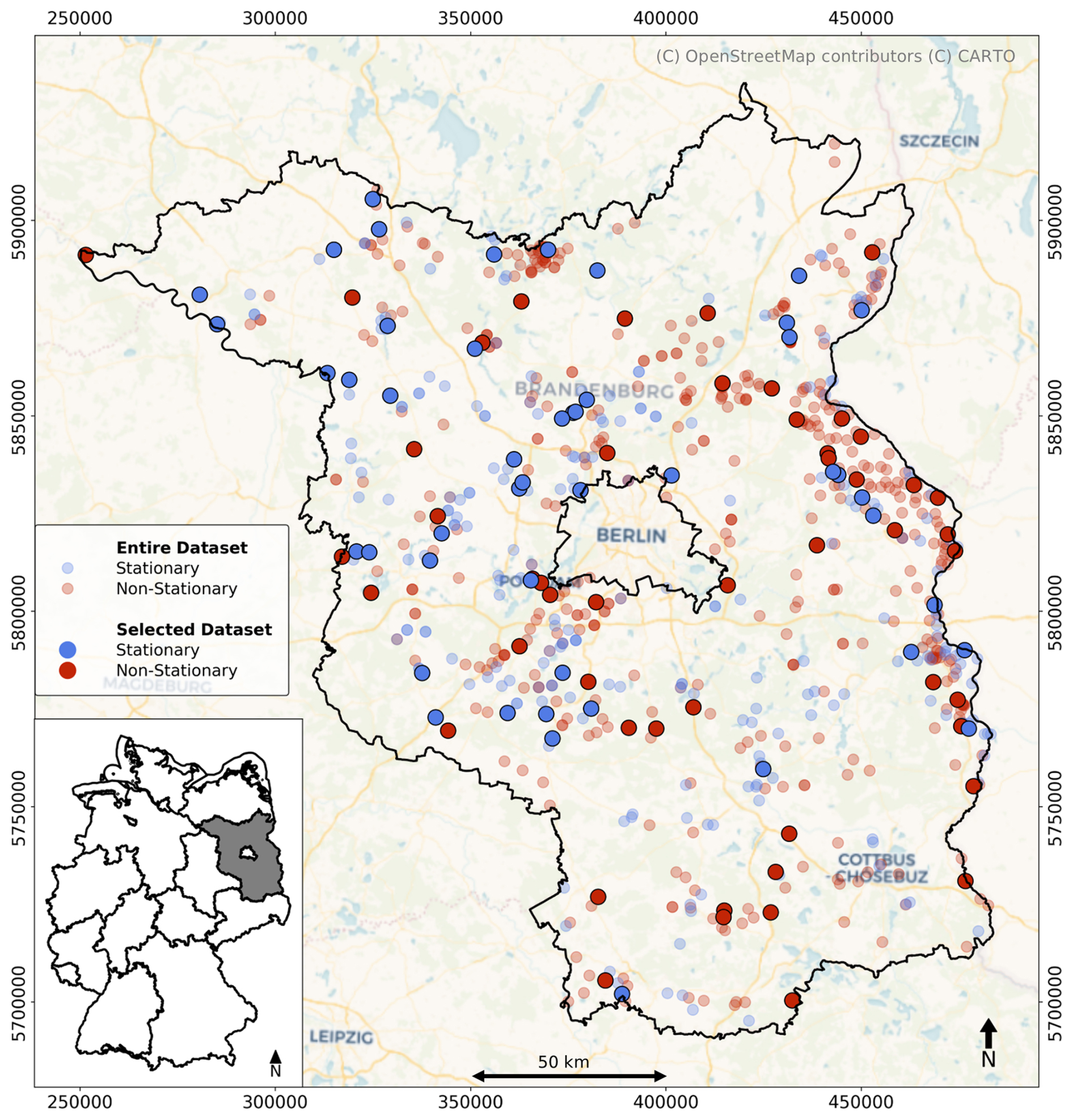
Figure 2 Map of the monitoring wells in the initial data set (809 monitoring wells) (semi-transparent colors) and the selected 100 monitoring wells used in this study (non-transparent colors). Colors indicate whether the time series are stationary (blue) or non-stationary (red).

3.2 Input time series

The meteorological parameters precipitation sum (P), mean air temperature (T), minimum air temperature (T_min), maximum air temperature (T_max) and relative humidity (rH) were used as exogenous features for the GWL forecasts. These were obtained from the publicly accessible HYRAS-DE v.5.0 dataset of the German Weather Service (DWD) (Rauthe et al., 2013; Razafimaharo et al., 2020). The HYRAS-DE v.5.0 dataset is a 5 × km² raster dataset based on meteorological observations from weather monitoring sites around Germany. For each of the selected groundwater (GW) monitoring sites, the daily HYRAS data were extracted and aggregated to weekly values (Monday). As an additional input parameter, we used a sinusoidal curve fitted to the mean air temperature (T_sin) to capture possible seasonal patterns (Wunsch et al., 2021).

3.3 Prediction task and model design

We applied a weekly sequence-to-value time series forecast, in which the future GWL (forecast horizon h=1 week) was predicted based on a sequence of p-lags (p= 52 weeks) from the exogenous meteorological input time series (this form of data embedding was explained in Sect. 2.2.2). We opted for weekly time steps, as these accurately reflect the dynamics of most aquifers and offer a good balance between data availability and the required amount of training data. The length of the meteorological input sequence was set to 52 weeks in order to map a complete annual cycle and thus fully account for seasonal influences (e.g Kunz et al., 2025).

Since we have selected weekly input and target time series from 1 January 1990 to 28 December 2020 (Sect. 3.1) and an input sequence length of 52 weeks, the predictable GWL time series begins on 31 December 1990 (first predictable value) and ends on 28 December 2020 (last value of the time series). The feature and target data were scaled to a range between 0 and 1 (MinMaxScaler; scikit-learn, Pedregosa et al., 2011) before each training run based on the corresponding training data. For the prediction task, 1D-CNN and an LSTM were implemented using Keras (Chollet, 2015). The corresponding model architectures and selected hyperparameters are presented in Fig. 3.

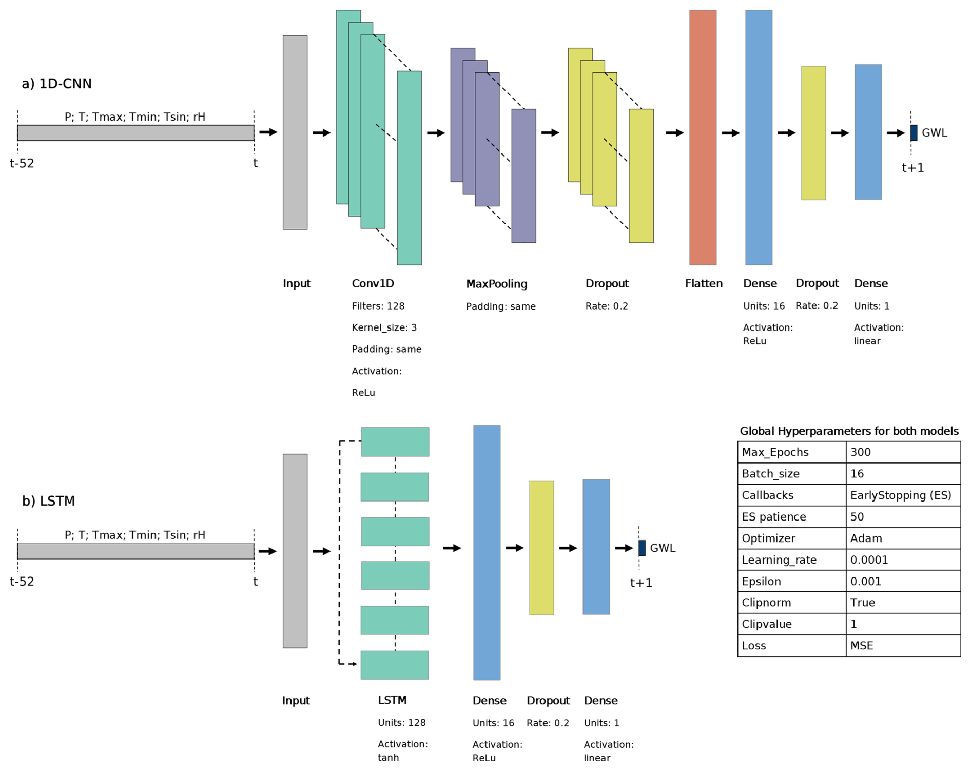
Figure 3 The model structure and the combination of the hyperparameters of the (a) 1D-CNN and the (b) LSTM model.

3.4 Training, validation and testing strategy

The objective was to assess the suitability of the three validation methods (bl-CV, repOOS, OOS) to provide the most accurate performance estimate of the actual model performance based on the unseen test data. To create this test data set, the most recent 20 % of the measurements from each GWL time series were separated from the rest of the data. This portion is referred as the out-set (Bergmeir et al., 2018). The separation of the test data was based on the standard OOS principle (Sect. 2.1.1). We chose this approach for separating the test data because our experiment was designed to simulate a real-world application where the most recent data (representative of future data) are not available during model development and parameter tuning based on the training and validation data.

The remaining 80 % of the data was used to adapt the training and to validate the prediction model. This data formed the so-called in-set (Bergmeir et al., 2018). Within this in-set, the model was trained and validated in three different ways:

• OOS (Fig. 1a). The model was trained and validated once with OOS training and validation split.

• repOOS (Fig. 1b). The model was repeatedly trained and validated using an out-of-sample training and validation split, controlled by the random choice of the split point in the split window. For the repOOS procedure, 60 % of the in-set was selected as training data and the following 10 % as validation data, according to Cerqueira et al. (2020). The available split window thus had a length of 30 %, starting after 60 % and ending at 90 % of the length of the in-set. The number of repetitions performed for this study was nrep =5.

• bl-CV (Fig. 1c). The model went through the k-folds of the k-fold bl-CV. The number of folds chosen for this study was k=5 in order to keep the validation periods as long as possible and to limit the computing effort.

In each training and validation split, an early stopping callback was set to determine the optimal number of training epochs based on the validation data and to avoid overfitting. In this way, each training and validation split provides both a prediction of the validation dataset and an estimate of the optimal number of training epochs. Since the model performance depends on the initialization of the model weights, an ensemble of 10 independent prediction models was implemented. Each model in the ensemble was initialized separately with a fixed random seed to ensure reproducibility. This resulted in five validation predictions and five optimal epoch values for the repOOS and k-fold bl-CV and in one validation prediction and one optimal epoch value for the OOS for each of the 10 ensemble members. To consolidate the results of the 10 ensemble members, the median prediction and epoch number was calculated. The exact procedure is described in detail below:

3.4.1 Procedure for OOS

• For the training and validation step, the 10 independently initialized models provided:

  • –

    10 predictions of the validation dataset,

  • –

    10 optimal number of training epochs.

• These 10 validation predictions and epoch numbers were combined into:

  • –

    A single median prediction of the validation dataset,

  • –

    A single median optimal number of epochs (Epochs_OOS).

• The root mean squared error (RMSE) between the median validation prediction and the actual measured GWL was calculated (RMSEin_OOS).

3.4.2 Procedure for repOOS (nrep = 5)

• The 10 initializations were built for each repetition, resulting in:

  • –

    10 predictions of the validation dataset,

  • –

    10 optimal numbers of training epochs,

  • –

    These 10 validation predictions and epoch numbers were combined into:

    • –

      A single median prediction of the validation dataset,

    • –

      A single median optimal number of epochs,

    • –

      The RMSE between the median validation prediction and the actual measured GWL was calculated.

• After completing the five repetitions of repOOS, this gives:

  • –

    Five RMSE (one per repetition),

  • –

    Five estimates of the optimal number of epochs (one per repetition).

• Finally, the mean of these five values was computed to obtain:

  • –

    The final repOOS in-set error (RMSEin_repOOS),

  • –

    The final repOOS epoch estimate (Epochs_repOOS).

3.4.3 Procedure for k-fold bl-CV (k=5)

• The 10 initializations were built for each fold, resulting in:

  • –

    10 predictions of the validation dataset,

  • –

    10 optimal numbers of training epochs,

  • –

    These 10 validation predictions and epoch numbers were combined into:

    • –

      A single median prediction of the validation dataset,

    • –

      A single median optimal number of epochs,

    • –

      The RMSE between the median validation prediction and the actual measured GWL was calculated.

• After completing the 5-fold bl-CV, this gives:

  • –

    Five RMSE (one per fold),

  • –

    Five estimates of the optimal number of epochs (one per fold).

• Finally, the mean of these five values was computed to obtain:

  • –

    The final bl-CV in-set error (RMSEin_bl-CV),

  • –

    The final bl-CV in-set epoch estimate (Epochs_bl-CV).

It should be noted that in this study the training and validation data split of the last fold (Fold 5) of the 5-fold bl-CV corresponds exactly to the data split used in OOS (compare Fig. 1 a and c). Therefore, the validation results from the last fold of the 5-fold bl-CV and those of the OOS are the same. The results of bl-CV include those of OOS (Fold 5) and the other four folds (Fold 1–4).

After validation at the in-set, the model is retrained with all the data from the in-set and the out-set is predicted. The number of training epochs in the out-set is determined by the optimum number of epochs determined during the corresponding validation of the in-set (Epochs_OOS, Epochs_repOOS, Epochs_bl-CV). The retraining and out-set prediction was also repeated for each of the 10 different initializations, and finally the median of the 10 ensemble predictions was calculated to obtain the final out-set prediction. Consequently, three predictions of the out-set are created. This prediction of the out-set allows the calculation of the RMSE between measured and predicted GWL of the out-set (RMSEout_OOS, RMSEout_repOOS, RMSEout_bl-CV) (see Fig. 4).

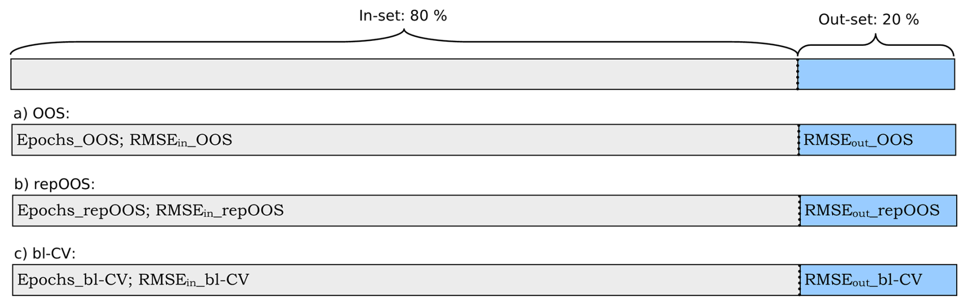
Figure 4 Illustration of the validation and testing process: Based on the validation methods in the in-set, the optimal number of training epochs (Epochs) and the model error in the in-set (RMSEin) are determined. The model is then retrained with all the data from the in-set up to the number of training epochs determined by the respective validation method. The out-set is predicted and the prediction error (RMSEout) is determined.

3.5 Performance estimation measurement

As described in Sect. 3.4, each validation procedure leads to a performance estimate RMSEin, which represents the prediction error in the in-set. The corresponding predictions of the out-set lead to the RMSEout, which represents the actual error of the model on the unseen out-set. To compare RMSEin and RMSEout, two addiational metrics were calculated following (Bergmeir et al., 2018): absolute predictive accuracy error (APAE) and predictive accuracy error (PAE).

$$\begin{array}{}\text{(5)}& \mathrm{APAE}=|{\mathrm{RMSE}}_{\mathrm{in}}-{\mathrm{RMSE}}_{\mathrm{out}}|\end{array}$$

APAE can be used to determine the absolute error between the (RMSEin) and (RMSEout). The smaller the APAE, the better the performance estimation of the corresponding validation method.

$$\begin{array}{}\text{(6)}& \mathrm{PAE}={\mathrm{RMSE}}_{\mathrm{in}}-{\mathrm{RMSE}}_{\mathrm{out}}\end{array}$$

PAE shows whether the (RMSEin) of the corresponding validation method overestimates or underestimates the (RMSEout) (bias of the performance estimate). A positive PAE means the validation method overestimated the true error (pessimistic estimate). A negative PAE indicates that the validation method underestimated the true error (optimistic estimate). As we predicted groundwater levels in meters above sea level (m a.s.l.), the RMSE, APAE, and PAE are in meters. One APAE and one PAE were calculated for each validation method, after training, validating and testing the 1D-CNN and LSTM for each time series.

4 Results and discussion

The comparison of APAE and PAE of the three performance estimation methods (Fig. 5) shows consistent patterns in terms of precision and bias for both prediction models across all 100 time series. The bl-CV yields the lowest median APAE values (1D-CNN: 0.03; LSTM: 0.03), followed by repOOS (1D-CNN: 0.05; LSTM: 0.04) and OOS (1D-CNN: 0.06; LSTM: 0.05) (Fig. 5a and b, left). The corresponding interquartile range (IQR) values are smaller for bl-CV and repOOS, while OOS shows the largest spread. The median PAE are very small, with bl-CV and repOOS exhibiting median PAE values max. 0.01, and OOS also remaining small (1D-CNN: 0.04; LSTM: 0.02).

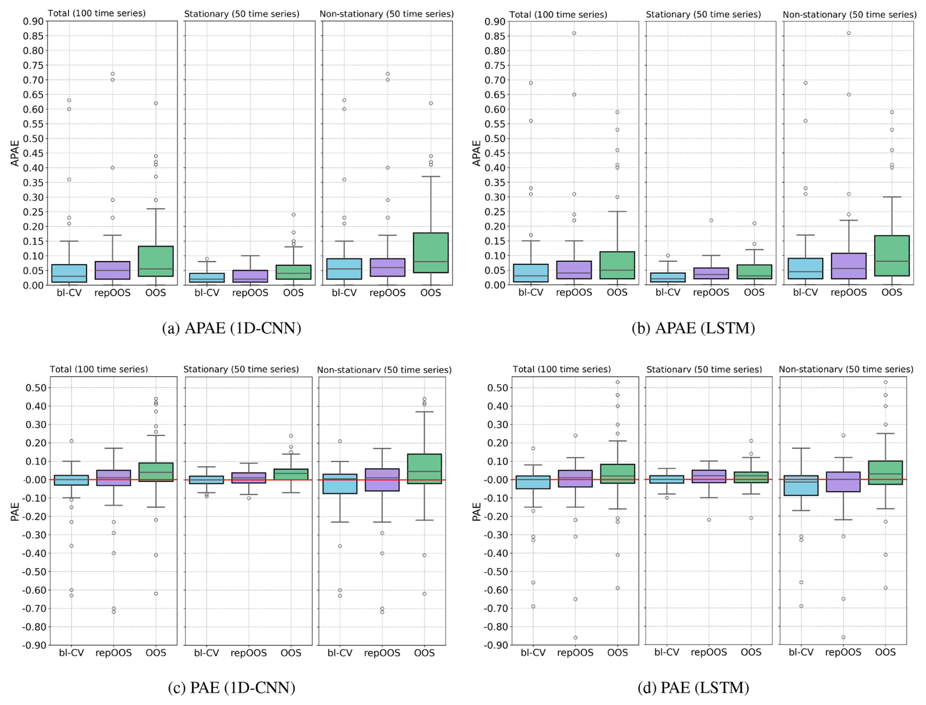
Figure 5 (a) and (b) APAE achieved per validation method across all 100 GWL time series (left), only for the 50 stationary time series (center), only for the 50 non-stationary time series (right); (c) and (d) PAE achieved per validation method across all 100 time series analyzed (left), only for the 50 stationary time series (center), only for the 50 non-stationary time series (right).

Differences become more apparent when distinguishing between stationary (n=50) and non-stationary (n=50) time series. For stationary time series, median APAE values are low for all three validation methods. For the 1D-CNN, medians are 0.02 (bl-CV), 0.02 (repOOS), and 0.04 (OOS). For the LSTM, they are 0.02 (bl-CV), 0.04 (repOOS), and 0.03 (OOS). Median PAE values for stationary time series remain small (max 0.03) across all validation methods. For non-stationary time series, median APAE and the dispersion increase. For 1D-CNN, median APAE are 0.06 (bl-CV), 0.06 (repOOS), and 0.08 (OOS). For the LSTM, they are 0.04 (bl-CV), 0.06 (repOOS), and 0.08 (OOS). Median PAE remain small but show larger dispersion. The IQR of the PAE increases for all validation methods (up to 0.16 for OOS with 1D-CNN). Overall, non-stationarity is associated with wider error distributions, indicating more variability in performance estimation across all validation approaches. It should also be emphasized that outliers in the APAE/PAE values are predominantly caused by non-stationary time series. In some cases, there are high discrepancies between RMSEin and RMSEout due to differences in the distribution of the validation and test data sets, leading to incorrect estimation of the test error (RMSEout) based on the validation error (RMSEin).

Figure 6 illustrates the relationship between RMSEin and RMSEout for stationary (left) and non-stationary (right) time series. Each point shows the RMSEin and RMSEout of one time series. The distance of the points from the diagonal line (RMSEin = RMSEout) indicates the resulting APAE. Points located above the diagonal reflect a positive deviation, indicating an overestimation of RMSEout, while points below the diagonal reflect a negative deviation, indicating an underestimation of RMSEout. A visual analysis of the scatter plots reveals that the points corresponding to OOS exhibit a greater spread around the diagonal compared to those of bl-CV and repOOS. This increased dispersion is also reflected by the larger IQR observed in the box-plots in Fig. 5, both for stationary and non-stationary time series. The scatter plot for stationary time series shows that OOS estimates RMSEout less accurately (i.e., with greater deviation from the diagonal) and more frequently overestimates it (points above the diagonal) compared to bl-CV and repOOS. These time series display slightly abnormal GWL conditions during the OOS validation period in comparison to previous years, conditions that the model fails to predict accurately. In contrast, the GWL conditions in the out-set more closely resemble those observed prior to the OOS validation period.

An analysis of the scatter plots for the non-stationary time series in Fig. 6 (right) display that the prediction errors for non-stationary time series are higher than those for stationary time series in both in-set and out-set. As a result, the prediction uncertainty is considerably greater for non-stationary time series. Moreover, Fig. 6 (right) illustrates that the spread of the data points across all validation methods is generally large and increases with higher RMSEout. This suggests that the robustness of performance estimates decreases as prediction errors increase, since larger APAE values reflect poorer model fit. The limited prediction accuracy and the resulting suboptimal performance estimates are most evident in non-stationary time series. This effect is attributable to the presence of trends or abrupt changes that cannot be adequately captured by the meteorological input sequences. A notable pattern is the tendency of OOS to overestimate high RMSEout, while bl-CV and repOOS tend to underestimate them (see Fig. 6, right).

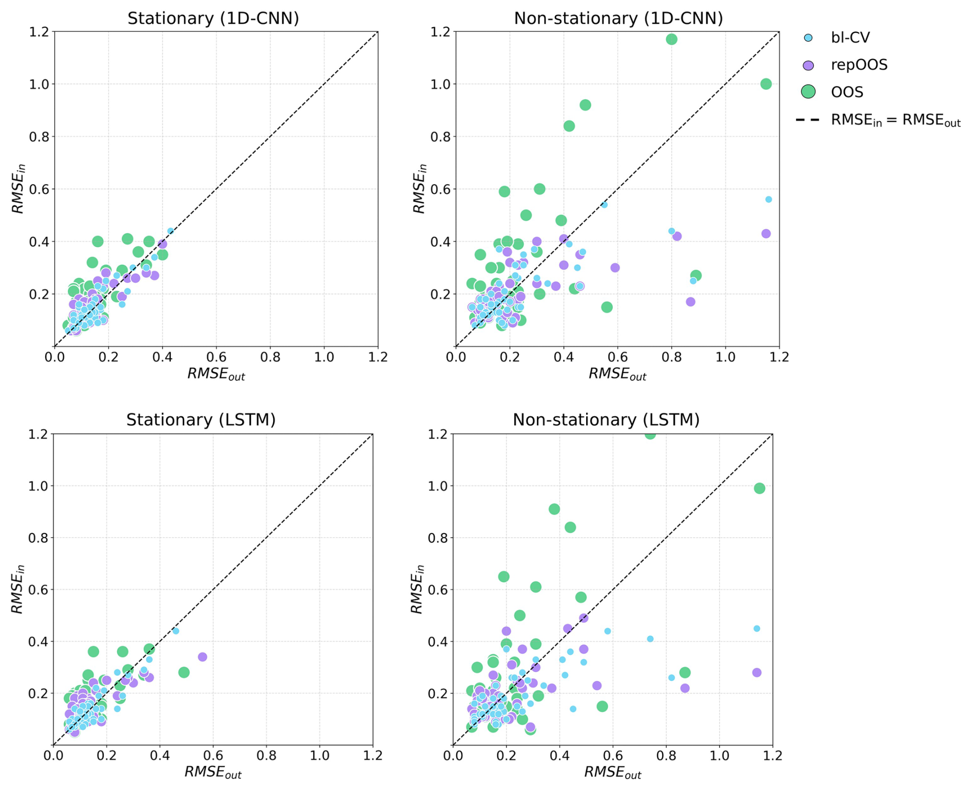
Figure 6 Point plot of the achieved RMSEin and RMSEout of the 1D-CNN (top) and the LSTM (bottom). Each point represents the RMSEin and the RMSEout of a time series validated and tested with the corresponding validation method. Left: stationary time series; Right: non-stationary time series.

Figure 7 displays the LSTM-based in-set predictions (left) with RMSEin values in the titles and the corresponding out-set predictions (right) with the respective RMSEout in the titles for the stationary time series 42.

The in-set predictions of bl-CV shows that for folds 1–4 (1991 to the beginning of 2010), the model predictions closely follow the observed groundwater levels. However, the LSTM model tends to overestimate low groundwater levels. This changes in the subsequent period (fold 5, 2010 to the end of 2014), which corresponds to the OOS validation period (see Fig. 7, center), higher groundwater levels occur more frequently and are underestimated by the model. Since the RMSE for bl-CV is calculated over all folds, the influence of the deviations in fold 5 is reduced. This results in a more robust performance estimate that is less sensitive to specific deviations (APAE: 0.03). A similar effect is observed for repOOS, where components of repetitions 3 and 5 also lie within the 2010–2014 period (see Fig. 7, bottom). However, the remaining repetitions cover different time spans, further reducing the influence of outlier periods. As a result, the average RMSE across all repetitions provides a more robust performance estimate (APAE: 0.06). In contrast, OOS relies on a single validation period, making its performance estimate highly sensitive to local anomalies in the data (APAE: 0.12). The results of the 1D-CNN model allow the same conclusions to be drawn as the LSTM results discussed above and are therefore not discussed separately. The 1D-CNN-based in-set and out-set predictions with the corresponding RMSE are shown in Fig. A1.

Figure 7 Plot of time series 42 (stationary time series, identified with global ADF and KPSS analysis). Top: LSTM based validation forecasts of the 5-folds of the bl-CV (left) and test forecasts of the bl-CV model (right); Middle: LSTM based validation forecast of the OOS validation period (left) and test predictions of the OOS model (right); Bottom: LSTM based validation predictions of the repetitions of repOOS (left) and test predictions of the repOOS model (right).

An example of validation inconsistency can be seen in Fig. 8 in time series 96. This time series shows an increase in groundwater levels from 1992 to a peak between 1994 and 1996. This is followed by a long recession period until 2008. The groundwater level then rises again within a few years, reaching the level already achieved in the mid-1990s, and then slowly falls again. The high groundwater levels of the mid-1990s and the years from 2011 to 2015 cannot be predicted well by the LSTM model, which is why the in-set predictions for these years show high deviations from the measured values. The lower groundwater levels could be explained by the meteorological input time series trends and enable a more accurate prediction of groundwater levels in these years. Averaging the RMSE of the individual validation periods for bl-CV and repOOS means that a larger amount of data from different periods within the time series are used for validation, which increases the robustness of the error estimation especially for bl-CV (APAE: 0.03 (bl-CV) and 0.09 (repOOS)). For OOS, only a single validation period is used, which carries the risk of being unrepresentative for the subsequent test period; this risk is particularly high with non-stationary time series (APAE: 0.19 (OOS)).

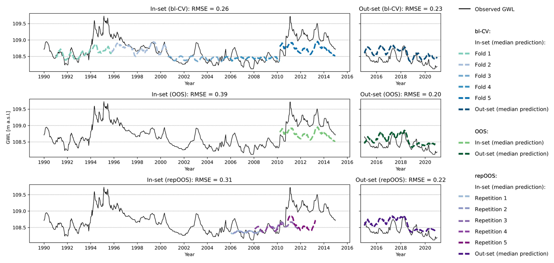
Figure 8 Plot of time series 96 (non-stationary time series, identified with global ADF and KPSS analysis). Top: LSTM based validation forecasts of the 5-folds of the bl-CV (left) and test forecasts of the bl-CV model (right); Middle: LSTM based validation forecast of the OOS validation period (left) and test predictions of the OOS model (right); Bottom: LSTM based validation predictions of the repetitions of repOOS (left) and test predictions of the repOOS model (right).

These findings underscore the need for particular care when evaluating non-stationary time series. In such cases, there is a heightened risk that the statistical properties (e.g., mean, variance) of the training, validation, and test periods differ. These discrepancies complicate both the prediction and the evaluation processes, posing greater challenges than stationary time series.

The APAE and PAE values calculated and described in this chapter are presented in numerical form in Table A1 (1D-CNN) and Table A2 (LSTM) in the Appendix. An overview of the resulting RMSEin and RMSEout values can also be found in Table A3 (1D-CNN) and Table A4.

5 Conclusions

Choosing a suitable method for performance evaluation is a key step in the development and validation of prediction models. In hydrogeological modeling, this aspect has received little attention so far. In other disciplines, validation approaches such as CV or OOS have already been extensively investigated with regard to their suitability for evaluating autoregressive time series forecasting (e.g. Bergmeir and Benítez, 2011, 2012; Bergmeir et al., 2014, 2018; Cerqueira et al., 2020). Several of these studies show that bl-CV provides the most robust and accurate performance estimates for stationary time series (Bergmeir and Benítez, 2011, 2012; Bergmeir et al., 2014; Cerqueira et al., 2020), while Cerqueira et al. (2020) recommended repOOS for non-stationary time series.

In hydrogeology, however, long-term forecasts are often required. This reduces the relevance of autoregressive models and increases the importance of purely exogenous input data, such as meteorological drivers, which are available as climate forecasts. The results of existing studies on autoregressive models can therefore only be applied to a limited extent to the prediction of (GWL) using exogenous variables. The present study addresses this gap by applying three validation methods (bl-CV, repOOS, and OOS) for the prediction of 100 GWL time series (50 stationary, 50 non-stationary) based on meteorological input data (precipitation, air temperature [mean, minimum, maximum], relative humidity, and a seasonal temperature sine curve). The GWL for the coming week was predicted from a 52-week meteorological input sequence. To evaluate the validation methods, APAE and PAE were calculated according to Bergmeir et al. (2018).

The results show that bl-CV provides the most accurate and robust performance estimates, both across all 100 time series and separately for stationary and non-stationary series. repOOS follows in second place, while OOS has the most unreliable estimates. The higher robustness of bl-CV and repOOS can be attributed to the fact that both methods take multiple validation periods into account, whereas OOS uses only a single period and is therefore more susceptible to outliers. Although a direct comparison with studies on autoregressive forecasts is only possible to a limited extent, the results confirm the findings of Bergmeir and Benítez (2011), Bergmeir and Benítez (2012), Bergmeir et al. (2014) and Cerqueira et al. (2020), according to which bl-CV is a suitable choice for stationary time series. For non-stationary time series, however, the results differ from the autoregressive case in Cerqueira et al. (2020): Contrary to what is recommended there, bl-CV proves to be more accurate and robust for performance estimation than repOOS in our study. Furthermore, the results suggest that predictions from stationary GWL time series led to more robust forecasts and more reliable performance estimates. In contrast, non-stationary time series were associated with higher prediction errors and increased uncertainty in the performance assessment of all investigated validation methods. The stationary time series GWL showed less complex patterns, which could be captured more effectively by meteorological input variables and consequently predicted more accurately by the 1D-CNN and LSTM models across the entire time series. Non-stationary time series, on the other hand, exhibited more complex, time-dependent structures, which made accurate predictions over different periods within the time series and thus also correct performance estimation more difficult. These more difficult conditions require particular caution when interpreting the validation results. Even taking test errors into account, a technical evaluation is necessary to ensure that validation and test periods are indeed representative. For future studies, especially in the case of non-stationary time series, it may be useful to deviate from the consecutive validation approaches commonly used in time series forecasting and instead investigate deterministic data splitting methods. Such methods are recommended by Zheng et al. (2022) for hydrological precipitation-runoff models to ensure the consistency of the statistical distribution in the individual sub-datasets. Although bl-CV and repOOS partially compensate for distribution differences between training, validation, and test data by selecting and positioning several validation periods, a discrepancy between the final test period and the preceding periods may still remain in non-stationary series. Selecting sufficiently large and representative validation and test periods can mitigate the influence of anomalous periods and improve the validity of performance estimates, ultimately supporting more informed and resilient groundwater management decisions.

Appendix A

Table A1 Descriptive statistics for APAE and PAE (total, stationary, non-stationary) for 1D-CNN.

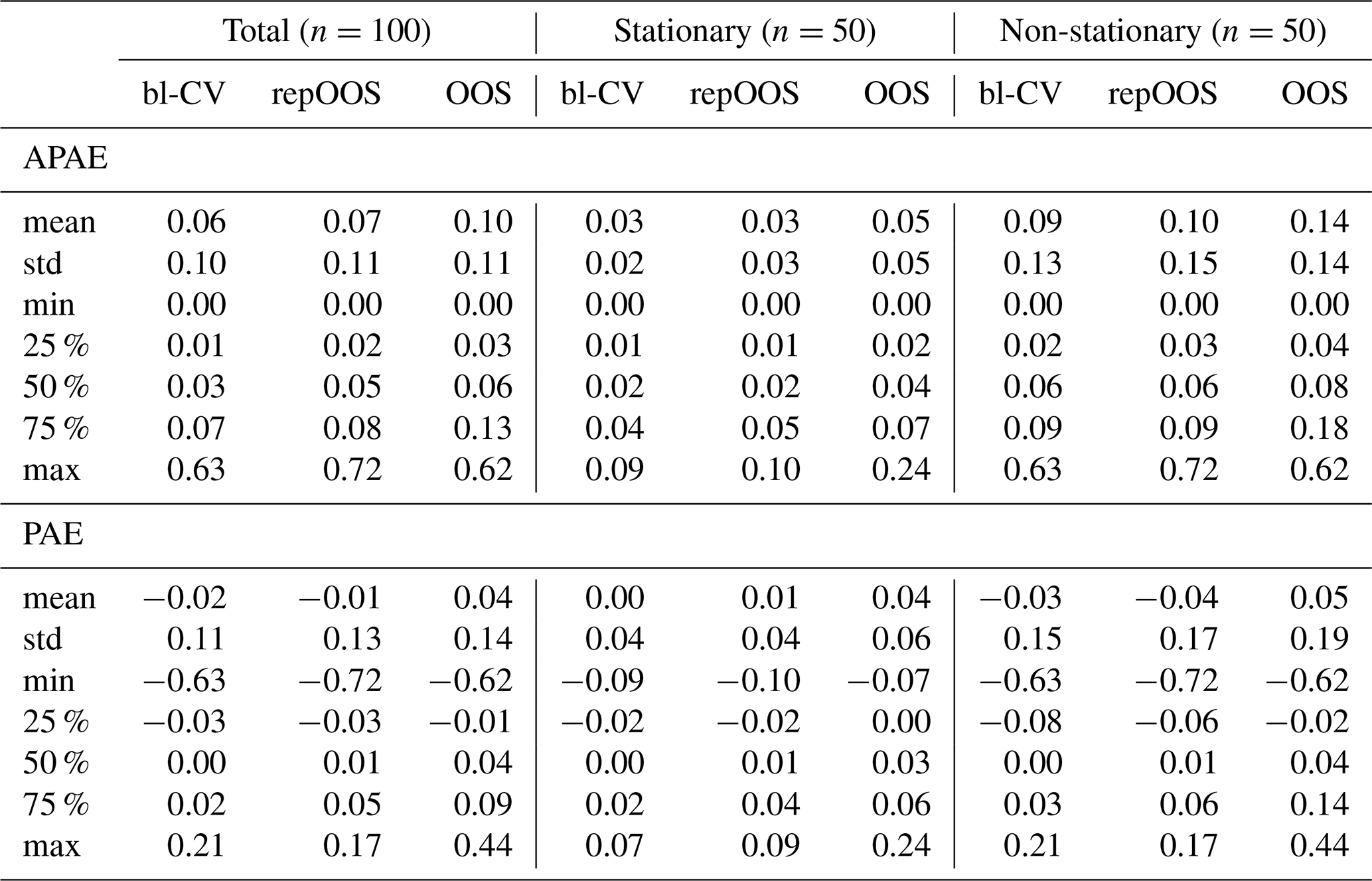
Table A2 Descriptive statistics for APAE and PAE (total, stationary, non-stationary) for LSTM.

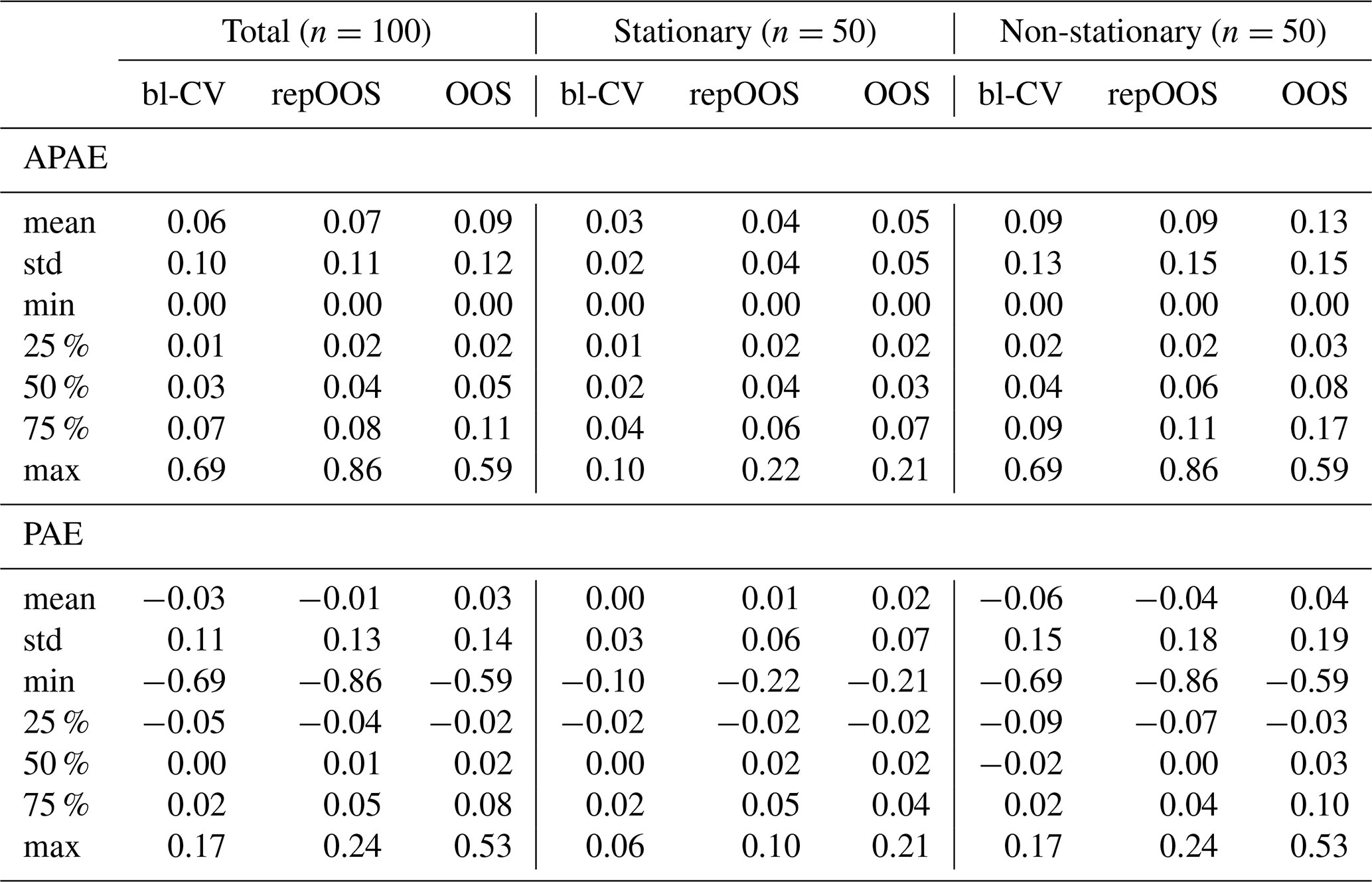
Table A3 Descriptive statistics for RMSE (in-set and out-set, total, stationary, non-stationary) for 1D-CNN.

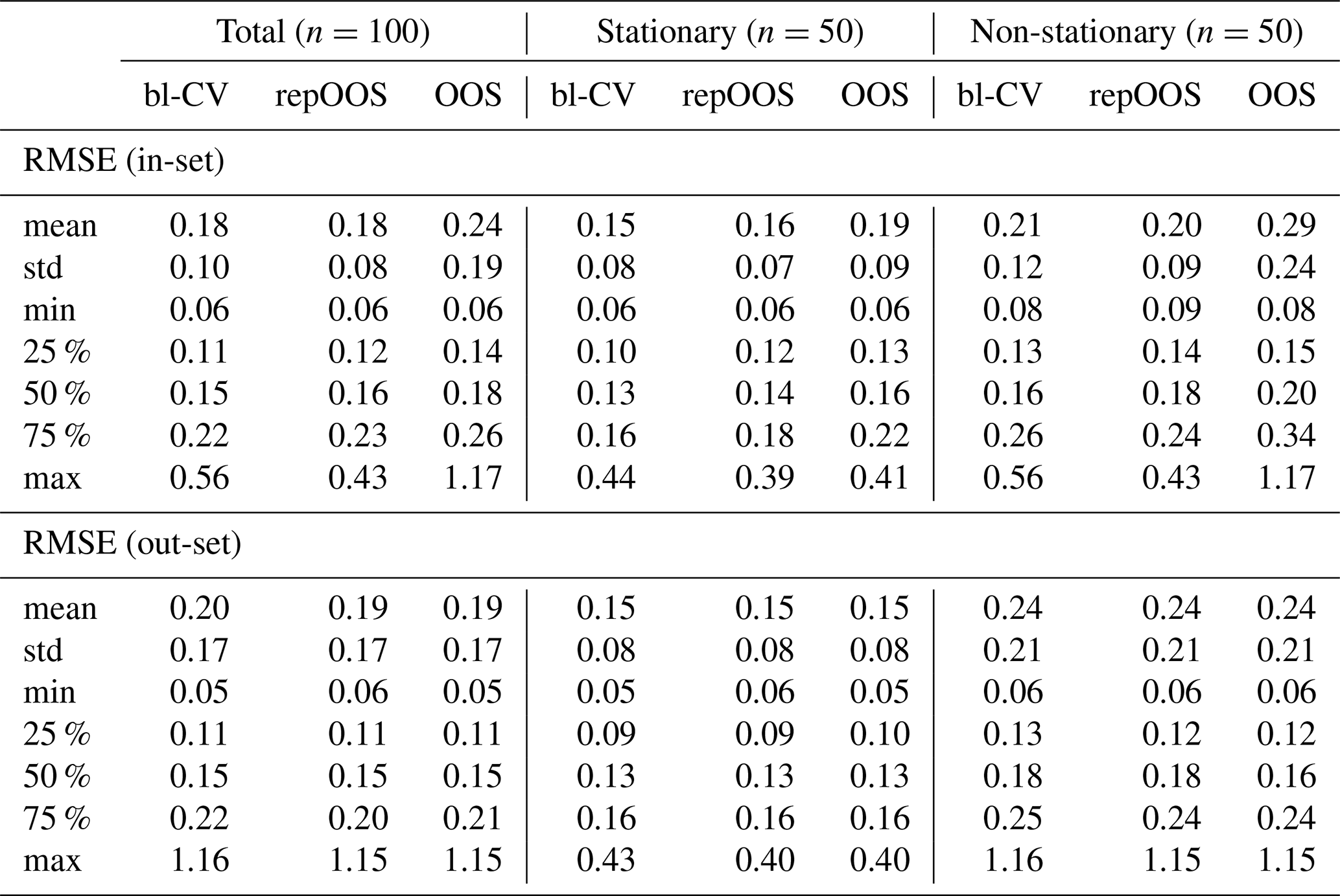
Table A4 Descriptive statistics for RMSE (in-set and out-set, total, stationary, non-stationary) for LSTM.

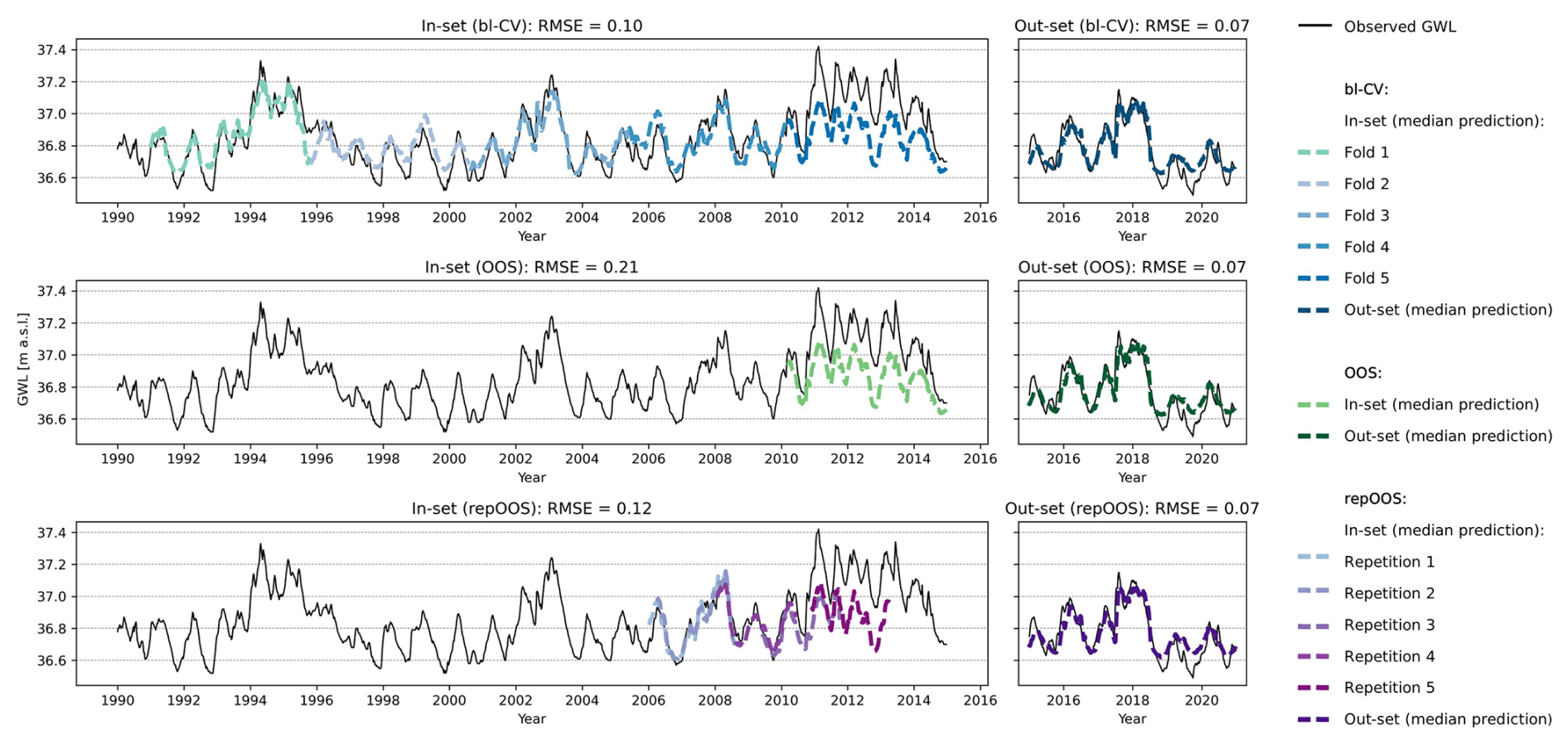
Figure A1 Plot of time series 42 (stationary time series, identified with global ADF and KPSS). Top: 1D-CNN based validation forecasts of the 5-folds of the bl-CV (left) and test forecasts of the bl-CV model (right); Middle: 1D-CNN based validation forecast of the OOS validation period (left) and test predictions of the OOS model (right); Bottom: 1D-CNN based validation predictions of the repetitions of repOOS (left) and test predictions of the repOOS model (right).

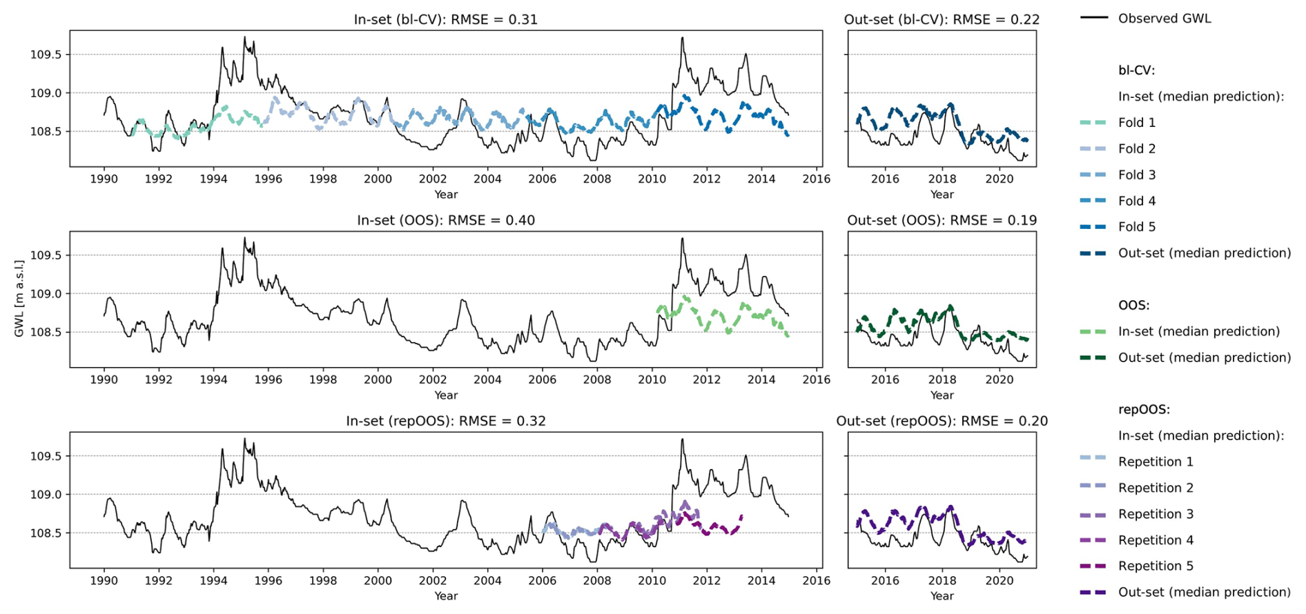
Figure A2 Plot of time series 96 (non-stationary time series, identified with global ADF and KPSS). Top: 1D-CNN based validation forecasts of the 5-folds of the bl-CV (left) and test forecasts of the bl-CV model (right); Middle: 1D-CNN based validation forecast of the OOS validation period (left) and test predictions of the OOS model (right); Bottom: 1D-CNN based validation predictions of the repetitions of repOOS (left) and test predictions of the repOOS model (right).

Appendix B: Nomenclature

1D-CNN	one-dimensional convolutional neural
	network
ADF	augmented Dickey-Fuller Unit Root
AI	artificial intelligence
ANN	artificial neural networks
APAE	absolute predictive accuracy error
bl-CV	blocked cross-validation
CNN	convolutional neural network
CV	cross-validation
DL	deep learning
DWD	German Weather Service
GRU	gated recurrent unit
GW	groundwater
GWL	groundwater level
HYRAS-DE	hydro-meteorological gridded data
	for Germany
IQR	interquartile range
KPSS	Kwiatkowski-Phillips-Schmidt-Shin
LfU	State Office for the Environment
	Brandenburg
LSTM	long-short-term memory
m a.s.l.	meters above sea level
ML	machine learning
OOS	out-of-sample validation
P	precipitation sum
PAE	predictive accuracy error
repOOS	repeated out-of-sample validation
rH	relative humidity
RMSE	root mean squared error
T	mean air temperature
Tmax	maximum air temperature
Tmin	minimum air temperature
Tsin	sinusoidal curve fitted to the mean
	air temperature