Deep learning representation of the aerosol size distribution

Aerosols influence Earth's radiative balance via the scattering and absorbing of solar radiation, affect cloud formation, and play important roles on precipitation, ocean seeding and human health. Accurate modeling of these effects requires knowledge of the chemical composition and size distribution of aerosol particles present in the atmosphere. Computationally intensive applications like remote sensing and weather forecasting commonly use simplified representations of aerosol microphysics, prescribing the aerosol size distribution (ASD), introducing uncertainty in climate predictions and aerosol retrievals. In this work, we develop a neural network model, MAMnet, to predict the ASD and mixing state for seven lognormal modes based on the bulk aerosol mass and the meteorological state. MAMnet is designed to operate with outputs from single-moment, mass-based aerosol schemes, making it compatible with existing models. We demonstrate that MAMnet can accurately reproduce the output of a two-moment modal aerosol scheme, and also agrees well with field measurements when driven by reanalysis data. Our model paves the way to improve the representation of aerosols in atmospheric models while maintaining the versatility and efficiency required in large scale applications.

1 Introduction

Aerosols play a crucial role in the Earth's system by influencing radiative forcing (Forster et al., 2007; Bender, 2020), cloud formation and lifetime (Christensen et al., 2020), and precipitation patterns (Stier et al., 2024). Aerosol particle size and composition determine their atmospheric lifetime (Seinfeld and Pandis, 2016), impact on human health (Arfin et al., 2023), long range transport (Uno et al., 2009), and their ability to become cloud droplets and ice crystals (Seinfeld et al., 2016). The size and composition of atmospheric aerosols are critical parameters determining the concentration of cloud condensation nuclei (CCN) in the atmosphere (Seinfeld and Pandis, 2016). Understanding the distribution and composition of atmospheric aerosols is thus essential for accurate climate and weather simulations (Seinfeld et al., 2016).

The ASD and mixing state are at the center of the ability of climate models to accurately simulate the transport and chemical evolution of aerosol species (Aquila et al., 2011; Bender et al., 2019). Variability in the representation of the ASD among models has been shown to drive large differences in cloud droplet number concentration and aerosol–cloud radiative forcing (Virtanen et al., 2025). Explicitly resolving the ASD improves the representation of nucleation, condensation, and coagulation processes (Zhou et al., 2018), and it is critical for realistically simulating scavenging within clouds, as smaller particles are less efficiently removed than larger ones, affecting global particle number concentrations by up to 20 % (Pierce et al., 2015). It has been shown that models that resolve particle-level mixing state and size better represent CCN activity, aerosol aging, and radiative properties (Riemer et al., 2019).

Atmospheric models represent the ASD using approximations with different degrees of sophistication. The bulk mass approach predicts the transport and evolution of aerosols by tracking the mass concentration of individual chemical species (Jones et al., 1994; Langner and Rodhe, 1991; Ginoux et al., 2001; Chin et al., 2000). Each particle is assumed to consist of a single chemical component or their surrogate (Riemer et al., 2019). Because each species is typically represented by a single prognostic variable, the bulk approach is not designed to resolve the ASD or the mixing state, which are often prescribed from climatological data. However, due to their low computational cost, bulk schemes are well suited for data assimilation (Randles et al., 2017) and are widely used in forecasting systems, satellite retrieval algorithms, and reanalysis products (Chu et al., 2002; Gelaro et al., 2017; Inness et al., 2019). For example, aerosol transport in the MERRA-2 climate reanalysis (Gelaro et al., 2017; Randles et al., 2017) is based on the Goddard Chemistry, Aerosol, Radiation, and Transport model (GOCART) (Colarco et al., 2010b). GOCART is a bulk aerosol scheme that explicitly calculates the mass of major species, i.e., dust, black carbon, organic material, sea salt, and sulfate, using an externally mixed representation.

In contrast to bulk methods, modal aerosol schemes estimate both the number concentration and mass of atmospheric aerosol, approximating the ASD as the combination of overlapping populations, termed “modes”, each typically assumed internally-mixed, and following a log-normal distribution with prescribed geometric standard deviation (e.g., Whitby and McMurry, 1997; Wilson et al., 2001; Stier et al., 2005; Mann et al., 2010; Liu et al., 2012). Because they predict the number concentration and mass independently, modal schemes can better resolve the composition of aerosol species, particularly when several subpopulations are used (Riemer et al., 2019). More sophisticated aerosol schemes either compute additional moments of the ASD (Zhang et al., 2020), explicitly resolve it using a binned approach (e.g., Adams and Seinfeld, 2002), or represent it on a particle-by-particle basis (Riemer et al., 2019). While these models provide the most physically consistent representation of the ASD, they are often too computationally expensive for operational forecasting and long-term climate simulations.

In computationally intensive applications and satellite retrievals it is desirable to maintain the efficiency and simplicity of the bulk schemes. However, key processes such as nucleation, coagulation, scavenging, and activation, as well as aerosol radiative properties, are highly sensitive to particle size, requiring the explicit representation of the ASD (Seinfeld and Pandis, 2016). A common approach to address this is to prescribe a global mean ASD (e.g., Remer et al., 2005; Barahona et al., 2014; Inness et al., 2019; Block et al., 2024). Yet, aerosol size and composition vary substantially across time and space, influenced by both meteorological conditions and natural and anthropogenic sources. As a result, a fixed global ASD can only approximate the actual, locally varying distribution, potentially introducing biases in the simulation of aerosol–radiation and aerosol–cloud interactions.

To address these challenges, there is growing interest in leveraging machine learning (ML) techniques to develop more efficient and accurate aerosol models (e.g.,  Rasp et al., 2018; Gong et al., 2022; Silva et al., 2021; Harder et al., 2022). ML models, can in principle capture complex nonlinear relationships between aerosol properties and environmental variables with reduced computational costs. For example, Harder et al. (2022) developed a surrogate of the Modal Aerosol Module (MAM7; Liu et al., 2012) to predict the mass and number tendencies of aerosol species, with the aim to improve computational performance. The emulator replaces computationally intensive parts of MAM7, however does not map the ASD to the mass of the aerosol species, a requirement to many assimilation and remote sensing algorithms (Randles et al., 2017; Buchard et al., 2017). Other work also have sought to use ML to predict the ASD from bulk aerosol mass, focusing on specific species or its effect on cloud formation (Nair et al., 2021; Zhu et al., 2023).

Here we present a novel ML-based approach for predicting the ASD and aerosol mixing state in atmospheric models that run bulk aerosol schemes. This is accomplished by developing a ML-based parameterization that emulates the ASD predicted by the MAM7 model, using as input the total mass of aerosol species from relatively fast single-moment bulk aerosol models like GOCART. By combining the strengths of machine learning and physical principles, the parameterization maps the bulk mass model into the ASD that would be predicted by the modal approach, enhancing the former. Our method offers a promising avenue for advancing aerosol representation in climate predictions, data assimilation and remote sensing applications.

2 Methods and Data

We developed a neural network (NN) termed “MAMnet”, to estimate the ASD using as input the total mass of aerosol species, air density and temperature. This minimal set of inputs ensures that the neural network remains independent of the host model, since including additional meteorological inputs like wind speed and humidity, would introduce sensitivity to model-specific parameterizations. It also makes MAMnet suitable for applications involving satellite aerosol retrievals, where only a limited set of atmospheric variables is typically available. This approach is supported by previous studies showing that the conversion between aerosol mass and number concentrations can be reasonably approximated using spatially varying, but prescribed, ASDs (e.g., Remer et al., 2005; Inness et al., 2019; Block et al., 2024), suggesting that such relationships can be effectively learned by a neural network. MAMnet was trained on simulated data using the MAM7 model implemented on the NASA's Global Earth Observing System (GEOS). This section details the modeling components as well as the development and evaluation approach of the NN.

2.1 Modeling components

The NASA Goddard Earth Observing System (GEOS), consists of a set of components that numerically represent different aspects of the Earth system (atmosphere, ocean, land, sea-ice, and chemistry), coupled following the Earth System Modeling Framework (https://gmao.gsfc.nasa.gov/GEOS_systems/, last access: 23 March 2026). In GEOS-AGCM configuration, atmospheric transport of water vapor, condensate and other tracers, and associated land-atmosphere exchanges, is computed explicitly, whereas sea-ice and sea surface temperature (SST) are prescribed as time-dependent boundary conditions (Reynolds et al., 2002; Rienecker et al., 2008). Cloud microphysics in the operational version of GEOS uses a single moment microphysics scheme for short-term weather forecast (Molod et al., 2015), and a two-moment cloud scheme in subseasonal and seasonal prediction (Barahona et al., 2014; Molod et al., 2020). GEOS constitutes the modeling base of MERRA-2 (Modern Era Retrospective analysis for Research and Applications, version 2), the first multidecadal reanalysis to integrate both aerosol and meteorological observations (Gelaro et al., 2017; Randles et al., 2017). In MERRA-2 aerosol fields are described using GOCART. Aerosols are interactive and radiatively active, hence MERRA-2 has a representation of the aerosol direct effect. Aerosol assimilation uses the Goddard Aerosol Assimilation System (GAAS), and the overall assimilation cycle is controlled by the meteorology.

2.1.1 Aerosol transport schemes

GEOS implements two aerosol schemes to interactively calculate the evolution of aerosol and gaseous tracers. Both include parameterized representation of aerosol formation, growth, aging and wet removal, and differ in their treatment of the ASD and mixing state. GOCART (Chin et al., 2000; Colarco et al., 2010a) is used operationally on weather forecast and data assimilation applications. GOCART is a mass-based aerosol model that explicitly calculates the transport and evolution of dust, black carbon, organic material, sea salt, and sulfate. Aerosol species are assumed externally mixed. Dust and sea salt are represented in five mass bins of different sizes whereas a single bin is assumed for other species. The ASD for each bin is prescribed as a lognormal distribution. Both organics (primary and secondary organic matter) and black carbon are split into hydrophilic and hydrophobic components. Dust and sea salt emissions are prognostic whereas sulfate and biomass burning emissions are obtained from the MERRA-2 dataset (Colarco et al., 2010a; Randles et al., 2017).

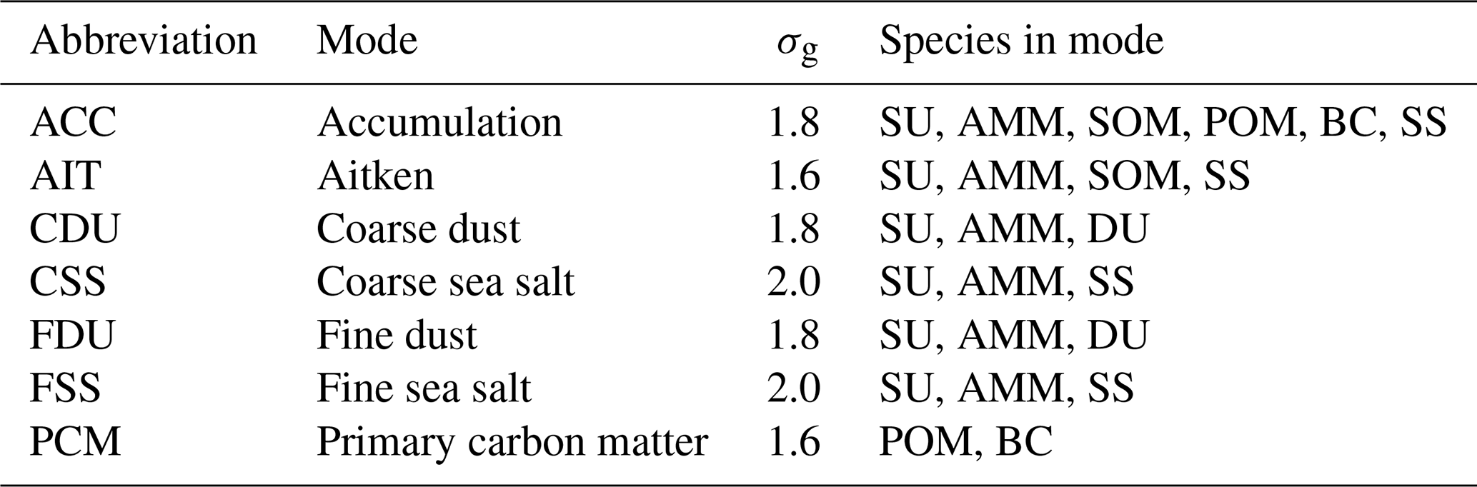
GEOS also implements the MAM7 model (Liu et al., 2012), as an alternative aerosol scheme for research applications. MAM7 is a modal aerosol scheme that predicts the mass and number concentration of Aitken (AIT), accumulation (ACC), primary carbon (PCM), fine dust (FDU) and sea salt (FSS), and coarse dust (CDU) and sea salt (CSS) aerosol modes. The aerosol representation is internally mixed with aerosol species and modal composition as detailed in Tables 1 and 2. The total number of simulated tracers in MAM7 is 31: 24 modal mass components and seven aerosol number concentrations. The size distributions for each mode is assumed to follow a lognormal distribution, with geometric mean diameter computed diagnostically and prescribed geometric standard deviation for each mode (Liu et al., 2012).

Table 1 Aerosol species considered in this work; κ is the hygroscopicity parameter (Kreidenweis et al., 2005).

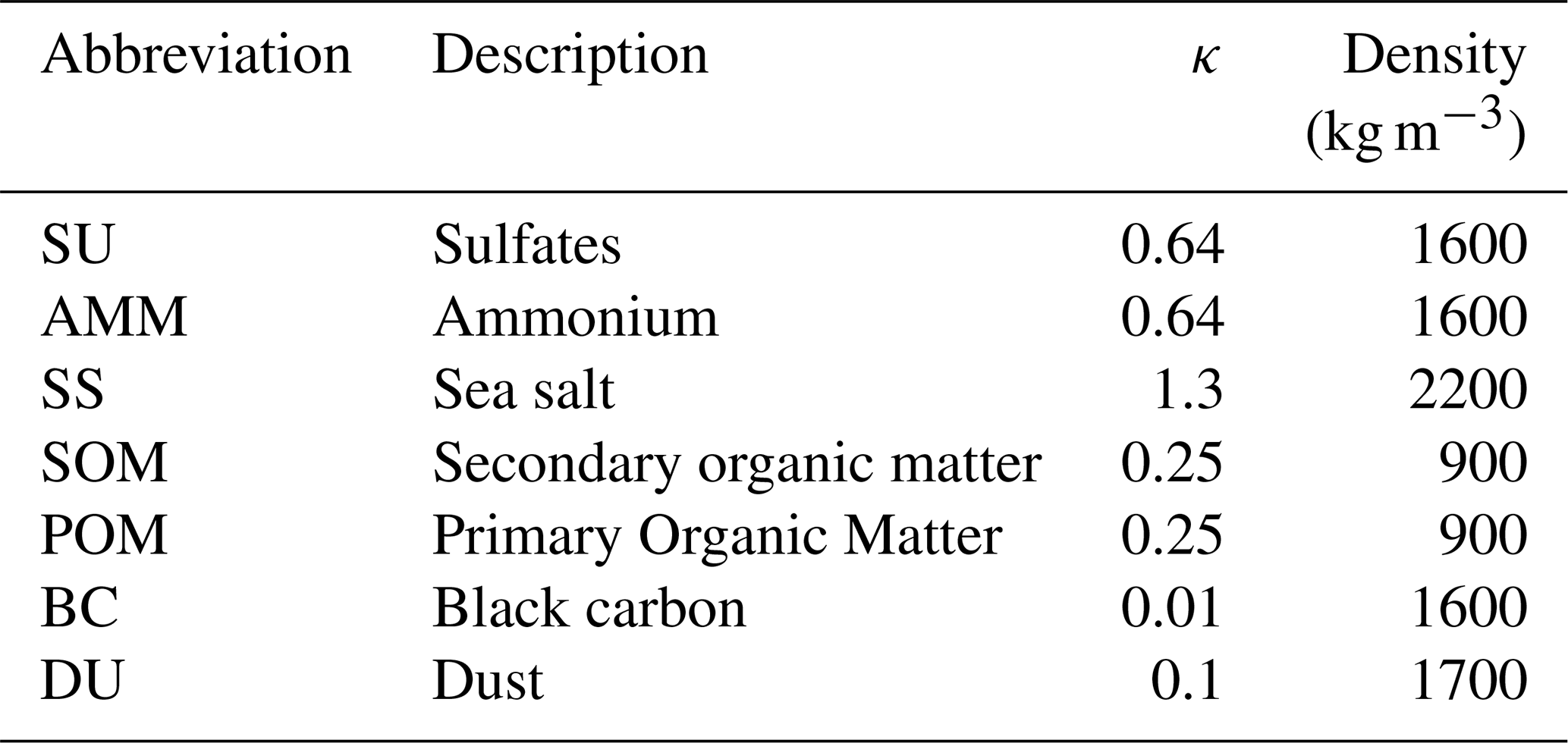
Table 2 Aerosol modes predicted by MAM7 and MAMnet; σ_g is the geometric standard deviation.

2.2 Development of the deep learning model

We built a neural network, termed “MAMnet”, to estimate the aerosol number concentration and composition emulating the output of the MAM7 model (Table 2), using as input the total mass mixing ratios for dust, sulfates, organics, black carbon and sea salt, and the atmospheric state (temperature, T and air density, ρ_air), for a total of 31 predicted tracers as shown in Fig. 1. MAMnet is intended to map the simulated aerosol mass across species into a 7-modal ASD, rather than to fully emulate MAM7. This is arguably a simpler task than emulating the full range of aerosol processes represented in MAM7, since the aerosol mass fields used as input already encapsulate the integrated effects of meteorology, clouds, as well as trends in aerosol emissions. The mass-number relationship on the other hand is not expected to depend strongly on such factors, since it many cases it can be approximated to some degree using prescribed formulations for the ASD (McCoy et al., 2017). This section describes the development of the NN.

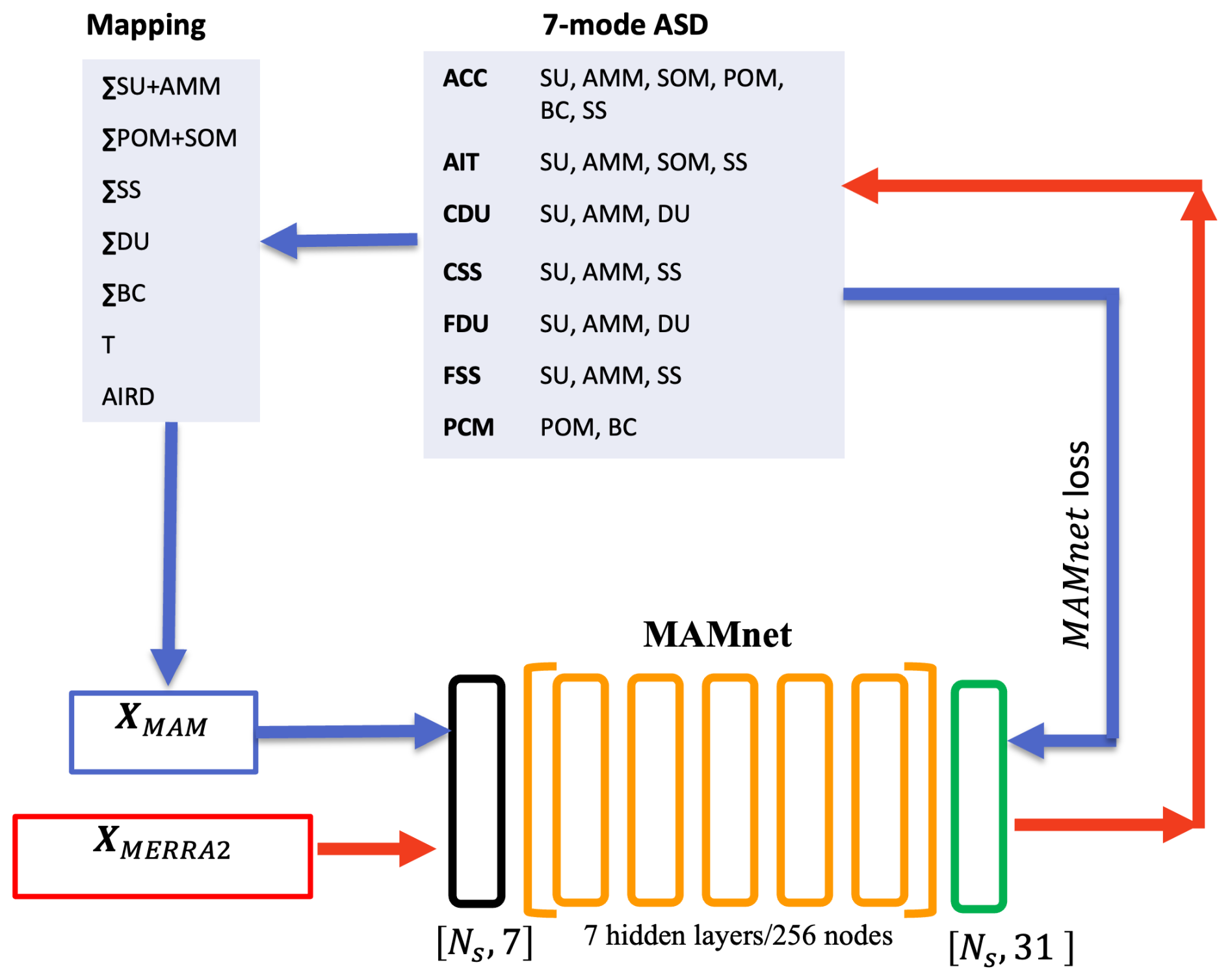
Figure 1 Neural network development workflow. Blue arrows represent the training steps, while red arrows correspond to the inference process. During training, the “mapping” step aggregates aerosol species across modes from the MAM7 output to construct the input X_MAM. The MAM7 output is then used to calculate the MAMnet loss (calculated as the minimum mean square difference between the model prediction and the MAM7 fields). During inference, input from MERRA-2 is used to predict the aerosol size distribution and mixing state. MAMnet consists of a single input layer (black), seven hidden layers (orange), and one output layer (green). T and AIRD represent the temperature and air density, respectively. N_s is the number of samples.

2.2.1 Data generation

The AGCM configuration of GEOS, running MAM7 (referred to as “GEOS+MAM7”), was used to develop a robust dataset to train the neural network. We ran a 5-year simulation (2001–2006) at 1° horizontal resolution and 72 vertical levels (from the surface to 0.01 hPa), with diurnal, instantaneous outputs at UTC 09:00:00 and 21:00:00. Temperature and horizontal winds were “replayed” to MERRA-2. The replay technique is a form of nudging that combines analysis increments with the model results every six hours, at each model grid point, to correct the model state (Takacs et al., 2018). This ensures that the simulation reproduces the observed meteorological state. Aerosol mass however evolves freely from observational constraints.

To construct the training dataset, we randomly selected 25 unique output files (without replacement) from the years 2001–2005. An additional 10 unique files were used as validation data to compute the loss during training. Each file represents global instantaneous output from the GEOS+MAM7 model. Although the validation data are not used to update the network parameters, the validation loss informs optimization choices (e.g., early stopping and hyperparameter selection) and is therefore considered part of the training process. For testing, we used 5 separate output files from the year 2006, which was not included in either the training or validation stages, ensuring a fully independent evaluation set.

Each grid cell in the GEOS+MAM7 output is treated as an independent training example, resulting in a large volume of data: with N_time=25 timestamps, N_lev=72 vertical levels, N_lat=181 latitudes, and N_lon=360 longitudes, the training set contains over 100 million samples. The samples are randomly shuffled in time and space prior to training. This single-cell approach makes the parameterization resolution-independent, facilitating integration into atmospheric models with varying grid resolutions. It also ensures broad coverage of physically plausible combinations of aerosol mass and number. Although this approach omits spatial or vertical correlations, the mass-number relationship depends primarily on the relative abundance of species within a given grid cell. This was tested by using using a full-column input structure, which resulted in no significant gain in accuracy (not shown).

To balance data volume and temporal representativeness, we sampled at 12 h intervals, which allows the network to capture differences between day and night while maximizing the number of training samples. Higher-frequency sampling could better resolve the diurnal cycle, but this comes at the cost of fewer training time steps due to memory limitations. This is not expected to be critical as the relationship between aerosol mass and number is expected to exhibit weaker diurnal variability than mass itself, which would be already resolved by the host model.

We combined the internally-mixed, modal mass components parameterized by MAM7 across 5 different species including sulfate, ammonium, sea salt, dust, primary and secondary organic matter, and black carbon (Table 1 and Fig. 1) to derive the total mass mixing ratios for the input features. Neither MERRA-2 nor the current implementation of MAM7 in GEOS include nitrate aerosol species. The mass input variables were first log₁₀-transformed, and the resulting values were then standardized by computing Z-scores using the global mean and standard deviation across all levels. Temperature and air density were also standardized using their global mean and standard deviation. Statistics used for normalization were calculated using 100 random instantaneous output files not used during training. Target variables included the mass of each of the MAM7 species and the number concentration for each mode. Because aerosol mass and number concentration vary over several orders of magnitude, we log₁₀-transformed the targets, and filtered out values less than minimum threshold values, 10⁻²⁰ µg kg ⁻¹ and 10⁻⁴ mg⁻¹ for mass and number, respectively, prior to training. Values below these thresholds are held constant and therefore do not contribute to the gradient. During testing, points below the thresholds are masked. All metrics are computed in logarithmic space.

The modal aerosol dry diameter (hereafter D_pg) was not directly included as a target of MAMnet, and it is not part of the loss function. Instead it was used to check for mass conservation, that is, matching the predicted D_pg against the target values indicates that the mass and number concentration remain consistent in the prediction. D_pg was derived for each ith mode in the form (Seinfeld and Pandis, 2016),

$$\begin{array}{}\text{(1)}& D_{\mathrm{pg},i}={\left({\displaystyle \frac{\mathrm{6}}{\mathit{\pi }{N}_i}}\sum _{j=\mathrm{1}}^{N_{\mathrm{sp},\mathrm{i}}}{\displaystyle \frac{M_{j,i}}{{\mathit{\rho }}_{j,i}}}\right)}^{\mathrm{1}/\mathrm{3}}\exp \left(-{\displaystyle \frac{\mathrm{3}{\ln }^{\mathrm{2}}{\mathit{\sigma }}_{\mathrm{g},i}}{\mathrm{2}}}\right)\end{array}$$

where σ_g,i and N_i are the geometric standard deviation and number concentration for the ith mode, respectively. M_j,i and ρ_j,i are the mass and density of the jth species in the ith mode, respectively, and N_sp,i is the number of species present in the mode.

2.2.2 Model architecture

Various levels of complexity were tested for the MAMnet architecture, including Multilayer Perceptrons (MLPs) and Convolutional Neural Networks (CNNs) (Bengio et al., 2017). These architectures have demonstrated success in capturing multi-scale behaviors of GCMs for different physical properties (e.g., Brenowitz and Bretherton, 2019; Rasp et al., 2018; Barahona et al., 2024). MLPs extract global patterns from the entirety of the input feature vector simultaneously, resulting in a greater number of model parameters for optimization. This approach compels the NN to make localized decisions, considering what occurs at an individual model level within each grid cell and time step, utilizing global information encompassing all grid cells and time steps. In contrast, CNNs extract features from smaller spatiotemporal blocks, enabling local decisions to be influenced by nearby information where the receptive field of each sample is a hyperparameter. Testing of both architectures showed that the MLP configuration exhibited superior performance and was easier to optimize. The final architecture is shown in Fig. 1. Hyperparameters targeting generalization (dropout rate, activation function, batch size) were tuned such that the optimized model not only minimized error on the validation data, but minimized the difference between the training and validation losses as detailed in the Appendix.

2.3 Observational data

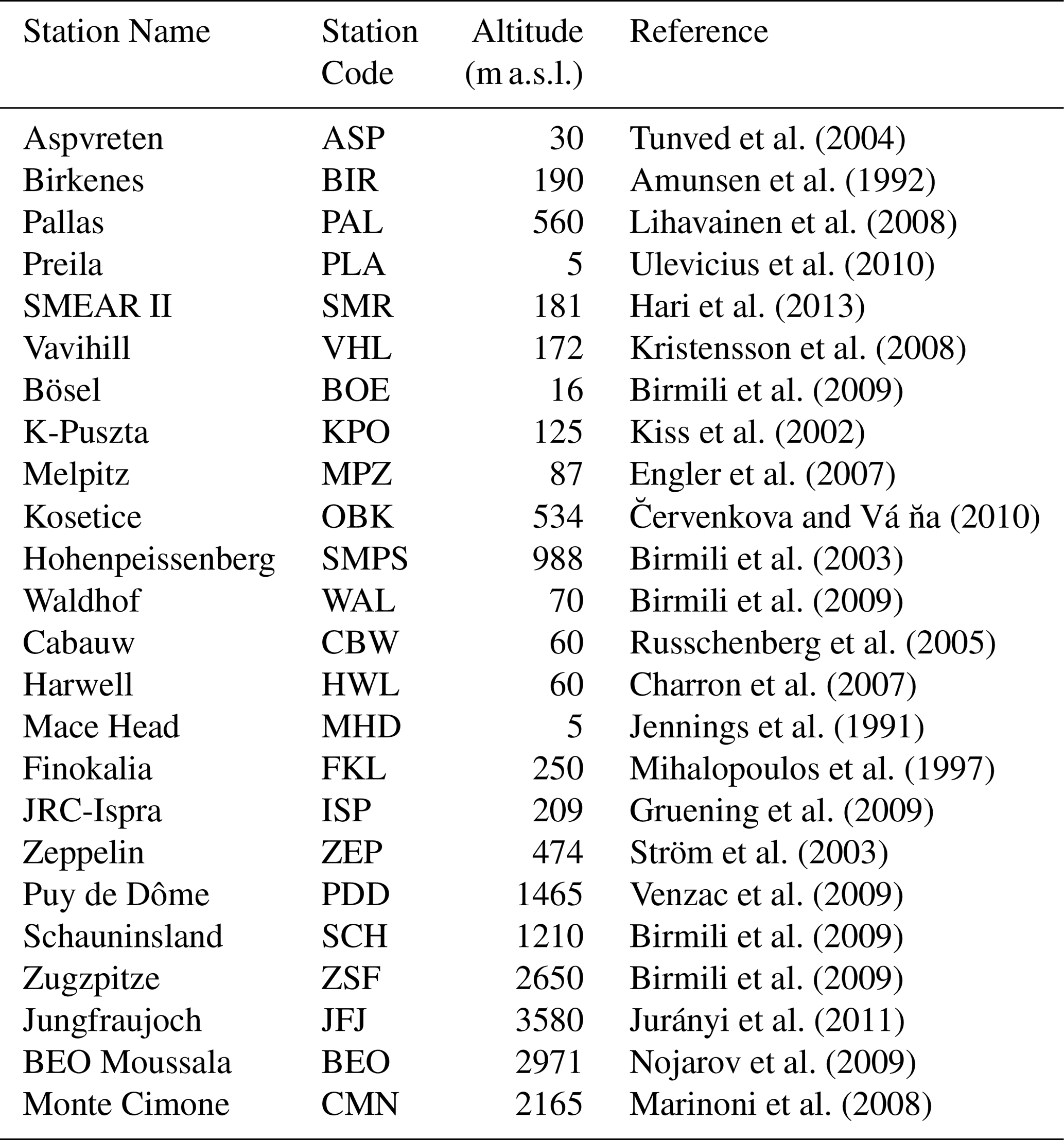
Besides synthetic data the neural network was evaluated on its ability to reproduce observations when driven by the MERRA-2 reanalysis output. This was important for testing the reliability of MAMnet when applied outside of the purely simulated environment. Near-surface aerosol number concentrations ranging from 30 to 500 nm, compiled by Asmi et al. (2011), were used for model evaluation. The dataset includes two years (2008–2009) of hourly measurements from 24 sites across Western Europe, as detailed in Table 3. These measurements were collected from two major monitoring networks: the European Supersites for Atmospheric Aerosol Research (EUSAAR) project, part of the Sixth Framework Programme of the European Commission (Philippin et al., 2009), and the German Ultrafine Aerosol Network (GUAN) (Birmili et al., 2009). The data are reported as cumulative number concentrations for four aerosol size ranges, N₃₀, N₅₀, N₁₀₀, and N₂₅₀, defined as,

$$\begin{array}{}\text{(2)}& N_X=\sum _{D_p=X}^{Y}N\left(D_p\right)\end{array}$$

where D_p is the aerosol dry diameter, and subscript X represents the aerosol number concentration for size range defined by threshold X, and Y=500 nm for $X=\mathrm{50},\mathrm{100}$ and 250 nm and Y=50 nm for X=30 nm. Equivalently, these can be calculated from the predicted ASD in the form (Seinfeld and Pandis, 2016),

$$\begin{array}{}\text{(3)}& \begin{array}{rl}{N}_X& =\sum _{i=\mathrm{1}}^{N_{\mathrm{mod}}}{\displaystyle \frac{N_i}{\mathrm{2}}}\left[\mathrm{erf}\left({\displaystyle \frac{\ln Y-\ln D_{\mathrm{pg},i}}{\sqrt{\mathrm{2}}\ln {\mathit{\sigma }}_{\mathrm{g},i}}}\right)\right.\\ & \left.-\mathrm{erf}\left({\displaystyle \frac{\ln X-\ln D_{\mathrm{pg},i}}{\sqrt{\mathrm{2}}\ln {\mathit{\sigma }}_{\mathrm{g},i}}}\right)\right]\end{array}\end{array}$$

where N_mod=7, is the number of lognormal modes. For each site, MERRA-2 derived aerosol mass concentration, temperature and air density are interpolated at the location and time of the measurements, then used in MAMnet to predict the ASD. Using Eqs. (1) and (3), N_X is predicted as the average of the two lowermost model levels (i.e., nearest the surface) and compared against the observations.

Tunved et al. (2004)Amunsen et al. (1992)Lihavainen et al. (2008)Ulevicius et al. (2010)Hari et al. (2013)Kristensson et al. (2008)Birmili et al. (2009)Kiss et al. (2002)Engler et al. (2007)C̆ervenkova and Vá n̆a (2010)Birmili et al. (2003)Birmili et al. (2009)Russchenberg et al. (2005)Charron et al. (2007)Jennings et al. (1991)Mihalopoulos et al. (1997)Gruening et al. (2009)Ström et al. (2003)Venzac et al. (2009)Birmili et al. (2009)Birmili et al. (2009)Jurányi et al. (2011)Nojarov et al. (2009)Marinoni et al. (2008)

Table 3 Datasets for the period 2008–2009 used for comparison with surface aerosol size distributions predicted by MAMnet. The original data reference is given, although all data sets used in this work were curated by Asmi et al. (2011).

We also used estimates of the concentration of cloud condensation nuclei, N_CCN to place MAMnet in the context of observationally-constrained estimates. To calculate N_CCN from MAMnet we folllowed the method of Fountoukis and Nenes (2005) to estimate N_CCN from the derived 7-modal size distribution and modal composition and the MERRA-2 fields as inputs. Hygroscopicity parameters, (κ) for each mode were obtained by volume-weighting the values for each aerosol species as listed in Table 1. Because N_CCN is strongly influenced by the ASD and composition, it serves as a useful diagnostic for evaluating the estimation of particle size. CCN concentrations are highly sensitive to aerosol size (Lee et al., 2013), as larger and more hygroscopic particles are more likely to activate into cloud droplets. As a result, N_CCN tends to be enhanced in populations dominated by such particles. Underestimation of particle size therefore translates into a lower N_CCN.

Global N_CCN datasets are typically derived from bulk aerosol mass using simplified assumptions about the ASD. For example, Choudhury and Tesche (2022) estimated N_CCN from spaceborne CALIOP (Cloud-Aerosol Lidar with Orthogonal Polarization) lidar measurements using pre-computed conversion factors. Block et al. (2024) derived N_CCN based on the latest Copernicus Atmosphere Monitoring Service (CAMS) reanalysis provided by the European Centre for Medium-Range Weather Forecast (ECMWF) by introducing assumptions on ASD and composition (Block, 2023). Similarly, The GiOcean atmosphere–ocean–aerosol reanalysis (Song et al., 2025), derived from the NASA GEOS-S2S system (Molod et al., 2020), incorporates a more advanced model framework. Unlike MERRA-2, which only assimilates the atmospheric state, GiOcean is a coupled atmosphere–ocean reanalysis that includes two-moment cloud microphysics, enabling the explicit calculation of N_CCN. Although GiOcean still relies on assumptions about aerosol size and composition, its CCN fields directly influence cloud processes and, in turn, aerosol evolution. In addition to comparing with reanalysis-based products, we evaluated MAMnet’s CCN predictions against in situ measurements from the Global Aerosol Synthesis and Science Project (GASSP) (Watson-Parris et al., 2019; Reddington et al., 2017). The GASSP dataset compiles aerosol and CCN measurements from 37 field campaigns and over 1000 aircraft flights, primarily concentrated over North America and Western Europe.

3 Results and Discussion

We evaluated the MAMnet model for both its ability to reproduce the GEOS+MAM7 model when driven by the testing data set, and to reproduce observations when driven by aerosol concentrations derived from the MERRA-2 reanalysis. We assessed whether MAMnet reproduces the spatial distribution of aerosol variables in GEOS+MAM7 using the the mean Pearson's spatial correlation coefficient (R). We also calculated the mean log-bias, i.e.,

$$\begin{array}{}\text{(4)}& \mathrm{MLB}={\displaystyle \frac{{\sum }_{n=\mathrm{1}}^{N_{\mathrm{samples}}}{\log }_{\mathrm{10}}\left(\widehat{\mathbf{Y}}\right)-{\log }_{\mathrm{10}}\left(\mathbf{Y}\right)}{N_{\mathrm{samples}}}},\end{array}$$

where $\widehat{\mathbf{Y}}$ and Y correspond to the predicted variables by MAMnet and GEOS+MAM7, respectively. In general MLB in the range $[-\mathrm{0.5},\mathrm{0},\mathrm{5}]$ indicates a prediction within an order of magnitude window around the target value. These metrics are summarized in Fig. 3 for each pressure level and output variable.

3.1 Evaluation against GEOS+MAM7

We first tested whether MAMnet had learned the physical relationships underlying the ASD or simply memorized the training data, and whether the model is able to conserve mass. To investigate this, we run MAMnet using MERRA-2 inputs, then recover the total mass of each species by mapping from the seven modes produced by MAMnet, as depicted in Fig. 1. Since aerosol concentrations in GEOS+MAM7 are not assimilated, they are expected to differ from MERRA-2, which incorporates observational constraints. If MAMnet had merely memorized the GEOS+MAM7 outputs, these same biases would persist when MERRA-2 inputs were used. Such a discrepancy would also indicate that MAMnet does not conserve mass as the total mass of each species would differ from the inputs.

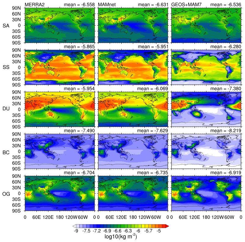
Figure 2 Comparison of column-integrated bulk aerosol. From top: sulfates plus ammonium (SA), sea salt (SS), dust (DU), black carbon (BC), and primary plus secondary organic matter (OG). Left panels correspond to MERRA-2, middle panels to the trained MAMnet model applied to MERRA-2 inputs, and right panels to the reserved GEOS+MAM7 test data.

Figure 2 compares the total aerosol mass column from MERRA-2 (left), MAMnet driven by MERRA-2 inputs (center), and GEOS+MAM (right). It is evident that GEOS+MAM7 tends to underestimate black carbon (BC) and sea salt (SS) over the ocean compared to MERRA2. If MAMnet had merely memorized the GEOS+MAM7 outputs, these same biases would persist when MERRA-2 inputs were used. Instead, MAMnet accurately reproduces the MERRA-2 aerosol concentrations when driven by MERRA-2 inputs, highlighting the internal consistency of the model as MAMnet is able to generalize to new, unseen data. This test also demonstrates that mass is conserved, as the total mass of each aerosol species is recovered showing very little bias.

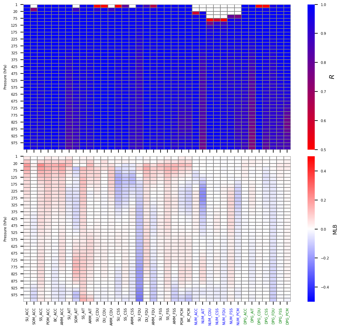
Figure 3 Pearson's spatial correlation (R) (top) and mean log-bias (Eq. 4; bottom) predicted by MAMnet calculated on the reserved test set, against the GEOS+MAM7 simulation. Results are shown for mass (Tables 1 and 2) and number (NUM) concentration for each mode, as well as for the derived modal diameter (DPG). Label color on the horizontal axis is added for emphasis.

Figure 3 summarizes the performance of MAMnet compared to GEOS+MAM7 across all output number and mass variables, as well modal size, for all model levels. MAMnet is able to reproduce the modal number concentrations (“NUM” variables in Fig. 3) from the GEOS+MAM7 simulations, with high spatial correlations R>0.9 and mean log-bias (MLB) within ±0.1 across most pressure levels. However, performance slightly degrades at pressures below p<100 hPa, particularly for the Aitken (NUM_AIT) and coarse dust modes (NUM_CDU), where correlations drop slightly (R>0.7) and MLB increases to ±0.3. The largest discrepancies occur near the surface (p>900 hPa) and in the upper troposphere (150–400 hPa). Specifically, NUM_AIT shows underprediction between 150–400 hPa while it overpredicts from 700–850 hPa, indicating that MAMnet tends to underestimate fine particles near the tropopause and overestimate them in the mid-to-lower troposphere. Similarly, NUM_PCM exhibits negative biases near 150–400 hPa, suggesting underprediction of particle number in the primary carbon mode at higher altitudes. The MLB patterns (Fig. 3, bottom panel) reveal localized biases at specific pressure ranges. Positive MLBs (orange shading) occur in NUM_PCM and NUM_ACC, indicating slight overestimation at mid-to-lower pressure levels. In contrast, NUM_CDU displays small negative MLB (blue shading) around 500–700 hPa, suggesting underprediction of coarse dust particles in the mid-troposphere. In summary, MAMnet captures overall modal number patterns well, but errors remain in the Aitken mode, primary carbon and coarse dust.

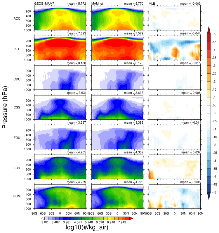
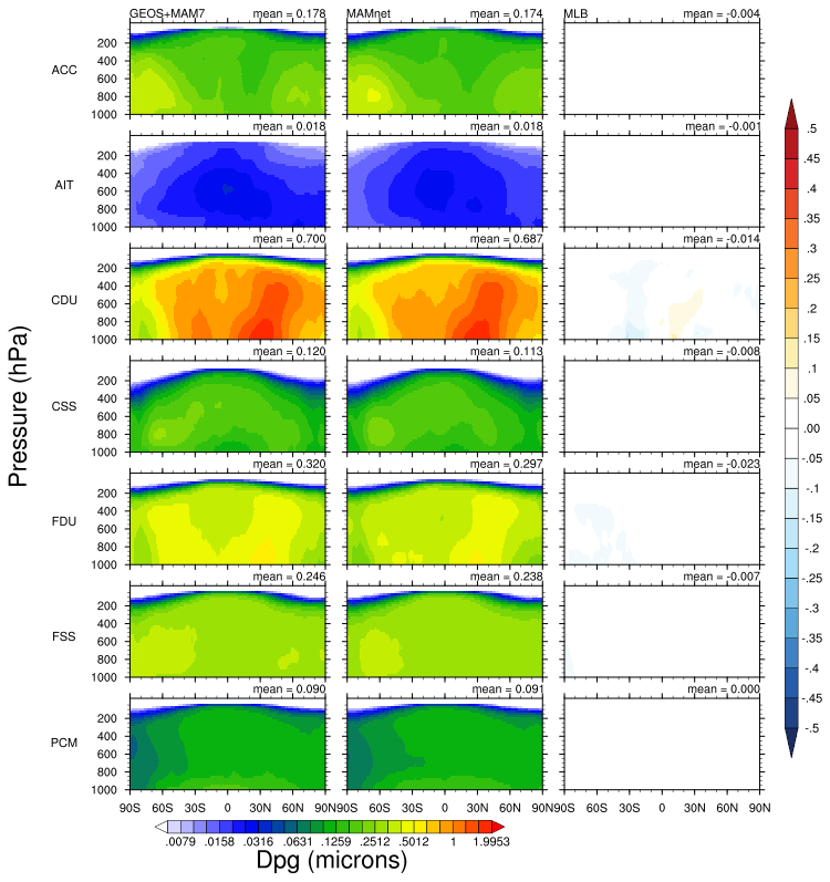
Figure 4 Zonal profiles for modal aerosol number concentration. Left: GEOS+MAM7 reserved test set. Middle: MAMnet prediction. Right: Mean Log-Bias. From top: Accumulation (ACC), Aitken (AIT), coarse dust (CDU), coarse sea salt (CSS), fine dust (FDU), fine sea salt (FSS), primary carbon matter (PCM).

Figure 4 shows the zonal mean profiles of modal aerosol number concentration, comparing GEOS+MAM7 outputs (left column), MAMnet predictions (center column). Consistent with Fig. 3, the Aitken mode exhibits the largest biases, characterized by underestimation above 400 hPa and overestimation in the lower troposphere, mostly below 700 hPa. Unlike other aerosol modes, the vertical distribution of Aitken mode particles is unique, with higher concentrations found in the upper troposphere and lower stratosphere (p<400 hPa) compared to lower altitudes, where the other modes exhibit the highest concentrations near the surface. The underestimation in the upper troposphere and overestimation in the lower troposphere may be influenced by a “dilution” effect, as Aitken particles contribute relatively little mass compared to other modes. This may be exacerbated in regions with active particle nucleation processes and combustion emissions which tend to disproportionately enhance number over mass concentration.

The accumulation mode (ACC), coarse sea salt (CSS), and fine sea salt (FSS) modes show generally strong agreement between true and predicted values, with minimal biases across most pressure levels, with MLB values close to zero. However, localized biases are apparent for FSS and PCM near the surface, suggesting slight overestimation in these regions. The coarse dust mode (CDU) and fine dust mode (FDU) exhibit minimal errors overall, with MLB values near zero across most pressure levels. MAMnet accurately predicts the aerosol number concentration for most modes, with systematic biases for the Aitken and primary carbon modes, particularly near the tropopause and in the lower troposphere, suggest that smaller particles are more difficult to predict accurately due to their unique vertical distribution and sparse representation in the data.

MAMnet accuately reproduces the spatial patterns of the aerosol mass, with accumulation mode mass variables such as SU_ACC, SS_ACC, and SOA_ACC showing high correlations (R>0.9) across the entire pressure range (Fig. 3). This is also the case for most other variables with only DU_FDU and AMM_FSS showing slight reduction in correlation near 1000 hPa, indicating slightly worse performance in the lower atmosphere. Biases shown in Fig. 3 (bottom) indicate that all but six mass tracers (SOA_ACC, SU_AIT, SOA_AIT, SU_CSS, SS_A_CSS, AMM_CSS) are systematically overpredicted for p<200 hPa where mass values are very small ($\sim {\mathrm{10}}^{-\mathrm{20}}$ kg kg⁻¹). These errors tend to be exacerbated in logarithmic space but remain negligible in absolute terms. Negative biases are also notable for SU_FDU and AMM_FDU, which become increasingly negative towards the surface. This is explained by the low mass of sulfate in the fine dust mode leading to a “dilution” of sulfate in fine dust mode relative to other aerosol modes. Overall, the model demonstrates robust predictive skill for most aerosol types, with minor discrepancies concentrated near the surface and in sparse aerosol regimes.

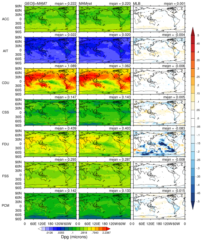
Figure 5 Modal geometric diameter, D_pg at 950 hPa. Left: GEOS+MAM7 reserved test set. Middle: MAMnet prediction. Right: Residual (log₁₀(MAMnet) − log₁₀(GEOS+MAM)). From top: Accumulation (ACC), Aitken (AIT), coarse dust (CDU), coarse sea salt (CSS), fine dust (FDU), fine sea salt (FSS), primary carbon matter (PCM).

Differences in the zonal distribution between aerosol modes can contribute to errors, especially due to the uneven representation of smaller particles, such as those in the Aitken and organic modes, in the training dataset, typically referred to as “class imbalance” (Japkowicz and Stephen, 2002; Buda et al., 2018). For instance, the mass of sulfate particles in the accumulation mode is often at least ten times greater than in the Aitken mode, whereas the opposite is true for the number concentration. As a result, the variability in sulfate mass is primarily driven by the accumulation mode, causing the Aitken mode to be underrepresented in the neural network's input data. Despite this, the residual differences between predicted and true values for Aitken mode aerosol number concentrations are small compared to other modes, and the mean global error remains well below an order of magnitude, highlighting the neural network's accuracy.

Figures 5 and 6 show the MAMnet-derived D_pg in agreement with GEOS+MAM7. It must be noted that D_pg is buffered against variation in mass and number concentration (Eq. 1). This buffering effect holds only if mass and number vary coherently. In practice, MAMnet predicts number concentration as a single output per mode, while mass is distributed across multiple species per mode. Unlike in the physical model, where mass and number are dynamically linked through the governing equations, MAMnet treats them as independent outputs. Therefore, accurate reproduction of D_pg by MAMnet is not guaranteed and must be learned implicitly. MLB for D_pg when tested against the test set is typically below 0.01, consistent with the high correlation coefficients for DPG (R>0.9), shown in Fig. 3. The fact that MAMnet is able to maintain low bias in D_pg without being explicitly constrained to do so suggests that the network has successfully learned a physically consistent relationship between mass and number.

The global distribution of D_pg for the different aerosol modes closely matches the spatial patterns of the modal number concentrations. Larger residuals are observed near the surface in the tropics and the Southern Hemisphere, particularly for fine dust (FDU). This discrepancy arises primarily due to the very low number concentrations of fine dust over the oceans, making it challenging for the neural network to accurately predict values close to zero. Residuals for D_pg in the coarse dust (CDU) mode are also slightly larger compared to other modes. This is evident in the zonal mean profiles (Fig. 6), where biases are most prominent in the tropics and near the Arctic. Additionally, MAMnet tends to underestimate D_pg in the Southern Hemisphere around 30° S, particularly in the free troposphere for fine dust. This underestimation likely results from class imbalance, as dust concentrations in this region are very low, making it difficult for the neural network to learn accurate predictions. It is also possible that MAMnet has learned associations biased toward aerosol-rich environments, which are more prevalent in the Northern Hemisphere.

Figure 6 As in Fig. 4, but for geometric mean diameter (D_pg) per mode.

3.2 Explainable machine learning analysis

Shapley values (Winter, 2002), originally developed in cooperative game theory, are now widely used to interpret predictions from neural networks (Kwon et al., 2023; Jeggle et al., 2023; Jia et al., 2024; Ma and Stinis, 2020; Lundberg and Lee, 2017). A Shapley value quantifies the contribution of a single input feature to a specific model prediction by comparing the prediction for a given sample to the average prediction across all samples. This contribution is averaged over all possible combinations of the remaining input features, referred to as coalitions. Because the number of such combinations grows rapidly with the number of features, we approximate Shapley values using 1000 randomly selected coalitions per calculation, facilitated by the SHAP python library using the kernel explainer method (Lundberg et al., 2020). In this study, Shapley values are used to assess the influence of each input feature on the predicted aerosol number concentrations for each mode.

Figure 7 shows a summary plot of Shapley values calculated for each input feature relative to predicted targets for aerosol modal number concentration (left) and mass (right). Each row represents a specific feature. The x-axis represents SHAP values, indicating the impact (positive or negative) of each feature on the model's prediction, so that the features with larger SHAP values contribute more significantly to the model output. Red dots represent high feature values, while blue dots indicate low feature values.

Features such as sulfate (SU), sea salt (SS), dust (DU), temperature (T), and air density (AIRD) are consistently ranked as dominant contributors, with their relative importance varying across aerosol modes. Fine-mode outputs, such as ACC and AIT, are strongly influenced by sulfate and temperature, where higher feature values positively impact predictions. In contrast, coarse-mode outputs like CDU and FDU are heavily driven by dust, with significant positive contributions observed for high dust concentrations. Intuitively, this makes sense as SU, SS, and DU are the largest components of accumulation mode aerosols. However the relation is non-linear as high SU values correspond to a strong positive impact on aerosol number, particularly for dust (CDU) and sea salt (CSS) modes, whereas low values lead to neutral or negative contributions.The SHAP values further highlight the critical role of air density and temperature in for CSS and FSS, which may be related to the aerosol activation processes.

For aerosol mass, the SHAP plots show significant influence from DU, SS, BC, SU. The interplay between feature importance and values is evident as, high sea salt concentrations (SS) are positively correlated with increased mass in CSS, while low values lead to neutral or negative contributions. One significant characteristic of the mass SHAP plots is the broader range of SHAP values compared to number concentration, indicating greater variability in the importance of input features for predicting mass. For instance, black carbon (BC) has a consistently positive influence on ACC and AIT mass predictions, but its impact is less pronounced for other modes. Additionally, temperature at low values negatively impacts aerosol mass, while at higher values, it positively influences mass. In some cases however a SHAP value for a feature may have no obviously interpretable significance to the target prediction, or may be so strongly correlated with another feature that the individual contribution is negligible with respect to the feedbacks between a pair of features or more (Aas et al., 2021).

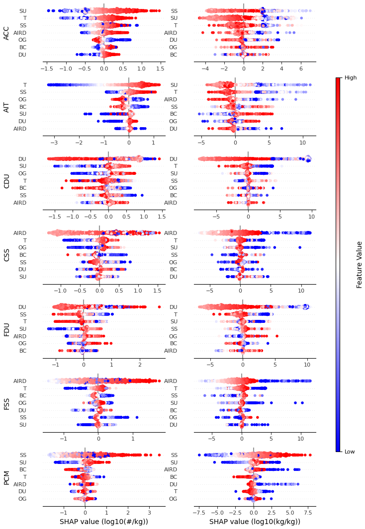
Figure 7 SHAP analysis for aerosol number concentration (left) and total mass (right) across different modes in the troposphere, based on 1000 randomly selected samples from the test set. Modes are displayed from top to bottom: Accumulation (ACC), Aitken (AIT), coarse dust (CDU), coarse sea salt (CSS), fine dust (FDU), fine sea salt (FSS), and primary carbon matter (PCM). The color gradient (red for high values, blue for low values) indicates the relative value of each feature, with features ordered top-to-bottom by their importance to the prediction (most sensitive at the top). The x-axis represents SHAP values, quantifying how much each feature contributes to deviations from the mean prediction.

3.3 Evaluation against observations

The ability of a neural network to generalize to new data is a key measure of its effectiveness and reliability in real-world applications. While the neural network may perform well reproducing simulated data, it is important to test whether MAMnet is able to reproduce patterns observed in nature. To accomplish this, we take advantage of the ability of MAMnet to work with reanalysis data, that is, using as input the assimilated fields of MERRA-2.

MERRA-2 includes aerosol mass fields that are constrained by satellite observations through data assimilation (Buchard et al., 2017; Sun et al., 2019; Ukhov et al., 2020; Gueymard and Yang, 2020; Su et al., 2023), and thus provides a more realistic input compared to free-running model simulations. Although GEOS+MAM7, which was used to train MAMnet, does not assimilate aerosols and cannot be directly compared to observations at specific sites, it provides physically consistent mass and number concentrations from which the network learns the relationship between these quantities. When applied to MERRA-2, MAMnet combines this learned relationship with more observation-constrained aerosol mass fields, allowing us to evaluate how well it maintains physical consistency in a more realistic setting. This comparison does not validate MAMnet independently of its training data but serves to assess its performance when driven by the best available mass estimates.

3.3.1 Comparison against ground observations

Figure 8 compares the cumulative ASD predicted by MAMnet against surface observations from different European sites. These are mostly coastal sites with composition typical of clean and polluted continental origin, that is, mostly of sulfates, dust, organics and sea salt (Asmi et al., 2011). Altitude ranges from a few meters to about 3 km providing a good overview of the lower troposphere. Although representing a limited set, the range of aerosol compositions, sources, and altitudes offers a meaningful assessment of the model's ability to generalize to different atmospheric states. To carry out the comparison, MAMnet was run using collocated aerosol concentrations and meteorological fields obtained from MERRA-2 at each site, and using Eq. (3). MAMnet results represent the average of the two lowermost model layers (roughly 200 m above the surface).

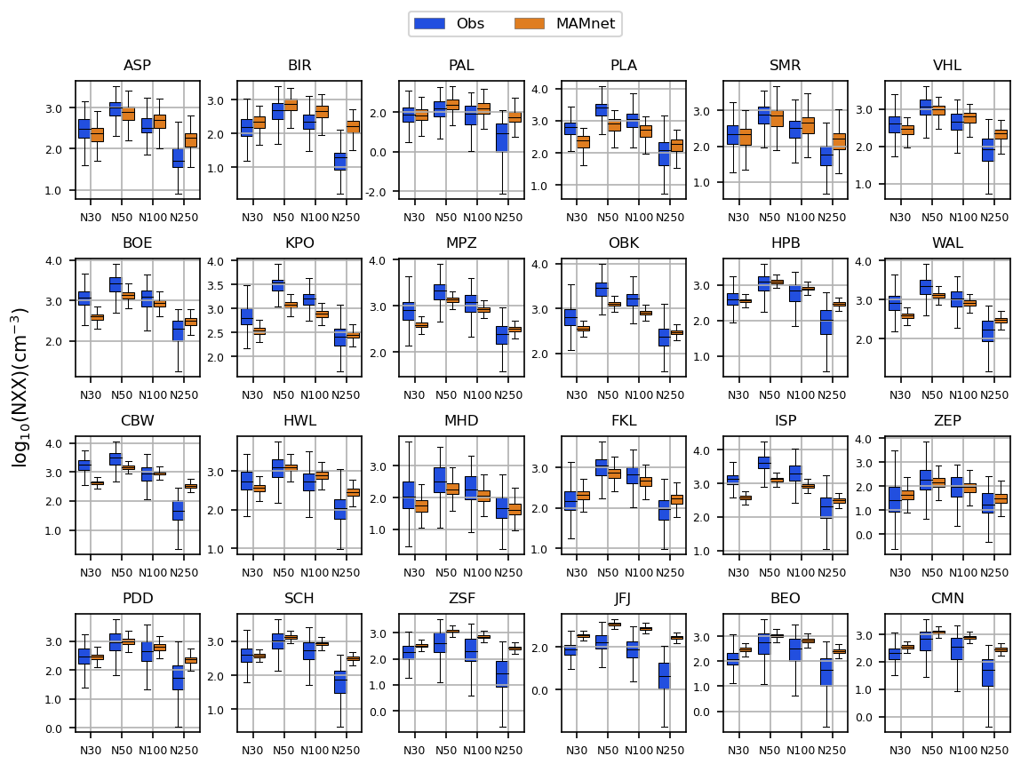
Figure 8 Cumulative size distribution comparison of the trained MAMnet model applied to MERRA-2 inputs against surface measurements (Asmi et al., 2011). The sites in the bottom row (PDD, SCH, ZSF, JFJ, BEO, CMN) are characterized as high altitude sites, with altitudes between 1200 and 3600 m a.s.l.

Except for high altitude sites (Fig. 8, bottom row), MAMnet tends to predict slightly lower median values compared to observations, with this discrepancy becoming more pronounced as particle size increases (N100 and N250). This is particularly noticeable at locations such as PAL, PLA, OBK, MHD, FKL, and JFJ, where the model underestimates values consistently. The pattern is reversed at high-altitude sites (PDD, SCH, ZSF, JFJ, BEO, and CMN), where median N100 and N250 are generally overestimated by MAMnet, although the observations themselves display significant variability. Some locations like SMR, WAL, CBW, and SCH exhibit better agreement, with overlapping medians and interquartile ranges. Additionally, the spread of values for MAMnet is typically narrower than for observations, indicating that the model underestimates variability. Observations also show more outliers, whereas MAMnet predictions are more constrained. There are a few exceptions where MAMnet slightly overestimates values, such as VHL (N250) and SMR (N100). Overall, systematic bias exists in MAMnet-predicted particle concentrations, particularly for larger size bins, capturing less variability compared to observations.

Errors in the estimated ASD may originate from the training data (GEOS+MAM7) or from the MERRA-2 fields used as input to MAMnet. To assess the potential impact of the training data, we collocated the average ASD at each site using the GEOS+MAM7 test dataset. This analysis is intended to evaluate whether GEOS+MAM7 exhibits, on average, the same biases shown in Fig. 8, rather than assessing point-by-point predictions as done for MAMnet. Figure 9 shows that GEOS+MAM7 and MAMnet indeed display similar biases relative to the observations, suggesting that errors in the training data are partially inherited by MAMnet. However, a comparison of Figs. 8 and 9 also indicates that the use of MERRA-2 inputs tends to reduce variability in the ASD. For each size bin, the interquantile range is substantially narrower in the MAMnet results. This effect is particularly pronounced at high-altitude sites (bottom row in both figures).

MERRA-2 may not resolve local emissions, terrain, or small-scale meteorology, such as boundary layer height and humidity. This can lead to biases, particularly in the larger particle size categories that depend on aerosol growth processes. Moreover, despite representing better ASD variability, the training data lacks sufficient diversity, particularly for remote or high-altitude sites, which are also underrepresented in the training set. Additionally, aerosol evolution involve complex, nonlinear interactions that are not explicitly modeled by MAMnet. These factors likely contribute to the model's challenges in capturing the magnitude and variability of aerosol concentrations observed in the real world. Additionally, it is important to note that retrievals of ASD are inherently complex, and experimental errors can be significant, particularly for larger particle sizes (Asmi et al., 2011). Nevertheless, the consistent results across many sites indicate that MAMnet is capable of reasonably capturing the ASD on regional scales when driven by reanalysis data.

3.3.2 Comparison against global CCN datasets

Figure 10 illustrates the global mean distribution of cloud condensation nuclei (CCN) at 0.2 % supersaturation at 900 hPa, derived from MAMnet driven by MERRA-2 (shown as MAMnet-MERRA2), GiOcean (Song et al., 2025), the CAMS aerosol reanalysis (Block et al., 2024), and CALIOP satellite retrievals (Choudhury and Tesche, 2022). Data were averaged over the period 2006–2021. All datasets display on average lower CCN concentrations over oceans, particularly in polar regions, and higher concentrations over land particularly in central and eastern Asia, Europe, and the Americas. However, large differences in absolute values are evident with MAMnet-MERRA2 consistently showing the lowest N_CCN, and CALIOP-derived the highest. These discrepancies likely arise from differing assumptions in estimation methods. GiOcean and CAMS estimate CCN based on aerosol mass, prescribing the ASD, and assuming externally-mixed aerosols, which may double-count CCN as organics and sulfates are typically internally mixed (Adachi and Buseck, 2008; Kirpes et al., 2018). MAMnet-MERRA2 avoids this issue but underpredicts N_CCN over oceanic regions, likely due to low sea salt concentrations in MERRA-2, stemming from uncertainties in the aerosol assimilation system (Buchard et al., 2017). In contrast, CALIOP may overestimate N_CCN from the assumption of CCN as all soluble aerosols above 50 nm, some of which may not activate as CCN at 0.2 % supersaturation.

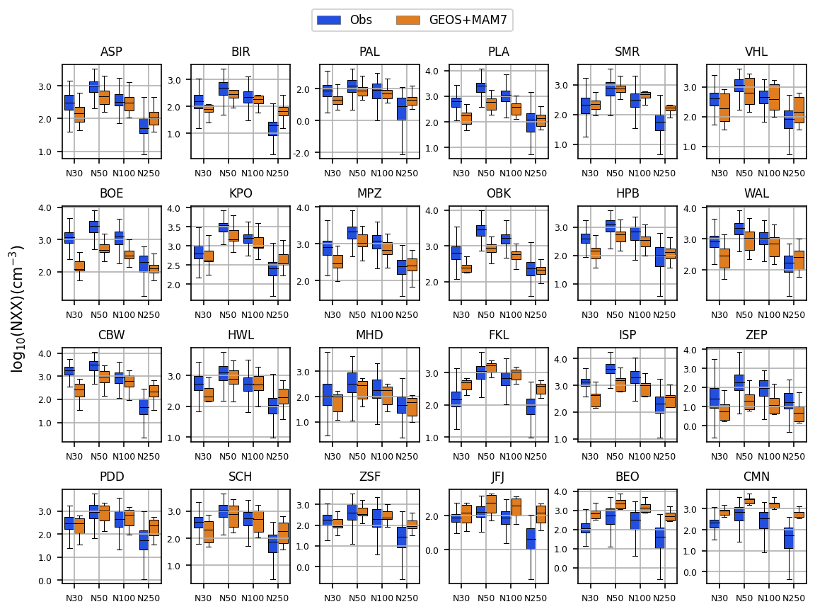
Figure 9 Average cumulative size distribution comparison of the GEOS+MAM7 test data against surface measurements (Asmi et al., 2011). The sites in the bottom row (PDD, SCH, ZSF, JFJ, BEO, CMN) are characterized as high altitude sites, with altitudes between 1200 and 3600 m a.s.l.

Figure 11 compares global mean vertical profiles of N_CCN from the datasets in Fig. 10 and from in-situ observations (Watson-Parris et al., 2019). Vertical distributions vary significantly. GiOcean, CALIOP, and in-situ profiles exhibit similar shapes with peak concentrations around 950 hPa, while the MAMnet-MERRA2 and CAMS profiles show a monotonic decrease with altitude. The peak in N_CCN at 950 hPa may result from more efficient aerosol scavenging near the surface, better represented by two-moment cloud microphysics in GiOcean (Song et al., 2025; Barahona et al., 2014). In contrast, MAMnet-MERRA2 and CAMS rely on single-moment cloud microphysics, which may explain the smoother decrease in N_CCN with height. The reliance on single-moment microphysics may also explain the more gradual decrease in N_CCN with height in CAMS and MAMnet-MERRA2 than in the other data sets, noticeable over the ocean. In the free troposphere, MAMnet-MERRA2 aligns more closely with GiOcean, CALIOP and the in situ data.

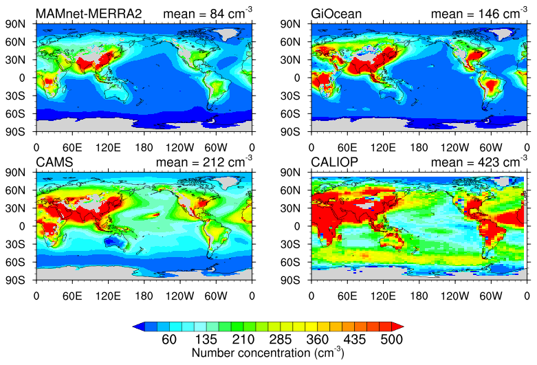
Figure 10 MAMnet-derived CCN at 0.2 % supersaturation at 900 hPa using the MERRA2 reanalysis (MAMnet-MERRA2) against global CCN datasets. Also shown are results from the GiOcean reanalysis (Song et al., 2025), CALIOP- (Choudhury and Tesche, 2022), and CAMS- (Block et al., 2024) derived CCN.

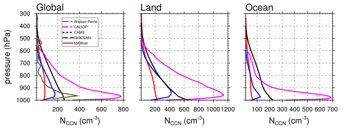
Figure 11 Annual mean profile of CCN concentration derived from MERRA2 using MAMnet (red). Also shown are CALIOP-derived CCN (magenta;  Choudhury and Tesche, 2022), the GiOcean reanalysis (blue;  Song et al., 2025), CCN derived from field campaign data around the globe (green;  Watson-Parris et al., 2019), and CAMS-derived CCN (black;  Block et al., 2024).

4 Conclusions

This study develops a neural network, termed MAMnet, to predict the aerosol size distribution and mixing state using as input the bulk mass of different aerosol species, temperature and density. MAMnet is oriented towards allowing a better estimation of the ASD and the aerosol physicochemical properties in cases where computational cost considerations prevent the usage two and higher moment aerosol microphysics schemes, for instance, weather forecast, or where limited information is available to constraint the ASD as in remote sensing and data assimilation. The neural network was optimized for performance taking into account the model architecture, training parameters and the rank of the data used as input.

MAMnet is designed to reproduce the mapping from aerosol mass to size distribution as generated by the MAM7 scheme within the GEOS system. As such, it inherits the assumptions and meteorological context of the training simulations. However through a comprehensive evaluation of the NN model against simulated data and observations, we demosntrated that MAMnet is a robust and accurate model over a wide set of conditions. Importantly, MAMnet reproduces MERRA-2 aerosol concentrations when driven by MERRA-2 inputs, demonstrating that it has learned physical relationships rather than memorizing the training data, conserving the total aerosol mass. Explainable machine learning analysis showed that MAMnet identifies key physical drivers and the non-linear behavior governing the aerosol distribution across fine and coarse scales.

Comparison of MAMnet predictions against a reference dataset from GEOS+MAM7 simulations resulted in good agreement, with log-mean residuals typically below 0.1 and spatial correlation typically exceeding 0.9 for all aerosol modes. The greatest discrepancies were observed near the surface and in regions with low aerosol concentrations i.e., fine dust over oceans and coarse dust in the Southern Hemisphere free troposphere. These discrepancies are primarily attributed to challenges in the prediction of concentrations near zero and class imbalance. Notably, biases in number and mass concentrations do not significantly influence the prediction of geometric mean diameter, indicating that MAMnet captures the physical consistency between aerosol mass and number, inherently conserving mass.

We took advantage of the fact that MAMnet can be driven by output from reanalysis data to evaluate its performance against observations. When driven using collocated MERRA-2 fields, MAMnet reasonably reproduced the measured aerosol size distribution at different ground observation sites, representing a variety of aerosol composition, origin and meteorological conditions. The median values of the predicted number concentrations were generally consistent with observations. However the range of values predicted by MAMnet is in general smaller than observed, indicating that the model underestimates variability. It is likely that coarse reanalysis inputs, limited training data diversity, and the complexities of aerosol evolution, not modeled explicitly by MAMnet, contributed to the observed discrepancies.

CCN concentrations derived from MAMnet using the MERRA2 dataset were within the range of reported values but showed discrepancy near the surface and in regions with high variability, which may originate from uncertainty in the MERRA-2 aerosol fields. As MAMnet reproduces well the training dataset it is likely that the biases against observations result from biases in the input and complex physics not modelled by MAM7. At this point it is difficult to explicitly attribute sources of error in MAMnet and this is left for future research. Despite such biases, the comparison against observations indicate that MAMnet is able to capture the aerosol size distribution on regional and global scales.

Strategies to address the remaining biases include applying physical constraints via transfer learning, as well as including observational data during the training process (Barahona et al., 2024). Class imbalance can potentially be addressed by reconfiguring the NN such that each mode would be predicted by a separate layer, or even individual NNs. The latter option is less desirable because it would require developing, constraining, and maintaining multiple NNs as opposed to one. Future work would focus on applying MAMnet to elucidate long-term trends in the ASD as well as on its implementation with GCMs (Ott et al., 2020). MAMnet is designed to be resolution-agnostic, but the relationship between aerosol mass and size distribution may vary with model resolution and it is suggested to be explored in future work. Including additional input variables, such as gaseous species or solar radiation, may make MAMnet predictions more physically interpretable. Neverthless, the model developed here provides a versatile foundation to improve the physical representation of aerosols in weather forecasting, remote sensing and data assimilation, potentially enhancing our understanding of their role in the climate system.

Appendix A: Network Training and Optimization

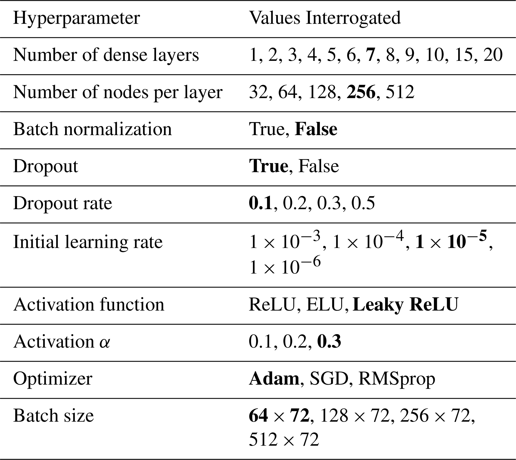
The MAMnet model was trained using the Keras library with Tensorflow backend (Chollet, 2015). Optimization was carried out with the Adam algorithm (Kingma and Ba, 2014) using the minimum mean square error (MSE) as the loss function, with no additional constraints. Hyperparameter optimization for MAMnet was performed using the Keras Tuner software (O'Malley et al., 2019). Approximately 1500 optimization trials were performed using random configurations of the hyperparameters in Table A1, using a subset of the training data as in Yu et al. (2024). All trials used the same subset of the training/validation data (5 output files for training, 2 for validation). For each parameter set, a new model was built and trained for up to 100 epochs with the same early stopping criteria used during the training of MAMnet. For each trial, a custom metric was recorded at the end of each epoch, the convergence loss (ℒ_conv), defined as the absolute difference between the training and validation losses. Using this custom metric allowed us to select the model that generalizes the best over both the training and validation data sets. The best set of hyperparameters was selected by choosing the configuration that minimized the MSE on the validation set and had the lowest ℒ_conv.

Table A1 Parameters used during hyperparameter tuning for MAMnet. Optimal hyperparameters are shown in bold.