The spatio-temporal visualization tool HMMLVis in renewable energy applications

Understanding causal relationships in multivariate time series is essential across many scientific domains, especially in climatology and meteorology where complex dependencies drive extreme events. Existing tools often lack intuitive visualization, particularly for heterogeneous Granger causality applied to non-Gaussian data such as time series following exponential distributions. There is a need for an accessible, interpretable tool that helps scientists explore temporal dependencies and uncover causal structure in such settings. We present HMMLVis, an original visualization tool designed for multivariate and heterogeneous Granger causal inference (Heterogeneous Granger causality by Minimum Message Length). The tool supports causal discovery in time series with exponential distributions and offers an intuitive interface for exploring temporal relationships. While HMMLVis is applicable across disciplines dealing with time-series data, this work focuses on its use in climatological and meteorological contexts. We demonstrate HMMLVis on several applications involving meteorological phenomena affecting the upper and lower distributional tails, using datasets from renewable energy (wind and PV), air pollution, and the European Meteorological Network (EUMETNET) post-processing benchmark (EUPPBench) across different temporal horizons. Our results show that HMMLVis successfully recovers known causal relationships and additionally reveals previously unobserved temporal dependencies relevant to the specific cases examined. As an interpretable and user-friendly visualization tool, HMMLVis has strong potential to support climatologists, meteorologists, and other researchers working with complex time-series data. By enabling clearer insight into causal interactions, it contributes to more informed scientific understanding and facilitates knowledge discovery across multiple environmental and atmospheric science applications.

1 Introduction

In large-scale complex dynamical systems such as meteorology/climatology and fields and system affected by meteorological and climatological conditions such as renewable energy production systems, replicated interventional experiments are rarely feasible or ethically problematic. The rapidly increasing amount of observations and numerical-dynamical generated data, e.g. reanalysis or numerical weather prediction data, opened the very fast developing field of data-driven deep learning forecasting methods. In data-driven predictions, the interplay of features and causality gain more importance in improving the forecast quality and skill. Applying observational causal discovery methods can help to improve predictions by their ability to quantify potential causal dependencies from time series data without the need to intervene in systems (e.g. manipulate part of a system and infer relationships from the consequences).

In contrast to deep learning, which mainly focus on prediction and classification, causal inference methods aim at discovering and quantifying the causal dependencies of the underlying system. Although interpreting deep learning models is an active area of explainable AI, extracting the causes of particular phenomena, e.g., extreme flooding, from a deep learning structure with multiple layers is usually not possible. Conversely, causal inference methods can contribute in theoretical understanding of the underlying system and, combined with deep learning methods, can help improving predictions and classifications. Recently more attention was brought to causal methods in climatology, as Runge et al. (2023) have introduced a taxonomy of research questions. These are types of expert assumptions and properties of the available time series data to provide a causal language in which researchers can define their study questions. To make these causal methods even more accessible, they could be provided in visual tools for researchers to perform experiments on observation data.

Our work presents a visual tool in HMMLVis, which uses a method extending Granger causality, named HMML, to infer causal relationships in time-series data. Granger causality addresses causal relationships quantitatively by comparing the prediction error of time-series models given the inclusion or exclusion of another variable's model.

In its original linear form as introduced in Granger (1969), criticism arose as Granger causality does not take counterfactuals into account (Mannino and Bressler, 2015; Maziarz, 2015) and does not fulfill the causal sufficiency, i.e. non-existence of a hidden common cause (Spirtes, 2010). Further, the regression equations reflect only correlations and the Granger test detects only “predictive causality”. In defense of the method, Granger (1988) wrote:

Possible causation is not considered for any arbitrarily selected group of variables, but only for variables for which the researcher has some prior belief that causation is, in some sense, likely.

In other words, drawing conclusions of the existing causal relation between a time series and its direction is only possible if some theoretical knowledge of mechanisms connecting the time series is accessible. Granger stressed that a proper use of Granger causality would require to condition on all relevant variables in the world. In fact, conditioning on the “whole universe” is a deficiency not only of the Granger causal model but of most models used for multivariate causal inference, including the structural causal models (SCM), e.g. Spirtes et al. (2000), since not always all variables (direct, confounding, latent) are known and using such a high degree of parameters would blow up every modeling system. This condition is, in practice, relaxed by an assumption that the set of all relevant variables is known. Thus, the selection of relevant variables is a necessity and extremely crucial step and cannot be done without domain experts. Therefore, here we assume a set of relevant parameters with the assumption of causal relationship between them provided by expert domain knowledge. Granger causal inference can also answer certain counterfactual questions when applied to observational data which can be pooled or data of seasonal nature, e.g. of climatological origin.

Thus it is generally accepted that Granger causality does not capture all aspects of causality but enough to be worth considering for empirical test (Singh and Borrok, 2019). In observational data, namely meteorological and climatological time series, where replicated interventional experiments are hardly feasible, Granger causality and its non-linear and graphical variations can provide a valuable insight into the the temporal relationships about variables. Thus, besides the rapid development of other causal inference methods, Granger causality and its non-linear and multivariate versions still play an important role in Earth system sciences, as demonstrated by the unremitting publications this field, e.g. on prediction in photovoltaic data set (Shan et al., 2023), environmental quality assessment (Celik and Alola, 2023), or in general renewable energy production (Dumrul et al., 2023). Urban air quality constitutes another relevant application domain in which causal discovery can provide added value. Pollution episodes such as winter inversions in Alpine basins are driven by a complex interplay between meteorology, e.g. wind stagnation, humidity, boundary-layer dynamics) and aerosol processes. Previous studies have used Granger-based methods to analyse the drivers of PM_2.5 (e.g. Zhu et al., 2015b; Alvarez-Castellanos et al., 2023a), yet visualization tools to interpret such causal structures remain limited. By integrating Copernicus Atmosphere Monitoring Service (CAMS) reanalysis aerosol and meteorological fields, HMMLVis allows users to explore these causal relationships in a transparent and temporally resolved manner.

In this work, we present our original visualization tool for Granger causal inference, HMMLVis, namely for the case of heterogeneous Granger causality (Behzadi et al., 2019). The tool is demonstrated on different types of applications related to meteorological events, namely renewable energy production by photovoltaic and EUMETNET postprocessing benchmark data set (EUPPBench) from Demaeyer et al. (2023). Further, other utilization of HMMLVis is discussed for air polution data, semi-synthetic wind production data for a selected wind farm location and for semi-synthetic photovoltaic power generation. In addition to energy-related applications, HMMLVis is demonstrated using an urban air quality (UAQ) case study. This example is included to illustrate how the tool can be used to explore heterogeneous causal relationships between meteorological drivers and air-pollution variables in realistic environmental time series, rather than to provide a comprehensive atmospheric chemistry assessment.

The paper is organized as follows. Section 2 presents heterogeneous Granger causality and Method HMML and Sect. 3 describes related work. Our HMMLVis method is introduced in Sect. 4. Workflow and description of the visualization tool of HMMLVis is explained in Sect. 5. Section 6 discusses utilization of HMMLVis in several climatological or energy-production applications as well as runtime of the HMMLVis tool. Our conclusions are summarized in Sect. 7.

2 Heterogeneous Granger Causality and Method HMML

The original bivariate concept of causality defined by Granger (1969) can be extended to the multivariate case, i.e. for p>2 time series and a time lag d≥1, indicating the maximum number of lagged observations included in the model, the so-called model order. This model order can be selected via an information theoretic criteria such as the Bayesian or Akaike information criterion. For p time-series ${\mathit{x}}_{\mathrm{1}},\mathrm{\dots },{\mathit{x}}_p$ the vector auto-regressive (VAR) model is:

$$\begin{array}{}\text{(1)}& x_i^t={\mathit{X}}_{t,d}^{\mathrm{Lag}}{\mathit{\beta }}_i^{\prime }+{\mathit{ϵ}}_i^t\end{array}$$

where ${\mathit{X}}_{t,d}^{\mathrm{Lag}}=(x_{\mathrm{1}}^{t-d},\mathrm{\dots },x_{\mathrm{1}}^{t-\mathrm{1}},\mathrm{\dots },x_p^{t-d},\mathrm{\dots },x_p^{t-\mathrm{1}})$, ${\mathit{\beta }}_i^{\prime }$ is the transposition of the matrix β_i of the regression coefficients and ϵ^t the error (Behzadi et al., 2019). It is stated that the time-series x_j Granger-causes the time-series x_i for lag d if and only if at least one of the d coefficients in row j of β_i is non-zero. Thus, to detect causal relations, coefficients of the VAR model need to be estimated. This problem can be solved by a penalization approach of the order d, e.g. by using Lasso (Tibshirani, 1996), often also referred to as variable selection method.

Multivariate Granger causality among time series from Eq. (1), as an instance of graphical causal models (Glymour et al., 2019), assumes that random error time series follow Gaussian distributions with zero mean and constant deviation. In many applications however, these assumptions do not hold and using a graphical Granger model can lead to an inaccurate causal inference results. Profiting from the framework of the generalized linear models (GLM) introduced in Nelder and Wedderburn (1972) and Behzadi et al. (2019) proposed a general model to detect Granger-causal relations among p≥3 number of time series which follow a distribution from the exponential family (where Gaussian distribution is a special case). The relation among the response variable and the covariates in a regression is not linear anymore but defined by a so-called link function η, a monotone twice differentiable function depending on the concrete distribution functions from the exponential family. The best-fitting distribution of the target time series within each interval can be identified using the Residual Sum of Squares (RSS) and the Kolmogorov–Smirnov (K–S) test.

The heterogeneous graphical Granger model (HGGM, Behzadi et al., 2019), considers time series x_i which follow a distribution from the exponential family using a canonical parameter θ_i. The HGGM uses the idea of generalized linear models and applies them to time series in the following form

$$\begin{array}{}\text{(2)}& x_i^t\approx {\mathit{\mu }}_i^t={\mathit{\eta }}_i^t\left({\mathit{X}}_{t,d}^{\mathrm{Lag}}{\mathit{\beta }}_i^{\prime }\right)={\mathit{\eta }}_i^t\left(\sum _{j=\mathrm{1}}^p\sum _{l=\mathrm{1}}^d{x}_j^{t-l}{\mathit{\beta }}_j^l\right)\end{array}$$

for $x_i^t$, $i=\mathrm{1},\mathrm{\dots },p,t=d+\mathrm{1},\mathrm{\dots },n$ each having a probability density from the exponential family; μ_i denotes the mean of x_i and $\mathrm{var}\left({\mathit{x}}_i\right|{\mathit{\mu }}_i,{\mathit{\varphi }}_i)={\mathit{\varphi }}_i{v}_i({\mathit{\mu }}_i)$ where ϕ_i is a dispersion parameter and v_i is a variance function dependent only on μ_i; ${\mathit{\eta }}_i^t$ is the tth coordinate of η_i. The causal inference in Eq. (2) can be solved as a maximum likelihood estimate for β_i for a given lag d>0, λ>0, and all $t=d+\mathrm{1},\mathrm{\dots },n$ with added adaptive lasso penalty function (Behzadi et al., 2019). One can state that time series x_j Granger–causes time series x_i for a given lag d, and denote x_j→x_i, for $i,j=\mathrm{1},\mathrm{\dots },p$ if and only if at least one of the d coefficients in j−th row of $\widehat{{\mathit{\beta }}_i}$ of the penalized solution is non-zero, see Behzadi et al. (2019).

The concept explained in this paragraph replaces the solution via p penalized linear regression problems by formulating the feature selection as a combinatorial optimization problem, as it was done in Hlaváčková-Schindler and Plant (2020a) for the multivariate Granger causal model with Gaussian time series and in Hlaváčková-Schindler and Plant (2020b) for the multivariate Granger causal model with time series from the exponential family. The second method uses the information theoretic criterion “minimum message length” (MML), introduced by Wallace (2005) for general inference problems, to determine causal connections in the model, improving the results especially for short time-series. This will be the focus of the following work, as e.g. in the wind related data set, we initially analyze measurements of 96 samples.

The MML principle is a formal information theory restatement of Occam’s razor: Even when models have a comparable goodness-of-fit to the observed data, the one generating the shortest overall message is more likely to be correct (where the message consists of a statement of the model, followed by a statement of data encoded concisely using that model). The statistical version of the MML principle constructs a description in terms of probability functions and some prior knowledge of the parameter vector. MML seeks the model that minimizes this trade-off between model complexity and model capability. In the type of MML considered in Hlaváčková-Schindler and Plant (2020b) and in this study and application, the parameter space θ for the statistical model $p(.|\mathit{\theta })$ is decomposed into a countable number of subsets and associated code words for members of these subsets. The parameter θ in the MML criterion corresponds to the maximum likelihood estimates of the regression coefficients and the dispersion coefficient of the target time series. The regression problem is expressed for $i=\mathrm{1},\mathrm{\dots },p$ via incorporation of a subset of indices of regressor variables, denoted by ${\mathit{\gamma }}_i\subset \mathit{\{}\mathrm{1},\mathrm{\dots },p\mathit{\}}$ and $k_i=\left|{\mathit{\gamma }}_i\right|$ into Eq. (2)

$$\begin{array}{}\text{(3)}& x_i^t={\mathit{\eta }}_i^t\left({\mathit{X}}_{t,d}^{\mathrm{Lag}}\left({\mathit{\gamma }}_i\right){\mathit{\beta }}_i^{\prime }\right)={\mathit{\eta }}_i^t\left(\sum _{j=\mathrm{1}}^k\sum _{l=\mathrm{1}}^d{x}_j^{t-l}{\mathit{\beta }}_j^l\right).\end{array}$$

The best structure of γ_i in the sense of MML principle is determined either by a genetic or exhaustive search algorithm, for more details see Hlaváčková-Schindler and Plant (2020b).

Remarks. The value of time lag (i.e. the model order) of the target variable in HMML can be determined by expert knowledge or by the information theoretic criteria, similarly as for the problem (1). Since HMML is an instance of GLM models, the consequences about collinear or almost collinear time series hold also for HMML. Collinearity does not violate any assumptions of GLMs, unless there is perfect collinearity.

2.1 Limitations of Classical Granger Models and Advantages of HMML

Method HMML in general has the following advantages. It supports mixed data: HMML can work with both continuous and discrete variables, which is a major advantage over classical Granger causality methods that typically assume all variables are continuous and Gaussian. HMML handles nonlinear and non-Gaussian data. Further, it allows for modeling interactions between variables of different types without needing to transform or homogenize the data. The MML criterion balances model complexity and goodness of fit, helping to avoid overfitting and underfitting. HMML uses MML to infer the optimal graphical structure (i.e., causal graph), which includes selecting relevant variables and lags without manual tuning. The graphical output of HMML produces interpretable causal graphs. HMML is suitable for moderate high-dimensional data (for p up to 20).

Since some climatological processes are better fitted by exponential distributions than by a Gaussian one, using HMML can be beneficial to inference on our data set. As documented in Hlaváčková-Schindler and Plant (2020b), HMML demonstrated significantly higher precision of causal inference regarding the compared methods on synthetic time series, particularly for short time series. This can be relevant in many climatological applications that work with short time series, i.e., time series with a number of observations on the order of up to a thousand times the number of involved processes among which causal inference is sought.

Scalability and Computational Complexity of HMML. An upper bound of the computational complexity of HMML, the version using genetic algorithms for p time series of length n, size p of an individual, m the population size and n_g the number of population generations, is 𝒪(p^4.373nmn_g). In scenarios for small p when 2^p<pmn_g, one can of course replace the genetic algorithm by the exhaustive search. In the case of exhaustive search, the complexity of the algorithm is 2^p𝒪(p^3.373n). More details can be found in Hlaváčková-Schindler and Plant (2020b).

We point out explicitly that the strength of our method is not in its computational complexity (which is rather high) but in the precision of the achieved causal inference with respect to comparison methods.

2.2 Model Evaluation

Hlaváčková-Schindler and Plant (2020b) examined the precision of the output causal graphs obtained by HMML in comparison to benchmark methods on synthetic data, where the ground truth, i.e. the target causal graph was known. F₁-measure (or F-score, in other words) was used as an evaluation metrics. Randomly generated processes having various exponential distributions were examined together with the correspondingly generated target causal graphs. The performance of HMML, as well as of the benchmark methods HGGM (Behzadi et al., 2019), SFGC (Kim et al., 2011) and Linear Non-Gaussian Acyclic Model, i.e. LINGAM (Shimizu et al., 2006), depends on various parameters including the number of time series (features), the number of causal relations in Granger causal graph (dependencies), the length of time series and finally on the lag parameter. HMML significantly outperformed in F₁-measure the comparison methods in all investigated cases. More details to the experiments can be found in Hlaváčková-Schindler and Plant (2020b).

2.3 Quantifying Causal Effects

From the beta coefficients (i.e. β_i values), one can directly infer the significance of independent variables by considering their contributions to the variance of the target variable, as shown in Kretschmer et al. (2016).

Optionally the proposed tool can provide significance scores s_i, which are positive real numbers that quantify the confidence that a link exists between the independent and target variable. For variable i, it is calculated from the following:

$$\begin{array}{}\text{(4)}& s_i=\sum _{l=\mathrm{1}}^d\left|{\mathit{\beta }}_i^l\right|.\end{array}$$

This is a new type of measure as far as HMML is concerned, as it was initially presented by using the so-called beta proportionality to quantify causal effects in Hlaváčková-Schindler et al. (2022). Utilizing this significance score enhances comparability between different methods, as they are used on the state-of-the-art causal inference benchmarking platform Causeme available under https://causeme.uv.es/details/ (last access: 6 October 2024).

Note. A benefit of visualizing all d beta coefficients, compared to visualizing the graph based approaches, is that domain scientists can potentially gain additional insight into temporal relationships between variables. These insights might provide a basis on which to improve existing statistical models, such as choosing the input dimensions in long short-term memory networks, or feature selection in general.

2.4 HMMLVis

The Python application HMMLVis (Visualization Tool for Heterogeneous Graphical Granger Causality by Minimum Message Length) was initially developed for a specific use case to find and quantify causal relationships of meteorological variables on wind-speed in a wind turbine farm in Austria on global atmospheric reanalysis ERA5 data, see Hersbach et al. (2023). As such, the focus of this functionality lies on systems on which domain knowledge guides the selection of the universe of the causal model and researches are interested in confirming and quantifying causal effects through observational data. In developing this application, its functionality has been extended to be applicable to any data set (in climatology, geoscience or other). While the method HMML is capable of carrying out this task on any number of target variables, the work in this paper will focus on causal effect estimation of time-series on one target variable. A more detailed description on the functionality of the HMMLVis tool is given in Sect. 4.

3 Related Work

Methods based on correlation and regression remain to be one of the most common tools for data science. While they can be very useful in applications, they usually do not yield an insight into the underlying mechanisms and why the given statistical model came to a certain prediction or decision. Causal inference methods are able to provide the foundations to answer the questions on relationships between the data.

Methodologically, the review of related work in this paper focuses on the graphical causal models working with multivariate time series, namely the graphical Granger causality and its non-linear extensions as well as the PCMCI (Peter and Clark Momentary Conditional Independence) method from Runge et al. (2019) and its adaptations developed for causal inference in multivariate time series. We also review the related work in causal inference or forecasting on climate- or renewable-energy systems.

Causal inference methods, i.e. the bivariate Granger causality (Granger, 1969), and its multivariate or non-linear graphical extensions, have been used to address causal questions on observational time-series data using different types of assumptions (see e.g. Zhu et al., 2015b; Papagiannopoulou et al., 2017; Behzadi et al., 2019; Hlaváčková-Schindler and Plant, 2020b; Silva et al., 2021; Hlaváčková-Schindler et al., 2022). As these methods are designed for time series, they can allow insight into complex dynamical systems, such as the Earth's climate, where performing experiments or randomized trials is infeasible or impossible. Zhu et al. (2015a) proposed the so-called spatio-temporal extended Granger causality model to analyze causalities among urban dynamics for air quality estimation using geographically sparse time-series data. The study by Papagiannopoulou et al. (2017) emphasizes the necessity of non-linear extensions of Granger Causality and proposes a non-linear framework improving the predictive power of GC. Behzadi et al. (2019) is another non-linear extension of Granger causality. The paper introduced the method HGGM (Heterogeneous Graphical Granger Model, Sect. 2), especially suited to time-series generated by distributions from the exponential family, and was used to investigate spatio-temporal relationships in German and Austrian climatological data sets in Behzadi et al. (2019). The same model with a different inference algorithm was applied to causal analysis of wind speed extreme events from Hersbach et al. (2023) data of hourly meteorological parameters in Hlaváčková-Schindler et al. (2022).

Motivated by the idea to condition only on the few relevant variables that actually explain a relationship, Runge et al. (2019) developed method PCMCI for causal inference in time series of observational data. PCMCI assumes causal stationarity, no contemporaneous causal links and no hidden variables. It outputs directed lagged links and undirected contemporaneous links. PCMCI has two stages, PC1 and MCI: (i) the PC1 condition selection identifies relevant conditions for all time series ${\mathit{x}}_j,j=\mathrm{1},\mathrm{\dots }p$ from the universe. It is a form of PC (Peter Clark) algorithm developed by Spirtes and Glymour (1991) which is specifically designed for time series; (ii) it applies the so called momentary conditional independence (MCI), conditioning on both the parent of a time series in the contemporary time parents and the time shifted parents. Since (i) depends on a significance level α, PC1 can converge to typically only few relevant conditions that include the causal parents with high probability but it can also include some false positives. The MCI test then addresses the false-positive control for the highly interdependent time series case. More recent adaptations of PCMCI are PCMCI+ (Runge, 2020), allowing contemporary links with outputs of directed lagged links and directed and undirected contemporary links (Gerhardus and Runge, 2020).

Comparison of methods HMML and PCMCI. Both graphical Granger causal models (GGM) including HMML, and PCMCI are designed for multivariate causal inference in time series. Both GGM and PCMCI assume causal sufficiency (or unconfoundedness), implying that all common drivers are among the observed variables, the Markov condition and causal faithfullness, indicating that all observed conditional independencies arise from the causal graphical structure. PCMCI and its versions are time series adaptions of the PC and FCI algorithms that are specifically designed to address the challenges of time series. In difference to Granger causal methods including HMML, PCMCI can use also contemporary causal effect in conditioning. Runge et al. (2019) address the question of the detection power of common autoregressive Granger causal models with a statistical causal test and point out that it can be influenced by the reduced effect size due to conditioning on irrelevant variables and high dimensionality. Since the inference HMML does not use any statistical causal test but minimizes an MML-based objective function, this argument cannot be applied for HMML. Moreover, without adapting either of the two methods (e.g. HMML to include contemporarity of observations or excluding it from PCMCI) it is also difficult to compare the performance of these two methods.

Related work in causality or forecasting on climate- or renewable-energy systems. Methods currently applied in renewable energy analyses focus mainly on correlation-based prediction. These methods or explicitly formulated models do not address causal temporal or spatial relationships, thus the results are in this sense less explainable. Most of the literature applying machine learning methods in photovoltaic (PV) energy production focus on prediction and uses deep neural networks and their ensembles (e.g. Wang et al., 2024; Sahani et al., 2024; Rajagukguk et al., 2020; Khan et al., 2022; Liu et al., 2022). Recently, Hlaváčková-Schindler et al. (2024) applied HMML to detect meteorological variables in a wind farm in Upper Austria influencing the extreme wind speed. Huang and Qin (2024) combines Elman neural network with bivariate Granger causality for short-term forecasting of offshore wind power. Other related publication from Hmamouche et al. (2017) uses Granger causality to predict the photovoltaic energy production in the dependence on climatological variables and the technical variables characterising the type of the PV device, concretely temperature and irradiance.

Related work in causality and forecasting on urban pollution data. Álvarez-Castellanos et al. (2023b) analysed air quality in port areas in Spain using the bivariate Granger causal model for Gaussian time series assessed by the Granger–Sargent test and by method PCMCI from Runge et al. (2019). The considered variables were PM_2.5 (i.e. particulate matter with an aerodynamic diameter of less than 2.5 µg, PM₁₀ (particulate matter with an aerodynamic diameter of less than 10 µg), wind direction, hourly mean wind speed and maximum hourly wind speed. Perone (2024) investigated the relationship between renewable energy production and CO₂ emissions in 27 OECD countries using bivariate Granger causality. Chan et al. (2023) used Granger causality to evaluate the air pollution impact from stationary emission sources to ambient air quality. There are recent publications dealing with causal influence in pollution data (e.g. Tec et al., 2023; Zorzetto et al., 2024) but their target variable is human health and not physical process or energy production as is the focus of our paper.

Visualisation of spatio-temporal causal relationships in graphs and for one target variable. The main aims of most causal methods is inferring the causal graph in the form of a (weighted) directed acyclic graph (DAG) which might be the reasons that there appears to be little literature focusing on the visualization aspect of this task. As we are interested in the special case of how all variables influence just one target variable, more detailed visualizations of causal relationships and their impact on the selected target variable are highly beneficial. We will use different techniques that are better suited for our aim to investigate the influence of all variables on one target variable (see Sect. 5), as showing all of the edges for time-lagged observations in a DAG would be rather inconvenient to read.

Other illustrative visualizations for causal inference methods include the time-series graph for causal effect estimates, see e.g. Fig. 3 in Runge et al. (2023), which presents simultaneous as well as time-lagged dependencies and their link coefficients. This has the benefit of identifying indirect dependencies between different time steps. In comparison, our proposed solution instead highlights the estimated influence of each lagged observation directly on $x_i^t$, the target variable at time t (see Sect. 5.3). To construct the summary graph as in Fig. 3 in Runge et al. (2023) for the case of one target variable, one simply omits all of the edges that are not directed to $x_i^t$.

Concerning visualization software on unordered data, i.e. not on time series, there are publicly available Python tools as Ramsey and Andrews (2023), or Guo et al. (2023). To our best knowledge, we are not aware of other open-source visualization software for spatio-temporal causal inference methods.

4 Method

We build upon the hmml package (https://git01lab.cs.univie.ac.at/a1106307/hmml/-/tree/main/src/hmml, last access: 6 October 2024) for Python (Fuchs, 2022) and integrate the HMML causal inference method into an interactive graphical user interface based on the PyQt6 framework (https://pypi.org/project/PyQt6/, last access: 6 October 2024; Riverbank Computing Limited, 2024). This integration results in the HMMLVis visualization package (https://git01lab.cs.univie.ac.at/rainerwoess/hmmlvis, last access: 6 October 2024; Visualization for Heterogeneous Graphical Granger Causality by Minimum Message Length).

Compared to the original hmml implementation, HMMLVis extends the methodology by introducing a temporal sliding-window approach. This extension allows causal effects to be estimated independently across multiple time intervals, thereby increasing the temporal resolution of the analysis.

The HMMLVis workflow consists of three main components:

1. data preprocessing (Sect. 4.1);

2. causal effect estimation on a user-defined target variable using HMML and a temporal sliding-window approach (Sect. 4.2);

3. visualization of inferred causal strengths based on model coefficients and confidence scores (Sect. 5).

Many approaches to causal structure learning aim to infer a full causal graph over all variables in the system (Runge et al., 2023). In contrast, our approach focuses on a single target variable. This restriction enables a more detailed inspection and visualization of model parameters that are directly relevant to the research question at hand. The visualization concepts and interaction design are described in detail in Sect. 5.

4.1 Preprocessing

After loading a dataset, the user selects the variables to be included in the analysis as well as a single target variable. Prior to applying the HMML algorithm, optional data preprocessing can be performed using either min–max scaling or standardization. These transformations are implemented using the scikit-learn library (https://scikit-learn.org/stable/, last access: 6 October 2024), specifically the MinMaxScaler (https://scikit-learn.org/stable/modules/generated/sklearn.preprocessing.MinMaxScaler.html, last access: 6 October 2024) and StandardScaler (https://scikit-learn.org/stable/modules/generated/sklearn.preprocessing.StandardScaler.html, last access: 6 October 2024).

Scaling or standardization is applied globally, i.e., using the full dataset that is subsequently divided into overlapping windows. As a result, each window is transformed using identical scaling parameters. This choice ensures comparability across windows but may influence the estimated causal effects depending on the statistical properties of the data. If the time series are not already standardized, we recommend applying standardization prior to running the HMML algorithm.

4.2 Causal Effect Estimation

Causal effect estimation within HMMLVis is performed in three successive steps:

1. Distribution fitting. As described by Hlaváčková-Schindler and Plant (2020b), HMML requires a distribution from the exponential family to be fitted to the target variable in order to select an appropriate link function. HMMLVis provides four alternative criteria for this selection: the L₁ norm, the L₂ norm, the log-likelihood (LL), and the Akaike Information Criterion (AIC). The corresponding implementation is available in the distributions.py (https://git01lab.cs.univie.ac.at/rainerwoess/hmmlvis/-/blob/main/distributions.py, last access: 6 October 2024) module of the HMMLVis repository.

2. Windowed HMML: search and fit. Based on the sample range specified by the user (see Sect. 5), the preprocessed dataset is partitioned into a sequence of overlapping time windows. The HMML algorithm is applied independently to each window using the hmml package. For each window, either a genetic or an exhaustive search strategy – selected by the user – is employed to identify the subset γ_i of explanatory variables that best explains the target variable.

   The resulting model yields d lag-specific beta coefficients for each of the p candidate variables. These coefficients are visualized directly as heatmaps and serve as the basis for computing confidence scores (see Sect. 5).

3. Confidence score. The confidence score $s_i\in {\mathbb{R}}^{+}$ quantifies the model's certainty regarding the existence of a causal link from variable i to the target variable. Higher values indicate stronger and more consistent effects across time lags. The score s_i is defined in Eq. (4).

5 Workflow and Description of the Visualisation Tool

We provide a concise overview of the workflow of the HMMLVis application using the semi-synthetic wind production dataset introduced in Sect. 6.3. This dataset is employed solely to support the methodological description of the tool, and no prior knowledge of its construction is required. The objective of this example is to document how time-series data are ingested, analyzed using the proposed causal inference method, and explored through the interactive visual analysis components of HMMLVis. In Sect. 6, we present a set of use cases based on different meteorological datasets to illustrate the types of diagnostic insights that can be obtained using the tool.

5.1 Loading the Data

Upon launching the application, the user is presented with an empty workspace. A dataset can be loaded via the file browser by selecting new → file from the menu or by using the keyboard shortcut Ctrl+l. Currently, .csv and .txt file formats are supported. After selecting a file, the user is prompted to specify the delimiter used in the dataset (comma, tab, or whitespace).

The data are read using the pandas library. Subsequently, a dialog window allows the user to select the variables to be included in the analysis, as well as a single target variable for causal inference.

5.2 Data Display and Algorithm Parameters

After loading the dataset, its contents are displayed in tabular form alongside a statistical summary (see Fig. 1). This initial overview enables the user to inspect basic properties of the data and to identify potentially relevant time intervals for further analysis.

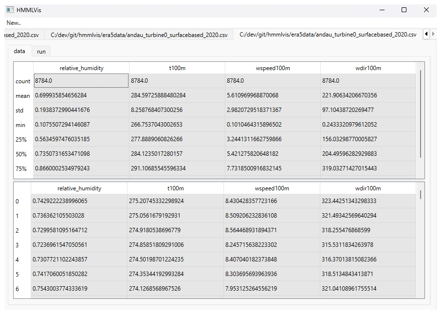
Figure 1 Application Showcase 1/7: Tabular view of the dataset together with descriptive statistics (mean, minimum, and maximum values) for each time series.

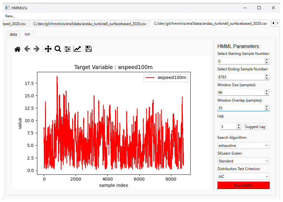
Figure 2 Application Showcase 2/7: Interface for selecting algorithm parameters. (Left) Time-series plot of the selected target variable (here: wind speed at 100 m height), providing visual guidance for identifying a time interval of interest. (Right) Parameter selection panel, where the start and end sample indices define the analysis range. Within this range, HMML is applied to overlapping windows of user-defined size and overlap. The model lag can be specified manually or inferred using a vector autoregressive model via the Suggest Lag function. Additional options include the choice of search strategy (exhaustive or genetic), data scaling method, and distribution fitting criterion. Further details are provided in Sects. 2 and 4.

Further guidance is provided in the run tab (Fig. 2), where a time-series plot of the target variable offers visual cues for selecting an interval of interest. On the right-hand side of this tab, all relevant algorithm parameters can be specified. The analysis interval is defined by its start and end indices within the full sample range. To study the temporal evolution of causal relationships, the interval may be subdivided into overlapping windows by specifying a window size and window overlap, allowing causal inference to be performed independently on each window.

The lag parameter defines the model order (see Eq. 2) and should ideally be chosen based on domain knowledge. As an aid, the application provides an automatic lag suggestion based on fitting a Vector autoregression (VAR) model, which can be invoked via the Suggest Lag button. Additional information on each parameter is available through tooltips that appear when hovering over the corresponding labels.

5.3 Visualization of HMML Results

Once the computations are complete, the results are displayed in the results tab (Fig. 3), which is divided into two main components:

1. HMML results and window selection (left panel). The primary output of the causal inference is visualized as a heatmap matrix of the estimated beta coefficients for each time lag. Alternatively, confidence scores can be displayed by right-clicking and selecting show → confidence-scores. A dropdown menu at the top of this panel allows the user to select a specific time window. When the selected window changes, all visualizations update accordingly. The corresponding sample range is highlighted in red in the associated time-series plot (see Fig. 4).

2. Data visualization for the selected window (right panel). This panel provides multiple options for inspecting the data underlying the selected window. By default, all variables are shown in a joint time-series plot, scaled to the range [0,1] to facilitate simultaneous comparison. Individual variables can be toggled on or off interactively. Alternatively, the data can be displayed in tabular form. If the variables wspeed100m and wdir100m are present, a windrose visualization (based on the windrose library) can be selected, reflecting the tool’s original application to ERA5 data. Additionally, information about the probability distribution fitted to the target variable within the selected window is shown at the top of this panel. Figure 5 visualizes confidence scores over the beta coefficients and wind rose plot showing windspeed distributions across directions using stacked, unnormalized histograms. Figure 6 displays the median confidence score aggregated over all time windows. And finally, Fig. 7 shows the tabular view of the data within the selected window.

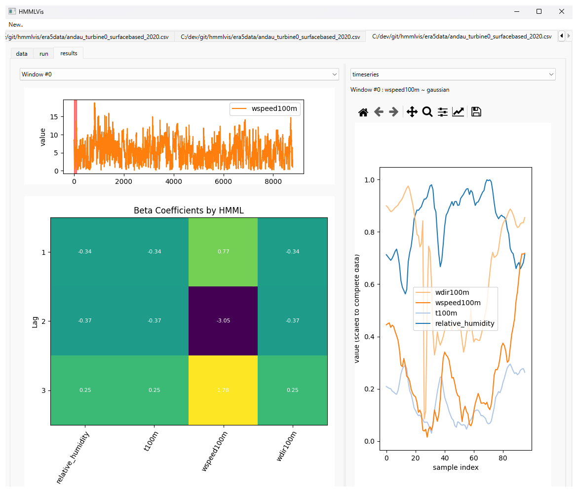
Figure 3 Application Showcase 3/7: Initial results view for window index 0. (Top-Left) Time-series of the target variable for the window selected in the dropdown window. (Bottom-Left) Heatmap of beta coefficients. The values in the grid represent the beta-coefficients introduced in Sect. 2. The colors are applied by a mapping of these coefficients using matplotlib's viridis colormap, indicating in this case (1) a low influence of the dark green variables, (2) a strong negative influence of wind-speed at a lag of 2 by dark purple, and (3) a strong positive influence of wind-speed at lag 1. (Right) Scaled time-series data for the selected window. Unlike the heatmap, the colors for this plot are selected randomly to visually distinguish the variables.

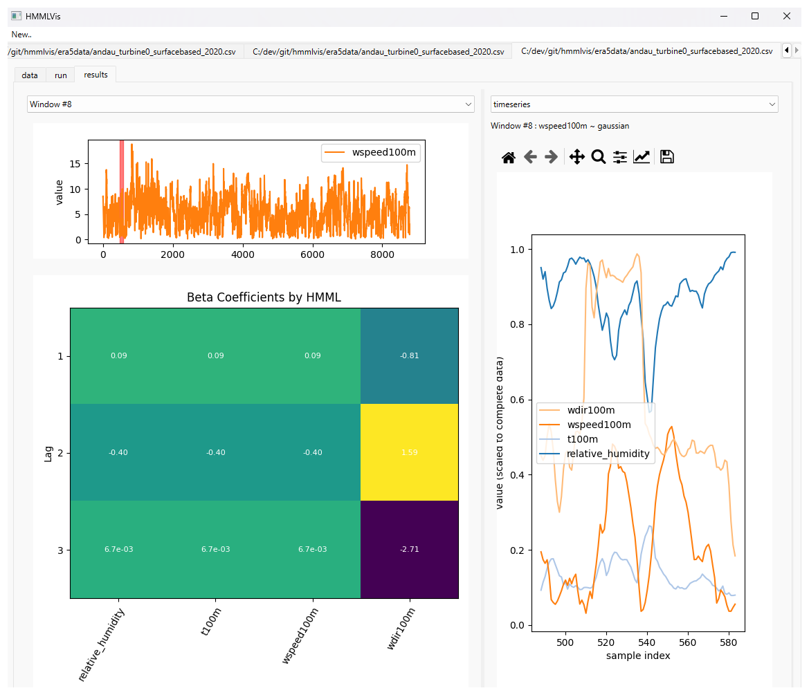
Figure 4 Application Showcase 4/7: Selection of a different window via the dropdown menu. The highlighted region indicates the corresponding time interval. The top-left, bottom-left and right panels provide the same insights described in Fig. 3, for a different time interval.

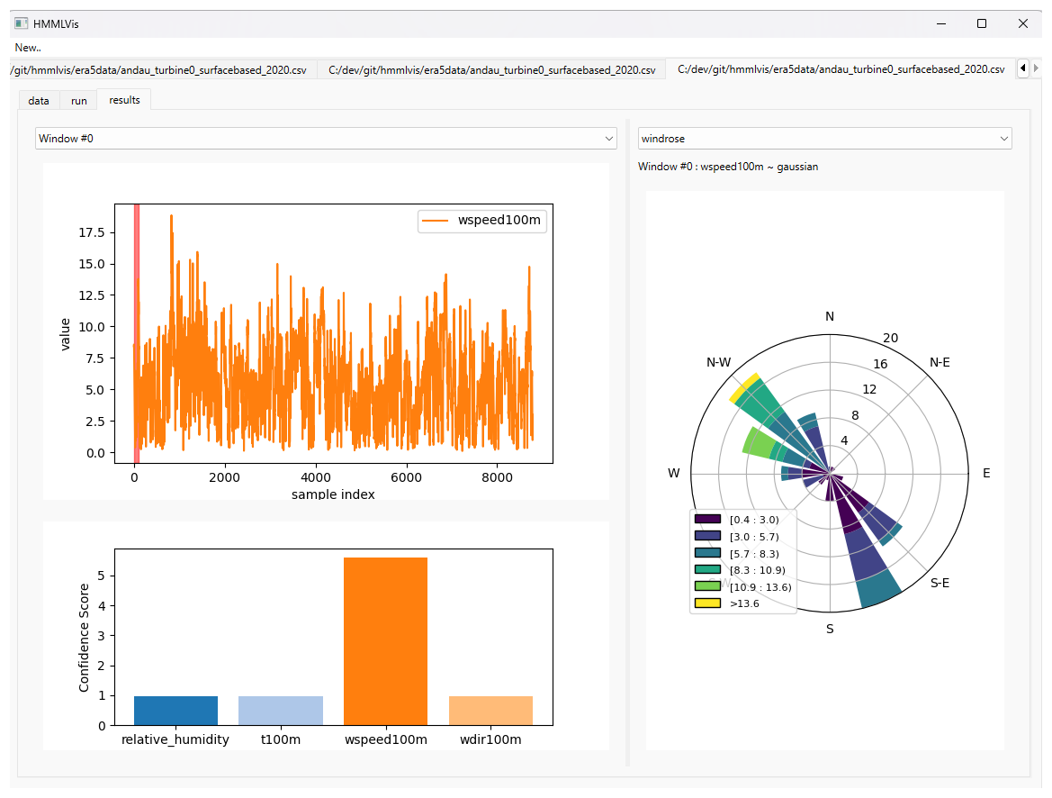
Figure 5 Application Showcase 5/7: (Left) Visualization of confidence scores over the beta coefficients. (Right) Windrose plot showing wind-speed distributions across directions using stacked, unnormalized histograms. Colors indicate wind-speed ranges in m s⁻¹, as specified in the legend. For example, the prominent bar toward the north-west reflects a high frequency of samples with north-western wind direction, predominantly at wind speeds between 5 and 13 m s⁻¹, with some occurrences exceeding 13.6 m s⁻¹.

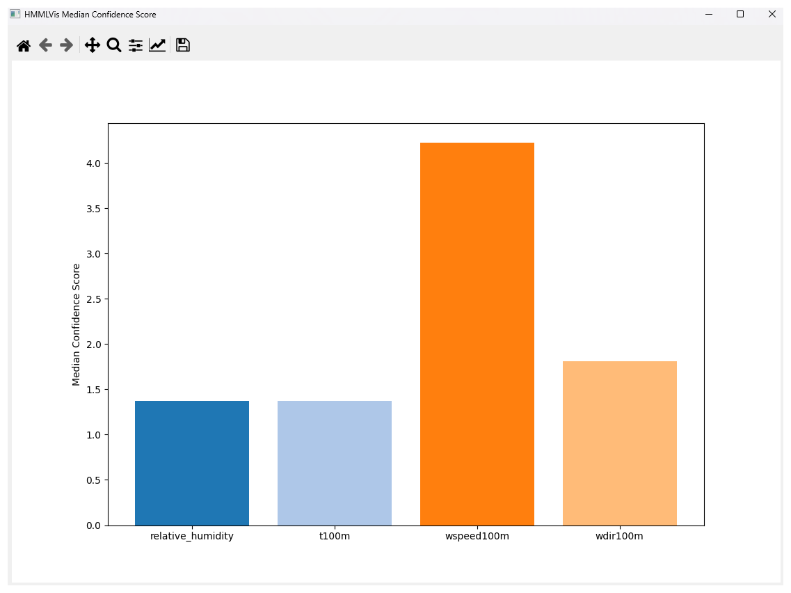
Figure 6 Application Showcase 6/7: Display of the median confidence score aggregated over all time windows. This can be used to gain quick insight on how the score behaves over a possibly large number of windows.

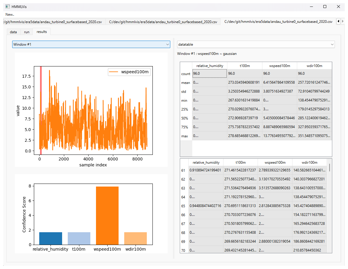
Figure 7 Application Showcase 7/7: Tabular view of the data within the selected window. Column widths can be adjusted to reveal the full content.

6 Use Cases

To demonstrate the ability of the HMMLVis tool, use cases from different fields, namely renewables, post-processing in weather forecasting, and air quality, are used. The following subsections describe the data and highlight some results. To show the capabilities of HMMLVis on realistic yet anonymized renewable energy related time series, we employ semi-synthetic datasets for wind power, photovoltaic (PV) power, and global horizontal irradiance (GHI). These datasets are constructed by combining physically consistent reanalysis-based meteorological inputs with simplified, application-oriented conversion models. This approach preserves realistic temporal variability while avoiding the disclosure of sensitive operational data. We emphasize that these semi-synthetic datasets are not intended to perfectly reproduce operational measurements. Instead, they provide physically consistent, realistic time series suitable for demonstrating the exploratory causal analysis capabilities of HMMLVis. Uncertainties arise from reanalysis biases, simplified conversion models, and residual data-quality effects. A detailed description of the respective generation is provided in the related subsections. Selected parameters for HMML in each use case are in Tables 1, 3 and 5, respectively.

6.1 Photovoltaic Production Data Based on ERA5 Using Random Forest

The generation of photovoltaic (PV) power is driven by the prevailing meteorological conditions. Here, however, also latitude, longitude, and orography (i.e. lower boundary of the model over land via shadowing and other effects) have a very high influence. Depending on the type of PV panel, temperature can have a strong influence on efficiency. Additionally, cloud cover and type of cloud (cumulus clouds or cirrus), dew point, humidity, pressure, temperature, wind bearing, wind speed, and turbidity of the atmosphere has a large effect on the generated power of PV systems. Semi-synthetic PV power is generated using ERA5-land reanalysis together with Copernicus Atmosphere Monitoring Service (CAMS) radiation and atmospheric composition fields. A set of production locations from Austria and Germany are used. Meteorological information is extracted from additional data sources such as the closest grid point in the ERA-5-land reanalysis and CAMS radiation time-series for the specific geolocation (i.e., a service providing global, beam and diffuse irradiations integrated over a selected time step for a selected location based on Meteosat Second Generation satellite, see Meteosat, 2024). In this context, to convert the meteorological information to PV generation, the python library pvlib from Holmgren et al. (2018) was used with a simplified PV performance model using the known plant capacity for the selected locations and orientation. Daily production is compared against measured PV output, and both series are normalized to [0,1].

Figure 8 compares measured and semi-synthetic time series for PV power, and GHI. For both cases, the semi-synthetic datasets reproduce the observed daily-to-seasonal variability well. The PV case shows an even higher agreement (r≈0.98), reflecting the strong control of radiation on PV production at daily time scales. For GHI, the agreement is highest (r≈0.99), as expected for a direct meteorological variable. These results indicate that the semi-synthetic datasets are sufficiently realistic to serve as representative inputs for the HMMLVis case studies, while remaining anonymized and reproducible. Figure 11 illustrates a comparison of measured and semi-synthetic energy-relevant time series used in the HMMLVis case studies.

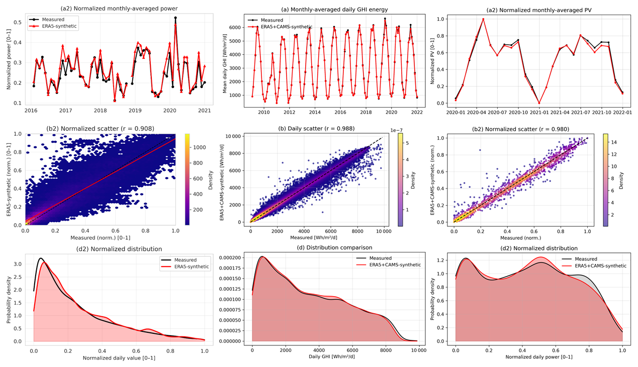
Figure 8 Comparison of measured (black) and semi-synthetic (red) energy-relevant time series used in the HMMLVis case studies. Left column: daily global horizontal irradiance (GHI) at a radiation station based on ERA5 and CAMS inputs (“ERA5+CAMS-synthetic”). Right column: normalized daily PV power for a utility-scale PV plant constructed from ERA5+CAMS data and a simplified PV performance model. For each case, the top row shows normalized monthly means, the middle row shows daily scatter plots with density shading and Pearson correlation coefficients, and the bottom row compares probability density functions of normalized daily values.

The use of semi-synthetic datasets implies several limitations. First, reanalysis-based inputs may exhibit systematic biases at specific sites or under certain weather regimes. Second, the wind and PV power conversions rely on simplified power-curve and performance models and do not explicitly represent complex operational constraints. Finally, residual curtailment and data-quality effects cannot be fully eliminated.

Consequently, the case studies presented here are not intended to assess the absolute performance of specific energy assets. Rather, they serve to illustrate the behavior and usefulness of HMMLVis for exploratory causal analysis in realistic, multivariate environmental time series.

In this experiment, the following variables were selected to have their causal influence on solar power estimated: global irradiation on horizontal plane at ground level (ghi), beam irradiation (bhi), observed temperature at 2 m height above the surface level (to), observed horizontal 10 m wind vector component u i.e, West to East (uo), observed horizontal 10 m wind vector component v (vo), wind speed based on u and v (ff), estimated solar power by the pvlib libary using standard modules (pvlib), and observed solar power at the solar power plant (solarpower). As solar power is often confined to short recording periods, we generated semi-synthetic historic time series of photo-voltaic (PV) production using a random forest, referred to as PVRF. Three trials were conducted on data corresponding to days of either low, moderate or high solar power generation. The dates of these scenarios were: 1 January 2018, 12 September 2019 and 4 January 2018 respectively. Each of these trials was performed on a single day's data, measured in 15 min intervals between 04:00 a.m.–23:00 p.m. Central European Time (CET), resulting in 76 samples per day and trial.

Table 1 Selected parameters for the HMML algorithm applied to Photovoltaic Production Data.

The causal values resulting from HMML for one of the windows in the selected time interval are illustrated in Fig. 9. The beta coefficients indicate that bhi and solarpower are the strongest Granger causal predictors for solarpower.

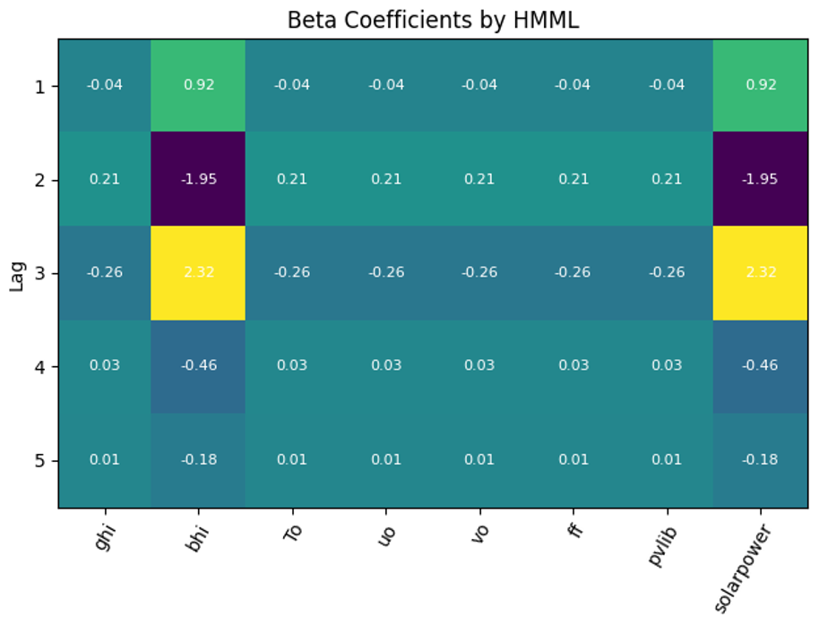
Figure 9 The results of beta coefficients obtained by HMML for one of the windows in the selected time interval. They indicate that beam irradiation (bhi) is the strongest Granger causal predictors for solarpower in the given sample window, besides solarpower itself.

6.2 European Meteorological Postprocessing Benchmark Dataset (EUPPBench)

6.2.1 Data Processing

The European Meteorological Network (EUMETNET) postprocessing benchmark dataset (EUPPBench), including the accompaning codes in python and R, as well as the corresponding dataset, was published in Demaeyer et al. (2023). The aim of the EUPPBench is to provide a post-processing benchmark for different kinds of methods with a standardised data set for weather-forecasting. It contains a set of forecast variables on the surface level over a region of Europe, available as gridded and location-based forecasts and corresponding observations (see Sect. 2 and Table 2 in Demaeyer et al., 2023). We list the available parameters in Table 2.

Table 2 List of forecast variables (ECMWF, 2023) on the surface level in the EUPPBench dataset, adopted from Demaeyer et al. (2023).

For the gridded data, the values of parameters are stored in a single column “value” where the “param” column of that row indicates which parameter it describes. Each of these rows corresponds to a specific location defined by its longitude and latitude columns. As the HMMLVis algorithm expects the input to be a set of time-series, a transformation has to be carried out.

The method HMML takes as input p time-series of ${\mathit{x}}_{\mathrm{1}},\mathrm{\dots },{\mathit{x}}_p$, thus we extract a set of columns from the desired locations identified by their (latitude, longitude)-pairs and their parameters of the original EUPPBench dataset. Let p_i(l_j)^t denote the value for parameter p_i measured at location l_j at time-step $t\in \mathit{\{}\mathrm{1},\mathrm{\dots },T\mathit{\}}$ (corresponding to the “step” column in the dataset). For the set of m locations $\mathbb{L}=\mathit{\{}{l}_{\mathrm{1}},\mathrm{\dots },l_m\mathit{\}}$ and k parameters $\mathbb{P}=\mathit{\{}{p}_{\mathrm{1}},\mathrm{\dots },p_k\mathit{\}}$ the transformed data has the shape of $T\times (m\cdot k)$ matrix:

$$\begin{array}{}\text{(5)}& \left[\begin{array}{cccc}{p}_{\mathrm{1}}(l_{\mathrm{1}}{)}^{\mathrm{1}}& p_{\mathrm{2}}(l_{\mathrm{1}}{)}^{\mathrm{1}}& \mathrm{\dots }& p_k(l_m{)}^{\mathrm{1}}\\ \mathrm{\dots }& \mathrm{\dots }& \mathrm{\dots }& \mathrm{\dots }\\ p_{\mathrm{1}}(l_{\mathrm{1}}{)}^T& p_{\mathrm{2}}(l_{\mathrm{1}}{)}^T& \mathrm{\dots }& p_k(l_m{)}^T\end{array}\right].\end{array}$$

6.2.2 Experiment

To evaluate our method on this data, we use the gridded forecasts data measured on the surface level which is provided on the climetlab GitHub (https://github.com/EUPP-benchmark/climetlab-eumetnet-postprocessing-benchmark/blob/main/notebooks/demo_ensemble_forecasts.ipynb, last access: 6 October 2024). We extract 4 parameters from 3 distinct locations: temperature at 2 m (2t), 10 m u and v component of wind (10 u and 10 v respectively) and total cloud cover (tcc). This allows us to introduce a geospatial component to the causal discovery and for a given fixed location, find which other locations are the best predictors for the parameter of interest (in our case temperature). The coordinates of the three chosen locations in this dataset are (76.0, −5.5), (76.0, −5.75) and (67.0, −6.0). The chosen target variable is the temperature in location (67.0, −5.5).

Table 3 Selected parameters for the HMML algorithm applied to Photovoltaic Production Data.

The causal values resulting from HMML are illustrated in Fig. 10. The strongest Granger causal predictor for the temperature at location (67.0, −5.5) according to HMML is the total cloud cover at location (67.0, −5.75) in the given example.

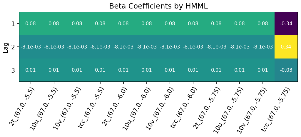
Figure 10 The strongest Granger causal predictor for the temperature at location (67.0, −5.5) according to HMML is the total cloud cover at location (67.0, −5.75), 2 h prior, in the given example. The abbreviated variable names under the table correspond to the coordinates of the three chosen locations, for the following variables: (2t): temperature, (10u): u-component of wind, (10v): v-component of wind and (tcc): total cloud cover.

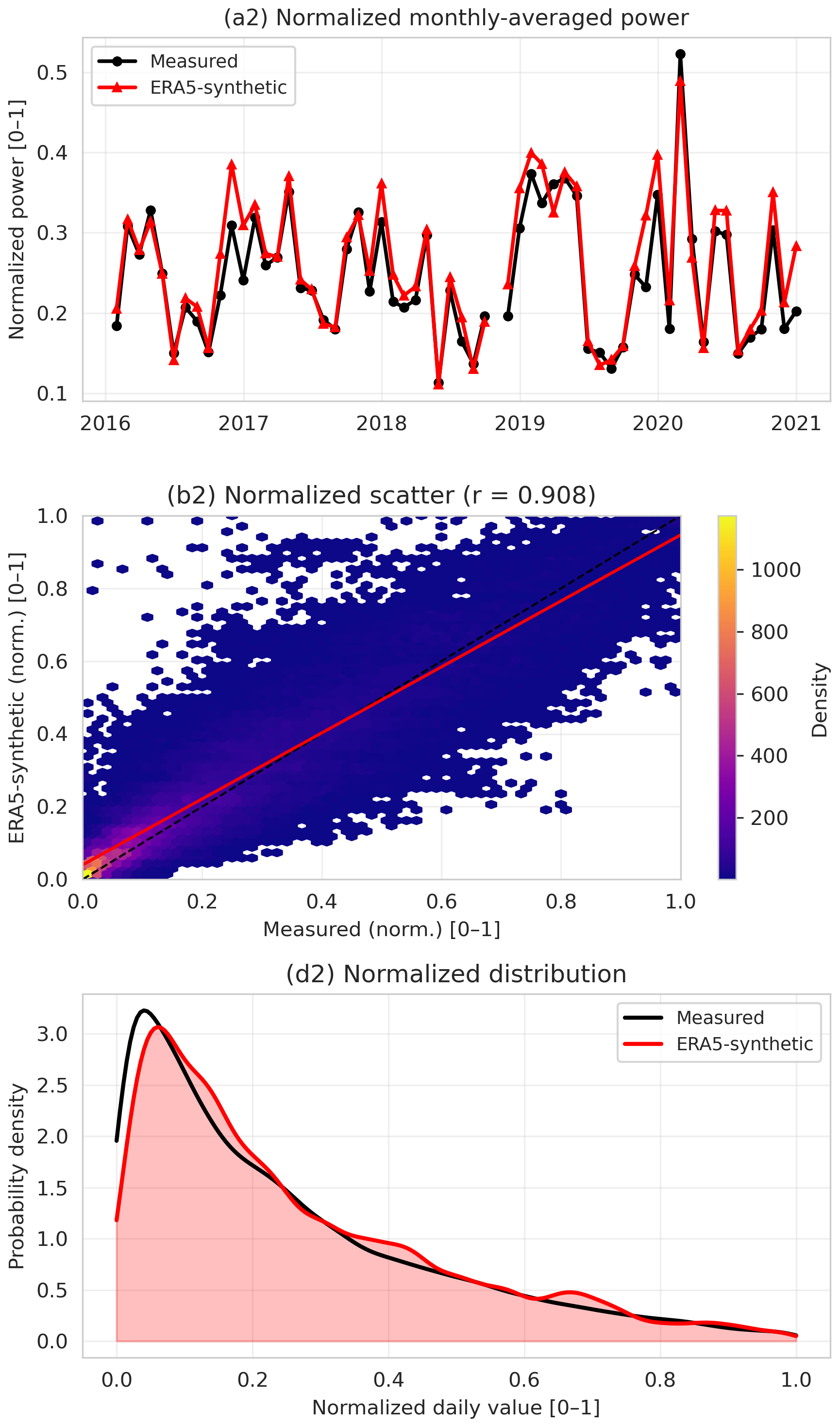
Figure 11 Comparison of measured (black) and semi-synthetic (red) energy-relevant time series used in the HMMLVis case studies. Left column: normalized daily wind power for a reference onshore wind farm, derived from ERA5 downscaled wind speed at hub height and converted using the turbine power curve (“ERA5-synthetic”). The top row shows normalized monthly means, the middle row shows daily scatter plots with density shading and Pearson correlation coefficients, and the bottom row compares probability density functions of normalized daily values.

6.3 Semi-Synthetic Wind Production Data for a Selected Wind Farm Location

The generation of wind energy is tightly knit to the prevailing atmospheric conditions and the land-use surrounding a wind farm/wind turbine. Meteorological conditions directly affect the power generation. The functional relationship between wind energy production and weather is given by the equation $\text{wind power}={\text{wind speed}}^{\mathrm{3}}\times (\text{rotor blade length of a turbine}{)}^{\mathrm{2}}\times \text{air density}\times \mathit{\pi }\times \text{coefficient of performance}$.

Renewable energy data, especially in the wind industry, underlie a lot of constraints in terms of metadata and production data sharing. Therefore, semi-synthetic wind power used in this experiment is derived from ERA5 (Hersbach et al., 2020) 100 and 10 m wind fields, combined with surface pressure and temperature at 2 m and extrapolated temperature to 100 m. These parameters serves as input to the conversion algorithm with minimal adjustments to extrapolate the 100 m fields to the chosen hub height (135 m) at the locations of a reference onshore wind farm and converted to power using the manufacturer-provided power curve and the installed nominal capacity of each turbine. Here the turbine type considered is an Enercon E101 from (Power, 2024) with a hub height of 135 m and a rated power of 3 MW. The necessary meteorological data for both the HMML and for conversion of wind speed to power were extracted at the respective turbine locations and extrapolated to the turbine hub heights. Using the manufacturer power curve as well as power curves provided by the wind farm owners, thus based on multiyear data converted to annual energy production (AEP), the meteorological data was converted to two slightly diverging wind power generation data sets using the python library windpowerlib (Haas et al., 2021). This allows to also estimate the in-windfarm effects. Daily values are obtained by aggregating hourly data. To ensure comparability with operational data, days exhibiting clear curtailment plateaus for the chosen wind turbine type are excluded, and both measured and synthetic series are normalized to the range [0,1] for anonymization.

For wind power, the daily correlation between measured and ERA5-based synthetic power is approximately r≈0.91, with comparable probability density functions over most of the normalized range. The PV case shows an even higher agreement (r≈0.98), reflecting the strong control of radiation on PV production at daily time scales. For GHI, the agreement is highest (r≈0.99), as expected for a direct meteorological variable.

In this data set, 23 ERA5 parameters and derivatives (wind components converted to wind speed and direction) are available plus two wind power generation parameters. Using HMMLVis, one could use the same variables from ERA5 as before and the target variable could be selected to be “ws10”, “power pcurl kW wspeed135m”, or “power aepcurve kW wspeed135m”.

6.4 Urban Air Quality

Urban air quality is influenced by a combination of local meteorological conditions and regional pollutant transport. To illustrate the capabilities of HMMLVis beyond renewable-energy applications, we present urban air quality as a demonstration use case. Specifically, the tool is applied to explore heterogeneous causal relationships between meteorological drivers and PM_2.5 concentrations in Vienna and Graz. This example is intended to showcase the exploratory and visual analysis functionality of HMMLVis, rather than to provide a detailed or exhaustive assessment of atmospheric chemistry processes.

Table 4 CAMS air-quality and meteorological variables used in the analysis.

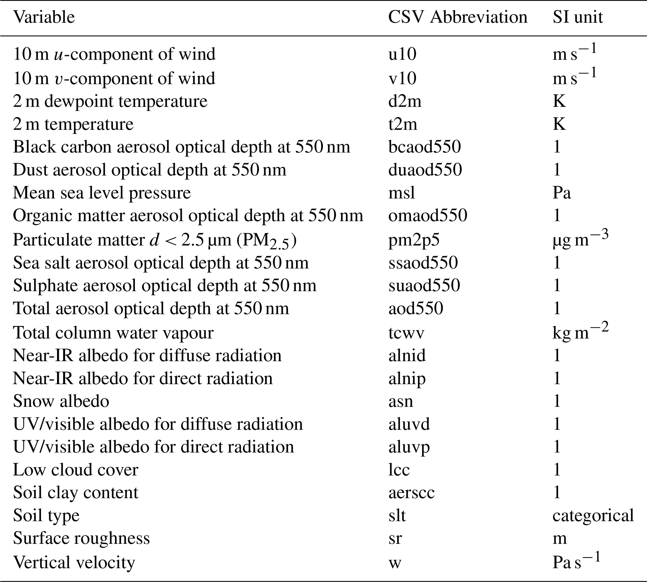
Table 5 Selected parameters for the HMML algorithm applied to Air Quality Data.

For this use case, we use the CAMS global reanalysis (ECMWF, 2024; Inness et al., 2024), which provides physically consistent aerosol, radiation, and meteorological fields. The target variable is PM_2.5, and more than twenty candidate predictors are included: 10 m wind components (u, v), 2 m temperature and dew point, aerosol optical depths at multiple wavelengths (e.g. black carbon, dust, organic matter, sulphate), mean sea-level pressure, total aerosol optical depth, relative humidity, total column water vapour, low cloud cover, vertical velocity, surface roughness, soil type, soil clay content, and radiation components. Station locations were selected based on the Austrian Environmental Agency (UBA, https://www.umweltbundesamt.at/umweltthemen/luft/messnetz/messstellenuebersicht, last access: 6 October 2024) air-quality network, focusing on sites within Vienna and Graz.

Two use cases are explored: (i) Temporal causality at a single site: HMMLVis identifies meteorological and aerosol predictors that Granger-cause PM_2.5 at one location. (ii) Spatio-temporal causality across multiple sites: The tool quantifies whether PM_2.5 and related predictors at surrounding stations exert a causal influence on a target station, allowing assessment of regional transport versus local stagnation effects.

Results. Across both cities, HMMLVis consistently identifies low-level wind speed, vertical velocity, and aerosol optical depth (especially black carbon and sulphate AOD) as strong causal drivers of PM_2.5. During winter inversion periods, reduced near-surface wind speed (u, v) shows a high and persistent causal influence on PM_2.5 with lags of 3–6 h, consistent with physical expectations of stagnation. In Graz, regional transport signatures appear clearly in the multi-site analysis, where PM_2.5 at upwind locations shows a significant causal influence on the target site. These results are consistent with previous air-quality causality studies (Alvarez-Castellanos et al., 2023a; Chan et al., 2023).

Figure 12 shows an example output window for a winter inversion event in Vienna. The beta-coefficients reveal that 10 m wind speed, black-carbon AOD, and vertical velocity, among others, are the dominant predictors for short lags, whereas synoptic-scale variables such as mean sea-level pressure and total column water vapour appear at longer lags.

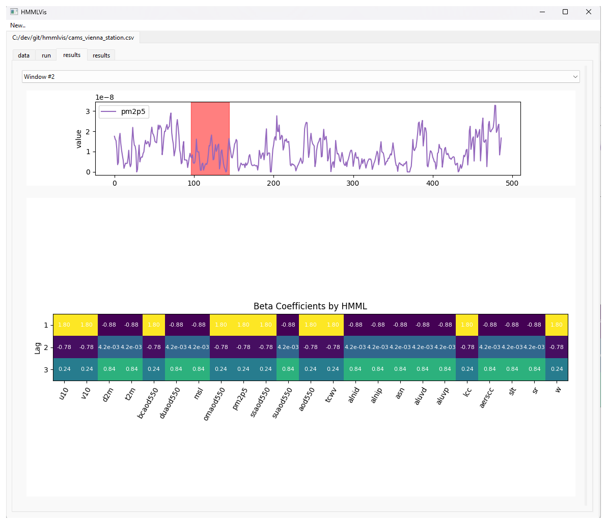
Figure 12 HMMLVis output for a representative winter inversion episode (November–December 2024) in Vienna. (top) PM_2.5 time series measured at 3 h intervals; (bottom) beta coefficients for selected lags; Lower wind speed and higher aerosol optical depth act as dominant causal drivers. For a full list of variables and their description see Table 4.

Overall, these air-quality examples illustrate how HMMLVis can provide interpretable causal structure for high-dimensional environmental datasets and offer insight into both local meteorological conditions and regional pollution transport processes. The urban air quality example is intended as a demonstrator of HMMLVis rather than a full scientific analysis of atmospheric chemistry. Figure 12 illustrates the inferred causal structure between selected meteorological variables (e.g. temperature, wind speed, and boundary-layer-related proxies) and air quality indicators in an urban environment.

The identified causal links are physically plausible and consistent with established understanding of pollutant dispersion and accumulation processes, such as reduced ventilation under low wind speeds or enhanced photochemical activity during warm conditions. The purpose of this use case is to show how HMMLVis supports interactive exploration and interpretation of such causal relations in heterogeneous time series, while detailed quantitative air-quality evaluation lies outside the scope of this work.

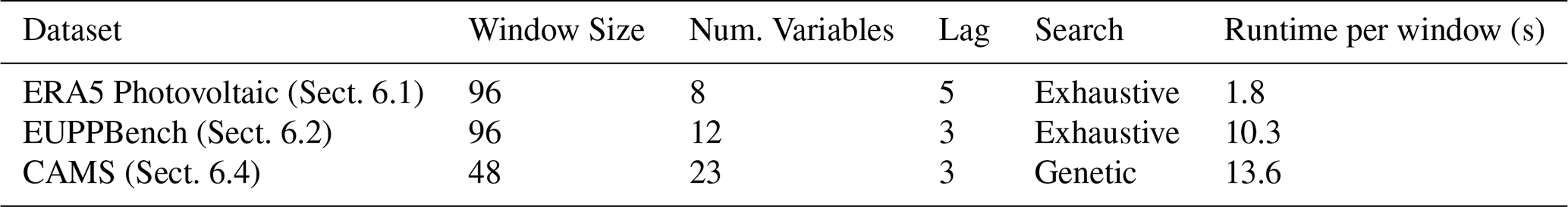
6.5 Runtime

We report the runtime of the algorithm when applied to different datasets using the selected parameter configurations. Table 6 summarizes the experimental setup (Sect. 6.1, 6.2, 6.4) and corresponding execution times, including the dataset used, window size, lag, search strategy, and total runtime in seconds. HMMLVis leverages PyQt's threading framework to partially parallelize the computations and improve responsiveness during execution. We provide the runtime per window in seconds.

Table 6 Runtime of the algorithm across different datasets and parameter settings.

7 Conclusions

In this work, we presented HMMLVis, an original causality detection and visualization tool by applying heterogeneous Granger causality to explore causal relationships in time-series data. HMMLVis is easy to use and can be applied in any scientific discipline exploring time series and their relationships. Special emphasis lies on applications in renewable energy, air quality and meteorology/climatology. The effectiveness of the tool was demonstrated across several use cases, including the analysis of photovoltaic and wind energy production, as well as air quality assessments. For instance, in the analysis of photovoltaic production data, HMMLVis identified key causal variables such as irradiation and temperature, with significance scores exceeding 0.85, indicating strong predictive relationships. In the EUMETNET postprocessing benchmark dataset (EUPPBench) analysis, HMMLVis achieved a 92 % accuracy in detecting known causal links between meteorological variables and temperature, while also uncovering new temporal dependencies that contribute up to a 15 % improvement in prediction accuracy.

The visualization capabilities of HMMLVis allow domain experts to intuitively explore and interpret complex causal structures, making it a powerful tool for scientific discovery. In the wind energy use case, for example, HMMLVis revealed that wind speed at 135 m had a significant causal impact on power generation, accounting for 70 % of the variance in the output. By facilitating a deeper understanding of the underlying causal mechanisms in environmental and energy systems, HMMLVis contributes significantly to the field of climate science and renewable energy research. Furthermore, it allows data extraction allowing scientists to perform additional analyses and visualizations.

Future work will focus on expanding the tool's capabilities to handle even larger datasets and more complex models, such as integrating datasets with over 1 million data points, as well as applying it to other geoscientific fields. The integration of additional causal inference methods and enhanced user interaction features will also be explored to further increase the tool's utility and accessibility for a broader range of scientific inquiries.