A fully implicit second order method for viscous free surface Stokes flow – application to glacier simulations

We present a fully implicit finite element method for viscous free surface Stokes problems which are common in glaciology and geodynamics. Standard fully implicit iterative solvers diverge for such problems when using large time steps. We address this by incorporating a stabilization term that vanishes upon convergence. This approach enables the use of large time steps, thereby significantly improving the efficiency of simulations. Furthermore, we leverage the fully implicit solver to develop second-order time-stepping schemes that mitigate the high errors associated with first-order methods for large time steps. The methods are tested and evaluated on model domains relevant to geodynamics and glaciology.

1 Introduction

Viscous, gravity-driven, free surface problems are prevalent in geoscientific applications such as mantle convection and glaciology (Greve and Blatter, 2009; Rose et al., 2017). Such simulations involve solving the Stokes equations for the velocity and pressure, ($\mathit{u}(x,y,z,t)$, $p(x,y,z,t)$), and a free-surface equation for the upper surface height $h(x,y,t)$ that determines the geometry, see Fig. 1. A key computational challenge arises from the strong coupling between the evolving geometry and the velocity field, which can lead to numerical stability issues and imposes severe restrictions on the time-step size, ultimately reducing computational efficiency. Fully implicit methods would overcome these time-step limitations, but the strong coupling introduces convergence issues that prevent practical usage.

In ice-sheet and glacier modeling, the time-step size restriction is a prominent problem (Cheng et al., 2017; Löfgren et al., 2022, 2024). Ice-sheet and glacier models describe the movement of the ice covering Antarctica and Greenland, or that of smaller mountain glaciers and ice caps. Under the long time scales that are relevant to ice dynamics, ice deforms as a viscous fluid. It slowly creeps under its own weight from the interior of a continent to the coast, where it melts due to lower altitudes and meeting the warm ocean. Accurately calculating the geometry and the rate of flow towards the ocean is crucial in estimating the future rise in sea level in response to climate change. However, the computational challenges of ice-sheet modeling limit the accuracy of projections (Pörtner et al., 2019). Due to the coupling between geometry and ice velocity, the full problem can be likened to solving the heat equation, but the state-of-the-art numerical methods are explicit in time. To maintain stability, time-steps are therefore often limited to around 0.1–1.0 years (Leguy et al., 2021), which is a bottleneck. Implicit iterations would increase the largest stable time-steps but are challenging and have so far only been achieved for approximate models (Bueler, 2016). For models based on the full Stokes equations there is, to our knowledge, no working implicit method based on iterations. A monolithic implicit solver was constructed in Kramer et al. (2012) for geodynamics. The great promise of implicit methods was recognized by Bueler (2022) who later conjectured that such schemes should be well-posed (Bueler, 2024).

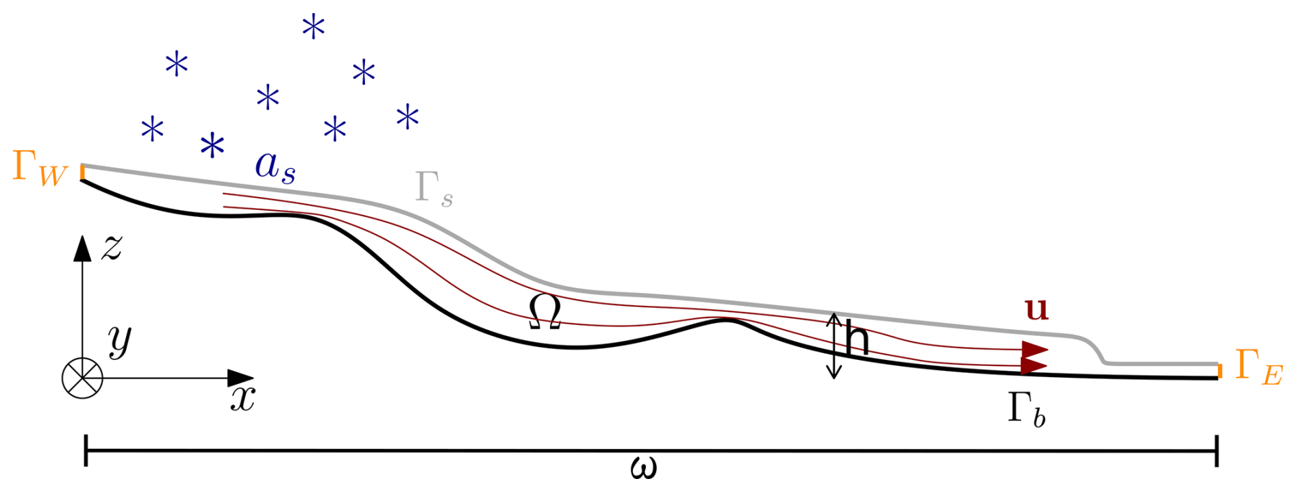
Figure 1 Illustration of a viscous free surface problem in the form of a mountain glacier. The ice is formed by accumulated snow and flows down the mountain due to the force of gravity. The surface height h indicates the distance from z=0 to the surface Γ_s. The domain ω is the projection of the full domain Ω from ℝ^d to ℝ^d−1. The vertical position of the line |———–| used to denote ω is arbitrary chosen. Adapted from Löfgren et al. (2024), published in The Cryosphere, licensed under CC BY 4.0.

In this paper, we present a numerically stable and accurate fully implicit method by introducing boundary terms in the Stokes equations, which vanish during convergence. We argue that the convergence issues of standard implicit iterations are connected to the stability issues that are seen for explicit methods (since the first iteration has to be explicit), and we introduce a method that circumvents these issues in a computationally efficient way. The method relies on the Free Surface Stabilization Algorithm (FSSA), which was originally developed for mantle convection problems (Kaus et al., 2010) and later adapted for ice sheet simulations (Löfgren et al., 2022, 2024). The FSSA relaxes the time-step restrictions for explicit solvers by adding additional boundary terms. We adapt this method to the context of fully-implicit solvers. The boundary terms vanish as convergence is reached. This method allows for very large time-steps and ensures consistency. We then utilize the new implicit method to construct second-order accurate time-stepping schemes and demonstrate efficiency and accuracy on setups relevant to geodynamics and glacier simulations.

2 Governing equations and their finite element discretization

The surface height position h, the velocity $\mathit{u}=(u_x,u_y,u_z)$ and the pressure p are the solution to a system of coupled partial differential equations, namely the 𝔭-Stokes-coupled free-surface equation:

$$\begin{array}{}\text{(1)}& {\displaystyle }& {\displaystyle }\left.\begin{array}{ll}-\mathrm{\nabla }\cdot \mathbf{S}\left(\mathbf{D}\mathit{u}\right)+\mathrm{\nabla }p& =\mathit{\rho }\mathit{g},\\ \mathrm{\nabla }\cdot \mathit{u}& =\mathrm{0}\end{array}\right\}\mathrm{in}\mathrm{\Omega }\left(t\right),\text{(2)}& {\displaystyle }& {\displaystyle \frac{\partial h}{\partial t}}+\mathit{u}(x,y,z=h,t)\cdot \mathrm{\nabla }h=a_{\mathrm{s}}\mathrm{on}\mathit{\omega }.\end{array}$$

Here, Ω⊂ℝ^d with $d\in \mathit{\{}\mathrm{2},\mathrm{3}\mathit{\}}$, is an open and bounded domain with a boundary Γ, of which one part is the upper free surface Γ_s which is located at a height h, see Fig. 1 for an illustration from glaciology. The free-surface equation (Eq. 2) is solved on $\mathit{\omega }\in {\mathbb{R}}^{\mathrm{d}-\mathrm{1}}$, which represents a projection of the upper ice surface Γ_s onto a flat two-dimensional plane. The ice-flow dynamics are driven by the gravitational term ρg. The free-surface equation can be forced by the term a_s, which in a glaciological context represents accumulation and ablation. The deviatoric stress tensor S depends on the strain-rate tensor $\mathrm{2}\mathbf{D}\mathit{u}=\mathrm{\nabla }\mathit{u}+(\mathrm{\nabla }\mathit{u}{)}^T$ according to a constitutive law

$$\begin{array}{}\text{(3)}& \mathbf{S}\left(\mathit{u}\right)=\mathit{\nu }\left(\mathbf{D}\mathit{u}\right)\mathbf{D}\mathit{u},\end{array}$$

where

$$\begin{array}{}\text{(4)}& \mathit{\nu }:=\mathit{\nu }\left(\mathbf{D}\mathit{u}\right)={\mathit{\nu }}_{\mathrm{0}}{\left({\mathit{\epsilon }}^{\mathrm{2}}+|\mathbf{D}\mathit{u}{|}^{\mathrm{2}}\right)}^{\frac{\mathfrak{p}-\mathrm{2}}{\mathrm{2}}}\mathfrak{p}\in (\mathrm{1},\mathrm{2}],\end{array}$$

is the viscosity function, dependent on the effective strain rate $\left|\mathbf{D}\mathit{u}\right|$; ε² is a regularisation term to avoid infinite viscosity at zero shear strain rate. The relation is linear for 𝔭=2, as for Newtonian dynamics and non-linear for non-Newtonian materials such as glacial ice for which $\mathfrak{p}=\mathrm{4}/\mathrm{3}$, where 𝔭 is usually stated in terms of the Glen's parameter $n=\mathrm{1}/(\mathfrak{p}-\mathrm{1})$. We consider a very viscous flow, so that ν₀ is large.

A key challenge in the time discretization of such problems arises from the fact that the computational domain Ω is coupled to the time-dependent height of the ice surface $h(x,y,t)$ so that Ω(t)=Ω(h(t)). The dependence of the domain on the surface elevation h means that the velocity field also implicitly depends on h. At the same time, these velocity components appear as coefficients in the free surface evolution equation that governs the changes in h. The mutual dependence between h and u limits the numerical stability of explicit methods.

The Stokes equations are solved under the following boundary conditions: At the top surface Γ_s a stress-free boundary condition is applied

$$\begin{array}{}\text{(5)}& \left(\mathbf{S}\right(\mathbf{u})-\mathbf{I}p)\cdot \mathit{n}=\mathbf{0}\mathrm{on}{\mathrm{\Gamma }}_{\mathrm{s}}.\end{array}$$

Here, $\mathit{n}=(n_x,n_y,n_z$) denotes the outward pointing normal and I the identity matrix. The lateral boundaries, Γ_W and Γ_E (see Fig. 1), are assumed to be rigid in this study so that an impenetrability condition applies,

$$\begin{array}{}\text{(6)}& \mathit{u}\cdot \mathit{n}=\mathrm{0},\mathrm{on}{\mathrm{\Gamma }}_{\mathrm{W}}\cup {\mathrm{\Gamma }}_{\mathrm{E}}.\end{array}$$

Lastly, at the base or bedrock, Γ_b, we apply either a no-slip condition

$$\begin{array}{}\text{(7)}& \mathit{u}=\mathbf{0}\mathrm{on}{\mathrm{\Gamma }}_{\mathrm{b}},\end{array}$$

or an impenetrability condition combined with a so-called Weertman sliding law

$$\begin{array}{}\text{(8)}& {\mathit{t}}_i\cdot \left(\mathit{\sigma }\mathit{n}\right)=-C\mathit{u}\cdot {\mathit{t}}_i\mathrm{on}{\mathrm{\Gamma }}_{\mathrm{b}},\end{array}$$

where t_i are tangent vectors that span the lower ice surface and C is the friction coefficient. Note that the methods in this article are not restricted to the specific boundary conditions on Γ_b, Γ_W and Γ_E.

We consider a finite element discretization in space, which is commonly used in both ice sheet modeling and geodynamics (Gagliardini et al., 2013; Larour et al., 2012; Kaus et al., 2010; Rose et al., 2017). The weak formulation of the Stokes problem is to find the velocity and pressure ($\mathit{u},p)\in [W_{\mathrm{0}}^{\mathrm{1},\mathfrak{p}}\left(\mathrm{\Omega }\right){]}^{\mathrm{d}}\times L^{{\mathfrak{p}}^{\prime }}\left(\mathrm{\Omega }\right)$ so that

$$\begin{array}{}\text{(9)}& \begin{array}{rl}\left(\mathbf{S}\right(\mathit{u}),\mathbf{D}\mathit{v}{)}_{\mathrm{\Omega }}& -(\mathrm{\nabla }\cdot \mathit{v},p{)}_{\mathrm{\Omega }}-(\mathrm{\nabla }\cdot \mathit{u},q{)}_{\mathrm{\Omega }}=(\mathit{\rho }\mathit{g},\mathit{v}{)}_{\mathrm{\Omega }}\forall (\mathit{v},q)\\ & \in {\left[W_{\mathrm{0}}^{\mathrm{1},\mathrm{p}}\left(\mathrm{\Omega }\right)\right]}^{\mathrm{d}}\times L^{{\mathfrak{p}}^{\prime }}\left(\mathrm{\Omega }\right),\end{array}\end{array}$$

where $(\cdot ,\cdot {)}_{\mathrm{\Omega }}$ denotes the L² scalar product, e.g. $(\mathit{u},\mathit{v}{)}_{\mathrm{\Omega }}=\underset{\mathrm{\Omega }}{\int }\mathit{u}\cdot \mathit{v}\mathrm{d}x$. The appropriate spaces for the continuous problem are the Sobolev space $\left[W_{\mathrm{0}}^{\mathrm{1},\mathfrak{p}}\right(\mathrm{\Omega }){]}^{\mathrm{d}}$ and the Lebesgue space $L^{{\mathfrak{p}}^{\prime }}\left(\mathrm{\Omega }\right)$, where ${\mathfrak{p}}^{\prime }=\mathfrak{p}/(\mathfrak{p}-\mathrm{1})$ (e.g., Hirn, 2013).

In this work, we discretize the weak form using Taylor-Hood (Taylor and Hood, 1974) elements, i.e. linear elements for the pressure and quadratic elements for the velocity. Such a discretization is inf-sup stable (Brezzi and Fortin, 1991).

The weak form of the free surface equation is to find the surface height $h\in W^{\mathrm{1},\mathrm{2}}\left(\mathit{\omega }\right)$ such that

$$\begin{array}{}\text{(10)}& {\left({\displaystyle \frac{\partial h}{\partial t}},q\right)}_{\mathit{\omega }}={\left(\left(-u_x{\displaystyle \frac{\partial h}{\partial x}}-u_y{\displaystyle \frac{\partial h}{\partial y}}+u_z\right),q\right)}_{\mathit{\omega }},\forall q\in W^{\mathrm{1},\mathrm{2}}\left(\mathit{\omega }\right).\end{array}$$

In this paper, it is useful to note that the equation can be written equivalently as

$$\begin{array}{}\text{(11)}& {\left({\displaystyle \frac{\partial h}{\partial t}},q\right)}_{\mathit{\omega }}=\underset{{\mathrm{\Gamma }}_{\mathrm{s}}}{\int }\mathit{u}\cdot \mathit{n}q\mathrm{d}s.\end{array}$$

The equivalence is easily seen by changing from integration on the surface to the two-dimensional footprint ω, and considering that the normal vector pointing out of a surface is $\mathit{n}=\stackrel{\mathrm{̃}}{\mathit{n}}/\Vert \mathit{n}\Vert$, where $\stackrel{\mathrm{̃}}{\mathit{n}}=(-{\partial }_{x}h,-{\partial }_{y}h,\mathrm{1})$. This derivation takes the form

$$\begin{array}{}\text{(12)}& \begin{array}{rl}(\mathit{u}& \cdot \mathit{n},q{)}_{{\mathrm{\Gamma }}_{\mathrm{s}}}=\underset{{\mathrm{\Gamma }}_{\mathrm{s}}}{\int }\mathit{u}\cdot \mathit{n}q\mathrm{d}s=\underset{\mathit{\omega }}{\int }\mathit{u}\cdot \mathit{n}q\sqrt{\mathrm{1}+{\left({\partial }_{x}h\right)}^{\mathrm{2}}+{\left({\partial }_{y}h\right)}^{\mathrm{2}}}\mathrm{d}x\\ & =\underset{\mathit{\omega }}{\int }\mathit{u}\cdot \left(-{\partial }_{x}h,-{\partial }_{y}h,\mathrm{1}\right){\displaystyle \frac{\mathrm{1}}{\sqrt{\mathrm{1}+{\left({\partial }_{x}h\right)}^{\mathrm{2}}+{\left({\partial }_{y}h\right)}^{\mathrm{2}}}}}q\\ & \sqrt{\mathrm{1}+{\left({\partial }_{x}h\right)}^{\mathrm{2}}+{\left({\partial }_{y}h\right)}^{\mathrm{2}}}\mathrm{d}x=\underset{\mathit{\omega }}{\int }\mathit{u}\cdot \left(-{\partial }_{x}h,-{\partial }_{y}h,\mathrm{1}\right)q\mathrm{d}x\\ & =\underset{\mathit{\omega }}{\int }{\displaystyle \frac{\partial h}{\partial t}}q\mathrm{d}x.\end{array}\end{array}$$

The free surface equation is discretized using linear elements.

3 Low-order time-stepping schemes and the free surface stabilization algorithm

The standard approach to solving the coupled system (Eqs. 1 and 2) is to solve the Stokes equations once per time step on a mesh that reflects the geometry from the preceding step, (Algorithm 1). An explicit Euler discretization of the free surface can thus be written as

$$\begin{array}{}\text{(13)}& \begin{array}{rl}{\left(h^{k+\mathrm{1}},q\right)}_{\mathit{\omega }}& ={\left(h^k,q\right)}_{\mathit{\omega }}+\mathrm{\Delta }t{\left(\left(-u_x^k{\displaystyle \frac{\partial h^k}{\partial x}}-u_x^k{\displaystyle \frac{\partial h^k}{\partial x}}+u_z^k\right),q\right)}_{\mathit{\omega }}\\ & ={\left(h^k,q\right)}_{\mathit{\omega }}+\mathrm{\Delta }t\underset{{\mathrm{\Gamma }}_{\mathrm{s}}^k}{\int }{\mathit{u}}^k\cdot {\mathit{n}}^{k}q\mathrm{d}{s}^k,\forall q\in W^{\mathrm{1},\mathrm{2}}\left(\mathit{\omega }\right),\end{array}\end{array}$$

where k is the current time step and k+1 is the next time step. In this explicit Euler discretization, the velocity, u, is, by necessity, always evaluated on time step k. It is easy to change to an implicit treatment of the surface height, h, by evaluating it at step k+1 instead, but as was shown in Löfgren et al. (2022, 2024), it is the treatment of the velocity u that determines the stability properties of the overall system. The explicit treatment of velocities is essentially analogous to solving the heat equation using an explicit Euler time-stepping scheme, and therefore, the time-step size is limited by stability constraints rather than by accuracy considerations.

Algorithm 1 Standard explicit ice sheet model algorithm.

1:

Create mesh

2:

for each time-step k do

3:

Solve Stokes Eq. for (u^k, p^k)

4:

Solve free surface equation for h^k+1

5:

Update mesh to get ${\mathrm{\Omega }}_{\mathrm{h}}^{k+\mathrm{1}}$

6:

end for

To avoid the restriction on the time-step, an implicit solver could in theory be used. A natural approach to such a solver is to iterate between the free surface solver and the Stokes solver until convergence. Unfortuntaely, the iterations do not converge for large time-steps. Here we adress this issue.

To relax the stability restriction without implicit iterations, the FSSA method was introduced in geodynamics in Kaus et al. (2010) and subsequently adapted to ice-sheet modeling in Löfgren et al. (2022, 2024). One way of understanding the FSSA stabilization method is by applying the Reynolds transport theorem to the gravitational force on weak form, assuming that $\frac{\partial }{\partial t}(\mathit{\rho }g\cdot \mathit{v})=\mathrm{0}$, which leads to:

$$\begin{array}{}\text{(14)}& {\displaystyle \frac{\partial }{\partial t}}\underset{\mathrm{\Omega }\left(t\right)}{\int }\mathit{\rho }\mathit{g}\cdot \mathit{v}\mathrm{d}\mathit{x}=\underset{\partial \mathrm{\Omega }\left(t\right)}{\int }\mathit{\rho }\left(\mathit{u}\right(t)\cdot \mathit{n}(t\left)\right)(\mathit{g}\cdot \mathit{v})\mathrm{d}s.\end{array}$$

An explicit Euler discretization of the above relation gives an expression for how the driving stress on time-step k+1 relates to the driving stress on time-step k:

$$\begin{array}{}\text{(15)}& \begin{array}{rl}\underset{\partial \mathrm{\Omega }\left(t^{k+\mathrm{1}}\right)}{\int }\mathit{\rho }\mathit{g}& \cdot \mathit{v}\mathrm{d}\mathit{x}\approx \underset{\mathrm{\Omega }\left(t^k\right)}{\int }\mathit{\rho }\mathit{g}\cdot \mathit{v}\mathrm{d}\mathit{x}\\ & +\underset{\mathrm{stabilization}}{\underbrace{\mathrm{\Delta }t\underset{\partial \mathrm{\Omega }\left(t^k\right)}{\int }\mathit{\rho }(\mathit{u}\cdot \mathit{n})(\mathit{g}\cdot \mathit{v})\mathrm{d}s}},\end{array}\end{array}$$

where the last term is the FSSA stabilization term. Note that the original FSSA method of (Kaus et al., 2010) includes a parameter θ in front of the stabilization term which will not be used here. The stabilization is added to the Stokes equations (Eq. 1) rather than the free-surface equation (Eq. 2). Due to the impenetrability condition, the FSSA term vanishes on all surfaces except Γ_s. Since the flow is gravity driven, it appears to be sufficient to represent the force of gravity implicitly (which FSSA does approximately) to yield an implicit solution. Note, however, that it is not a true fully implicit solver. The FSSA method has proved remarkably successful in increasing the largest stable time step in marine ice sheet models, by up to a factor of approximately 100 (Henry et al., 2025).

An observation that will be useful for creating the fully implicit solver is that the FSSA term is similar to the right-hand side of the discretized free surface equation (Eq. 13), the difference lies in the test function (which determines which equation the term is added to) and the scaling ρg which is only in the FSSA term.

4 A fully implicit solver using FSSA

A true fully implicit solver requires iterations between the free surface equation and Stokes equations in each time step, as in Algorithm .

Algorithm 2 Fully Implicit first order method.

1:

Create initial mesh ${\mathrm{\Omega }}_{\mathrm{0}}^{\mathrm{0}}$

2:

for each time-step k do

3:

$h_{\mathrm{0}}^{k+\mathrm{1}}=h^k$

4:

${\mathrm{\Omega }}_{\mathrm{0}}^{k+\mathrm{1}}={\mathrm{\Omega }}^k$

5:

while $\Vert h_{r+\mathrm{1}}^{k+\mathrm{1}}-h_r^{k+\mathrm{1}}\Vert$ > tolerance and r<r_max do

6:

Solve Stokes Eq. for (${\mathit{u}}_r^{k+\mathrm{1}}$, $p_r^{k+\mathrm{1}}$)

7:

Solve $h_{r+\mathrm{1}}^{k+\mathrm{1}}=h^k+\mathrm{\Delta }t\left(-u_r^{x,k+\mathrm{1}}\frac{\partial h_r^{k+\mathrm{1}}}{\partial x}-u_r^{y,k+\mathrm{1}}\frac{\partial h_r^{k+\mathrm{1}}}{\partial y}+u_r^{z,k+\mathrm{1}}\right)$

8:

Update mesh to get ${\mathrm{\Omega }}_r^{k+\mathrm{1}}$

9:

$r++$

10:

end while

11:

$h^k=h_r^{k+\mathrm{1}}$

12:

$k++$

13:

end for

Note that in step 6 of Algorithm 2 the time-discretized free surface equation is written on strong form for brevity of presentation, while in practice it is solved on weak form. Since for the first implicit iteration r=0, the Stokes equations is solved on ${\mathrm{\Omega }}_{\mathrm{0}}^{k+\mathrm{1}}={\mathrm{\Omega }}^k$, the first step is indeed explicit, i.e. $({\mathit{u}}_{\mathrm{0}}^{k+\mathrm{1}},p_{\mathrm{0}}^{k+\mathrm{1}})=({\mathit{u}}^k,p^k)$.

In theory, a fully implicit solver should be unconditionally stable. However, in practice the implicit iterations (index r in Algorithm 2) do not converge for large time steps, making the fully implicit solver no more useful than an explicit one. This is perhaps not surprising, as the first iteration in the implicit loop always consists of an explicit step in the velocity-pressure solution, which can induce instability for larger time steps and renders a poor first guess for the velocity coefficients in the free-surface equation (see the line labeled Explicit Euler in Fig. 4b.

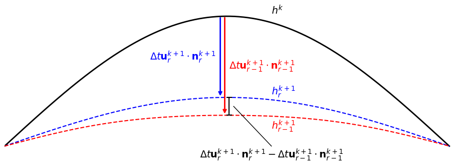
Figure 2 Illustration of the displacement estimate that is the basis of the stabilization method used for implicit iterations. The arrows mark the displacement from h^k to h^k+1 in two different implicit iterations. The vertical bar measures the difference between the two arrows, which is the displacement between two implicit iterations.

The main goal of this paper is to stabilize the implicit iterations using two slightly different FSSA terms subtracted from each other. At the first non-linear iteration, r=0, of each time step, an explicit FSSA-stabilized method is used just as for the purely explicit solver of Sect. 3. This renders a first guess that is close enough to the true implicit solution for the iterations to converge, this is the line labeled FSSA in Fig. 4b. For large time steps, the subsequent iterations must also be stabilized to avoid the growth of spurious oscillations, but applying the FSSA again would be erroneous since FSSA predicts the surface position at the next time step, not the next iteration. To create an appropriate stabilization term, we observe that the surface at implicit iteration r+1, i.e. $h_{r+\mathrm{1}}^{k+\mathrm{1}}$, is computed as

$$\begin{array}{}\text{(16)}& \begin{array}{rl}& {\left(h_{r+\mathrm{1}}^{k+\mathrm{1}},q\right)}_{\mathit{\omega }}={\left(h^k,q\right)}_{\mathit{\omega }}+\mathrm{\Delta }t\left(\left(-u_{x,r}^{k+\mathrm{1}}{\displaystyle \frac{\partial h_r^{k+\mathrm{1}}}{\partial x}}-u_{y,r}^{k+\mathrm{1}}{\displaystyle \frac{\partial h_r^{k+\mathrm{1}}}{\partial y}}\right.\right.\\ & {\left.\left.+u_{z,r}^{k+\mathrm{1}}\right),q\right)}_{\mathit{\omega }}={\left(h^k,q\right)}_{\mathit{\omega }}+\mathrm{\Delta }t\underset{{\mathrm{\Gamma }}_{\mathrm{s},r}^k}{\int }{\mathit{u}}_r^{k+\mathrm{1}}\cdot {\mathit{n}}_r^{k+\mathrm{1}}q\mathrm{d}{s}_r^{k+\mathrm{1}},\end{array}\end{array}$$

while the surface at the previous implicit iteration, $h_r^{k+\mathrm{1}}$, is computed as

$$\begin{array}{}\text{(17)}& \begin{array}{rl}& {\left(h_r^{k+\mathrm{1}},q\right)}_{\mathit{\omega }}={\left(h^k,q\right)}_{\mathit{\omega }}+\mathrm{\Delta }t\left(\left(-u_{x,r-\mathrm{1}}^{k+\mathrm{1}}{\displaystyle \frac{\partial h_{r-\mathrm{1}}^{k+\mathrm{1}}}{\partial x}}-u_{y,r-\mathrm{1}}^{k+\mathrm{1}}{\displaystyle \frac{\partial h_{r-\mathrm{1}}^{k+\mathrm{1}}}{\partial y}}\right.\right.\\ & {\left.\left.+u_{z,r-\mathrm{1}}^{k+\mathrm{1}}\right),q\right)}_{\mathit{\omega }}={\left(h^k,q\right)}_{\mathit{\omega }}+\mathrm{\Delta }t\underset{{\mathrm{\Gamma }}_{\mathrm{s},r-\mathrm{1}}^k}{\int }{\mathit{u}}_{r-\mathrm{1}}^{k+\mathrm{1}}\cdot {\mathit{n}}_{r-\mathrm{1}}^{k+\mathrm{1}}q\mathrm{d}{s}_{r-\mathrm{1}}^{k+\mathrm{1}}.\end{array}\end{array}$$

Therefore, the difference between two subsequent surfaces in the implicit iterations is

$$\begin{array}{}\text{(18)}& \begin{array}{rl}\left(h_{r+\mathrm{1}}^{k+\mathrm{1}},q\right)& -\left(h_r^{k+\mathrm{1}},q\right)=\mathrm{\Delta }t\left(\underset{{\mathrm{\Gamma }}_r^k}{\int }{\mathit{u}}_r^{k+\mathrm{1}}\cdot {\mathit{n}}_r^{k+\mathrm{1}}q\mathrm{d}{s}_r^{k+\mathrm{1}}\right.\\ & \left.-\underset{{\mathrm{\Gamma }}_{r-\mathrm{1}}^k}{\int }{\mathit{u}}_{r-\mathrm{1}}^{k+\mathrm{1}}\cdot {\mathit{n}}_{r-\mathrm{1}}^{k+\mathrm{1}}q\mathrm{d}{s}_{r-\mathrm{1}}^{k+\mathrm{1}}\right),\end{array}\end{array}$$

see Fig. 2 for a conceptual illustration. Recalling the similarity between the terms of the right-hand side of Eq. (13) and the expression above, we claim that the FSSA term must be augmented to be consistent with Eq. (18). The FSSA term of the previous iterations is thus subtracted from the FSSA term on the current iteration, leading to:

$$\begin{array}{}\text{(19)}& \begin{array}{rl}{\mathit{\theta }}_{\mathrm{1}}\mathrm{\Delta }t\underset{{\mathrm{\Gamma }}_r^k}{\int }\mathit{\rho }\mathit{g}& \cdot \mathit{v}{\mathit{u}}_r^{k+\mathrm{1}}\cdot {\mathit{n}}_r^{k+\mathrm{1}}\mathrm{d}{s}_r^{k+\mathrm{1}}\\ & -{\mathit{\theta }}_{\mathrm{2}}\mathrm{\Delta }t\underset{{\mathrm{\Gamma }}_{r-\mathrm{1}}^k}{\int }\mathit{\rho }\mathit{g}\cdot \mathit{v}{\mathit{u}}_{r-\mathrm{1}}^{k+\mathrm{1}}\cdot {\mathit{n}}_{r-\mathrm{1}}^{k+\mathrm{1}}\mathrm{d}{s}_{r-\mathrm{1}}^{k+\mathrm{1}}.\end{array}\end{array}$$

Here, we have introduced the parameters θ₁ and θ₂ for later convenience. We will call this method the subtraction-FSSA, and we will use Eq. (19) to stabilize the fully implicit discretization for r>0. By the subtraction-FSSA, the term Δtu⋅n in Eq. (15), which is the net distance traveled by the surface from one time step to another, is replaced by Eq. (18) to ensure that the correct surface displacement is used in the Reynolds transport theorem. Setting θ₁=1, θ₂=0 results in the original FSSA term and, for the new subtraction-FSSA, ${\mathit{\theta }}_{\mathrm{1}}={\mathit{\theta }}_{\mathrm{2}}=\mathrm{1}$. Exactly like for the original FSSA, the subtraction-FSSA of Eq. (19) is added to the Stokes equations. A key observation is that, if the iteration converges

$$\begin{array}{}\text{(20)}& \left(h_{r+\mathrm{1}}^{k+\mathrm{1}},q\right)-\left(h_r^{k+\mathrm{1}},q\right)\to \mathrm{0}\mathrm{as}r\to \mathrm{\infty },\end{array}$$

i.e. as the implicit discretizations converge, the difference between the surfaces at consecutive iterations tend to zero and thereby the stabilization also approaches zero. The iterations should therefore converge to the unstabilized implicit solution.

In some software programs, like Elmer/Ice, it is difficult to access the mesh and normal vector from iteration k, required in Eq. (19). For this purpose we introduce a simplified subtraction-FSSA, which only requires the velocity to be accessible from the previous iteration

$$\begin{array}{}\text{(21)}& \begin{array}{rl}{\mathit{\theta }}_{\mathrm{1}}\mathrm{\Delta }t\underset{{\mathrm{\Gamma }}_r^k}{\int }\mathit{\rho }\mathit{g}& \cdot \mathit{v}{\mathit{u}}_r^{k+\mathrm{1}}\cdot {\mathit{n}}_r^{k+\mathrm{1}}\mathrm{d}{s}_r^{k+\mathrm{1}}\\ & -{\mathit{\theta }}_{\mathrm{2}}\mathrm{\Delta }t\underset{{\mathrm{\Gamma }}_r^k}{\int }\mathit{\rho }\mathit{g}\cdot \mathit{v}{\mathit{u}}_{r-\mathrm{1}}^{k+\mathrm{1}}\cdot {\mathit{n}}_r^{k+\mathrm{1}}\mathrm{d}{s}_r^{k+\mathrm{1}}.\end{array}\end{array}$$

5 A second order implicit time-stepping scheme

For first order Euler discretizations of the free surface equation, the numerical error increases linearly with the time step. The increased stability of FSSA and fully implicit solutions allows for large time steps, which can introduce large errors. To reduce errors, we now construct higher order time-stepping schemes. It is of course trivial to exchange the discretization of the free surface equation with a higher-order scheme. However, the FSSA stabilization term was derived from a first-order discretization of the Reynold's transport theorem, and higher-order effects of the h-dependency of terms other than the body force term were ignored. The FSSA-stabilization will thus reduce the overall accuracy to first order. However, with the new implicit scheme introduced in Sect. 4 it is possible to achieve higher-order accuracy since the stabilization term of Eq. (19) tends to zero. Thus, a standard implicit higher-order scheme can be applied to the free surface. Here, we choose a second-order Crank–Nicolson scheme as well as a second-order Backward Differentiation (BDF2) scheme. We present these schemes on strong form and drop the index r for brevity of presentation. The Crank–Nicolson scheme is

$$\begin{array}{}\text{(22)}& \begin{array}{rl}{h}^{k+\mathrm{1}}& =h^k+\mathrm{\Delta }t\left({\displaystyle \frac{\mathrm{1}}{\mathrm{2}}}\left(-u_x^k{\displaystyle \frac{\partial h^k}{\partial x}}-u_y^k{\displaystyle \frac{\partial h^k}{\partial y}}+u_z^k\right)\right.\\ & \left.+{\displaystyle \frac{\mathrm{1}}{\mathrm{2}}}\left(-u_x^{k+\mathrm{1}}{\displaystyle \frac{\partial h^{k+\mathrm{1}}}{\partial x}}-u_y^{k+\mathrm{1}}{\displaystyle \frac{\partial h^{k+\mathrm{1}}}{\partial y}}+u_z^{k+\mathrm{1}}\right)\right)\end{array}\end{array}$$

where u^k+1 is the solution retrieved from the implicit iterations and u^k is the solution of the previous time step. The BDF2-scheme is

$$\begin{array}{}\text{(23)}& \begin{array}{rl}{\displaystyle \frac{\mathrm{3}{h}^{k+\mathrm{1}}-\mathrm{4}{h}^k+h^{k-\mathrm{1}}}{\mathrm{2}\mathrm{\Delta }t}}& =-u_x^{k+\mathrm{1}}{\displaystyle \frac{\partial h^{k+\mathrm{1}}}{\partial x}}-u_y^{k+\mathrm{1}}{\displaystyle \frac{\partial h^{k+\mathrm{1}}}{\partial y}}\\ & +u_z^{k+\mathrm{1}}.\end{array}\end{array}$$

6 Idealized numerical experiments

6.1 Overview

To evaluate the error, the convergence order and the efficiency of the subtraction-FSSA in its full and simplified form, we run the same idealized experiments as in Löfgren et al. (2022). The setup is relevant to mantle convection, and the experiments are inspired by the mantle convection experiments of, e.g. Rose et al. (2017) and Andrés-Martínez et al. (2015). The software used is Biceps (Löfgren, 2025b), which is a C$++$ finite element library developed specifically to solve two-dimensional Stokes-coupled free-surface problems. It relies on the Eigen3 library (Guennebaud and Jacob, 2010) for storing and solving linear systems. Biceps includes its own suite of finite element utilities, providing users with fine-grained control over the assembly process.

6.2 Experimental setup

The simulation domain consists of a two-dimensional horizontal slab of ice with an undulating upper surface, defined over the interval $x\in \mathit{\omega }=[\mathrm{0},L]$ m, where the length of the domain L is 100 km, see Fig. 3. The mean ice thickness is set to H=1.0 km, and the surface elevation varies sinusoidally with amplitude z₀=0.1 km.

$$z_{\mathrm{s}}\left(x\right)=H+z_{\mathrm{0}}\cos \left({\displaystyle \frac{\mathit{\pi }x}{L}}\right).$$

The ice is treated as a Newtonian fluid (𝔭=2, ε=0) with ν₀=10¹² Pa s⁻¹. Gravity is acting in the vertical direction with magnitude g=9.8 m s⁻², and the ice density is set to ρ=910 kg m⁻³. The surface is a material surface, i.e. a_s=0.

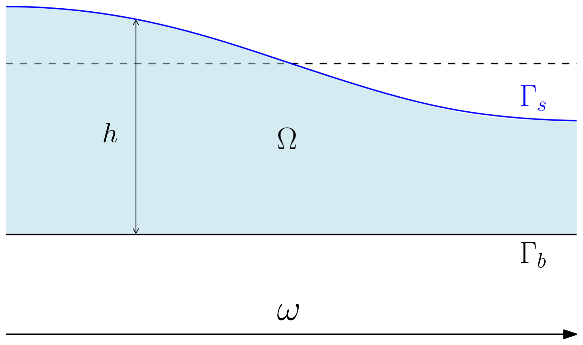
Figure 3 Experimental setup. Outlined is the bulk domain Ω, the free-surface domain ω, the surface Γ_s, the height of the surface h, and the bedrock Γ_b. The surface will relax to the equilibrium configuration (black dashed line) as time progresses.

The computational mesh is structured and consists of 50 elements in the horizontal direction and 5 elements in the vertical. In Löfgren et al. (2022, 2024) the mesh dependence of the stability properties was studied in detail. Triangular elements are used with a polynomial degree of 2 for velocity, 1 for pressure, and 1 for surface height. The time integration spans a final simulation time of T=20.0 years, which allows the surface to evolve significantly, yet remains far enough away from the steady-state configuration.

We perform experiments with first-order Euler schemes, Crank–Nicolson and BDF2, with and without stabilization, and with the maximum number of implicit iterations r_max being 1 (no implicitness), 2 (minimum implicitness) and 100 (allowing full implicitness). The convergence tolerance for the implicit iterations is set to $\mathrm{1}\times {\mathrm{10}}^{-\mathrm{9}}$ unless otherwise stated. Experiments are performed with time step sizes of Δt=0.001, 0.005, 0.01, 0.05, 0.1, 0.5, 1, 2.5, 5, 10, and 20 years. For each experiment, we measure the error and count the number of iterations, i.e. Stokes solves.

To measure the errors, we construct a reference solution by running a second-order Adams–Bashforth time-stepping scheme

$$\begin{array}{}\text{(24)}& \begin{array}{rl}{h}^{k+\mathrm{1}}& =h^k+{\displaystyle \frac{\mathrm{\Delta }t}{\mathrm{2}}}\left(\mathrm{3}\left(-u_x^k{\displaystyle \frac{\partial h^k}{\partial x}}+u_z^k\right)\right.\\ & \left.-\left(-u_x^{k-\mathrm{1}}{\displaystyle \frac{\partial h^{k-\mathrm{1}}}{\partial x}}+u_z^{k-\mathrm{1}}\right)\right)\end{array}\end{array}$$

for a very small time step of Δt=0.00001 without FSSA-stabilization. Note that Adams–Bashforth is an explicit method, which is unstable for large time steps but stable for Δt=0.00001. The convergence of the surface elevation is monitored using a normalized L₂-like metric:

$$\Vert \mathrm{\Delta }h\Vert =\sqrt{{\displaystyle \frac{\mathrm{1}}{n}}\sum _{i=\mathrm{1}}^n{\displaystyle \frac{{\left(h_r^{k+\mathrm{1},i}-h_{r+\mathrm{1}}^{k+\mathrm{1},i}\right)}^{\mathrm{2}}}{{\left(h_r^{k+\mathrm{1},i}-H\right)}^{\mathrm{2}}}}},$$

where $h_r^{k+\mathrm{1}}$ and $h_{r+\mathrm{1}}^{k+\mathrm{1}}$ denote the surface height at two consecutive implicit iterations and i is the surface mesh node.

6.3 Results

6.3.1 First order schemes

The results are shown in Figs. 4 and 5, where errors in surface position are plotted against time-step size. The largest time step for which even the unstabilized explicit Euler scheme is stable is Δt=0.01 years, see Fig. 5a. The unstabilized implicit solver (i.e. the backward Euler or BDF1 solver) is also only stable for time steps up to Δt=0.01 years; see Fig. 5c. For Δt=0.01, one can see that the surface of the FSSA-stabilized “explicit” Euler discretization lies between the unstabilized and the fully implicit BDF1 method Fig. 4a. This is expected since FSSA only modifies the integration domain of the right-hand side of the Stokes equations, while the left-hand-side integration domains are still treated explicitly, so the discretization is a hybrid between explicit and implicit approaches. However, the FSSA-stabilized solution is close to the implicit solution, perhaps indicating that since the flow is gravity driven, the implicit treatment of the left-hand side is not as important as that of the right-hand side.

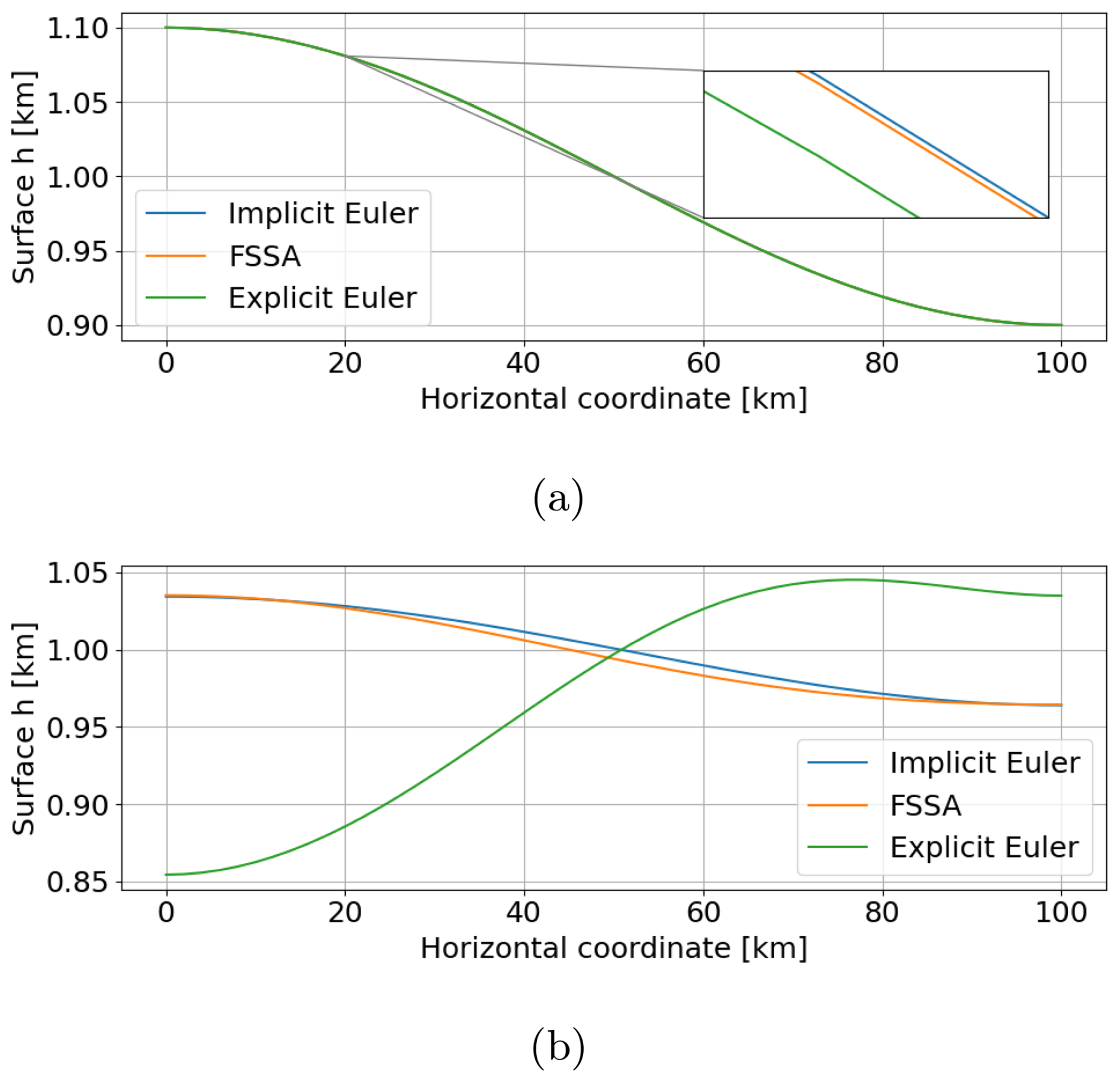
Figure 4 Explicit Euler with (orange) and without FSSA (green), as well as the implicit solution (blue). The top panel (a) shows the solutions for a single small time-step of size Δt=0.01 years, for which all methods are stable. The inserted box is a zoom in around x=20, y=1.0808. The bottom panel (b) shows the solutions after one single large time step of size Δt=20 years for which the unstabilized Explicit Euler solution is unstable.

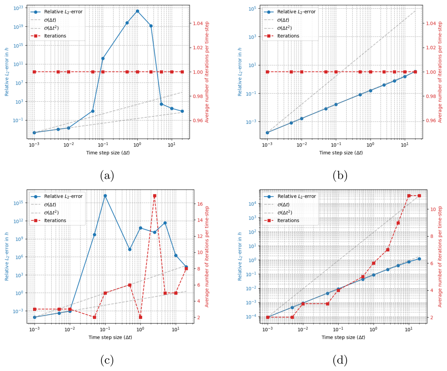
Figure 5 Error in surface position h (in km) as computed with first order schemes for different time-steps Δt (in years). The results in panel (a) are computed using Forward Euler for the free surface, and no FSSA. The very large errors for intermediate time-step sizes are due to high frequency oscillations. For the three largest time steps, the solution is smooth but erroneous. The results of in panel (b) are computed using Forward Euler, with FSSA (θ₁=1, θ₂=1). The results in panel (c) are computed using the fully implicit solver, without FSSA while the results of panel (d) are computed using the fully implicit solver with the subtraction-FSSA. For the implicit solver, a maximum of 100 implicit iterations is permitted per time step and the convergence tolerance $\mathrm{1}\times {\mathrm{10}}^{-\mathrm{9}}$ was. The reference solution is computed with Δt=0.00001 years and the final time is 20 years.

In Fig. 4b, all three solutions are shown for a large time step of Δt=20. The unstabilized explicit Euler scheme is unstable, and the instability is a low-frequency sloshing or ”drunken sailor” type of instability similar to those of e.g. Kaus et al. (2010). The FSSA-stabilized solution and the implicit solution stabilized by Eq. (19) are stable and close to each other, differing mostly at the inflection point. Interestingly, the overall error as shown in Fig. 5 is not lower for the fully implicit solver, indicating that the FSSA error is lower than the overall discretization error for first-order schemes.

Note that the behavior of the implicit solver depends on the convergence tolerance. If the convergence tolerance is lower than the overall discretization error, it will use up unnecessarily many iterations, and high-frequency errors will eventually start to grow. These high frequency oscillations can be mitigated by, for example, an artificial viscosity approach on the free surface equation, but we instead choose to terminate the iterative solver if $\Vert \mathrm{\Delta }h\Vert$ grows, as this is more efficient. Note also that even though the FSSA solution from the first iteration is close to the converged implicit solution, it is not possible to only use FSSA in the first time-step, i.e. θ₁=1 is necessary for all iterations.

6.3.2 Second order schemes

The results are shown in Figs. 6 and 7. Just like the the first-order Euler method, the simulations are unstable without the stabilization. Simply adding the FSSA stabilization renders first-order convergence, while our idea of subtracting two FSSA terms from different iterations according to Eq. (19) renders second-order convergence for both Crank–Nicolson and BDF2. An interesting result of this is that only two iterations (Stokes solves) are needed in each time step to achieve second-order convergence. This is very advantageous for efficiency. For example, if a user requires an accuracy of 10⁻⁴, a time step $\mathrm{\Delta }t={\mathrm{10}}^{-\mathrm{3}}$ is needed for the first-order method, that is, $\mathrm{20}/{\mathrm{10}}^{-\mathrm{3}}=\mathrm{20}\mathrm{000}$ time steps are needed. The most efficient first-order method is to choose one implicit iteration, i.e., without implicitness, only FSSA stabilization. Then one Stokes solve is needed per time-step, which results in 20 000 Stokes solves. For Crank–Nicolson and BDF2, this accuracy is reached for Δt=0.1, i.e., $\mathrm{20}/\mathrm{0.1}=\mathrm{200}$ time steps are needed. With two Stokes solves per time step, this means that 400 Stokes solves are needed in total. The speedup should thus be about $\mathrm{20000}/\mathrm{400}=\mathrm{50}$, which is remarkable.

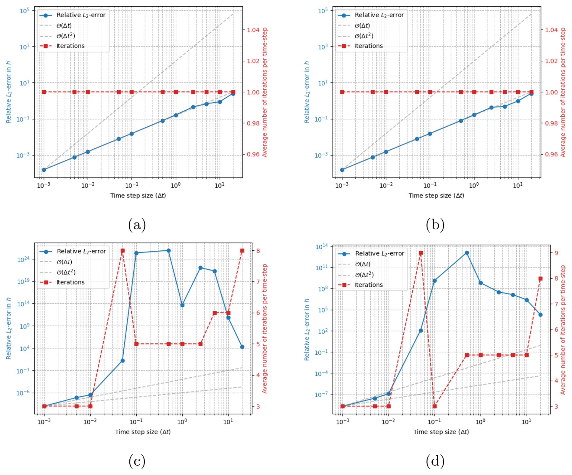
Figure 6 Error in surface position h (in km) as computed with non-working “second order” schemes for different time-steps Δt (in years). Panel (a) and (b) shows results computed with Crank–Nicolson and BDF2 respectively, without implicit iterations, and FSSA is instead used to approximate uⁿ⁺¹. Panel (c) and (d) shows results computed with Crank–Nicolson and BDF2 respectively, with implicit iterations but without stabilization. In panel (a) and (b) first order accuracy is seen, while second order accuracy is seen in panel (c) and (d) but only for very small time-steps. The reference solution is computed with Δt=0.00001 years and the final time is 20 years.

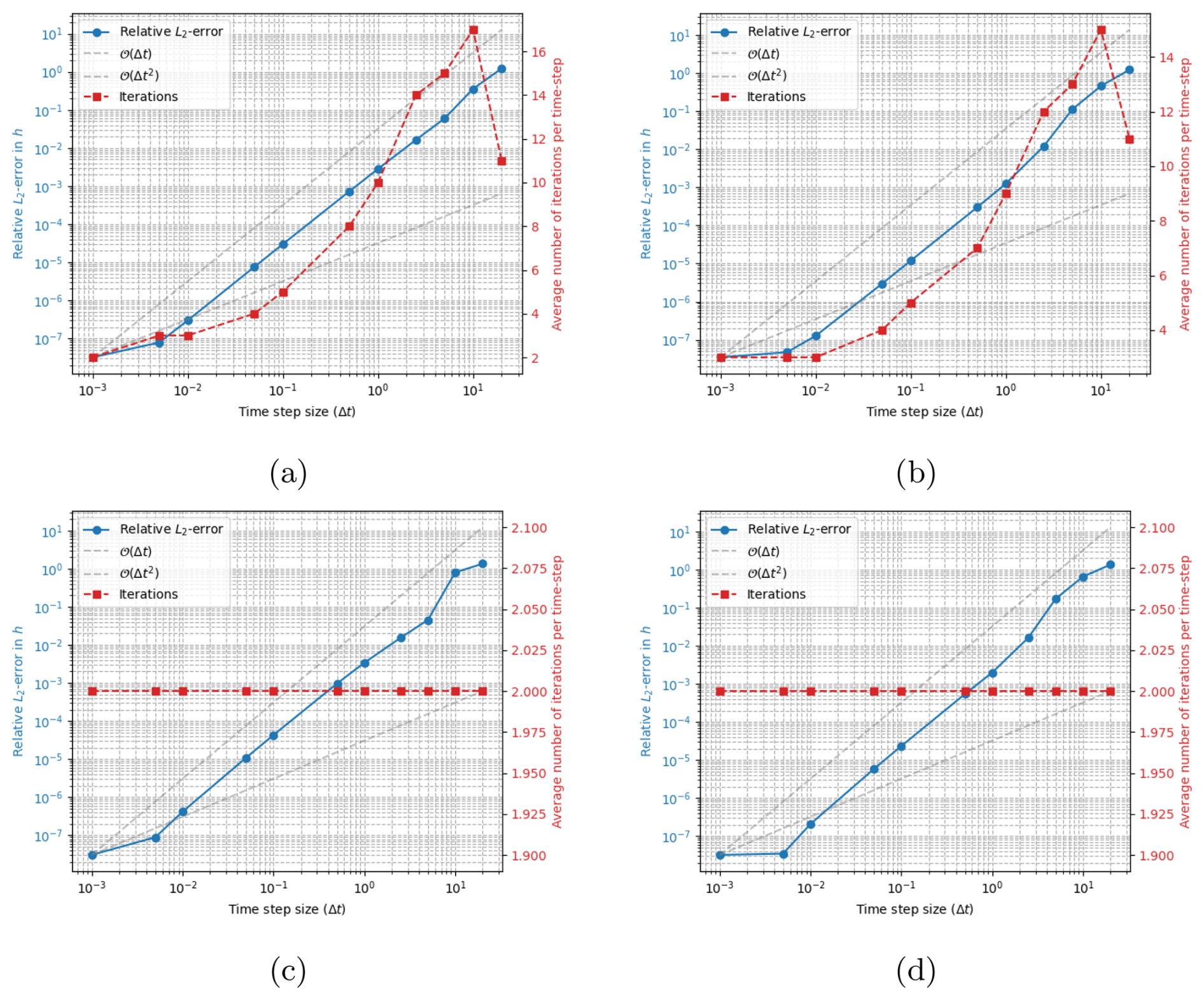
Figure 7 Error in surface position h (in km) as computed with working second order schemes for different time-steps Δt (in years). All results are computed using the fully implicit solver stabilized with the subtraction-FSSA. Panel (a) and (b) shows results computed with Crank–Nicolson and BDF2 respectively, permitting a maximum of 100 implicit iterations per time step and with a convergence tolerance of $\mathrm{1}\times {\mathrm{10}}^{-\mathrm{9}}$. Panel (c) and (d) shows results computed with Crank–Nicolson and BDF2 respectively but only permitting a maximum of 2 implicit iterations and keeping the convergence tolerance at $\mathrm{1}\times {\mathrm{10}}^{-\mathrm{9}}$. The reference solution is computed with Δt=0.00001 years and the final time is 20 years.

6.3.3 The simplified subtraction-FSSA

The simplified scheme of Eq. (21) performs as well as the exact method of Eq. (19) for both first order and second order schemes, see Fig. 8. Just as with the full subtraction FSSA, achieving second-order convergence requires only two coupled iterations. as for the full subtraction-FSSA, only two coupled iterations are needed to obtain second order convergence.

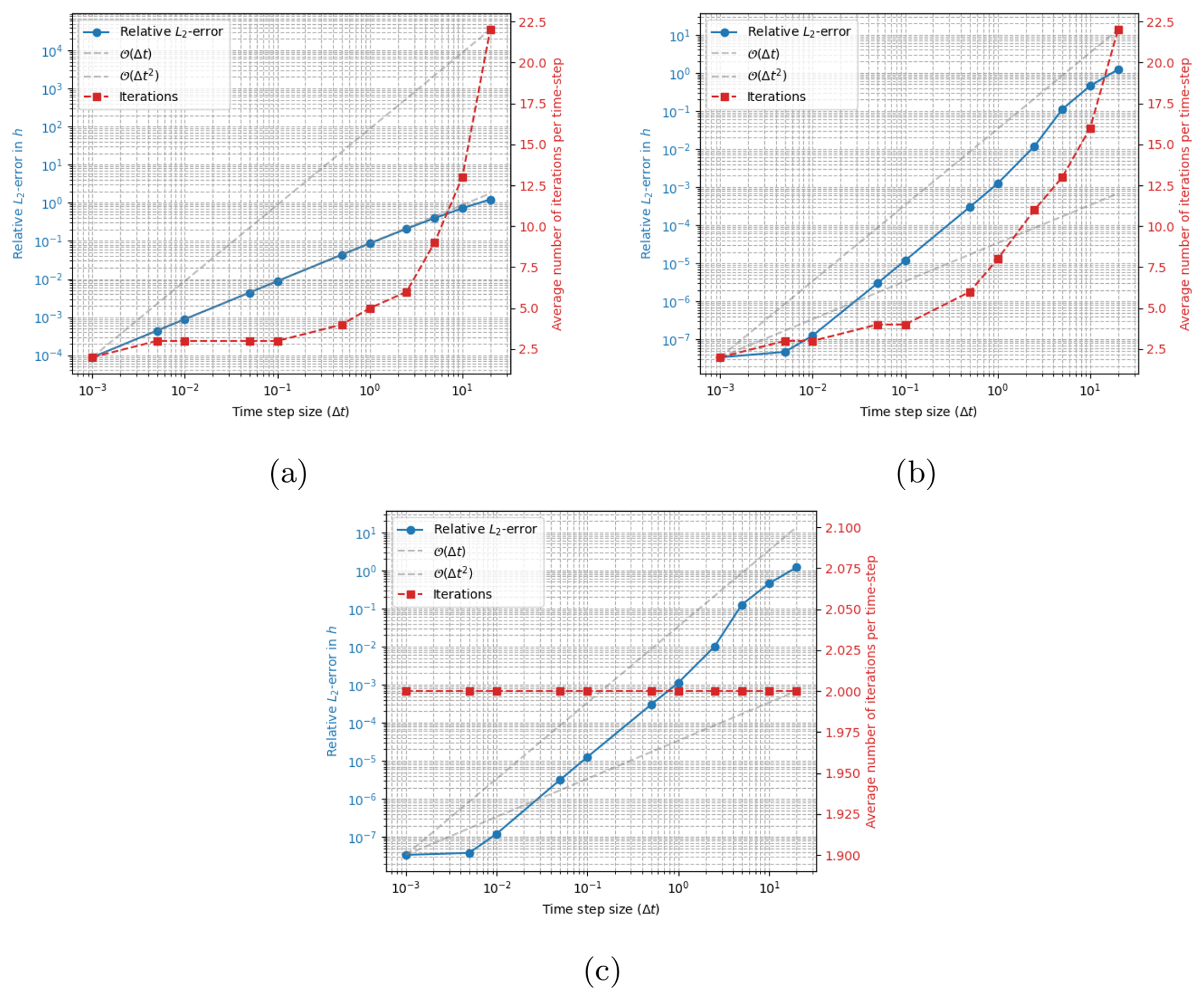
Figure 8 Results computed using a fully implicit solver stabilzed by the simplified stabilization method of Eq. (21). Panel (a) and (b) shows results computed with BDF1 and BDF2 respectively, permitting a maximum of 100 implicit iterations per time-step. The results of panel (c) are computed using BDF2 but only permitting a maximum of 2 implicit iterations per time-step. The convergence tolerance is $\mathrm{1}\times {\mathrm{10}}^{-\mathrm{9}}$ in all simulations. As with the exact stabilization of Eq. (19), 2 coupled iterations are enough to reach second order convergence. The reference solution is computed with Δt=0.00001 and the final time is 20 years.

7 Application to glacier simulations

7.1 Overview

An important application of the methods in this paper is in the simulation of glaciers and ice sheets. These types of simulations exhibit two key characteristics which the idealized mantle convection setup of the previous section does not:

• Non-linear rheology, with $\mathfrak{p}=\mathrm{4}/\mathrm{3}$ in Eq. (4).

• A constraint on the free surface, h, ensuring that the surface stays above the bedrock.

The non-linear rheology means that each Stokes solve is more expensive due to internal Picard fixed-point iterations that resolve the nonlinear viscosity. Reducing the number of time-steps would therefore be even more beneficial. The constraint on the free surface is implemented in such a way that it can impact the number of implicit iterations and possibly the accuracy of the methods, which is investigated in the experiments.

We evaluate the accuracy and efficiency of glacier simulations using the popular ice sheet simulation code Elmer/Ice (Gagliardini et al., 2013). Since accessing the mesh at a previous iteration in Elmer/Ice is nontrivial, we implement the simplified version of the stabilization method as in Eq. (18). It should be noted that without stabilization, the free surface of glaciers and ice sheets is prone to instabilities, and therefore relaxation of this solution is routinely used in Elmer/ice, which might be unnecessary in simulations with FSSA.

We choose to model a so-called Perlin glacier similar to that of Löfgren et al. (2024), a setup that allows for relatively fast simulations and thus thorough experimentation with parameter choices. Note that this type of mountain glacier is more stable than an ice sheet (compare the results of Löfgren et al., 2024 to Löfgren et al., 2022), but that it has the important feature of a moving glacier front, which activates the constraint on the surface h. In the following section, we outline the strategy used in Elmer/Ice to handle the constraint as described in Durand et al. (2009) and Gagliardini et al. (2013).

7.2 The free surface constraint

To prevent the ice surface from falling below the bedrock elevation b, a constraint is imposed on the free surface:

$$\begin{array}{}\text{(25)}& h(x,t)-H_{\min }\ge b(x,t),\end{array}$$

where H_min>0 avoids remeshing near the glacier front.

Discretizing the free surface equation (Eq. 10) results in the linear system

$$\begin{array}{}\text{(26)}& \mathbf{A}\mathit{h}=\mathit{f},\end{array}$$

with A s the finite element matrix, h the surface elevation vector, and f the forcing vector that includes the vertical velocity and surface mass balance. The nodes on the surface boundary Γ_s are labeled as inactive if they satisfy the constraint and active if they do not. The system is solved iteratively: First, the discretized free-surface equation (Eq. 26) is solved. Each node is then classified as either active or inactive. A previously inactive node that violates the constraint is reclassified as active. To determine whether a previously active node should become inactive, the residual r_j is evaluated: if r_j<0, the node is reclassified as inactive; if r_j>0, it remains active. For active nodes, a Dirichlet condition is enforced by modifying the system such that $A_{ij}^{\prime }={\mathit{\delta }}_{ij}$ and $f_i=H_{\min }+b$, setting the surface to the minimum allowable thickness, which may increase the residual in those nodes. The system (Eq. 26) is then solved again, which requires a new check for active and inactive nodes. This iterative process continues until the solution h converges. The full details of this procedure are described in Sect. 3.5 in Durand et al. (2009) and Sect. 6.5 in Gagliardini et al. (2013).

Note that the standard approach in glaciology is to not use implicit iterations. This does not allow the velocity to update in the system (Eq. 26) within one time step, which for large time steps could affect behavior close to the areas where the constraint is active, i.e., close to the glacier front.

7.3 Experimental setup

The Perlin glacier is a synthetic two-dimensional glacier flowing down a mountainside (Fig. 9). The bedrock elevation is constructed using so-called Perlin noise (Perlin, 1985) and takes the form

$$\begin{array}{}\text{(27)}& \begin{array}{rl}b\left(x\right)& ={\displaystyle \frac{\mathit{\alpha }}{L_x}}{\left(x-L_x\right)}^{\mathrm{2}}+C^{\mathrm{1}}{\mathrm{octave}}_{\mathrm{1}}\left(x\right)+C^{\mathrm{2}}{\mathrm{octave}}_{\mathrm{2}}\left(x\right)\\ & +C^{\mathrm{3}}{\mathrm{octave}}_{\mathrm{3}}\left(x\right),\end{array}\end{array}$$

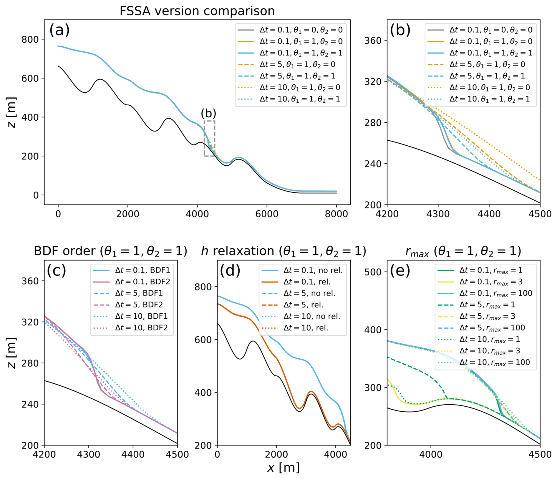
Figure 9 The surface elevation, h, of the Perlin glacier after a 400-year simulation, with varying parameters. Panels (a) and (b) show the surface elevation computed with BDF1 across the time step sizes 0.1, 5 and 10 years with subtraction-FSSA and the original FSSA formulation, along with the reference simulation with no FSSA stabilization. Panel (c) shows a comparison between BDF order 1 and 2 across simulations with time step sizes of 0.1, 5 and 10 years, all of which include the subtraction-FSSA. Panel (d) shows simulations with time step sizes of 0.1, 5 and 10 years with and without relaxation of the free-surface solver. Lastly, panel (e) shows the surface elevation with and without coupled iterations for time step sizes of 0.1, 5 and 10 years. Across all figures, the black line indicates the bed elevation.

where L_x=8000 m is the horizontal extent of the domain and α=0.1 controls the mean slope of the bedrock. The octaves, octave_i(x), represent noise of various frequencies, and are piecewise cubic splines where the nodes of the interpolation have an equidistant spacing of $\mathrm{2000}/{\mathrm{2}}^{i-\mathrm{1}}$ and the gradients at the nodes are randomly generated, see Appendix A in Löfgren et al. (2024). The approach results in a topography that resembles natural bedrock (Löfgren et al., 2024). The topography chosen corresponds to the α=0.1 simulation in Löfgren et al. (2024).

At the initial time t=0, the glacier domain contains an artificial ice layer of thickness 10 m, corresponding to the minimum allowed ice thickness H_min. The glacier is then built up by surface accumulation, prescribed at the rate

$$\begin{array}{}\text{(28)}& a_{\mathrm{s}}=\max \left(\mathrm{1}-{\displaystyle \frac{\mathrm{3}x}{L_x}},\mathrm{0}\right).\end{array}$$

During the simulation, the glaciated area is defined as the region where the ice thickness exceeds H_min. Areas with thickness equal to or less than H_min are considered ice-free, consistent with standard Elmer/Ice procedures. Simulations are run until 400 years.

The viscosity is defined by $\mathfrak{p}=\mathrm{1}/n+\mathrm{1}$, ${\mathit{\nu }}_{\mathrm{0}}=\mathrm{1}/{\mathrm{2}}^{(\mathrm{1}/n+\mathrm{1})}/\mathrm{2}{A}^{\mathrm{1}/n}$, $\mathit{\epsilon }=\mathrm{2}\times {\mathrm{10}}^{-\mathrm{10}}$, where the Glen exponent n=3 and the ice fluidity factor A=100 yr⁻¹ MPa⁻³, that is, the ice is very viscous and shear-thinning. The density of ice is 910 kg m⁻³ and the acceleration of gravity is −9.8 m s⁻². At the bottom Γ_b we use a linear Weertman sliding law (Eq. 8) with friction coefficient C=0.1 MPa m⁻¹ a, which differs from the friction law used in Löfgren et al. (2024), but results in a similar ice geometry.

Triangular elements are used with a polynomial degree of 1 for velocity, 1 for pressure, and 1 for surface height. To circumvent the inf-sup condition, we employ the stabilization method of Franca and Frey (1992), a common choice in Elmer/Ice. The mesh is structured with 10 vertical layers and 1000 horizontal elements. During the simulation, the mesh deforms vertically to fit the evolving free surface, and the minimum thickness H_min prevents the elements from degenerating to zero thickness.

The nonlinear viscosity is resolved using Picard fixed-point iterations with a convergence tolerance of 10⁻⁸ and a relaxation factor of 2/3. The linearized system is solved at each nonlinear iteration with the MUMPS direct solver (Amestoy et al., 2001). The free surface equation is stabilized with streamline upwind Petrov-Galerkin stabilization (SUPG) (Gagliardini et al., 2013) and the resulting linear system is solved with the BiCGStab method, using a convergence tolerance of 10⁻⁹. The convergence tolerance for the implicit iterations is set to $\mathrm{1}\times {\mathrm{10}}^{-\mathrm{9}}$ as in the idealized experiments, but no divergence (growing $\Vert \mathrm{\Delta }h\Vert$) check is needed to terminate the iterations, probably due to the use of SUPG.

The experiments aim to study how the geometry of the glacier front and CPU time depend on

• the time step sizes $\mathrm{\Delta }t=\mathrm{0.1},\mathrm{5},\mathrm{10}$,

• the number of maximum allowed implicit iterations r_max=1, 3, 100,

• FSSA stabilization (θ₁=0, 1, θ₂=0, 1),

• the order of discretization of the free surface (1 or 2), and the relaxation of the free surface (0, 0.5).

The simulations with a time step of 0.1 are used to produce reference solutions. The time steps of 5 and 10 years are very large. The second-order free surface discretization of choice is BDF2, since this approach is common in Elmer/Ice and showed results, which performed as well as Crank–Nicolson in the idealized experiments.

7.4 Results

In Fig. 9 the glacier geometry is shown for all the simulations performed, while the efficiency is illustrated in Fig. 10. The stability limit for the unstabilized method lies between 1 and 5 years, which is why the case ${\mathit{\theta }}_{\mathrm{1}}={\mathit{\theta }}_{\mathrm{2}}=\mathrm{0}$ is not shown for $\mathrm{\Delta }t=\mathrm{5},\mathrm{10}$. The largest stable time-step of similar simulations was studied at length in Löfgren et al. (2024).

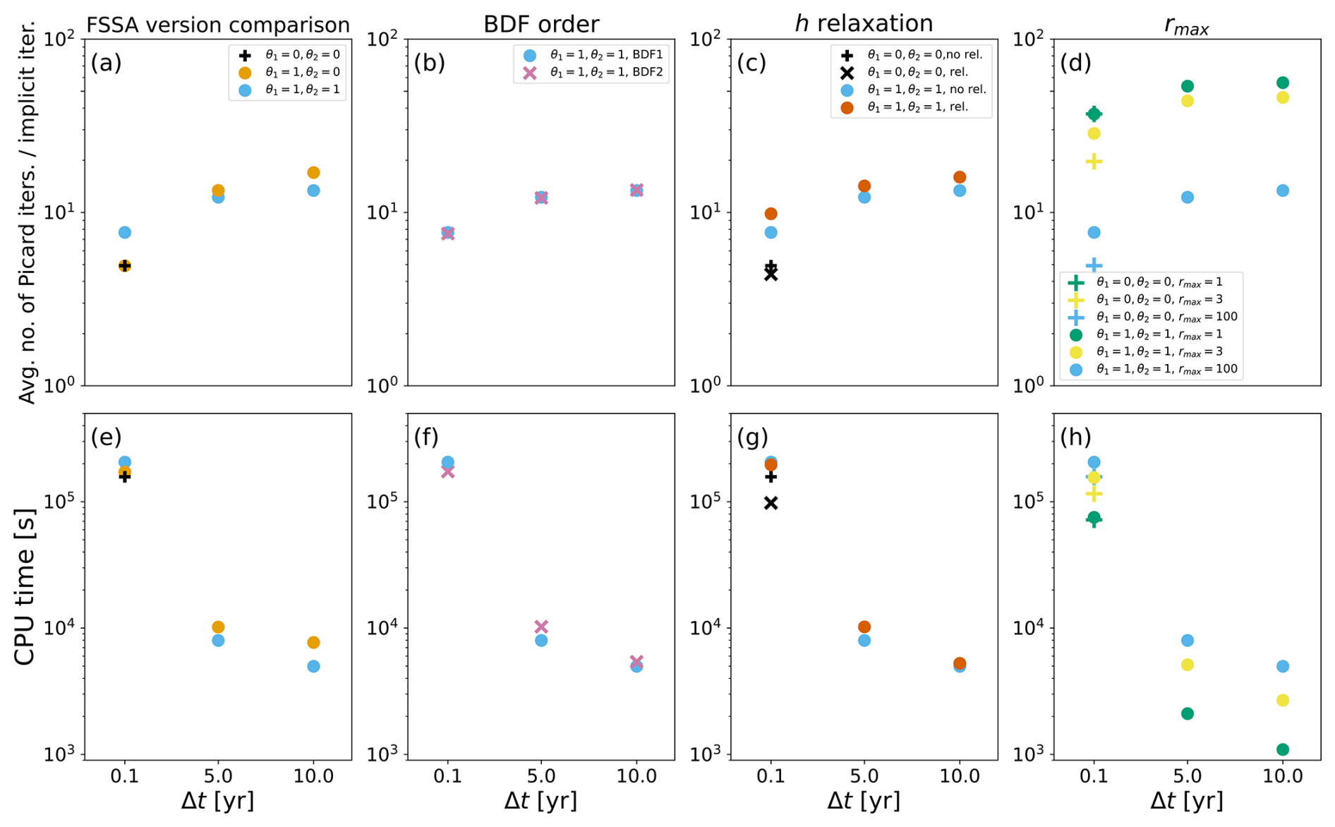
Figure 10 The top panels show the average number of Picard fixed point iterations per implicit iteration, and the bottom panels show the CPU time for the same simulations as in Fig. 9. Panels (a) and (e) illustrate the effect of the FSSA formulation (subtraction-FSSA, ${\mathit{\theta }}_{\mathrm{1}}={\mathit{\theta }}_{\mathrm{2}}=\mathrm{1}$, the original FSSA θ₁, θ₂=0 and no FSSA, ${\mathit{\theta }}_{\mathrm{1}}={\mathit{\theta }}_{\mathrm{2}}=\mathrm{0}$) across the time step sizes 0.1, 5 and 10 years. These simulations are performed with BDF1 and r_max=100, and with no surface relaxation. Panels (b) and (f) illustrate the effect of the BDF order in simulations with r_max=100, no surface relaxation and subtraction-FSSA stabilization applied. Panels (c) and (g) illustrate the effect of surface relaxation in simulations with BDF1, r_max=100, with and without subtraction-FSSA. Lastly, panels (d) and (h) show the effect of the maximum allowed implicit iterations r_max, in simulations with BDF1, r_max=100, with and without subtraction-FSSA.

Figure 9a and the zoomed in version of Fig. 9b show the glacier front for first-order Euler schemes with implicit iterations (i.e., BDF1). The maximum allowed implicit iterations is r_max=100 and no surface relaxation is used. It can be seen that the glacier front is in approximately the same position for the stabilized simulations (θ₁=1) with large time steps $\mathrm{\Delta }t=\mathrm{5},\mathrm{10}$ as it is for the reference solutions where Δt=0.1, although the shape is smoother. The front is more accurate for the new subtracted-FSSA method (θ₂=1) than it is for the original FSSA method (θ₂=0), and as expected, Δt=5 gives a better result than Δt=10. The CPU time is dominated by the number of linear Stokes solves, which is the number of Picard iterations per implicit iteration × number of implicit iterations × number of time steps. As expected, the number of nonlinear Picard iterations decreases somewhat for small time steps and with an increased number of implicit iterations (Fig. 10a). This expected since the initial guess to the Picard solver is better in these cases (the initial is the solution from the previous time step and implicit iteration). The decreased number of time steps still renders the large time-step simulations much more efficient, as can be seen in Fig. 10e.

Figure 9c shows the effect of using a higher-order BDF2 scheme instead of the first-order Euler (BDF1) scheme. BDF2 is more accurate than BDF1, and notably it is more accurate to run a time step of Δt=10 using BDF2 than a time-step of Δt=5 using BDF1. As can be seen in Fig. 10b and f, there is a very small computational cost associated with switching to BDF2. In Fig. 9d, the effect of switching on the free surface relaxation is illustrated. The accuracy is severely affected by doing so, while the efficiency is not impacted (see Fig. 10c and g).

Finally, Fig. 9e, the impact of restricting the number of implicit iterations r_max is shown. For r_max=1, i.e. without implicit iterations, the front is delayed for the large time steps. This is likely due to the fact that the iterations used to impose the constraint described in Sect. 7.2 benefit from the velocity updates that the implicit iterations offer. In the idealized experiments, we showed that r_max=2 is enough to yield accurate results. However, for the Perlin glacier, r_max=2 still yields a delayed front, while r_max=3 yields as accurate results as r_max=100. The extra iteration needed in the glacier experiments compared to idealized experiments is probably due to the constraint of the free surface. The computational cost is the highest for r_max=100 (Fig. 9h) but is not 100 times higher, as expected, since the number of coupled iterations is terminated by the convergence tolerance check rather than the maximum number of iterations, and since the number of Picard iterations per coupled iteration is lower for r_max=100 (Fig. 9d). Setting r_max=3 slightly reduces the computational cost, whilst retaining good accuracy.

8 Conclusion

We have developed a fully implicit method that allows for very large time-steps as well as second-order accuracy in simulations of viscous free-surface flow simulations. The method has important applications in e.g. ice sheet and glacier modelling and geodynamics. The implicitness allows for large time-steps and thereby simulation speedup, while second order schemes keep accuracy high. The key is a new stabilization scheme, the subtraction-FSSA, which extends the original FSSA approach of Kaus et al. (2010), Löfgren et al. (2022, 2024) and Henry et al. (2025). Compared to the original FSSA stabilization, our new scheme increases accuracy, not only because it enables second-order time-stepping schemes but also because it allows for a more accurate representation of the free-surface constraint preventing negative thickness at ice sheet and glacier margins. We further find that a simplified, easy-to-implement variant of the implicit iterations performs equally well as the full method and requires only access to the velocity of the previous iteration.

For first-order schemes, our implicit solver matches the accuracy of explicit FSSA in unconstrained geodynamic problems, confirming that FSSA already approximates an implicit solution well in such cases. In contrast, for moving glacier fronts, implicit iterations are substantially more accurate. It is overall more computationally efficient to use large time steps with three implicit iterations compared to using smaller time-steps with no implicit iterations.

Second-order schemes improve accuracy for both unconstrained and constrained (glacier) problems, requiring only two implicit iterations for the former and three for the latter, keeping computational costs low. The approach of using implicit iterations to construct higher order schemes appears especially appealing for glacier and ice sheet simulations, where the implicit iterations are needed regardless for resolving the minimum thickness constraint with large time-steps. Implementations such as BDF2 add minimal overhead, needing only a small modification to the left-hand side of the free-surface equation (Eq. 23). Overall, second-order implicit time-stepping with large time-steps is generally more efficient than first-order explicit schemes.

Future work will refine stopping criteria for implicit iterations and explore how to further increase accuracy near the glacier front, where a minimum thickness constraint is needed. None-the-less, subtraction-FSSA represents a major advance in accuracy and efficiency. Its integration into Elmer/Ice makes it readily available to the ice sheet community, paving the way for faster, more precise glacier and ice sheet simulations.