Towards an integrated inventory of anthropogenic emissions for China

Despite ongoing efforts to reduce pollution, persistent ozone pollution in China remains a public health concern. To better understand the causes of ozone pollution in China and to assess and evaluate the effectiveness of past, current, and planned targeted pollution control strategies, estimates of the amounts of pollutants emitted from various sources are needed. To this end, we have developed harmonized and integrated anthropogenic emission inventories for China, incorporating information from the existing national inventory for mainland China (MEIC) and three global inventories (CEDS, CAMS, HTAP) to cover areas outside of China. The newly developed China INtegrated Emission Inventory (CINEI) includes emissions in China from sectors currently omitted from the MEIC (ships, aviation, waste, and agriculture) that we incorporate from the global inventories. To ensure harmonized emissions data, we performed mapping between different inventories, a process used to achieve consistency between sectors, spatial resolution, and speciation of non-methane volatile organic compounds (NMVOCs). These harmonized and integrated inventories for China were used to drive WRF-Chem simulations for January (winter) and July 2017 (summer). Through a detailed evaluation of model results against available observations, we show that while the direct use of global inventories alone can lead to severe over- or underestimation of pollutant mixing ratios, CINEI inventories perform satisfactorily in simulating ozone (12 % in summer and 43 % in winter normalized mean bias) and its precursors, including nitrogen dioxide (NO₂, −0.5 % in summer and 40 % in winter) and carbon monoxide (CO, −50 % in both seasons). Based on the comparison and modeling of this study, valuable insights into the spatio-temporal variability of ozone and the subsequent design of future ozone mitigation strategies in China were provided.

1 Introduction

China's air quality has improved rapidly since 2013 in response to the implementation of mitigation strategies (Zhang et al., 2019). Concentrations of particulate matter (PM_2.5) and primary pollutants (e.g., nitrogen oxides, sulfur dioxide, and carbon monoxide) have decreased Wang et al., 2019; Liu and Wang, 2020; Wang et al., 2023. However, ground-level ozone pollution remains severe. In 2017, the population-weighted exposure-averaged mixing ratio of ozone in China reached 68.2 parts per billion by volume (ppbv) (Yin et al., 2020), exceeding the World Health Organization (WHO) air quality standard of 50 ppbv (Lyu et al., 2023; WHO, 2021). Ground-level ozone is a secondary pollutant formed in complex photochemical reaction chains from its precursors, including nitrogen oxides (NO_x = NO + NO₂), carbon monoxide (CO), and non-methane volatile organic compounds (NMVOCs). Therefore, the amounts of emitted precursors based on different anthropogenic emission inventories may lead to different estimates of ozone mixing ratios. To investigate near-surface ozone pollution, its multi-year changes, and the effects of sectoral emissions of precursors on ozone distribution over China, it is essential to accurately represent the amount and spatiotemporal variations of anthropogenic emissions of ozone precursors in emission inventories (Li et al., 2017; Chang et al., 2022; Smith et al., 2022; Monks et al., 2015). Therefore, emission inventories are essential to provide the information needed to formulate effective strategies to further improve air quality (Hoesly et al., 2018).

Over the past decade, anthropogenic emissions in China have undergone rapid changes due to air pollution reduction strategies (Fig. S1a in the Supplement). In particular, since 2013 during the implementation of 12th Five-Year Plan period (12th Five-Year Plan, 2011), there were significant reductions in anthropogenic emissions of −27 % for NO_x and −17 % for CO (Zheng et al., 2018). These reductions were due to measures such as setting ultra-low emission standards for vehicles and factories, improving air quality control technologies, and phasing out high-emitting factories (Li et al., 2017; Lu et al., 2020). After 2010, CO and NO₂ mixing ratios gradually fell below the WHO standards of 0.4 parts per million by volume (ppmv) for CO and 20 ppbv for NO₂ (Sect. S1 and Fig. S1b). Despite these significant improvements in air quality (Zhang et al., 2019), there is growing concern about unintended increases in ozone levels (Li et al., 2019; Lu et al., 2020), which may result from the co-effects of reduced NO_x emissions and increased NMVOC emissions (Li et al., 2019). As a result, specific strategies targeting NMVOC emissions were introduced in 2015, especially in the petrochemical and organic chemical industries. Despite these measures, maximum daily 8-h average ozone levels remained high in 2022 (Fig. S1b) and frequently exceeded the WHO thresholds during the warm season (April to October, Fig. S1b). Although total NMVOC emissions have decreased in China, some studies attribute the observed increase in ozone over the past decade to the increasing contribution of anthropogenic NMVOC emissions, especially aromatics, alkenes, and oxygenated VOCs (OVOCs), mainly from the petrochemical industry and solvent use, to the total NMVOCs (Li et al., 2014; Zhang et al., 2020, 2021; McDonald et al., 2018). In order to investigate the drivers of recent changes in ozone pollution in China, it is crucial to develop accurate emission inventories that reflect policy-driven changes in anthropogenic emissions.

However, existing anthropogenic emission inventories encounter discrepancies in sectoral emission (Solazzo et al., 2021). The discrepancy raises concerns about their accuracy and reliability (Crippa et al., 2021; McDonald et al., 2018). Anthropogenic emission inventories are typically constructed in a bottom-up manner, with sectoral emissions quantified using activity data and emission factors (Solazzo et al., 2021). Activity data are mainly derived from official statistics (see Sect. S2 for details). Emission factors provide the amount of emissions released per activity (Sect. S2). To obtain gridded emissions with specified NMVOC speciation and high spatiotemporal resolution, we need more detailed NMVOC speciation profiles, temporal profiles, and associated source proxies to distribute emissions in space. Discrepancies in anthropogenic emissions between global, regional, and national emission inventories in describing emissions within a region can be attributed to differences in all of the aforementioned data. Regional and national inventories often use updated and more localized activity data, emission factors, and spatial proxies (Sect. S3). Thus, they are likely to better quantify emissions within the region or nation of interest and better describe their multi-year changes and spatial distributions compared to global inventories. However, national inventories that are limited to the region of interest do not capture air pollutants transported from regions outside the national territory. In addition, some emission sectors may be missing. The use of different NMVOC speciation profiles can also lead to differences in ozone simulations, and its influence must be considered (Rowlinson et al., 2024).

The integration of local or regional emissions into larger scale emissions, called MOSAIC emissions (Li et al., 2024), can improve the accuracy of emission inventories in reproducing the amounts and variations of emissions. This approach has been applied in many studies, including the integration of metropolitan-regional emissions into national emissions (Wu et al., 2024), national emissions into continental emissions (Li et al., 2024), and continental emissions into global emissions (Crippa et al., 2023; Guizzardi et al., 2025). The use of these integrated emission inventories in chemical transport models (CTMs) leads to improved model performance in reproducing pollutant concentrations. A comprehensive comparison between the results of the simulations and the observations can demonstrate the improvements achieved in pollutant simulations.

In this study, we aim to construct a comprehensive anthropogenic emissions inventory for China (CINEI) by integrating the emissions data from mainland China's inventory (Multi-resolution Emission Inventory model for China, MEIC) with various global emission inventories within our integrated (harmonized) emissions system (Fig. 1a). Our goal is to develop an emission inventory that integrates emissions from all sectors, well-defined localized NMVOC speciation, and provides a spatial distribution of emissions consistent with the framework of global emission inventories. The processing method is presented in Sect. 2.2. We discuss the results of CINEI emissions in terms of emission sectors (Sect. 3.1), NMVOC speciation (Sect. 3.2), and spatial distributions (Sect. 3.3), and compare them with existing emission inventories. In order to assess the reliability of the new CINEI inventory, we performed numerical WRF-Chem regional experiments based on CINEI, MEIC (harmonized inventories) and three global inventories, as described in Sect. 3.4. The model performance is evaluated and discussed in Sect. 2.3. Based on the discussion of this study, we make recommendations for future emissions and modeling studies (Sect. 4).

2 Methodology

2.1 Selection of anthropogenic emission inventories

For the purpose of developing the CINEI, we selected emission inventories based on the following criteria:

• Data availability. We prioritized emission inventories that are easily accessible and widely used by the scientific community.

• Multi-annual coverage. The anthropogenic emission inventories need to span multiple years and accurately reproduce emission changes within the recent 10–12 years.

• High temporal resolution. We selected emission inventories with monthly or higher temporal resolution to account for seasonal variations.

• Gridded emissions. Gridded emissions are essential for simulation using CTM.

• NMVOC speciation. NMVOCs are tropospheric ozone precursors and as such their they are crucial for ozone simulations in CTM and understanding their potential impact on ozone formation, hence their emissions need to be adequately speciated.

• Avoiding data duplication and unnecessary integrations. As some regional inventories are included in global inventories, only global inventories were selected for this study.

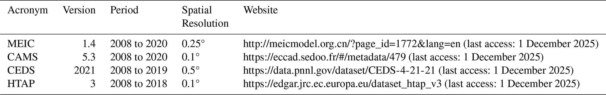
Based on the above considerations, we selected four anthropogenic emission inventories (Table 1) that include one regional (national) and three global emission inventories. These are:

1. The Multi-resolution Emission Inventory for China (MEIC version 1.4). MEIC is a national inventory for mainland China developed by Tsinghua University and updated to the year 2020 (Zheng et al., 2018, 2021a). Due to the 22 emission sectors provided in the newer version 1.4 (released in 2023), we use MEICv1.4 to improve sectoral comparisons in our study. The previous version, MEICv1.3, has been widely used in a number of research studies to date (Liu and Wang, 2020; Wang et al., 2024). We also provide comparisons of emission amounts (NO_x, CO, and NMVOCs) between MEICv1.3 and MEICv1.4 in Fig. S2. MEICv1.4 data used in this study are provided in Zenodo (Zhang, 2025b). Absolute differences of annual averages (MEICv1.3 values minus latest MEICv1.4 values over MEICv1.3 values) were calculated and then expressed as percentages with respect to the annual average emissions in the more recent emission inventory. The differences in total pollutant emissions in China between the two versions were found to be less than 5 %, and differences between other versions of inventories follow the same calculation.

2. The Community Emissions Data System (CEDS, version 2021). This is a global emission inventory for the Coupled Model Intercomparison Project Phase 6 (CMIP6) (Hoesly et al., 2018; Feng et al., 2020; Smith et al., 2022). CEDSv2021 provides detailed descriptions of emission sectors and IPCC sector codes, which facilitates inter-comparison of sectoral emissions (Hoesly et al., 2024). Comparisons between CEDSv2021 and the previous version, CEDSv2019, suggest that there are only slight differences (<3 %) in the emissions of ozone precursors in China (Fig. S4), therefore CEDSv2019 is not included in further analysis.

3. The Copernicus Atmosphere Monitoring Service emissions (CAMS, version 5.3). This dataset is based on the Emission Database for Global Atmospheric Research (EDGAR version 5) until 2018, and projected to 2022 by using the linear slopes of CEDS sectoral emissions from 2015 to 2019 (Granier et al., 2019; Doumbia et al., 2021; Soulie et al., 2024). We also compared pollutant emissions in China in CAMSv5.3 and the latest version of EDGAR, EDGAR v6.1 (Fig. S3). CAMSv5.3 data used in this study are provided in Zenodo (Zhang, 2025b). Results indicate the similarity between the two emission inventories, with differences ranging from 4 % to 7 % for total annual emission for China, from 2008 to 2020. The uncertainties of CAMs extrapolation method will also be discussed in Sect. 3.1. Thus, EDGAR v6.1 was not selected for this study.

4. Hemispheric Transport of Air Pollution (HTAP, version 3). HTAP is a newly published global emissions inventory that incorporates the Regional Emission Inventory of Asia (REAS, version 3.2.1) for pollutant emissions in East, Southeast, and South Asia (including China) (Kurokawa and Ohara, 2020; Crippa et al., 2023). HTAPv3 includes more comprehensive sectoral emissions than REASv3.2.1, including domestic and international aviation and shipping, waste emissions, and agricultural waste burning from EDGAR (Monica, 2023). HTAPv3 reports higher emissions than REASv3.2.1, by 2.5 Tg (8.8 %) for NO_x and by 2.5 Tg (8.7 %) for NMVOC, while the difference in CO emissions between the two inventories is less than 0.5 % (Fig. S5 and Sect. S4). In addition, the newly released HTAPv3.1 inventory (Guizzardi et al., 2025) and MIXv2 inventory (Li et al., 2024) incorporates the MEICv1.4 inventory. Our final dataset–CINEI aims at methodological improvements and provide a more comprehensive coverage of emission sectors than MIXv2 and HTAPv3.1, especially with the inclusion of the agriculture and aviation sectors. In addition, CINEI’s detailed NMVOC speciation that is fully compatible with the MOZART chemistry mechanism enhances its suitability for global atmospheric modeling and its versatility relative to other regional inventories, including MEIC, REAS, and MIXv2. Figure S6, showing a comparison of the interannual variation in NO_x, CO, and NMVOC emissions over China among CINEI, MIXv2, and HTAPv3.1 inventories for the overlapping period (2010–2017), demonstrates only minor discrepancies among the inventories. Annual emissions in HTAPv3.1 are 2.1 % higher than CINEI (ranging from −0.8 % to +5.8 % across different species), while MIXv2 emissions are consistently 3.2 % lower (ranging from −1.6 % to −6.1 %) (see further discussion in Sect. S5).

Table 1 List of emission inventories considered for integrated inventory

2.2 Harmonizing and integrating emission inventories

In order to improve comparability and build on the strengths of national (MEIC) and global emission inventories, our goal was to develop an integrated emissions was to develop an integrated emission inventory for China (CINEI) based on harmonized emission inventories, but with emissions from all activity sectors in China following the IPCC definitions of emission sectors and updated NMVOC speciation with observation-based, localized profiles. To do this, we harmonized the emission inventories by unifying the definition of emission sectors, spatial resolutions, and NMVOC speciation between the MEIC and global emissions. The framework for creating the harmonized CINEI is shown in Fig. 1a, and the Python code for this processing can be accessed on the Zenodo website (https://doi.org/10.5281/zenodo.15000795) and archived by Zhang (2025a). Further details are provided below:

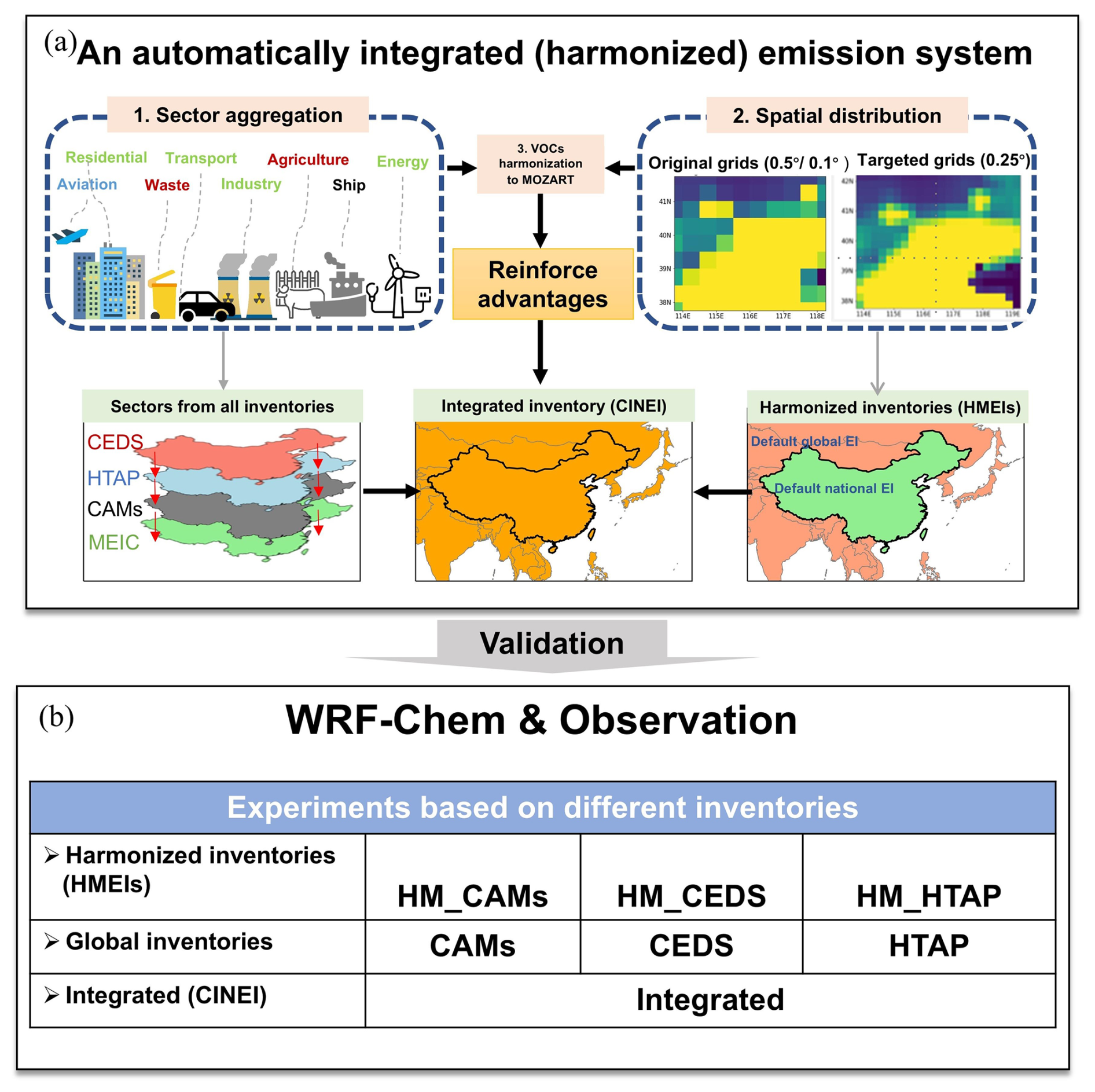
Figure 1 Representation of the framework of an integrated (harmonized) emission inventory system (top two panels) and its evaluation scheme (bottom panel). Figure 1a illustrates the procedure for the construction of the harmonized and integrated (CINEI) emission inventories, which is explained in Sect. 2.2. Figure 1b shows the WRF-Chem experiments performed to validate the emission inventories, with detailed explanations in Sect. 2.3.

2.2.1 Step 1 – Sectoral mapping: Harmonizing emission sectors between the national and global emission inventories.

The classification of emission sectors often differs between different emission inventories. To compare sectoral emissions and harmonize emission sectors, we first need to use emission sector mapping tables to establish the correspondence between the emission sector definitions in the selected emission inventories and the standard sub-sector codes of the IPCC (Intergovernmental Panel on Climate Change; IPCC, 2006), as shown in Fig. S8. The correspondence of emission sectors is based on their definitions for each inventory, which are collected through extensive literature and data documentation on the official website (Granier et al., 2019; Li et al., 2024; Crippa et al., 2023). Eight sectors are defined in the harmonized and integrated emission inventories, including:

1. Transportation. Emissions from both road and non-road transport. Emissions are quantified based on fuel consumption, and vehicles contributing to such emissions include heavy and light trucks, rail vehicles, passenger cars and motorcycles, etc. Emissions from international shipping and aviation are excluded from this emission sector.

2. Residential. Emissions from small-scale residential and commercial activities, including heating, cooling, lighting and cooking, as well as auxiliary engines used in houses, commercial buildings, service institutes, etc.

3. Power. Emissions from electricity generation, commonly driven by large-scale intensive fuel combustion. The incineration of waste in waste-to-energy plants is also included.

4. Industry. Emissions from by-product industrial processes, including emissions from solvent volatilization, cement, iron and steel production, fugitive emissions, refinery emissions and other fuel-related emissions. This sector also covers emissions from volatile chemical products (VCPs) such as petrochemical products, coatings, and printing inks. These sources emit high-reactivity species such as m/p-xylene, propene, and toluene, which are important contributors to ozone formation.

5. Agriculture. Emissions from agricultural soil, manure management, cultivation, and agriculture waste burning. Agriculture waste burning includes straw burning, and excludes savannah burning (Crippa et al., 2023). Besides, transportation emissions due to the usage of agricultural vehicles (such as fishing boats) are also included here.

6. Waste. Emissions related to solid waste disposal and wastewater treatment.

7. Aviation. Emissions from aviation activities, including the take-off, cruising and landing of aircraft.

8. Ships. Emissions from shipping activities on both oceans and inland waterways.

Table 2 lists the data sources for CINEI's sectoral emissions and the missing sectors in existing inventories. By following the IPCC sector definitions, we were able to identify sectors that were omitted from certain emission inventories (see Fig. S8). We selected the emission sectors from different inventories based on three principles, in the following priority order: (1) whether the sectors included complete sources (sub-sector) and species, as indicated by “Completion of sub-sectors and species” in Table 2; (2) whether the sector used high-quality and updated underlying data for calculating emissions, as indicated by “Better underlying data” in Table 2; and (3) whether the emission estimations for the sectors considered the mitigation measures implemented in China (as discussed in Sect. S2), which is indicated by “Incorporation of pollution mitigation measures” in Table 2.

Table 2 Data sources of CINEI sectoral emissions and mapping with global emission inventories

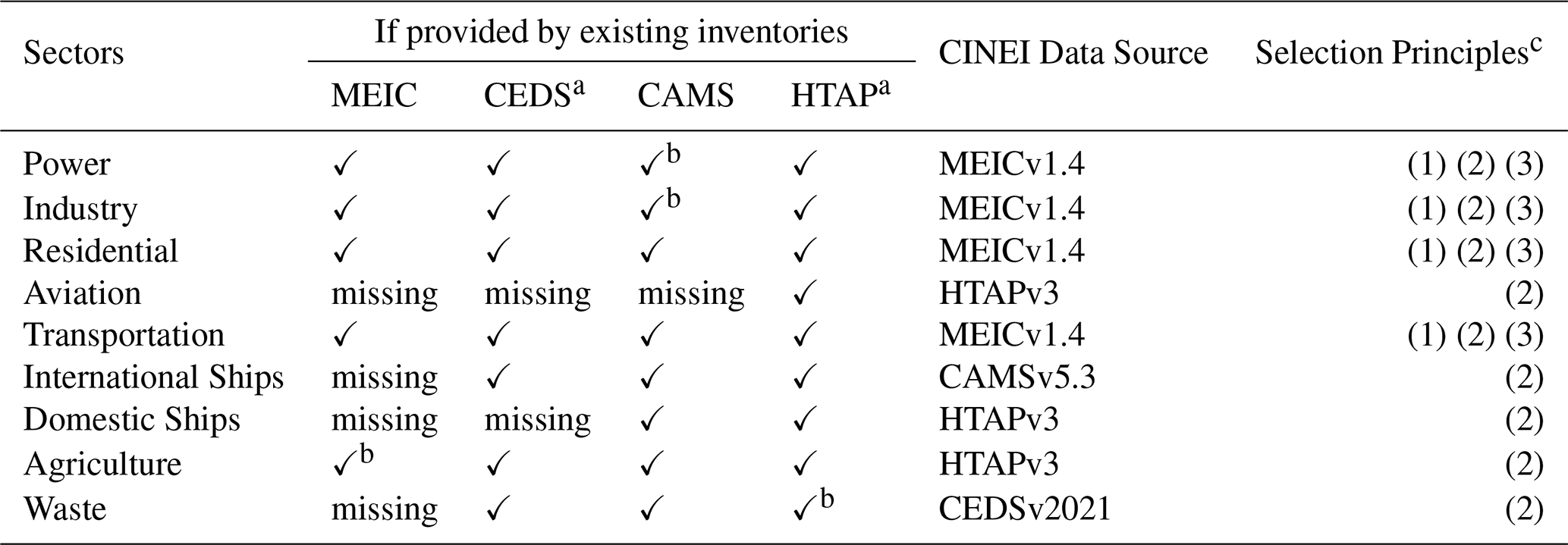
^a As emissions from HTAP and CEDS are not extended to 2020, we use a linear regression of the emissions from 2008 to 2018 (2019) for HTAP (CEDS) and extrapolate to 2020 for CINEI. ^b Indicates that the emissions inventory provides parts of the sectoral emissions but misses some subsectors suggested by the IPCC report. Details on IPCC subsectors and a comparison to each inventory are listed in Fig. S8. ^c The selection principles are prioritized in the following order: (1) Completion of sub-sectors and species, (2) Better underlying data, and (3) Incorporation of pollution mitigation measures.

For CINEI, we retained the emissions from the four existing sectors (transportation, residential, industry, and energy) that were utilized in MEIC, as these sectors adhere to the three principles. As detailed in Sect. S2, MEICv1.4 employed local emission factors and activity data and included a parameter for abatement estimation (Sect. S2 and Table S1). The emission peak year is consistent with the year of mitigation implementation (see Sect. S9).

We integrated emissions from various global inventories for the four missing sectors to ensure comprehensive sectoral coverage and consistency between national and global emission inventories. Specifically, we used emissions from HTAP for aviation and domestic shipping. We opted for HTAP's data for domestic shipping because its inventory provides an independent sub-sector for inland shipping, whereas inland shipping emissions from CAMS are not very complete due to the limited use and coverage of the Automatic Identification System (AIS) on inland waterways. We incorporated ocean shipping emissions from CAMS, which refines data using the Ship Traffic Emission Assessment Model (STEAM3), providing a more detailed representation of shipping routes and emissions (Johansson et al., 2017). For the agriculture and waste sectors, we utilized data from CEDS because its agricultural emissions are more comprehensive than those of MEIC (which only considers NH₃, and its waste emissions are more complete than those from sources from other inventories (Fig. S7).

We also analyzed the changes in ozone precursor emissions in China. The trend in emissions from a sector x is calculated for the studied period of 2008 to 2020 using the Eq. (1).

$$\begin{array}{}\text{(1)}& \begin{array}{rl}{T}_x& ={\displaystyle \frac{E_{x,\mathrm{2008}}}{{\sum }_n^{k=\mathrm{1}}{E}_{k,\mathrm{2008}}}}\times \left|{\displaystyle \frac{E_{x,\mathrm{2020}}-E_{x,\mathrm{2008}}}{E_{x,\mathrm{2008}}}}\right.\\ & \left.-{\displaystyle \frac{{\sum }_n^{k=\mathrm{1}}{E}_{k,\mathrm{2020}}-{\sum }_n^{k=\mathrm{1}}{E}_{k,\mathrm{2008}}}{{\sum }_n^{k=\mathrm{1}}{E}_{k,\mathrm{2008}}}}\right|,\end{array}\end{array}$$

where:

• T_x is the relative changes of emissions from the emission sector x in the end years for global inventories that stops at 2018 for HTAP and 2019 for CEDS, we extrapolate the data to year of 2020 through linear regression,

• $\frac{E_{x,\mathrm{2008}}}{{\sum }_{k=\mathrm{1}}^n{E}_{k,\mathrm{2008}}}$ is the relative changes of emissions from the emission sector x in the end years for global inventories that stops at 2018 for HTAP and 2019 for CEDS, we extrapolate the data to year of 2020 through linear regression,

• $\frac{E_{x,\mathrm{2020}}-E_{x,\mathrm{2008}}}{E_{x,\mathrm{2008}}}$ gives the relative change in emission from sector x from 2008 to 2020,

• $\frac{{\sum }_{k=\mathrm{1}}^n{E}_{k,\mathrm{2020}}-{\sum }_{k=\mathrm{1}}^n{E}_{k,\mathrm{2008}}}{{\sum }_{k=\mathrm{1}}^n{E}_{k,\mathrm{2008}}}$ gives the relative change in total emissions from 2008 to 2020.

We defined key sectors as those with an obvious influence on changes in total national emissions of a pollutant. We identified key sectors based on the following two criteria: (1) they show a clear increasing or decreasing trend in line with total emissions; (2) the total contributions of the key sectors can explain more than 95 % of the total emissions changes. We have adopted this calculation from Intergovernmental Panel on Climate Change (IPCC) (2006).

2.2.2 Step 2 – Uniform spatial resolution: Re-gridding emission data to the same spatial resolution.

The global inventories under consideration have different horizontal resolutions, ranging from 0.1 to 0.5° in both longitude and latitude. To ensure a consistent integration, we need to align their resolutions. Therefore, to match the resolution of the MEIC, we spatially interpolated all global inventory data to the grid coordinate with a resolution of 0.25° × 0.25° (latitude × longitude). We used ‘Conservative’ algorithms for the adjustment, which ensures that the quantity of emissions in the new grids does not change compared to that in the old grids. The emissions in 180 mass in the new grid cell k (denoted as E_k) are quantified by Eq. (2),

$$\begin{array}{}\text{(2)}& E_k=\int \underset{A_k}{\int }e\left(r\right)\mathrm{d}A,\end{array}$$

where e(r) is the emission density in the old grid cell that intersects with this new grid, and A_k indicates the areas of intersections between two grids (Dukowicz, 1984). These integrals must be calculated for all cells of the new mesh.

2.2.3 Step 3 – NMVOC speciation mapping: Aligning NMVOC emissions in all emission inventories to the same speciation

NMVOC emissions are assigned different speciations in different inventories. NMVOC speciation in regional and national inventories (e.g., MEIC and REAS) often follows chemical mechanisms widely used in models, such as the Carbon Bond Mechanism (CBM) (Gery et al., 1989), the Regional Acid Deposition Model gas-phase chemical mechanism (RADM) (Iacono et al., 2008), and the State Air Pollution Research Center (SAPRC) (Carter, 2015). However, global inventories often speciate NMVOC species according to the Model for Ozone and Related chemical Tracers mechanism (MOZART) (Li et al., 2014; Huang et al., 2017). We also assumed MOZART speciation for the integrated inventory (Table S4). This facilitates comparison of speciated NMVOC emissions with global inventories and application in global models, because the MOZART speciation is also used in global inventories and global CTMs (Lamarque et al., 2010; Huang et al., 2017; Emmons et al., 2020). To perform the integration of emissions of specific NMVOC species and to meet the requirements of simulations by CTMs, it is essential to make the NMVOC speciation in different emission inventories consistent. For harmonized inventories, we applied a mapping table (Table S4) to align the MEIC NMVOC lumped species categories with those in the global inventories, and the MOZART speciation is applied to NMVOC emissions in all inventories after mapping. For the CINEI, we updated the NMVOC speciation by applying recently reported localized source profiles and lumped NMVOC emissions following the NMVOC categories in the MOZART mechanism (Emmons et al., 2020). CINEI inventory with MOZART NMVOC speciation can be used in a wide range of air quality studies, as well as in regional and global CTMs. Examples include the Weather Research and Forecasting (WRF) model coupled with Chemistry (WRF-Chem), the Community Earth System Model (CESM) and the Multiscale Infrastructure for Chemistry and Aerosols (MUSICA) (Dai et al., 2023; Mariscal et al., 2025; Danabasoglu et al., 2020; Dai et al., 2024). Such compatibility enhances the versatility of CINEI relative to other regional inventories, including MEIC, REAS, and MIXv2. Total NMVOC emissions from different sectors were assigned to more than 80 specific VOC species based on NMVOC speciation profiles reported by Mo et al. (2016) and Sha et al. (2021) (details in Tables S5 and S6). These profiles describe well the recent speciation of NMVOC emissions in China based on representative measurements (Li et al., 2014). In order to evaluate and compare the impact of different NMVOC species on ozone formation, ozone formation potentials (OFPs) are calculated in this study. For the NMVOC species j, its OFP value is calculated by Equation (3):

$$\begin{array}{}\text{(3)}& \text{OFP}\left(j\right)=\text{EVOC}\left(j\right)\times \mathrm{MIR}\left(j\right),\end{array}$$

where EVOC(j) is the emissions of j, and MIR(j) is the maximum incremental reactivity of j, defined as the potential maximum ozone production per consumption of j under high-NO_x conditions (Carter, 1994). The MIR values used in this study were derived from Carter (2015) and are listed in Table S6. The MIR indicates the amount of ozone growth as the incremental emission of NMVOC species increases, and is unitless. Therefore, the unit of OFPs should be mass based and here we use Tg-O₃.

2.2.4 Step 4 – Emissions’ harmonization and integration: Spatial harmonization and integration of emissions by species and sector

In the previous three steps, the selected inventories (MEIC, CEDS, CAMS, HTAP) are transformed into new ones with consistent sector types, spatial resolutions, and NMVOC speciation (MOZART). This step harmonizes and integrates the national and global inventories and improves the compatibility of the integrated inventory with the chemical mechanism of the CTM. We focus on anthropogenic pollutant emissions in East Asia (70.125 to 149.875° E and 10.125 to 59.875° N), which is gridded in 320×200 grids. National and global inventories in this area are combined to produce Harmonized Emission Inventories (HMEI) and CINEI, the details of which are presented below:

• Harmonized emission inventories (HMEI). In these inventories, anthropogenic emissions within Mainland China are derived from the standard Chinese national inventories, MEIC and those outside of China are from the global emission inventories. Based on the type of global inventory used in the processing, three harmonized global emission inventories were created: HM_CAMS (harmonized MEIC with the CAMS global inventory), HM_CEDS (CEDS), and HM_HTAP (HTAP) when using MEIC.

• Integrated emission inventory (CINEI). Based on the harmonized emission inventories, CINEI also includes all emission sectors and updated NMVOC emissions speciated according to the MOZART chemical scheme (Zhang et al., 2025). As mentioned above, emissions from four sectors, including ships, waste, aviation and agriculture, are missing in the MEIC. In the CINEI, emissions from these missing sectors in China are derived from the global emission inventories as explained in Step 1 and shown in Table 2. The difference between CIENI and HMEI lies in the new sectors added to CIENI, which increase total emissions. Furthermore, the additional emission sectors affect the composition of specific local emissions, which will be discussed in later sections.

To consolidate the data fusion from national to global emission inventories at spatial scales, we calculated the Monte Carlo uncertainty for sectoral emissions for the global inventory (CEDS) and the regional CINEI (Lee et al., 2024). We randomly select 10 000 samples from 64 000 values (200 × 320), calculate the standard deviation of the samples, and repeat this step 1000 times until the standard deviation does not change. We use the standard deviation to represent Monte Carlo uncertainties, and if the standard deviations of the global and CINEI inventories are of the same magnitude, we assume that the data fusion is reliable (Heuvelink and Brus, 2009).

2.3 Evaluating emission inventories Using WRF-Chem Model

To evaluate the performance of the harmonized and CINEI inventories, we used the Weather Research and Forecasting model with Chemistry (WRF-Chem, version 4.3.2; Skamarock et al., 2019; WRF Model Development Team, 2025) to run simulations for our region of interest with different inputs of anthropogenic emissions and compared the model results with measurements of ozone (O₃), carbon monoxide (CO), and nitrogen dioxide (NO₂). We performed simulations using each of the three global emission inventories (CAMS, CEDS, HTAP), three harmonized inventories (HM_CAMS, HM_CEDS, HM_HTAP), and CINEI (Fig. 1b), and for two different simulation periods, January (representing winter) and July (representing summer) 2017. In addition, the MIXv2 inventory incorporates the MEICv1.4 inventory for Asia, which has high lumped speciation and missing aviation emissions. Its modeling performance with the same setup for July 2017 is discussed in the Supplement (Fig. S29 and Table S22).

We used the same model setups for all experiments (Table S7). Specifically, we set up two-way nested simulation domains with spatial resolutions of 36 km×36 km and 12 km×12 km (Fig. 2). Specifically, the inner domain includes the major populated areas of eastern China. The domain has a dense network of air quality monitoring sites (Fig. 2) and meteorological monitoring sites (Fig. S9). The chemical initial and boundary conditions for the outer domain were derived from the 6-hourly output of the CAM-chem model (Lamarque et al., 2010), while for the inner domain they were extracted from the results of the simulation in the outer domain. MOZART (Emmons et al., 2020) was used to simulate gas-phase chemistry and reactions, and MOSAIC (MOdel for Simulating Aerosol Interactions and Chemistry; Hodzic and Knote, 2014) was set as the aerosol scheme. Biomass combustion emissions were taken from the FINN (Fire INventory from NCAR, version 1.5) inventory (Wiedinmyer et al., 2011), and biogenic emissions are estimated using the Model of Emissions of Gases and Aerosols from Nature (MEGAN, version 2.1) (Guenther et al., 2012). We set the spin-up time to 6 d before the study periods to avoid the influence of imbalanced chemical initial conditions on the simulation results.

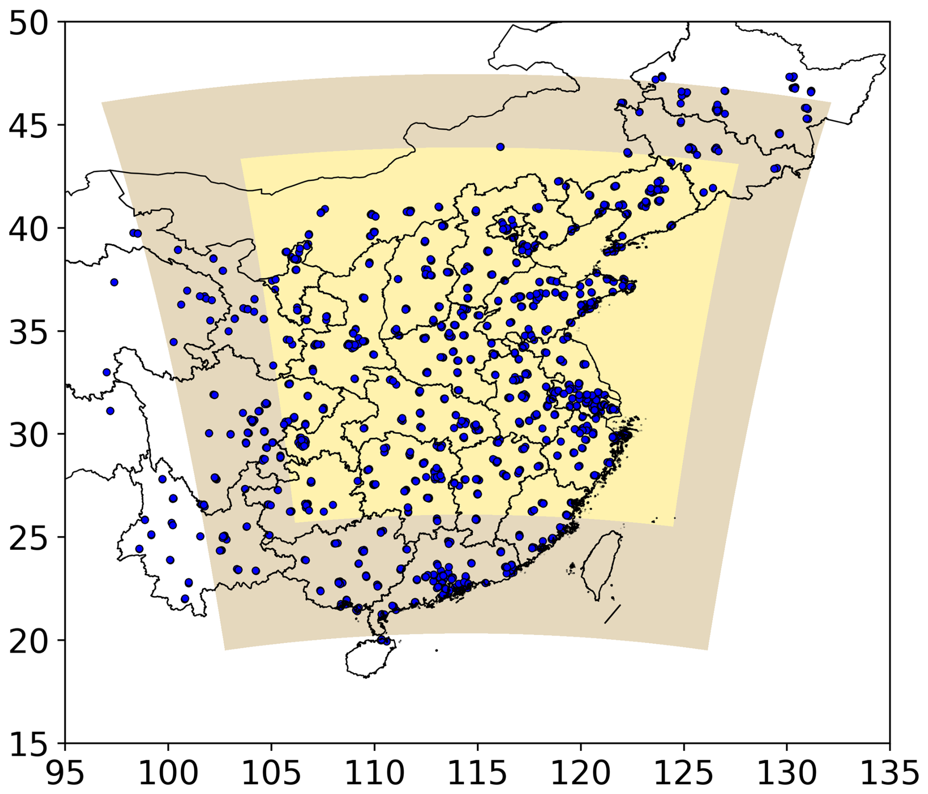
Figure 2 Model domains employed for WRF-Chem simulations in eastern China. The horizontal resolution of the outer Domain 01 (depicted in gray) is 36 km, featuring 75×86 grids, including a total of observed 1372 sites (in dark blue). The inner Domain 02 (illustrated in yellow) has a higher horizontal resolution of 12 km, with 160×166 grids, covering observed 969 sites (in dark blue).

To evaluate the model performance across all experiments, we compared the modeled hourly averaged mixing ratios of O₃, CO, and NO₂ at the finer scale with corresponding observations at 969 national air quality monitoring sites. The modeled meteorological variables, including temperatures at 2 m, wind speeds and directions at 10 m, were also validated with the 3 h observational data set at 136 sites obtained from the National Centers for Environmental Information (https://www.ncei.noaa.gov/, last access: 1 December 2025). Seven statistical metrics were used to determine the performance of the model. The metrics include normalized mean bias (NMB), mean normalized bias (MNB), mean fractional bias (MFB), mean normalized absolute error (MNAE), mean absolute error (MAE), root mean square error (RMSE), and Pearson correlation coefficient (R) (Brasseur and Jacob, 2017). Table S8 provides information on their functions.

3 Results and discussion

3.1 Sectoral emissions and comparison

CINEI shows the comprehensive sectoral anthropogenic emissions and reveals significant changes in ozone precursor emissions (NO_x, CO and NMVOCs) in China (Fig. 3a–c). These include the decrease in NO_x emissions (−0.9 ± 2.9 Tg yr⁻¹) since 2012 and CO emissions (−7.0 ± 23.4 Tg yr⁻¹) since 2008 and the increase of NMVOC emissions (0.4 ± 1.0 Tg yr⁻¹) from 2008 to 2019. CINEI also showed a slight decrease in 2020 due to the COVID-19 shutdown (Zheng et al., 2021a). In general, the major sectors in the global inventories show a greater divergence from the national inventories. There is a of approximately 5 % for NO_x of power generation with respect to the total emissions of CINEI, and a deviation of more than 10 % for HTAP and CAMS CO from residential activities. The deviations in the totals are minimal and the sectors are more comprehensive by including the main sectors from the national inventory and key sectors (ships, waste, etc., as discussed in Sect. S8 and Tables S12–S14). Global inventories (HTAP and CEDS) agree well with the national (MEIC) in terms of total emission levels and multi-year changes in China (Fig. 3g–i). However, emissions in CAMS show notable differences from those in other inventories: CAMS estimates lower NO_x and CO emissions in China before 2014; CAMS displays the variation without rapid reduction during the study period (Fig. 3d–f).

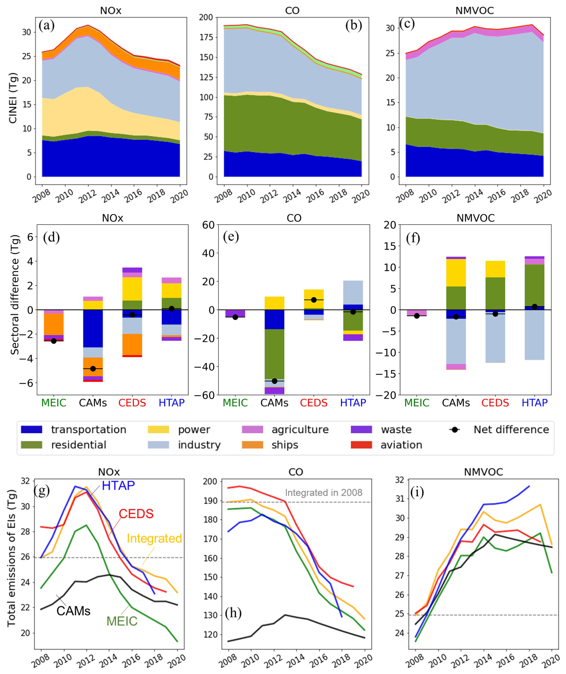
Figure 3 The top panels (a–c) show the interannual variability of NO_x (NO₂), CO, and NMVOC emissions across eight aggregated sectors in the CINEI, and all data are listed in Tables S9–S11. The middle panels (d–f) depict the averaged annual differences from 2008 to 2018 in sectoral emissions between each of the four inventories and CINEI (existing inventories minus CINEI). Sectoral emissions are indicated by bars and total emissions by dots. The findings are based on the mean differences from 2008 to 2018, and the results for each year are shown in Fig. S13. The bottom panels (d–f) present the interannual variability of total NO_x (NO₂), CO and NMVOC emissions in China from the CINEI (in orange) and four selected emission inventories (MEIC in green, CAMS in black, CEDS in red, and HTAP in blue). Total emissions from 8 sectors used from multiple inventories are provided in Tables S9–S11.

CINEI also provides the amount of emissions from eight anthropogenic sectors (Fig. 3a–c). The main sectors of the CINEI in China include industry (NO_x, CO, NMVOCs), transportation (NO_x, CO, NMVOCs), and transport (NO_x, CO, NMVOCs), power (NO_x) and residential (CO, NMVOCs). Compared to MEIC (harmonized inventories) for China, CINEI total emission on annual average includes the contributions of the ships sector to NO_x emissions (2.7 Tg), the waste sector to CO emissions (5.2 Tg), and the agricultural sector to NMVOC emissions (1.4 Tg) (Fig. 3d–f). Ignoring these emissions can lead to bias in the estimation of anthropogenic emissions and in the simulation of ozone (von Schneidemesser et al., 2023). Differences in sectoral emissions (CINEI minus other inventories) are evident in major and omitted sectors (Fig. 3d–f). In general, emissions from the power sector are often higher in the three global inventories, while those from the transport sector are mostly lower. The apparently lower NO_x from transport and CO from residential emissions in CAMS (and EDGAR) are mainly due to underestimated contributions. Although CEDS provides total emission estimates closer to those of CINEI for China, there are still notable differences in the contributions of certain sectors. The uncertainties of the CAMs extrapolation method for the main sectors are between 30 % and 60 % (see Sect. S6 and Table S3). One exception of power uncertainty is over 100 %, likely due to the systematic uncertainty in the sector definitions and mapping. In particular, the energy and residential sectors contribute more to NO_x emissions, but lower emissions from shipping and industry offset these increases. Higher NMVOC emissions from the power sector are offset by those from the industry sector. This is similar to the comparison of sectoral emissions in HTAP and CINEI.

We also analyzed the contributions of sectoral emissions to changes in total emissions and identified the key sectors for emission changes of each pollutant. Table S15 summarizes the linear trends (slopes) of 8 sectoral emissions for NO_x, CO, and NMVOCs from 2008 to 2020, and the piece-wise slopes for sectoral emissions that show changes with increases followed by decreases (Table S16). The power sector is the main driver of the decrease in NO_x emissions for China, contributing 49 % to the downward trend with a linear reduction of −0.33 yr⁻¹. In the CINEI, emissions from the power and industrial sectors (for NO_x) and the residential sector (for CO) started to decline after peaking in 2013 (see Table S15). This timing aligns with the emission reduction measures implemented, starting with the 12th Five-Year Plan in 2011 (12th Five-Year Plan, 2011, see Sect. S2). The improved reflection of mitigation actions in the MEIC inventory comes from accounting for factors such as technology adoption and abatement efficiency (see Sect. S2 and Table S1), such as energy transition to cleaner resources (Yan et al., 2023). Over the study period, the sectors responsible for the largest reductions in CO emissions were industry (60 % of the reduction), residential (29 %), and transportation (16 %). The main contributors to the observed linear declines in CO were industry (39 % contribution, −3.6 Tg yr⁻¹), residential (22 %, −1.8 Tg yr⁻¹), and power (13 %, 0.14 Tg yr⁻¹). CO emissions from more specific sources, including the petrochemical industry, cooking, and gasoline-powered vehicles, also show significant reductions in MEIC v1.4 (Fig. S11). In addition, industry is driving the increase in NMVOC emissions, despite the decrease in NMVOC emissions from the residential and transportation sectors. These NMVOC emissions are associated with industrial painting, iron and steel industry, and architectural coatings in MEIC v1.4 (Fig. S12). Thus, more efforts are warranted in the future to control NMVOC emissions from industrial processes in China.

Ozone precursor emissions from four key sectors not included in the MEIC inventory (shipping, waste, agriculture, and aviation) are included in the CINEI inventory and are identified as key contributors (see Table S15 and Sect. S8). The shipping sector is a major contributor to NO_x emissions in China, with a linear emission increase of +0.07 Tg yr⁻¹, making it the third-largest driver of the total NO_x trend at 21 %. Aviation follows as the fourth-largest contributor to NOx with 3 % (+0.01 Tg yr⁻¹), while waste accounts for the fourth-largest share of the CO trend at 13 % and also shows a rising trajectory (+0.15 Tg yr⁻¹). For comparison, NOx emissions from shipping in the HTAP inventory also display an upward trend of +0.1 Tg yr⁻¹(Tables S12–S14), which appears to counteract reductions from the energy sector. In summary, our findings indicate that shipping, waste, aviation, and agriculture are key sectors that influence overall trends, often showing increases where other major sectors have declined.

3.2 Speciation of NMVOCs emission

The increase in NMVOC emissions is a potential contributor to severe ozone pollution in China (Li et al., 2019; Zhang et al., 2021). Individual NMVOC species often differ in the amounts emitted and in their ozone formation potential, and thus contribute differently to ozone formation. We ranked the top 20 NMVOC species in China according to their mean annual emissions in CINEI and quantified their OFPs values (Fig. 4a). These NMVOCs species cumulatively contribute to more than 85 % of the total OFPs by NMVOCs emissions, indicating their notable influence on ozone pollution. In general, NMVOCs species with more abundant emissions tend to contribute more to OFPs, such as m/p-xylene and toluene, which together have an OFP value of 23.1 Tg-O₃ on an annual average from 2008 to 2020 (23.4 % of the total OFPs). Propene, o-xylene and ethene, with higher OH reactivity (characterized by their MIR values), also have significant contributions to total OFPs (propene 13.9 Tg-O₃ and 14.1 % in percentage contribution to total OFP, o-xylene 7.1 Tg-O₃ and 7.2 %, and ethene 6.9 Tg-O₃ and 6.1 %). However, high emissions of ethylbenzene and styrene (10 % of total NMVOC emissions) contribute only 7.2 Tg-O₃ (6 %) to the total OFPs due to their low reactivity. Regarding the OFPs of different NMVOC groups, aromatics and alkenes contribute to 75 % of the total OFPs as shown in Fig. S14. This result is in good agreement with previously reported results (Li et al., 2019; Wu et al., 2022). The OFPs values in VOCs categories are also compared with the result of previous studies (Table S17). The emission and OFPs of all NMVOCs species on annual averages also for mainland China are shown in Tables S20 and S21.

Figure 4 (a) Mean annual emissions (blue bars in Tg yr⁻¹) and OFPs (yellow line in Tg-O3 yr⁻¹) of the top 20 NMVOCs species in CINEI (ranked by emission amount). Error bars at the top of the columns represent the standard deviations of the emissions from 2008 to 2020. (b) Sectoral contributions to the emissions of the top 20 NMVOC species. Emissions and OFPs of all NMVOC species in 8 sectors are provided in Tables S20 and S21 respectively.

Targeting the emission sectors most related to NMVOC species with high OFP values may be efficient for ozone mitigation. The sectoral contributions to the top 20 NMVOC species are shown in Fig. 4b. M/p-xylene, toluene, propene and o-xylene emissions are mainly derived from the industrial sources (∼ 70 %). This involves their usage as solvents in industrial processes (e.g., industrial painting and architectural coatings). The residential sector also has an important contribution to these NMVOC species, accounting for 20 %–30 %. Ethene emissions show different characteristics: besides the considerable contributions of the industrial and residential sectors, agriculture also accounts for a large proportion (32 %) as does transportation (25 %), indicating the contributions of fishing and harvesting and diesel vehichles. For the other NMVOC species among the top 20, industry and transportation are mostly the major sources, and therefore NMVOC emission control should focus on the contributions of these two sectors. The agricultural sector is the main source for formaldehyde (52 %) and acetaldehyde emissions (60 %), related to the emissions along with crop burning (including the burning of rice and wheat straw, maize, etc.). Ignoring agricultural NMVOC emissions in anthropogenic emission inventories can lead to underestimated contributions of these species to ozone pollution. Ozone pollution may occur in areas with intensive local agricultural activity.

Total NMVOC emissions and OFPs in China, showed an overall increasing trend from 2008 to 2020, with linear slopes of 0.2 Tg yr⁻¹ (emission) and 1.1 Tg-O₃ yr⁻¹ (OFPs), as shown in Fig. S14. Fourteen of the top 20 species exhibited increasing trends and contributed significantly to OFPs, including m/p-xylene (18 % OFP contribution and 0.04 Tg-O₃ yr⁻¹), propene (18 % and 0.2 Tg-O₃ yr⁻¹), and toluene (10 % and 0.03 Tg-O₃ yr⁻¹) (Figs. S15 and S16). The primary driver for this increase was the industrial sector, particularly processes like industrial painting, iron and steel production, and architectural coating (Fig. S15). To mitigate ozone formation, targeted strategies should focus on industrial emission controls for high-OFP species, particularly aromatics like xylenes and toluene, while continuing to strengthen transportation and residential emission reductions. Furthermore, since formaldehyde and several alkenes showed decreasing trends, policies should maintain these reductions while preventing industrial sector growth from overwhelming overall mitigation efforts through stricter industrial VOC controls and cleaner production technologies. All of the major NMVOC species identified by CINEI show increasing trends within the sectors added from global inventories, namely agriculture, shipping, aviation, and waste. For example, total NMVOC emissions from the agriculture sector are slightly rising by +0.003 Tg yr⁻¹. Key speciated NMVOC emissions from these four sectors, such as ethene (which contributes 8 % to total OFP) and formaldehyde (5 %), also show notable increases. To effectively reduce ozone levels, mitigation strategies should target not only highly reactive species like m/p-xylene, toluene, and propene from industrial sources, but also address emissions from sectors like agriculture and aviation that are often overlooked in national inventories.

To evaluate the NMVOC speciation used in CINEI, we selected 9 hydrocarbon species and used their emission ratios to acetylene (C₂H₂, unit: mol mol⁻¹) for comparison with those in global and national inventories, as well as with observations over China (Fig. S17). We used C₂H₂ instead of CO because C₂H₂ and hydrocarbons are monitored with the same measurement system (GC MS/FID). The in situ measurements of VOC species (in ppbv) were obtained from the literature (Lv et al., 2021; Huang et al., 2022; Li et al., 2022; Song et al., 2021). These data, obtained from megacities (Beijing, Shanghai, etc.) and provincial capitals, are listed in Tables S18 and S19. We extracted emissions at the same locations and dates and calculated the ratios of hydrocarbons to C₂H₂. The selected VOCs have similar atmospheric lifetimes and sources in urban areas, primarily from transportation and industrial emissions. Species treated as a single entity in emission inventories (e.g., ketones) and those not comparable to observations (e.g., oxygenated VOCs) were excluded from the analysis. Our comparison showed that NMVOC speciation from emission inventories is quite uncertain due to the applied source profiles, different sectoral distributions and emission masses. The ratios in the CINEI are closer to the observations, except for ethene and xylene. In contrast, the global and MEIC inventories have lower ratios for alkanes compared to observations, possibly due to misrepresentation of the dominant sectoral emission (solvent or industry) for these species.

When compared to the national inventory (MEIC, with the same ratio as the harmonized inventories), the ethane-to-acetylene and propene-to-acetylene ratios in CINEI are closer to the observed ratios (Fig. S17). These findings may be linked to two factors. First, the ethane-to-acetylene ratio in CINEI is higher than the MEIC ratio resulting from the incorporation of missing sectors (agriculture, aviation, ships, and waste), which contribute 13 % to the total annual average emission and are richer in ethane. Second, the propene-to-acetylene ratio in CINEI is lower than the MEIC ratio despite a 3 % additional contribution from these missing sectors. This may be due to the speciated profile used in CINEI (Mo et al., 2018), which attributes a smaller share of emissions to diesel vehicles (mainly emitting alkenes) and a larger share to gasoline vehicles (mainly emitting alkanes) (Table S20). These findings suggest that using local NMVOC speciated profiles can better capture changes caused by current energy transitions and evolving consumption patterns (Yan et al., 2021). However, the ratios of primary alkenes (ethene) and toluene emission in the MEIC and CINEI exceed the observed values. Alkenes have faster loss rates via OH, which may lead to alkenes from primary source are degraded immediately. Therefore, the observed ratios of alkenes to C₂H₂ may be lower than its emission ratios (MIR >9). Therefore, the speciation of NMVOC emissions. Improving this description would also influence the homogenization of the national inventory with global ones and the application of CTM simulations.

3.3 Harmonizing emissions on spatial scales

Figure 5 shows the spatial distribution of NO_x emissions from the CINEI dataset across eight sectors in East Asia in 2017. For emissions outside of China, we use CEDS emissions for the major sectors because CEDS incorporates national emissions from surrounding countries and is widely used in global CTM models (Hoesly et al., 2018). We chose NO_x as a representative species to analyze the spatial distribution of pollutant emissions in CINEI. Emission maps for other species (SO₂, NH₃, CO, C₂H₆, toluene, and C₂H₄) from CINEI are shown in Fig. S19.

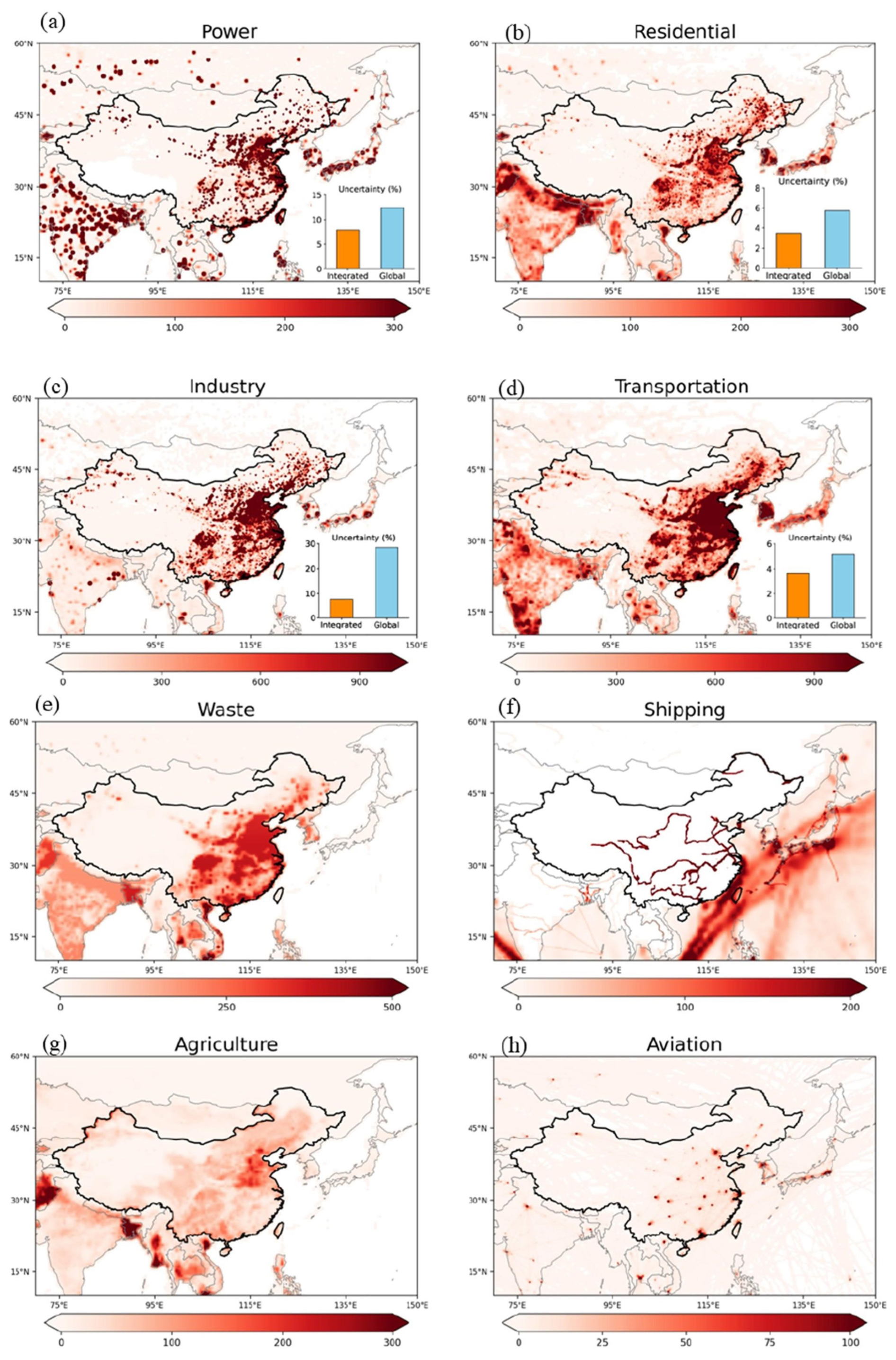
Figure 5 Spatial distribution of NO_x (NO₂) emissions (unit: t grid⁻¹ yr⁻¹) from eight sectors in East Asia in 2017, and for power, residential, industry, transport sectors, we add comparisons of Monte Carlo uncertainties between integrated (CINEI in orange) and global inventory (CEDS, in blue).

Anthropogenic emissions, such as those from the residential, transportation, and waste sectors, tend to be high in densely populated areas of northern and eastern China, Japan, Korea, and India, indicating their close association with human activities (see Fig. S18 for population distribution). NO_x emissions from the energy and industry sectors, which are considered point sources, are characterized by hotspots at sites for electricity generation, solvent volatilization, and cement, iron, and steel production. The convergence of these sectoral data from the national emission inventory and CEDS for surrounding countries in CINEI is tested by Monte Carlo simulations with comparisons to CEDS data. The Monte Carlo uncertainties of the two datasets are of the same order of magnitude, indicating that the possibility density of the CINEI is normal on the spatial distribution and not separated into two datasets.

The distribution of shipping reveals shipping routes in the ocean and inland rivers. Aviation emissions distribution is related to airline connections between different airports, with high values likely occurring near major airports in China. The emissions of other pollutants suggest similar characteristics of spatial distributions (Fig. S19). In addition, harmonized emission inventories used the default emissions for total emission amount from the national inventory, but emissions outside China were taken from the three global inventories. To illustrate the difference in emissions in mainland China and the similarity in emissions outside of China between national and global inventories, the distributions of the paired comparisons (HM_CEDS vs. CEDS, HM_CAMS vs. CAMS, HM_HTAP vs. HTAP) are also shown in Figs. S20–S23.

3.4 Comparisons of simulation results based on multiple anthropogenic emission inventories

To identify the most harmonized inventories suitable for regional simulations over China, the performance of WRF-Chem modeling results based on the national inventory (MEIC) merged into three global inventories (HM_CEDS, HM_CAMS, and HM_HTAP) has been were evaluated. The three harmonized inventories show minimal variation in the averages over the entire domain where the grid contains observed sites (Sect. S12). The normalized mean biases (NMBs) among the three modeling results are 10 % and 40 % for ozone in summer and winter, respectively, −0.5 % in summer and 40 % in winter for NO₂ and −50 % for CO for both seasons (Fig. S24 and Sect. S12). However, HM_CEDS shows better agreement with observations from coastal cities, which have a deeper response to the transport of emissions to mainland China. In contrast, HM_CAMS and HM_HTAP have significant biases. Accordingly, HM_CEDS was selected to represent all harmonized inventories for subsequent modeling comparisons, hereafter abbreviated as HMEI.

Further, we investigate the comparison of experiments' performance between MEIC-based HMEI and global inventories. Modeling ozone mixing ratio using HMEI in January 2017 achieve the smallest normalized mean bias (NMB = −26 %), compared with HTAP (−52 %), CEDS (−33 %), and CAMS (−40 %) (Fig. 7). In July 2017, models using HMEI produced NO₂ and CO bias values (NMB = 0.5 % for NO₂, −34 % for CO) that are closer to zero than results from global inventories (Fig. 6). Comprehensive analysis using several statistical metrics (NMB, MNB, MNAE, MAE, MFE) consistently demonstrates that HMEI delivers superior overall performance compared to individual global emission inventories (Fig. S27–S28). These comparisons of evaluation metrics suggest that CINEI is based on emissions from the main sectors in the MEIC inventory.

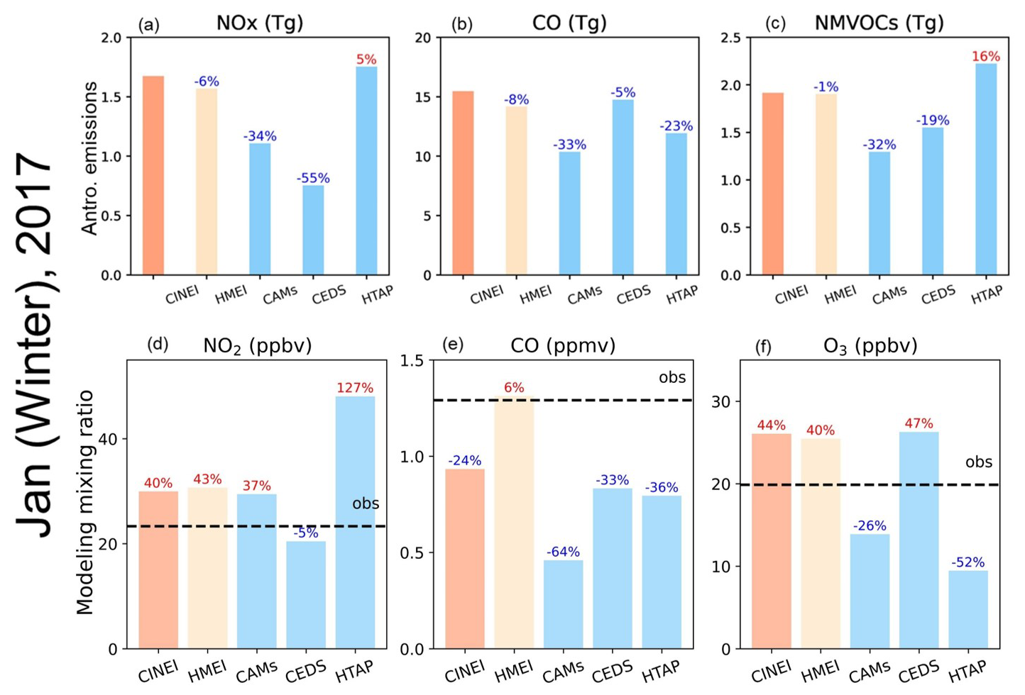
Figure 6 The top panels (a–c) present total anthropogenic emission differences of ozone precursors (NO_x, CO, and NMVOC) for July 2017 between the CINEI, HMEI, CAMS, CEDS, and HTAP inventories using the CINEI integrated emission inventory as a reference. Bottom panels (d–f) show WRF-Chem simulated mixing ratios of O₃, NO₂, and CO for the same month and within the modeling domain (latitudes from 25.5 to 43.6°; longitudes from 103.5 to 127.6°) using the different emission inventories. Individual columns show simulated mean mixing ratios in the model domain for each emission inventory used. The dashed blue lines show average observed mixing ratios calculated using the stations within the specified domain. The numbers on the columns are the normalized mean bias (NMB) against observations for each modeling experiment, and the calculation is expressed in the first line of Table S8. The numbers in red (blue) colors indicate overestimation (underestimation).

Figure 7 Same content with Fig. 6, but in January 2017.

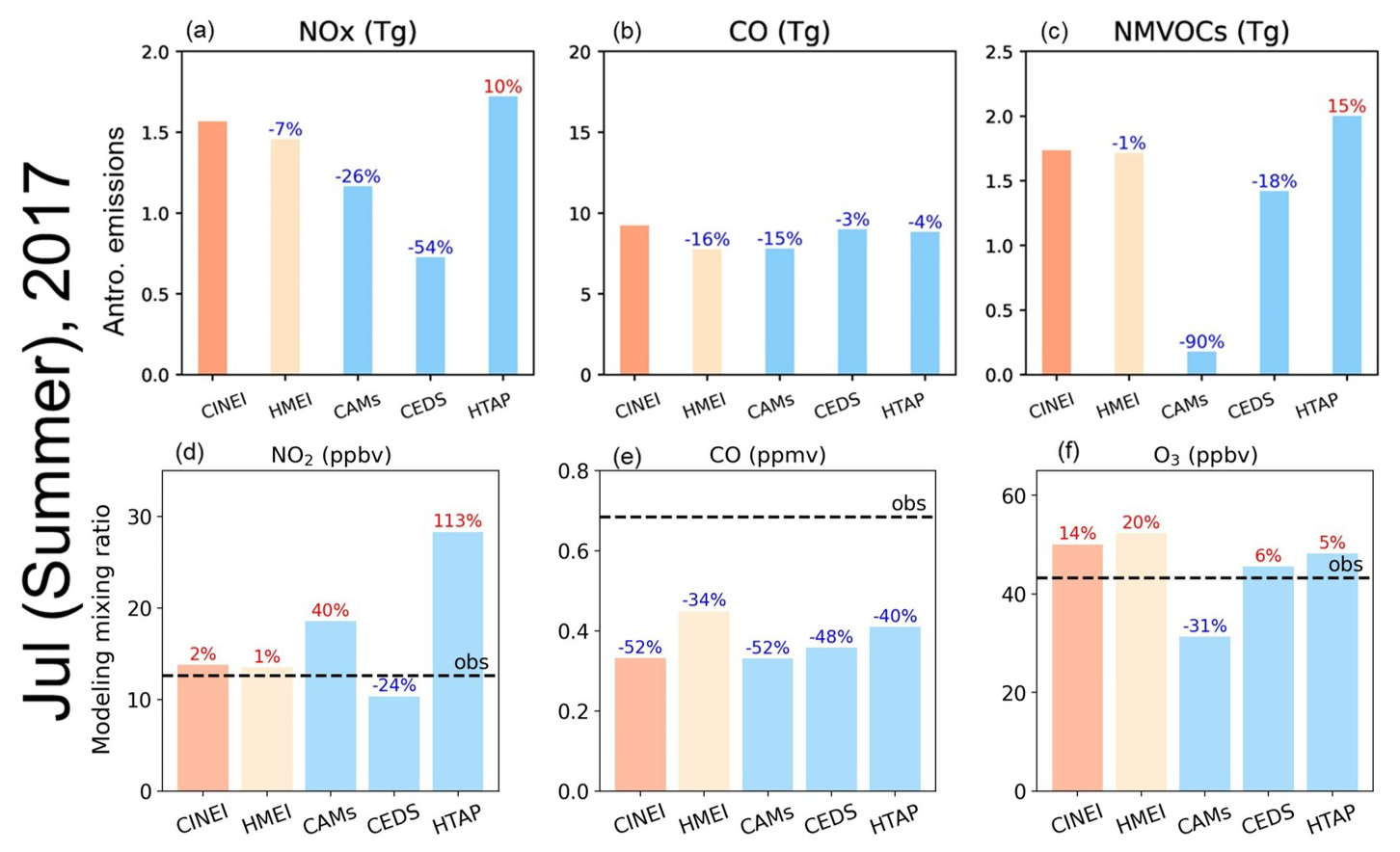
To further evaluate the performance of CINEI, HMEI and global inventories (CAMS, CEDS, HTAP), anthropogenic emissions (NO_x, CO and NMVOCs) are shown in the upper panels of Figs. 6 and 7, and modeling results (O₃, NO₂ and CO mixing ratios) are compared with observations in the lower panels of Figs. 6 and 7. In both months the O₃ mixing ratios are overestimated by CINEI (12 % in summer and 42 % in winter) and HMEI (20 % and 40 % NMB). The NO₂ mixing ratios of CINEI are closer to the observations by about 5 % in summer and 40 % in winter. The differences between the two emission inventories can be attributed to the inclusion of shipping, waste, and aviation emissions, as well as updated NMVOC speciation in the CINEI dataset. Accounting for these sectors results in a modest increase in total emissions (less than 10 %) in CINEI. This change leads to improved model performance, as shown by a reduction in the normalized mean bias (NMB) for O₃ in summer (from 21 % with HMEI to 12 % with CINEI) and for NO₂ in winter (from 24 % with HMEI to 22 % with CINEI). Additional statistical analysis shows that CINEI has superior performance compared to HMEI and global inventories (Sect. S13 and Fig. S27–S28). The MFB for CINEI is ±0.3 in both seasons and the MNAE is less than 0.5, within the ranges suggested in the literature (Zhai et al., 2024). However, the CO mixing ratios are apparently underestimated in all cases (up to 50 % NMB). The underestimation of CO likely has links with (1) differences between urban and regional CO backgrounds, as (Zhao et al., 2012) reported using satellite data; (2) the inaccurate OH mixing ratios in CTM leading to more CO sink (Gaubert et al., 2020). An additional experiment based on MIXv2 in the summer showed an underestimation of NO₂ by 7 ppbv (NMB = −54 %), CO by 0.5 ppmv (−85 %), and O₃ by 14 ppbv (−34 %) (Fig. S29 and Table S22). The larger discrepancy of MIXv2 with observations likely resulted from missing aviation emissions and reactivity due to lumping together NMVOC species (Sect. S13). However, the speciated NMVOC emission values for both CINEI and HMEI are consistent and align with global inventories, resulting in more reliable model performance.

Among the three global inventories, the CEDS result is in better agreement and slightly closer to the observations, with O₃ NMB 6 % and NO₂ NMB −24 % in summer (47 % and 5 % in winter). In the two seasons, the NO_x emissions of CEDS are about −18 % lower than that of CINEI, but the NMVOC emissions are about −50 % lower than that of CINEI. In addition, CAMS underestimates anthropogenic emissions of all precursors in both summer and winter. In particular, in July 2017, NMVOC emissions are 90 % lower in CAMS than in CINEI. As a consequence, O₃ mixing ratios in summer (winter) are underpredicted by −31 % NMB (−26 %) (for more details, see Sect. S13 and accompanying figures). An unexpected result is that the NO₂ mixing ratios are overpredicted by ∼ 35 % in CAMS, despite the lower NO_x emissions in CAMS. In contrast, HTAP has the highest emissions for the two studied months in all inventories, and the HTAP NO₂ mixing ratio is the highest in both seasons with 113 % NMB (summer) and 121 % (winter). Detailed statistical indices for these comparisons are provided in Sect. S13 and accompanying figures. However, the HTAP O₃ mixing ratio is over-predicted in summer and largely underpredicted in winter. The comparisons and validations suggest that ozone changes are non-linearly related to anthropogenic emissions of ozone precursors. Emissions and concentrations of precursors of O₃ may also alter total OH loss rates (L_OH) and further affect radical termination processes and ozone production rates.

4 Conclusions

The development of anthropogenic emission inventories used in simulations by CTMs faces various challenges, such as accurate descriptions of emissions from complete sectors and with complete spatial coverage, as well as rapid emission changes due to regional mitigation. In this study, we developed two new types of anthropogenic emission inventories for China to better meet the requirements in the study of long-term ozone changes:

• The harmonized inventories, HMEIs, combine emissions in mainland China from MEIC and emissions in regions outside China from three different global emission inventories (CAMS, CEDS, HTAP).

• The integrated inventory, CINEI, is based on the harmonized inventory (harmonized MEIC with CEDS), but additionally includes from the global inventories the emissions in China contributed by the missing emission sectors in the MEIC, including ships, waste, aviation, and agriculture.

To perform the integration, the emission sector types, spatial resolutions, and NMVOC speciation were made consistent between the MEIC and the global emission inventories. The emission processing system developed for this study (Fig. 1a) is able to meet these requirements. To evaluate the performance of harmonized and integrated inventories in the simulation of ground-level ozone, we generated emission inventories for East Asia in two representative months (January and July 2017), applied them in the simulations of WRF-Chem, and compared the model results with the corresponding observations. The results show that the application of harmonized and integrated inventories leads to a satisfactory performance in the simulation of ozone and two of its precursors, NO₂ and CO. In contrast, the direct application of global emission inventories (HTAP and CAMS) can lead to a significant bias in the simulation results. The construction of our integrated emission inventories provides valuable insights for designing ozone mitigation strategies and refining anthropogenic inventories for China:

1. CINEI and HMEI show acceptable model performance when evaluated against observations and compared with simulations driven by global inventories. In summer, the CINEI model results overestimate the mixing ratios of ozone by 5 % and those of NO₂ by 0.5 %. In winter, ozone is overestimated by 5.8 ppb, or 40 %. CO is underestimated by about 30 %–50 % in both seasons, which is common to all simulation cases. However, the model performance needs to be further improved and further studies are needed to reduce the bias by implementing better meteorological fields, chemical mechanisms, parameterizations of dynamical processes and deposition based on comprehensive comparisons with observations from different sources.

2. The CEDS is a good option for providing emission data outside mainland China because of its better modeling performance (O₃ and NO₂ NMB < 10 %) compared to CAMS and HTAP. Due to its moderately long lifetime, ozone can be transported from regions outside China (Zheng et al., 2021b; Qu et al., 2024). We found that the modeled ozone mixing ratios for three harmonized inventories differ from observations by 2 to 6 ppbv on spatial average. Thus, the selection of inventories for the surrounding regions of China is also imperative for ozone simulations in China. The applicability of the MOSAIC emission inventory product needs to be validated based on comparisons between observations and CTM results driven by MOSAIC emissions.

3. Ozone precursor emissions from sectors initially omitted from the national inventory may be significant, such as NO_x emissions from ships (∼ 1 Tg yr⁻¹) and CO emissions from waste (∼ 5 Tg yr⁻¹). The omission of these emissions may lead to inconsistencies in the results of ozone simulations and overlook their potential role in ozone control.

4. Additional measures are needed to curb the increase in NMVOC emissions, despite effective reductions in NO_x (−0.9 Tg yr⁻¹) and CO emissions (−7 Tg yr⁻¹) over the past 10 years. In particular, the reduction of key species and sources of NMVOC emissions, such as m/p-xylene and toluene from solvents and ethene from diesel vehicles, will be effective in reducing ozone in China due to the larger OFP of these species. Further research is needed to support the formulation of effective strategies for future ozone control in China.

In a follow-up study, we will evaluate CINEI’s representation of NO_x-VOC photochemistry in CTM models and compare the results with observational data. We also plan to incorporate additional observational and modeling approaches to develop an updated version of the CINEI emissions dataset. This will help reduce uncertainties in the emission estimates and minimize modeling biases in CTM applications.

1. The ability of CINEI, with updated speciated NMVOC emissions and more sectoral emissions, to better represent total OH loss rates and contributions to ozone formation rates. As ozone mixing ratios do not respond linearly to changes in ozone precursor emissions, the geographical extent of VOC and NO_x restricted areas appears to change with the emission inventories adopted. We discuss the ozone photochemistry regime under different emission scenarios and propose more insightful and strategic emission scenarios.

2. The new version of CINEI will incorporate additional emerging sources, such as new volatile chemical products (VCPs), including the production of personal care products in industry and the use of pesticides in agriculture (Seltzer et al., 2021; Cai et al., 2023). We will use more observational data, such as from TROPOMI and in-situ measurements, to constrain the total emissions for ozone precursors and NMVOC speciation.