the Creative Commons Attribution 4.0 License.
the Creative Commons Attribution 4.0 License.
 | 27 Feb 2026
Advancing ecohydrological modelling: coupling LPJ-GUESS with ParFlow for integrated vegetation and surface-subsurface hydrology simulations
Zitong Jia
Shouzhi Chen
David Martín Belda
David Wårlind
Stefan Olin
Chongyu Xu
Jing Tang
Climate change accelerates the global hydrological cycle, which has escalating impacts on human health and the socioeconomic development. However, many existing Earth system models neglect the more complex processes of topography-driven vegetation–surface–groundwater interactions, thereby failing to accurately capture climate-hydrological responses. To address this gap, we integrate the three-dimensional surface-subsurface hydrological model ParFlow with the dynamic global vegetation model LPJ-GUESS to investigate how lateral groundwater flow and vegetation dynamics jointly regulate hydrological fluxes. The fully coupled ParFlow-LPJ-GUESS (PF-LPJG) model and stand-alone LPJ-GUESS model were used to run hydrological simulations at a resolution of 10 km across the Danube River Basin. A comprehensive evaluation of multiple hydrologic variables – including streamflow, surface soil moisture (SM), evapotranspiration (ET), and water table depth (WTD) was conducted using in situ and remote sensing (RS) observations based on a 38 year (1980–2018) model simulation. The results demonstrate that the PF-LPJG model substantially improves streamflow and surface soil moisture simulations without requiring parameter calibration compared to stand-alone LPJ-GUESS, mitigates the underestimation of summer low flows during dry years, increases the accuracy of peak flow timing in wet years, and achieves a Kling-Gupta Efficiency (KGE) > 0.5 and Spearman's ρ > 0.80 at over 80 % of gauging stations. Seasonal soil moisture anomalies are better captured (R = 0.51) compared to satellite-based products. Additionally, the modelled WTD agrees well with in-situ monitoring-well data, as indicated by a low RSR value (∼ 1.31, Root Mean Square Error-observations Standard deviation Ratio). Notably, the coupled model improves the representation of bare-soil evaporation and reduces transpiration-to-evaporation () ratio fluctuations, aligning more closely with the GLEAM v4.2 product. The coupled model PF-LPJG entails a mechanistic framework for capturing bidirectional interactions among surface-subsurface water, vegetation dynamics and ecosystem biogeochemical processes, which can be applied to other catchments or climatic conditions to deeply analyze climate-induced modification on vegetation-water-carbon interactions.
- Article
(9246 KB) - Full-text XML
-
Supplement
(959 KB) - BibTeX
- EndNote


Global climate change is accelerating the hydrological cycle and intensifying its impacts on ecosystems and socio-economic systems (Alfieri et al., 2017; Geng et al., 2020). Groundwater attenuates climate variations through its processes of recharge, subsurface storage, and discharge (van Tiel et al., 2024; de Graaf et al., 2019). It plays a vital role in ecosystems by significantly shaping recharge patterns and water resource distribution, while ensuring stable water supply for both ecological systems and human demands (Famiglietti, 2014). Concurrently, extensive literature highlights that vegetation dynamics exert significant feedback on the land–atmosphere system, affecting energy balance, water fluxes, and regional climate (Lian et al., 2018; Forzieri et al., 2020; Piao et al., 2019; Alkama and Cescatti, 2016). As the Earth system faces unprecedented climate alterations and anthropogenic pressures, the roles of groundwater and vegetation processes in the global hydrological cycle become increasingly pivotal (Yang et al., 2023; Wang and Zeng, 2024). However, gaining a comprehensive understanding of the bidirectional interactions between vegetation dynamics and groundwater, as well as their response to climate change, remains a significant challenge.
Existing studies have revealed a strong link between water table depth and land–atmosphere energy fluxes. Condon et al. (2013) demonstrated a consistent correlation between water table depth and latent heat flux within specific regions. The interaction between surface water and plant-available groundwater enhances the control of latent heat fluxes and transpiration partitioning (Good et al., 2015). Globally, plant transpiration accounts for approximately 64 ± 13 % of total evapotranspiration, with 65 ± 26 % of this evapotranspiration sourced from subsurface water (Good et al., 2015). The presence of shallow groundwater acts as a buffer, alleviating water stress in plants by enhancing transpiration rates and supplying water (Condon et al., 2020). In addition to plant transpiration, soil moisture dynamics, runoff generation, and atmospheric boundary layer development are all controlled by the groundwater table depth (Maxwell and Condon, 2016; Condon et al., 2013; Rahman et al., 2015). Subsurface heterogeneity and topography are key determinants of groundwater distribution, with terrain-induced effects on vegetation being most pronounced under limiting conditions of water, energy, or oxygen availability (Dai et al., 2003; Niu et al., 2005; Fang et al., 2022).
Despite these known dependencies, the hydrological processes in most dynamic global vegetation models (DGVMs), such as LPJ-GUESS, and land surface models (LSMs) within Earth System Models (ESMs), are generally depicted as one-dimensional (1-D, vertical) infiltration and evapotranspiration from the surface soil (e.g., Martín Belda et al., 2022). This modelling approach oversimplifies groundwater connectivity, neglects lateral water redistribution and topographic gradients, and fails to capture the three-dimensional (3-D) surface-subsurface water dynamics that are essential to ecohydrological feedbacks (Oleson et al., 2018; Tang et al., 2014). It limits the accuracy of water partitioning between soil evaporation and plant transpiration, ultimately impairing hydrological and ecological predictive capability (Fan et al., 2019). Recent studies underscore the importance of addressing these limitations. For example, Lapides et al. (2024) emphasized the importance of incorporating the bedrock vadose zone into LPJ-GUESS for accurate simulation of vegetation structure and function. Furthermore, an increasing body of research underscores that integrating dynamic groundwater processes is essential for closing the water and energy balance in LSMs and ESMs (Gleeson et al., 2012; Yang et al., 2020). Although ParFlow has been coupled with models such as WRF (Weather Research and Forecasting Model), CLM (Community Land Model), LIS/Noah-MP (Land Information System/Noah Multi-Parameterization Land Surface Model), existing studies have predominantly focused on land surface model coupling, lack adequate representation of dynamic vegetation growth processes including natural mortality, interspecific competition, phenology, and carbon-nitrogen cycling (Maxwell et al., 2011; Abbaszadeh et al., 2025; Naz et al., 2023). Consequently, the integration of groundwater modules into ecosystem dynamics models has become a pressing need for accurately simulating the vegetation–climate interactions (Wang and Zeng, 2024).
To bridge this gap, we developed an integrated modelling framework (PF-LPJG) coupling ParFlow (a fully distributed, physically based 3-D surface-subsurface hydrological model) with LPJ-GUESS (a dynamic global vegetation ecosystem model). This novel coupling explicitly captures the effects of lateral groundwater flow and topography on ecohydrological processes through comprehensive representation of feedbacks among groundwater dynamics, soil moisture connectivity, and vegetation productivity. We conducted simulation experiments in Europe's Danube River Basin using two model configurations: (1) stand-alone LPJ-GUESS and (2) the fully coupled PF-LPJG system. Model outputs were rigorously evaluated against in situ observations and remote sensing data, enabling comprehensive assessment of hydrological and ecological performance metrics, highlighting the advantages of the coupled model in simulating water balance components. This integrated framework addresses critical limitations in current Earth system models and provides new mechanistic understanding of vegetation–groundwater responses to climate change.
The rest of the paper is organized as follows: Sect. 2 details the experimental design and data sources and the coupling framework between LPJ-GUESS and ParFlow. Section 3 presents validation results and model performance assessments in the study basins and discusses key mechanisms revealed by the coupled model, including interactions among groundwater, topography, and vegetation. Section 4 concludes the study and outlines future directions.
2.1 LPJ-GUESS
The LPJ-GUESS model is a process-based dynamic global vegetation model (Smith et al., 2001, 2014). It integrates tree demographic processes and models competition for light, space, and soil resources among coexisting Plant Functional Types (PFTs) within a modelled area (patch) (Sitch et al., 2003; Tang et al., 2023; Chen et al., 2024). By simulating the establishment, growth, and mortality of age-based tree cohorts across multiple replicate patches, the model enhances its capability to represent competitive mechanisms, population dynamics, community structure, carbon assimilation processes, and ecological succession across a heterogeneous landscape (Sitch et al., 2003; Smith et al., 2014).
The model includes a 1.5 m-deep active soil column (crucial for vegetation and biological processes), divided into fixed-depth layers of 10 cm each. Up to five snow layers can cover the soil surface, with a maximum snow depth of 1 m. Below the soil layer, there are five padding layers with a total depth of 48 m, which are thermally active but hydrologically inactive. Soil temperature is calculated daily by solving the heat transport equation in the soil column numerically, as detailed in (Tang et al., 2023; Gustafson et al., 2021).
In the LPJ-GUESS default hydrology model, each patch has an independent soil column with no lateral hydrological exchange between individual patches or grid cells and no representation of sub-grid terrain features. Precipitation and snowmelt are the sources of water input at the top of this soil column, replenishing the upper soil layers (Gerten et al., 2004). Transpiration is influenced by water availability in all soil layers, leaf and atmospheric demand, and the root distribution of existing cohorts (Tang et al., 2018).
2.2 ParFlow
ParFlow is a fully integrated, physically based hydrological model that simulates three-dimensional surface and subsurface water flow using high-performance parallel computing (Ashby and Falgout, 1996; Jones and Woodward, 2000; Kollet and Maxwell, 2006). It was designed to simulate groundwater flow with overland flow in complex heterogeneous environments and has been rigorously tested and validated (Maxwell et al., 2014). Utilizing a terrain-following grid system, ParFlow solves the three-dimensional Richards' equation (Richards, 1931) to simulate variably-saturated flow in both confined and unconfined aquifers (Eq. 1), reaching depths of up to 1 km (Maxwell, 2013). This framework enables detailed modelling of near-surface hydrodynamics as well as deeper subsurface processes.
The key feature of ParFlow is its seamless integration of subsurface and overland flow. This is achieved through a free-surface boundary condition that integrates groundwater flow with surface runoff, capturing dynamic hydrological connectivity (Kollet and Maxwell, 2006). Surface water bodies, such as streams and ponds, form within the simulation as a result of groundwater convergence, saturation excess, or infiltration excess, rather than being imposed as predefined boundaries.
The numerical implementation of surface flow employs a standard upwind scheme for spatial discretization (Jones and Woodward, 2001). ParFlow employs a Newton-Krylov solver with an implicit backward Euler scheme to solve the discretized nonlinear system, with either fixed or adaptive timesteps (Jones and Woodward, 2000), where each Newton iteration requires solving the linear system defined by the Jacobian matrix using Krylov subspace methods (Osei-Kuffuor et al., 2014). This advanced numerical approach enhances the model's capability to simulate feedback between groundwater, surface water, and the vadose zone with high accuracy. It also facilitates the incorporation of detailed soil hydraulic properties and subsurface heterogeneity, enabling comprehensive simulations across spatial and temporal scales. ParFlow has been fully parallelized on distributed computing platforms, enabling simulations on more than 16 000 CPU cores in CPU-only configurations and over 1024 GPUs on hybrid CPU-GPU systems (Kollet et al., 2010; Hokkanen et al. 2021).
ParFlow using advanced Richards' equation to solve three-dimensional variably saturated flow:
Groundwater flux follows Darcy's law:
Where φ the porosity [–], ψp is the subsurface pressure head [L], Sw is the water saturation [–], Ss is the specific storage coefficient [L−1], k is the saturated hydraulic conductivity [L T−1], kr is the relative hydraulic conductivity [–], qs is the general source/sink term [T−1], z is the depth below the surface [L], qe is the groundwater flux (the exchange flux at the surface) [L T−1].
Shallow overland flow is now represented in ParFlow by the kinematic wave equation. In two spatial dimensions, the continuity equation can be written as:
Where v is the depth averaged velocity vector [L T−1]; ψs is the surface ponding depth [L] and qs(x) is a general source/sink (e.g. rainfall) rate [L T−1].
The exchange flux qe(x) represents the coupling between the surface and subsurface domains and is defined as:
Where ψs is surface ponding depth [L], v is the depth averaged velocity [L T−1].
The overland flow equations may be implemented into the Richards equation at the top boundary cell under saturated conditions. Using conditions of continuity of pressure () and flux (qe=qs) at the ground surface. Equation (5) represents the surface water equation as a boundary condition for the Richards equation, assuming pressure continuity between the surface and subsurface regions.
Equation (1) now be simplified into equation Eq. (6), which fundamentally couples the surface and subsurface domains.
Manning's equation is used to establish a flow depth-discharge relationship:
In OverlandKinematic case the friction slope equals the bed slope which is commonly referred to as the kinematic wave approximation. So,i is the bed slope (gravity forcing term) [–], which is equal to the friction slope Sf,i [L]; i stands for the x- and y-direction.
2.3 Coupling Model approach
Groundwater–surface water interactions are critical in the hydrological process (Maxwell and Condon, 2016). As mentioned in Sect. 2.1, LPJ-GUESS simplifies these interactions and overlooks the heterogeneity of topographical conditions (three-dimensional flow movement). To address this, we coupled the three-dimensional surface-subsurface hydrological model ParFlow (v 3.13.0) with the process-based vegetation dynamics and ecosystem model LPJ-GUESS, enabling comprehensive simulation of the hydrological cycle from bedrock through plant to the atmosphere. Figure 1 illustrates the conceptual design of the coupled PF-LPJG framework and the integration strategy that allows for dynamic interactions between the hydrological and ecological components.
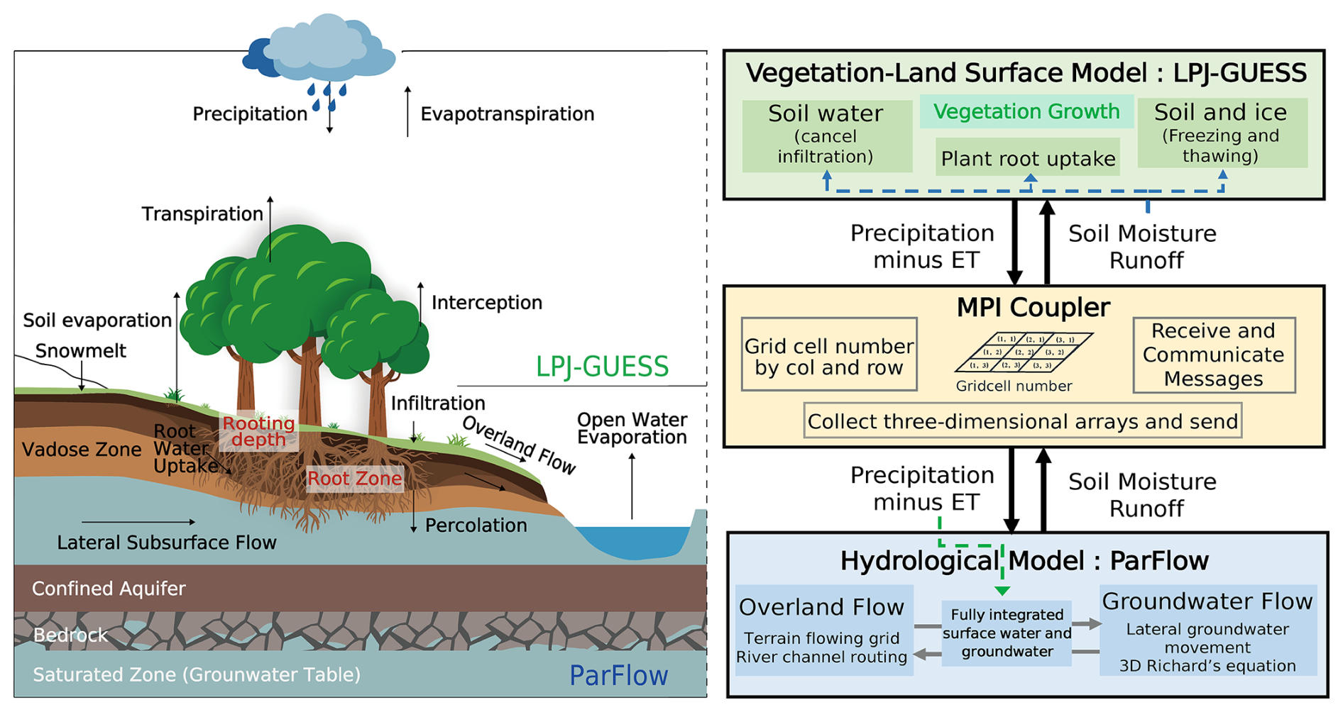
Figure 1Schematic representation of the coupled vegetation dynamics–surface-subsurface flow system. Blue dash arrows indicate outline fluxes calculated and passed by ParFlow, green dash arrows represent net water input (P-ET) computed and passed by LPJ-GUESS.
Several modifications on the LPJ-GUESS structure were made before coupling: (1) the original fixed-depth soil discretization (15 layers at 10 mm each) was replaced with four variable-depth layers with layer thickness of 0.1, 0.3, 0.6, and 1 m, totalling 2 m, to align with the discretized soil columns used by ParFlow; (2) layer-specific soil property inputs (sand, clay, and silt content) were introduced to represent vertical heterogeneity in hydraulic properties; (3) Soil water content simulated by ParFlow was used to overwrite the internal soil moisture states in LPJ-GUESS; (4) an MPI-based coupler was embedded within the main LPJ-GUESS framework (framework.cpp), enabling synchronous, two-way communication between the two models while preserving their native solvers.
The coupling methodology involved replacing the one-dimensional soil moisture and runoff module in LPJ-GUESS with the three-dimensional surface-subsurface flow module in ParFlow. In the coupled model, LPJ-GUESS reads ParFlow outputs every 24 timesteps (1 d) to compute daily water fluxes. These daily P-ET values are disaggregated into hourly values according to diurnal patterns and passed back to ParFlow for the next simulation day. Daily, ParFlow provides LPJ-GUESS with updated soil moisture and surface/subsurface runoff fields. At the same time, LPJ-GUESS returns the net atmospheric water input (precipitation minus evapotranspiration, P-ET) as an upper boundary condition to ParFlow. This two-way exchange ensures a fully interactive and temporally consistent coupling of hydrological and ecological processes.
The interaction occurs in the top soil layers (0–2 m). During the coupled simulation, LPJ-GUESS simulates one patch of a single stand type with the probabilistic patch-destroying disturbance turned off to prevent the complete loss of vegetation from an entire grid cell in a single event. Each patch in LPJ-GUESS aligns with the uppermost layer of a vertical column in ParFlow, ensuring consistency between the soil columns in both models.
2.4 Data sets for model parameterizations and evaluations
The Danube River Basin encompasses both humid and semi-arid regions, with diverse topography from mountains to plains, making it ideal for studying hydrological processes. The basin is also relatively unaffected by intensive human activities, like groundwater pumping and large-scale irrigation, and it has been extensively studies (Naz et al., 2023; Zhou et al., 2024).
2.4.1 Meteorological data
For the Danube River Basin, the ERA5-LAND dataset with a horizontal spatial resolution of 0.1° × 0.1° (∼ 10 km) from 1980 to 2018 served as the meteorological forcing data and is available from the Copernicus Climate Data Store (https://doi.org/10.24381/cds.e2161bac, Muñoz Sabater, 2019). The meteorological data included precipitation, 10 m u-component of wind (east-west), relative humidity, surface downwelling shortwave radiation, surface air pressure, and 2 m temperature, all aggregated to a daily time scale using the CDS (Climate Data Store) daily aggregation method (averages or sums the original hourly ERA5-LAND data to produce consistent daily values while preserving energy and mass balance). To achieve model the long-term hydrological equilibrium, ERA5-Land precipitation and LPJ-GUESS-simulated evapotranspiration was used to create multi-year mean P-ET (1980–2018), applied in the model as regional potential recharge (Fig. S1d in the Supplement).
2.4.2 Soil data
The hydrogeological structure of the coupled model domain consists of shallow soil layers and deeper bedrock units. The top 2 m of model domain is divided into four soil layers with thicknesses of 0.1, 0.3, 0.6, and 1.0 m, from top to bottom. Layer-specific properties including fractions of sand, clay, silt, organic carbon, pH, and bulk density were derived from the WISE database, which integrates data from the FAO Soil Map and the Harmonized World Soil Database (HWSD) (Batjes, 2016). The original 30 arcsec × 30 arcsec (∼1 km) soil grid was resampled to a 10 km resolution using the dominant soil type method. These soil data were aggregated to match the model layers and served as inputs for both ParFlow and LPJ-GUESS to ensure consistency in physical soil representation across the coupled modelling framework (Fig. S2).
2.4.3 Subsurface data
The model uses a three-dimensional indicator array to spatially assign hydrogeological unit properties with all subsurface data resampled to a 10 km resolution to maintain the consistency of the model resolution. Each soil texture or hydro-lithologic class is associated with a representative set of hydraulic parameters, including hydraulic conductivity, porosity, and relative permeability curves. Below the soil, six bedrock layers are discretized with thicknesses of 5, 10, 10, 10, 25, and 50 m from top to bottom, allowing the model to capture both shallow unconfined aquifers and deeper confined aquifers. Hydrogeology categories in the indicator file were reclassified from the permeabilities of GLHYMPS 1.0 dataset (Gleeson et al., 2014), constructed by classifying lithologies from the global lithological map (GLiM) (Fig. S3). These classes were further refined using the hydrogeological map of the Danube River Basin (Duscher et al., 2015).
To better represent actual bedrock conditions, a variable-depth flow barrier was set between each bedrock aquifer, with the reference bedrock depth values from Shangguan et al. (2017) (Fig. S1c). The flow barrier reduces vertical water flux across grid interfaces by a factor of 0.001, enabling the model to distinguish between shallow unconfined aquifers and deep confined aquifers (Tijerina-Kreuzer et al., 2024). Additionally, an e-folding method was applied to the subsurface, which reduces hydraulic conductivity with depth and slope using a depth-dependent factor (Fan et al., 2007). Multiple model configurations were tested to assess the sensitivity of groundwater dynamics to subsurface parameterization. These included variations in the presence of vertical permeability barriers, hydraulic conductivity anisotropy, spatial variability of bedrock classifications. Details of all subsurface parameter values can be found in the Supplement of Maxwell and Condon (2016) (Table S1 in the Supplement).
2.4.4 Land Cover and Manning's n
Land cover classification was derived from the MODIS Land Cover Type product (MCD12Q1, Version 6.1), which provides global coverage at a 500 m spatial resolution (Friedl and Sulla-Menashe, 2022). This classification was derived from the Land Cover Type: The International Geosphere-Biosphere Programme (IGBP) global classification scheme and was resampled to 10 km resolution using the majority method (Foster and Maxwell, 2019) to match the PF-LPJG model resolution (Fig. S1b).
To parameterize spatially variable surface roughness, Manning's n coefficients were assigned based on land cover types, with further adjustments in stream order networks. River channels were delineated using the PriorityFlow algorithm with a threshold drainage area of 50 km2, and stream orders were assigned following the Strahler classification system (Strahler, 1957). Manning's coefficients for streamflow were assigned to decrease with increasing stream order, reflecting reduced channel resistance in higher-order rivers (Gochis et al., 2015).
2.4.5 Topography and rivers
The Digital Elevation Model (DEM) data for the study area were obtained from the MERIT Hydro IHU dataset. MERIT Hydro IHU is a global hydrography dataset upscaled from the 3′′ resolution MERIT Hydro using the Iterative Hydrography Upscaling (IHU) algorithm (Eilander et al., 2021). MERIT Hydro IHU provides multiscale topographic information at spatial resolutions of 30′′ (∼ 1 km), 5′ (∼ 10 km), and 15′ (∼ 30 km). For this study, the 5′ DEM was selected and resampled it to 10 km using the minimum resampling method in QGIS (Zhang et al., 2021; Fig. S1a).
To ensure a fully connected drainage network in the study area, the upscaled DEM and river network was pre-processed with the priority flow algorithm to specify the slope in the x and y directions (Condon and Maxwell, 2019b). This algorithm enforces drainage in the primary east, west, south, and north directions (D4 directions) because the model's hydrological simulations are based on partial differential equations (PDEs) (Zhang et al., 2021). The calculated slope was calibrated based on the drainage area (∼ 10 km) in MERIT Hydro IHU for the Danube River basin and further refined by the parking lot tests to accurately determine river network locations and eliminate anomalous ponding points (Bhaskar, 2010).
2.4.6 Datasets for evaluation
The modelled daily streamflow was compared to river flow observations from the Danube River Basin, obtained from the Global Runoff Data Centre (GRDC, obtained at https://grdc.bafg.de/, last access: 21 August 2025). The simulated surface SM at 0.1 m depth was evaluated by comparison with the global satellite-based estimates from the European Space Agency Climate Change Initiative Soil Moisture product, ensuring that NaN values in the original data were excluded from the correlation calculation (ESA CCI-SM; Dorigo et al., 2017). To match the model-simulated SM with the dataset, we interpolated the ESA CCI-SM data from 0.25° to 0.1° (∼ 10 km) resolution using bilinear interpolation. The validation of ET data was performed using Global Land Evaporation Amsterdam Model (GLEAM) 4.2 datasets, which employ the Priestley-Taylor equation and other algorithms to estimate ET separately for both soil and vegetation (Miralles et al., 2025). Both GLEAM4 and ESA CCI-SM provide long-term, globally coverage datasets with relatively high spatial resolution, are extensively used as reference products for the validation of hydrological, climatic, and land surface models.
2.5 The modelling spin-up
The PF-LPJG coupled model was simulated over the Danube River Basin with a horizontal resolution of 10 km, resulting in a grid of 161 columns × 82 rows. The model total depth is 112 m below the surface (depends on the bedrock depth on Danube basin) and consists of 10 layers with variable thicknesses of 50, 25, 10, 10, 10, 5, 1, 0.6, 0.3, and 0.1 m from bottom to top, capturing the transition from shallow soil to deep aquifer systems. No-flow boundary conditions were prescribed along the lateral and bottom boundaries, while the upper boundary employed a kinematic wave formulation to simulate overland flow processes.
To ensure a physically consistent initial condition, a two-phase spin-up was adopted for the coupled system. First, ParFlow and LPJ-GUESS were spun up independently. For ParFlow, the model was initialized using the long-term (1980–2018) average net water input (P-ET), with the ET derived from multi-year average LPJ-GUESS simulations over the Danube River Basin. The initial groundwater table was set at a depth of 5 m, removing all positive pressure heads and prohibiting overland flow. The model runs until the change in groundwater storage stabilizes, with fluctuations less than 1 % of the potential recharge (P-ET), allowing the subsurface system to reach equilibrium over the spin-up period (Seck et al., 2015; Ajami et al., 2014). In the second phase, overland flow was activated, and ParFlow was run for a prolonged duration to allow the coupled surface-subsurface flow system to reach hydrological steady state (the total storage change was less than 3 % of the P-ET) and generate a stable stream network structure. For LPJ-GUESS, a 500 year spin-up process using repeated 30 year meteorological forcing (1980–2010) was used to estimate vegetation composition and biomass at dynamic equilibrium in response to climatic and edaphic conditions. Soil organic matter is additionally spun-up offline at year 300 of the standard LPJ-GUESS spin-up for 40 000 years using repeated 100 year soil moisture and temperature status and litter input from years 200–300.
Following the individual spin-ups with saved state variables, the fully coupled PF-LPJG model was initialized and driven by repeating the meteorological data of 1980 for 10 consecutive years to reach dynamic equilibrium of the two models before starting the formal simulation (1980–2018). The spin-up period precedes significant human activities such as dam construction, hydroelectric power plants, and groundwater pumping in the modelling domain.
2.6 Model evaluation
To systematically evaluate the performance of the coupled model PF-LPJG in streamflow simulation, we use four statistical metrics between observed and simulated values: Spearman rank correlation coefficient (to assess the model's ability to capture streamflow trends), Kling-Gupta Efficiency (KGE, to evaluate holistic model behaviour), Percent Bias (PBIAS, to reflect systematic bias), and Root Mean Square Error-observations Standard deviation Ratio (RSR, to assess relative error). These metrics were selected to provide a comprehensive assessment of the model's performance against in situ, remote sensing observations, and reanalysis datasets, assessing both the accuracy of the simulated values and their temporal and spatial dynamics.
Spearman's ρ is a non-parametric measure of monotonic association between two variables.
Where di is the difference between the ranks of observed and simulated values for the observation, n is the total number of values.
KGE explicitly decomposes model performance into correlation, bias, and variability components to evaluate the strengths and weaknesses of the model.
Where r is the Pearson correlation coefficient between observed and simulated values, β and γ are the bias ratio and variability ratio.
PBIAS measures the average tendency of the simulated values to be larger or smaller than their observed counterparts.
Where si is simulated value at time i, oi is observed value at time i.
RSR is the ratio of the root mean square error (RMSE) to the standard deviation of the observed data.
Where σo is the standard deviation of observed values, i is the total number of observations.
3.1 Evaluation of streamflow
This section assesses the model's ability to reproduce observed hydrological behaviour across seven GRDC stations representative of diverse catchment sizes (large, medium, small) and climatic conditions in the Danube basin. These stations were selected based on their spatial representativeness in terms of geographic distribution and catchment characteristics, and the availability of complete daily discharge data for the period 1980–2018. The PF-LPJG coupled model, by explicitly coupling LPJ-GUESS with a physically based groundwater module via ParFlow, offers substantial improvements in capturing streamflow dynamics compared to its uncoupled counterpart. As shown in the boxplots of performance metrics for the seven basins, the PF-LPJG model systematically outperforms the stand-alone LPJ-GUESS model across all key metrics, with higher trend consistency and correlation, and lower bias and relative error (Fig. 2). Notably, over 80 % of the gauging stations report KGE values exceeding 0.5 and Spearman coefficients above 0.8, demonstrating the coupled model reliably captures the temporal consistency and responds to hydrological variability (Fig. 3). The improvements seen in PF-LPJG are particularly salient at major downstream locations (e.g., CEATAL IZMAIL), where all performance metrics demonstrate clear enhancement.
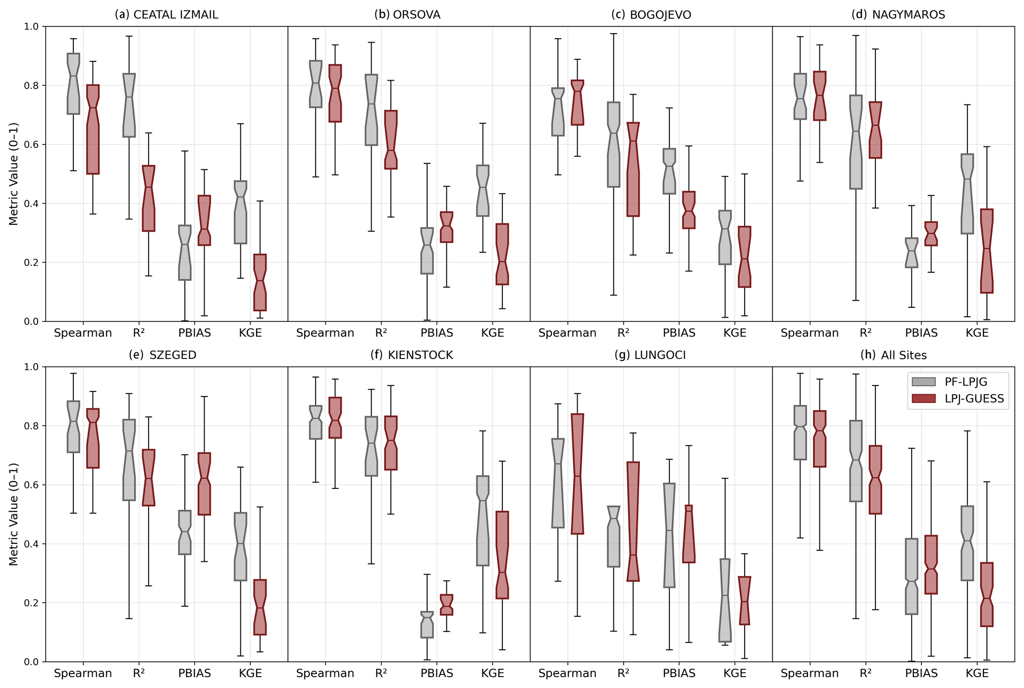
Figure 2Boxplots of performance metrics (Spearman coefficient, R2, PBIAS, RSR, and KGE) for daily streamflow simulated by PF-LPJG and LPJ-GUESS against GRDC observations.
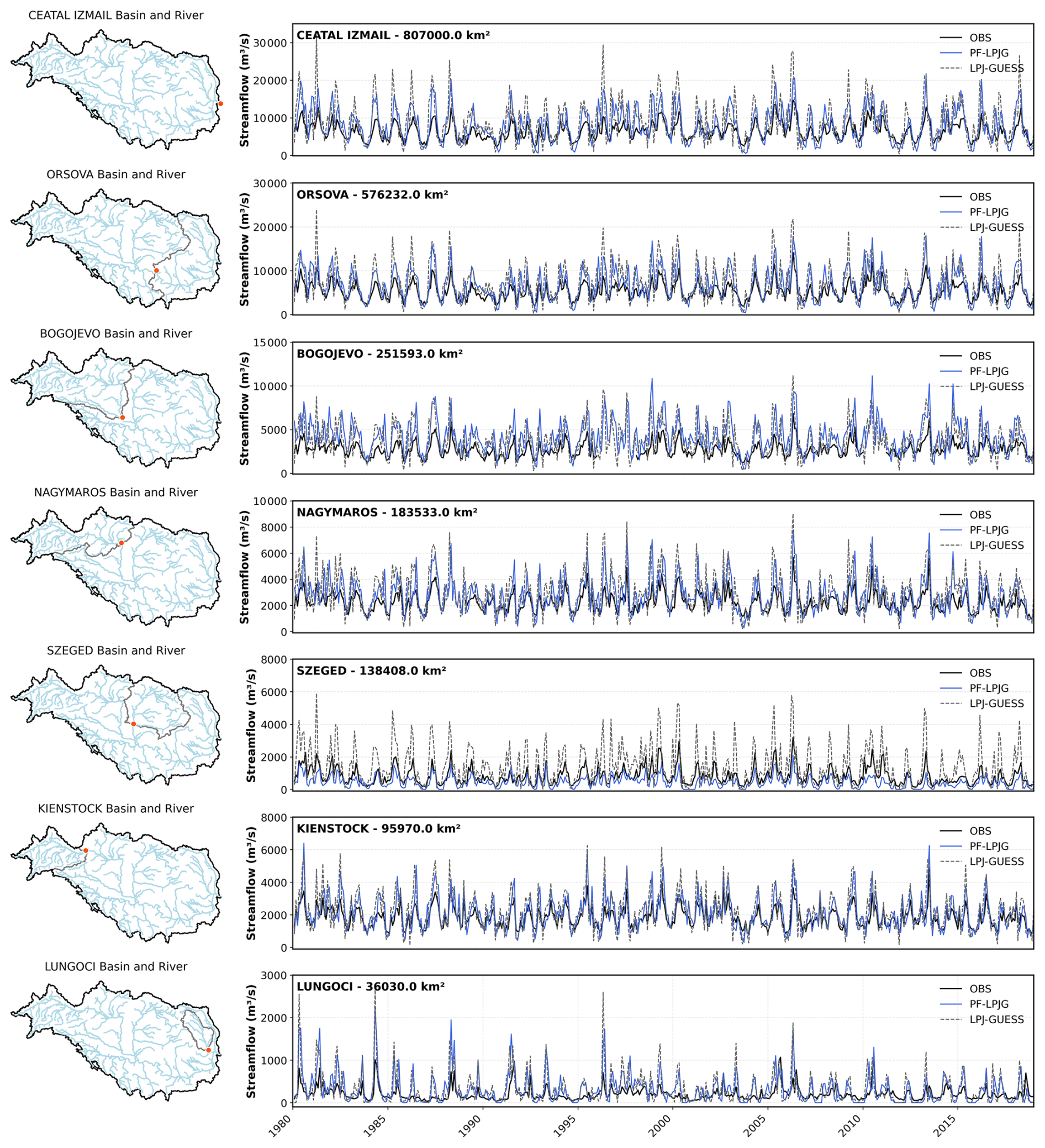
Figure 3Comparison of monthly discharge simulated by the coupled model PF-LPJG and the stand-alone LPJ-GUESS at seven gauging stations from the GRDC dataset.
Despite these improvements, both PF-LPJG and LPJ-GUESS exhibit limitations under hydroclimatic extremes (wet year: P-ET above the long-term mean; dry year: P-ET below the long-term mean). During anomalously wet years (e.g., 2010, 2014), both PF-LPJG and LPJ-GUESS overestimate peak flows and underestimate low flows during dry years (e.g., 2003, 2011). Nevertheless, PF-LPJG exhibits a substantially narrower bias range (PBIAS: 0.2–0.4) and improves relative error metrics (RSR: 0.9–1.3), compared to LPJ-GUESS (PBIAS: 0.3–0.5; RSR: 1.7–2.0) (Fig. 2), suggesting that coupled groundwater dynamics contribute to more stable and physically consistent responses.
The PF-LPJG model exhibits strong seasonality in performance, with higher consistency during spring snowmelt and summer rainfall-driven peaks. In dry years (1983, 1987, 2003, 2006, and 2015), more than four gauging stations, including upstream and downstream locations (CEATAL IZMAIL, ORSOVA, SZEGED, KIENSTOCK), show both R2 and Spearman's ρ > 0.9, and KGE > 0.5. This consistency indicates improved simulation of seasonal runoff processes across the basin. Conversely, the model's skill deteriorates in the year 2001, with the weakest model performance across the basin (R2 and Spearman's ρ are: 0.1–0.3; KGE ≈ 0 at multiple stations). Although the year 2001 did not rank among the extremes of precipitation, temperature, or ET, its poor performance may reflect lagged hydrological effects from 2000, a dry year with the third lowest P-ET value. This likely reflects disrupted hydrological connectivity between soil moisture and active surface water components (Good et al., 2015), underscoring the need for improved parameterizations and potential assimilation of satellite-derived soil moisture and groundwater storage data (Clark et al., 2015).
From a spatial perspective, PF-LPJG performs better in medium-to-large catchments (> 10 000 km2), where hydrological signals are less sensitive to local-scale heterogeneity. Conversely, smaller basins (e.g., LUNGOCI) exhibit poor simulation performance (KGE = 0.046; PBIAS = 49.1 %) (Fig. 3), likely due to coarse spatial resolution (10 km), unresolved anthropogenic influences (e.g., reservoirs, pumping), and scaling issues inherent in DGVMs (Wood et al., 2011). Building high-resolution routing schemes or regional hydrological models could mitigate such deficiencies.
In summary, the PF-LPJG model represents a notable advancement in large-scale land surface hydrology by embedding groundwater–surface water interactions into a DGVM. This integration allows for improved representation of both mean flow conditions and hydrological extremes, even without empirical calibration or high-resolution.
3.2 Evaluation of Evapotranspiration
Figure 4a–f presents the spatial distribution of mean annual ET for the period 1980–2018 from PF-LPJG, LPJ-GUESS, and GLEAM, along with their inter-model differences. PF-LPJG successfully reproduces the similar spatial patterns of ET across the basin, capturing gradients from the drier western and northeastern regions to the wetter central zones. However, the model tends to underestimate ET in colder northern and southwestern regions (where the mean annual temperature is < 0 °C) and overestimate ET in the humid central lowlands. These biases are consistent with prior studies using ParFlow in Europe (Naz et al., 2023), where ET discrepancies in river channels were primarily due to ParFlow's default assumption that soil saturation is set to 1.0 in river channel cells.
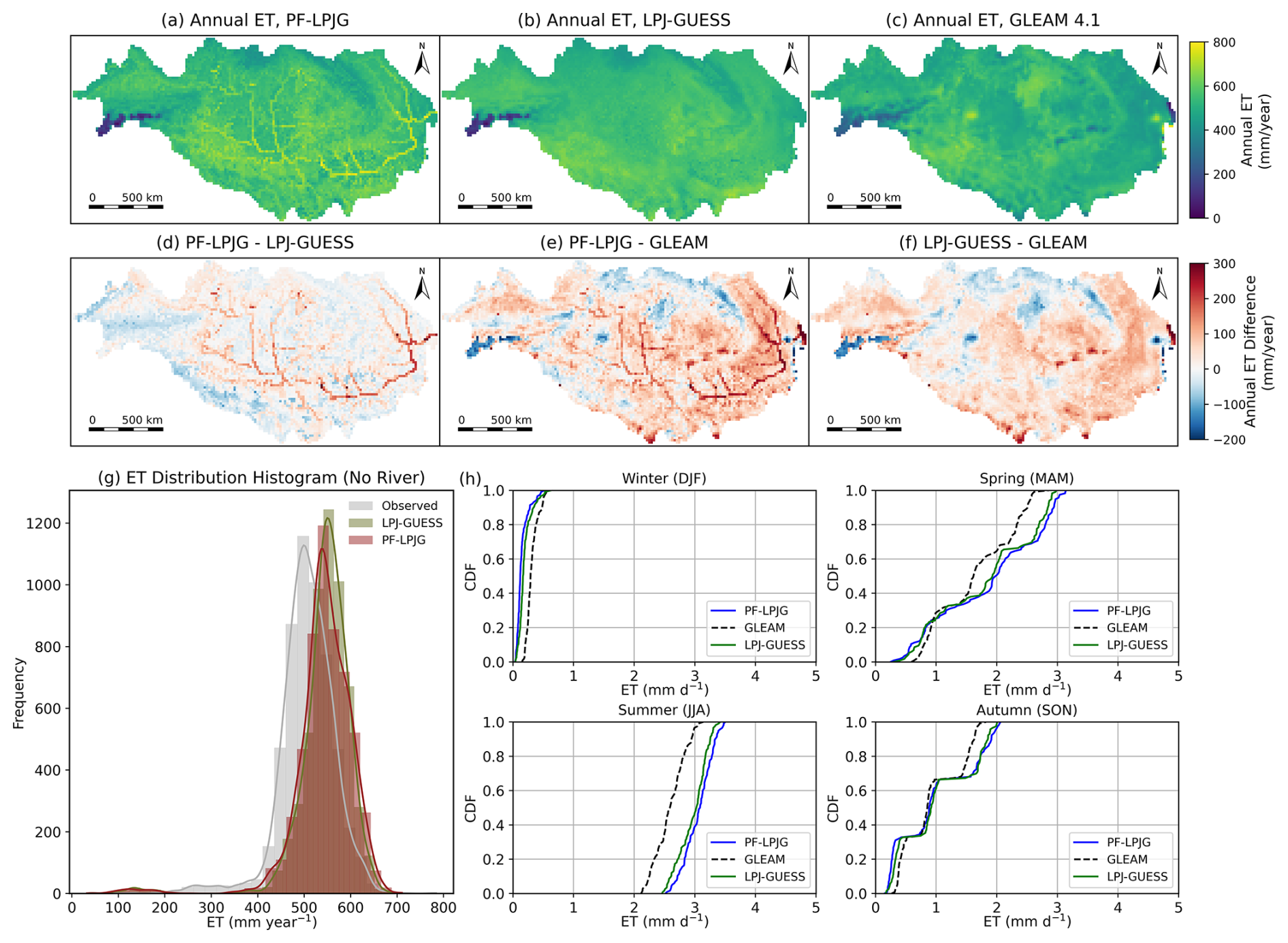
Figure 4Spatial distribution of mean annual ET (a–c) and inter-model differences (d–f) for the period 1980–2018 as simulated by the coupled model PF-LPJG, the stand-alone model LPJ-GUESS, and the GLEAM 4.2 datasets across the Danube River Basin. (g) Histogram of mean annual ET from GLEAM v4.2, LPJ-GUESS, and PF-LPJG. (h) Cumulative distribution function (CDF) comparison of seasonal (DJF, MAM, JJA, SON) ET comparing PF-LPJG and GLEAM v4.2a.
We further analysed monthly ET outputs from PF-LPJG and LPJ-GUESS. Across most of the Danube basin, differences between the two models are small (mean bias: −0.007 mm d−). The PF-LPJG model shows a slight improvement in agreement with GLEAM data when river-channel grid cells are excluded from the analysis. Specifically, the mean difference between PF-LPJG and GLEAM (0.101 mm d−) is marginally smaller than that of LPJ-GUESS (0.108 mm d−), suggesting a modest enhancement in ET realism following hydrological coupling (Fig. 4g).
The model's performance in simulating seasonal ET dynamics was evaluated using cumulative distribution functions (CDFs) (Fig. 4h). The seasonal discrepancies between simulated and observed ET vary notably throughout the year. PF-LPJG reproduces a seasonal variability comparable to that of LPJ-GUESS and preserves the seasonal transpiration patterns. During autumn (SON) and winter (DJF), mean ET deviations are relatively minor (0.045 and −0.163 mm d−, respectively), indicating reasonable agreement with GLEAM data. However, during spring (MAM) and summer (JJA), larger positive deviations emerge, with mean differences of 0.226 and 0.464 mm d−, respectively. These summer overestimations are most prominent along the riparian zones of the river network, which may be attributed to increased soil moisture availability and elevated temperatures, both of which promote enhanced ET (Fig. 4h).
3.3 Evaluation of Soil Moisture
To evaluate the performance of the PF-LPJG model in simulating soil moisture dynamics, we compared the simulated volumetric soil water content at 0.1 m depth with satellite-based estimates from the ESA Climate Change Initiative Soil Moisture product (CCI-SM; Dorigo et al., 2017).
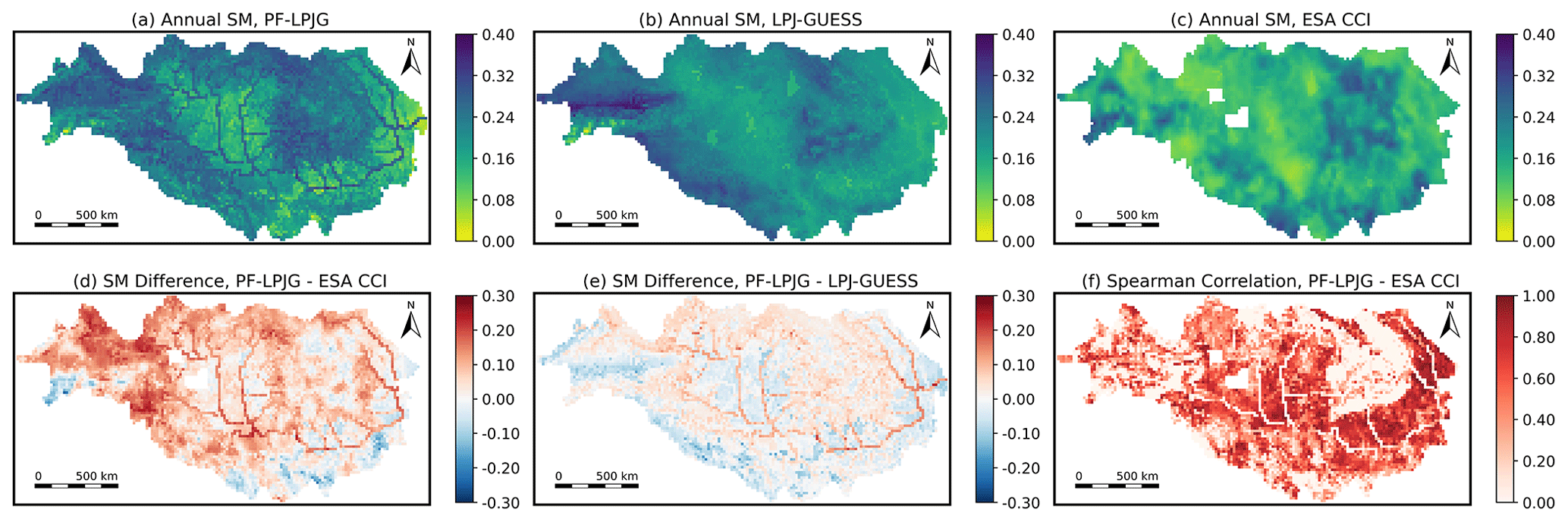
Figure 5(a–c) Time-averaged surface soil moisture (SM) simulated by the coupled model PF-LPJG and stand-alone LPJ-GUESS against the ESA CCI-SM dataset during 1980–2018. (d, e) Mean difference in SM between PF-LPJG and ESA CCI-SM and between PF-LPJG and LPJ-GUESS, respectively. (f) Spearman's correlation in SM between PF-LPJG and ESA CCI-SM.
Figure 5a–c illustrate the spatial pattern of surface volumetric soil moisture simulated by PF-LPJG and stand-alone LPJ-GUESS compare to CCI-SM observations. In humid regions of the Danube Basin, PF-LPJG tends to overestimate near-surface soil moisture, especially during wet months (Fig. 5d and e). This overestimation may be attributed to ParFlow's simulation of lateral and vertical redistribution processes, which enhances surface saturation, particularly in low-relief areas or near river networks (Maxwell and Condon, 2016). The PF-LPJG model captured spatial heterogeneity effectively, owing to its ability to simulate deeper infiltration and slower recharge processes that dominate soil moisture dynamics in water-limited settings. These features enabled PF-LPJG to better simulate deeper soil moisture in arid regions, as indicated by higher spatial correlation with CCI-SM (Fig. 5f).
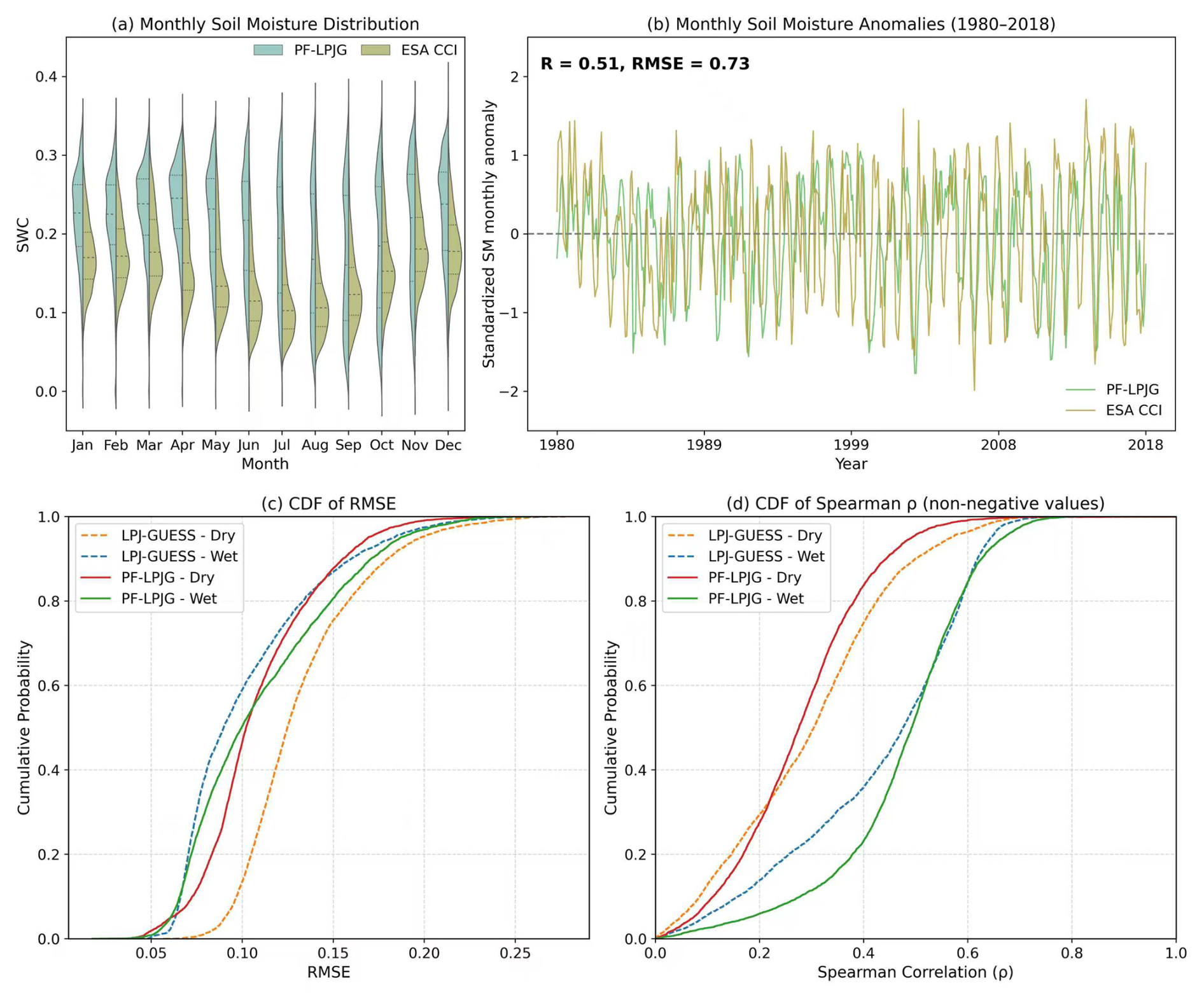
Figure 6(a) Violin plots of the spatial distribution of time-averaged surface soil moisture (SM) from PF-LPJG and ESA CCI-SM over the Danube River Basin during 1980–2018. (b) Spatially aggregated monthly anomalies of surface SM from PF-LPJG and ESA CCI-SM. (c, d) Cumulative distribution functions (CDFs) of RMSE and Spearman's ρ for surface SM in wet (4–9) and dry months (1–3, 10–12), comparing PF-LPJG and LPJ-GUESS simulations against ESA CCI-SM.
The Violin plots comparing monthly soil moisture distributions between PF-LPJG and CCI-SM show that PF-LPJG generally overestimates soil moisture, particularly in wet months (Figs. 6a and S4). Monthly anomalies of surface soil moisture aggregated across the Danube Basin over the period 1980–2018 are shown in Fig. 6b. The PF-LPJG exhibits good temporal consistency with CCI-SM anomalies (Spearman's ρ = 0.51, RMSE = 0.73 cm3 cm−3), indicating an improved capacity to capture both seasonal and interannual variability. Anomalously low soil moisture anomalies in early 1985 simulated by PF-LPJG were likely caused by extremely low temperatures in January and February of that year, with mean basin-wide temperatures below 0 °C. These conditions resulted in widespread snow accumulation, reduced meltwater availability, and suppressed evapotranspiration. These cold-season hydrological effects are consistent with previous findings on snow-dominated basins (Ionita et al., 2018). All of which were reflected in the PF-LPJG simulation.
Model performance under hydroclimatic extremes was further evaluated by analysing cumulative distribution functions (CDFs) of RMSE and Spearman correlation coefficient values for dry and wet months from 1980 to 2018 across the Danube River basin (Fig. 6c and d). The results indicate that PF-LPJG significantly improved soil moisture simulation during dry periods, with higher correlation and lower error compared to LPJ-GUESS (Figs. 6c, d and S5). This enhancement is attributed to the representation of soil–groundwater feedbacks, including infiltration and subsurface storage buffering, which are largely absent in traditional DGVMs (Fan et al., 2019). During drought events, PF-LPJG exhibits stronger vertical flux dynamics and a clearer depletion signal in surface soil moisture, more closely aligned with CCI-SM anomalies. Additionally, the dynamic interaction between vegetation available water and root-zone uptake water reinforces the model's responsiveness to water stress, as vegetation dynamics directly affect soil moisture redistribution and evapotranspiration efficiency (Bonan, 2019; Fan et al., 2017). However, its advantage is less evident under wet conditions. This may be attributed to the reduced role of subsurface processes when soils are near saturation, limiting the contribution of explicit groundwater representation.
At the spatial scale, PF-LPJG effectively captures heterogeneity in soil moisture, benefiting from ParFlow's three-dimensional representation of groundwater flow and topographic controls (Kuffour et al., 2020). In the northwestern basin, where annual precipitation exceeds evapotranspiration, elevated groundwater tables result in persistent surface saturation and slight overestimations of soil moisture. Nevertheless, high spatial correlation with CCI-SM, particularly under water-limited conditions, indicates that PF-LPJG realistically simulates the dominant controls on soil water dynamics across diverse hydroclimatic gradients (Soltani et al., 2022).
As a whole, PF-LPJG captures both short-term soil moisture variability and the legacy effects of wet or dry conditions, providing strong seasonal and interannual memory in soil moisture.
3.4 Evaluation of Water Table Depth
To evaluate the ability of the PF-LPJG model to simulate groundwater dynamics, we compared modelled WTD outputs (annual mean WTD) against two independent datasets: (1) a global gridded WTD benchmark produced by Fan et al. (2013), and (2) in-situ groundwater observations from monitoring wells across the Danube Basin (Fan et al., 2013). As shown in Fig. 7a, the PF-LPJG model achieved a residual-based RSR (RMSE divided by the standard deviation of observations) of 1.31, which is substantially lower than the RSR of 4.46 from the Fan et al. simulation. The histogram of the absolute errors between PF-LPJG and observational data (Fig. 7b) indicates that for most well points (48 observation points), the difference between the simulated WTD value and the observed WTD value is within the 0–5 m range. The evaluation shows that the PF-LPJG model performs well in reproducing observed WTD dynamics.
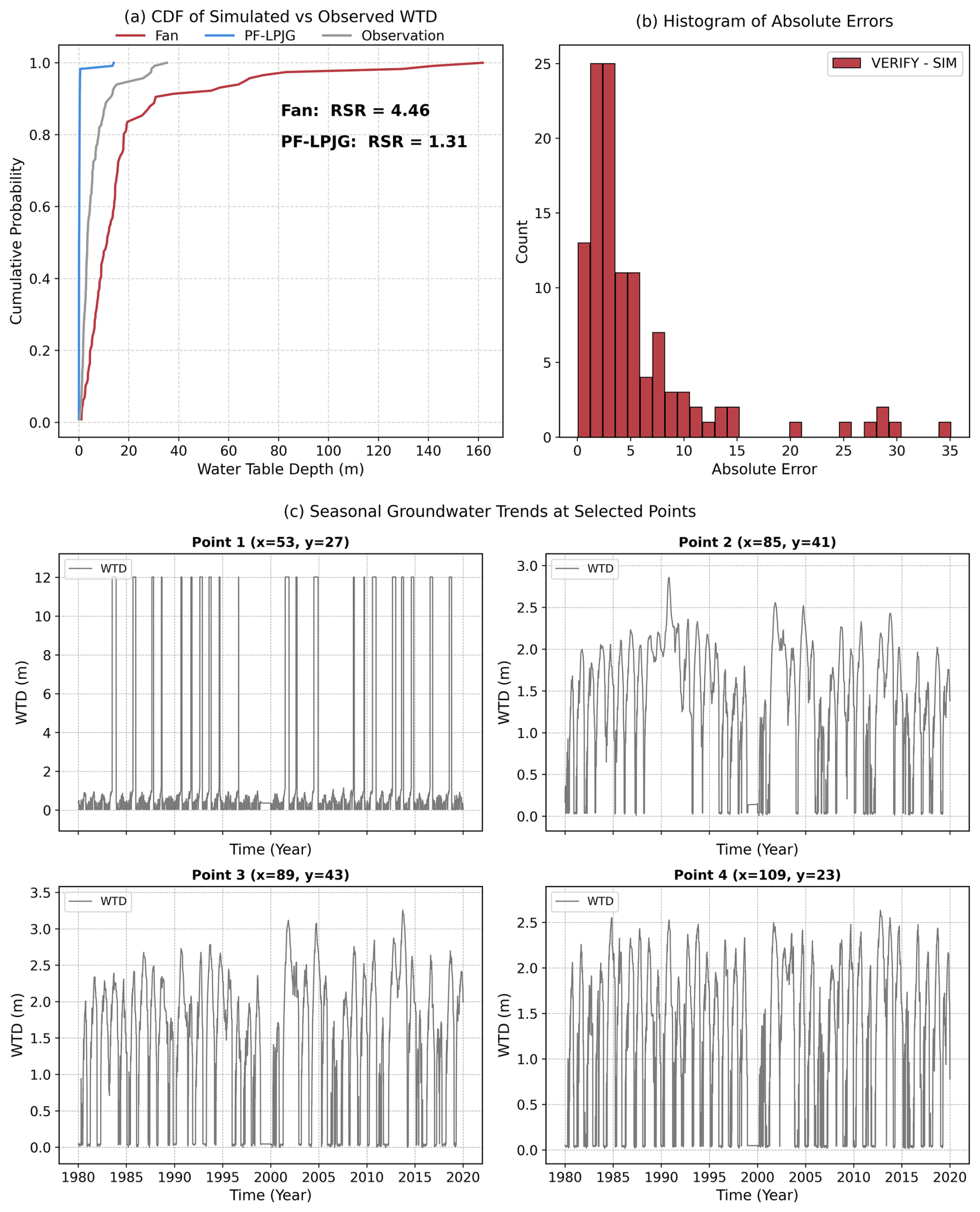
Figure 7(a) Cumulative distribution function (CDF) of WTD as simulated by PF-LPJG and Fan's model with observed WTD data. (b) Histogram plots of the absolute errors between PF-LPJG simulated minus observed WTD. (c) Monthly mean time series of simulated WTD by PF-LPJG at selected monitoring sites.
In addition, the cumulative distribution functions (CDFs) of WTD from monitoring stations revealed that PF-LPJG better captured the range of water table fluctuations, particularly in regions with deeper water tables. All 48 in-situ wells are located in the lower reaches of the Danube River, where groundwater depths typically range from 0 to 40 m. In this area, soil moisture oversaturation leads PF-LPJG to simulate very shallow water table depths (≈ 0–1 m) at certain locations. In regions with relative deeper groundwater, the modelled WTD ranges from 0 to 20 m, showing substantially better agreement with observational data than the Fan et al. (2013) dataset, which systematically overestimates WTD (typically exceeding 40 m) in these lowland environments. Overall, PF-LPJG more accurately reproduces both the magnitude and spatial variability of groundwater depths across the basin.
Figure 7c illustrates the monthly mean time series of WTD simulated by PF-LPJG at selected monitoring sites. At sites where WTD exhibited low interannual variability and smooth transitions, the model effectively replicated this stability, suggesting that PF-LPJG can reproduce both dynamic and quasi-steady groundwater regimes (Fig. 7c). Furthermore, seasonal groundwater dynamics were well captured, with water tables rising in response to spring and summer recharge (typically peaking in September) and gradually declining through the dry winter months (Fig. S6).
3.5 Discussion
3.6 Improvement of Evapotranspiration Partitioning
To disentangle the hydrological controls on (ET), we decomposed ET into bare-soil evaporation (E) and plant transpiration (T). While E is predominantly determined by near-surface soil moisture availability, T reflects root-zone water uptake and is modulated by vegetation phenology and physiological traits (Maxwell and Condon, 2016; Li et al., 2019). To assess the role of groundwater in regulating the partitioning between E and T, we compared monthly cumulative values of T, E (Fig. 8a), and their ratio () from three data sources (Fig. 8b): the coupled PF-LPJG model, the standalone LPJ-GUESS model, and the GLEAM v4.2 dataset.
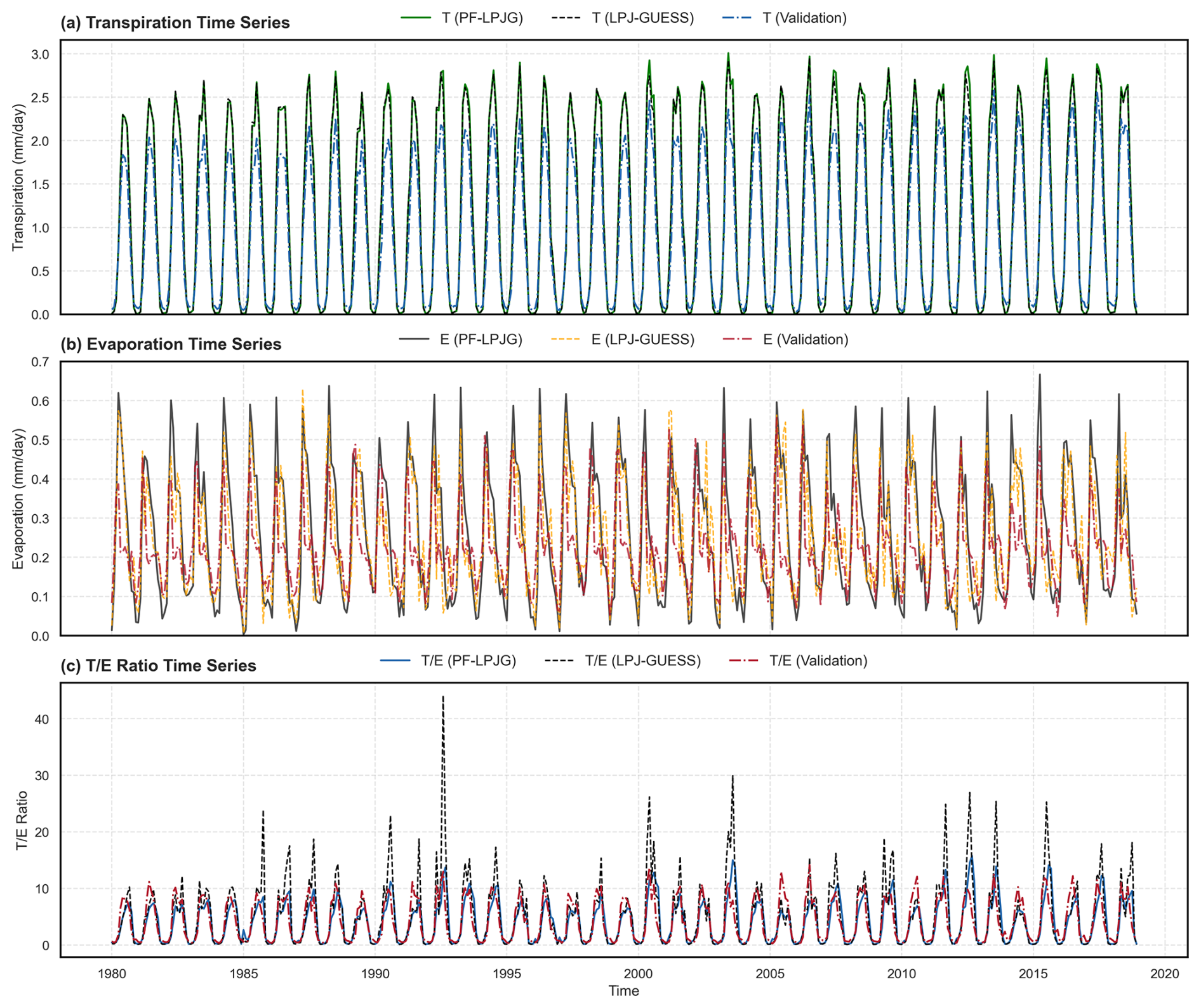
Figure 8Monthly cumulative values of transpiration (T) and evaporation (E) (a), and the ratio () (b) as simulated by the coupled model PF-LPJG, the stand-alone model LPJ-GUESS, and the GLEAM v4.2 dataset.
The results reveal that PF-LPJG captures the seasonal dynamics of with higher fidelity to GLEAM, especially during summer months characterized by elevated atmospheric evaporative demand (Fig. 8). In contrast, LPJ-GUESS exhibits unrealistic peaks and severely constrained E during these periods, indicative of a rapid depletion of shallow soil moisture in the absence of upward capillary fluxes from the groundwater table, limiting E and leading to unstable ratios.
The incorporation of a physically based groundwater component in PF-LPJG enhances surface moisture supply which in turn improves plant water utilization during dry or hot periods, thereby supporting bare-soil evaporation and stabilizing the ratio (Fig. 8b). Although T remains relatively constant across simulations, small increases in evaporation enabled by groundwater can significantly lower the ratio, highlighting the groundwater contributions can noticeably shift the balance of ET partitioning. This behaviour reflects the groundwater dependence of the ET partitioning process, as previously observed in empirical studies (Condon et al., 2020; O'Connor et al., 2019; Davison et al., 2018). The agreement with seasonal dynamics between PF-LPJG estimates and GLEAM reinforces the hypothesis that subsurface-plant hydrological connectivity plays a critical role in mediating the E-T partitioning, particularly under climatic extremes.
Nonetheless, limitations remain in the model representation. The use of a fixed rooting depth (0–2 m) and a static exponential root distribution (controlled by PFT specific parameter, Root_Beta) in LPJ-GUESS does not account for root plasticity in response to vertical soil moisture gradients or fluctuating groundwater levels. Such simplifications constrain the model's ability to represent vegetation strategies under water stress, especially for deep-rooted species and phreatophytes (Feddes et al., 2001; Warren et al., 2015). Future work may incorporate dynamic root modelling to allow root distribution to respond to variations in soil water availability (Lu et al., 2019).
3.7 Model Strengths and Performance
The advancement of streamflow simulation reflects the well-documented limitation in the current dynamic vegetation models (DGVMs), which typically exhibit poor streamflow simulation performance when groundwater dynamics and lateral flow processes are inadequately represented (Yang et al., 2015; Hong et al., 2025). By integrating subsurface hydrological processes, PF-LPJG addresses a long-standing limitation in ecohydrological modelling (Guillaumot et al., 2022). More specially, these improvements stem from the integrated, physically based groundwater–surface water interactions enabled by ParFlow. Unlike empirical routing schemes, the coupling model resolves the expansion and contraction of surface water channels purely from flux balances and terrain properties, without requiring any a priori specification of inundated areas (i.e., rivers, lakes, and wetlands). This is consistent with other advanced models such as CLM-ParFlow and mHM-HGS, which have shown similar strengths in capturing low-flow dynamics and recession curve representation (Maxwell and Miller, 2005; Kumar et al., 2013).
Fundamentally, the PF-LPJG coupling formulates terrestrial hydrology as a dynamic boundary-value problem in which both upper (P-ET) and lower (subsurface water) boundaries evolve interactively. This enables emergent nonlinear feedbacks between vegetation dynamics (e.g., stomatal regulation, rooting strategy) and subsurface hydrology-feedbacks that are not represented in traditional land–surface models. Such process-based coupling provides a more realistic representation of vegetation-water interactions across diverse climates, strengthens the physical consistency of water-carbon interactions and provides a pathway toward more realistic representations of terrestrial processes in Earth System Models.
The model's ability to mitigate summer low-flow underestimation during dry years and to better capture peak timing in wet years demonstrates the role of groundwater buffering. These improvements reflect that groundwater contributions can help delay soil moisture depletion, maintain streamflow, and support plant growth demand under drought conditions. Especially, subsurface water stores wet-season infiltration and routes it to streams during dry periods, resulting in a fairly constant baseflow year-round and sustaining summer discharge a process poorly represented in conventional DGVMs (Berghuijs et al., 2024; Condon and Maxwell, 2019a). Although some positive ET biases remain near river channels due to ParFlow's tendency to saturate riparian zones, PF-LPJG overall shows improved spatial and seasonal ET patterns relative to stand-alone LPJ-GUESS (Fig. 4e, g, and h). These improvements are evident across a range of hydroclimatic settings within the Danube basin and highlight the benefits of integrating physically based hydrological processes into terrestrial ecohydrological models.
Notably, in the low-gradient regions of the Danube Basin, soil moisture preferentially accumulates in depressions, leading to modelled evapotranspiration values near river channels that exceed the estimates provided by GLEAM. This discrepancy arises because PF-LPJG simulates enhanced soil moisture accumulation in topographically low areas as a result of lateral groundwater convergence and recharge, a process that is largely absent in the reference products. The PF-LPJG model explicitly resolves the river network and prescribes full soil saturation (i.e., saturation = 1) in river grid cells, whereas the GLEAM v4.2 global product, despite including water body evapotranspiration, because of coarse land cover and river masks, leading to an underrepresentation of narrow river channels and riparian zones. Moreover, PF-LPJG directly solves Richards' equation and groundwater flow, allowing evapotranspiration to be sustained by capillary rise and lateral groundwater redistribution. In contrast, stand-alone LPJ-GUESS lacks groundwater process, which limits its ability to represent drought buffering and baseflow-supported vegetation water use.
Importantly, it should be noted that the datasets used as references for evaluating evapotranspiration and soil moisture (e.g., GLEAM v4.2 and ESA CCI), extensively validated against in-situ measurements and independent datasets, and provide a reasonably reliable benchmark for large-scale hydrological assessments, but are not direct observations but model or retrieval-based products that rely on simplifying assumptions and indirect inference. As such, discrepancies between PF-LPJG and these reference datasets do not necessarily indicate model deficiencies, but may instead reflect differences in process representation, spatial resolution, and data constraints.
This highlights the advantage of PF-LPJG to simulate low-flow dynamics, drought buffering, and baseflow-supported vegetation growth relative to stand-alone LPJ-GUESS model. The results underscore the potential of PF-LPJG as a tool for integrated assessments of land–atmosphere feedbacks and water use dynamics, especially under scenarios of increasing climate variability.
3.8 Model Limitations and Perspectives for Future Development
Despite these advances, we also acknowledge several limitations of this study, persistent peak-flow overestimations in some regions remain, largely due to the limitations of coarse spatial resolution. The 10 km resolution grid leads to a smoothing of topographic gradients, which flattens slopes, shortens flow pathways, and raises groundwater heads, ultimately resulting in unrealistically rapid and voluminous runoff responses. Furthermore, the Danube River basin's cold-climate characteristics, such as suppressed evapotranspiration and intense spring snowmelt, contribute to seasonal runoff amplification (Zhou et al., 2024). This hydrological signature further exacerbates peak overestimation, particularly when land surface energy partitioning is poorly resolved.
Further analysis highlights, the PF-LPJG model appears particularly sensitive to soil texture and hydraulic resistance under dry conditions. In arid regions of the western and northeastern basin, ET rates are lower and closely aligned with GLEAM estimates, indicating that water availability limits evapotranspiration. In contrast, certain flat areas with coarse soils exhibit enhanced ET in PF-LPJG, likely due to increased infiltration capacity and accumulation of shallow soil moisture, which amplifies bare-soil evaporation (Miguez-Macho and Fan, 2012). This effect is exacerbated by the model's spatial resolution (∼ 10 km), which smooths topographic gradients and can lead to artificial surface saturation and restricted drainage in low-slope areas (Jefferson and Maxwell, 2015).
WTD is a critical hydrological variable that governs plant–groundwater interactions, particularly under conditions of water limitation and hypoxia (Fan et al., 2017; O'Connor et al., 2019). It plays a dual role-acting as supplementary water source that sustains transpiration during dry periods, and influencing plant productivity and community composition across diverse climatic regimes. Beyond its ecohydrological relevance, WTD provides a stringent diagnostic for evaluating groundwater model performance due to its spatial and temporal sensitivity to hydrological forcing (Yang et al., 2023).
However, terrain driven oversaturation drives simulated water table depths toward zero at some locations, contributing to discrepancies with observations, particularly in shallow wells (Yang et al., 2025). Additionally, despite PF-LPJG couples groundwater dynamics with land surface processes, vegetation is represented using simplified root water uptake schemes, which constrain the simulation of dynamic root growth-particularly in semi-arid regions where plant water stress largely governs evapotranspiration variability.
To address these limitations, potential avenues for improving the coupled model include: (1) incorporating dynamic vegetation processes, such as variable rooting depth and stomatal regulation, to better capture ET responses under water stress; (2) refining hydrogeological parameters through site-specific calibration using observed water table depths, river discharge, and soil moisture; (3) increasing river network resolution to improve water body representation and reduce grid misclassification; and (4) conducting sensitivity analyses across diverse climatic and topographic regions to inform targeted parameter adjustments, thereby enhancing model performance under different hydrological conditions. (5) revisiting the assumed hydraulic conductivity anisotropy, the model currently assumes hydraulic conductivity anisotropy, with (where Kz includes flow barriers, typically set to 0.01 × Kx, Ky). We plan to increase Kx andKy to better represent groundwater depth in flat and lowland areas. With regard to the running efficiency of the coupled model, both ParFlow and LPJ-GUESS support large-scale parallelization, future work will leverage GPU-accelerated ParFlow, which is expected to increase computational efficiency by a factor of 2–3 for simulations.
This study introduces the first basin-scale, long-term implementation of the fully coupled PF-LPJG modelling framework, which physically integrates the three-dimensional ParFlow hydrological model with the LPJ-GUESS dynamic vegetation model across the Danube Basin at 10 km spatial resolution. We rigorously evaluated the model using comprehensive statistical metrics (KGE, Spearman's ρ, PBIAS, RSR, R2), benchmarking performance against the stand-alone LPJ-GUESS model, and further evaluated against different observational datasets. The PF-LPJG framework demonstrated substantial improvements in runoff and soil moisture simulations compared to standalone LPJ-GUESS. The coupled model achieved strong performance (R > 0.8 and KGE > 0.5) without parameter calibration at four out of seven gauging stations, including both headwater and outlet sites, with particularly remarkable improvements at basin outlets. These enhancements highlight the role of the ParFlow variably saturated flow solver in enhancing lateral subsurface redistribution and drainage processes-critical mechanisms for large-scale hydrological and ecosystem modelling. Moreover, PF-LPJG also improved the partitioning of evapotranspiration. The simulated transpiration-to-evaporation () ratios aligned more closely with observations from the GLEAM v4.2 dataset. These improvements reflect the model's capacity to sustain evapotranspiration under hydroclimatic stress through capillary rise and lateral groundwater convergence. Unlike LPJ-GUESS, which lacks representation of groundwater-mediated soil moisture buffering, PF-LPJG maintains surface moisture availability during dry periods, thereby enhancing the realism of drought response and vegetation-soil moisture coupling. These dynamics also contributed to enhanced simulation of soil moisture seasonal anomalies and spatial variability, particularly in low-relief and groundwater-connected areas. Although PF-LPJG tended to simulate shallower water table depths (WTDs) than observed, its spatial WTD patterns exhibited greater agreement with in-situ data and outperformed benchmark simulations from Fan et al. (2013).
This study presents the implementation of the fully coupled PF-LPJG model to simulate 38 years of hydrological and vegetation dynamics at 10 km resolution across the Danube River Basin, incorporating an explicit representation of lateral groundwater flow. While this marks a significant achievement, several inherent limitations in the current model configuration must be acknowledged. The primary uncertainties arise from coarse soil and hydrogeological parameterizations, smoothed topography that affects local hydrodynamics, and simplified root water uptake schemes within LPJ-GUESS. Future work should aim to incorporate dynamic root-water interactions to enhance the realism of model simulations. Overall, the coupled PF-LPJG model represents a step forward in physically-based ecohydrological modelling, enabling more rigorous assessments of groundwater-vegetation interactions at regional scales. The modelling framework also offers valuable potential for investigating vegetation resilience to enhanced drought conditions, wetland dynamics, and carbon dynamics under climate change.
The open-source ParFlow version 13.0 is available at https://doi.org/10.5281/zenodo.4816884 (Smith et al., 2024). The LPJ-GUESS version used in this study is archived on Zenodo at (https://doi.org/10.5281/zenodo.8070582, Lindeskog et al., 2017). The coupled model ParFlow-LPJ-GUESS (PF-LPJG) used in this study is archived on Zenodo at (https://doi.org/10.5281/zenodo.16908049, Jia et al., 2025). All datasets used for model setup and forcing are openly available. The sources of the corresponding datasets are out lined in detail in Sect. 2.
The supplement related to this article is available online at https://doi.org/10.5194/gmd-19-1727-2026-supplement.
YSF and ZTJ conceived and designed the study. ZTJ wrote the model coupling code, designed and executed the model experiments, and wrote the manuscript with input and supervision from YSF. JT provided technical support and guidance. All coauthors contributed to the analysis and interpretation of results, discussed the findings, and reviewed and edited the manuscript to finalize it for submission.
The contact author has declared that none of the authors has any competing interests.
Publisher's note: Copernicus Publications remains neutral with regard to jurisdictional claims made in the text, published maps, institutional affiliations, or any other geographical representation in this paper. The authors bear the ultimate responsibility for providing appropriate place names. Views expressed in the text are those of the authors and do not necessarily reflect the views of the publisher.
The authors thank the ParFlow and LPJ-GUESS development teams for providing the modelling tools that made this study possible. And thank for the technical support of the National Large Scientific and Technological Infrastructure “Earth System Numerical Simulation Facility”.
This research was supported by the National Natural Science Foundation of China for Distinguished Young Scholars (Grant No. 42025101), the Key Program of the National Natural Science Foundation of China (Grant No. 42430504), the National Key Research and Development Program of China (Grant No. 2023YFF0805604), the Fundamental Research Funds for the Central Universities (Grant No. 2243300004), and the 111 Project (Grant No. B18006). This research also was supported by the Department of International Cooperation and Exchange NSFC–STINT (National Natural Science Foundation of China–Swedish Foundation for International Cooperation in Research and Higher Education); SC, YHF and JT thank the Joint China–Sweden Mobility Program (Grant No. CH2020-8656). JT is supported by the Villum Young Investigator grant (Grant No. VIL53048) and Danish National Research Foundation (Center for Volatile Interactions – VOLT, Grant No. DNRF168).
This paper was edited by Charles Onyutha and reviewed by Guillaume Pirot and one anonymous referee.
Abbaszadeh, P., Zaouna Maina, F., Yang, C., Rosen, D., Kumar, S., Rodell, M., and Maxwell, R.: Coupling the ParFlow Integrated Hydrology Model within the NASA Land Information System: a case study over the Upper Colorado River Basin, Hydrol. Earth Syst. Sci., 29, 5429–5452, https://doi.org/10.5194/hess-29-5429-2025, 2025.
Ajami, H., McCabe, M. F., Evans, J. P., and Stisen, S.: Assessing the impact of model spin-up on surface water-groundwater interactions using an integrated hydrologic model, Water Resour. Res., 50, 2636–2656, https://doi.org/10.1002/2013WR014258, 2014.
Alfieri, L., Bisselink, B., Dottori, F., Naumann, G., de Roo, A., Salamon, P., Wyser, K., and Feyen, L.: Global projections of river flood risk in a warmer world, Earth's Future, 5, 171–182, https://doi.org/10.1002/2016EF000485, 2017.
Alkama, R. and Cescatti, A.: Biophysical climate impacts of recent changes in global forest cover, Science, 351, 600–604, https://doi.org/10.1126/science.aac8083, 2016.
Ashby, S. F. and Falgout, R. D.: A parallel multigrid preconditioned conjugate gradient algorithm for groundwater flow simulations, Nucl. Sci. Eng., 124, 145–159, https://doi.org/10.13182/NSE96-A24230, 1996.
Batjes, N. H.: Harmonized soil property values for broad-scale modelling (WISE30sec) with estimates of global soil carbon stocks, Geoderma, 269, 61–68, https://doi.org/10.1016/j.geoderma.2016.01.034, 2016.
Berghuijs, W. R., Collenteur, R. A., Jasechko, S., Jaramillo, F., Luijendijk, E., Moeck, C., van der Velde, Y., and Allen, S. T.: Groundwater recharge is sensitive to changing long-term aridity, Nat. Clim. Change, 14, 357–363, https://doi.org/10.1038/s41558-024-01953-z, 2024.
Bhaskar, A.: Getting started with ParFlow: Dead Run, Baltimore, Maryland example, UMBC/CUERE Tech. Rep. 2010/002, University of Maryland, Baltimore County, Center for Urban Environmental Research and Education, Baltimore, MD, 2010.
Bonan, G. B.: Climate Change and Terrestrial Ecosystem Modelling, Cambridge University Press, Cambridge, UK, https://doi.org/10.1017/9781107339217, 2019.
Chen, S., Fu, Y. H., Li, M., Jia, Z., Cui, Y., and Tang, J.: A new temperature–photoperiod coupled phenology module in LPJ-GUESS model v4.1: optimizing estimation of terrestrial carbon and water processes, Geosci. Model Dev., 17, 2509–2523, https://doi.org/10.5194/gmd-17-2509-2024, 2024.
Clark, M. P., Fan, Y., Lawrence, D. M., Adam, J. C., Bolster, D., Gochis, D. J., Hooper, R. P., Kumar, M., Leung, L. R., Mackay, D. S., Maxwell, R. M., Shen, C., Swenson, S. C., and Zeng, X.: Improving the representation of hydrologic processes in Earth System Models, Water Resour. Res., 51, 5929–5956, https://doi.org/10.1002/2015WR017096, 2015.
Condon, L. E. and Maxwell, R. M.: Simulating the sensitivity of evapotranspiration and streamflow to large-scale groundwater depletion, Sci. Adv., 5, eaav4574, https://doi.org/10.1126/sciadv.aav4574, 2019a.
Condon, L. E. and Maxwell, R. M.: Modified priority flood and global slope enforcement algorithm for topographic processing in physically based hydrologic modelling applications, Comput. Geosci., 126, 73–83, https://doi.org/10.1016/j.cageo.2019.01.020, 2019b.
Condon, L. E., Maxwell, R. M., and Gangopadhyay, S.: The impact of subsurface conceptualization on land energy fluxes, Adv. Water Resour., 60, 188–203, https://doi.org/10.1016/j.advwatres.2013.06.006, 2013.
Condon, L. E., Atchley, A. L., and Maxwell, R. M.: Evapotranspiration depletes groundwater under warming over the contiguous United States, Nat. Commun., 11, 873, https://doi.org/10.1038/s41467-020-14688-0, 2020.
Dai, Y., Zeng, X., Dickinson, R. E., Baker, I., Bonan, G. B., Bosilovich, M. G., Denning, A. S., Dirmeyer, P. A., Houser, P. R., Niu, G., Oleson, K. W., Schlosser, C. A., and Yang, Z.-L.: The Common Land Model, B. Am. Meteorol. Soc., 84, 1013–1023, https://doi.org/10.1175/BAMS-84-8-1013, 2003.
Davison, J. H., Hwang, H.-T., Sudicky, E. A., Mallia, D. V., and Lin, J. C.: Full coupling between the atmosphere, surface, and subsurface for integrated hydrologic simulation, J. Adv. Model. Earth Syst., 10, 43–53, https://doi.org/10.1002/2017MS001052, 2018.
de Graaf, I. E. M., Gleeson, T., van Beek, L. P. H., Shanafield, M., and van Dijk, A. I. J. M.: Environmental flow limits to global groundwater pumping, Nature, 574, 90–94, https://doi.org/10.1038/s41586-019-1594-4, 2019.
Dorigo, W., Gruber, A., de Jeu, R., Wagner, W., Stacke, T., Loew, A., and Mecklenburg, S.: ESA CCI Soil Moisture for improved Earth system understanding: State-of-the-art and future directions, Remote Sens. Environ., 203, 185–215, https://doi.org/10.1016/j.rse.2017.07.001, 2017.
Duscher, K., Günther, A., Richts, A., Clos, P., Philipp, U., and Struckmeier, W.: The GIS layers of the “International Hydrogeological Map of Europe 1:1,500,000” in a vector format, Hydrogeol. J., 23, 1867–1875, https://doi.org/10.1007/s10040-015-1296-4, 2015.
Eilander, D., van Verseveld, W., Yamazaki, D., Weerts, A., Winsemius, H. C., and Ward, P. J.: A hydrography upscaling method for scale-invariant parametrization of distributed hydrological models, Hydrol. Earth Syst. Sci., 25, 5287–5313, https://doi.org/10.5194/hess-25-5287-2021, 2021.
Fan, Y., Miguez-Macho, G., Weaver, C. P., Walko, R., and Robock, A.: Incorporating water table dynamics in climate modelling: 1. Water table observations and equilibrium water table simulations, J. Geophys. Res., 112, D10125, https://doi.org/10.1029/2006JD008111, 2007.
Fan, Y., Li, H., and Miguez-Macho, G.: Global patterns of groundwater table depth, Science, 339, 940–943, https://doi.org/10.1126/science.1229881, 2013.
Fan, Y., Miguez-Macho, G., Jobbágy, E. G., Jackson, R. B., and Otero-Casal, C.: Hydrologic regulation of plant rooting depth, Proc. Natl. Acad. Sci. USA, 114, 10572–10577, https://doi.org/10.1073/pnas.1712381114, 2017.
Fan, Y., Clark, M. P., Lawrence, D. M., Swenson, S. C., Band, L. E., Brantley, S. L., Brooks, P. D., Dietrich, W. E., Flores, A., Grant, G., Kirchner, J. W., Mackay, D. S., McDonnell, J. J., Milly, P. C. D., Sullivan, P. L., Tague, C., Ajami, H., Chaney, N., Hartmann, A., Hazenberg, P., McNamara, J., Pelletier, J. D., Perket, J., Rouholahnejad-Freund, E., Wagener, T., Zeng, X., Beighley, E., Buzan, J., Huang, M., Livneh, B., Mohanty, B. P., Nijssen, B., Safeeq, M., Shen, C., van Verseveld, W., Volk, J., Yamazaki, D. Hillslope hydrology in global change research and Earth system modelling, Water Resour. Res., 55, 1737–1772, https://doi.org/10.1029/2018WR023903, 2019.
Famiglietti, J. S.: The global groundwater crisis, Nat. Clim. Change, 4, 945–948, https://doi.org/10.1038/nclimate2425, 2014.
Fang, Y., Leung, L. R., Koven, C. D., Bisht, G., Detto, M., Cheng, Y., McDowell, N., Muller-Landau, H., Wright, S. J., and Chambers, J. Q.: Modeling the topographic influence on aboveground biomass using a coupled model of hillslope hydrology and ecosystem dynamics, Geosci. Model Dev., 15, 7879–7901, https://doi.org/10.5194/gmd-15-7879-2022, 2022.
Feddes, R. A., Hoff, H., Bruen, M., Dawson, T. E., van de Rosnay, P., Dirmeyer, P., Jackson, R. B., Kabat, P., Kleidon, A., Lilly, A., and Pitman, A. J.: Modelling root water uptake in hydrological and climate models, Bull. Am. Meteorol. Soc., 82, 2797–2809, https://doi.org/10.1175/1520-0477(2001)082<2797:MRWUIH>2.3.CO;2, 2001.
Friedl, M. and Sulla-Menashe, D.: MODIS/Terra+Aqua Land Cover Type Yearly L3 Global 500 m SIN Grid V061, NASA EOSDIS Land Processes Distributed Active Archive Center [dataset], https://doi.org/10.5067/MODIS/MCD12Q1.061, 2022.
Forzieri, G., Miralles, D. G., Ciais, P., Langerwisch, F., and Jung, M.: Increased control of vegetation on global terrestrial energy fluxes, Nat. Clim. Change, 10, 356–362, https://doi.org/10.1038/s41558-020-0717-0, 2020.
Foster, L. M. and Maxwell, R. M.: Sensitivity analysis of hydraulic conductivity and Manning's n parameters lead to new method to scale effective hydraulic conductivity across model resolutions, Hydrol. Processes, 33, 332–349, https://doi.org/10.1002/hyp.13327, 2019.
Geng, X., Zhou, X., Yin, G., Hao, F., Zhang, X., Hao, Z., Singh, V. P., and Fu, Y. H.: Extended growing season reduced river runoff in Luanhe River basin, J. Hydrol., 582, 124538, https://doi.org/10.1016/j.jhydrol.2019.124538, 2020.
Gerten, D., Schaphoff, S., Haberlandt, W., Lucht, W., and Sitch, S.: Terrestrial vegetation and water balance – hydrological evaluation of a dynamic global vegetation model, J. Hydrol., 286, 249–270, 2004.
Gleeson, T., Wada, Y., Bierkens, M. F., and van Beek, L. P.: Water balance of global aquifers revealed by groundwater footprint, Nature, 488, 197–200, https://doi.org/10.1038/nature11295, 2012.
Gleeson, T., Moosdorf, N., Hartmann, J., and van Beek, L. P. H.: A glimpse beneath Earth's surface: GLobal HYdrogeology MaPS (GLHYMPS) of permeability and porosity, Geophys. Res. Lett., 41, 3891–3898, https://doi.org/10.1002/2014GL059856, 2014.
Gochis, D. J., Yu, W., and Yates, D. N.: The WRF-Hydro model technical description and user's guide, version 3.0, NCAR Technical Document, 120 pp., National Center for Atmospheric Research, Boulder, CO, USA, https://ral.ucar.edu/sites/default/files/public/WRF_Hydro_User_Guide_v3.0_CLEAN.pdf (last access: 22 February 2026), 2015.
Good, S. P., Noone, D., and Bowen, G.: Hydrologic connectivity constrains partitioning of global terrestrial water fluxes, Science, 349, 175–177, https://doi.org/10.1126/science.aaa5931, 2015.
Guillaumot, L., Smilovic, M., Burek, P., de Bruijn, J., Greve, P., Kahil, T., and Wada, Y.: Coupling a large-scale hydrological model (CWatM v1.1) with a high-resolution groundwater flow model (MODFLOW 6) to assess the impact of irrigation at regional scale, Geosci. Model Dev., 15, 7099–7120, https://doi.org/10.5194/gmd-15-7099-2022, 2022.
Gustafson, A., Miller, P. A., Björk, R. G., Olin, S., and Smith, B.: Nitrogen restricts future sub-arctic treeline advance in an individual-based dynamic vegetation model, Biogeosciences, 18, 6329–6347, https://doi.org/10.5194/bg-18-6329-2021, 2021.
Hokkanen, J., Kollet, S., Kraus, J., Herten, A., Hrywniak, M., and Pleiter, D.: Leveraging HPC accelerator architectures with modern techniques – hydrologic modeling on GPUs with ParFlow, Comput. Geosci., 25, 1579–1590, https://doi.org/10.1007/s10596-021-10051-4, 2021.
Hong, M., Chaney, N., Malyshev, S., Zorzetto, E., Preucil, A., and Shevliakova, E.: LM4-SHARC v1.0: resolving the catchment-scale soil–hillslope aquifer–river continuum for the GFDL Earth system modeling framework, Geosci. Model Dev., 18, 2275–2301, https://doi.org/10.5194/gmd-18-2275-2025, 2025.
Ionita, M., Badaluta, C. A., Scholz, P., and Chelcea, S.: Vanishing river ice cover in the lower part of the Danube Basin – signs of a changing climate, Sci. Rep., 8, 7948, https://doi.org/10.1038/s41598-018-26357-w, 2018.
Jia, Z., Chen, S., Fu, Y. H., Martín Belda, D., Wårlind, D., Olin, S., Xu, C.-Y., and Tang, J.: Advancing Ecohydrological Modelling: Coupling LPJ-GUESS with ParFlow for Integrated Vegetation and Surface-Subsurface Hydrology Simulations (1.0.0), Zenodo [code], https://doi.org/10.5281/zenodo.16908049, 2025.
Jefferson, J. L. and Maxwell, R. M.: Evaluation of simple to complex parameterizations of bare ground evaporation, J. Adv. Model. Earth Syst., 7, 1075–1092, https://doi.org/10.1002/2014MS000398, 2015.
Jones, J. E. and Woodward, C. S.: Preconditioning Newton-Krylov methods for variably saturated flow, Comput. Methods Water Resour., 1–2, 101–106, 2000.
Jones, J. E. and Woodward, C. S.: Newton-Krylov-multigrid solvers for large-scale, highly heterogeneous, variably saturated flow problems, Adv. Water Resour., 24, 763–774, https://doi.org/10.1016/S0309-1708(00)00075-0, 2001.
Kollet, S. J. and Maxwell, R. M.: Integrated surfacegroundwater flow modelling: A free-surface overland flow boundary condition in a parallel groundwater flow model, Adv. Water Resour., 29, 945–958, 2006.
Kollet, S. J., Maxwell, R. M., and Kollet, S. J.: Proof of concept of regional scale hydrologic simulations at hydrologic resolution utilizing massively parallel computer resources, Water Resour. Res., 46, W04201, https://doi.org/10.1029/2009WR008730, 2010.
Kuffour, B. N. O., Engdahl, N. B., Woodward, C. S., Condon, L. E., Kollet, S., and Maxwell, R. M.: Simulating coupled surface–subsurface flows with ParFlow v3.5.0: capabilities, applications, and ongoing development of an open-source, massively parallel, integrated hydrologic model, Geosci. Model Dev., 13, 1373–1397, https://doi.org/10.5194/gmd-13-1373-2020, 2020.
Kumar, R., Samaniego, L., and Attinger, S.: Implications of distributed hydrologic model parameterization on water fluxes at multiple scales and locations, Water Resour. Res., 49, 1–19, https://doi.org/10.1029/2012WR012195, 2013.
Lapides, D. A., Hahm, W. J., Forrest, M., Rempe, D. M., Hickler, T., and Dralle, D. N.: Inclusion of bedrock vadose zone in dynamic global vegetation models is key for simulating vegetation structure and function, Biogeosciences, 21, 1801–1826, https://doi.org/10.5194/bg-21-1801-2024, 2024.
Li, X., Gentine, P., Lin, C., Zhou, S., Sun, Z., Zheng, Y., Liu, J., and Zheng, C.: A simple and objective method to partition evapotranspiration into transpiration and evaporation at eddy-covariance sites, Agric. For. Meteorol., 265, 171–182, https://doi.org/10.1016/j.agrformet.2018.11.011, 2019.
Lian, X., Piao, S., Huntingford, C., Zhang, Y., and Ciais, P.: Partitioning global land evapotranspiration using CMIP5 models constrained by observations, Nat. Clim. Change, 8, 640–646, https://doi.org/10.1038/s41558-018-0207-9, 2018.
Lindeskog, M., Arneth, A., Miller, P., Nord, J., Mischurov, M., Olin, S., Schurgers, G., Smith, B., Wårlind, D., and past LPJ-GUESS contributors: LPJ-GUESS Release v4.0.1 model code (4.0.1), Zenodo [code], https://doi.org/10.5281/zenodo.8070582, 2017.
Lu, H., Yuan, W., and Chen, X.: A process-based dynamic root growth model integrated into the ecosystem model, J. Adv. Model. Earth Syst., 11, 4614–4628, https://doi.org/10.1029/2019MS001846, 2019.
Martín Belda, D., Anthoni, P., Wårlind, D., Olin, S., Schurgers, G., Tang, J., Smith, B., and Arneth, A.: LPJ-GUESS/LSMv1.0: a next-generation land surface model with high ecological realism, Geosci. Model Dev., 15, 6709–6745, https://doi.org/10.5194/gmd-15-6709-2022, 2022.
McGuire, A. D., Christensen, T. R., Hayes, D., Heroult, A., Euskirchen, E., Kimball, J. S., Koven, C., Lafleur, P., Miller, P. A., Oechel, W., Peylin, P., Williams, M., and Yi, Y.: An assessment of the carbon balance of Arctic tundra: comparisons among observations, process models, and atmospheric inversions, Biogeosciences, 9, 3185–3204, https://doi.org/10.5194/bg-9-3185-2012, 2012.
Maxwell, R. M.: A terrain-following grid transform and preconditioner for parallel, large-scale, integrated hydrologic modelling, Adv. Water Resour., 53, 109–117, https://doi.org/10.1016/j.advwatres.2012.10.001, 2013.
Maxwell, R. M. and Condon, L. E.: Connections between groundwater flow and transpiration partitioning, Science, 353, 377–380, https://doi.org/10.1126/science.aaf7891, 2016.
Maxwell, R. M. and Miller, N. L.: Development of a Coupled Land Surface and Groundwater Model, J. Hydrometeorol., 6, 233–247, https://doi.org/10.1175/JHM422.1, 2005.
Maxwell, R. M., Condon, L. E., and Kollet, S. J.: Surface-subsurface model intercomparison: A first set of benchmark results to diagnose integrated hydrology and feedbacks, Water Resour. Res., 50, 1531–1549, https://doi.org/10.1002/2013WR013725, 2014.
Maxwell, R. M., Lundquist, J. K., Mirocha, J. D., Smith, S. G., Woodward, C. S., and Tompson, A. F. B.: Development of a coupled groundwater–atmosphere model, Mon. Weather Rev., 139, 96–116, https://doi.org/10.1175/2010MWR3392.1, 2011.
Miguez-Macho, G. and Fan, Y.: The role of groundwater in the Amazon water cycle: 2. Influence on seasonal soil moisture and evapotranspiration, J. Geophys. Res.-Atmos., 117, D15114, https://doi.org/10.1029/2012JD017540, 2012.
Miralles, D. G., Bonte, O., Koppa, A., Baez-Villanueva, O. M., Tronquo, E., Zhong, F., Beck, H. E., Hulsman, P., Dorigo, W., Verhoest, N. E. C., and Haghdoost, S.: GLEAM4: global land evaporation and soil moisture dataset at 0.1° resolution from 1980 to near present, Sci. Data, 12, 416, https://doi.org/10.1038/s41597-025-04610-y, 2025.
Muñoz Sabater, J.: ERA5-Land hourly data from 1950 to present, CDS [data set], https://doi.org/10.24381/cds.e2161bac, 2019.
Naz, B. S., Sharples, W., Ma, Y., Goergen, K., and Kollet, S.: Continental-scale evaluation of a fully distributed coupled land surface and groundwater model, ParFlow-CLM (v3.6.0), over Europe, Geosci. Model Dev., 16, 1617–1639, https://doi.org/10.5194/gmd-16-1617-2023, 2023.
Niu, G. Y., Yang, Z. L., Dickinson, R. E., and Gulden, L. E.: A simple TOPMODEL-based runoff parameterization (SIMTOP) for use in global climate models, J. Geophys. Res.-Atmos., 110, D21106, https://doi.org/10.1029/2005JD006111, 2005.
O'Connor, J., Santos, M. J., Rebel, K. T., and Dekker, S. C.: The influence of water table depth on evapotranspiration in the Amazon arc of deforestation, Hydrol. Earth Syst. Sci., 23, 3917–3931, https://doi.org/10.5194/hess-23-3917-2019, 2019.
Oleson, K. W., Lawrence, D. M., and Bonan, G. B.: Modelling vegetation in the Community Land Model, J. Adv. Model. Earth Syst., 10, 2735–2760, https://doi.org/10.1029/2018MS001350, 2018.
Osei-Kuffuor, D., Maxwell, R. M., and Woodward, C. S.: Improved numerical solvers for implicit coupling of subsurface and overland flow, Adv. Water Resour., 74, 185–195, https://doi.org/10.1016/j.advwatres.2014.09.006, 2014.
Piao, S., Liu, Q., Chen, A., Janssens, I. A., Fu, Y., Dai, J., Liu, L., Lian, X., Shen, M., and Zhu, X.: Plant phenology and global climate change: current progresses and challenges, Glob. Change Biol., 25, 1922–1940, https://doi.org/10.1111/gcb.14619, 2019.
Richards, L. A.: Capillary conduction of liquids through porous mediums, Physics, 1, 318–333, https://doi.org/10.1063/1.1745010, 1931.
Rahman, M., Sulis, M., and Kollet, S. J.: The subsurface–land surface–atmosphere connection under convective conditions, Adv. Water Resour., 83, 240–249, https://doi.org/10.1016/j.advwatres.2015.06.003, 2015.
Seck, A., Welty, C., and Maxwell, R. M.: Spin-up behavior and effects of initial conditions for an integrated hydrologic model, Water Resour. Res., 51, 2188–2210, https://doi.org/10.1002/2014WR016371, 2015.
Shangguan, W., Hengl, T., de Jesus, J. M., Yuan, H., and Dai, Y.: Mapping the global depth to bedrock for land surface modeling, J. Adv. Model. Earth Syst., 9, 65–88, https://doi.org/10.1002/2016MS000686, 2017.
Sitch, S., Smith, B., Prentice, I. C., Arneth, A., Bondeau, A., Cramer, W., Kaplan, J. O., Levis, S., Lucht, W., and Sykes, M. T.: Evaluation of ecosystem dynamics, plant geography and terrestrial carbon cycling in the LPJ dynamic global vegetation model, Glob. Change Biol., 9, 161–185, https://doi.org/10.1046/j.1365-2486.2003.00569.x, 2003.
Smith, B., Prentice, I. C., and Sykes, M. T.: Representation of vegetation dynamics in the modelling of terrestrial ecosystems: comparing two contrasting approaches within European climate space, Global Ecol. Biogeogr., 10, 621–637, https://doi.org/10.1046/j.1466-822X.2001.t01-1-00256.x, 2001.
Smith, B., Wårlind, D., Arneth, A., Hickler, T., Leadley, P., Siltberg, J., and Zaehle, S.: Implications of incorporating N cycling and N limitations on primary production in an individual-based dynamic vegetation model, Biogeosciences, 11, 2027–2054, https://doi.org/10.5194/bg-11-2027-2014, 2014.
Smith, S., Ferguson, I., Engdahl, N., Gasper, F., Chennault, C., Triana, J. S. A., Avery, P., Rigor, P., Condon, L., Jourdain, S., Bennett, A., Artavanis, G., Maxwell, R., Kulkarni, K., Bansal, V., Beisman, J., de Rooij, R., Swilley, J., Lazzeri, D., Thompson, D., Coon, E., Bertolacci, I., Azeemi, M. F., and Wagner, N.: parflow/parflow: ParFlow Version 3.13.0 (v3.13.0), Zenodo [code], https://doi.org/10.5281/zenodo.10989198, 2024.
Soltani, S. S., Fahs, M., Al Bitar, A., and Ataie-Ashtiani, B.: Improvement of soil moisture and groundwater level estimations using a scale-consistent river parameterization for the coupled ParFlow-CLM hydrological model: A case study of the Upper Rhine Basin, J. Hydrol., 610, 127991, https://doi.org/10.1016/j.jhydrol.2022.127991, 2022.
Strahler, A. N.: Quantitative analysis of watershed geomorphology, Eos T. Am. Geophys. Un., 38, 913–920, https://doi.org/10.1029/TR038i006p00913, 1957.
Tang, J., Pilesjö, P., Miller, P. A., Persson, A., Yang, Z., Hanna, E., and Callaghan, T. V.: Incorporating topographic indices into dynamic ecosystem modelling using LPJ-GUESS, Ecohydrology, 7, 1147–1162, https://doi.org/10.1002/eco.1446, 2014.
Tang, J., Nilsson, M. B., Miller, P. A., Hugelius, G., Li, Q., Lindroth, A., Christensen, B. G., Zhu, Q., Yu, Q., and Christensen, T. R.: Drivers of dissolved organic carbon export in a subarctic catchment: Importance of microbial decomposition, sorption-desorption, peatland and lateral flow, Sci. Total Environ., 622–623, 260–274, https://doi.org/10.1016/j.scitotenv.2017.11.300, 2018.
Tang, J., Zhou, P., Miller, P. A., Schurgers, G., Gustafson, A., Makkonen, R., Fu, Y. H., and Rinnan, R.: High-latitude vegetation changes will determine future plant volatile impacts on atmospheric organic aerosols, npj Clim. Atmos. Sci., 6, 147, https://doi.org/10.1038/s41612-023-00463-7, 2023.
Tijerina-Kreuzer, D., Swilley, J. S., Tran, H. V., Zhang, J., West, B., Yang, C., Condon, L. E., and Maxwell, R. M.: Continental Scale Hydrostratigraphy: Basin-Scale Testing of Alternative Data-Driven Approaches, Groundwater, 62, 93–110, https://doi.org/10.1111/gwat.13357, 2024.
van Tiel, M., Aubry-Wake, C., Somers, L., Andermann, C., Avanzi, F., Baraer, M., Chiogna, G., Daigre, C., Das, S., Drenkhan, F., Farinotti, D., Fyffe, C. L., de Graaf, I., Hanus, S., Immerzeel, W., Koch, F., McKenzie, J. M., Müller, T., Popp, A. L., Saidaliyeva, Z., Schaefli, B., Schilling, O. S., Teagai, K., Thornton, J. M., and Yapiyev, V.: Cryosphere-groundwater connectivity is a missing link in the mountain water cycle, Nat. Water, 2, 624–637, https://doi.org/10.1038/s44221-024-00277-8, 2024.
Wang, D. and Zeng, Z.: Urgent need to improve modelled sensitivity of evaporation to vegetation change, Nat. Water, 2, 211–214, https://doi.org/10.1038/s44221-024-00203-y, 2024.
Warren, J. M., Hanson, P. J., Iversen, C. M., Kumar, J., Walker, A. P., and Wullschleger, S. D.: Root structural and functional dynamics in terrestrial biosphere models – evaluation and recommendations, New Phytol., 205, 59–78, https://doi.org/10.1111/nph.13034, 2015.
Wood, E. F., Roundy, J. K., Troy, T. J., van Beek, L. P. H., Bierkens, M. F. P., Blyth, E., de Roo, A., Döll, P., Ek, M., Famiglietti, J., Gochis, D., van de Giesen, N., Houser, P., Jaffe, P. R., Kollet, S., Lehner, B., Lettenmaier, D. P., Peters-Lidard, C. D., Sivapalan, M., Sheffield, J., Wade, A. J., and Whitehead, P.: Hyperresolution global land surface modelling: Meeting a grand challenge for monitoring Earth's terrestrial water, Water Resour. Res., 47, W05301, https://doi.org/10.1029/2010WR010090, 2011.
Yang, C., Li, H.-Y., Fang, Y., Cui, C., Wang, T., Zheng, C., Leung, L. R., Maxwell, R. M., Zhang, Y.-K., and Yang, X.: Effects of groundwater pumping on ground surface temperature: A regional modelling study in the North China Plain, J. Geophys. Res.-Atmos., 125, e2019JD031764, https://doi.org/10.1029/2019JD031764, 2020.
Yang, C., Tijerina-Kreuzer, D., Tran, H. V., Condon, L. E., and Maxwell, R. M.: A high-resolution, 3D groundwater-surface water simulation of the contiguous US: advances in the integrated ParFlow-CONUS 2.0 modelling platform, J. Hydrol., 626B, 130294, https://doi.org/10.1016/j.jhydrol.2023.130294, 2023.
Yang, C., Jia, Z., Xu, W., Wei, Z., Zhang, X., Zou, Y., McDonnell, J., Condon, L., Dai, Y., and Maxwell, R.: CONCN: a high-resolution, integrated surface water–groundwater ParFlow modeling platform of continental China, Hydrol. Earth Syst. Sci., 29, 2201–2218, https://doi.org/10.5194/hess-29-2201-2025, 2025.
Yang, H., Piao, S., Zeng, Z., Ciais, P., Yin, Y., Friedlingstein, P., Sitch, S., Ahlström, A., Guimberteau, M., Huntingford, C., Levis, S., Levy, P. E., Huang, M., Li, Y., Li, X., Lomas, M. R., Peylin, P., Poulter, B., Viovy, N., Zaehle, S., Zeng, N., Zhao, F., and Wang, L.: Multicriteria evaluation of discharge simulation in Dynamic Global Vegetation Models, J. Geophys. Res.-Atmos., 120, 7488–7505, https://doi.org/10.1002/2015JD023129, 2015.
Zhang, J., Condon, L. E., Tran, H., and Maxwell, R. M.: A national topographic dataset for hydrological modeling over the contiguous United States, Earth Syst. Sci. Data, 13, 3263–3279, https://doi.org/10.5194/essd-13-3263-2021, 2021.
Zhou, H., Tang, J., Olin, S., and Miller, P. A.: A comprehensive evaluation of hydrological processes in a second-generation dynamic vegetation model, Hydrol. Processes, 38, e15152, https://doi.org/10.1002/hyp.15152, 2024.