GHGPSE-Net: a method towards spaceborne automated extraction of greenhouse-gas point sources using point-object-detection deep neural network

Point sources account for a large portion of anthropogenic greenhouse gas (GHG) emissions. Timely detection, localization, and quantification of these emissions are critical for supporting carbon neutrality efforts. Spaceborne monitoring satellites can provide essential concentration data for identifying point sources. However, existing methods often require human intervention and typically detect plume masks instead of source locations, limiting their utility for regulatory applications. In this study, we present GHGPSE-Net, a deep learning method for greenhouse gas point source extraction. GHGPSE-Net simultaneously performs detection, localization, and quantification of emissions, eliminating the need for traditional segmentation steps. To train and evaluate the model, we construct synthetic datasets using an atmospheric transport model and validate its accuracy against radiosonde profiles and satellite observations. GHGPSE-Net demonstrates desirable performance in the simulation data across detection (F₁-score of 0.96), subpixel-level localization and quantification (Pearson's correlation of 0.99, root mean square error of 89.9 tCO₂ h⁻¹), tested on ideal instrument of 0.5 km × 0.5 km resolution with retrieval noise of 1.5 parts per million (ppm). The results also demonstrate considerable generalization of the proposed model when tested using two independent datasets. On the identified sources from OCO-3 spaceborne observations, GHGPSE-Net achieves a detection precision of 0.89, localization accuracy of 3.02 km, and a Pearson's R of 0.59 for quantification. The proposed method and datasets provide a valuable foundation for future research towards rapid and automated GHG point source extraction, offering critical data to support swift responses to abnormal emission events.

1 Introduction

In response to global climate change, major economies worldwide have reached climate agreements such as the Paris Agreement, which aims to reduce greenhouse gas (GHG) emissions and limit long-term global warming to well below 2 °C, striving for 1.5 °C above pre-industrial levels. Spaceborne satellite remote sensing offers high-coverage and objective data to support climate policy making and evaluation. Its unique advantage is highlighted by the Intergovernmental Panel on Climate Change (IPCC) (Calvo Buendia et al., 2019). According to various emission inventories (Janssens-Maenhout et al., 2019; Oda et al., 2018; Xu et al., 2024) and observation campaigns (Duren et al., 2019; Thorpe et al., 2023), a significant portion of anthropogenic GHGs is emitted by spatially concentrated facilities, or point sources. Spaceborne GHG monitoring can track emission rates for these point sources, as well as reveal abnormal emissions, providing valuable reference data for environmental administration departments.

Most current carbon monitoring satellites measure the backscatter solar radiation in the CO₂ or CH₄ absorption band with fine spectral resolution. GHG concentrations are then retrieved using full physics algorithms (Yoshida et al., 2013; Yang et al., 2020; O'Dell et al., 2018) or alternative algorithms such as the IMAP-DOAS (Frankenberg et al., 2005) and WFM-DOAS (Krings et al., 2011). The concentration map can reveal high-value pixels from the emission plume of a point source, which can be used for source detection and quantification. Exploratory research uses sparse-spatial-resolution instruments, which are initially for global observation to support assimilation systems, to perform point source monitoring. For example, OCO-2/3 satellites are employed for global power station CO₂ emission monitoring using the Gaussian plume inversion method (Nassar et al., 2017, 2021; Lin et al., 2023). Following OCO-2/3, fine-spatial-resolution and narrow-swath (FSR-NS) instruments such as GHGSat (Varon et al., 2018), PRISMA (Guanter et al., 2021), AHSI (He et al., 2024), and EMIT (Thorpe et al., 2023), are of particular interest due to their ability to resolve plume structure for precise localization and quantification. However, these instruments are limited by their narrow swath and coverage. To address this, sparse-spatial-resolution and wide-swath (SSR-WS) satellites represented by TROPOMI are used to identify regions with super emitters, guiding further investigations with FSR-NS satellites (Irakulis-Loitxate et al., 2022; Maasakkers et al., 2021; Schuit et al., 2023). New-generation carbon monitoring satellites, such as CO2M (Durand et al., 2023), GOSAT-GW (Tanimoto et al., 2025), and the new generation of Chinese Carbon Dioxide Observation Satellite Mission (TanSat-2) (Wu et al., 2023; Fan et al., 2025), typically have a spatial resolution of 0.5 to 4 km and a swath width ranging from several hundred to several thousand kilometers, balancing spatial resolution and swath, and enhancing point source tracking ability and guiding investigations with FSR-NS satellites. TanSat-2 is equipped with two GHG monitoring spectrometers, including the Ultra-wide-field Carbon Pollution collaborative monitoring Instrument (UCPI) with 2 km nadir spatial resolution, and the Hotspot Greenhouse gas Emission Tracker (HGET) with 0.5 km nadir spatial resolution. TanSat-2 is also equipped with an Onboard intelligent Hotspot Extraction and Distribution Instrument (OHEDI), which aims to verify onorbit GHG point source extraction and global distribution in near-real-time.

These new spaceborne GHG monitoring platforms require more efficient and automatic point source extraction algorithms for swift response across departments and missions for abnormal emission events. Ongoing work is enhancing end-to-end concentration retrieval algorithms (Chen et al., 2025b; Reuter et al., 2025), laying the foundation for automatic point source extraction. However, current point source extraction methods still largely depend on expert analysis. For plume or source detection, Nassar et al. (2017) manually label the emission points and assign the plume and background pixels for quantification. Statistical test methods (Kuhlmann et al., 2019a) and classic computer vision techniques (Varon et al., 2018) are also introduced for more automatic plume pixel identification. Though these methods reduce manual intervention, expert interpretation is still needed to identify plume regions. Furthermore, the subsequent quantification relies on these explicitly extracted plume pixels. Common quantification methods include Gaussian plume fitting (Bovensmann et al., 2010; Nassar et al., 2017), cross-sectional flux (Krings et al., 2011), and the integrated mass enhancement (IME) method (Varon et al., 2018). Therefore, new methods need to be considered for automatic source extraction.

In recent years, deep learning methods have been introduced for spaceborne GHG point source quantification (Jongaramrungruang et al., 2022; Radman et al., 2023) and plume segmentation (Schuit et al., 2023). Some studies further combine retrieval and plume segmentation (Joyce et al., 2023; Růžička et al., 2023; Vaughan et al., 2024; Chen et al., 2025a). However, most of these approaches treat source extraction primarily as a segmentation task, which only provides plume pixel masks, instead of the point source location and the emission strength simultaneously. Explicit source location and emission rate, rather than just a plume mask, would offer more actionable data for environmental management and other observational tasks, especially when pixel size is large.

To meet the demand for fast and automatic point source extraction in current and future missions, a deep learning point-object-detection model named GHGPSE-Net, based on the convolutional neural network (CNN) and Gaussian kernel fitting (GKF), was proposed to simultaneously detect, locate, and quantify sources in a unified framework. Observation simulation datasets over Shanghai, a large city with complex emission distributions, were constructed using the Weather Research and Forecasting model in GHG mode (WRF-GHG; Beck et al., 2011). To increase the global applicability of models trained on this dataset, a data augmentation strategy is also proposed. Synthesized observation snapshots were generated for OCO-3 and the two instruments of TanSat-2, respectively. The performance of GHGPSE-Net was then evaluated separately on each of these synthesized datasets. To further evaluate the zero-shot generalization of the proposed model, we trained GHGPSE-Net on the synthetic dataset and tested it on the independent SMARTCARB simulation dataset (Kuhlmann et al., 2019b, 2020) and OCO-3 observations (OCO-2/OCO-3 Science Team et al., 2022). Section 2 illustrates the construction of datasets, the design of GHGPSE-Net, the experiment setup, and the evaluation approach. Section 3 describes the model performance and evaluation results. Section 4 provides discussions and concludes the study.

2 Data and method

2.1 Synthesized observation dataset

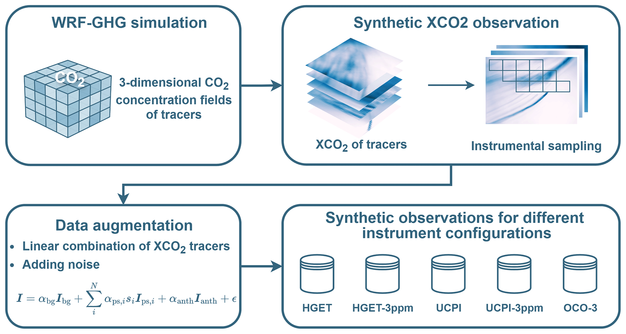
Due to the limited coverage of current OCO-2/3 observations and the inherent retrieval noise from instrumental and prior uncertainties, the current observation data are insufficient for deep learning training, especially for future missions. In this regard, simulation-based approaches are widely adopted in the spaceborne GHG monitoring domain, as demonstrated by studies such as Varon et al. (2018), Jongaramrungruang et al. (2022), Radman et al. (2023), and Dumont Le Brazidec et al. (2024). The Weather Research and Forecasting (WRF) model is commonly used to simulate city-scale atmospheric CO₂ transport (Zheng et al., 2019; Lei et al., 2022; Nerobelov et al., 2023). WRF-GHG (Beck et al., 2011) is a specialized branch of WRF for GHG simulation. Comparisons with observations show that high-resolution WRF-GHG simulations can accurately capture CO₂ plumes from power plants (Brunner et al., 2023). We synthesize pseudo-observation datasets using WRF-GHG to train and evaluate the deep learning method. The overall workflow for dataset construction is illustrated in Fig. 1.

1. WRF-GHG is used to simulate the three-dimensional CO₂ concentration for multiple tracers over Shanghai from January to April 2020, with hourly snapshots (Sect. 2.1.1).

2. The column-averaged dry air mole fraction, denoted as XCO₂, is derived from the three-dimensional CO₂ concentration, and the pseudo-observation images are then synthesized for different instrument configurations (Sect. 2.1.2).

3. A data augmentation method is proposed to improve the generalization of the model trained on the spatial-temporal limited dataset (Sect. 2.1.3).

Figure 1 Workflow for generating the synthetic XCO₂ observation dataset.

2.1.1 CO₂ concentration simulation using WRF-GHG

We implement the WRF-GHG model by modifying the WRF 4.6.0 source code (Skamarock et al., 2019). The physical schemes, based on Beck et al. (2011), include the RRTM scheme (Mlawer et al., 1997) for longwave radiation, the Dudhia scheme (Dudhia, 1989) for shortwave radiation, the Kain-Fritsch cumulus parameterization (Kain, 2004) for the outermost domain, the YSU scheme (Hong et al., 2006) for the planetary boundary layer (PBL) parameterization, the Monin-Obukhov scheme (Monin and Obukhov, 1954) for the surface layer, the WSM5 scheme (Hong et al., 2004) for microphysics, and the NOAH scheme (Chen and Dudhia, 2001) for land surface model (LSM). The simulation domain focuses on Shanghai, China, using a 3-layer one-way nesting setup (Fig. 2). The innermost domain has a resolution of 0.5 km × 0.5 km, to match the ground pixel size of HGET of TanSat-2, while the outermost domain has a resolution of 12.5 km × 12.5 km given grid ratios of 5. The innermost domain spans 110 km × 150 km, encompassing most of the land area of Shanghai. The vertical grid has 50 layers, with the top at 5 kPa. The model runs continuously from 1 January, to 30 April 2020, and produces snapshots at 1 h intervals. In each snapshot, the plumes and background CO₂ concentrations are stored as different tracers.

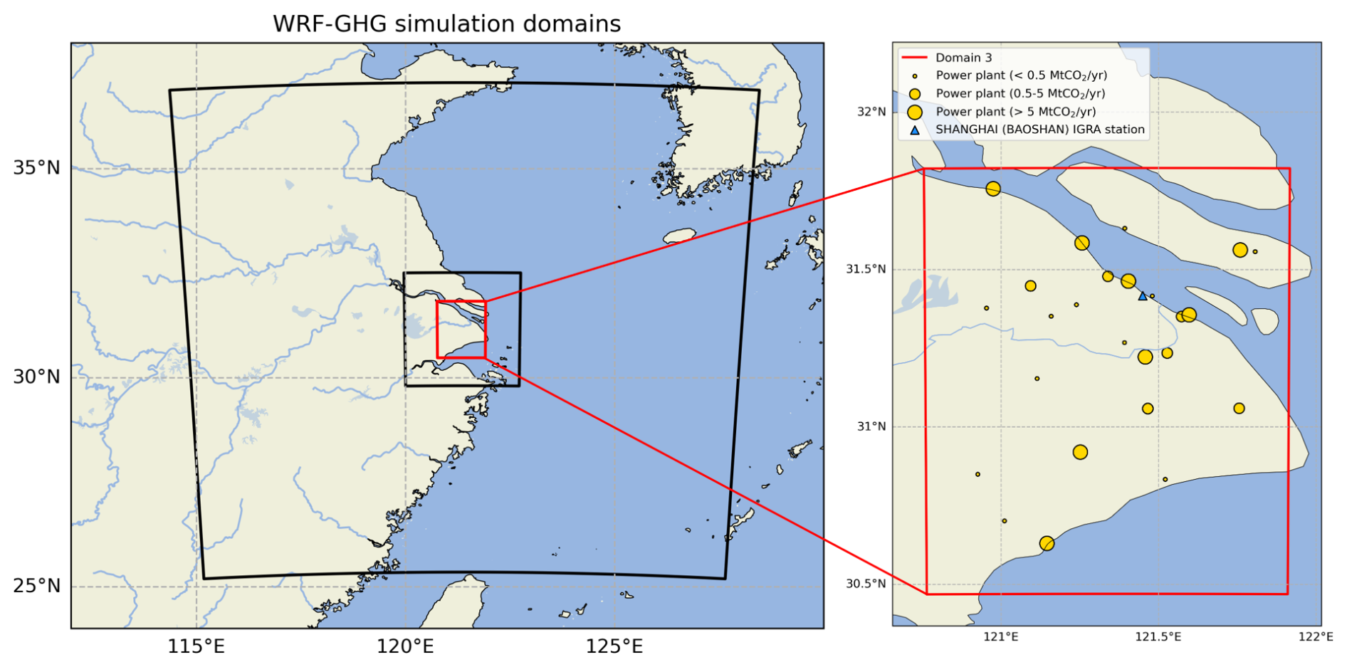
Figure 2 WRF-GHG simulation domain settings. The left panel outlines the three nested domains, while the right panel demonstrates the distribution of major point sources (indicated by circles) and the Baoshan radiosonde station (indicated by a triangle) within the innermost domain.

The primary driving data for the simulation are summarized in Table 1. The Meteorological inputs are derived from the NCEP Final (NCEP-FNL; National Centers for Environmental Prediction et al., 2015) dataset, with a temporal resolution of 6 hours and a spatial resolution of 0.25° × 0.25°. Lateral boundary conditions for background CO₂ are derived from CarbonTracker 2022 (Jacobson et al., 2023). Power plant emissions are treated as point sources, with locations, emission rates and temporal profiles obtained from the CoCO2 dataset (Guevara et al., 2024). Power plants within 0.5 km of each other are merged, and the top 10 facilities (accounting for 79.13 % of total energy-related emissions in Shanghai) are modeled as individual tracers for analysis and data augmentation. Remaining anthropogenic emissions are derived from the EDGAR Community GHG Emissions database v8.0 (Crippa et al., 2024), with temporal profiles from Crippa et al. (2021) to better capture the CO₂ variability. The EDGAR dataset, at 0.1° resolution, is relatively coarse compared to our simulation grid of 0.5 km. Higher-resolution emission data could potentially improve spatial details, as suggested by Kuik et al. (2016), to better capture local concentration patterns. In this regard, similar to Bisht et al. (2023), we utilize local population, road, and land-use data as proxies to redistribute the downscale EDGAR emissions to the model grid. The biomass CO₂ fluxes are pre-calculated using the VPRM model (Mahadevan et al., 2008) and the ocean CO₂ fluxes data are derived from the GONGGA inversion dataset (Jin et al., 2024).

(National Centers for Environmental Prediction et al., 2015)(Jacobson et al., 2023)(Guevara et al., 2024)(Crippa et al., 2024)(Mahadevan et al., 2008)(Jin et al., 2024)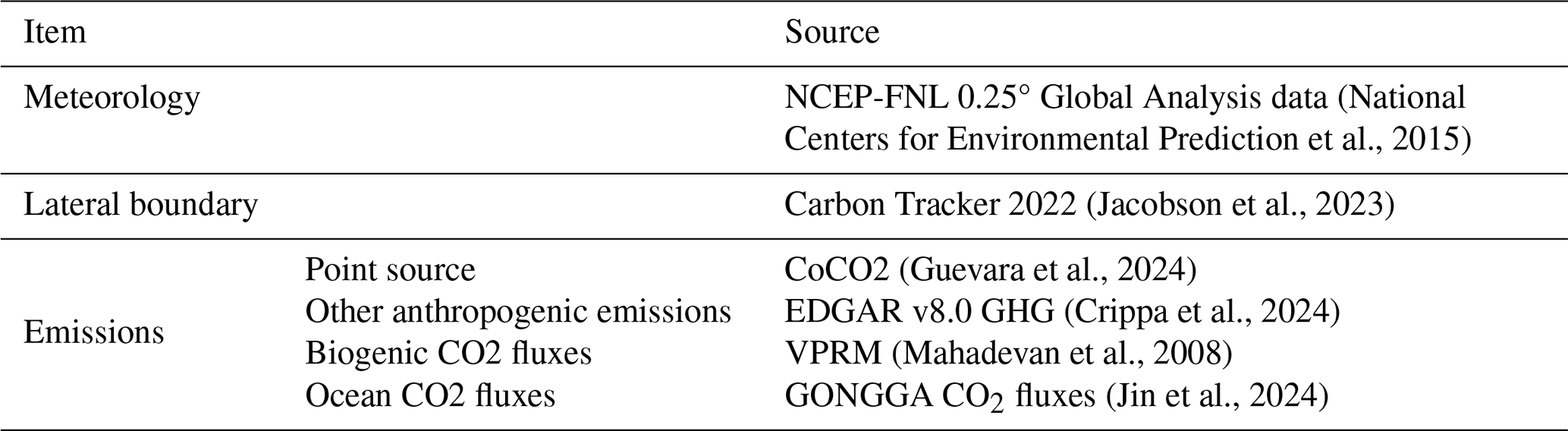

Table 1 Configuration of driving data for WRF-GHG simulations.

2.1.2 Synthetic XCO₂ observation dataset

The column-averaged dry air mole fraction, denoted as XCO₂ with uint parts per million (ppm), is derived from the three-dimensional CO₂ concentration of the tracers, and is given by

$$\begin{array}{}\text{(1)}& X{\mathrm{CO}}_{\mathrm{2}}={\displaystyle \frac{{\mathrm{VCD}}_{{\mathrm{CO}}_{\mathrm{2}}}}{{\mathrm{VCD}}_{\mathrm{dryair}}}}={\displaystyle \frac{{\sum }_i{\mathrm{VCD}}_{\mathrm{dryair},i}\times X{{\mathrm{CO}}_{\mathrm{2}}}_i}{{\mathrm{VCD}}_{\mathrm{dryair},i}}},\end{array}$$

where ${\mathrm{VCD}}_{{\mathrm{CO}}_{\mathrm{2}}}$ denotes the total vertical column density of CO₂, VCD_dryair denotes the total vertical column density of dry air. $X{{\mathrm{CO}}_{\mathrm{2}}}_i$ and VCD_dryair,i denote the CO₂ volume mixing ratio and vertical column density of dry air in ith layer of the model, respectively, and are provided by the model output.

Pseudo-observation XCO₂ images are synthesized using WRF-GHG output in the innermost domain at a 500 m × 500 m horizontal resolution, after applying shift, rotation, and downsampling procedures as described in Pang et al. (2025). The downsampling process simulates the ground pixel size of different instruments and the resulting images are then cropped to approximately 100 km × 100 km. Retrieval noise is then added to the images, with a data augmentation approach for tracers outlined in Sect. 2.1.3. The retrieval noise is determined by instrumental noise and illumination, which is further defined by observation geometry, surface reflectance, aerosol optical depth, etc., such as analysed by Galli et al. (2014) and Jongaramrungruang et al. (2021). A detailed noise formulation is beyond the scope of this work, so it is treated as uncorrelated Gaussian noise.

Here, we consider five different instrument configurations, including low-retrieval-noise (1.5 ppm) and high-retrieval-noise (3 ppm) scenarios for both HGET and UCPI of TanSat-2, as well as the OCO-3 instrument. The instrument configurations, including ground pixel size, image size and noise level, are shown in Table 2. Five datasets are synthesized using different instrument configurations, respectively. Each dataset contains 24 000 XCO₂ concentration maps along with the corresponding source locations and emission strengths. Examples of the synthesize XCO₂ observations for the HGET instrument are shown in Fig. 3, and more examples for other instruments are shown in the Supplement.

Table 2 Instrumental configurations for pseudo-observation.

^* Eldering et al. (2019).

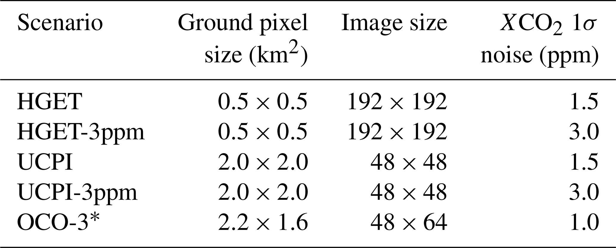
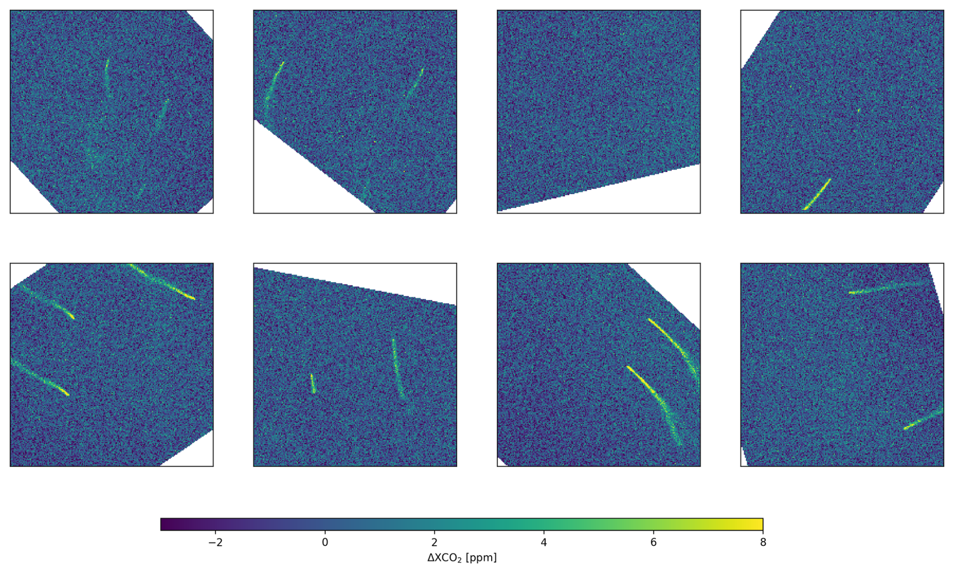
Figure 3 Snapshots of synthesized observation by HGET across multiple footprints. Each map shows the deviation of XCO₂ from the regional average (ΔXCO₂, in ppm). It is worth noting that ΔXCO₂ is only used for visualization purposes, while the inputs to GHGPSE-Net are the original XCO₂ values.

2.1.3 Data augmentation

We propose a data augmentation method to improve the generalization of models trained on spatially and temporally limited datasets by rescaling tracer concentrations, both directly and in proportion to emission rates. CO₂ is chemically inactive in the atmosphere, as a result, its concentration is proportional to the emission rate, based on mass conservation. This relationship allows CO₂ to scale concentrations by emission rates in spaceborne GHG monitoring simulations, such as Jongaramrungruang et al. (2022) and Sánchez-García et al. (2022). Similar to Dumont Le Brazidec et al. (2024), the concentration map can be expressed as a linear combination of various tracers, given by

$$\begin{array}{}\text{(2)}& \mathit{I}={\mathit{\alpha }}_{\mathrm{bg}}{\mathit{I}}_{\mathrm{bg}}+\sum _i^N{\mathit{\alpha }}_{\mathrm{ps},i}{s}_i{\mathit{I}}_{\mathrm{ps},i}+{\mathit{\alpha }}_{\mathrm{anth}}{\mathit{I}}_{\mathrm{anth}}+\mathit{ϵ}.\end{array}$$

Here ${\mathit{I}}_{\mathrm{bg}},{\mathit{I}}_{\mathrm{ps},i}$ and I_anth denote the background CO₂ concentration, CO₂ from ith of total N point sources and CO₂ from other anthropogenic sources, respectively. α_bg, α_ps,i and α_anth denote the corresponding scaling factors. The emission rates are scaled accordingly. s_i denotes a binary switch variable for the ith point source. The scaling factors and switching variables are derived from random distributions. ϵ denotes the observation noise, which is simplified as Gaussian noise.

We introduce three scaling factors, given by

$$\begin{array}{}\text{(3)}& {\mathit{\alpha }}_{\mathrm{bg}}={\displaystyle \frac{c_{\mathrm{bg}}}{\left|{\mathit{I}}_{\mathrm{bg}}\right|}},{\mathit{\alpha }}_{\mathrm{ps},i}={\displaystyle \frac{e_{\mathrm{ps},i}}{e_{\mathrm{ps},i}^{\mathrm{ref}}}},{\mathit{\alpha }}_{\mathrm{anth}}={\displaystyle \frac{e_{\mathrm{anth}}}{e_{\mathrm{anth}}^{\mathrm{ref}}}}.\end{array}$$

Here, $\left|{\mathit{I}}_{\mathrm{bg}}\right|$ denotes the mean concentration of the background CO₂ tracer from the WRF-GHG output; $e_{\mathrm{ps},i}^{\mathrm{ref}}$ and $e_{\mathrm{anth}}^{\mathrm{ref}}$ denote the reference emission rate for the ith point source and the non-point-source anthropogenic sources, respectively. c_bg, e_ps,i and e_anth are random scalars drawn from several distributions. To account for the observed correlation between emissions and background concentrations, as noted by such as Hakkarainen et al. (2016), c_bg and e_anth are sampled from their empirical joint distribution, estimated using EDGAR emission data (Crippa et al., 2024) and CarbonTracker XCO₂ data (Jacobson et al., 2023) in global CO₂ hotspot areas, specifically, 100 km × 100 km areas surrounding power plants emitting over 5 MtCO₂ yr⁻¹. c_bg is then adjusted to track the predicted global mean XCO₂ under SSP1-2.6 (Meinshausen et al., 2020), i.e., the 2 °C scenario of the Paris Agreement, spanning the full lifetime of the TanSat-2 mission. Each e_ps,i is sampled from the major power plants in the CARMA v3.0 inventory (Ummel, 2012). Finally, we introduce binary switch variables, s_i∼Bernoulli(p), where N×p is the expectation of the quantities of power plants within the sampling area. The Supplement provides further details on the relevant distributions.

2.2 Deep neural network for GHG point source extraction (GHGPSE-Net)

A key goal of spaceborne GHG point source monitoring is the efficient and accurate detection, localization, and quantification of emission sources. This is essential for source attribution (Rafiq et al., 2020) and for coordinating with other observational missions (Irakulis-Loitxate et al., 2022; Chiba et al., 2019), particularly when the satellite spatial resolution is sparse. Traditional segmentation-based methods, however, cannot extract both source locations and emission rates automatically from a single concentration map.

Over the past decade, the remote-sensing community has widely adopted the deep learning based object-detection techniques, which focus on object localization and classification rather than pixel-wise segmentation (Zhang et al., 2023). There are two main paradigms, anchor-based neural network and anchor-free neural network. The anchor-based networks, such as Single Shot MultiBox Detector (SSD) (Liu et al., 2016) and Mask Region-based Convolutional Neural Network (Mask R-CNN) (He et al., 2017), predict bounding boxes directly. In contrast, anchor-free networks, such as CornerNet (Law and Deng, 2019) and CenterNet (Duan et al., 2019), extract object centers as key points. CenterNet, in particular, generates a heatmap with peaks corresponding to object centers whose intensities represent attributes such as length, width and orientation (Zhou et al., 2019).

Inspired by CenterNet (Duan et al., 2019), we propose GHGPSE-Net (shown in Fig. 4), a CNN-based model that converts an XCO₂ concentration map into an emission heatmap composed of Gaussian kernels, as to mitigate human interventions. Source locations and emission rates are then derived using Gaussian kernel fitting (GKF).

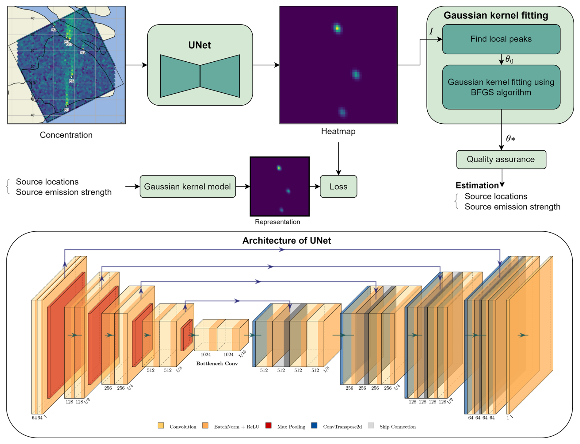
Figure 4 Overview of the proposed GHGPSE-Net architecture. Point sources are represented by a heatmap generated using Gaussian kernels, and a UNet is trained to predict this heatmap from the concentration map. Source locations and emission strengths are then inferred from the predicted heatmap through Gaussian kernel fitting. The lower panel demonstrates the UNet design used in this work. The architecture of UNet is visualized using PlotNeuralNet (Iqbal, 2018).

2.2.1 Deep learning model for heatmap prediction

We represent GHG point‐source emissions as a heatmap generated by the summation of a series of two‐dimensional Gaussian kernels, serving as the neural network's learning target. Each kernel's center and amplitude correspond to the source location and the emission rate. At pixel coordinate $\mathit{x}=[x,y{]}^T$, the heatmap is given by

$$\begin{array}{}\text{(4)}& I\left(\mathit{x}\right)=\sum _{i=\mathrm{1}}^N{a}_{i}G(\mathit{x};{\mathit{\mu }}_i),\end{array}$$

where a_i≥0 denotes the scale of the ith kernel centered at ${\mathit{\mu }}_i=[{\mathit{\mu }}_{x,i},{\mathit{\mu }}_{y,i}{]}^T$. The Gaussian function G is given by

$$\begin{array}{}\text{(5)}& G(\mathit{x};{\mathit{\mu }}_i)=\exp \left(-{\displaystyle \frac{\mathrm{1}}{\mathrm{2}}}{\displaystyle \frac{(\mathit{x}-{\mathit{\mu }}_i{)}^T(\mathit{x}-{\mathit{\mu }}_i)}{{\mathit{\sigma }}^{\mathrm{2}}}}\right),\end{array}$$

where σ defines the spatial extent (hereafter intuitively referred to as the kernel size).

We train a CNN deep learning model using supervised learning to infer emission heatmaps from XCO₂ concentration maps. Deep neural networks are a class of universal machine learning algorithms, which have been mathematically proved to approximate any continuous real function within a hypercube (Cybenko, 1989). A CNN primarily consists of convolutional layers, activation functions, pooling layers and linear layers, allowing it to extract compact feature representations from complex, sparse inputs. Popular image-to-image CNN architectures, such as UNet (Ronneberger et al., 2015) and HourglassNet (Newell et al., 2016), preserve spatial resolution with output feature maps similar in size to the input images, making them suitable for emission heatmap inference.

We select UNet as the CNN model. UNet features a symmetric encoder-decoder structure with skip connections (shown in Fig. 4), which preserves spatial information and enables multi-scale feature fusion. UNet has been proven effective for spaceborne GHG plume segmentation tasks (Dumont Le Brazidec et al., 2023; Vaughan et al., 2024). To adapt the original UNet from classification to heatmap prediction, the final softmax layer is replaced with a convolution layer. The UNet model is implemented using the PyTorch framework (Paszke et al., 2019).

2.2.2 Gaussian kernel fitting

To extract point objects from predicted heatmaps, traditional non-maximal suppression (NMS) uses the local peak pixels to represent the object (Law and Deng, 2019), which limits the accuracy in subpixel localization. In this regard, we infer source locations and emission rates by fitting predicted heatmaps using Gaussian kernel functions. Let the parameter vector be denoted as $\mathit{\theta }=[{\mathit{a}}^T,{\mathit{\mu }}_x^T,{\mathit{\mu }}_y^T{]}^T$, where $\mathit{a}=[a_{\mathrm{1}},a_{\mathrm{2}},\mathrm{\dots },a_N{]}^T$; ${\mathit{\mu }}_x=[{\mathit{\mu }}_{x,\mathrm{1}},{\mathit{\mu }}_{x,\mathrm{2}},\mathrm{\dots },{\mathit{\mu }}_{x,N}{]}^T$; ${\mathit{\mu }}_y=[{\mathit{\mu }}_{y,\mathrm{1}},{\mathit{\mu }}_{y,\mathrm{2}},\mathrm{\dots },{\mathit{\mu }}_{y,N}{]}^T$. Let P denote the number of pixels and x_p denote the location of the pth pixel. We can then estimate the parameters θ by fitting the modeled image $\widehat{\mathit{I}}$ to the heatmap I using constrained least squares, given by

$$\begin{array}{}\text{(6)}& {\mathit{\theta }}^{*}={\mathrm{argmin}}_{\mathit{\theta }}\mathcal{L}(\mathit{\theta };\mathit{I},\widehat{\mathit{I}}),\end{array}$$

where the cost function is given by

$$\begin{array}{}\text{(7)}& \begin{array}{rl}\mathcal{L}(\mathit{\theta };\mathit{I},\widehat{\mathit{I}})& =\sum _{p=\mathrm{1}}^P{\left(I\left({\mathit{x}}_p\right)-\widehat{I}({\mathit{x}}_p;\mathit{\theta })\right)}^{\mathrm{2}}\\ & \mathrm{s}.\mathrm{t}.a_i\ge \mathrm{0},\forall a_i\in \mathit{a}.\end{array}\end{array}$$

We transform the constrained problem into an unconstrained least squares formulation through a penalty term and solve it using the BFGS method (Nocedal and Wright, 2006). The BFGS method is a quasi-Newton method that has the advantage of not requiring expensive second-order derivative computations because it approximates the Hessian matrix, leading to faster convergence. The estimated emission rates are adjusted by the ratio of local pressure to the average reference pressure in the dataset. Implementation details are provided in the Supplement.

2.2.3 Experiment setup

The models are trained from scratch using supervised learning on 24 000 simulated observation snapshots for each instrument scenario (Sect. 2.1.2), respectively. Each dataset is divided randomly into training, validation, and testing sets in a $\mathrm{3}:\mathrm{1}:\mathrm{1}$ ratio. The model is trained using the training sets, where the model weights are updated by minimizing the mean squared error (MSE) between the CNN-predicted and true heatmaps (modeled by Eq. 4). The Adam optimizer is used for training with an initial learning rate of 0.001 and a batch size of 16. The models generally converge within 30 epochs. The model with the lowest validation loss at each epoch is selected for final evaluation on the test set. In the evaluation stage, the model not only predicts the heatmap but also generates source locations and emission strengths using GKF. Evaluation details are described in Sect. 2.3.

2.3 Evaluation

2.3.1 WRF-GHG simulation evaluation

We evaluate the accuracy of our WRF-GHG simulation by comparing the meteorological variables and XCO₂ against independent observations. The modeled meteorological outputs, including temperature and wind, are compared against radiosonde profiles from the Integrated Global Radiosonde Archive (IGRA) Version 2 (Durre et al., 2016) at Baoshan station, which locates within the 0.5 km × 0.5 km innermost domain of the WRF-GHG simulation (Fig. 2). The simulated XCO₂ is evaluated against OCO-3 retrievals (v10.4r) in snapshot area maps (OCO-2/OCO-3 Science Team et al., 2022). To avoid discrepancies in XCO₂ caused by differences in vertical weighting methods, XCO₂ are calculated using the modeled profiles, a priori profiles, and column averaging kernels from the OCO-3 standard product. This approach is used for the evaluation, following the method described by Connor et al. (2008); Zheng et al. (2019), rather than the direct synthesis approach described in Sect. 2.1.2. The accuracy is assessed using root mean square error (RMSE) to measure the overall error; and mean absolute error (MAE), which is less sensitive to large anomalies compared to RMSE.

2.3.2 Source extraction evaluation

We evaluate the performance of the proposed GHGPSE-Net in three aspects, detection, localization and quantification. Firstly, the predicted and ground-truth sources are paired by solving a linear sum assignment problem with Euclidean distance. Pairs within 4 km are counted as true positives (TP); the unmatched predictions are counted as false positives (FP); and the unmatched ground-truth sources are counted as false negatives (FN). The detection performance is then evaluated by precision, recall and F₁-score, given by

$$\begin{array}{}\text{(8)}& \begin{array}{l}\mathrm{Precision}=\frac{\mathrm{TP}}{\mathrm{TP}+\mathrm{FP}},\\ \mathrm{Recall}=\frac{\mathrm{TP}}{\mathrm{TP}+\mathrm{FN}},\\ F_{\mathrm{1}}=\frac{\mathrm{2}\mathrm{TP}}{\mathrm{2}\mathrm{TP}+\mathrm{FP}+\mathrm{FN}}.\end{array}\end{array}$$

Secondly, for all true positives, we evaluate the Euclidean‐distance errors as the localization accuracy with their mean and median. Finally, we compare the predicted emission rates against the ground truth using the coefficient of determination (R²) to evaluate the overall fitness; Pearson's correlation coefficient (R) to evaluate linear correlation between predictions and actual values, regardless of scale; RMSE, MAE and mean absolute percent error (MAPE) to quantify the errors.

2.3.3 Zero-shot generalization to SMARTCARB simulations and OCO-3 observations

We evaluate the zero-shot generalization of the proposed GHGPSE-Net on two independent datasets. The models are trained using the synthetic datasets and evaluated using the following external datasets.

1. OCO-3 SAM observations over U.S. power plants.

   OCO-3 observations in SAM mode provide denser sampling of anthropogenic GHG emission hotspots than its predecessor (Kiel et al., 2021), making it suited for quantifying CO₂ emissions from large point sources globally (Yang et al., 2024; Lin et al., 2023). Due to the relatively limited spatial coverage of OCO-3, most of the observations are faced with issues such as discontinuities by cloud contamination, weak plume signals, and background anthropogenic emissions, we only select8 observations covering 4 major power plants (>1 ktCO₂ h⁻¹) with relatively clear and spatially isolated plumes from the OCO-3 Level 2 v10.4r dataset (OCO-2/OCO-3 Science Team et al., 2022) for reliable evaluation. The OCO-3 observations are interpolated onto the regular Cartesian grid (described in Table 2) as the model inputs. Discontinuous missing data points in OCO-3 sampling are filled using the mean value. Inventory emission rates from the Clean Air Markets Program Data (CAMPD) (EPA, 2021) are used as the ground truth.

2. SMARTCARB simulations.

   To supplement the relatively sparse OCO-3 observations, we also evaluate GHGPSE-Net on the SMARTCARB simulation dataset (Kuhlmann et al., 2019b), which was generated using the Consortium for Small-scale Modelling (COSMO)-GHG model rather than WRF-GHG. The SMARTCARB dataset provides one year of hourly XCO₂ simulations at 1.1 km spatial resolution, covering Berlin and surrounding major power plants, where the emission rates are derived from the TNO-MACC II inventory (Kuenen et al., 2014). We evaluate the source extraction performance of GHGPSE-Net using 998 snapshots covering major power plants, including Boxberg, Jänschwalde, Lippendorf, and Schwarze Pumpe in Germany, and Turów in Poland.

3 Results

3.1 WRF-GHG simulation accuracy

First, we compare the WRF-GHG simulated temperature, wind speed, wind direction against radiosonde profiles from IGRA v2.0. As the dispersion tracers are largely confined to the planetary boundary layer (Al-Hemoud et al., 2019), we focus the comparison of meteorological variables to near-surface conditions, approximated by the 1000 hPa pressure level. As shown in Fig. 5, the WRF-GHG simulation demonstrates reasonable agreement with observations for most meteorological variables. Temperature errors are mostly within ±3 K, with an RMSE of 4.4 K and MAE of 3.2 K, indicating that the temperature is well reproduced by WRF-GHG. Wind speed errors show an RMSE of 2.9 m s⁻¹ and MAE of 2.3 m s⁻¹, suggesting that the WRF-GHG effectively captures wind magnitude. Wind direction errors, however, exhibit larger discrepancies, with an RMSE of 82.49° and an MAE of 62.98°, reflecting notable discrepancies with observations. For dew point temperature, the RMSE and MAE are 7.3 and 5.6 K, respectively, demonstrating moderate accuracy in representing atmospheric moisture conditions.

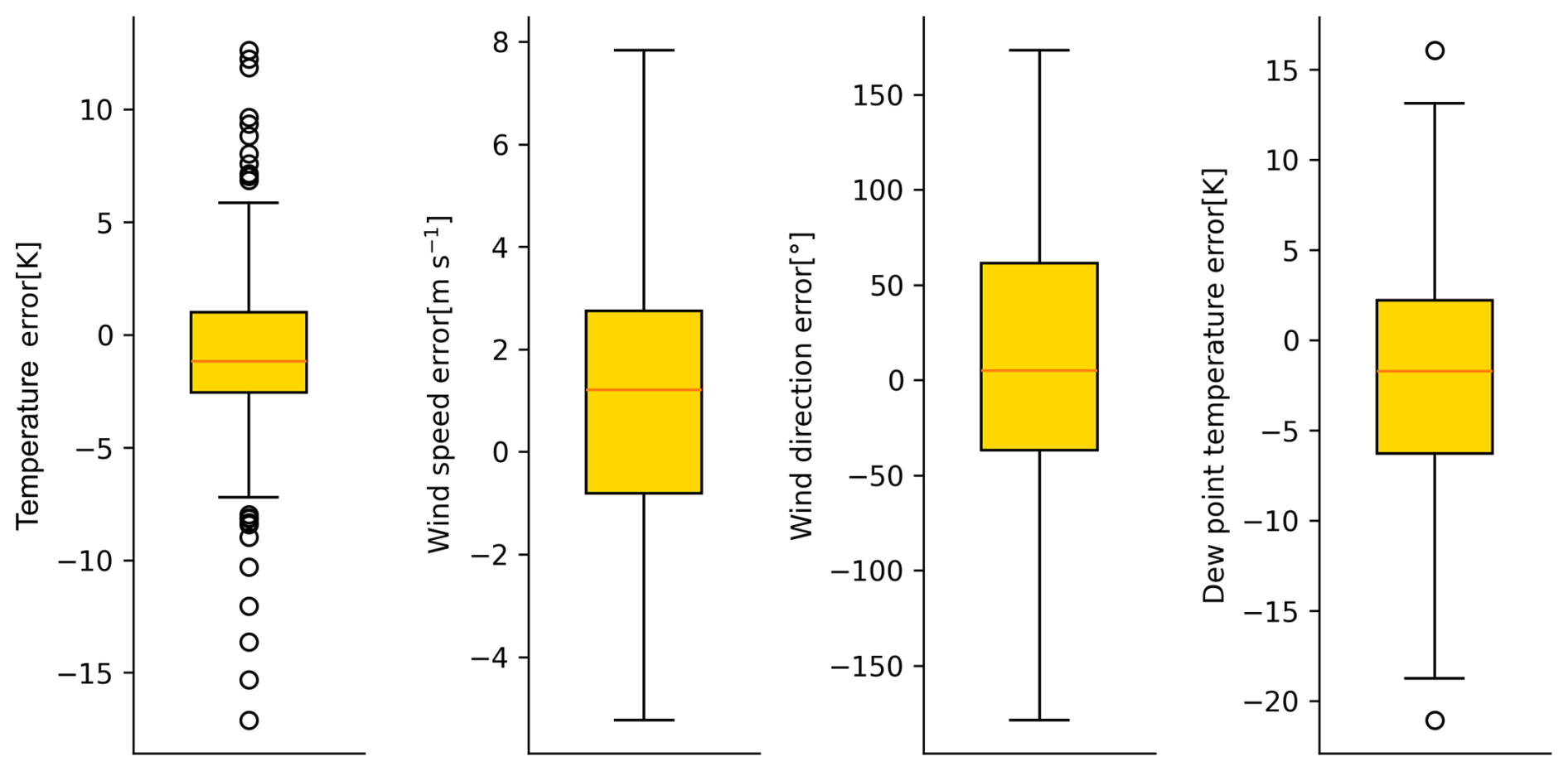
Figure 5 Residual distribution of meteorological variables generated by WRF-GHG compared to IGRA v2.0 measurements at Baoshan station. In each boxplot, the orange dash denotes the median, the box denotes the range between the lower and upper quartiles, the whiskers extend from the box by 1.5 times the interquartile range (IQR), and the circles denote the outliers.

Second, we assess WRF-GHG's capability to model XCO₂ against OCO-3 retrievals. As shown in Fig. 6, there are three clear-sky OCO-3 passes above Shanghai (20 February, 24 February, and 23 April 2020, UTC) within the simulation running time range, with a total of 1326 retrieval samplings. In general, the WRF-GHG model well reproduces OCO-3 observed XCO₂ with an RMSE of 1.58 ppm, MAE of 1.16 ppm, and Pearson's R of 0.75. A small subset of points, most of which are located downwind of urban or heavy‐industry sources during the 20 February and 23 April passes, exhibit absolute errors >3 ppm (Supplement), while the majority of the remaining samples fall within ±1 ppm.

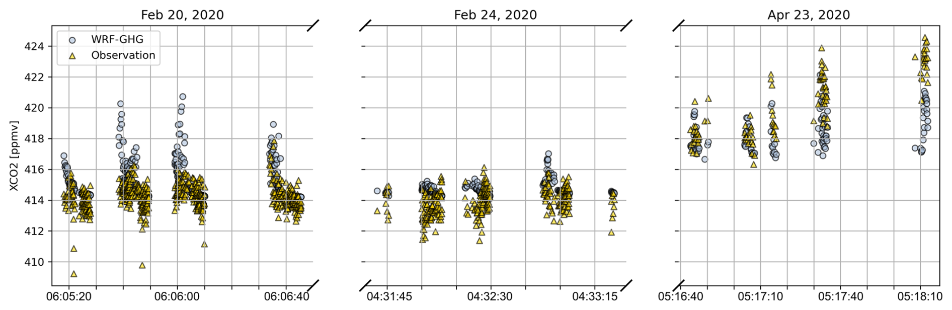
Figure 6 Comparison between XCO₂ simulated by WRF-GHG and that retrieved from OCO-3 observations. The observation timestamps are provided in UTC. The large deviations in 20 February and 23 April 2020 are mostly observed downwind of urban or heavy‐industry sources (Supplement).

3.2 Overall evaluations of the proposed method

We evaluate the influence of Gaussian kernel fitting (GKF) and the choice of kernel size (σ) on the performance of the proposed GHGPSE-Net. Experiments are conducted using the HGET instrument dataset of Table 2. We compare the extraction performance of GHGPSE-Net with and without GKF, where the sources are derived directly from the local peak pixels of the heatmap, i.e., the pixel locations and their corresponding values represent the source locations and emission rates, respectively. Additionally, we also compare the performance over kernel sizes, both with and without GKF.

As shown in Fig. 7, when the kernel size matches the instrument's spatial resolution (500 m) and GKF is applied, the model achieves its best overall performance. Qualification metrics reach their peaks with a Pearson's R of 0.99, R² of 0.98, RMSE of 89.9 tCO₂ h⁻¹, MAE of 57.7 tCO₂ h⁻¹, and MAPE of 0.05. Detection metrics reach peaks with precision of 0.98, recall of 0.95, and F₁-score of 0.96, indicating that most point sources are correctly detected and accurately quantified. Deviating from 500 m, both quantification and detection performance deteriorate, with quantification metrics beginning to regrow at σ above 1500 m. Applying GKF brings a slight improvement in quantification at the small σ cases, where the R² improves from 0.36 to 0.54, and RMSE decreases from 556.6 to 473.4 tCO₂ h⁻¹. Detection metrics are not sensitive to the GKF procedure.

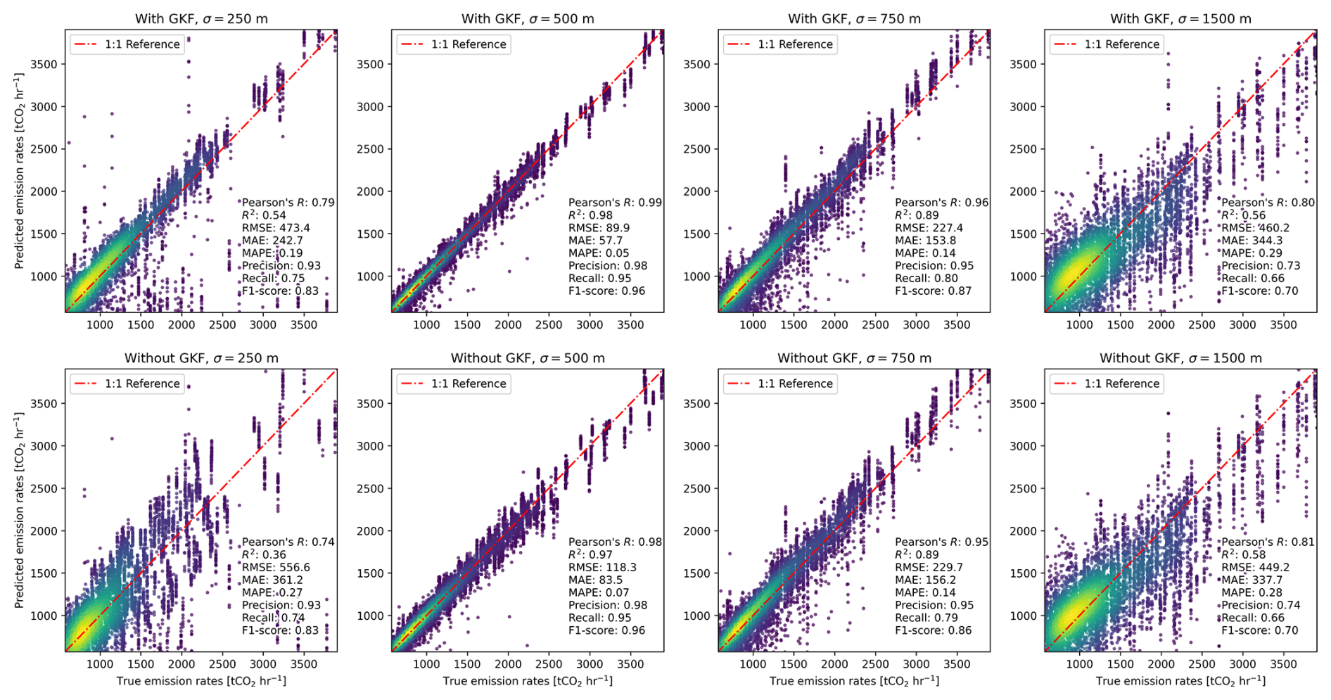
Figure 7 Scatter plots comparing GHGPSE-Net under various settings. Each plot shows results from experiments with (top row) and without (bottom row) the Gaussian kernel fitting (GKF) process, across different kernel sizes (σ=250, 500, 750, and 1500 m from left to right). Predicted emissions are plotted against true emissions. Each plot includes quantification performance metrics, including Pearson's R, R², RMSE, MAE, and MAPE, as well as detection indicators, including precision, recall, and F₁-score.

We further investigate the influence on localization of GKF and kernel size. As shown in Fig. 8, small kernel size improves locating accuracy. Moreover, GKF largely reduces the locating errors, where the mean error decreases from 199.5 to 61.4 m, and the median error from 200.1 to 49.7 m. These errors are well below the 500 m spatial resolution, indicating the model is capable of subpixel-level source localization.

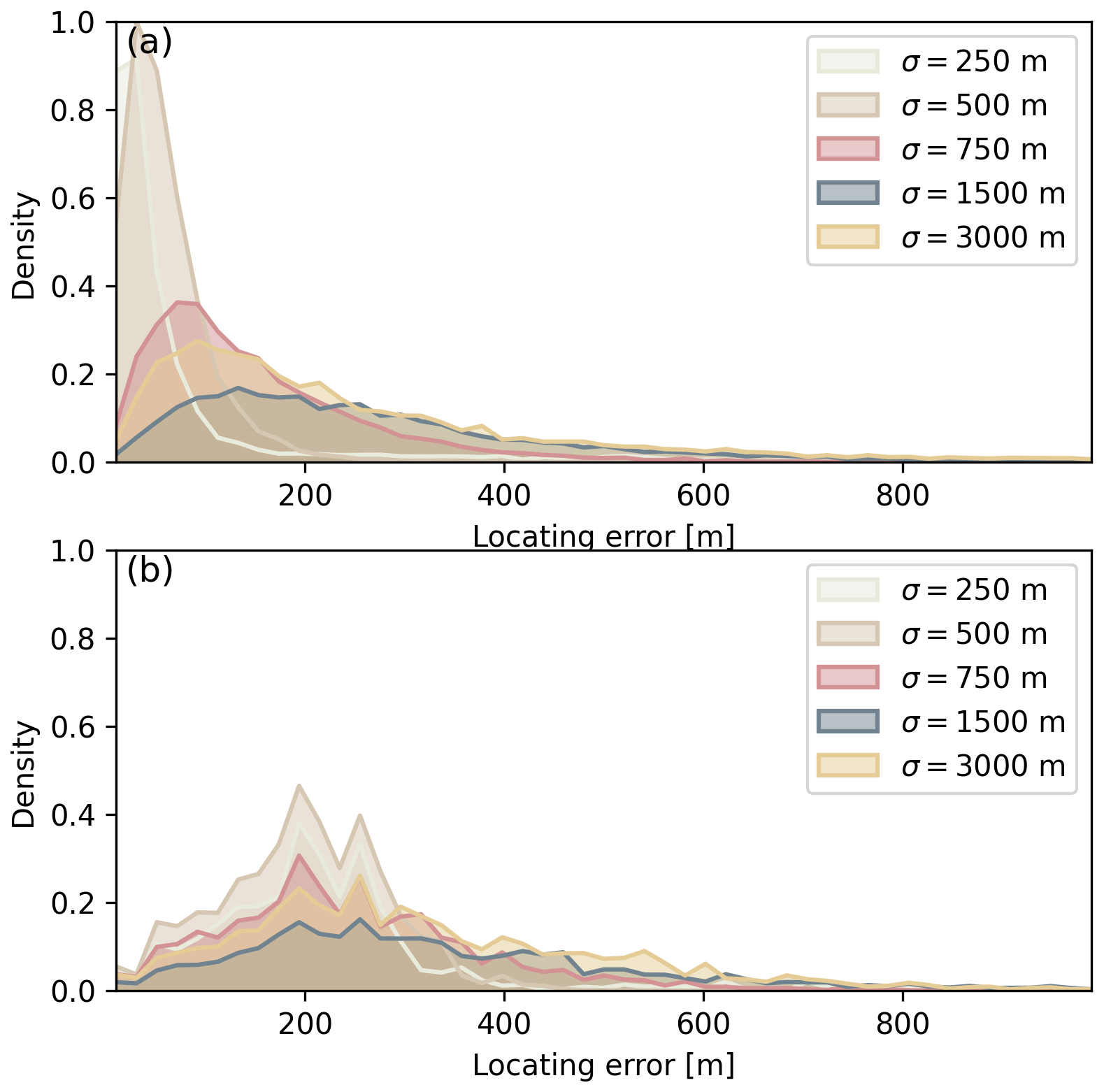
Figure 8 Distribution of locating errors for GHGPSE-Net under different settings. Each curve represents the normalized probability density function (PDF) for a specific experiment, scaled to the overall maximum value. Panel (a) shows results with the Gaussian kernel fitting (GKF) process, while panel (b) shows results without GKF.

3.3 Comparative assessment of different instrument configurations

We evaluate the performance of GHGPSE-Net across various instrument configurations, including low-noise (1.5 ppm) and high-noise (3 ppm) retrieval scenarios for HGET onboard TanSat-2, as well as the UCPI instrument, dedicated to GHG point source monitoring. We also test the model on simulated observations with spatial resolution and retrieval noise matching those of OCO-3, which is widely used for global point source monitoring. The following experiments are conducted with the GKF process. The kernel size of GKF is set to match each instrument's spatial resolution, i.e., 500 m for HGET, 2 km for UCPI, and 2.2 km for OCO-3, in the following text.

As shown in Table 3, GHGPSE-Net achieves the best performance in detection, localization, and quantification with the low-noise HGET configuration. In comparison, the UCPI scenario shows degraded performance, with localization errors increasing nearly four times and quantification errors increasing to 2.6–2.8 times. The performances also deteriorate under higher retrieval noise for both instruments. Notably, the HGET-3ppm case performs worse than UCPI-3ppm in recall (0.54 v.s. 0.63) and quantification (0.50 v.s. 0.72 in R² and 0.28 v.s. 0.21 in MAPE), indicating that while HGET benefits from its fine spatial resolution, it is more sensitive to uncorrelated Gaussian noise. Although OCO-3 has retrieval noise slightly lower to UCPI and features a smaller ground pixel area (2.2×1.6 km² v.s. 2×2 km²), UCPI achieves better performance in both localization and quantification. This suggests that the smaller pixel area of OCO-3 does not compensate for the limitations brought by its narrow shape pixel with a longer along-track dimension.

Table 3 Performance comparison of GHGPSE-Nets on different instrument configurations.

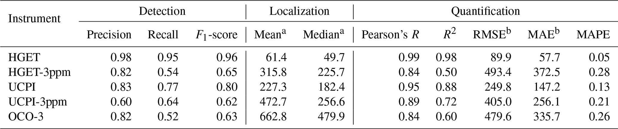
^a with unit [m]. ^b with unit [tCO₂ h⁻¹].

3.4 Generalization evaluation using SMARTCARB dataset and OCO-3 observation

We first evaluated the impact of data augmentation on the model's generalization performance. Compared to the baseline GHGPSE-Net with augmentation, the model trained without augmentation demonstrates substantial performance decline, where the recall decreases from 0.95 to 0.09, the mean location error increases from 61.4 to 310.2 m, and quantification RMSE increases from 89.9 to 1072.7 tCO₂ h⁻¹ (Supplement).

To further assess the generalization capability of GHGPSE-Net trained on spatially and temporally limited simulations, we evaluate its performance on the SMARTCARB dataset of Berlin, simulated by COSMO-GHG, as well as on OCO-3 observations of power plants in the U.S. For the SMARTCARB case, the model is trained on synthesized observations of the UCPI scenario, but with a lower noise level (standard deviation of 0.7 ppm) to match the SMARTCARB dataset. For the OCO-3 cases, the model is trained using datasets of the OCO-3 scenario.

As shown in Fig. 9, the GHGPSE-Net exhibits considerable generalization on the SMARTCARB dataset. In terms of detection performance, the model achieves a precision of 0.86, which is comparable to its performance on the UCPI scenario. However, the recall and F₁-score are only 0.48 and 0.62, respectively, indicating notable mis-detections. For localization accuracy, the mean and median errors are 1.80 km and 1.49 km, respectively. These values surpass those obtained when testing on the WRF-GHG dataset, yet they remain smaller than the 2 km ground pixel size of the input data, which is enough for providing meaningful spatial locations for joint observation missions. The quantification performance is less robust, with a Pearson's R of 0.26, RMSE of 2.4 ktCO₂ h⁻¹, and MAPE of 0.77. Among the five power plant cases, the model achieves best performance at the Jänschwalde case, with mean reported and predicted emission rates of 4.4 and 4.5 ktCO₂ h⁻¹, respectively. However, the model tends to overestimate emissions at the other four plants, which have comparatively lower emission rates than Jänschwalde, with an MAE of 1.2 to 1.6 ktCO₂ h⁻¹. Further analysis on noise-free SMARTCARB data using GHGPSE-Net trained without noise indicates that the different noise pattern is not the major factor contributing to the undesirable quantification performance, as the quantification performance remains largely unchanged, with a Pearson's R of 0.28, RMSE of 2.5 ktCO₂ h⁻¹, and MAPE of 0.81.

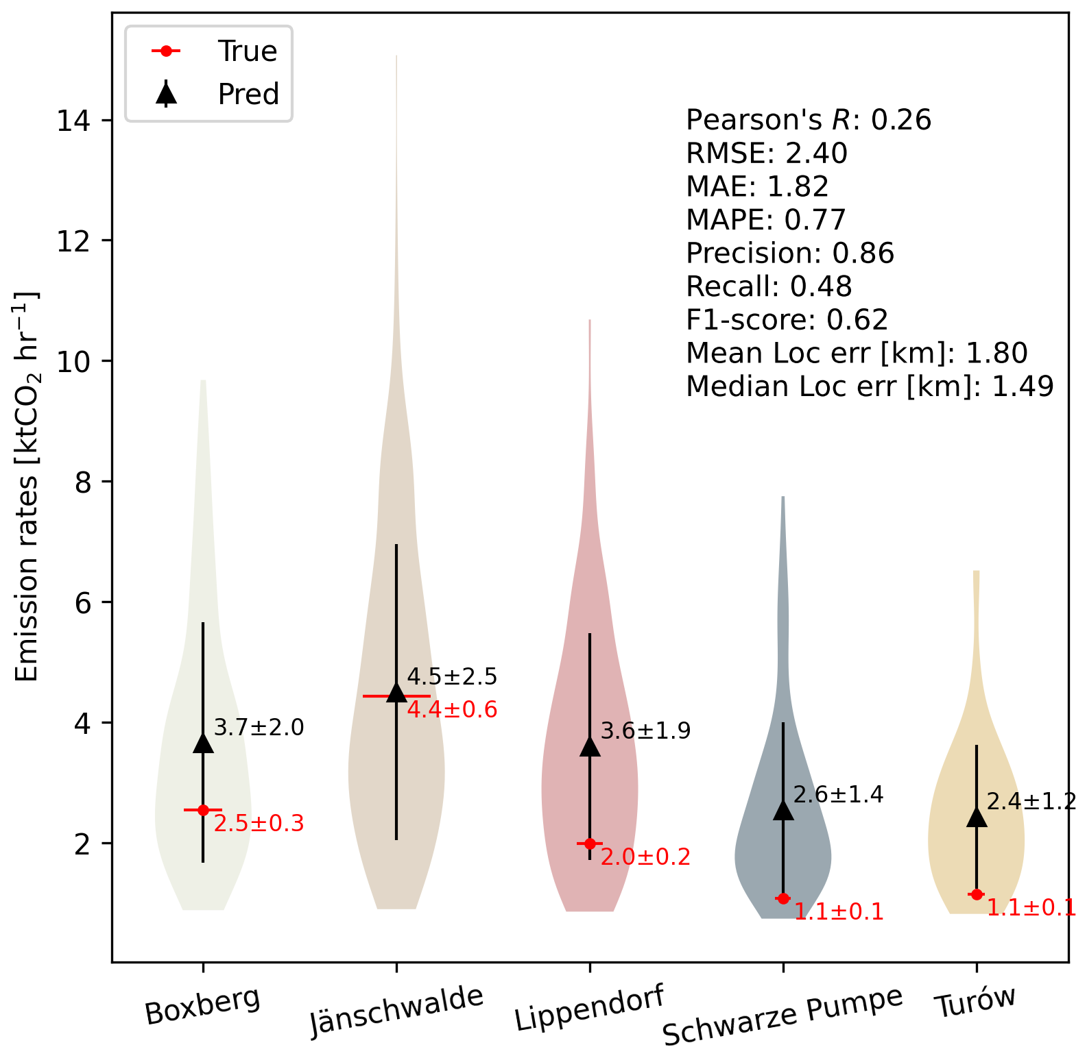
Figure 9 Violin plot illustrating GHGPSE-Net's emission quantification performance across five major power plants from the SMARTCARB dataset. Each violin represents the distribution of predicted emissions. The lines extended to show ±1σ uncertainty with markers at their mean value. The red lines indicate the Ground-truth values from the TNO-MACC II inventory, while the black lines represent GHGPSE-Net's predictions The overall performances of quantification detection and localization are summarized within the panel.

Among the OCO-3 observations, GHGPSE-Net achieves a detection precision of 0.89 with a mean localization error of 3.02 km. We compare the estimated emissions against those reported by the EPA CAMPD inventory. As shown in Table 4, the model identifies several major power plants, including Colstrip, Four Corners Steam Electric Station, Jeffrey Energy Center, and Oak Grove. overall, the quantified emissions agree well with the inventory, with a Pearson's R of 0.59, MAPE of 0.29, RMSE of 0.47 ktCO₂ h⁻¹, and MAE of 0.41 ktCO₂ h⁻¹. In these cases, Colstrip and Jeffrey Energy Center are two relatively isolated power plants with high emission rates, where the model correctly captures and attributes their emissions. The Four Corners Steam Electric Station lies near the San Juan and Bluffview power plants (Fig. 10b), while Oak Grove is located near the Twin Oaks power plant (Fig. 10c–d). In these cases, the emission rates of these smaller nearby power plants are generally under 0.57 ktCO₂ h⁻¹ (i.e., approximately 5 MtCO₂ yr⁻¹) according to the CAMPD inventory, resulting in weak signals that are nearly invisible in the OCO-3 observations.

Table 4 The estimated emission of identified power plants over the U.S.

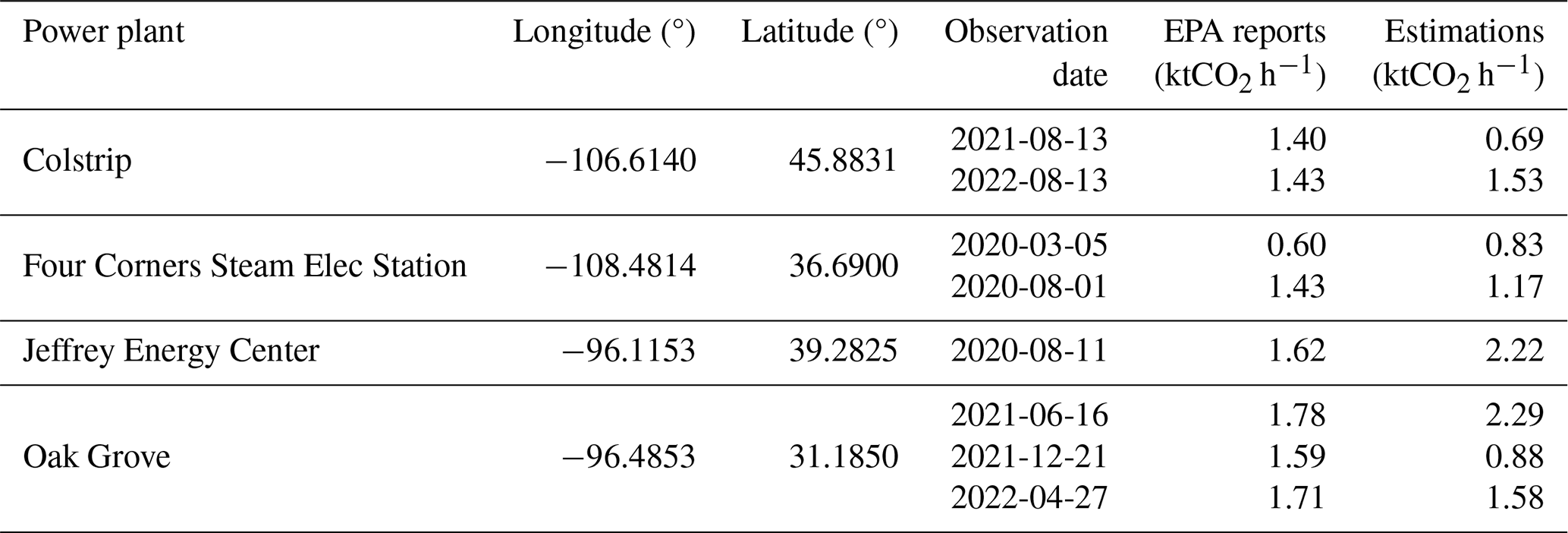
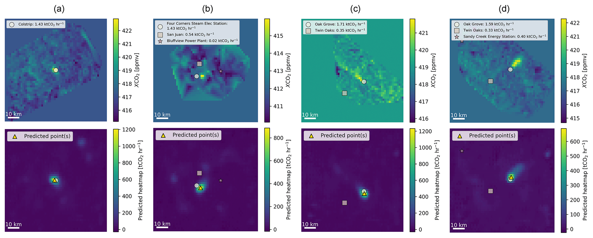
Figure 10 Examples of input OCO-3 observations (top row) and the corresponding GHGPSE-Net predicted heatmaps (bottom row) for power plants in the U.S. The power plants in the EPA CAMPD inventory are marked and labeled with their reported emission rates. The predicted source locations are marked with gold triangles in the heatmaps.

4 Discussions and Conclusion

In this study, we proposed GHGPSE-Net, a deep learning model designed to simultaneously identify the locations and quantify emission rates of GHG point sources. To train and evaluate the model, we modeled the atmospheric CO₂ transport using WRF-GHG and synthesized pseudo-observations with different instrumental configurations. The simulations were evaluated using IGRA and OCO-3 measurements, which demonstrate considerable agreement with observations. We comprehensively evaluated GHGPSE-Net's performance on GHG point source extraction from detection, localization, and quantification. For the proposed method, the impact of Gaussian kernel fitting and the choice of kernel size selection was first assessed. We then analyzed model performance under various idealized instrument configurations. Finally, we assess the model's generalization capabilities using simulations from SMARTCARB and spaceborne observations from OCO-3.

In general, the WRF-GHG model effectively simulated the atmospheric transport of CO₂ over Shanghai, providing a reliable synthetic dataset for training deep learning models to extract emission sources. Overall, the comparison of meteorological variables against radiosonde data suggests that the WRF-GHG model provides a robust and reliable simulation of atmospheric transport conditions, with RMSE of 4.4 K for temperature, 2.9 m s⁻¹ for wind speed, 82.5° for wind direction and 7.3 K for dew point temperature. Here, we mainly focus on the evaluation of the lower troposphere. The influence of upper-tropospheric atmospheric dynamics on anthropogenic CO₂ transport is limited, as most emissions remain within the PBL (Al-Hemoud et al., 2019), where the meteorological conditions are well reproduced by WRF-GHG. The near-surface wind direction may be affected by complex terrain effects and exhibits high uncertainty, the model still captures the general direction of the CO₂ plume at larger spatial scales. The results of WRF-GHG model agree well with OCO-3, particularly for the background field. The discrepancies are mainly observed downwind of major emission sources, indicating possible inaccuracies in the emission inventory. Comprehensive evaluations of the simulation accuracy, particularly its diurnal behavior, will require continuous CO₂ observations, which are currently unavailable in this study.

Based on the synthetic dataset, we evaluated the performance of the proposed deep learning method for greenhouse gas point source extraction (GHGPSE-Net), as well as quantified the impact of model design choices. GHGPSE-Net demonstrated strong performance in source detection (F₁-score of 0.96), localization (mean error of 12.3 % of pixel size), and quantification (Pearson's R of 0.99) in the baseline experiment. The Gaussian kernel size in the heatmap label generation and fitting has a significant impact on the model's performance. A kernel that is too wide tends to blur local features, reducing detection accuracy, while a kernel size that is too narrow tends to bring in overly localized gradients, hindering parameter updates in training. Our experiments indicate that the optimal performance is achieved when the kernel size closely matches the pixel size. The Gaussian kernel fitting (GKF) module, implemented using least-squares optimization and concatenated after the UNet, also plays an important role in GHGPSE-Net. While its impact on detection is limited, it improves quantification moderately (24.0 % reduction in RMSE compared to without GKF for the σ=500 m baseline case) and improves the localization performance substantially (69.2 % reduction in RMSE for the same case). By incorporating global context from the predicted heatmap, the GKF module increases robustness to anomalies and spurious peaks, particularly when using a smaller kernel size.

We evaluated GHGPSE-Net over various instrument configurations with different pixel sizes and retrieval errors. In general, finer pixel resolution yields better performance for point source monitoring, which contributes to capture plume shapes and provides more spatial context for inference. However, finer pixel resolution is also more subjected to increasing retrieval noise. It is also worth noting that, in practice, the observation noise may deviate from Gaussian assumptions (Jongaramrungruang et al., 2022; Radman et al., 2023), as it is mainly driven by illumination conditions including solar zenith and surface albedo. This requires more sophisticated noise modeling, such as the parameterized approach by Kuhlmann et al. (2019b).

We proposed a data augmentation strategy by scaling XCO₂ from different tracers to better accommodate real-world distributions beyond the original simulation domain and time range. The scaling factors reflect more realistic patterns, including future trend, power plant density, correlation between background XCO₂ and anthropogenic emissions, etc, extending from previous strategies such as Dumont Le Brazidec et al. (2024). Models trained without augmentation demonstrate poor source extraction ability due to a significant mismatch between training and test data. In contrast, GHGPSE-Net trained with augmentation demonstrates considerable generalization to both the SMARTCARB simulation and OCO-3 observations. On the SMARTCARB case, GHGPSE-Net achieves high precision (0.86) but moderate recall (0.48), suggesting it can reliably identify strong sources but may miss weaker sources, which is further confirmed by the quantification performance.

These results also reveal notable discrepancies between simulation datasets. One possible explanation is the more realistic vertical emission profiles used in SMARTCARB (Kuhlmann et al., 2019b; Brunner et al., 2019), which are simplified as surface emissions in this work due to the lack of these profiles. This simplification may underestimate the role of emissions entering the free troposphere, which can form new plume shapes with different orientations from those in the PBL (Brunner et al., 2023), potentially leading to false detections (Supplement). Other factors, such as differences in meteorological conditions, terrain effects, and the use of different transport models (COSMO-GHG v.s. WRF-GHG), may also contribute to the discrepancies. On the OCO-3 case, the quantification results generally agree with the inventory (Pearson's R of 0.59, MAPE of 0.29), indicating the model demonstrates considerable generalization to real satellite observations. However, due to the discontinuous and limited coverage of OCO-3, very few samples are identified with point sources. The complex and heterogeneous noise characteristics, discontinuous sampling, diverse plume morphologies, and varying meteorological conditions in real observations also pose challenges to model generalization. The decreased performance on the two independent datasets also suggests that evaluations conducted exclusively on a single synthetic dataset may systematically overestimate model performance, due to the inherent statistical homogeneity within such datasets. Further evaluation using continuous and large-scale XCO₂ measurements from upcoming missions such as TanSat-2, CO2M, and GOSAT-GW is needed to fully assess the model's performance in real applications. Additionally, transfer learning techniques could be explored to further improve model generalization to real-world data.

In this study, we propose GHGPSE-Net, a deep learning model for simultaneous detection, localization, and quantification of GHG point sources. The model is trained and evaluated using synthetic datasets generated from WRF-GHG simulations. Synthetic datasets generated by WRF-GHG are constructed for training and evaluation, accompanied by a data augmentation strategy to enhance model generalization. Results show the model achieves accurate detection, localization, and quantification for GHG point sources. In this work, we demonstrate GHGPSE-Net's potential for automated spaceborne GHG point source monitoring, which is critical to support swift detection, assessment, and response to abnormal emission events. Future work could extend the model to high-resolution methane monitoring tasks, trained with large eddy simulation (LES) (Jongaramrungruang et al., 2022; Radman et al., 2023) or real satellite observations (Schuit et al., 2023); explore using raw radiance as inputs for more compact and efficient model designs (Joyce et al., 2023; Růžička and Markham, 2025; Marjani et al., 2024); investigate robustness to real-world discontinuities such as cloud cover and water bodies; and explore integrating auxiliary information, such as NO₂ observations (Dumont Le Brazidec et al., 2024) to help alleviate the low contrast issue in CO₂ plumes.