Highly scalable geodynamic simulations with HyTeG

High-resolution geodynamic simulations of mantle convection are essential to quantitatively assess the complex physical mechanisms driving the large-scale tectonic processes that shape Earth's surface. Accurately capturing small-scale features such as unstable thermal boundary layers requires global resolution on the order of 1 km. This renders traditional sparse matrix methods impractical due to their prohibitively high memory demands and low arithmetic intensity. Matrix-free methods offer a scalable alternative, enabling the solution of large-scale linear systems efficiently. In this work, we leverage the matrix-free Finite Element framework HyTeG to conduct large-scale geodynamic simulations that incorporate realistic physical models. We validate the framework through a combination of convergence studies of the Finite Element approximations against analytical solutions and through geophysical community benchmarks. The latter include test cases with temperature-dependent and nonlinear rheologies. Our scalability studies demonstrate excellent performance, scaling up to problems with about 100 billion (10¹¹) unknowns in the Stokes system.

1 Introduction

Major geological activity such as earthquakes and volcanoes can ultimately be attributed to convection processes in the Earth's mantle. The latter gets heated from below by the Earth's core generating density differences that trigger movement of the rocky material in the mantle over geological timescales and in turn drive geological events (Davies, 1999). In addition, heat production resulting from the decay of radioactive materials and from frictional stresses due to the movement of material also contribute to the thermal state of the mantle.

Creating an accurate model of the Earth's mantle representing this convective process is an essential component for an improved understanding of the geological processes that shape the surface of our planet, such as the formation of mountain chains and oceanic trenches through plate tectonics, or the release of accumulated stresses during inter-plate earthquakes. Retrodiction of past mantle flow, see e.g. Colli et al. (2018), allows us to reconstruct dynamic topography, and is essential for determining the sedimentation record and to better constrain the mantle's rheology which is known only qualitatively.

On the large timescales involved, the mantle can be modelled as a fluid. The high viscosities and small velocities lead to an extremely small Reynolds number, which allows one to neglect the inertial terms in the Navier-Stokes equations and assume an instantaneous force balance. Hence, mantle convection models are usually based on a generalised form of the Stokes equations. Historically, simulations employed the Boussinesq approximation (Oberbeck, 1879; Boussinesq, 1903) to describe the convective process. However, refined models have been developed that can also take the compressibility of mantle material into account, such as the (truncated) anelastic liquid approximation ((T)ALA), see e.g. Gassmöller et al. (2020) for an overview. A general framework for simulating mantle convection should provide the means to implement various formulations depending on the predilection of its users.

Since the 1980s various codes for the simulation of mantle convection in 2D and 3D settings have been designed in the community. See Baumgardner (1985), Blankenbach et al. (1989), Moresi and Solomatov (1995) and Tan et al. (2006) for examples. Modern variants include ASPECT (Bangerth et al., 2023), built on top of the FE (Finite Element) framework deal.II, and approaches employing Firedrake as underlying FE framework (Davies et al., 2022; Ham et al., 2023).

Simulation of mantle convection is a computationally extremely challenging endeavour. The width of the Earth's mantle is on the order of 3000 km, while features of interest, such as the thermal boundary layers below the surface and above the Core-Mantle Boundary (CMB), short-wavelength asthenosphere dynamics (Brown et al., 2022), or rising plumes and sinking slabs are small-scale features of a few km. Resolving them, hence, requires high resolution, leading to large linear systems of equations. These often need to be solved multiple times per time-step, of which one often has to perform on the order of thousands as one wants to simulate millions of years of Earth's history. Mantle convection codes, thus, have been candidates to be run on supercomputers early on, see e.g. Bunge and Baumgardner (1995).

However, not only the mantle's sheer size is problematic; the strong local viscosity variations that develop in mantle convection models also pose a challenge for the solution process, and finding optimal iterative solvers is an ongoing research topic, see e.g. Clevenger and Heister (2021).

Classical Finite Element analysis relies on assembling the system matrix of the linear system of equations and then working in terms of numerical linear algebra. However, such traditional matrix-based methods are not well-suited for truly large-scale high-performance computing, due to their immense memory requirements and performance-penalizing low arithmetic intensity. Instead, matrix-free methods, which do not assemble the system matrix explicitly, but rather provide a routine to apply the system matrix to a given vector, have been shown to be a viable alternative for large-scale simulations, see e.g. Kronbichler and Kormann (2012); Gmeiner et al. (2016). The memory savings are obvious (the system matrices stemming from the generalised Stokes equations using standard Taylor-Hood elements may have approximately 100–200 non-zero entries per row (Kohl and Rüde, 2022)), and the computational performance of matrix-free methods paired with low- to medium-order discretizations is at least on par with, or even better than that of standard sparse matrix methods, see, e.g., Kronbichler and Kormann (2012); Böhm et al. (2025).

In this work, we present studies performed with the mantle convection code TerraNeo, see Bauer et al. (2020); Ilangovan et al. (2024), which is designed to run models at extremely high resolution. TerraNeo is based on the matrix-free FE framework HyTeG (Kohl et al., 2019, 2024) and the associated automatic code-generator HOG (HyTeG Operator Generator) (Böhm et al., 2025). Our aim here is threefold. We are going to present results for various benchmark settings that are commonly employed in the community to assess the usability and correctness of mantle convection codes (Zhong et al., 2008; Davies et al., 2013, 2022; Euen et al., 2023), to show that these problems can successfully be solved with TerraNeo. As part of this we will also evaluate certain model simplifications and adaptations that can potentially improve performance in an HPC (High Performance Computing) context. The third aspect is to demonstrate the scalability of TerraNeo when simulating at a peak global resolution of 3 km, resulting in ≃10¹¹ degrees of freedom (DoFs).

The remainder of this paper starts with a description of the model used to represent convection in the Earth's mantle, its spatial and temporal discretization as well as some simplifications for an High Performance Computing setting. This is followed by a brief overview of HyTeG and HOG and the numerical solution process we employed, before we come to the central part of the paper that consists of a section on benchmarking and validation.

2 Model

On geological timescales, the mantle behaves like a highly viscous fluid. Its movement can thus be described by the Navier–Stokes equations. Due to the large values of viscosity (>10¹⁹ Pa s), the Ekman number (ratio of viscous to Coriolis forces) becomes very large, while the Reynolds number (ratio of inertial to viscous forces) becomes very small (Schubert et al., 2001). This allows one to neglect Coriolis and inertial forces, and conservation of mass and balance of forces can be modelled by the Stokes equations alone. The driving force of the system is buoyancy, which results from density differences in the mantle. These are mostly due to temperature gradients. Our model can, thus, be written as

$$\begin{array}{}\text{(1)}& {\displaystyle }& {\displaystyle }-\mathrm{\nabla }\cdot \mathit{\tau }+\mathrm{\nabla }p=\mathit{\rho }\mathit{g}\text{(2)}& {\displaystyle }& {\displaystyle \frac{\partial \mathit{\rho }}{\partial t}}+\mathrm{\nabla }\cdot \left(\mathit{\rho }\mathit{u}\right)=\mathrm{0}\end{array}$$

where u represents velocity, ρ density, p pressure, g the gravity vector and $\mathit{\tau }=\mathit{\eta }(\mathrm{\nabla }\mathit{u}+\mathrm{\nabla }{\mathit{u}}^{\top })-\frac{\mathrm{2}}{\mathrm{3}}\mathit{\eta }(\mathrm{\nabla }\cdot \mathit{u})\mathbf{I}$ the deviatoric stress tensor including dynamic viscosity η. This problem is posed on a thick spherical shell,

$$\mathrm{\Omega }={\mathrm{\Omega }}_{r_{\min },r_{\max }}:=\left\{\mathit{x}\in {\mathbb{R}}^{\mathrm{3}}|r_{\min }<\Vert \mathit{x}{\Vert }_{\mathrm{2}}<r_{\max }\right\},$$

used to represent the geometry of Earth's mantle.

It is common practice in the community to work with a reformulation of the problem which involves a hydrostatic reference state. One then considers deviations from this reference state instead of the total physical quantities. In the following we will denote by $\overline{\square }$ a radial reference profile for quantity □ and by ${\square }^{\prime }$ deviations from the latter. We can then e.g. express pressure as $p=\stackrel{\mathrm{‾}}{p}+p^{\prime }$, where the hydrostatic pressure $\stackrel{\mathrm{‾}}{p}$ satisfies $\mathrm{\nabla }\stackrel{\mathrm{‾}}{p}=\stackrel{\mathrm{‾}}{\mathit{\rho }}\mathit{g}$. As a next step we approximate total density by a first order Taylor expansion

$$\begin{array}{}\text{(3)}& \mathit{\rho }(p,T)\simeq \stackrel{\mathrm{‾}}{\mathit{\rho }}\left(r\right)\left[\mathrm{1}+{\stackrel{\mathrm{‾}}{\mathit{\kappa }}}_{\mathrm{T}}\left(r\right)p^{\prime }-\stackrel{\mathrm{‾}}{\mathit{\alpha }}\left(r\right)T^{\prime }\right].\end{array}$$

Here r denotes a point's distance from the center of the problem domain Ω, while ${\stackrel{\mathrm{‾}}{\mathit{\kappa }}}_{\mathrm{T}}$ and $\stackrel{\mathrm{‾}}{\mathit{\alpha }}$ denote isothermal compressibility and thermal expansivity. Equation (3) constitutes one part of the so-called anelastic liquid approximation (ALA) (Gough, 1969). The other is to neglect the density variations ρ^′ in the continuity equation (Eq. 2), as these can be assumed to be small compared to $\stackrel{\mathrm{‾}}{\mathit{\rho }}$. As the latter is constant in time, this also removes the time derivative from the equation, and, thus, also the potential for sound waves in the model. By further dropping the pressure dependence in Eq. (3), one arrives at the so called truncated anaelastic liquid approximation (TALA)

$$\begin{array}{}\text{(4)}& \mathit{\rho }(p,T)\simeq \stackrel{\mathrm{‾}}{\mathit{\rho }}\left(r\right)\left[\mathrm{1}-\stackrel{\mathrm{‾}}{\mathit{\alpha }}\left(r\right)T^{\prime }\right].\end{array}$$

With this the Stokes part of our model obtains its final form

$$\begin{array}{}\text{(5)}& {\displaystyle }& {\displaystyle }-\mathrm{\nabla }\cdot \mathit{\tau }+\mathrm{\nabla }{p}^{\prime }=\stackrel{\mathrm{‾}}{\mathit{\rho }}\stackrel{\mathrm{‾}}{\mathit{\alpha }}{T}^{\prime }\widehat{\mathit{r}}\text{(6)}& {\displaystyle }& {\displaystyle }\mathrm{\nabla }\cdot \left(\stackrel{\mathrm{‾}}{\mathit{\rho }}\mathit{u}\right)=\mathrm{0},\end{array}$$

where $\widehat{\mathit{r}}$ is a radial unit vector.

In addition to this, conservation of energy in the mantle needs to be considered (McKenzie and Jarvis, 1980). This can be written in terms of temperature T as primary quantity and couples to the Stokes system. Under the assumptions of the TALA, deviations of density from the reference profile $\stackrel{\mathrm{‾}}{\mathit{\rho }}$ can be neglected and one obtains

$$\begin{array}{}\text{(7)}& \stackrel{\mathrm{‾}}{\mathit{\rho }}{\stackrel{\mathrm{‾}}{c}}_p\left({\displaystyle \frac{\partial T}{\partial t}}+\mathit{u}\cdot \mathrm{\nabla }T\right)-\mathrm{\nabla }\cdot \left(k\mathrm{\nabla }T\right)=\mathit{\tau }:\dot{\mathit{ϵ}}+H+\stackrel{\mathrm{‾}}{\mathit{\alpha }}T\mathit{u}\cdot \mathrm{\nabla }p.\end{array}$$

Here $\dot{\mathit{ϵ}}$ denotes the strain rate tensor, ${\stackrel{\mathrm{‾}}{c}}_p$ the specific heat capacity, H the internal heat generation and k the thermal conductivity. The equation is of advection-diffusion type, and the terms on the right-hand side describe, in this order, shear-heating, internal heating (through radioactive decay) and adiabatic heating.

Under the assumption that the pressure deviations from the hydrostatic reference are very small ($\stackrel{\mathrm{‾}}{p}\gg p^{\prime }$) and using again $\mathrm{\nabla }\stackrel{\mathrm{‾}}{p}=\stackrel{\mathrm{‾}}{\mathit{\rho }}\mathit{g}$, we end up with the energy equation in its final form

$$\begin{array}{}\text{(8)}& {\displaystyle \frac{\partial T}{\partial t}}+\mathit{u}\cdot \mathrm{\nabla }T-{\displaystyle \frac{\mathrm{1}}{\stackrel{\mathrm{‾}}{\mathit{\rho }}{\stackrel{\mathrm{‾}}{c}}_p}}\mathrm{\nabla }\cdot \left(k\mathrm{\nabla }T\right)={\displaystyle \frac{\mathrm{1}}{\stackrel{\mathrm{‾}}{\mathit{\rho }}{\stackrel{\mathrm{‾}}{c}}_p}}\mathit{\tau }:\dot{\mathit{ϵ}}+{\displaystyle \frac{\stackrel{\mathrm{‾}}{\mathit{\alpha }}}{{\stackrel{\mathrm{‾}}{c}}_p}}(\mathit{u}\cdot \mathit{g})T+H.\end{array}$$

In most parts of the mantle, advective transport is the dominant process, exceeding the effectiveness of diffusive transport by several orders of magnitude (Peclet number Pe≃10³).

The model is complemented by choosing initial conditions for temperature, from which one can derive an initial velocity field and initial pressure by solving the Stokes equations for the resulting buoyancy term. Additionally, one needs to impose boundary conditions for u and T on the surface (r=r_max) and the CMB (r=r_min). Temperature boundary conditions are usually of Dirichlet type, while for velocity different choices are possible. Often in a mantle convection model one requires

$$\begin{array}{}\text{(9)}& \begin{array}{rcll}\mathit{u}\cdot \widehat{\mathit{r}}& =& \mathrm{0}& \mathrm{on}\mathit{\delta }\mathrm{\Omega }\\ \mathit{t}\cdot \mathit{\tau }\cdot \widehat{\mathit{r}}& =& \mathrm{0}& \mathrm{for}r=r_{\min }\\ \mathit{u}\cdot \mathit{t}& =& {\mathit{u}}_{\mathrm{tangential}}& \mathrm{for}r=r_{\max }\end{array}.\end{array}$$

The first of these constitutes a no-outflow condition. In the second condition t represents any vector in the tangential plane of the boundary point. Thus, it requires that at the CMB the tangential shear-stress vanishes. Combined with no-outflow, this constitutes a free-slip condition. Physically this is motivated by the fact that below the CMB lies the outer core, composed of molten iron on which the mantle rocks can freely move. The third and final condition corresponds to fixing the tangential velocity component on the surface, for which plate-tectonic reconstructions can be used. This is commonly done in simulations for retrodictions to assimilate data, see e.g. Colli et al. (2018). Note that this requires care (such as appropriately scaling velocities) in order to not introduce artificial forcing into the model. Thus, people might prefer to use alternative boundary conditions like e.g. the previous one also on the surface.

2.1 Space discretization method

We employ the Finite Element Method (FEM) for determining an approximate solution of the Stokes problem as well as for discretizing the spatial derivatives in the energy equation, apart from the advection term, see Sect. 2.2. Let 𝒯 be a triangulation of the problem domain Ω, i.e. a splitting into non-overlapping triangles in 2D or tetrahedrons in 3D. Then the discrete version of the weak form of the Stokes problem becomes

$$\begin{array}{}\text{(10)}& {\displaystyle }\underset{\mathrm{\Omega }}{\int }\mathit{\tau }\left({\mathit{u}}_h\right):\mathrm{\nabla }{\mathbf{v}}_h\mathrm{d}\mathrm{\Omega }& {\displaystyle }-\underset{\mathrm{\Omega }}{\int }{p}_h\mathrm{\nabla }\cdot {\mathbf{v}}_h\mathrm{d}\mathrm{\Omega }=\underset{\mathrm{\Omega }}{\int }\mathbf{f}\cdot {\mathbf{v}}_h\mathrm{d}\mathrm{\Omega }\text{(11)}& {\displaystyle }& {\displaystyle }-\underset{\mathrm{\Omega }}{\int }\mathrm{\nabla }\cdot \left(\stackrel{\mathrm{‾}}{\mathit{\rho }}{\mathit{u}}_h\right)q_h\mathrm{d}\mathrm{\Omega }=\mathrm{0}.\end{array}$$

Here f is the right-hand side (RHS) from Eq. (5) and (u_h, p_h) are sought for approximate velocity and pressure solutions, while (v_h, q_h) are test functions. These are chosen from finite-dimensional spaces, commonly e.g. u_h, ${\mathit{v}}_h\in V_h\subset \left(H_{\mathrm{1}}\right(\mathrm{\Omega }){)}^{\mathrm{3}}$ and p_h, $q_h\in Q_h\subset L_{\mathrm{2}}^{\mathrm{0}}\left(\mathrm{\Omega }\right)$, where the latter denotes the space of all square-integrable functions with zero mean. Note that Eq. (10) does not contain any surface integrals for the considered boundary conditions Eq. (9). More details on the derivation of the variational formulation including boundary conditions can e.g. be found in Burstedde et al. (2013).

In the case of a free-slip boundary condition, cf. Eq. (9), we treat it as a natural boundary condition and only remove the radial velocity component from the test and trial functions to satisfy the no-outflow component. In the context of a curved domain this requires special consideration, hence we follow the approach by Engelman et al. (1982).

A large variety of different mixed FE function pairs have been suggested in the literature for the Stokes problem, see e.g. Terrel et al. (2012). For our experiments in this study, we have opted for the standard P₂–P₁ Taylor–Hood pair. This is not only inf-sup stable, but also one of the two choices advocated for in the comparison done by Thieulot and Bangerth (2022).

2.2 Time discretization method

Finding a stable and accurate time discretization scheme for the energy equation is tricky in our setting as it is strongly advection dominated. A common technique that avoids unphysical oscillations in the numerical solution is the Streamline Upwind Petrov Galerkin (SUPG) approach, which adds a consistent artificial diffusion in the direction of the velocity streamline. This resolves the problem, but requires heuristic tuning of additional parameters for weighting the stabilisation term. Another alternative would be entropy-viscosity stabilisation, see Euen et al. (2023) for details and a comparison to SUPG.

Here, we instead use an Eulerian-Lagrangian approach, in the sense that we treat the advective part of the equation with the Modified Method of Characteristics (MMOC). The latter is based on the fact that in the case of pure advection temperature remains constant along the characteristic curves of the PDE. For full details and benchmarks, see Kohl et al. (2022). Here we only give a brief overview.

In the MMOC we initialise virtual particles at the locations of the DoFs of the FE temperature field at time t+δt. We then use an explicit Runge–Kutta scheme of 4th order to trace each particle back in time to its departure point x_dept(t) at the previous time-step t. At these positions we evaluate the old temperature field to obtain an advected intermediate temperature ${\widehat{T}}_h\left(x_{\mathrm{dept}}\right(t),t+\mathit{\delta }t)$. The intermediate advected temperature is used in further time discretization of the FE weak form of the energy equation. We discretize the temperature T_h in space with a quadratic P₂ FE function, hence by choosing an appropriate test function s_h, we can write the weak form with an implicit Euler time discretization as,

$$\begin{array}{}\text{(12)}& \begin{array}{rl}\underset{\mathrm{\Omega }}{\int }& {\displaystyle \frac{T_h(t+\mathit{\delta }t)-{\widehat{T}}_h\left(t\right)}{\mathit{\delta }t}}{s}_h\mathrm{d}\mathrm{\Omega }+\underset{\mathrm{\Omega }}{\int }k\mathrm{\nabla }{T}_h(t+\mathit{\delta }t)\cdot \mathrm{\nabla }{s}_h\mathrm{d}\mathrm{\Omega }\\ & -\underset{\mathrm{\Omega }}{\int }\mathit{\alpha }\left({\mathit{u}}_h\cdot \mathit{g}\right)T_h(t+\mathit{\delta }t)s_h\mathrm{d}\mathrm{\Omega }=\underset{\mathrm{\Omega }}{\int }{f}_T(t+\mathit{\delta }t)s_h\mathrm{d}\mathrm{\Omega }.\end{array}\end{array}$$

Here the term f_T conflates the internal heating and shear-heating parts of Eq. (8). Note that the latter depends on velocity, which we take to be u_h(t) for practical reasons. This also applies to the adiabatic heating term. The linear system resulting from Eq. (12) can easily be solved with the help of a Krylov subspace solver. In our experiments we use either Conjugate Gradient or GMRES for this.

Once the temperature at time (t+δt) is obtained, we use it to set up the buoyancy term and solve the Stokes system, thereby obtaining the corresponding velocity u(t+δt).

An aspect that we have not mentioned so far is that solving the individual ODEs for the trajectories of the virtual particles requires to provide the velocity field u_h at the micro time-steps of the Runge–Kutta method in [$t,t+\mathit{\delta }t$]. In practice this is not known. We use a predictor-corrector approach in our implementation. In a first step, we simply use the temperature from the previous time-step (constant extrapolation). Once we have solved for the new temperature and velocity at (t+δt), we redo the step by linearly interpolating between u_h(t) and u_h(t+δt), while also updating the velocity dependent heating terms, and computing new values first for T_h and then for u_h at (t+δt). In the case of a more pronounced coupling, e.g. in the case of a velocity dependent viscosity, we can repeat this process multiple times.

When using an implicit time-discretization scheme one is not necessarily constraint by the Courant–Friedrichs–Lewy (CFL) condition when choosing time-step sizes. Nevertheless, in our experiments we still use the CFL condition as a guide for selecting the latter as it couples spatial and temporal resolution. Given a threshold C_CFL>0, the maximal magnitude of velocity field in the domain u_max, and the maximal FE element length h, we chose as length for the next time-step

$$\begin{array}{}\text{(13)}& \mathrm{d}{t}_{\mathrm{CFL}}=C_{\mathrm{CFL}}{\displaystyle \frac{h}{u_{\max }}}.\end{array}$$

2.3 Simplifying formulations for HPC

The most computationally intensive part of the simulation process is solving the Stokes system. Hence, any simplifying approximation or modification is desirable as long as it is consistent with the physics of the simulation. In this section, we give a brief overview on some of such methods, which we will then test in Sect. 4.2.1.

2.3.1 Frozen velocity

Using a compressible flow formulation, the density field in the continuity equation (Eq. 2) varies spatially. This then spoils the symmetry of the resulting saddle point linear system arising from the FE discretization, as the bilinear forms for the gradient and divergence part are no longer identical. Following Tan et al. (2011) and Heister et al. (2017), by applying the product rule of the divergence operator, one can, in a first step, re-write Eq. (6) as

$$\begin{array}{}\text{(14)}& \mathrm{\nabla }\cdot \mathit{u}=-{\displaystyle \frac{\mathrm{\nabla }\mathit{\rho }}{\mathit{\rho }}}\cdot \mathit{u},\end{array}$$

and modify the weak form of the TALA formulation, specifically Eq. (11) to become

$$\begin{array}{}\text{(15)}& \underset{\mathrm{\Omega }}{\int }\left(\mathrm{\nabla }\cdot {\mathit{u}}_h\right)q_h\mathrm{d}\mathrm{\Omega }=-\underset{\mathrm{\Omega }}{\int }{\displaystyle \frac{\mathrm{\nabla }\stackrel{\mathrm{‾}}{\mathit{\rho }}}{\stackrel{\mathrm{‾}}{\mathit{\rho }}}}\cdot {\mathit{u}}_h{q}_h\mathrm{d}\mathrm{\Omega }.\end{array}$$

When solving the Stokes system at time $t_{n+\mathrm{1}}=t+\mathit{\delta }t$, one can, as a second step, “freeze” the velocity on the right-hand side to be u_h(t_n), which retains symmetry between the two bilinear forms.

2.3.2 Frozen divergence

The full stress tensor τ contains a divergence part $\frac{\mathrm{2}}{\mathrm{3}}\mathit{\eta }(\mathrm{\nabla }\cdot \mathit{u})\mathit{I}$ which is non-zero in the compressible cases and, when the divergence of τ is taken, results in a grad-div term. Additionally, this also increases the complexity for the core kernel functions which perform matrix-vector operations.

One can treat this term similar to the frozen velocity case, i.e. by moving it to the RHS of momentum equation (Eq. 1) and evaluating it with the velocity field from the previous time-step:

$$\begin{array}{}\text{(16)}& \begin{array}{rl}-\mathrm{\nabla }& \cdot \left[\mathit{\eta }\left(\mathrm{\nabla }\mathit{u}\left(t_{n+\mathrm{1}}\right)+\mathrm{\nabla }{\mathit{u}}^{\top }\left(t_{n+\mathrm{1}}\right)\right)\right]+\mathrm{\nabla }p\left(t_{n+\mathrm{1}}\right)\\ & =\mathbf{f}-{\displaystyle \frac{\mathrm{2}}{\mathrm{3}}}\mathrm{\nabla }\left[\mathit{\eta }\mathrm{\nabla }\cdot \mathit{u}\left(t_n\right)\right].\end{array}\end{array}$$

Hence, we obtain an extra forcing term on the right-hand side, but retain the stress tensor in the form of the incompressible setting. In this work we only use this approach for the benchmark with the compressible Stokes system on a unit square in Sect. 4.2.1. More experiments and mathematical analysis will be required to fully validate the effectiveness of the approach and its influence on accuracy.

3 Finite element framework

Given the desired global resolution of ≃1 km, holding the data required to solve the resulting linear systems in memory becomes challenging. If we consider a FE coefficient vector with about a trillion (10¹²) entries (which approximately corresponds to the number of elements in such a mesh), then the size of the FE coefficient vector is about 8 TB when working in double precision. Comparing this to the total amount of about 1 PB of main memory of the Hawk supercomputer (66th in Top500 as of November 2024) that was used for experiments in this paper, we can see that we can fit only 125 such vectors in memory. Since we typically cannot access the entire machine at once, and since this does not include the memory required for the system matrices yet (which will require storing 10–100 or more non-zeros per row) such simulations can only be performed with significantly more main memory or with numerical methods with reduced memory demands.

Since memory access also is relatively slow, and thus often a performance-limiting factor, a better solution is to not form the matrices explicitly and employ matrix-free methods (Brown, 2010; Kronbichler and Kormann, 2012; May et al., 2015; Kohl and Rüde, 2022). This, of course, restricts the set of solvers that can be implemented to those that work with matrix-free compute kernels, but enables the solution of linear systems at the extreme scale. In this work, we build on the framework HyTeG for parallel, matrix-free FEM simulations and the associated code generation framework HOG for architecture-optimized matrix-free compute kernels. Both together have been shown to allow efficient solution of systems at tera scale (≃10¹² DoFs) (Kohl and Rüde, 2022; Böhm et al., 2025).

3.1 HyTeG and HOG

Hybrid Tetrahedral Grids (HyTeG) builds upon an unstructured coarse mesh composed of triangles in 2D and tetrahedrons in 3D that captures the problem's basic geometry. The elements of the coarse mesh are split into their geometric primitives (vertices, edges, faces and cells), which we denote as macro-primitives. On these we perform structured refinement to reach a desired mesh resolution, thereby generating micro-elements. Data associated with micro-entities is stored in the corresponding macro-entities, which act as containers and also form the smallest units for parallelisation in HyTeG, which is based on the distributed memory paradigm and implemented via the Message Passing Interface (MPI). The refinement process results in a hierarchy of meshes and is, thus, particularly well-suited for the development of efficient geometric multigrid methods. The block-structuredness of the resulting mesh allows using data-structures without indirections, which is beneficial in multiple aspects, e.g. memory access, and avoids the need to store coordinate and topology information on micro-entities, as these can be computed on-the-fly. Additionally, it supports implementation of various optimisations, such as e.g. cache-friendly loop strategies within the matrix-free compute kernels, which are not possible on fully unstructured FE meshes. In order to ease performance portability and testing of new optimisations, the core compute kernels such as operator-application (i.e. the analogue of a matrix-vector multiplication in a matrix-free setting) or computation of inverse-diagonals are not implemented manually, but auto-generated via the HyTeG Operator Generator (HOG). This also significantly simplifies addition of new PDE problems and their bilinear forms. For more details on HyTeG and HOG we refer the reader to Kohl et al. (2019, 2024) and Böhm et al. (2025).

3.2 Mesh refinement

HyTeG can import arbitrary tetrahedral meshes in GMSH format and also supports inline mesh generators for standard domains. Among these is also one for our primary target domain, the thick spherical shell. Construction of a coarse mesh for the latter is based on the icosahedral meshing approach, see Baumgardner and Frederickson (1985) and Davies et al. (2013). Here an icosahedron is mapped onto the unit sphere, resulting in 20 spherical triangles. To these one applies (n_tan−1) steps of recursive midpoint refinement with geodesic arcs. Once this tangential surface mesh is fine enough, it is radially extended to cover ${\mathrm{\Omega }}_{r_{\min },r_{\max }}$ with n_rad radial layers. This results in spherical prismatoids, each of which can be split into three tetrahadrons. To this tetrahedral base mesh the standard refinement process of HyTeG is applied, which recursively splits each triangle into four sub-triangles and each tetrahedron into eight sub-tetrahedra.

However, this standard refinement will not improve the domain approximation, due to the curvature of the latter. To resolve this issue, HyTeG employs a blending map, which maps the micro-elements of the refined triangulation onto the actual problem domain. We denote the former as computational domain Ω_comp and the latter as physical domain Ω_phys, see Bauer et al. (2017) for further details. In this setting, if we specify n_rad radial layers to the icosahedral mesh generator, then we get n_rad spherical surfaces in the resulting mesh which also corresponds to (n_rad−1) FE elements in the radial direction. From an FE perspective HyTeG in such a case employs two mappings. One from the reference element to the micro-element on the computational domain, which is then mapped onto the computational domain. This has to be accounted for in the element integrals and the gradients of the shape functions. Denoting by J_A the Jacobian of the affine mapping onto the computational domain and by J_B that of the blending map we obtain e.g.

$$\begin{array}{}\text{(17)}& \mathrm{\nabla }{\mathit{\psi }}_i={\mathcal{J}}_{\mathrm{B}}^{-\top }{\mathcal{J}}_{\mathrm{A}}^{-\top }\mathrm{\nabla }{\mathit{\varphi }}_i\end{array}$$

for an ansatz function ψ_i and its associated shape function ϕ_i on the reference element. On every micro-element the blending map needs to be at least a diffeomorphism to support the usual integral transformations. This can be achieved by making it a diffeomorphism on every macro-element. However, globally it suffices for the blending map to be only homomorphic, which eases its construction. In the case of the icosahedral mesh for the thick spherical shell such a blending map is known explicitly which also holds for its inverse. This is of technical importance for the MMOC approach (Kohl et al., 2022) and constitutes an advantage over using a quadratic isoparametric mapping.

3.3 Linear system solvers

The linear system of equations that arises from the weak form of the Stokes system is the saddle point problem

$$\begin{array}{}\text{(18)}& \left[\begin{array}{cc}A& B^{\top }\\ B& \mathrm{0}\end{array}\right]\left(\begin{array}{c}U\\ P\end{array}\right)=\left(\begin{array}{c}{f}_U\\ f_P\end{array}\right).\end{array}$$

In a matrix-free setting, iterative solvers form the only possible choice for computing solutions. HyTeG offers different approaches for solvers and preconditioners, and due to the hierarchy of levels generated through the structured refinement it naturally supports geometric multigrid approaches. Multigrid methods, either algebraic or geometric, feature in most approaches to solve the Stokes system. This is related to the A-block, which results from the discretization of an elliptic operator. Gmeiner et al. (2016) e.g. compared three different iterative solvers, all involving multigrid in some form, for the isoviscous case and found a monolithic multigrid method with inexact Uzawa smoothing to offer the best performance. The smoother can be written as consecutive velocity and pressure system iterations, see e.g. Gaspar et al. (2014) for details. In Kohl and Rüde (2022) it was shown that using this combination in HyTeG makes it possible to achieve extreme scalability and solve for a trillion DoFs in less than a minute.

While the monolithic multigrid approach proves to be extremely scalable, we found it to have robustness issues in cases where viscosity is sharply varying. As this is often the case in geodynamic scenarios we opted for this paper to instead employ a Krylov subspace solver with multigrid preconditioning. To be more precise, we use a Flexible GMRES (FGMRES) method in combination with the following inexact adjoint Uzawa preconditioner

$$\begin{array}{ll}{\displaystyle }& {\displaystyle }{p}_{k+\mathrm{1}}=p_k-{\widehat{S}}^{-\mathrm{1}}\left[f_P-B{u}_k\right]\\ {\displaystyle }& {\displaystyle }{u}_{k+\mathrm{1}}=u_k+{\widehat{A}}^{-\mathrm{1}}\left(f_U-A{u}_k-B^{\top }{p}_{k+\mathrm{1}}\right).\end{array}$$

Here $\widehat{S}$ approximates the system's Schur complement. A common choice for $\widehat{S}$ is to use the pressure mass matrix scaled by the inverse of viscosity, as this is spectrally equivalent to the actual Schur complement, as long as viscosity is not too heterogeneous, see Rudi et al. (2017) and the references therein. The approximation $\widehat{S}$ can be constructed as

$$\begin{array}{}\text{(19)}& {\widehat{S}}_{ij}=\underset{\mathrm{\Omega }}{\int }{\mathit{\mu }}^{-\mathrm{1}}{\mathit{\varphi }}_i{\mathit{\varphi }}_j\mathrm{d}\mathrm{\Omega }.\end{array}$$

Note that an alternative for truly strong viscosity variations is to use BFBT approaches for approximating the inverse Schur complement, see e.g. Rudi et al. (2017) and Burkhart et al. (2026) and the references therein.

Application of ${\widehat{A}}^{-\mathrm{1}}$ corresponds to solving a linear system with A by geometric multigrid with Chebyshev smoothing. Strongly variable coefficients, as in our case viscosity, pose a challenge for geometric multigrid, as without proper handling the convergence may degrade significantly. In a matrix-free setting, the construction of suitable coarse grid operators, e.g. by using a Galerkin Coarse-Grid Approximation (GCA), see Trottenberg et al. (2001), is generally difficult or at least expensive (Knapek, 1998).

For this study we have opted for the following approach. We employ a Direct Coarse-Grid Approximation (DCA), sometimes also referred to as rediscretization, in combination with a homogenization approach for the viscosity. For the latter we first convert viscosity into an element-wise constant, i.e. P₀, function on the finest level by computing an arithmetic average. This P₀ viscosity is then restricted to coarser mesh levels by recursively computing an average of the viscosity over its child elements (Clevenger and Heister, 2021). We use an arithmetic average here in most models. For the case of nonlinear rheology in Sect. 4.2.2 we found that the harmonic average provided a better multigrid convergence behaviour. Besides its use in the multigrid part, note that this averaging also has another positive effect. If viscosity exhibits sharp variations in the domain, pressure becomes inherently discontinuous. Using a Taylor-Hood approach the approximate pressure solution is forced to be continuous. This results in spikes in the solution, which get damped when one employs this averaging approach (Heister et al., 2017).

3.4 Rigid body modes

In some benchmarks and models free-slip boundary conditions are imposed on both the inner and outer boundary of either the thick spherical shell or the annulus. In both cases this results in a non-trivial kernel for the A block of the linear system (Eq. 18) that is composed of rigid body modes. This can lead to convergence problems with the iterative solver or the quality of the approximate solution. To avoid such issues one can employ a nullspace removal algorithm that filters out the rotational mode components from the residuals and solution vectors during every step of the iterative solver. This, however, will increase the number of dot products and require additional MPI communication, which in turn can affect the run-time performance of the solver.

Thus, we follow a different approach and penalize rigid body modes in the velocity field by extending the weak form of the momentum equation (Eq. 10) by the term

$$\begin{array}{}\text{(20)}& \sum _{d=\mathit{\{}x,y,z\mathit{\}}}\underset{\mathrm{\Omega }}{\int }{c}_{\mathrm{rot}}\left({\mathbf{e}}_{\mathrm{rigid}}^d\cdot {\mathit{u}}_h\right)\left({\mathbf{e}}_{\mathrm{rigid}}^d\cdot {\mathbf{v}}_h\right)\mathrm{d}\mathrm{\Omega }.\end{array}$$

Here, ${\mathbf{e}}_{\mathrm{rigid}}^d\left(\mathbf{x}\right)$ denotes the unit vector describing an elementary rotation around the d axis, e.g. in the case of the z axis we have ${\mathbf{e}}_{\mathrm{rigid}}^z=[-y/r,x/r,\mathrm{0}{]}^{\top }$ with $r=\sqrt{x^{\mathrm{2}}+y^{\mathrm{2}}}$. The penalty value c_rot is chosen as a fixed global value and tuned manually. The extra term can easily be incorporated into the code and optimized by using the HOG code generator. The benefit here is that no extra MPI communication is needed, since the handling of the rigid body modes happens as part of the compute kernel for operator application.

3.5 Stress and heat flow computation

After having performed a mantle convection simulation important quantities which one often wants to derive from the primary FE variables in a post-processing step are dynamic topography, the geoid or heat flow. Doing so requires accurate computation of the gradient of a FE field, e.g. velocity or temperature. For Finite Elements that are only H₁-conforming computing gradients inside each local element will result in a field that is usually discontinuous at the cell interfaces, especially also at the nodes.

In this work, we consider two approaches for deriving a continuous gradient field. The first one is to compute gradients in an element-local fashion, as mentioned above, and then map the result into a selected space $W_h^{\mathrm{3}}$ of globally continuous functions using a standard ℒ₂ projection. As an example, let T_h∈V_h be a scalar FE function. Then [∇T]_h, the unknown approximation of its gradient field in $W_h^{\mathrm{3}}$, needs to satisfy

$$\begin{array}{}\text{(21)}& \underset{\mathrm{\Omega }}{\int }[\mathrm{\nabla }T{]}_h\cdot {\mathbf{v}}_h\mathrm{d}\mathrm{\Omega }=\underset{\mathrm{\Omega }}{\int }\mathrm{\nabla }{T}_h\cdot {\mathbf{v}}_h\mathrm{d}\mathrm{\Omega }\end{array}$$

for all ${\mathbf{v}}_h\in W_h^{\mathrm{3}}$. It can, thus, easily be found by solving a linear system with the corresponding mass matrix. We will use W^h=P₂ for our tests.

The other method we consider is the Consistent Boundary Flux (CBF) method (Mizukami, 1986; Gresho et al., 1987) which is well known in the geophysics community through the work of Zhong et al. (1993), and its implementation and testing in CitComS and ASPECT (Zhong et al., 2008; Liu and King, 2019; Williams et al., 2024). In the CBF method we consider the weak form of the Stokes momentum equation (Eq. 10) assuming that the test function v_h is non-zero on the boundary ∂Ω of the domain Ω. Rearranging the integrals results in the following equation

$$\begin{array}{}\text{(22)}& \begin{array}{rl}\underset{\mathrm{\Omega }}{\int }\mathbf{f}& \cdot {\mathbf{v}}_h\mathrm{d}\mathrm{\Omega }-\underset{\mathrm{\Omega }}{\int }{\mathit{\tau }}_h:\mathrm{\nabla }{\mathbf{v}}_h\mathrm{d}\mathrm{\Omega }+\underset{\mathrm{\Omega }}{\int }{p}_h\left(\mathrm{\nabla }\cdot {\mathbf{v}}_h\right)\mathrm{d}\mathrm{\Omega }\\ & =-\underset{\partial \mathrm{\Omega }}{\int }\left({\mathit{\tau }}_h\mathbf{n}\right)\cdot {\mathbf{v}}_h\mathrm{d}\mathrm{\Gamma }+\underset{\partial \mathrm{\Omega }}{\int }\left(p_h\mathbf{n}\right)\cdot {\mathbf{v}}_h\mathrm{d}\mathrm{\Gamma }\\ & =-\underset{\partial \mathrm{\Omega }}{\int }{\mathit{\sigma }}_h\mathbf{n}\cdot {\mathbf{v}}_h\mathrm{d}\mathrm{\Gamma }.\end{array}\end{array}$$

Here (σ_hn) denotes the vector component of the full stress tensor with respect to the plane normal to n. Considering the latter as an unknown FE function on ∂Ω we can compute it by solving a system with the boundary mass matrix. Note that in the case of a free-slip boundary only the radial component of this stress vector is non-zero. We will compare computation of radial stress with the ℒ₂ projection and the CBF method in Sect. 4.1.1 for the smooth forcing function case. This will demonstrate that, while the ℒ₂ projection allows to derive the gradient field in the whole domain Ω, the CBF method is superior in terms of accuracy in providing the gradient field on the boundary ∂Ω.

The same strategy can be applied to the energy equation to compute the heat flux through the boundary ∂Ω. Considering the weak form of the energy equation for a test function s_h not vanishing on the boundary, we obtain

$$\begin{array}{}\text{(23)}& \begin{array}{rl}\underset{\partial \mathrm{\Omega }}{\int }\left(\mathrm{\nabla }{T}_h\cdot \mathbf{n}\right)s_h\mathrm{d}\mathrm{\Gamma }& =\underset{\mathrm{\Omega }}{\int }{\displaystyle \frac{\partial T}{\partial t}}{s}_h\mathrm{d}\mathrm{\Omega }+\underset{\mathrm{\Omega }}{\int }\left({\mathit{u}}_h\cdot \mathrm{\nabla }{T}_h\right)s_h\mathrm{d}\mathrm{\Omega }\\ & +\underset{\mathrm{\Omega }}{\int }\mathrm{\nabla }{T}_h\cdot \mathrm{\nabla }{s}_h\mathrm{d}\mathrm{\Omega }.\end{array}\end{array}$$

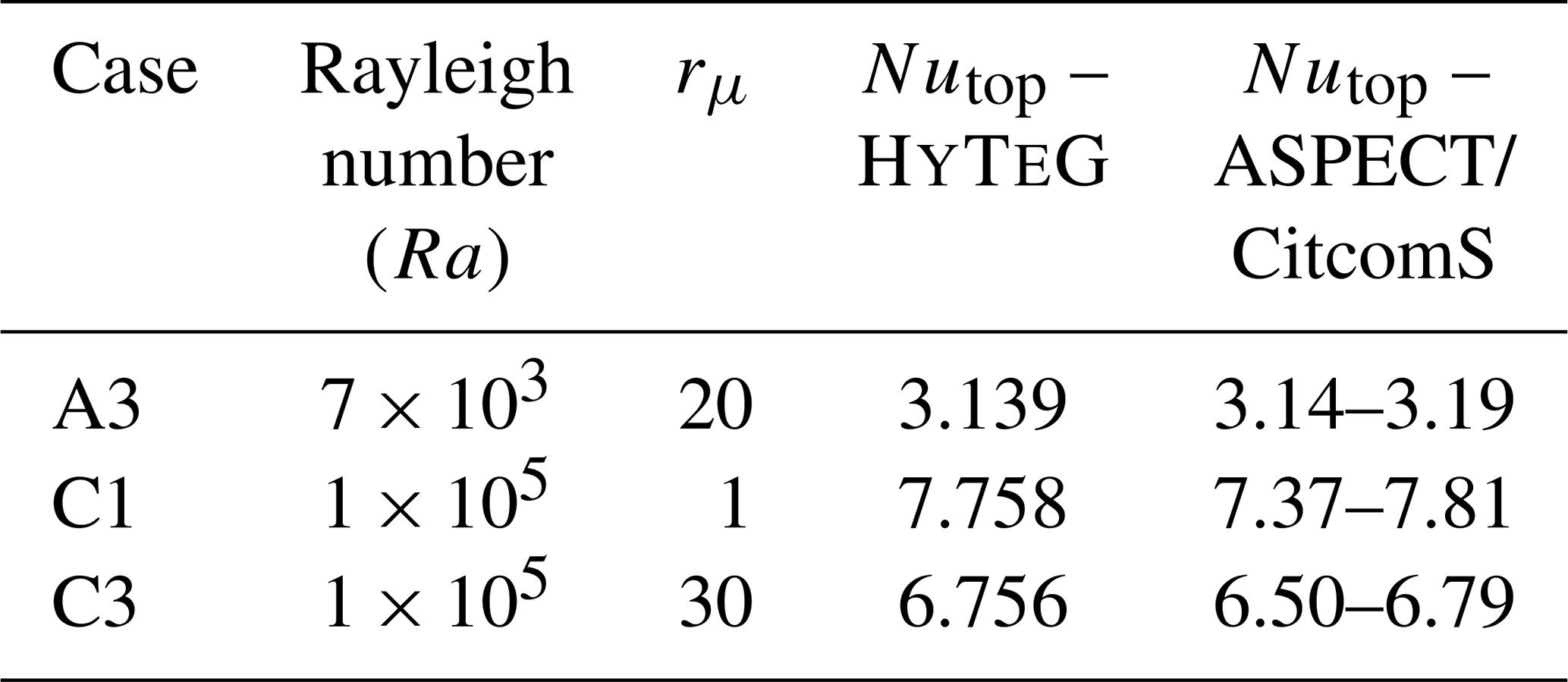
Fixing again the terms on the right-hand side and taking (∇T_h⋅n) to be an unknown FE function (∇T⋅n)_h living on ∂Ω it can also be obtained by solving a system with a boundary mass matrix. This is the approach we employed for computing the Nusselt numbers reported in Table 1.

Table 1 Test cases considered for comparison of Nusselt numbers (Nu) and radially averaged temperatures and velocity RMS values with published data from other codes (Euen et al., 2023).

4 Benchmarking and validation

In this section, we benchmark HyTeG against various geophysical problems. Initially, we consider mathematical convergence studies against analytical solutions of the Stokes problem on the thick spherical shell. We then move to time-dependent community benchmarks including setups with compressible flow, temperature-dependent and nonlinear rheologies. This is a continuation of the work done in Ilangovan et al. (2024) where several simple benchmark experiments had been conducted with HyTeG.

4.1 Stationary benchmarks

A common approach to verify numerical algorithms and their implementation is based on the method of manufactured solutions (Roache, 2001), which can be employed to check the order of convergence of the FE approximation to a known solution. However, this is typically restricted to comparatively simple setups and not actual application scenarios which usually involve complications such as e.g. discontinuities (or sharp variations) of material parameters. For incompressible Stokes flow on the annulus and spherical shell (semi-)analytical solutions were derived in e.g. Blinova et al. (2016), Horbach et al. (2019) and Kramer et al. (2021). In a similar vein, solutions based on the propagator matrix method were used in Zhong et al. (2000, 2008), Choblet et al. (2007) and Tan et al. (2011) to benchmark mantle convection frameworks. In Sect. 4.1.1 we first study HyTeG subject to the setup from Kramer et al. (2021), where the authors derive solutions for cases where the forcing function is in the form of a spherical harmonic and the same imposed with a Dirac delta function. To keep the setup closer to geodynamic models similar to Colli et al. (2018) and Brown et al. (2022) (where Dirichlet boundary conditions are considered on the outer surface), the boundary conditions chosen here are of mixed type (noslip on the outer boundary, free-slip on the inner boundary). As a baseline to evaluate the δ-function case we consider the mixed case boundary condition setup with a smooth forcing function. In addition, we also show the order of convergence of the computed radial stress on the free-slip boundary with respect to the analytical solution for the smooth forcing, mixed boundary condition case. Here, we compare the accuracy of the radial stress computed with an ℒ₂ projection of the gradient to the CBF method. We conclude this subsection by showing topography kernels computed at the surface and CMB for free-slip conditions. These kernels describe the response when placing a spherical density anomaly given by a specific spherical harmonic at various depths in the mantle. Next, in Sect. 4.1.2, we demonstrate convergence for the pure free-slip case when using the penalty approach to treat rigid body modes proposed in Sect. 3.4. For this we consider again the smooth forcing function.

4.1.1 Smooth and δ-function forcing

Consider the incompressible, isoviscous Stokes system

$$\begin{array}{}\text{(24)}& {\displaystyle }& {\displaystyle }-\mathrm{\nabla }\cdot \left(\mathrm{\nabla }\mathit{u}+(\mathrm{\nabla }\mathit{u}{)}^{\top }\right)+\mathrm{\nabla }p=f\mathit{g},\text{(25)}& {\displaystyle }& {\displaystyle }\mathrm{\nabla }\cdot \mathit{u}=\mathrm{0}\end{array}$$

posed on a thick spherical shell with r_min=1.22 and r_max=2.22. The radii are chosen such that we keep the aspect ratio of the domain close to that of Earth's mantle $\frac{r_{\min }}{r_{\max }}\simeq \mathrm{0.55}$ while having a unit thickness. We impose the no-slip conditions on the outer and free-slip on the inner boundary. The forcing functions f_δ and f_smooth are given by

$$\begin{array}{}\text{(26)}& f_{\mathrm{smooth}}={\displaystyle \frac{r^k}{R_{\max }^k}}{\mathcal{Y}}_{\mathrm{\ell }m}(\mathit{\theta },\mathit{\varphi }),f_{\mathit{\delta }}=\mathit{\delta }\left(r-r_{\mathrm{d}}\right){\mathcal{Y}}_{\mathrm{\ell }m}(\mathit{\theta },\mathit{\varphi }),\end{array}$$

where 𝒴_ℓm is the spherical harmonic function of order ℓ degree m, and δ(⋅) denotes the Dirac delta function. The analytical solution for the δ-function case will be a radial function piecewise defined on the two branches r<r_d and r>r_d, whilst satisfying an appropriate interface condition. Based on Kramer et al. (2021) we derived the analytical solution for the mixed boundary case in Ilangovan et al. (2024) and found the expected convergence orders for a P₂–P₁ pairing. Here we repeat this test using this time the FGMRES solver preconditioned with geometric multigrid described in Sect. 3.3. The coarse base mesh 𝒯₀ uses $(n_{\mathrm{rad}},n_{\tan })=(\mathrm{5},\mathrm{3})$ resulting in 486 nodes and 1920 tetrahedrons. Its radial layers are placed at the outer and inner surface and the middle one at r_d=1.72, where we center the δ-function.

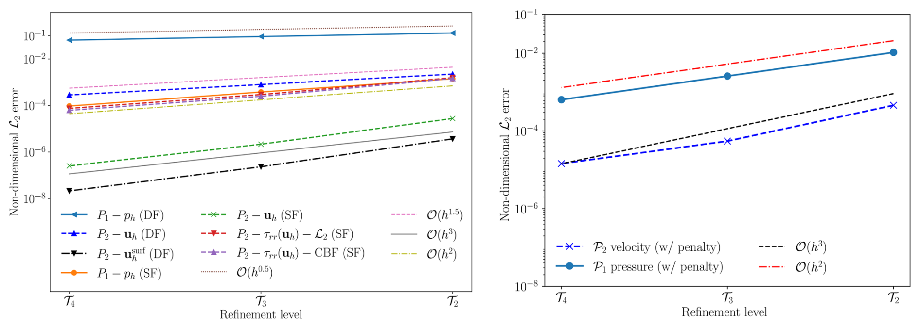
Figure 1 Left panel: order of convergence of the P₂–P₁ FE solution to analytical solution on the Spherical Shell with noslip condition on outer and free-slip on the inner surface (mixed case) under the δ-forcing (denoted by DF) function case and smooth-forcing (denoted by SF) function case for (ℓ=2, m=2, for SF case k=2); right panel: order of convergence of the P₂–P₁ FE solution to analytical solution on the Spherical Shell with free-slip imposed on both surfaces under the smooth forcing case and tuned rotational mode penalty for (ℓ=2, m=2, k=2).

Exploiting the definition of the δ-function the volume integral on the RHS of the discrete weak form reduces to a surface integral over of spherical layer at the corresponding depth r_d

$$\begin{array}{}\text{(27)}& \underset{\mathrm{\Omega }}{\int }\mathit{\delta }\left(r-r_{\mathrm{d}}\right){\mathcal{Y}}_{\mathrm{\ell }m}{\mathit{\varphi }}_i\mathit{g}\mathrm{d}\mathrm{\Omega }=\underset{{\mathrm{\Gamma }}_{r_{\mathrm{d}}}}{\int }{\mathcal{Y}}_{\mathrm{\ell }m}{\mathit{\varphi }}_i\mathit{g}\mathrm{d}\mathrm{\Gamma }.\end{array}$$

We study convergence going from 𝒯₂ (545 400 DoFs for velocity and pressure) up to 𝒯₄ (33 300 936 DoFs). The coarsest level for the multigrid solver is always set to 𝒯₂. The ℒ₂ error (e) on the domain Ω between the FE solution ${\mathit{u}}_h^{\mathrm{FE}}$ and the analytical solution ${\mathit{u}}_h^{\mathrm{analytical}}$ evaluated on the nodes of the FE mesh is computed as,

$$\begin{array}{}\text{(28)}& e=\sqrt{\left(\underset{\mathrm{\Omega }}{\int }\Vert {\mathit{u}}_h^{\mathrm{FE}}-{\mathit{u}}_h^{\mathrm{analytical}}{\Vert }_{\mathrm{2}}^{\mathrm{2}}\mathrm{d}\mathrm{\Omega }\right)}.\end{array}$$

The behaviour of the error, shown in Fig. 1 (left panel), demonstrates that the FE solution converges to the actual analytical solution with 𝒪(h³) for velocity and 𝒪(h²) for pressure in the case of smooth forcing (denoted by SF). This is the theoretically expected order of convergence for a P₂–P₁ Taylor Hood element. In addition, Fig. 1 (left panel) compares the errors in the radial stress computed on the inner free-slip boundary for the SF case, when using the ℒ₂-projection approach and the CBF method. Both achieve approximately a convergence order of 𝒪(h²). However, the overall error with the CBF method is consistently lower showing its superiority.

In the δ-function forcing case (denoted by DF), convergence of both the velocity and pressure solution deteriorates to 𝒪(h^1.5) and 𝒪(h^0.5) respectively, as can be seen from Fig. 1 (left panel). This is a known phenomenon, when considering the error over the complete domain, and can, supposedly, be attributed to the fact that, while the analytical pressure solution is discontinuous, we force it to be continuous by representing it as a P₁ function. However, when only considering the error on the free-slip surface one observes an 𝒪(h³) convergence of velocity for r_d in the interior. See Kramer et al. (2021) for a more detailed discussion.

As a final result, we present in Fig. 2 dynamic topography kernels for the surface and CMB. These are the responses resulting from spherical density perturbations placed at varying depths in the mantle. These perturbations are modeled again by f_δ from Eq. (26). Radial stresses are computed from the resulting velocity field using the CBF method and are used to extract the spherical harmonic coefficient corresponding to the spherical harmonic (ℓ, m). Extracting this value for every depth, gives the surface and CMB kernel functions for that spherical harmonic (ℓ, m). These are plotted in Fig. 2, where the kernel functions derived from the FE solution are overlaid with the ones derived from the analytical radial stresses on the same surface grid. The test uses the parameter set $(\mathrm{\ell },m)=\mathit{\left\{}\right(\mathrm{2},\mathrm{2}),(\mathrm{5},\mathrm{4}),(\mathrm{8},\mathrm{4}),(\mathrm{12},\mathrm{8}),(\mathrm{15},\mathrm{8}\left)\mathit{\right\}}$, although the kernels are only dependent on the degree ℓ (Ribe, 2007). From the plots, we see excellent agreement in the values from spherical harmonic degrees ℓ=2 to ℓ=15.

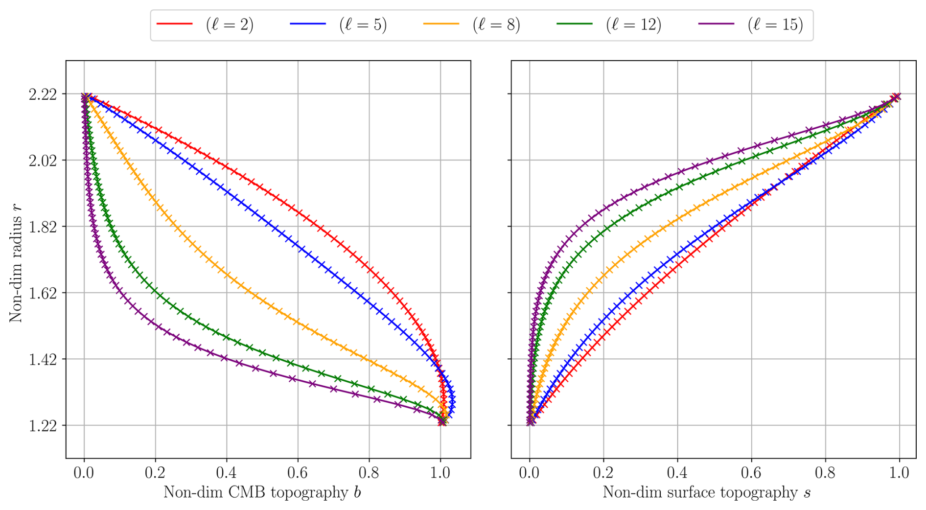
Figure 2 Kernels for the response of the surface and CMB topography to a δ-function forcing of the specified spherical harmonic degree (ℓ) placed at various depths in the mantle; solid lines denote the analytical solution and the cross marks (x) denote the FE computed solution.

4.1.2 Rotational mode penalty

In this part we focus on the convergence of the penalty approach described in Sect. 3.4 for the case of free-slip boundary conditions imposed on both the inner and outer surface. For this we prescribe a smooth forcing function (Eq. 26) for the Stokes system. We use the same domain configuration as in the previous section and also keep the multigrid preconditioned FGMRES solver. Again we study convergence going from 𝒯₂ up to 𝒯₄, while using 𝒯₂ as coarsest level for multigrid. The number of FGMRES iterations is kept the same at every refinement level 𝒯_l.

In Fig. 1 (right panel) we give errors with respect to an analytic solution without rigid body modes in the velocity field. The results demonstrate that choosing appropriate values for the penalty parameter maintains the expected O(h³) and O(h²) convergence for velocity and pressure, while taking care of the rigid body modes.

A theoretical study of the choice of penalty value is out of the scope of this contribution. Thus, the values for c_rot were tuned manually and set roughly to behave as O(h). Also to get this convergence behaviour, a different mesh configuration was chosen for 𝒯₀. The precise values for both can be found in the Python notebooks, see Ilangovan (2025).

4.2 Geophysical benchmarks

In this section, we will consider numerical convection experiments that are commonly used in the geophysics community to benchmark mantle convection frameworks. We start in Sect. 4.2.1 with a compressible convection simulation using the TALA approximation on a unit square. We test the approximation techniques proposed in Sect. 2.3.1 and 2.3.2 and verify the resulting Nusselt number against other codes. Then in Sect. 4.2.2, we perform the benchmark from Tosi et al. (2015) which employs a viscoplastic rheology. Finally, in Sect. 4.2.3, we consider the benchmark from Ratcliff et al. (1996) and Zhong et al. (2008) on the spherical shell and compare the radially averaged temperatures and Rayleigh number vs. Nusselt number trends reported in other works.

4.2.1 Compressible case

We consider the compressible Stokes equations (Eqs. 5 and 6) coupled with the energy equation (Eq. 8) on the unit square. The goal is to perform an experiment using our methodologies with the setup being identical to that in King et al. (2010) and compare the Nusselt numbers that we obtain on the top boundary. In the benchmark free-slip boundary conditions are imposed on all sides. In addition to diffusion and adiabatic heating/cooling in the energy equation (Eq. 8), we also include the shear heating term. The experiment is started from an initial sinusoidal perturbation,

$$\begin{array}{}\text{(29)}& T(\mathbf{x},t=\mathrm{0})=(\mathrm{1}-y)+A_{\mathrm{0}}\cos \mathit{\pi }x\sin \mathit{\pi }y,\end{array}$$

with A₀=0.1, which then induces a single convection cell in the square.

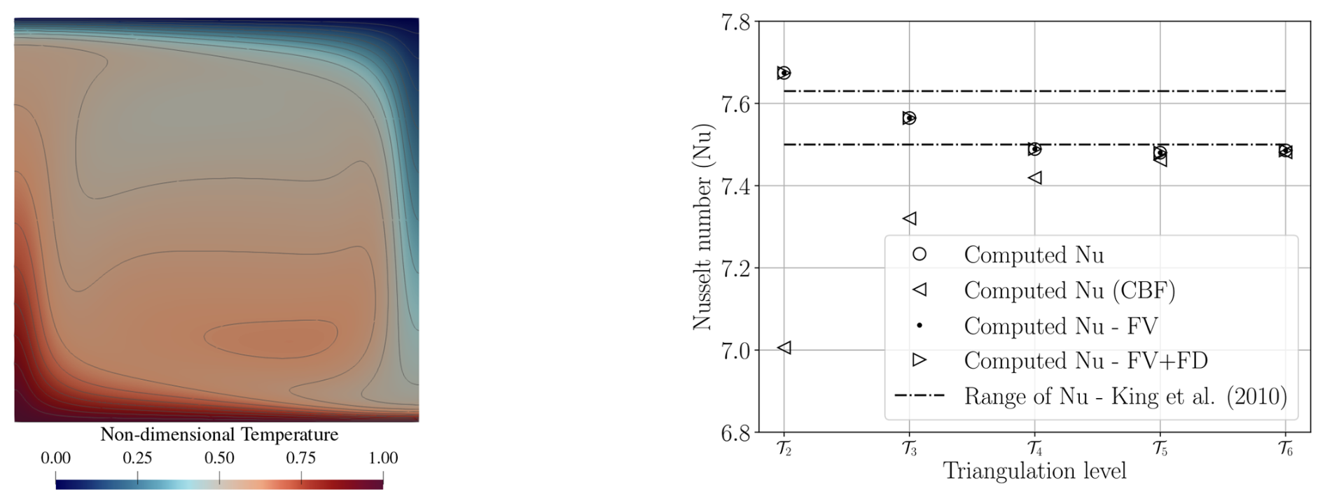
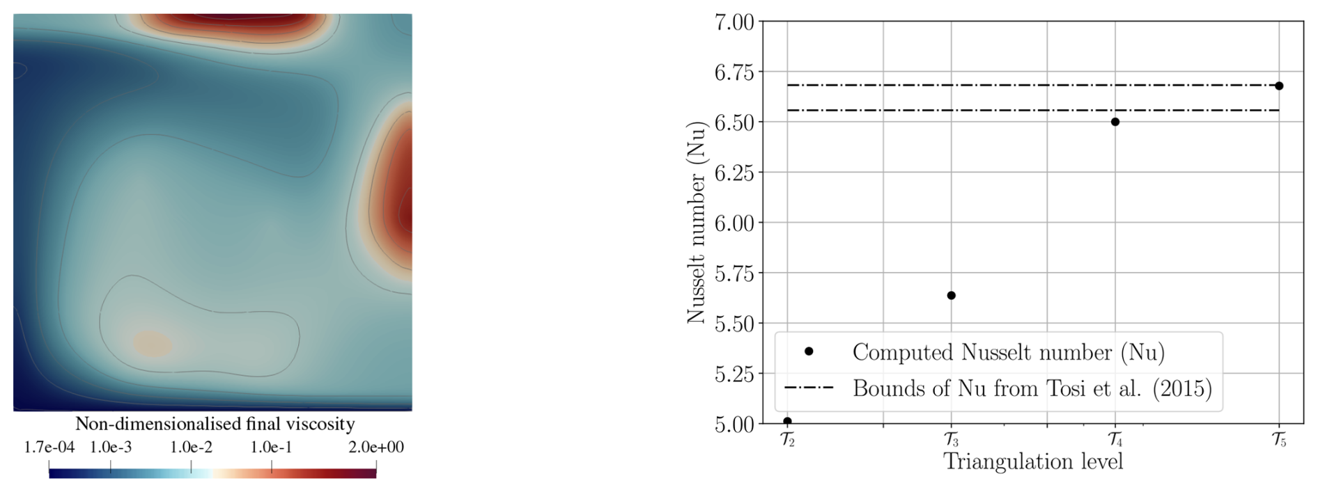
Figure 3 Left panel: final temperature contours of the compressible benchmark on an unit square of the TALA case from King et al. (2010) presented in Sect. 4.2.1 with Ra=10⁵ and Di=0.5; right panel: comparison of Nusselt number values between the Frozen velocity approach (FV, see Sect. 2.3.1) and including Frozen divergence approach (FD, see Sect. 2.3.2) under the setup from Sect. 4.2.1 identical to the TALA case from King et al. (2010) at Ra=10⁵ and Di=0.5.

An isoviscous, compressible case with $\stackrel{\mathrm{‾}}{\mathit{\rho }}=\exp \left[Di\right(\mathrm{1}-y\left)\right]$ is considered, where Di is the dissipation number taken as Di=0.5. The unit square mesh contains 4 subdivisions in the x and y direction generating a total of 32 triangles at the coarsest level 𝒯₀. The triangles are refined to reach the operating mesh at level n denoted as 𝒯_n. To solve the linear system of equations the FGMRES solver with multigrid as preconditioner is used. The finest level for the multigrid is 𝒯_n and the coarsest level 𝒯₀. Time-steps are calculated based on the CFL condition. At each time-step, 10 iterations are performed with the FGMRES solver, with two coupling Picard iterations between the Stokes and energy equation. The system (Eqs. 5, 6 and 8) is non-dimensionalised following King et al. (2010), which introduces the Rayleigh and Dissipation number. The simulation is performed at Rayleigh number Ra=10⁵ and run until the temperature reaches a steady state as seen in Fig. 3. After this, the Nusselt number is computed on the top boundary and checked for convergence. The Nusselt number describes the ratio between heat transported by convection to heat transported purely by diffusion. Taking the pure diffusion solution as reference, T_ref, the Nusselt number can, thus, be computed for the final temperature solution T via

$$\begin{array}{}\text{(30)}& Nu={\displaystyle \frac{\underset{\mathrm{\Gamma }}{\int }\mathrm{\nabla }T\cdot \widehat{\mathbf{n}}\mathrm{d}\mathrm{\Gamma }}{\underset{\mathrm{\Gamma }}{\int }\mathrm{\nabla }{T}_{\mathrm{ref}}\cdot \widehat{\mathbf{n}}\mathrm{d}\mathrm{\Gamma }}}.\end{array}$$

We compare three different approaches for the compressible setting here. Using the full asymmetric Stokes system, employing the frozen velocity approach (from Sect. 2.3.1) and additionally also the frozen divergence approach (from Sect. 2.3.2). The corresponding Nusselt numbers are reported in Fig. 3 (right panel). From the figure we can see that all three approaches behave very similarly and converge to the same Nusselt number. Note that this final value is on the lower end of the Nusselt numbers reported in King et al. (2010) (Nu=7.50). Specifically this is the value for the CZ code, which also uses a semi-Lagrangian approach to treat advection. Hence, as our approach is also similar to this, the Nusselt numbers computed here are expected.

Note that the temparature gradient in Eq. (30) appears in the integrand. It can, thus, be evaluated and used locally, without resorting to the methods discussed in Sect. 3.5, as we have done here. For comparison, we also computed Nu for the asymmetric approach using the CBF method. As can be seen it approaches the same final value albeit from below.

4.2.2 Nonlinear rheology

Although the rheology of the mantle is not completely known, it is clear that it exhibits a nonlinearity (Cordier and Goryaeva, 2018). A simple example would be plate boundaries, where large stresses (which depend on the velocity u) make the plates exhibit plastic behaviour. This decreases viscosities giving rise to weak zones at these locations. In this section, we conduct a plume rising experiment with a sinusoidal temperature perturbation (Eq. 29) on the unit square with a nonlinear rheology. The setup is identical to case 4 from Tosi et al. (2015), where the viscosity is defined as

$$\begin{array}{}\text{(31)}& {\displaystyle }& {\displaystyle }\mathit{\mu }={\left({\displaystyle \frac{\mathrm{1}}{{\mathit{\mu }}_{\mathrm{linear}}}}+{\displaystyle \frac{\mathrm{1}}{{\mathit{\mu }}_{\mathrm{nonlinear}}}}\right)}^{-\mathrm{1}}\text{(32)}& {\displaystyle }& {\displaystyle }{\mathit{\mu }}_{\mathrm{linear}}=\exp \left(-{\mathit{\gamma }}_{T}T+{\mathit{\gamma }}_{z}z\right)\text{(33)}& {\displaystyle }& {\displaystyle }{\mathit{\mu }}_{\mathrm{nonlinear}}={\mathit{\mu }}^{*}+{\displaystyle \frac{{\mathit{\sigma }}_y}{\sqrt{\dot{\mathit{ϵ}}:\dot{\mathit{ϵ}}}}}.\end{array}$$

Here γ_T and γ_z are positive constants, and the constant μ^* models the effective viscosity in the nonlinear regime, which is active when the stresses exceed the yield stress σ_y. We treat the viscosities as a P₀ FE function, i.e. constant per cell, and average them on coarser grids. The FGMRES solver with a multigrid preconditioner applied to the viscous A-Block is used with 10 FGMRES iterations per Stokes solve. We run the simulation until a single convection cell has stabilised in the domain. The dependence of viscosity on velocity makes the Stokes system nonlinear, which we handle by performing five Picard type iterations at every time-step. This number could be reduced, though, once the system starts to stabilise. The final viscosity contour in log scale can be seen from Fig. 4 (left panel). If viscosity was only temperature-dependent (μ_linear), then it would consistently be large along the top and right boundary of the domain, where temperature is coldest. However, as we consider a pseudoplastic rheology, the viscosity is considerably smaller where stress is large. This is the case in the upper left and right boundary, where rising material hits the top or starts sinking down, but also at the lower part of the right boundary. Figure 4 (right panel) shows the resulting Nusselt number at the top boundary and how it behaves when we refine the mesh. For a high enough resolution the value falls inside the region reported for other codes in Tosi et al. (2015) and Davies et al. (2022).

Figure 4 Results for the setup described in Sect. 4.2.2 after reaching steady state: left panel: final viscosity contours showing formed weak zones; right panel: convergence of the Nusselt numbers computed on the top boundary with mesh refinement.

4.2.3 Spherical shell

This section involves experiments on a thick spherical shell where an incompressible Stokes system with variable viscosity coupled to an energy equation is considered (Ratcliff et al., 1996; Zhong et al., 2008; Davies et al., 2022; Euen et al., 2023). The boundary conditions prescribed are of free-slip type on both inner and outer surface. The initial condition for the temperature field is a radially linear function with an added symmetrical perturbation according to a spherical harmonic function 𝒴_lm. The benchmark consists in checking, if the spherical harmonic components of the resulting temperature field largely maintain the prescribed order and degree. The initial condition for the temperature field is given by

$$\begin{array}{}\text{(34)}& T(t=\mathrm{0})=T_{\mathrm{ref}}+\mathit{ϵ}{T}_{\mathrm{perturb}},\end{array}$$

with ϵ>0. T_ref is a reference profile which satisfies the steady diffusion equation. We consider two types perturbations T_perturb=𝒴_ℓm: a choice of degree ℓ=3 and order m=2 results in a tetrahedral symmetry of plumes and downwellings, while a cubic symmetry is obtained for $T_{\mathrm{perturb}}={\mathcal{Y}}_{\mathrm{40}}+\frac{\mathrm{5}}{\mathrm{7}}{\mathcal{Y}}_{\mathrm{44}}$. The prescribed viscosity variation is dependent on the evolving temperatures and is given by the following expression,

$$\begin{array}{}\text{(35)}& \mathit{\mu }={\mathrm{10}}^{r_{\mathit{\mu }}\left(\frac{\mathrm{1}}{\mathrm{2}}-T\right)},\end{array}$$

where r_μ>0 and T is the non-dimensional temperature whose values lie between 0 and 1. By increasing the value of r_μ, the viscosity contrast between the plumes and downwellings can be increased. By taking a pure diffusion solution as the reference, $T_{\mathrm{ref}}=\frac{r_{\min }{r}_{\max }}{r}-r_{\min }$, the Nusselt number can be computed with Eq. (30). Experiments are performed on a thick spherical shell with r_min=1.22 and r_max=2.22, which has an aspect ratio of $\frac{r_{\min }}{r_{\max }}\simeq \mathrm{0.55}$, which is similar to that of Earth's mantle, while keeping non-dimensionalised thickness of 1 (Ratcliff et al., 1996; Davies et al., 2022).

The Stokes system is solved with the geometric multigrid preconditioned FGMRES solver described in Sect. 3.3. Simulations are started with 25 FGMRES steps for the first 25 time-steps. Afterwards the number of FGMRES iterations is reduced to between 5 and 15 depending on the magnitude of viscosity contrasts (15 when r_μ>10²). On each multigrid level three pre- and postsmoothing steps with a 3rd order Chebyshev smoother are applied. MINRES is used as the coarse grid solver. The coarsest level (𝒯₂) of the multigrid solver corresponds to a resolution of $(n_{\tan },n_{\mathrm{rad}})=(\mathrm{9},\mathrm{5})$ and the finest level (𝒯₄) to (33, 17). For comparison to other published results, we consider the scenarios A3, C1, and C3 from Zhong et al. (2008), also presented in Euen et al. (2023), for which the respective values used can be seen from Table 1. We then also simulate the A7 case from Zhong et al. (2008) to assess the regime switching point.

In addition, we perform multiple simulations and plot the variation of the Nusselt number with respect to the Rayleigh number as was done in Ratcliff et al. (1996).

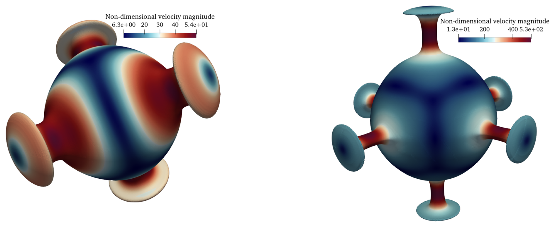
Figure 5 Left panel: temperature isosurfaces at T=0.5 for the A3 case coloured with non-dimensional velocity magnitudes; right panel: temperature isosurfaces at T=0.5 for the C3 case coloured with non-dimensional velocity magnitudes.

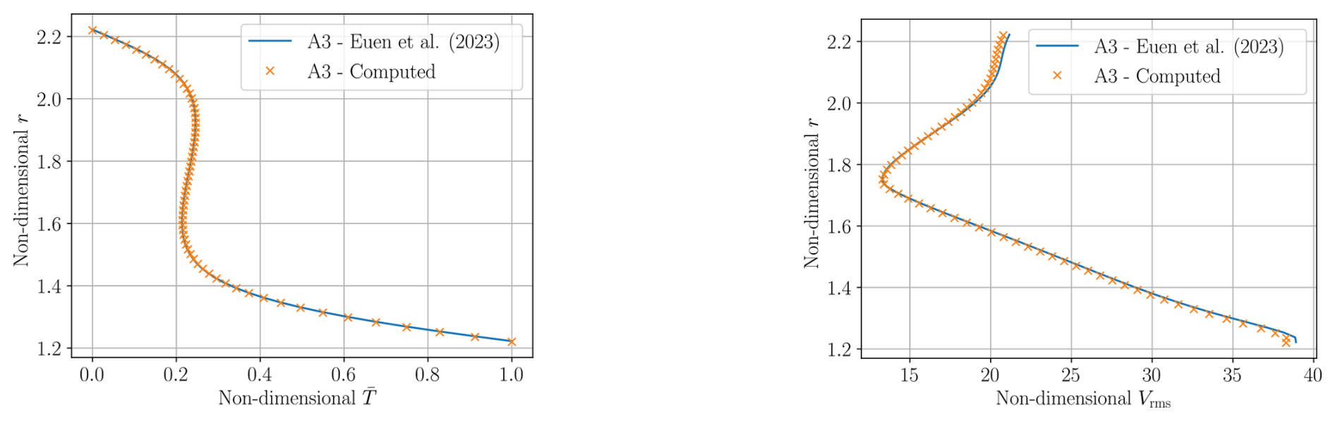
Figure 6 Radially averaged temperature values $\stackrel{\mathrm{‾}}{T}$ (left panel) and radially averaged velocity RMS values V_rms (right panel) for the A3 case from Zhong et al. (2008); we compare the results published in Euen et al. (2023) (solid line) with results computed in our setup.

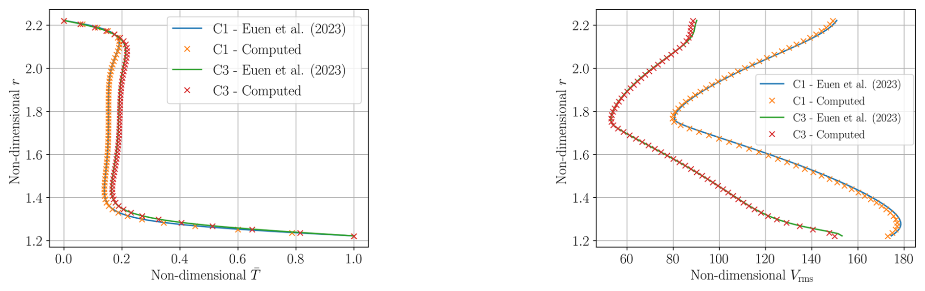
Figure 7 Radially averaged temperature values $\stackrel{\mathrm{‾}}{T}$ (left panel) and radially averaged velocity RMS values V_rms (right panel) for the C1 and C3 cases from Zhong et al. (2008); we compare the results published in Euen et al. (2023) (solid lines) with results computed in our setup.

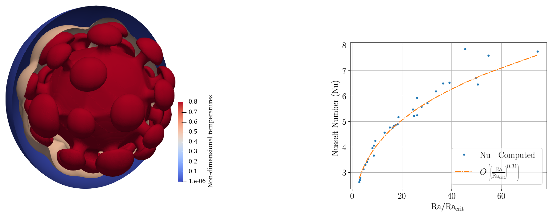
Figure 8 Left panel: temperature isosurfaces at T=0.8 (red), T=0.5 (light red) and $T={\mathrm{10}}^{-\mathrm{6}}$ (blue) for the A7 case from Zhong et al. (2008); right panel: variation of Nu vs. ($Ra/R{a}_{\mathrm{crit}}$) for the cubic symmetry case; each data point denotes a simulation run where Ra_crit is computed depending on the r_μ value for a given spherical harmonic perturbation, with the best fit exponent plotted side by side $(Ra/R{a}_{\mathrm{crit}}{)}^{\mathrm{0.31}}$.

All simulations are run until the system reaches a statistical steady state i.e. the radially averaged temperatures and the Nusselt numbers converge to a certain value. A CFL condition threshold (see Eq. 13) of C_CFL=1.2 is used, which we gradually increased to C_CFL=1.5 when we approach the steady state. The resulting temperature isosurfaces at T=0.5 coloured by the magnitude of velocity are given in Fig. 5 for the A3 and C3 case. The radially averaged temperatures and velocity RMS values from the final time-step are plotted for our simulations in combination with the data presented in Euen et al. (2023) for the A3 case in Fig. 6 and the C1 and C3 case in Fig. 7. The corresponding Nusselt numbers are presented in Table 1. The radius values from Euen et al. (2023) are scaled $\left(\times \frac{\mathrm{1}}{\mathrm{0.45}}\right)$ for comparison with the results computed here as the mantle thickness is different in both setups, although they are comparable since the aspect ratio of the domain is the same in both setups. As can be seen from the figures, the results obtained with our framework agree well with those presented in Euen et al. (2023) for ASPECT and CitComS.

Results for scenario A7 are given in the left of Fig. 8. Here one keeps the Rayleigh number at $Ra=\mathrm{7}\times {\mathrm{10}}^{\mathrm{3}}$, but increases r_μ to 10⁵. This takes us past the transition point from a steady state regime to a stagnant lid regime. The viscosity contrast is now so high that viscosity increases drastically towards the outer surface preventing the development of downwellings there. Also, plumes are restricted to the lower region near the inner surface.

Next we consider multiple cases with different Rayleigh numbers and r_μ values to analyse the variation of the achieved Nusselt number with respect to Rayleigh numbers. For a given r_μ value and a given degree ℓ of spherical harmonic perturbation T_perturb=𝒴_ℓm, there exists a specific value Ra_crit, that indicates the onset of convection, see the stability analysis in Zebib (1993). Specifically we consider all combinations of Rayleigh numbers $Ra\in \mathit{\{}\mathrm{7}\times {\mathrm{10}}^{\mathrm{3}},\mathrm{2}\times {\mathrm{10}}^{\mathrm{4}},\mathrm{4}\times {\mathrm{10}}^{\mathrm{4}},\mathrm{6}\times {\mathrm{10}}^{\mathrm{4}}\mathit{\}}$ and $r_{\mathit{\mu }}\in \mathit{\{}\mathrm{3},\mathrm{10},\mathrm{20},\mathrm{40},\mathrm{100},\mathrm{500},\mathrm{700},\mathrm{1000}\mathit{\}}$ for the case of the perturbation with cubic symmetry (giving us degree ℓ=4). The choice of values is motivated by Ratcliff et al. (1996). For each combination we perform one simulation run with a CFL threshold of 1.2 and compute the Nusselt number at the end of the simulation. These are then plotted in Fig. 8 (right panel) versus $\frac{Ra}{R{a}_{\mathrm{crit}}}$, where the critical Rayleigh number was taken from Zebib (1993). As can be seen, a power law exponent of 0.31 fits the Nusselt number data well, which is in accordance with earlier studies (Jarvis, 1993). Although these experiments are a challenging test to the framework, we see that the benchmarks only compare the steady state result reached at the end of the simulation, while there is nothing that can be said about how the Stokes and Energy solver gets there. As the result is only verified at the end of the time evolution, the temperature and velocity patterns through which the solvers reach the solution can be different.

5 Scalability of the framework

Development of the HyTeG framework is performed with a focus on HPC applications at the extreme scale. Thus, scalability studies have already been presented, e.g. in Kohl and Rüde (2022) and Böhm et al. (2025). These were, however, either limited to simple (isoviscous) Stokes problems or other operators such as curl-curl.

In order to highlight the capabilities of our state-of-the-art framework when running high-resolution global-scale mantle convection models, we consider in this section its scaling behaviour for a realistic model with varying viscosity and mixed boundary conditions posed on a thick spherical shell. Since the major chunk of the computational effort goes into solving the Stokes system, Eqs. (5) and (6), we focus on the latter for our experiments.

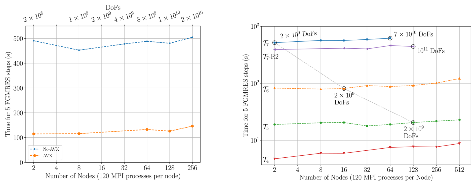
Figure 9 Left panel: weak scaling at 𝒯₆ for an identical setup with and without vectorization using the code generated from the HOG generator, right panel: weak scaling behaviour on the Hawk supercomputer at HLRS (66th on Top500 as of November 2024) up to 512 nodes; 𝒯₄, 𝒯₅, 𝒯₆ or 𝒯₇ gives the highest refinement level when simulating the variable viscosity Stokes system; the postfix-R2 indicates a weak scaling test with peak number of unknowns being 10¹¹ (but a restart of FGMRES after already two steps due to memory limitations).

As before we again use block preconditioned FGMRES with geometric multigrid for the A-block as solver, see Sect. 3.3. Experiments were performed on the Hawk supercomputer at HLRS (66th on the Top500 list as of November 2024). We demonstrate scalability with up to approximately 10¹¹ DoFs on 15 360 cores. The timings reported are for 5 FGMRES steps with a restart at every 3 steps and 1 pre- and post-smoothing iteration each per level in the multigrid solver. For a single weak scaling test, we fix the number of coarse mesh elements to 1 per MPI process and refine it several times as outlined in Sect. 2.1. Keeping the maximal refinement level fixed, while increasing the number of processes, then maintains the number of DoFs per process. We perform multiple weak scaling tests at different refinement levels 𝒯_k.

We first present in Fig. 9 (left panel) a comparison between the runtime of the application compiled once with and once without vectorization. As can be seen from the plot, we achieve nearly a 4x improvement with the HOG-generated kernels supporting AVX extensions (Böhm et al., 2025), and the following results also use this optimisation.

In the runtimes reported in Fig. 9 (right panel), we consider multiple weak scaling cases. Each line indicates a single weak scaling test and the 𝒯_k next to the line denotes the highest level (k) of refinement the corresponding test was performed at. From the plots, we see that the framework scales extremely well for up to 61 440 MPI processes. The slightly reduced runtime for the 𝒯₆ case in the right figure stems from a technical change with respect to the implementation of the treatment of free-slip boundary conditions, see Sect. 2.1. This change applies to all our weak scaling runs. These also used a representation of viscosity as P₁ function. This, however, had no significant influence on the runtime behaviour.

To further test the capabilities of TerraNeo we increased the number of DoFs to about 10¹¹ and simulated a variable viscosity Stokes system on 15 360 cores. Due to memory limitations we needed to adjust the solver setup and restarted FMGRES already after 2 steps. The results are marked by -R2 in Fig. 9 and demonstrate that the code can also handle a system of this size.

With respect to the strong scaling behaviour of the framework, we highlight in Fig. 9 (right) three runs using the same problem size, i.e. 2×10⁹ DoFs, but different number of MPI processes and, thus, also different refinement levels. The system when solved at 𝒯₇ on 2 nodes takes about 500 s, while it can be brought down to ≃20 se on 128 nodes at refinement level 𝒯₅. These results clearly show that the framework is scalable and suitable for handling globally resolved mantle convection models.

An important point to note is that, these tests only assess the Stokes solver for the scalability of its implementation in HyTeG and not on its solvability to achieve a specific residual reduction.

6 Conclusions

In this paper, we presented a comprehensive evaluation of the HyTeG Finite Element framework when applied to problems from computational geodynamics. We assessed the key components required for large-scale mantle convection simulations, including the multigrid-based linear solver for the Stokes system and a semi-Lagrangian advection scheme, through a series of targeted tests and geophysical benchmarks.

We verified the expected convergence rates of the Finite Element solutions against analytical results for Stokes flow with Dirac-delta-type forcing, demonstrating the robustness of the implemented multigrid solver. We also proposed and validated a novel methodology to eliminate rigid body modes in the thick spherical shell geometry with tangential stress-free, no-normal-flow boundary conditions.

We conducted benchmark simulations representative of realistic geodynamic scenarios, including compressible flows and nonlinear, temperature-dependent rheologies. These experiments spanned from unit square domains to thick spherical shells and confirmed the physical fidelity and numerical stability of the proposed methods.

Scalability studies on the Hawk supercomputer (ranked 66th on the Top500 list as of November 2024) showed that our implementation is capable of handling up to 10¹¹ degrees of freedom in the Stokes system. While the FGMRES solver exhibits robustness under large viscosity contrasts, the convergence is hindered by inadequate coarse-grid approximations in the geometric multigrid preconditioner. Addressing this bottleneck is an ongoing area of research, with continued exploration of techniques for improved coarse-level correction.

Overall, our results demonstrate that HyTeG is a highly scalable and capable framework for finely resolved mantle convection simulations. Future work will focus on further optimizing multigrid performance and exploring advanced solver strategies to fully exploit the potential of matrix-free methods at extreme scales.