
the Creative Commons Attribution 4.0 License.
the Creative Commons Attribution 4.0 License.
 | 20 Nov 2026
FluidUrban v1.0: enhancing urban ventilation and pollutant dispersion modelling with three-dimensional dynamic adaptive meshes optimisation

Siyang Chen
Jinxi Li
Yu Zhang
Zifa Wang
Pu Gan
Jie Zheng
Fangxin Fang
Simulating urban airflow and pollutant dispersion requires resolving multiscale physical processes, from large-scale meteorological forcing to highly localized building-induced turbulence. To accurately capture these multiscale urban flow fields, this study introduces FluidUrban v1.0, an advanced modelling system built upon the Fluidity solver and centred on a three-dimensional Dynamic Adaptive Mesh Optimization (DAMO) framework. By dynamically adapting mesh resolution in response to the evolution of flow physics and scalar gradients, DAMO concentrates computational resources on critical high-gradient regions such as building wakes, shear layers and scalar sharp plumes. The model's performance is systematically evaluated against high-fidelity “WOTAN” wind-tunnel experimental data under varying surface roughness conditions and inflow directions. The results demonstrate that the FluidUrban with DAMO framework consistently outperforms traditional non-uniform fixed meshes (FIXM) by accurately capturing complex urban wind fields and pollutant concentration. For normalized wind speed, FluidUrban with DAMO achieved a Mean Absolute Error (MAE) of 0.187, representing a notable reduction from 0.214 simulated by FIXM. In terms of wind direction, the model reduced the MAE by up to 38.4 % in medium roughness and 36.1 % in high roughness conditions, respectively, during realistic oblique inflow scenarios. Additionally, DAMO effectively mitigates the non-physical numerical dissipation observed in static meshes, significantly improving the prediction of streamwise and lateral turbulence intensities. Furthermore, for pollutant dispersion, the model effectively suppressed numerical diffusion and maintained sharp plume gradients, achieving an 89 % compliance rate with established atmospheric model evaluation standards (FB, NMSE, and MG), compared to only 50 % for FIXM. Although DAMO introduces runtime overhead for mesh regeneration, this cost is justified by significant gains in physical accuracy and multi-scale flow resolution. Following the systematic evaluation, FluidUrban v1.0 was applied to a realistic urban scenario, demonstrating its robust capability to resolve the complex flow fields and spatial heterogeneity within real urban morphologies. Thus, FluidUrban v1.0 demonstrates to be a robust aerodynamic tool for resolving the transient, small-scale flow structures critical to pollutant transport, establishing a solid foundation for the future integration of comprehensive urban physical components, including radiation, vegetation, and full energy-balance physics.
- Article
(14904 KB) - Full-text XML
- BibTeX
- EndNote


Projections indicate that by 2050, over 70 % of the global population will reside in cities, with the growth of megacities expected to accelerate in the coming decades (United Nations, 2019). This rapid urbanization threatens to exceed urban carrying capacities, presenting substantial environmental, infrastructural, and social challenges. Among these, urban heat island and air pollution have become critical concerns with significant implications for human health and sustainable development (Connerton et al., 2020; Khomenko et al., 2021; Apte and Manchanda, 2024). The efficacy of urban heat and pollutant dispersion is directly linked to urban ventilation, which is shaped by the complex interaction between building morphology, city density, and local aerodynamic conditions (da Silva et al., 2021, Liang and Zheng, 2026). Accurately and quickly modelling these wind fields is therefore vital for designing sustainable residential environments and effective emission control strategies. However, capturing the multiscale nature of pollutant transport, driven by heterogeneous surface heating and complex urban geometries, requires high-resolution, physically consistent numerical simulations (Zhang et al., 2018; Nagai et al., 2021; Khan et al., 2025). As a result, advanced numerical modelling has emerged as an essential tool for evaluating ventilation potential and guiding urban atmospheric management (Badach et al., 2020; Khan et al., 2021; Liu et al., 2023).
With the rapid development of the computer hardware, Computational Fluid Dynamics (CFD) simulations are becoming an efficient and important method to conduct the study of urban wind fields and air pollutant dispersion (Hang et al., 2013; Mottet et al., 2020; Zhong et al., 2022; Kusaka et al., 2024), which output detailed information of 3D flow variables in the whole computational field and display them visually. However, modeling airflow and pollutant dispersion in urban areas is complicated by the tight coupling of multiscale physical processes (Di Sabatino et al., 2013). Large-scale meteorological forcing determines the prevailing wind, whereas small-scale interactions with building geometries induce complex vortex shedding and turbulence, which can significantly modify the mean flow field (Giani and Crippa, 2024). This creates an extra wide spatial spectrum to resolve: spanning from the planetary boundary layer that transports plumes over long distances, down to the inertial sub-range turbulence within street canyons that governs pedestrian-level exposure. Chemical aging of pollutants further complicates this, as emissions undergo rapid transformation immediately upon release from localized sources (e.g., smokestacks or roadways) before dispersing over the urban canopy (Weger and Heinold, 2023). Simulating a large city with a fixed grid fine enough to resolve individual building features is computationally infeasible. These methods often struggle to capture highly localised and transient dynamic processes, such as building-induced vortices and shear layers, as well as flow variations around building edges and within street canyons (Jackson et al., 2015; Pesci et al., 2018). To address this, conventional CFD approaches utilize nested or stretched meshes to statically refine specific regions of the domain (Park and Kim, 2024). However, such methods suffer from critical shortcomings: they impose nested boundaries that create artificial wave reflections at grid interfaces, introduce significant numerical diffusion as plumes drift into coarser zones, and waste computational resources by over-refining inactive regions where high resolution is unnecessary. Consequently, Three-Dimensional (3D) Dynamic Adaptive Mesh Optimization (DAMO), often implemented via Adaptive Mesh Refinement (AMR), offers the most viable path forward. By dynamically refining grid resolution in real-time response to flow physics (such as velocity) and scalar gradients (such as pollutant concentration), DAMO enables a unified modeling system (AMCG, 2014). This approach seamlessly couples scales, accurately capturing the non-linear feedback loops between regional meteorological forcing and local street-canyon turbulence without the computational cost of uniformly fine grids. By automatically refining and coarsening the mesh in response to solution features such as velocity gradients or vorticity, DAMO enables computational resources to be focused where they are most needed (Zheng et al., 2015; Sezen and Atlar, 2022; Yu et al., 2024). This technique has shown considerable potential for improving both accuracy and computational efficiency across a range of geophysical fluid applications, including boundary-layer dynamics (Bauer et al., 2020), cloud–aerosol interaction processes (Han et al., 2023), and atmospheric chemical transport mechanisms (Yang et al., 2025).
Although DAMO has demonstrated its potential to capture building wake dynamics and high-gradient pollutant structures (Zheng et al., 2021; Wu et al., 2023; Li et al., 2025), a critical need remains to transition generic adaptive solvers to dedicated urban multi-physics frameworks. To address this, this study introduces FluidUrban v1.0, a novel urban modeling framework centered on 3D DAMO. FluidUrban v1.0 is built upon the well-established open-source Fluidity solver (Imperial College London), which has proven robust in large-scale atmospheric advection and complex terrain simulations utilizing anisotropic adaptive unstructured meshes (Pain et al., 2005; Li et al., 2018). Building upon this mathematical foundation, FluidUrban v1.0 is specifically developed to adapt these advanced numerical techniques for high-resolution urban micrometeorology. By developing a dedicated 3D urban geometry and unstructured mesh generator, and coupling it with urban boundary conditions, the model serves as a foundational framework capable of resolving highly localized and transient dynamic processes, such as building-induced vortices and shear layers, that are often smoothed out by traditional approaches (Jackson et al., 2015; Pesci et al., 2018).
Concurrently, establishing the reliability of this newly developed framework requires systematic and quantitative evaluation. Much of the existing studies of DAMO simulation focus on qualitative visual improvements, leaving a critical gap in quantifying the specific gains in accuracy and computational efficiency that DAMO offers relative to fixed-mesh benchmarks (Zheng et al., 2015; Tarraf et al., 2024). To address these validation gaps, wind tunnel experiments (WTE) usually serve as the “ground truth” standard for benchmarking urban CFD models. Unlike field measurements, which are limited by uncontrollable meteorological variability and sparse sampling, WTE provides high-fidelity and controllable datasets ideal for isolating specific flow phenomena like cavity recirculation and street-canyon ventilation. While established databases like CEDVAL (Hamburg University) and the Architectural Institute of Japan (AIJ) guidelines remain the foundation for verifying mean flow and turbulence statistics (Tominaga et al., 2008; Ricci et al., 2017), recent work by Wang et al. (2025) demonstrates that validating adaptive models requires not just point-measurements, but dense and spatially-resolved data to capture the sharp gradients of pollutant plumes in the inertial sub-range. Furthermore, contemporary studies utilise these datasets to assess solver fidelity under complex transient conditions, such as gusty cross-canyon flows, which are often smoothed out by traditional RANS approaches but are critical for accurate exposure modelling (Gromke, 2011; Cui et al., 2016; Arafa and Zinat, 2025).
Thus, the primary objective of this study is to develop a novel urban modeling framework FluidUrban v1.0 centered on 3D DAMO and provide a comprehensive validation of the model against wind-tunnel experiments and standard fixed-mesh simulations, thereby quantifying the benefits of 3D adaptivity for urban flow and pollutant dispersion. The remainder of the paper is organised as follows: Sect. 2 details the model setup, focusing on the model development, the governing equations and implementation of the physics-driven DAMO algorithm. Section 3 presents a quantitative performance evaluation for both urban wind flows and pollutant dispersion, and analyses how the adaptive strategy captures key urban flow features. Section 4 shows the performances of the model used in a realistic urban scenario simulation. Finally, Sect. 5 summarises the principal conclusions and discusses its implications of this framework for next generation of urban environmental modelling.
2.1 Model development
FluidUrban v1.0 is built upon the open-source Fluidity solver. The core advancement of this new framework lies in the development of a dedicated generator of 3D urban geometry and unstructured meshes, which is subsequently coupled with urban-specific micrometeorological boundary conditions. This systematic integration enables the model to accurately initialize and dynamically resolve complex urban flow topologies.
2.1.1 Urban geometry and unstructured mesh generator
While DAMO optimises the meshes during runtime, generating an accurate geometry and initial mesh is a prerequisite to explicitly resolve the complex morphology and heterogeneous geometry of the realistic urban canopy. To achieve this, a dedicated 3D urban geometry and unstructured mesh generator was developed, utilising the computational geometry engine of GMSH. GMSH is a robust 3D finite element mesh generator featuring a built-in CAD engine, designed to facilitate parametric input and advanced spatial visualization (https://gmsh.info/, last access: 8 June 2025). The mesh generation workflow for FluidUrban executes through three automated steps:
-
Data Acquisition and Outline Extraction: 2D building polygons and height datasets are primarily sourced from public geodatabases, such as OpenStreetMap (OSM). For simulation domains lacking comprehensive 3D building information data, the framework includes a custom utility designed to extract building polygons directly from high-resolution satellite imagery. The high-resolution satellite imagery was first radiometrically calibrated and atmospherically corrected. Training samples representing buildings, roads, vegetation, shadows, and other land-cover types were then manually selected in ENVI 5.3, after which a supervised Support Vector Machine (SVM) classifier was applied to perform pixel-wise land-cover classification (Turker and Koc, 2015). And then, the SVM supervised classification results were first analyzed in ArcMap 10.8, where anomalous polygons were removed. To explicitly simplify the geometry for scientific computing, a geometric smoothing rule was applied: any vertices within the building polygons with a distance of less than 5 m between them were deleted.
-
3D Geometry Reconstruction and Domain Setup: Using the extracted building polygons and heights, a custom Python script processes the datasets to reconstruct the 3D urban morphology. These routines output a native GMSH geometry file (.geo), explicitly defining the topological hierarchy of points, lines, land and building surfaces, and the computational domain that represent the physical 3D urban canopy (Fig. 1b). During the subsequent simulation, these structural components and domain boundaries act as fixed constraints. The dynamic mesh adaptation process alters only the internal fluid grid without changing the spatial coordinates of the defined topology.
-
Initial Mesh Generation and Adaptive Optimization: An initial 3D unstructured mesh is subsequently generated from the .geo geometry file using the GMSH software (Fig. 1c). While the underlying geometry provides the fixed structural baseline, this static mesh serves strictly as the initial computational grid for FluidUrban. Upon simulation initialisation, the solver's DAMO algorithm dynamically refines and coarsens the local mesh elements in real-time response to evolving flow physics, such as localised wind shear or pollutant dispersion gradients (Fig. 1d).
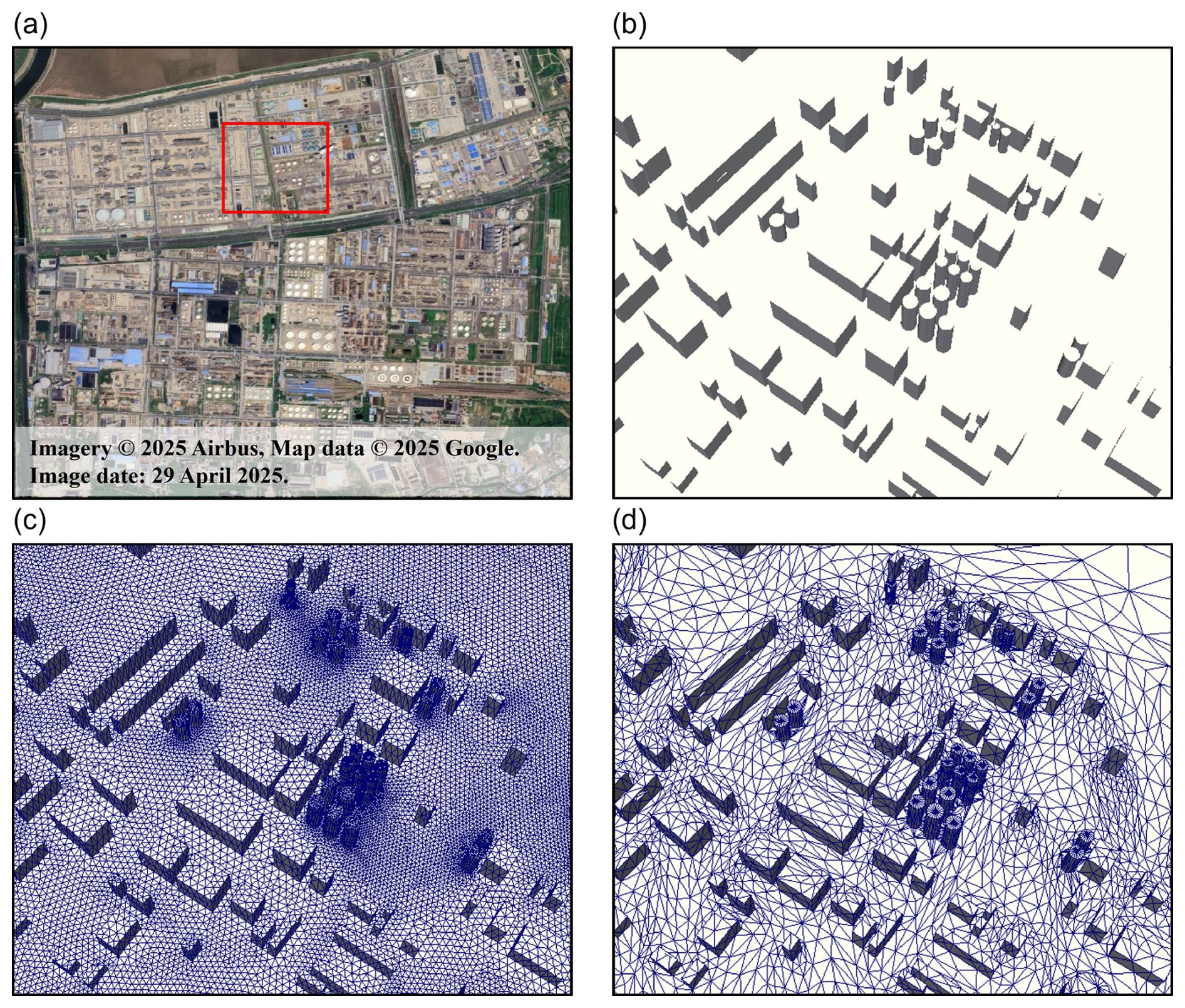
Figure 1Workflow of 3D urban geometry reconstruction and adaptive mesh generation: (a) high-resolution satellite imagery of the study area and a zoom-in view of (b) the reconstructed 3D urban geometry, (c) the initial unstructured mesh and (d) the adaptive mesh generated with DAMO during simulation. In (a), the satellite imagery is derived from Google Earth (https://earth.google.com/web/, last access: 10 February 2026). Imagery © 2025 Airbus, Map data © 2025 Google. Image date: 29 April 2025.
2.1.2 Urban turbulence inlet boundary conditions
Accurately prescribing inflow conditions is critical for reproducing the realistic aerodynamic behaviour of the atmospheric boundary layer as it interacts with the urban canopy. To achieve this, FluidUrban implements a turbulent inlet velocity profile driven by a synthetic eddy method (SEM). This approach superimposes realistic and transient turbulent fluctuations over a theoretical mean wind profile. The time-averaged streamwise velocity , is prescribed assuming a neutral atmospheric boundary layer (ABL) following the standard Log-Law profile or Power-Law Profile. To explicitly resolve the transient, energy-containing scales of turbulence entering the domain, the instantaneous velocity vector ui(x,t) at the inlet is computed as the sum of the mean flow and the instantaneous velocity fluctuations:
Following the SEM framework, the turbulent fluctuations, are generated by injecting a distinct number of synthetic eddies (N) and that convect through the inlet plane. The spatial and temporal distribution of these fluctuations is mathematically formulated as:
where aij represents the Cholesky decomposition of the prescribed local Reynolds stress tensor (Rij), which scales the intensity of the fluctuations. For each kth eddy, is a random sign distribution (typically) to ensure zero mean perturbation, fσ follows a normalized spatial shape function defining the coherent structure and characteristic length scale of the eddy, and xk(t) denotes the instantaneous position of the eddy center. The comprehensive mathematical derivation, including the specific geometric shape functions and the spatial-temporal numerical implementation of this SEM upon unstructured meshes within the Fluidity architecture, is detailed extensively by Pavlidis et al. (2010).
2.2 Model equations
The FluidUrban solves the 3D incompressible Navier–Stokes equations coupled with an advection–diffusion equation for scalar transport. To represent turbulence in the urban boundary layer, the model employs a large-eddy simulation (LES) framework. LES explicitly resolves energy-containing turbulent eddies while parameterising subgrid-scale (SGS) motions, thereby balancing numerical accuracy and computational cost. In this study, the SGS stress is parameterised using a second-order Smagorinsky model, with the Smagorinsky coefficient set to Cs=0.1 and a tensor-based filter length adopted for the anisotropic unstructured mesh. The velocity and pressure fields are discretised using a continuous Galerkin finite-element formulation, whereas the scalar transport equation is solved using a control-volume scheme. A theta method with θ=0.5 is used for time integration. Furthermore, the turbulent Schmidt number is set to Sct=0.7 to model turbulent diffusion of the scalar field. The filtered, incompressible Navier–Stokes equations under the Boussinesq approximation are employed for wind-field simulations:
where ρ is the fluid density, U the velocity vector, p the pressure, μ the dynamic viscosity, and g the gravitational acceleration.
For pollutant dispersion, the model employs the scalar advection-diffusion equation:
where c is the pollutant mass concentration, is the velocity vector, is the diffusion coefficient tensor, σ is the absorption coefficient (the term −σc is sometimes referred to as Rayleigh or linear damping), and F denotes source or reaction terms. In most environmental flow simulations, diffusion is assumed isotropic, so can be simplified as , with DAB denoting the binary molecular diffusion coefficient given by the Fuller et al. (1966) correlation:
In this equation, C is a constant fitting experimental data to ensure consistency between simulation results and measurements. T denotes the absolute temperature, p represents the ambient pressure, and b is the temperature-dependence exponent. In this study, b=1.75 is the temperature-dependent exponent, covering a wide range of binary gas systems. MA and MB denote the molecular weights of the two species, with the lighter species generally exhibiting higher diffusivity, and νi,A and νi,B are the molecular diffusion volumes of each gas component.
The pollutant mixture considered here comprises carbon dioxide (CO2, MA=44 g mol−1) and butane (C4H10, MB=58 g mol−1), with a mean density ρg≈1.8411 kg m−3 at standard conditions. The effective diffusion coefficient is obtained via a weighted average of the components, accurately reflecting mixture effects on transport (Nonaka, 2025).
2.3 WTE datasets
The performance of the FluidUrban v1.0 is evaluated using the WOTAN WTE dataset provided by the Environmental Wind Tunnel Laboratory (EWTL) at the University of Hamburg, Germany (Michel, 2023). This wind tunnel features a large test section with dimensions of 18 m in length, 4 m in width and 3 m in height. An idealised industrial-area model, geometrically scaled at 1:100 and representing a 300 m × 300 m real-world site, was employed to study flow and pollutant dispersion in a typical factory layout (Fig. 2). The model geometry was derived from aerial imagery and building data of an actual industrial park, ensuring a realistic representation of obstacle arrays and pollutant release scenarios.
The WOTAN WTE reproduced two atmospheric boundary-layer stability regimes, including medium roughness (MR) and high roughness (HR), corresponding to the surface characteristics of suburban open terrain and dense urban areas, respectively. These regimes are achieved by combining upstream turbulence generators with surface roughness elements. Following the VDI 3783/12 guidelines for physical modelling of the ABL (VDI, 2000), key flow parameters, including vertical wind speed profiles, turbulence intensity, turbulence energy spectra, and lateral uniformity, are measured and validated to ensure dynamical similarity between the wind-tunnel flow and the real atmosphere.
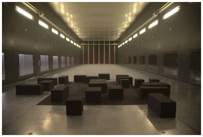
Figure 2Idealized industrial park model inside the WOTAN wind tunnel. View from the rear of the wind tunnel looking toward the model along the x-axis (from Michel, 2023).
2.4 Simulation configurations
2.4.1 Domain and boundary conditions
The validity of the comparison relies on the principles of physical similarity and Reynolds number independence, all simulations are performed at full scale, with the computational geometry replicating the wind-tunnel model. The computational domain precisely replicates the geometry of the wind-tunnel model (Fig. 3), representing an idealised medium density urban block. The layout comprises twenty rectangular buildings with varying shapes, each 15 m in height. The central building, measuring 60 m in length, 30 m in width and 15 m in height, contains two pollutant release openings (S1 and S2) on opposing side walls, each with an area of 16 m2.
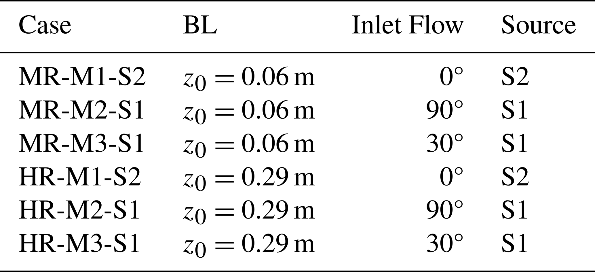
Following the COST Action 732 best-practice guidelines for computational wind engineering (Franke et al., 2011), the numerical domain is extended in the horizontal and vertical directions to minimize boundary influence on the internal flow field, yielding total dimensions of 1200 m × 1200 m × 150 m. A neutral ABL flow is prescribed via the boundary conditions. At the inlet, a power-law wind profile is applied to match the wind tunnel conditions for MR (z0=0.06 m, β=0.17) and HR (z0=0.29 m, β=0.23), as illustrated in Fig. 4. The outlet is set as a pressure boundary, permitting free development of the flow. Lateral and upper boundaries are specified as symmetrical planes with slip conditions, imposing zero normal velocity, while all ground and building surfaces are treated as no-slip walls. Consistent with the wind-tunnel campaign, three wind directions are simulated: a 0° inflow case (M1), a 90° case (M2), and a 30° tilted case (M3). For pollutant dispersion simulations, the main building acts as the emission source, with the two openings (S1 and S2) releasing pollutants at a constant rate (Fig. 3). The complete set of simulation configurations is summarised in Table 1.
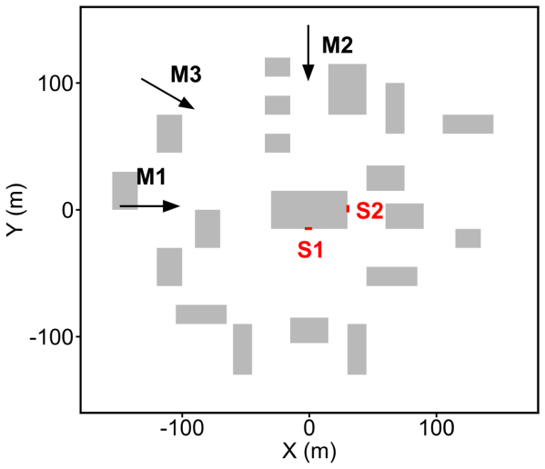
Figure 3Plan view of the idealized industrial park layout. Gray areas indicate buildings, S1 and S2 mark the two emission sources on the central building. Arrows indicate the three different inlet wind directions (M1: 0°, M2: 90°, M3: 30°).
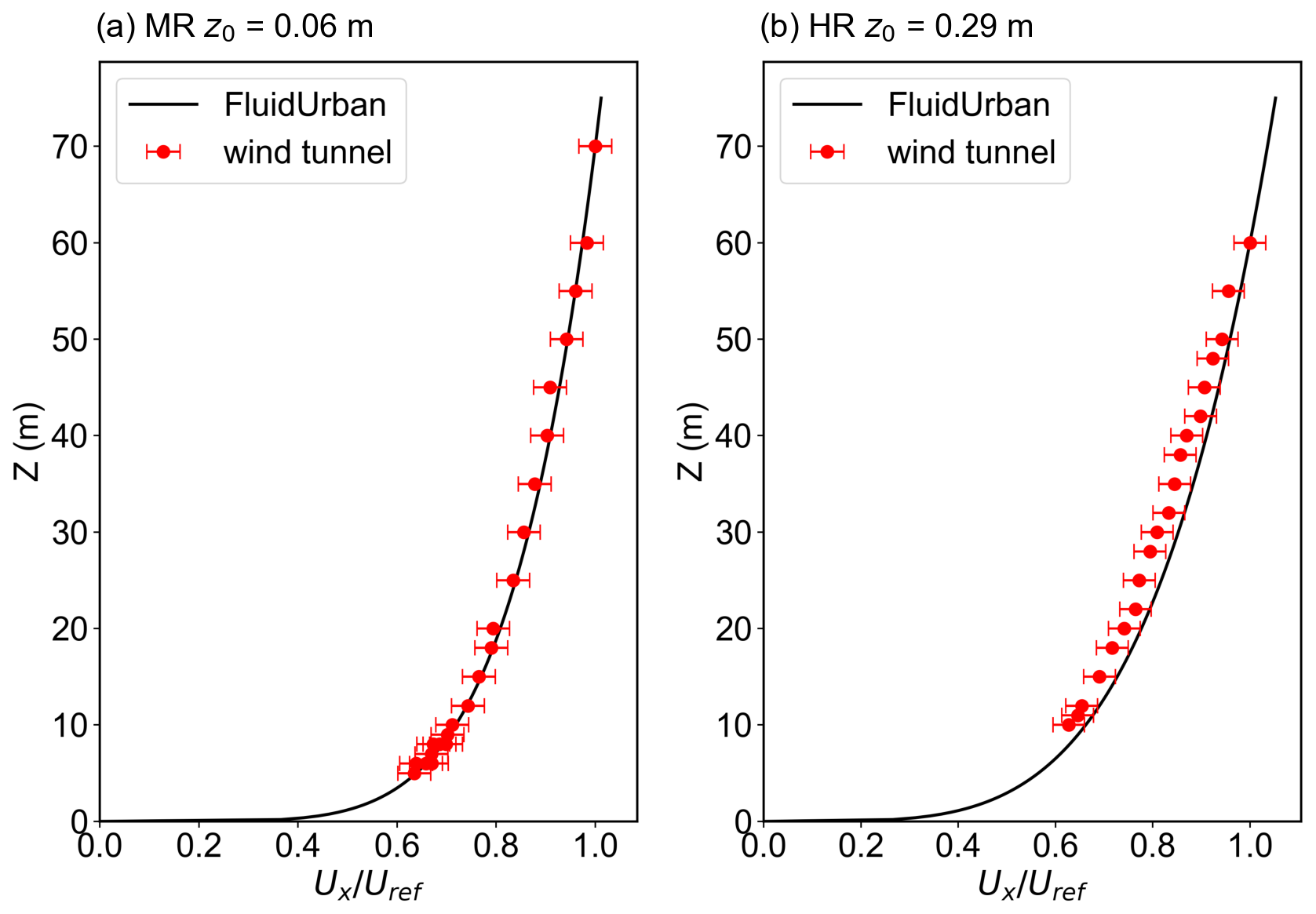
Figure 4Mean profiles of the inlet flow for the wind-tunnel experiment (red symbols) and the FluidUrban simulation (black solid lines), error bars indicate the standard deviation. (a) the medium roughness boundary condition (z0=0.06 m) and (b) the high roughness boundary condition (z0=0.29 m).
Table 1Key parameter settings for numerical simulation cases of the idealized industrial park. Case denotes the experimental case identification name. BL represents the boundary condition, expressed by the roughness height (z0). Inlet Flow indicates the wind direction of the inlet boundary, and Source refers to the emission source identification number used in the simulation.
Besides the mean profiles of the inlet flow, the inlet turbulence conditions were defined using the SEM for both the MR and HR cases. The inlet turbulence conditions are checked using the streamwise and lateral turbulence intensities, Iu and Iv. These quantities are defined as:
As shown in Fig. 5, the simulated profiles of both streamwise turbulence intensity Iu and vertical turbulence intensity Iv reproduce the main vertical trend observed in the wind-tunnel data, that is, relatively larger turbulence intensity near the ground and a gradual decrease with increasing height. Although some local discrepancies remain, the overall agreement indicates that the SEM-based inlet boundary conditions can reasonably represent the inflow turbulence characteristics required for the present simulations.
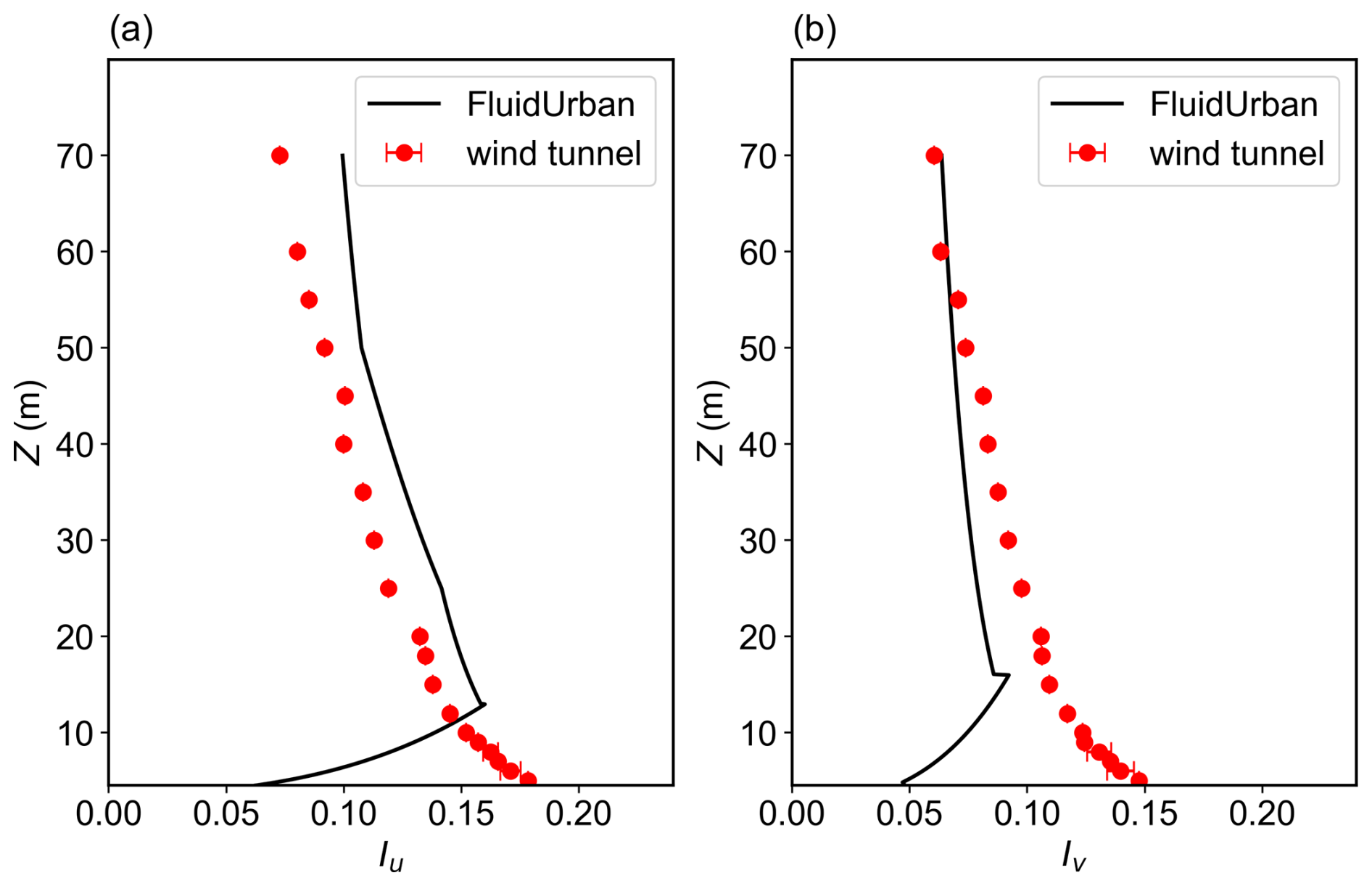
Figure 5Comparison of the vertical inlet turbulence intensity profiles between the FluidUrban synthetic eddy method (SEM) inlet boundary conditions (black solid lines) and the wind-tunnel experiments (WTE, red solid circles with error bars). Panel (a) presents the streamwise turbulence intensity (Iu), and panel (b) presents the lateral turbulence intensity (Iv).
2.4.2 Mesh adaptivity setting
A notable feature of the FluidUrban model is its advanced anisotropic dynamic mesh adaptivity functionality, which enables efficient capture of multi-scale physical processes through continuous optimisation of mesh distribution (Zheng et al., 2015, 2021; Wu et al., 2023). The core of this technique is an anisotropic mesh adaptivity method based on the Hessian matrix (Pain et al., 2001; Power et al., 2006), which aims to dynamically allocate computational resources to regions where they are most needed, while adhering to user-defined metric-control parameters. FluidUrban employs a fully a posteriori, metric-driven remeshing strategy. At each adaptation interval, the solver first advances the flow solution on the current mesh and then computes the Hessian matrix of the target fields. For the wind field and pollutant dispersion simulations in this study, the adaptive workflow proceeds as follows:
-
Target fields selection and Hessian matrix computation. The three velocity components u, v, and w are selected as primary target fields for adaptivity. For the pollutant-dispersion simulations, the concentration c is added as a fourth target field. At each adaptation step, the solver computes the Hessian of each field on the current mesh to quantify spatial curvature. For each target field f, the Hessian matrix is defined as:
Regions of strong curvature, such as shear layers and concentration fronts, are assigned finer resolution and more mesh elements.
-
Metric tensor construction. Following the Hessian-based metric construction of Pain et al. (2001), the metric tensor for field f is constructed as
where , with RH and containing the eigenvectors and eigenvalues of the Hessian. ϵf is a user-defined metric-control parameter, and γ is an O(1) scalar. In Pain et al. (2001), γ=1 is used. In the present implementation, γ=1 is also used, so Eq. (9) reduces to
The parameter ϵf controls the relative refinement weight: decreasing ϵf increases the weight of field f and therefore refines the mesh in regions where that field has strong curvature. Considering the physical characteristics of urban wind fields, a relatively large metric-control parameter is assigned to the streamwise wind speed u (ϵu=0.5 m s−1), whereas smaller values are applied to the vertical and lateral components .15 m s−1). This choice increases the refinement weight of lateral and vertical velocity variations in regions affected by building-induced flow separation, recirculation and vertical motions. For the air pollutant, the concentration metric-control parameter is set to ϵc=5 kg m−3. The parameter ϵf is a metric-control parameter, not a rigorous bound on the numerical error. With γ=1, the effective scaling is an ad-hoc scaling coefficient that controls the mesh size.
-
Metric intersection. When more than one target field is used, the individual metric tensors are combined using the metric-intersection operator ∩ following Pain et al. (2001). For two symmetric positive-definite metric tensors, M1 and M2, the intersection is the metric of the largest ellipsoid contained in both, so it retains the finer resolution requirement in each direction. To construct it, one metric, M1, is mapped to the unit sphere, and the other metric, M2, is transformed by the same mapping. With and , where Λ1 and Λ2 are the diagonal matrices of eigenvalues of the two metrics, M2 is transformed as:
where Q is the matrix of eigenvectors and is the diagonal matrix of eigenvalues of . In each principal direction, the unit sphere and the transformed second metric have semi-axes 1 and , respectively. The largest ellipsoid contained in both therefore takes the smaller semi-axis, which corresponds to
The corresponding metric is
and transforming back to the original space gives the final metric
For more than two target fields, the operation is applied pairwise. The operation is associative, each pairwise merge returns the largest ellipsoid contained in both inputs,so the pairwise grouping does not affect the result. The composite metric can therefore be written as
where Mu, Mv, Mw, and Mc are the metric tensors associated with the velocity components u, v, and w and the concentration c. Mc is included only in the pollutant-dispersion simulations. In the present implementation, the merges are performed successively, starting from the first target field, i.e. . The resulting composite metric preserves the refinement requirements of all target fields.
-
Metric smoothing and node-count limit. The composite metric tensor is smoothed to suppress abrupt local variations in the cell size that could lead to numerical instability. The maximum number of nodes is a safety cap in Fluidity: if the adaptivity algorithm attempts to exceed the prescribed maximum, the desired mesh is coarsened globally until it fits within the limit. To fully exploit the adaptive mesh, the maximum number of nodes is usually set to a relatively large value, so that the cap is rarely reached and the mesh size is controlled by ϵf and the Hessian. In this study, the maximum number of nodes is set to 2.0×10⁵. After adaptation, the node count is approximately 1.4×10⁵–1.9×10⁵ nodes (Table 5), within the 2.0×10⁵ node cap. The initial mesh at t=0 is generated before the first adaptivity step and is not subject to this cap. The cap is therefore not active, and the mesh size is controlled by ϵf and the Hessian.
-
Mesh generation and solution transfer. The optimised metric tensor is passed to the mesh generator, which employs the h-adaptation method (Pain et al., 2005) to produce a new anisotropic unstructured mesh. Field variables from the original mesh are interpolated onto the new mesh via a Galerkin projection algorithm (Farrell et al., 2009; Savre et al., 2016), completing one adaptive iteration.
In the evaluation simulations, the time step is set to 1 s, and DAMO is performed every 20 timesteps using the metric constructed from the selected target fields. The initial mesh resolution is 5 m in building-surface regions and 20 m elsewhere. As the simulation progresses, regions with strong gradients are refined to 2 m, while regions with weak gradients remain at or are coarsened to 20 m.
For comparison, a control case was established using a non-uniform fixed mesh (FIXM) generated via GMSH. To capture near-wall gradients while maintaining computational efficiency, the mesh resolution is refined to 2 m around the building surfaces and is configured to expand to 20 m at the top of the domain. This mesh configuration remains constant throughout the simulation. To isolate the impact of the mesh adaptivity, all physical parameterizations and boundary conditions in the control case (FIXM) are kept identical to those employed in the adaptive configuration. Consequently, the discretization strategy remains the sole varying factor between the two simulations, ensuring that simulated differences in the flow field and air pollutant are attributable exclusively to the mesh resolution and the dynamic refinement process. In this study, mesh resolution is defined in terms of the equivalent resolution, computed as a shape-weighted average across the domain (Müller et al., 2013). Specifically, the area of each triangular element is converted to the side length of an equilateral triangle of equal area, taken as its equivalent edge length. The global equivalent resolution is then obtained by an area-weighted average of these lengths, providing a consistent basis for comparing simulation errors and computational efficiency between DAMO and FIXM.
The FluidUrban simulations require a spin-up period to reach a statistically steady state. Because the six experiments do not reach this state simultaneously, a consistent comparison is ensured by analysing the final 1400 s of data (t=600 s to t=2000 s), using the experiment with the latest onset of steady state as the reference point.
2.5 Evolution metrics
The quantitative evaluation of the urban wind field simulation is first based on the Mean Error (ME) of the horizontal resultant wind speed is calculated as:
On this basis, the Mean Absolute Error (MAE) is further used to spatially average over all measurement points in order to evaluate the overall performance of the simulated wind speed field:
where and are the model simulated and observed resultant wind speeds at the ith observational sensor point, and N is the total number of observational sensors. The resultant wind speed is obtained from the horizontal velocity components as . To facilitate comparison among different experimental conditions, the wind speeds are normalized by the reference wind speed. Therefore, and are both dimensionless quantities. Smaller error values indicate better model performance.
For the quantitative evaluation of pollutant concentration simulations, three core statistical metrics are employed: fractional bias (FB), normalized mean square error (NMSE), and geometric mean bias (MG). They are defined as:
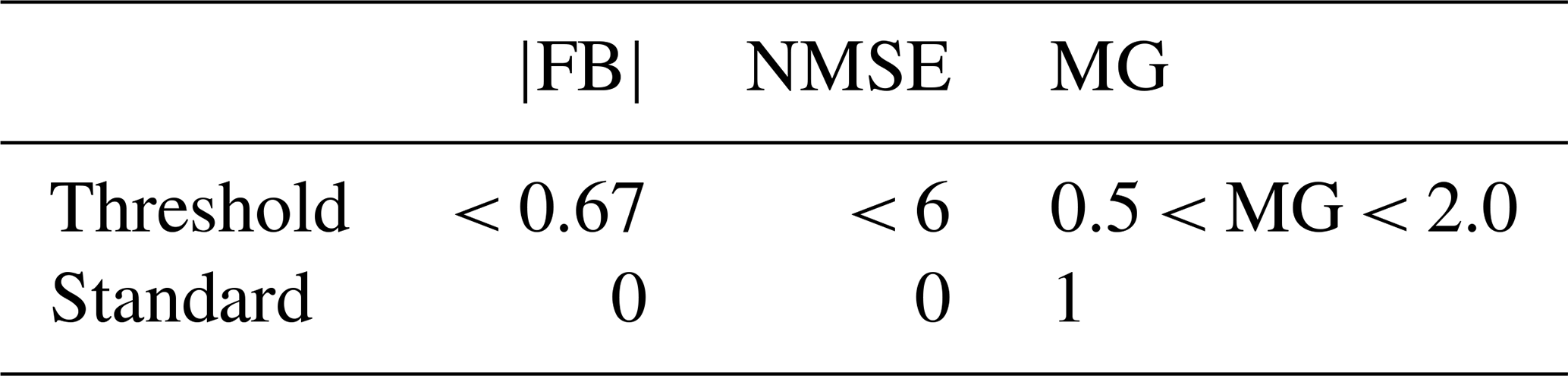
where and denote the arithmetic mean of observed and simulated values, respectively. FB measures systematic bias, NMSE reflects the random scatter between simulations and observations, and MG assesses the agreement in order of magnitude. According to established atmospheric model evaluation standards (COST Action ES1006, 2015), the ideal values for these metrics are |FB, NMSE =0, and MG =1. A high-performance model should produce results as close as possible to these ideal values. However, given that perfect agreement is unattainable under all conditions, this study adopts an additional set of threshold criteria from the literature (COST Action ES1006, 2015; Kurppa et al., 2020; Schalau et al., 2023; Gkirmpas et al., 2024), which are summarised in Table 2.
Table 2Threshold and standard reference values of Fractional Bias (FB), Normalized Mean Square Error (NMSE) and Geometric Mean bias (MG) used in model evaluation.
The evaluation of FluidUrban's simulation performance begins with an analysis of how the meshes evolves in response to complex wind flow dynamics. Benchmark comparisons are performed against the WOTAN WTE datasets to assess whether the DAMO accurately identifies and resolves the physical structures of interest. We first characterize the divergence between the FIXM and DAMO configurations. Taking the HR experiments as an example (Fig. 6), the fundamental divergence between these two types of meshes lies in the logic of computational resource allocation. The FIXM (Fig. 6a–c) employs an a priori static refinement. In such configuration, the resolution is predetermined and remains invariant, regardless of the transient nature of the flow or the development of turbulence. In contrast, the DAMO mesh (Fig. 6d–f) uses an a posteriori refinement mechanism, which automatically detects high gradient regions of the flow field, such as wake zones behind buildings, separated shear layers, and vortex cores, and allocates computational cells dynamically and locally to these key regions.
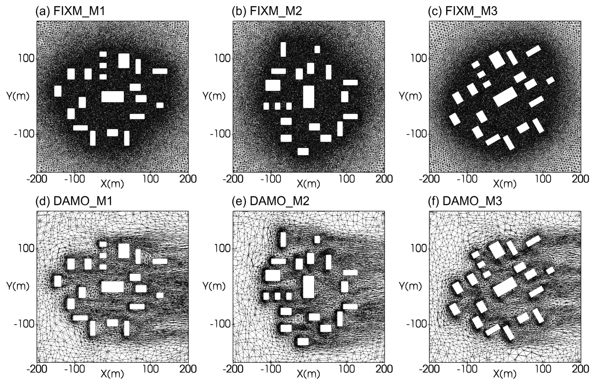
Figure 6The horizontal distributions of meshes at 2 m height for FIXM (upper row) and DAMO (lower row) simulations with inflow angles of 0° (left column), 90° (middle column) and 30° (right column) for M1, M2 and M3, respectively.
To further check the 3D mesh adaptivity on the vertical distribution of the mesh, the vertical cross-sections are presented in Fig. 7, which provide a clear diagnostic of how the 3D DAMO framework dynamically responds to the evolving flow field in vertical direction. While the FIXM (Fig. 7a–c) maintains a rigid, static resolution that ignores the development of the wake, the DAMO (Fig. 7d–f) exhibits a sophisticated a posteriori evolution. As the flow interacts with the building clusters, the refinement algorithm autonomously identifies the formation of separated shear layers and their subsequent downstream propagation. This is particularly evident in the extended wake regions, where DAMO maintains a high-density mesh to resolve the turbulent kinetic energy and velocity deficits that characterize the downstream flow. This ability to track the flow evolution ensures that the complex building-atmosphere interactions, which are often lost in static, coarse-grid regions, are captured with high numerical fidelity. Consequently, the DAMO configuration provides a more physically consistent representation of the downstream transport of momentum and scalars compared to the fixed-mesh baseline.
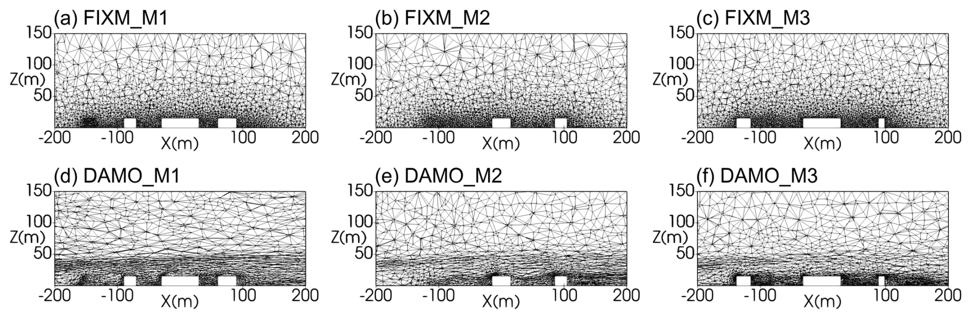
Figure 7The z-x cross-section of meshes at y=0 m for FIXM (upper row) and DAMO (lower row) simulations with inflow angles of 0° (left column), 90° (middle column) and 30° (right column) for M1, M2 and M3, respectively.
To quantitatively detail the spatial resolution characteristics of the simulations, Fig. 8 presents the mesh-size distribution statistics for both the fixed (FIXM) and dynamically adaptive (DAMO) meshes under the medium and high roughness conditions. In this analysis, the local mesh size is evaluated based on the unique edge lengths of the unstructured elements. The length of each edge is calculated using the Euclidean distance formula:
For edges shared by adjacent cells, we ensure that each edge is counted only once by sorting the endpoints and removing duplicates. The FIXM distributions are dominated by a sharp peak at 2 m, reflecting the prescribed near-building refinement, and decay rapidly beyond about 5 m. In contrast, the DAMO distributions are broader. They retain a 2 m component in the near-building region but exhibit a pronounced peak near 10 m and a tail extending to approximately 30–40 m, reflecting dynamic coarsening of weak-gradient regions while fine resolution is retained where the flow and scalar gradients are strong. This qualitative pattern is consistent across all six cases, indicating that the adaptivity responds robustly to changes in surface roughness and inflow direction. The total cell counts range from 751 251 to 824 572 for FIXM and from 1 016 526 to 1 025 882 for DAMO. These counts further show that DAMO does not simply refine the mesh uniformly, but redistributes cells from weak-gradient to dynamically important regions.
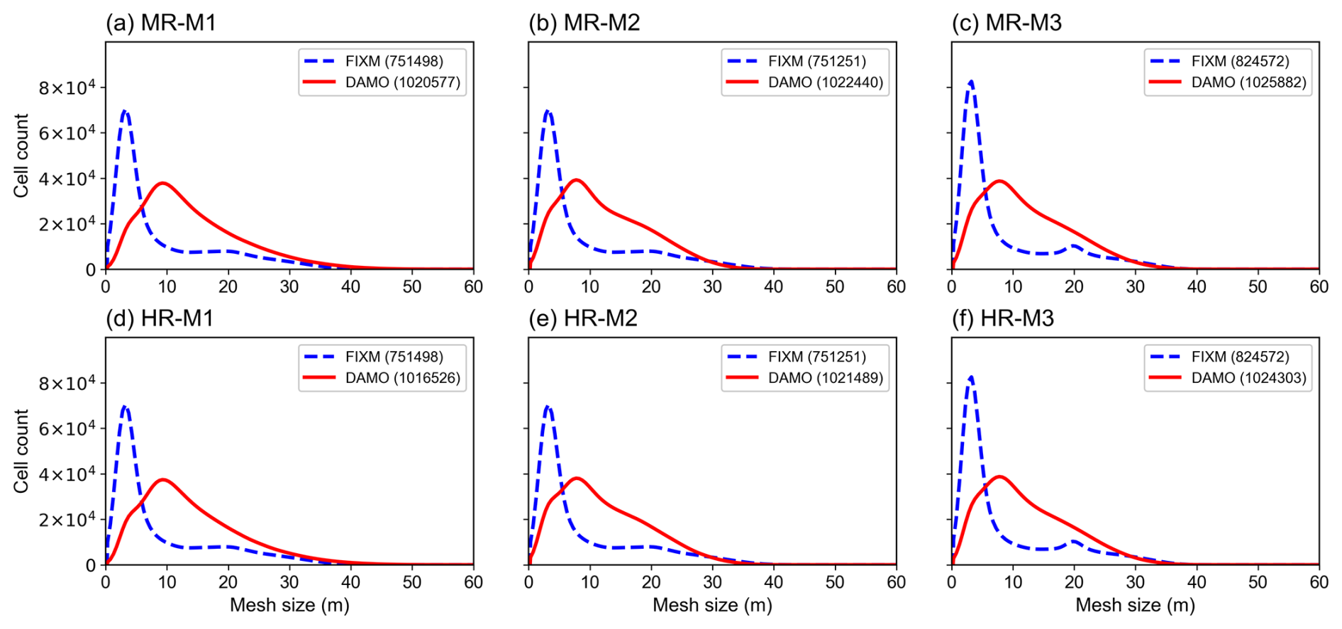
Figure 8Mesh size distributions for the FIXM (blue dashed lines) and DAMO (red solid lines) simulations under medium roughness (upper row) and high roughness (lower row) conditions. The three columns correspond to inflow directions M1 (0°), M2 (90°) and M3 (30°). The horizontal axis is the local mesh size and the vertical axis is the number of cells in each size bin. Values in parentheses give the total number of mesh cells for each case; DAMO results are shown at t=2000 s.
3.1 Wind Speed
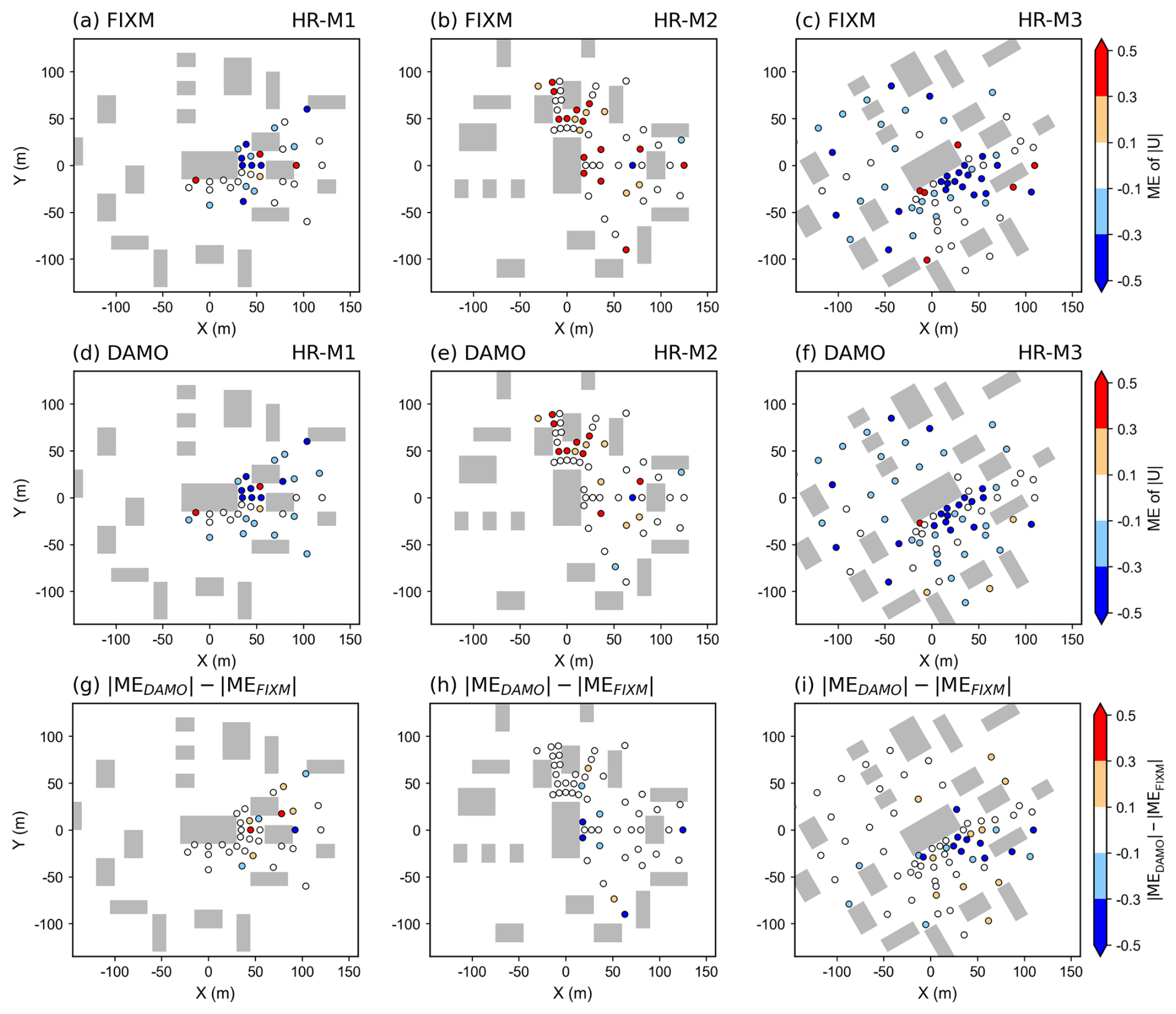
To evaluate the improvement in performance achieved by the DAMO in urban wind speed simulation, the spatial distributions of ME for horizontal wind speed () at 2 m height are presented. These are shown for both MR and HR conditions in Figs. 9 and 10, respectively. In MR condition (Fig. 9), the DAMO simulations generally exhibit lower MAE values across most regions. Particularly, in the MR-M2 case, the ME values of DAMO simulations in the vicinity of buildings are mostly confined within ±0.1, whereas the FIXM simulations show significantly higher deviations in the same areas. And also, in the oblique inflow case MR-M3, the adaptive meshes refine dynamically along the shear and wake directions (Figs. 6f, 7f), tracking the critical flow paths to maintain high accuracy (Fig. 9f). Additionally, the absolute difference of ME between the DAMO simulations and the FIXM simulations was computed (Fig. 9i), where more negative values indicate smaller errors in the DAMO results. However, in the MR-M1 case, the DAMO simulation exhibits limited improvement over the FIXM simulation. This is likely because the primary inlet flow direction of 0° aligns parallel to the street canyon, generating a stable canyon flow with weak gradient that diminishes the need for adaptive refinement. The errors at all observation points were further averaged to calculate the MAE, which was then used to quantitatively assess the performance of DAMO in urban wind speed simulations. Consistent with the spatial distribution results, the DAMO simulations in the MR-M2 and MR-M3 cases show a significant reduction in MAE. In the MR-M1 case, however, the MAE increases slightly, while the difference remains within approximately 0.03.
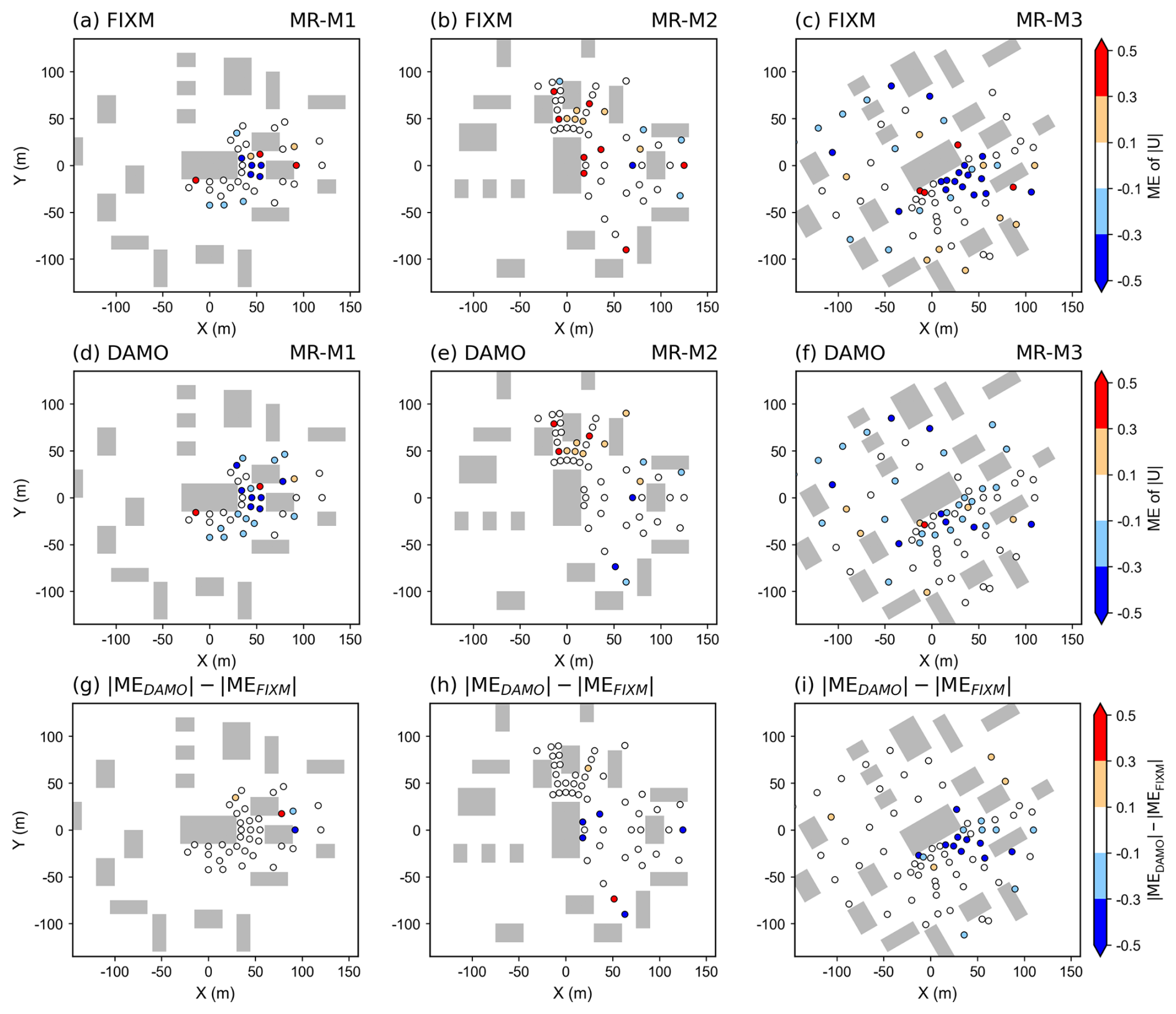
Figure 9Spatial distribution of the Mean Error (ME) for 2 m horizontal wind speed under the medium roughness (MR) condition from FIXM (upper row) and DAMO (middle row) simulations, and the difference between the two simulations (lower row), with inlet flow direction of 0° (left column), 90° (middle column) and 30° (right column). The circle marks indicate the locations of the observational sensors in WOTAN wind tunnel experiments.
Table 3Spatially averaged Mean Absolute Error (MAE) of 2 m horizontal wind speed. In each case, the smaller error between the FIXM and DAMO simulations is shown in bold.
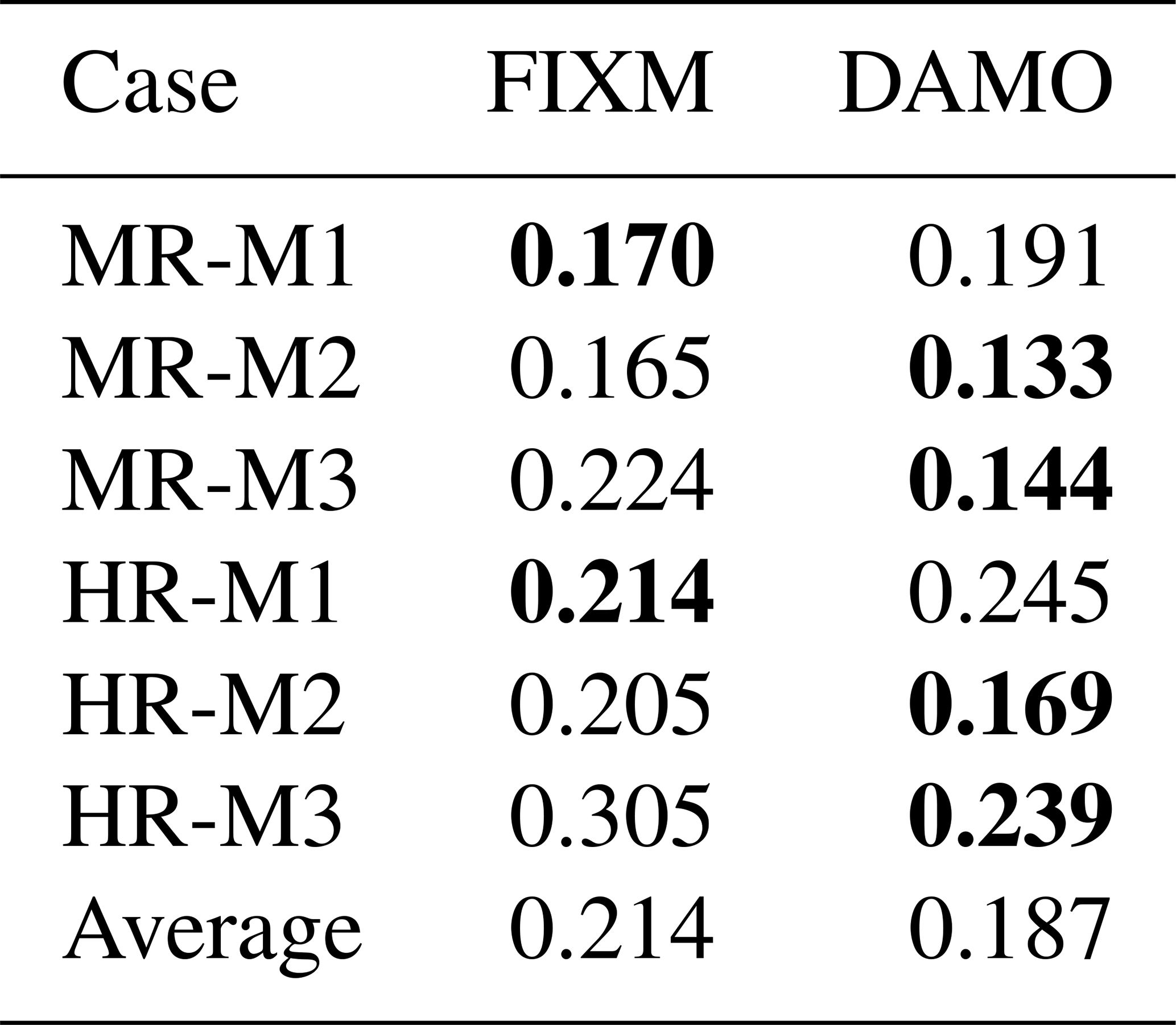
The transition from MR condition (Fig. 9) to HR condition (Fig. 10) results in a marked decline in the overall accuracy of both the FIXM and DAMO approaches. This decline is likely attributed to the intensified interaction between the incoming turbulence and the dense building canopy under high surface roughness conditions, which generates smaller and more energetic turbulent structures that impose higher demands on the mesh resolution. Despite such challenges, the DAMO maintains superior error control in critical regions such as building wakes, confirming its robustness in complex flows. Furthermore, as quantified in Table 3, the DAMO simulations under HR conditions achieve lower MAE for the inlet flow directions of 90° (HR-M2) and 30° (HR-M3), consistent with the MR conditions. In particular, in the HR-M3 case, the DAMO shows an error reduction of nearly 0.07. This consistent performance across various conditions further confirms the robustness of the DAMO method.
3.2 Wind Direction
Following the evaluation of wind speed, this subsection accesses the performance of DAMO in simulating wind direction. Figures 11 (MR) and 12 (HR) present a visual comparison between the near-surface (2 m) wind vector fields from the simulations and WTE datasets, illustrating the ability of two mesh types to resolve local flow patterns.
In the M1 and M2 cases (0 and 90°), the improvement of DAMO against FIXM is not particularly pronounced, probably due to the fact that, for inflow directions aligned with the main street axes, the near-surface airflow is primarily governed by relatively steady channelling effects and fixed velocity gradients. In contrast, in the M3 case (inflow angle of 30°), a more realistic and complex scenario, the DAMO results are much closer to the WTE measurements. DAMO automatically identifies and refines critical zones such as building windward corners and lateral separation regions, where strong pressure gradients and momentum fluxes determine the local wind deflection. A quantitative assessment based on MAE of wind direction further confirms the performance of DAMO. Similar to the spatial distribution, for the M3 case, DAMO reduces the MAE by 38.4 % and 36.1 % for MR and HR simulations, respectively (Fig. 13), underscoring its reliability in simulating realistic urban wind fields. Although the improvement is more modest for the M1 and M2 cases (0 and 90°), DAMO still achieves a reduction in wind direction MAE of up to 20.5 %.
The advantage of DAMO is more significant for wind direction simulation compared to wind speed simulation, as wind direction is largely governed by local velocity gradients and vorticity, which are precisely the flow structure targeted by the DAMO refinement criteria. Moreover, accurately resolving these fine vortex structures is crucial for realistic pollutant dispersion modelling, which will be explored in Sect. 3.4.
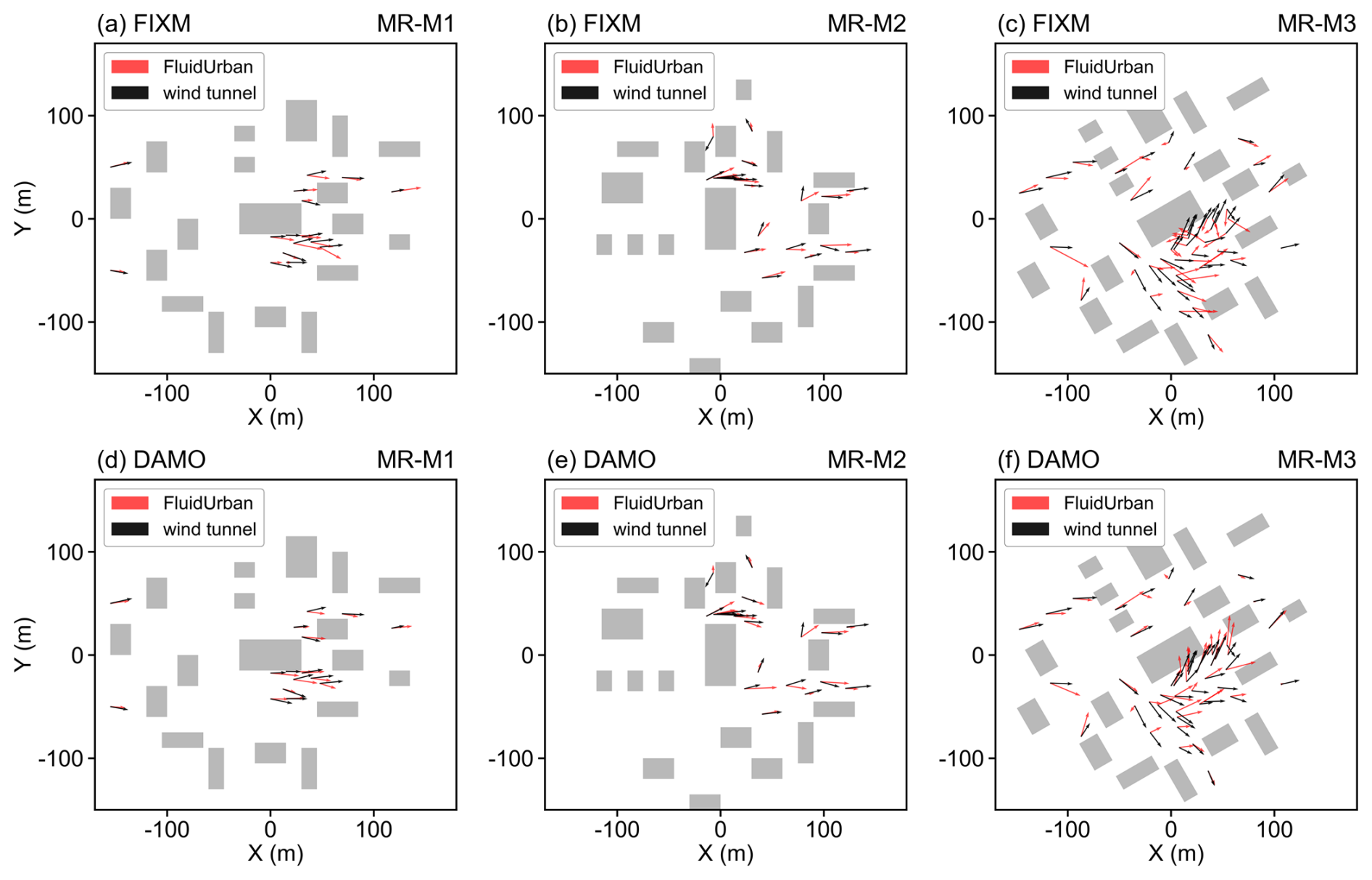
Figure 112 m horizontal wind vectors under the medium roughness (MR) condition of the simulation (red arrows) with wind-tunnel experiment (black arrows). Panels (a)–(c) present the FIXM simulation results, and (d)–(f) mean the DAMO simulation results, with inlet flow direction of 0° (left column), 90° (middle column) and 30° (right column).
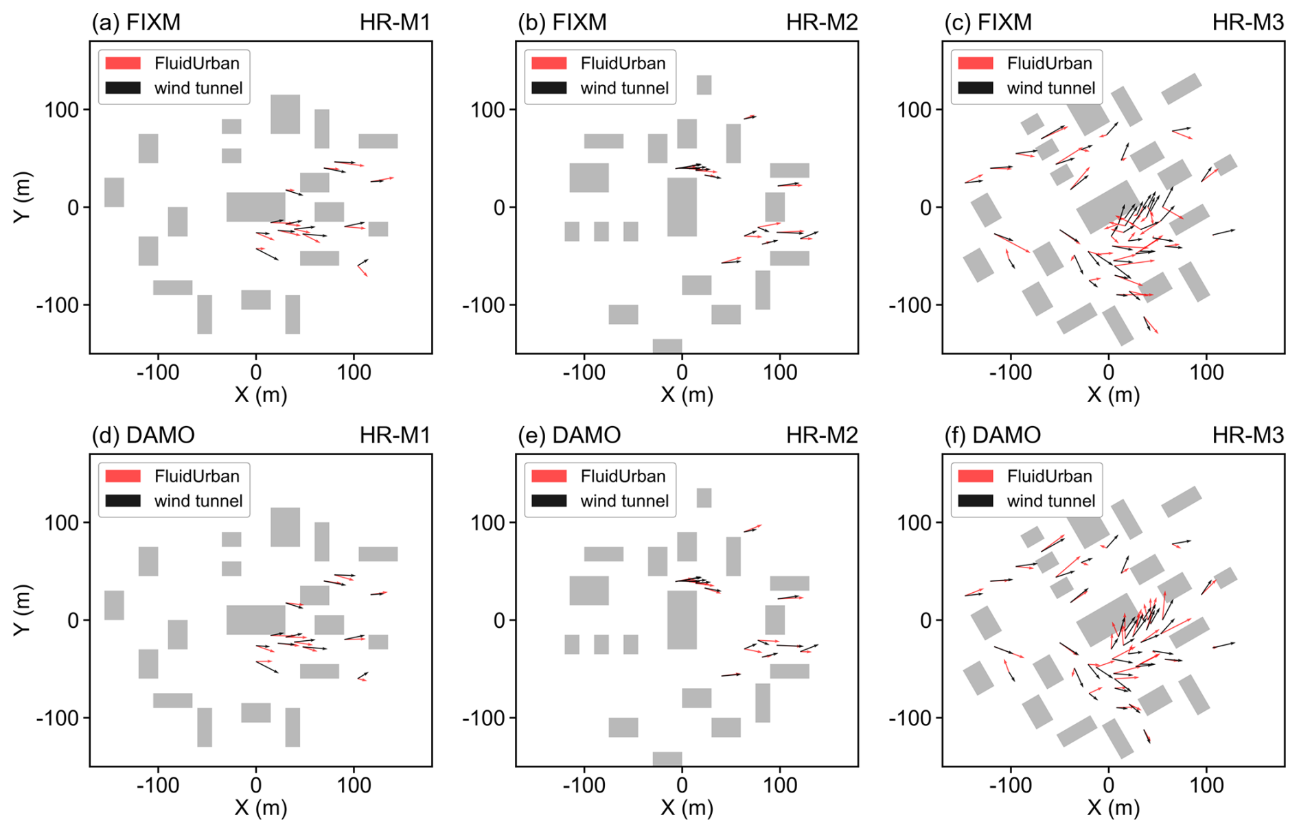
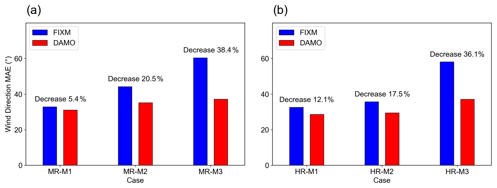
Figure 13The spatially averaged Mean Absolute Error (MAE) of 2 m horizontal wind direction under (a) Medium roughness condition (MR) and (b) High roughness condition (HR). The labels “Decrease” and the associated percentages represent the reduction in MAE achieved by DAMO relative to FIXM.
3.3 Turbulent Intensity
This section further evaluates FluidUrban's ability to predict velocity fluctuations through turbulent intensity profiles. Since turbulent intensity reflects the magnitude of velocity fluctuations relative to the mean flow, it provides a more stringent measure of the model's ability to represent the complex unsteady turbulent structures induced by building–flow interactions. In this section, the streamwise and lateral turbulent intensities, Iu and Iv, were calculated from the velocity time series at each measurement point using the same sampling interval as in the wind tunnel experiments, ensuring temporal consistency and comparability between simulations and measurements.
Figure 14 presents the vertical profiles of Iu and Iv under MR and HR conditions across all cases. Overall, both FIXM and DAMO underestimate turbulent intensity to varying degrees, but notable differences exist between the two approaches. FIXM shows a pronounced negative bias at nearly all heights and inflow conditions, particularly in the wake-dominated region and near the roughness sublayer, which is consistent with the stronger numerical dissipation associated with its static pre-refinement strategy. By contrast, DAMO reproduces both the magnitude and vertical variation of turbulent intensity more accurately by dynamically refining high-gradient regions such as separated shear layers, building wakes, and vortex cores, thereby better preserving velocity fluctuations. Across all FluidUrban cases, DAMO remains closer to the measured profiles, indicating greater adaptability in capturing complex turbulent structures.
The error distributions further confirm this conclusion (Fig. 15). The signed error is defined as the simulation result minus the wind tunnel result, so negative values indicate an underestimation of turbulent intensity. Although both configurations exhibit predominantly negative errors, indicating a systematic underestimation, the boxplot for DAMO lies closer to the zero-error baseline and shows a smaller spread, suggesting not only reduced bias but also improved stability in predicting turbulent fluctuations. Overall, DAMO significantly alleviates the smoothing effect observed in FIXM and better preserves the unsteady characteristics of the flow field.
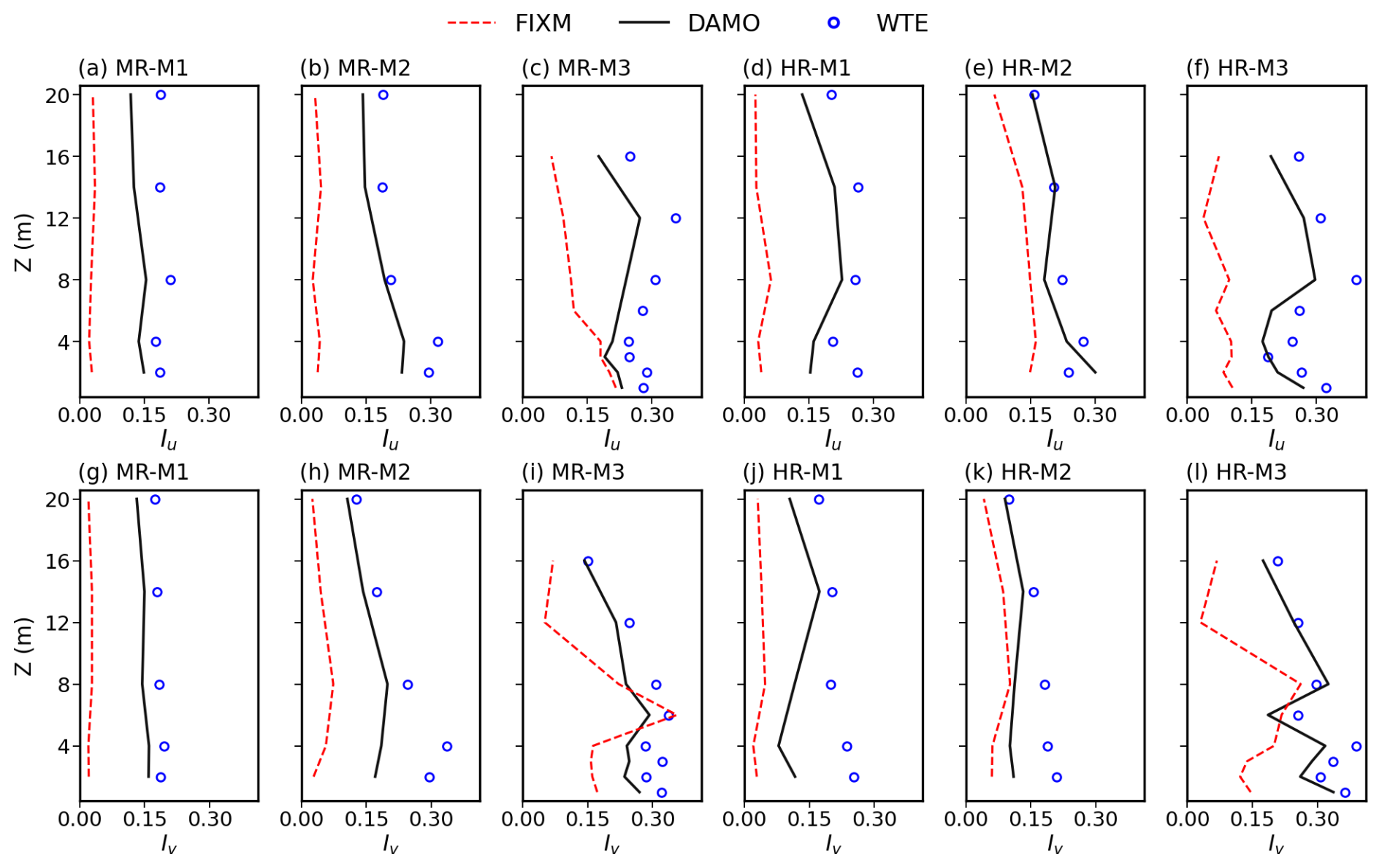
Figure 14Comparison of the vertical turbulence intensity profiles between the FluidUrban simulations and wind-tunnel experiments (WTE). The upper row (a–f) presents the streamwise turbulence intensity (Iu), and the lower row (g–l) presents the lateral turbulence intensity (Iv). Results are shown for the FIXM model (red dashed lines), the DAMO model (black solid lines), and the WTE observational data (blue open circles) across the medium (MR) and high (HR) roughness test cases.
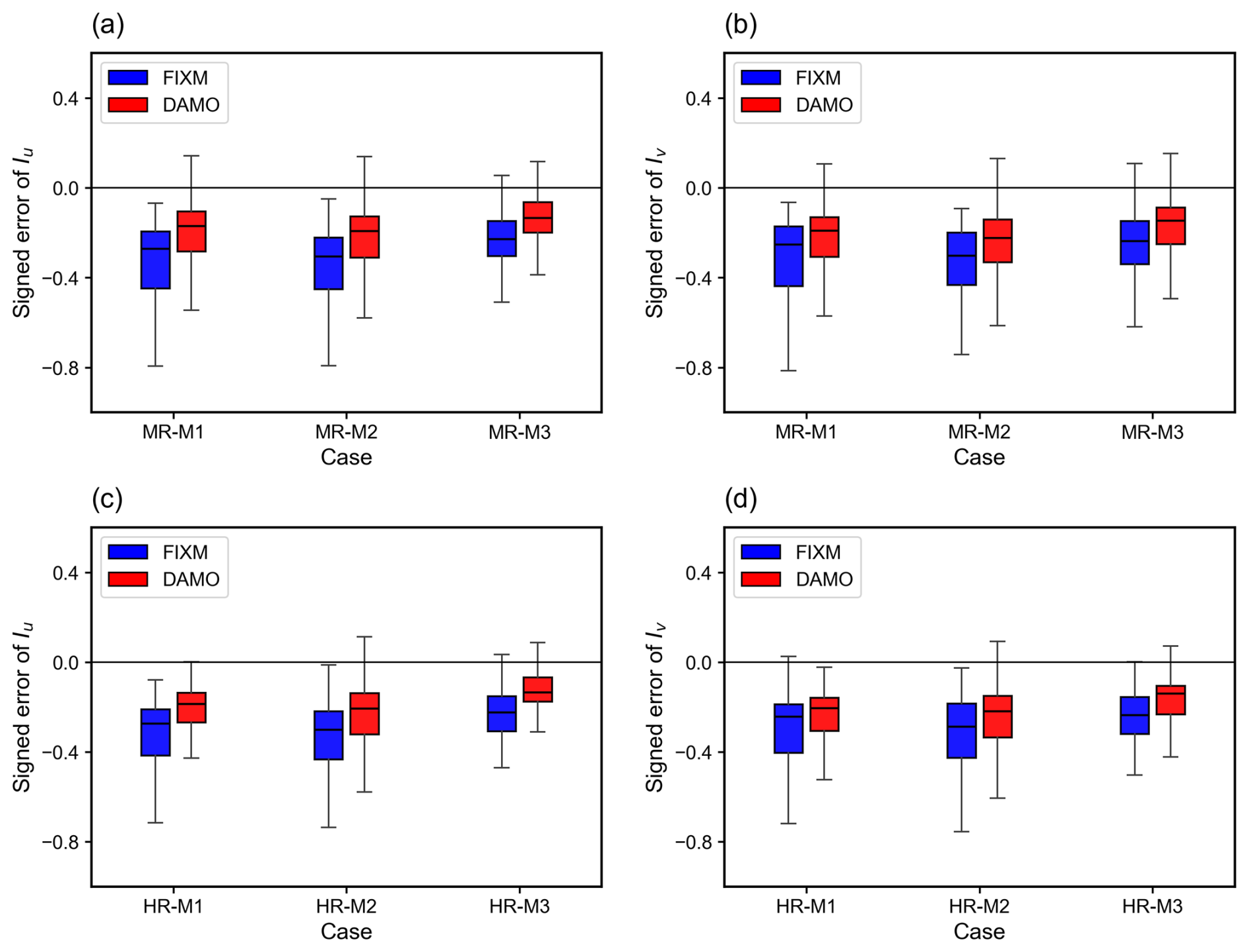
Figure 15Boxplots of the signed errors for the simulated streamwise (Iu) and lateral (Iv) turbulence intensities under medium roughness (MR, upper row) and high roughness (HR, lower row) conditions. For each boxplot, the box indicates the interquartile range, the horizontal line within the box represents the median, and the whiskers denote the overall data range. The solid horizontal black line marks the zero-error baseline.
3.4 Pollutant Dispersion
This section evaluates the improvement in pollutant dispersion performance achieved with DAMO. Spatial comparisons of plume distribution under MR and HR conditions are shown in Figs. 16 and 17. For inflow cases M1 and M2, the FIXM simulations exhibit pronounced numerical diffusion, resulting in smeared concentration gradients and excessive dilution. In contrast, DAMO effectively reduces this non-physical spreading and capture the sharp gradients of pollutant concentration, resulting in notable improvements in plume trajectory and concentration distribution (Figs. 16a, b, 17a, b). The relatively large discrepancy between the FIXM simulations and the measurements in Figs. 16c and 17c is a direct consequence of the inaccurate wind field prediction shown earlier in Figs. 11c and 12c. Pollutant transport is fundamentally driven by the underlying flow field. Because FIXM fails to accurately capture the correct flow topology, it inevitably fails to reproduce the correct plume deflection direction. Finally, it should be emphasized that DAMO does not theoretically guarantee better performance in every conceivable scenario. Rather, it is designed to provide significantly improved accuracy when the flow field is strongly heterogeneous, exhibits sharp transient gradients, and contains moving physical structures.
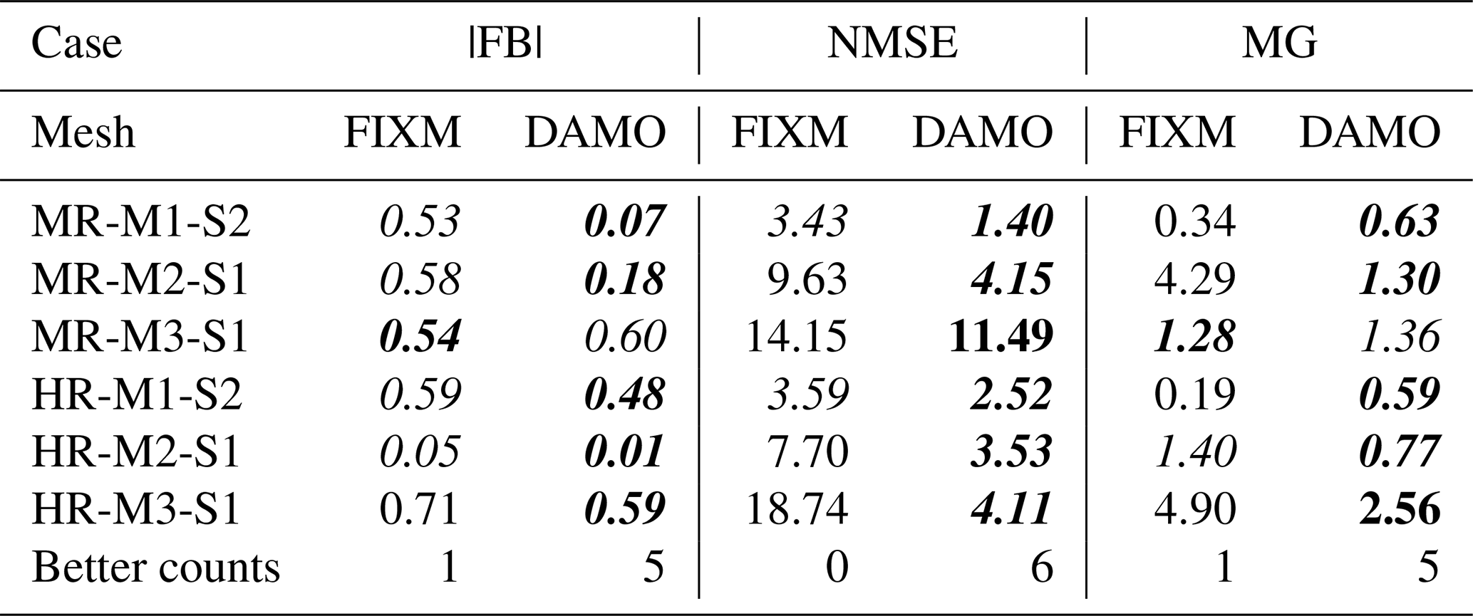
Further quantitative assessment employs three complementary statistical metrics: FB, NMSE, and MG (Table 4). DAMO meets the COST Action ES1006 acceptance criteria in 89 % of cases (16 of 18 metrics meeting thresholds), significantly exceeding the 50 % compliance rate of FIXM (9 of 18). The most pronounced contrast occurs for NMSE, a metric highly sensitive to extreme deviations, where DAMO outperforms FIXM in all six cases. This advantage arises from the framework's physical driven allocation of computational resources, which concentrates mesh refinement in dynamically critical regions, thereby reducing local errors and numerical scatter. The resulting improvement in predictive stability confirms the superior accuracy and reliability of DAMO for urban pollutant dispersion simulations.
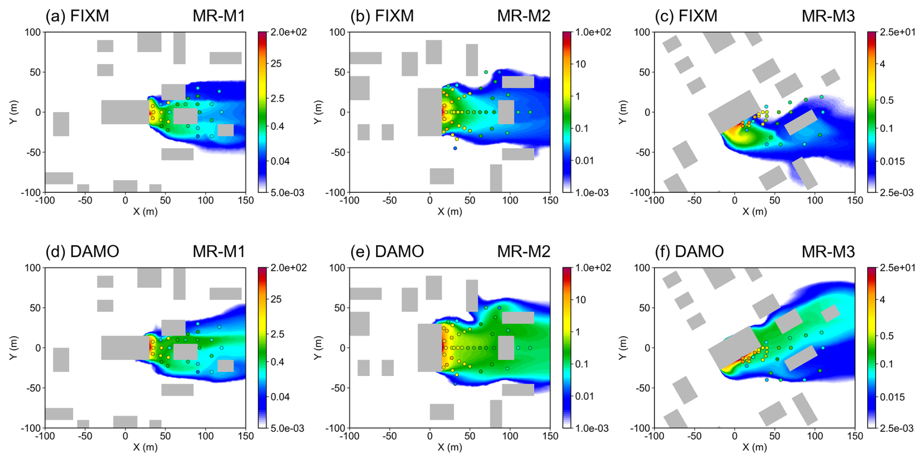
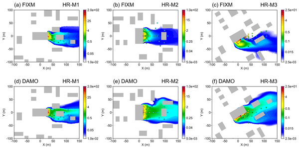
Figure 16Pollutant gas concentration slice at 2 m above ground under medium surface roughness (shaded, units: kg m−3). Gray boxes represent buildings, and the circles represent experimental measuring points. (a–c) the simulation results of FIXM, and (d–f) the simulation results of DAMO, same hereafter.
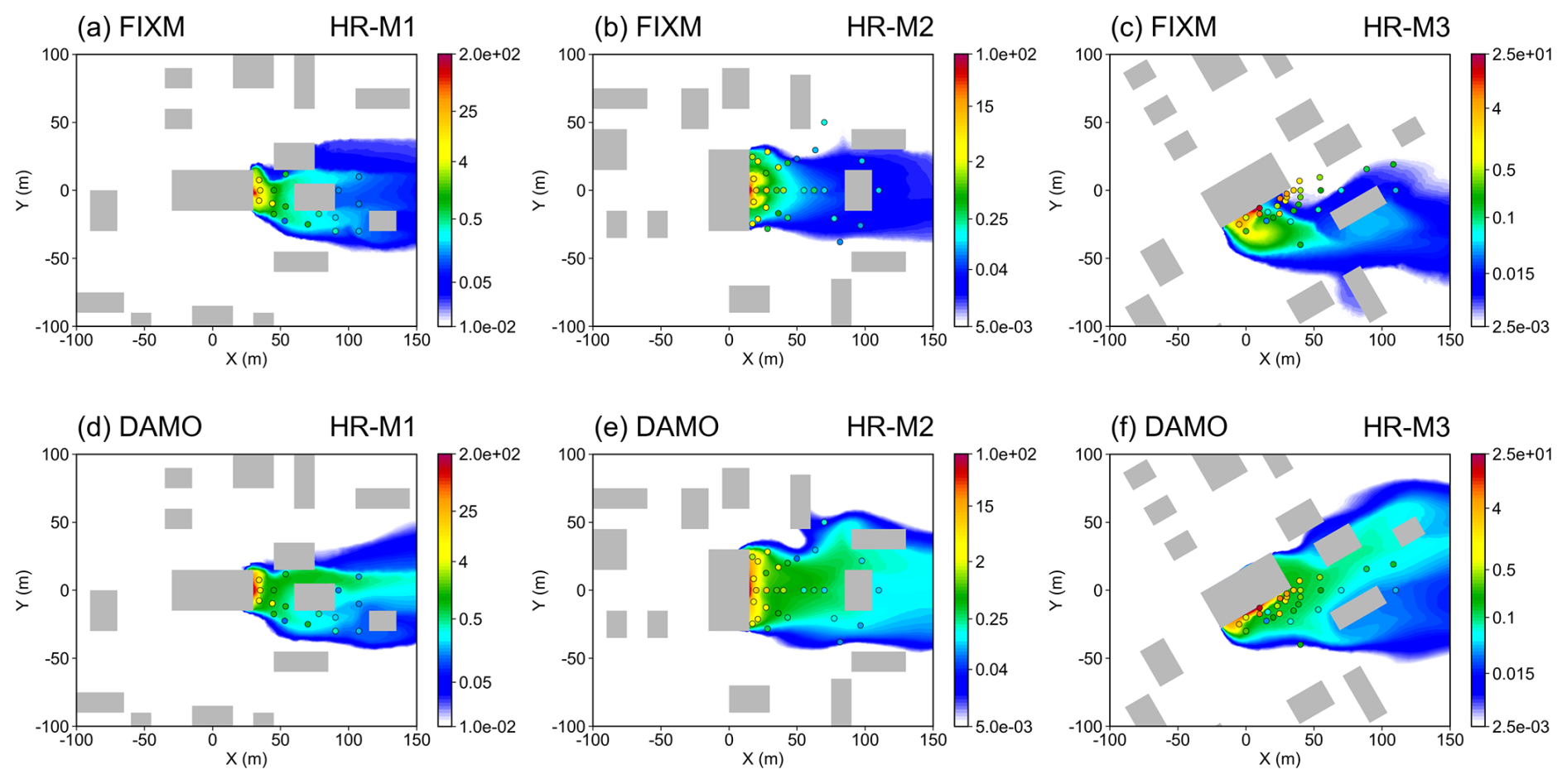
Table 4Quantitative performance indicators for pollutant gas dispersion for all investigated cases for FIXM and DAMO. Italic values denote threshold-compliant indicators, bold values indicate results closer to the standard, and “Better counts” is the number of indicators closer to the standard per case.
3.5 Computational Performance
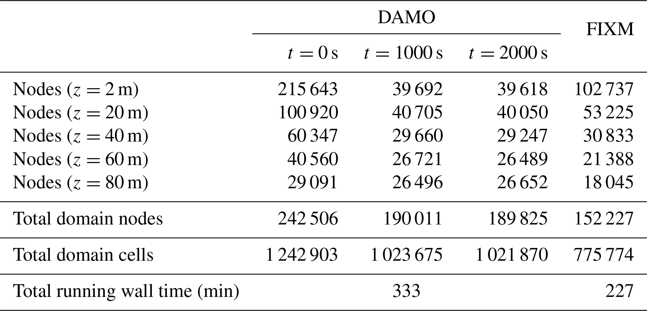
The comparison of computational efficiency in this study is based on the current FIXM and DAMO simulations, which already exhibit a high level of consistency in their overall morphological distributions. In the DAMO, the mesh resolution dynamically evolves with the flow field; accordingly, the number of mesh nodes was documented at three representative time stages: the initial stage (t=0 s), the intermediate stage (t=1000 s), and the final stage (t=2000 s). For the FIXM, the total number of nodes and cells remains constant throughout the entire simulation (Table 5). From the perspective of spatial resource allocation (Fig. 18), the computational nodes in DAMO are concentrated precisely within plume zones exhibiting strong concentration gradients in near-surface regions critical for pollutant dispersion (z=2 m and z=20 m), while dynamically adding mesh elements to better capture the fully developed flow structures in these regions in the upper-layer space above the buildings (z=40 m). Considering that the total model domain height (150 m) is much greater than the building height (15 m), such enhanced resolution of the upper-layer flow results in a slightly higher total number of nodes and cells for the DAMO during the late simulation period. Table 5 and Fig. 8 give the total mesh sizes: FIXM contains 152 227 nodes (775 774 cells), compared with 189 825 nodes (1 021 870 cells) for DAMO at t=2000 s. Although FIXM exhibits a pronounced 2 m peak, its total node and cell counts are both lower than those of DAMO. Because FIXM remains unchanged throughout the simulation, this peak primarily reflects the prescribed near-building refinement rather than a larger overall mesh or any dynamic, solution-driven refinement. In this study, FIXM is used as a deliberately well-resolved and conservative fixed-mesh benchmark. While this design may lead to locally higher-than-necessary resolution in some near-building regions, a coarser FIXM would likely increase numerical diffusion and near-building errors and could artificially exaggerate DAMO's apparent advantage. The comparison is therefore conservative rather than biased in favor of DAMO. The DAMO peak near 10 m reflects dynamic coarsening in weak-gradient regions while fine resolution is retained where the flow and scalar gradients are strong.
Although dynamic adaptivity offers significant advantages in accuracy, it also introduces extra computational cost for mesh adjustment. At present, the DAMO simulations employ 189 825 nodes and require 333 min to complete, whereas the FIXM uses 152 227 nodes and finishes in 227 min. When normalized to an equivalent number of mesh nodes, the DAMO exhibits an approximately 17.6 % longer total simulation time compared with the FIXM. This quantifiable overhead highlights the “deliberate computational investment” undertaken to achieve higher physical realism and resolve complex flow structures, while underscoring the continued need for algorithmic optimization to further improve computational efficiency without compromising accuracy. Future work may consider applying moderate mesh coarsening in the upper-layer regions, thereby allocating more computational resources to the near-ground critical areas to further enhance overall model performance.
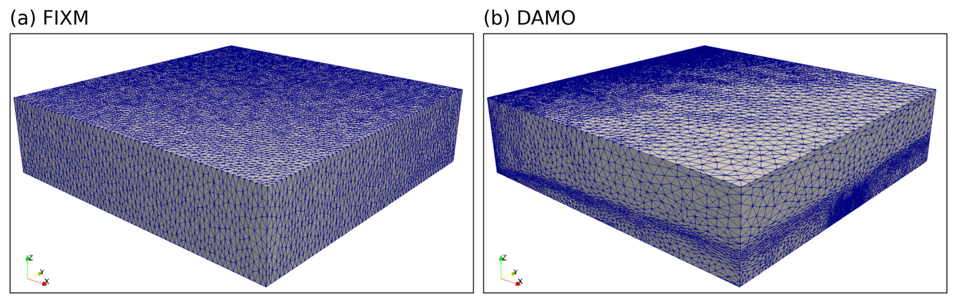
Figure 18Comparison of 3D model meshes generated by the FIXM (left) and DAMO (right) methods.
Table 5Comparison of mesh node and cell numbers and running times for the FIXM and DAMO configurations. Node counts are given at five height sections (z=2, 20, 40, 60, and 80 m); node and cell counts are given for the full computational domain. FIXM values are averaged over M1–M3, and DAMO values are averaged over the six experiments (MR and HR, M1–M3) at t=0, 1000, and 2000 s. Total running wall time refers to the full simulation, not to individual stages.
To further check its performance in a realistic application, FluidUrban was employed to simulate the wind field over the Industrial Park of Zhenhai Refining and Chemical Company (ZRCC) in Ningbo, Zhejiang Province, China. The 3D geometry of the Industrial Park was reconstructed using the approach described in Sect. 2.1.1, and the corresponding computational domain and mesh was subsequently simulated using the DAMO method (Fig. 1).
At the inlet, a northerly inflow was specified according to the climatological prevailing wind direction in winter around the Industrial Park. The mean streamwise inflow profile was defined as a function of the vertical coordinate z and followed the standard logarithmic law above the roughness height z0, as given in Eq. (22), while the remaining flow components were set to zero. At the outlet, a zero-stress condition was applied and the pressure was fixed at 0 to allow the flow to develop freely. No-slip boundary conditions were imposed on the ground and building surfaces. The lateral boundaries and the top boundary were treated as symmetry planes with slip conditions, thereby alleviating the need to resolve far-field flow details. The wind field was then simulated using the DAMO method. DAMO was employed with grid sizes ranging from 2 to 1000 m; with a dynamical updated frequency of every 10 time steps, and the time step was also dynamically adaptive under a CFL constraint of 5.
where u* is the friction velocity and κα=0.41 is the von Karman constant. In this study, , corresponding to a wind speed of approximately 2.4 m s−1 at z=10 m based on the climatological winter wind speed over the Industrial Park, and the roughness length was set to z0=0.84 m. After the flow reached a statistically steady state, the simulated wind field over the entire computational domain is presented in Fig. 19a. Under the complex morphology of the industrial park, the model resolves the pronounced spatial heterogeneity of the wind field caused by blocking and channeling effects. A close-up analysis of the flow field (Fig. 19b, zooming in on the region indicated in Fig. 19a) reveals distinct turbulent disturbances within and leeward of dense building clusters. This confirms the capacity of the FluidUrban 1.0 framework to accurately represent sub-grid scale flow structures within complex building arrays.
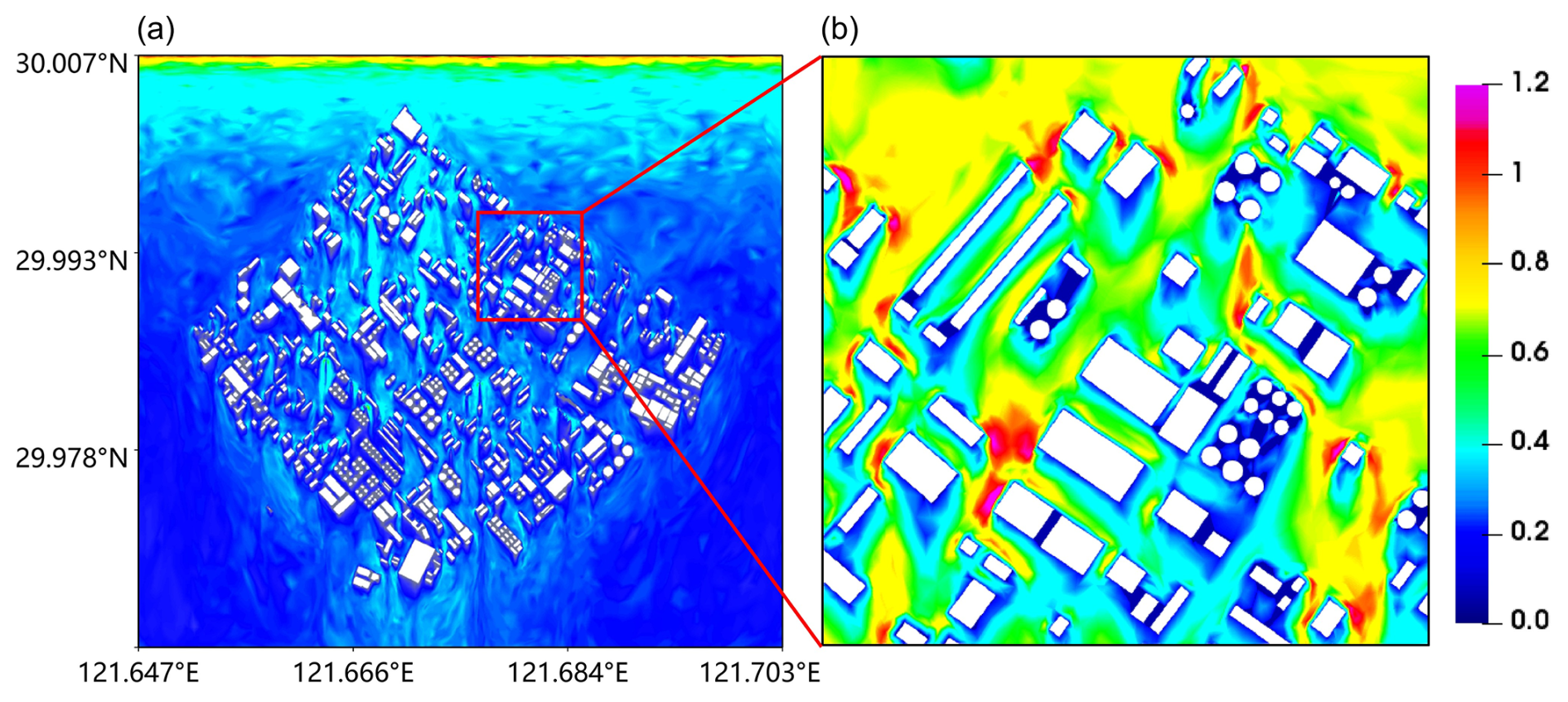
Figure 19Spatial distribution of the 10 m wind field magnitude (m s−1) simulated by FluidUrban 1.0 for the realistic urban scenario: (a) full-domain overview and (b) detailed subset of the region indicated in (a).
This study introduces and systematically evaluates FluidUrban v1.0, an advanced urban environmental modelling framework built upon the open-source Fluidity solver. The core methodological advancement of this research is the development of a dedicated 3D urban geometry and unstructured mesh generator, which is coupled with urban-specific boundary conditions. This integration establishes a robust foundation for explicitly resolving complex urban morphologies and driving the 3D DAMO algorithm. To comprehensively quantify the advantages of this adaptive framework, the model was validated against the high-fidelity WOTAN WTE datasets, investigating both urban flow and pollutant dispersion under varying surface roughness conditions and inflow directions. The principal findings of this study are summarized as follows:
-
Model Development and Initialisation: The integration of the newly developed geometry and mesh generator ensures that FluidUrban v1.0 can accurately initialize complex physical boundaries. During simulations, the DAMO algorithm effectively identifies evolving flow physics and pollutant concentration and dynamically refines or coarsens the computational grid, concentrating resources strictly in dynamically critical regions
-
Wind Speed Simulation: the DAMO framework consistently outperformed traditional non-uniform fixed meshes (FIXM) by capturing complex urban wind fields more accurately. On average, DAMO achieved a MAE of 0.187, significantly lower than the 0.214 obtained by FIXM. Performance gains were most pronounced in oblique inflow scenarios (M3), whereas under flow conditions parallel to street canyons, the difference in errors between the two methods was relatively small due to the higher stability of the flow gradients.
-
Wind Direction Simulation: the DAMO frame work showed a clear advantage in simulating local flow patterns and deflections around building structures. For realistic 30° tilted inflow conditions (M3), DAMO reduced the MAE of wind direction by 38.4 % in MR conditions and 36.1 % in HR conditions. This accuracy is attributed to the model's ability to automatically identify and refine mesh resolution at building corners and lateral separation regions where pressure gradients are highest.
-
Turbulence Intensity: The evaluation of velocity fluctuations revealed that FIXM severely underestimates turbulence across most heights due to the excessive numerical dissipation inherent in static pre-refinement. In contrast, DAMO dynamically resolves high-gradient regions, effectively limiting numerical diffusion. Consequently, DAMO preserves turbulent kinetic energy much more accurately, reproducing the vertical trends of streamwise (Iu) and lateral (Iv) turbulence intensities with a significantly reduced and tighter error distribution.
-
Pollutant Dispersion: DAMO successfully reproduced plume trajectories and the entrainment of pollutants into building-wake vortices. While fixed meshes often produced blurred boundaries and excessive numerical diffusion, the DAMO approach produced sharply defined plume contours and suppressed non-physical spreading. Quantitatively, the DAMO simulations achieved an 89 % compliance rate (16 out of 18) with established atmospheric model evaluation standards (FB, NMSE, and MG), significantly exceeding the 50 % compliance rate of FIXM simulations.
-
Accuracy-Efficiency Balance: Although DAMO introduces an additional normalized runtime cost, approximately 17.6 % in the current benchmark, due to the iterative mesh regeneration process, this overhead represents a necessary computational investment to achieve the demonstrated improvements in physical realism and multi-scale flow resolution. While the current benchmark primarily validates this physical fidelity, the theoretical cubic scaling behaviour of dynamic mesh adaptation suggests that this accuracy-efficiency trade-off will become increasingly favourable for ultra-large-scale urban domains, a premise that will be systematically explored in future work.
Beyond idealized benchmarks, the practical utility of the model was demonstrated through a realistic urban scenario simulation. The results confirm that FluidUrban v1.0 successfully resolves the pronounced spatial heterogeneity and complex channeling effects inherent to authentic city morphologies. By dynamically tracking flow evolution within dense building clusters and their downstream regions, the DAMO framework provides a high-fidelity representation of realistic urban ventilation patterns that are often unresolved by static mesh approaches. In conclusion, FluidUrban v1.0 proves to be a robust and highly accurate tool for resolving the transient, small-scale flow structures that dictate urban pollutant transport. By successfully maintaining sharp concentration gradients, the framework offers significant potential for high-fidelity exposure assessments in urban air quality studies. In its current scope, v1.0 is intentionally designed as an aerodynamic and scalar-transport baseline. Moving forward, future development will proceed in two main directions. First, we will continue to optimize the DAMO algorithm to further reduce runtime over complex building clusters. Second, to transition from a ventilation tool to a comprehensive urban model, we have already begun the integration of major urban physical components – including radiation, vegetation, and energy-balance physics. These extensions will be formally introduced in the upcoming FluidUrban v1.1. We acknowledge certain limitations in the current study. The present evaluation relies primarily on the WOTAN dataset and does not yet include additional standardized academic benchmarks such as the Compilation of Experimental Data for Validation of Micro-scale Dispersion Models (CEDVAL) or the Architectural Institute of Japan (AIJ) datasets, nor does it present a comprehensive parametric sensitivity analysis regarding adaptation frequency and error tolerance (ϵ). Furthermore, a strict fixed-accuracy comparison framework between DAMO and FIXM was not employed due to the challenges of pre-determining error distributions in transient LES. We plan to incorporate systematic mesh-convergence experiments and broader benchmark validations in our future work to comprehensively quantify the framework's performance limits. The combination of these future extensions with DAMO's capability to capture sharp thermal and chemical gradients will be essential for modeling urban multiscale physical processes and complex air quality events.
The FluidUrban v1.0 used in this study, a specialized derivative of the Fluidity framework, is archived on Zenodo (https://doi.org/10.5281/zenodo.19334189, Wu et al., 2026a). The 3D urban geometry and mesh generator, model output data reported in this paper, and the plotting scripts are archived on Zenodo (https://doi.org/10.5281/zenodo.22162054, Wu et al., 2026b). The wind-tunnel data is from Hamburg University (https://www.mi.uni-hamburg.de/en/arbeitsgruppen/windkanallabor/data-sets.html, last access: 8 May 2025).
The interactive computing environment is hosted on Zenodo (https://doi.org/10.5281/zenodo.22162054, Wu et al., 2026b). It provides a well-defined, self-contained structure for the data, code, text, documentation, runtime environment, and user-interface controls required to reproduce the results of this study. All necessary components for execution are included, and no additional assets need to be downloaded.
WX: Conceptualization, Data curation, Funding acquisition, Investigation, Methodology, Resources, Software, Supervision, Validation, Visualization, Writing (review and editing). CS: Conceptualization, Data curation, Formal analysis, Investigation, Methodology, Software, Visualization, Writing (original draft preparation). LJ: Data curation, Investigation, Validation, Writing (review and editing). ZY, WZ: Conceptualization, Project administration, Resources, Validation, Writing (review and editing). GP, ZJ: Software, Validation, Writing (review and editing). FF: Data curation, Investigation, Validation, Writing (review and editing).
The contact author has declared that none of the authors has any competing interests.
Publisher's note: Copernicus Publications remains neutral with regard to jurisdictional claims made in the text, published maps, institutional affiliations, or any other geographical representation in this paper. The authors bear the ultimate responsibility for providing appropriate place names. Views expressed in the text are those of the authors and do not necessarily reflect the views of the publisher.
Wu thanks for the technical support of the National Large Scientific and Technological Infrastructure “Earth System Numerical Simulation Facility” (grant no. 2025-EL-PT-000922, https://cstr.cn/31134.02.EL, last access: 30 July 2025) and wind-tunnel data support of Hamburg University (https://www.mi.uni-hamburg.de/en/arbeitsgruppen/windkanallabor/data-sets.html, last access: 8 May 2025).
This research has been supported by National Key Research and Development Program of China (grant no. 2023YFC3705702), the Chengdu Science and Technology Program (grant no. 2025-XT00-00001-GX), and the Engineering and Physical Sciences Research Council (EPSRC) (EP/X029093/1).
This paper was edited by Mohamed Salim and reviewed by three anonymous referees.
AMCG: Fluidity Manual, Applied Modelling and Computation Group, Imperial College London, Github [code], https://github.com/FluidityProject/fluidity (last access: 1 August 2025), 2014.
Apte, J. S. and Manchanda, C.: High-resolution urban air pollution mapping, Science, 385, 380–385, https://doi.org/10.1126/science.adq3678, 2024.
Arafa, M. A. and Zinat, A.: Comprehensive Validation of RANS-Based Urban Wind Flow Simulations using the `Michel-Stadt' Benchmark, J. Stud. Civil Eng., 2, 22–34, https://doi.org/10.53898/jsce2025222, 2025.
Badach, J., Dymnicka, M., and Baranowski, A.: Urban vegetation in air quality management: A review and policy framework, Sustainability, 12, 1258, https://doi.org/10.3390/su12031258, 2020.
Bauer, H. S., Muppa, S. K., Wulfmeyer, V., Behrendt, A., Warrach-Sagi, K., and Späth, F.: Multi-nested WRF simulations for studying planetary boundary layer processes on the turbulence-permitting scale in a realistic mesoscale environment, Tellus A, 72, 1–28, https://doi.org/10.1080/16000870.2020.1761740, 2020.
Connerton, P., Vicente de Assunção, J., Maura de Miranda, R., Dorothée Slovic, A., José Pérez-Martínez, P., and Ribeiro, H.: Air quality during COVID-19 in four megacities: lessons and challenges for public health, Int. J. Env. Res. Pub. He., 17, 5067, https://doi.org/10.3390/ijerph17145067, 2020.
COST Action ES1006: Best practice guidelines: Evaluation, improvement and guidance for the use of local-scale emergency prediction and response tools for airborne hazards in built environments, COST Action ES1006, ISBN 987-3-9817334-0-2, 2015.
Cui, P., Li, Z., and Tao, W.: Buoyancy flows and pollutant dispersion through different scale urban areas: CFD simulations and wind-tunnel measurements, Build. Environ., 104, 76–91, https://doi.org/10.1016/j.buildenv.2016.04.028, 2016.
da Silva, F. T., Reis Jr., N. C., Santos, J. M., Goulart, E. V., and de Alvarez, C. E.: The impact of urban block typology on pollutant dispersion, J. Wind Eng. Ind. Aerod., 210, 104524, https://doi.org/10.1016/j.jweia.2021.104524, 2021.
Di Sabatino, S., Buccolieri, R., and Salizzoni, P.: Recent advancements in numerical modelling of flow and dispersion in urban areas: a short review, Int. J. Environ. Pollut., 52, 172–191, https://doi.org/10.1504/IJEP.2013.058454, 2013.
Farrell, P. E., Piggott, M. D., Pain, C. C., Gorman, G. J., and Wilson, C. R.: Conservative interpolation between unstructured meshes via super mesh construction, Comput. Methods Appl. Mech. Engrg., 198, 2632–2642, https://doi.org/10.1016/j.cma.2009.03.004, 2009.
Franke, J., Hellsten, A., Schlunzen, K. H., and Carissimo, B.: The COST 732 Best Practice Guideline for CFD simulation of flows in the urban environment: a summary, Int. J. Environ. Pollut., 44, 419–427, https://doi.org/10.1504/IJEP.2011.038443, 2011.
Fuller, E. N., Schettler, P. D., and Giddings, J. C.: New method for prediction of binary gas-phase diffusion coefficients, Ind. Eng. Chem., 58, 18–27, https://doi.org/10.1021/ie50677a007, 1966.
Giani, P. and Crippa, P.: On the Sensitivity of Large-Eddy Simulations of the Atmospheric Boundary Layer Coupled with Realistic Large-Scale Dynamics, Mon. Weather Rev., 152, 1057–1075, https://doi.org/10.1175/MWR-D-23-0101.1, 2024.
Gkirmpas, P., Barmpas, F., Tsegas, G., Efthimiou, G., Tremper, P., Riedel, T., Vlachokostas, C., and Moussiopoulos, N.: An Evaluation of the Sensitivity of a Source Term Estimation Methodology of Sensor Configuration in an Urban-like Environment, Atmosphere, 15, 1512, https://doi.org/10.3390/atmos15121512, 2024.
Gromke, C.: A vegetation modeling concept for building and environmental aerodynamics wind tunnel tests and its application in pollutant dispersion studies, Environ. Pollut., 159, 2094–2099, https://doi.org/10.1016/j.envpol.2010.11.012, 2011.
Han, C., Hoose, C., Stengel, M., Coopman, Q., and Barrett, A.: Sensitivity of cloud-phase distribution to cloud microphysics and thermodynamics in simulated deep convective clouds and SEVIRI retrievals, Atmos. Chem. Phys., 23, 14077–14095, https://doi.org/10.5194/acp-23-14077-2023, 2023.
Hang, J., Luo, Z., Sandberg, M., and Gong, J.: Natural ventilation assessment in typical open and semi-open urban environments under various wind directions, Build. Environ., 70, 318–333, https://doi.org/10.1016/j.buildenv.2013.09.002, 2013.
Jackson, M. D., Percival, J. R., Mostaghimi, P., Tollit, B. S., Pavlidis, D., Pain, C. C., Gomes, J. L. M. A., El-Sheikh, A. H., Salinas, P., Muggeridge, A. H., and Blunt, M. J.: Reservoir modeling for flow simulation by use of surfaces, adaptive unstructured meshes, and an overlapping-control-volume finite-element method, SPE Reserv. Eval. Eng., 18, 115–132, https://doi.org/10.2118/163633-PA, 2015.
Khan, A., Vasilakopoulou, K., and Santamouris, M.: Exploring the potential impacts of anthropogenic heating on urban climate during heatwaves, Sci. Rep., 15, 3908, https://doi.org/10.1038/s41598-024-83918-y, 2025.
Khan, B., Banzhaf, S., Chan, E. C., Forkel, R., Kanani-Sühring, F., Ketelsen, K., Kurppa, M., Maronga, B., Mauder, M., Raasch, S., Russo, E., Schaap, M., and Sühring, M.: Development of an atmospheric chemistry model coupled to the PALM model system 6.0: implementation and first applications, Geosci. Model Dev., 14, 1171–1193, https://doi.org/10.5194/gmd-14-1171-2021, 2021.
Khomenko, S., Cirach, M., Pereira-Barboza, E., Mueller, N., Barrera-Gómez, J., Rojas-Rueda, D., de Hoogh, K., Hoek, G., and Nieuwenhuijsen, M.: Premature mortality due to air pollution in European cities: a health impact assessment, Lancet Planet. Health, 5, e121–e134, https://doi.org/10.1016/S2542-5196(20)30272-2, 2021.
Kurppa, M., Roldin, P., Strömberg, J., Balling, A., Karttunen, S., Kuuluvainen, H., Niemi, J. V., Pirjola, L., Rönkkö, T., Timonen, H., Hellsten, A., and Järvi, L.: Sensitivity of spatial aerosol particle distributions to the boundary conditions in the PALM model system 6.0, Geosci. Model Dev., 13, 5663–5685, https://doi.org/10.5194/gmd-13-5663-2020, 2020.
Kusaka, H., Ikeda, R., Sato, T., Iizuka, S., and Boku, T.: Development of a multi-scale meteorological large-eddy simulation model for urban thermal environmental studies: The “City-LES” model version 2.0, J. Adv. Model. Earth Sy., 16, e2024MS004367, https://doi.org/10.1029/2024MS004367, 2024.
Li, J., Li, Y., Wang, Z., Zhu, J., Kong, L., Li, J., Wu, H., Li, L., Tang, X., Cheng, Z., Zhang, L., Gan, P., Pan, X., Yang, W., Cao, K., and Zheng, J.: Next Generation Air Quality Models: Dynamical Mesh, New Insights into Mechanism, Datasets and Applications, Curr. Pollut. Rep., 11, 25, https://doi.org/10.1007/s40726-025-00355-9, 2025.
Li, J., Zheng, J., Zhu, J., Fang, F., Pain, C. C., Steppeler, J., Navon, I. M., and Xiao, H.: Performance of Adaptive unstructured Mesh Modeling in idealized Advection cases over steep Terrains, Atmosphere, 9, 444, https://doi.org/10.3390/atmos9110444, 2018.
Liang, W. and Zheng, X.: CFD simulation of mixed convection and pollutant dispersion in street canyons: A comparative assessment of LES, RANS, and SAS, Sustain. Cities Soc., 107126, https://doi.org/10.1016/j.scs.2026.107126, 2026.
Liu, W., Huang, Z., Sun, M., Zhang, H., Zhao, F., and Guo, R.: Applying Numerical Simulation to Identify the Suitable Block Scale for Improving Air Quality Inside Urban Streets, in: International Conference on Urban Climate, Sustainability and Urban Design, Springer, 603–616, https://doi.org/10.1007/978-981-97-8401-1_43, 2023.
Michel, S. J.: Feasibility Study of Heavy Gas Dispersion Experiments in Complex Environments in Physical Modeling, PhD thesis, Universität Hamburg, Hamburg, Germany, urn:nbn:de:gbv:18-ediss-111465, 2023.
Mottet, L., Song, J., Short, C. A., Chen, S., Wu, J., Yu, W., Xiong, J., Zhang, Q., Ge, J., Liu, M., Yao, R., and Li, B.: The hot summer-cold winter region in China: Challenges in the low carbon adaptation of residential slab buildings to enhance comfort, Energy Build., 223, 110181, https://doi.org/10.1016/j.enbuild.2020.110181, 2020.
Müller, A., Behrens, J., Giraldo, F. X., and Wirth, V.: Comparison between adaptive and uniform discontinuous Galerkin simulations in dry 2D bubble experiments, J. Comput. Phys., 235, 371–393, https://doi.org/10.1016/j.jcp.2012.10.038, 2013.
Nagai, T., Hibiya, T., and Syamsudin, F.: Direct estimates of turbulent mixing in the Indonesian archipelago and its role in the transformation of the Indonesian throughflow waters, Geophys. Res. Lett., 48, e2020GL091731, https://doi.org/10.1029/2020GL091731, 2021.
Nonaka, I. T.: Modeling and simulation of multicomponent evaporative sprays in generic conditions, Master's thesis, Universidade Federal de Uberlândia, Faculdade de Engenharia Mecânica, Uberlândia, Brazil, https://doi.org/10.14393/ufu.di.2025.5579, 2025.
Pain, C. C., Umpleby, A. P., de Oliveira, C. R. E., and Goddard, A. J.: Tetrahedral mesh optimisation and adaptivity for steady-state and transient finite element calculations, Comput. Meth. Appl. Mech. Eng., 190, 3771–3796, https://doi.org/10.1016/S0045-7825(00)00294-2, 2001.
Pain, C. C., Piggott, M. D., Goddard, A. J. H., Fang, F., Gorman, G. J., Marshall, D. P., Eaton, M. D., Power, P. W., and de Oliveira, C. R. E.: Three-dimensional unstructured mesh ocean modeling, Ocean Model., 10, 5–33, https://doi.org/10.1016/j.ocemod.2004.07.005, 2005.
Park, S. J. and Kim, J. J.: Development of a computational fluid dynamics model adopting a nested grid system: Flow simulations for ideal and real urban settings, Urban Clim., 53, 101801, https://doi.org/10.1016/j.uclim.2023.101801, 2024.
Pavlidis, D., Gorman, G., Gomes, J., Pain, C., and ApSimon, H.: Synthetic-eddy method for urban atmospheric flow modelling, Bound.-Lay. Meteorol., 136, 285–299, https://doi.org/10.1007/s10546-010-9508-x, 2010.
Pesci, C., Weiner, A., Marschall, H., and Bothe, D.: Computational analysis of single rising bubbles influenced by soluble surfactant, J. Fluid Mech., 856, 709–763, https://doi.org/10.1017/jfm.2018.723, 2018.
Power, P. W., Piggott, M. D., Fang, F., Gorman, G. J., Pain, C. C., Marshall, D. P., Goddard, A. J. H., and Navon, I. M.: Adjoint goal-based error norms for adaptive mesh ocean modelling, Ocean Model., 15, 3–38, https://doi.org/10.1016/j.ocemod, 2006.
Ricci, A., Kalkman, I., and Blocken, B.: Local-scale forcing effects on wind flows in an urban environment: Impact of geometrical simplifications, J. Wind Eng. Ind. Aerodyn., 170, 238–255, https://doi.org/10.1016/j.jweia.2017.08.001, 2017.
Savre, J., Percival, J., Herzog, M., and Pain, C.: Two-dimensional evaluation of ATHAM-fluidity, a nonhydrostatic atmospheric model using mixed continuous/discontinuous finite elements and anisotropic grid optimization, Mon. Weather Rev., 144, 4349–4372, https://doi.org/10.1175/MWR-D-15-0398.1, 2016.
Schalau, S., Habib, A., and Michel, S.: A modified k-ϵ turbulence model for heavy gas dispersion in built-up environment, Atmosphere, 14, 161, https://doi.org/10.3390/atmos14010161, 2023.
Sezen, S. and Atlar, M.: An alternative Vorticity based Adaptive Mesh Refinement (V-AMR) technique for tip vortex cavitation modeling of propellers using CFD methods, Ship Technol. Res., 69, 1–21, https://doi.org/10.1080/09377255.2021.1927590, 2022.
Tarraf, A., Schreiber, M., Cascajo, A., Besnard, J.-B., Vef, M.-A., and Huber, D.: Malleability in modern HPC systems: current experiences, challenges, and future opportunities, IEEE Trans. Parallel Distrib. Syst., 35, 1551–1564, https://doi.org/10.1109/TPDS.2024.3406764, 2024.
Tominaga, Y., Mochida, A., Yoshie, R., Kataoka, H., Nozu, T., Yoshikawa, M., and Shirasawa, T.: AIJ guidelines for practical applications of CFD to pedestrian wind environment around buildings, J. Wind Eng. Ind. Aerodyn., 96, 1749–1761, https://doi.org/10.1016/j.jweia.2008.02.058, 2008.
Turker, M. and Koc-San, D.: Building extraction from high-resolution optical spaceborne images using the integration of support vector machine (SVM) classification, Hough transformation and perceptual grouping, Int. J. Appl. Earth Obs. Geo., 34, 58–69, https://doi.org/10.1016/j.jag.2014.06.016, 2015.
United Nations: Department of Economic and Social Affairs, Population Division, World Urbanization Prospects: The 2018 Revision (ST/ESA/SER.A/420), United Nations, New York, https://doi.org/10.18356/b9e995fe-en, 2019.
VDI: Environmental meteorology – Physical modelling of flow and dispersion processes in the atmospheric boundary layer – Application of wind tunnels,VDI Standard 3783 Blatt 12, Verein Deutscher Ingenieure, Düsseldorf, 2000.
Wang, C., Wang, W., Qu, J., Wang, Q., Wang, X., and Liu, X.: Multi-Scale Validation of CFD Simulations for Pollutant Dispersion Around Buildings, Processes, 13, 4076, https://doi.org/10.3390/pr13124076, 2025.
Weger, M. and Heinold, B.: Air pollution trapping in the Dresden Basin from gray-zone scale urban modeling, Atmos. Chem. Phys., 23, 13769–13790, https://doi.org/10.5194/acp-23-13769-2023, 2023.
Wu, X., Abubakar-Waziri, H., Fang, F., Dilliway, C., Wu, P., Li, J., Yao, R., Bhavsar, P., Kumar, P., Pain, C. C., and Chung, K. F.: Modeling for understanding of coronavirus disease-2019 (COVID-19) spread and design of an isolation room in a hospital, Phys. Fluids, 35, 025111, https://doi.org/10.1063/5.0135247, 2023.
Wu, X., Chen, S., and Fang, F.: FluidUrban v1.0, Zenodo [code], https://doi.org/10.5281/zenodo.19334189, 2026a.
Wu, X., Chen, S., Li, J., Zhang, Y., Wang, Z., Gan, P., Zheng, J., and Fang, F.: FluidUrban v1.0: Enhancing Urban Ventilation and Pollutant Dispersion Modelling with Three-dimensional Dynamic Adaptive Meshes Optimization (Version 2.0), Zenodo [data set], https://doi.org/10.5281/zenodo.22162054, 2026b.
Yang, L., Wang, G., Wang, Y., Wang, Y., Ma, Y., and Zhang, X.: A rapid computational method for quantifying inter-regional air pollutant transport dynamics, Atmosphere, 16, 163, https://doi.org/10.3390/atmos16020163, 2025.
Yu, J., Lyu, H., Xu, R., Ouyang, W., and Liu, X.: Flow2Mesh: A flow-guided data-driven mesh adaptation framework, Phys. Fluids, 36, https://doi.org/10.1063/5.0188690, 2024.
Zhang, C. X., Liu, Y., Fu, B. S., and Yu, X. J.: Direct numerical simulation of subsonic–supersonic mixing layer, Acta Astronaut., 153, 50–59, https://doi.org/10.1016/j.actaastro.2018.10.004, 2018.
Zheng, J., Zhu, J., Wang, Z., Fang, F., Pain, C. C., and Xiang, J.: Towards a new multiscale air quality transport model using the fully unstructured anisotropic adaptive mesh technology of Fluidity (version 4.1.9), Geosci. Model Dev., 8, 3421–3440, https://doi.org/10.5194/gmd-8-3421-2015, 2015.
Zheng, J., Wu, X., Fang, F., Li, J., Wang, Z., Xiao, H., Zhu, J., Pain, C., Linden, P., and Xiang, B.: Numerical study of COVID-19 spatial–temporal spreading in London, Phys. Fluids, 33, https://doi.org/10.1063/5.0048472, 2021.
Zhong, J., Liu, J., Xu, Y., and Liang, G.: Pedestrian-level gust wind flow and comfort around a building array–Influencing assessment on the pocket park, Sustain. Cities Soc., 83, 103953, https://doi.org/10.1016/j.scs.2022.103953, 2022.
- Abstract
- Introduction
- Methodology
- Validation results based on WTE datasets
- Realistic urban scenario simulation
- Conclusions
- Code and data availability
- Interactive computing environment (ICE)
- Author contributions
- Competing interests
- Disclaimer
- Acknowledgements
- Financial support
- Review statement
- References
- Abstract
- Introduction
- Methodology
- Validation results based on WTE datasets
- Realistic urban scenario simulation
- Conclusions
- Code and data availability
- Interactive computing environment (ICE)
- Author contributions
- Competing interests
- Disclaimer
- Acknowledgements
- Financial support
- Review statement
- References