
the Creative Commons Attribution 4.0 License.
the Creative Commons Attribution 4.0 License.
 | 17 Nov 2026
The stippled grid points are statistically significant: (mis)uses of false discovery rate correction for geospatial data
Michael Konrad Schutte

Leonardo Olivetti
Flavio Maria Emanuele Pons
Gabriele Messori
Peer-reviewed articles in the geosciences routinely assess statistical significance in spatially distributed data. Statistical significance is often assessed independently at each grid point, while formal adjustment for multiple testing is applied less consistently. Although several approaches to account for multiple testing exist, their application to geosciences data is not always straightforward, as these data often exhibit spatially coherent signals.
In this work we revisit the Benjamini-Hochberg (BH) false discovery rate (FDR) correction, which is a commonly used method to account for multiple testing, in the context of spatially structured datasets. We first highlight how neglecting multiple-testing correction can substantially inflate the number of false positives. We further show that the BH correction approach proposed in literature for application in geosciences can yield counterintuitive results when applied to spatially coherent signals that cover large fractions of a spatial domain. To illustrate the latter point, we provide an example based on near-surface air temperature composites following sudden stratospheric warmings. We show that when anomalies are spatially coherent, restricting the spatial domain can increase the BH-corrected significance threshold. Consequently, the same underlying field can display a larger number of statistically significant grid points solely due to domain selection, despite unchanged data. We explain this behavior from the point of view of the rank-based structure of the BH correction and discuss its implications for spatial inference and uncertainty quantification in the geosciences. Furthermore, a numerical experiment confirms that the larger the fraction of true positives the higher the BH-corrected significance threshold becomes for a set FDR level.
Building on these insights, we outline practical recommendations for transparent and robust significance assessment in geoscientific applications. These include clearly documenting multiple-testing corrections when adjusted pointwise significance is shown, cautious interpretation of adjusted thresholds, careful avoidance of a posteriori domain selection and considering spatially aware alternatives such as regional or cluster-based inference when appropriate. Overall, our results highlight both the need to account for multiple-testing, and potential issues with a naïve application and interpretation of the BH correction. We hope that our work may contribute to more robust statistical testing in the geosciences.
- Article
(5700 KB) - Full-text XML
- BibTeX
- EndNote


Highlighting regions with statistically significant signals on maps is very common in the analysis of geospatial data, including model-evaluation, observational diagnostics and event composites (e.g., Deser et al., 2012; Eade et al., 2014; Butler et al., 2017). This approach supports hypothesis testing and interpretation of results, and can also translate into real-world decision-making, e.g., in the case of forecast evaluation (e.g., Jeuring et al., 2024; Pappenberger et al., 2019; Taggart and Wilke, 2025). However, the common practice of applying a pointwise significance test at each data point (i.e. repeated local tests) introduces a fundamental statistical issue: when hypothesis tests are conducted multiple times, the probability of finding apparently significant results purely by chance increases sharply. For example, if 100 independent grid points are tested at the 5 % significance level, one would expect on average five points to appear “significant” even in the absence of any true signal (i.e. false rejections of the null hypothesis). However, for any single sample, this number may be higher. The expected proportion of incorrectly rejected null hypotheses among all rejected hypotheses is known as false discovery rate (FDR). Moreover, the chance of at least one spurious rejection is extremely high: 99.41 % when performing 100 local tests. This point was eloquently made by Wilks (2016). The geosciences community has been aware of this issue for well over a century (Walker, 1914) and the issue has since been revisited regularly (e.g., Livezey and Chen, 1983; Katz and Brown, 1991; Katz, 2002; Wilks, 2006, 2016).
To avoid inflating the number of false rejections, adjustment for multiple testing is required. A variety of approaches have been proposed to address this issue, including Family-Wise Error Rate (FWER) control (e.g., Walker, 1914), field significance methods (e.g., Livezey and Chen, 1983) and, more recently, the Benjamini–Hochberg FDR correction (Benjamini and Hochberg, 1995), hereinafter BH correction. The BH correction aims to limit the expected proportion of falsely rejected hypotheses among all tests, and is widely applied in many fields such as genomics or neuroimaging (e.g., Noble, 2009; Alberton et al., 2020). The original paper by Benjamini and Hochberg (1995) has accumulated more than 125 000 citations according to Google Scholar. Following the review and recommendations of Wilks (2016), the BH correction has also become the de facto gold standard for multiple-testing correction in geoscientific applications. Nonetheless, it is still implemented sporadically in the field. To provide a heuristic illustration we randomly sampled fifty articles from meteorology and climate science cited by the IPCC Sixth Assessment Report, Chapter 11 (Seneviratne et al., 2021), which discusses how anthropogenic climate change affects weather and climate extreme events. We found that 18 studies assessed statistical significance on a map, of which 17 without multiple-testing correction, while only one article implemented FDR correction. These numbers are consistent with previous empirical observations of the same issue (e.g., Wilks, 2016) and further motivate recent efforts to implement FDR correction methods in climate model testing (Kelleher and Mahajan, 2026).
However, even the application and interpretation of the BH correction can be problematic. The BH correction is often misunderstood as adjusting the significance threshold for each individual grid point, making it “harder” for a point to be considered significant. The last author of this study has himself implicitly adopted this fallacious interpretation in some of his past work. While BH correction does control the global error rate, it does not provide any guarantee for individual grid points. In some applications, the resulting BH-corrected threshold may even be higher than the uncorrected threshold, if the pointwise significance level is lower than the chosen FDR level. That is, some grid points become significant only after the BH correction. This effect is highly sensitive to the choice of domain. Interpreting BH-corrected significance on maps as if each highlighted grid point were locally significant can therefore be misleading.
There exist adaptive refinements of the BH correction that adapt to properties of the data, either by estimating the proportion of true null hypotheses to increase power (Storey, 2002; Benjamini et al., 2006), or by modifying the procedure to remain valid under dependence between tests (Benjamini and Yekutieli, 2001; Mrkvička and Myllymäki, 2023). However, we leave a deeper analysis of their behavior to future work. Indeed, Cortés et al. (2020) found that the BH correction still outperforms the method developed by Benjamini and Yekutieli (2001) that accounts for test dependence. Moreover, the comparatively limited application of FDR corrections in the geosciences speaks for focusing on the BH correction, which offers the best trade-off among effectiveness, simplicity, and established use in the field.
In the following section, we provide a more detailed explanation of the BH correction, and subsequently highlight that: (i) any depiction of pointwise statistical significance on maps must be accompanied by an explicit and appropriate multiple-testing correction; and (ii) the BH correction can yield misleading thresholds if misunderstood or deliberately exploited. We illustrate these points with an example based on meteorological reanalysis data and a numerical experiment. Finally, we conclude with some practical recommendations for transparent and robust significance testing in the geosciences and its interpretation.
Under the assumption of independent tests, the number of falsely rejected null hypotheses is a random variable following a binomial distribution with probability α, the chosen significance level (Wilks, 2016). Consequently, the probability of obtaining at least one false positive approaches unity as the number of tests increases. For the commonly used 5 % significance level, the probability of no false rejections is (1−0.05)n, where n is the number of tests. In high-resolution gridded maps containing thousands of grid points, at least one false rejection is therefore almost certain. Moreover, the expected number of false rejections scales linearly with n (the expected value of the binomial distribution is n⋅α), implying that hundreds of spuriously significant grid points may appear in a single high-resolution map (e.g., on average about 500 for n=10 000 grid points).
A commonly-used approach in the geosciences to address this issue is the BH correction (Benjamini and Hochberg, 1995) for FDR, which seeks to limit the expected proportion of falsely rejected hypotheses. For example, an FDR level of αFDR=0.1 implies that, on average, no more than 10 % of rejected null hypotheses are false positives. In practice, the p values from the local tests are first sorted in ascending order and the BH-corrected threshold is defined as
so that all p values smaller than or equal to the largest p value satisfying this condition are considered statistically significant. If no local p value satisfies this condition, the field as a whole does not reach statistical significance, implying that all apparent local discoveries may be spurious – an interpretation analogous to that of field significance tests. Following Eq. (1), controlling FDR means that the threshold adjusts dynamically depending on the proportion of low p values in the sample. While this property is intrinsic to the BH correction, it is seldom acknowledged when applied in practice.
The appeal of the BH correction for geoscientific applications lies primarily in its ease of implementation and apparent ease of interpretation, as well as its robustness to violations of the assumption that local tests are independent (Wilks, 2016). Indeed, while the BH correction assumes local test independence, numerical experiments by Wilks (2016) show that the correction performs well even in the presence of strong spatial autocorrelation – as is commonly the case in many geophysical fields. This contrasts earlier approaches such as field significance testing, which are highly sensitive to spatial dependence (Livezey and Chen, 1983).
However, while the BH correction provides a valid control of the global error rate, it does not necessarily render individual tests more conservative in a local sense. Based on simulations with spatially autocorrelated data, Wilks (2016) recommends selecting an αFDR approximately twice as large as the target field significance level in order to avoid overly restrictive thresholds. This recommendation is well-motivated for large-scale maps in which statistically significant signals are sparse and spatially restricted, yet it exposes an important limitation of the BH correction. Because the BH-corrected threshold depends on the rank ordering of local p values, it can become counterintuitively permissive when applied to a spatial subset exhibiting a prevalent signal. In practice, selecting an αFDR larger than the nominal pointwise significance level (e.g., αFDR=0.1 for a target field significance level of 5 % as recommended by Wilks, 2016) can lead to corrected thresholds that exceed said pointwise significance level. Applications in the geosciences literature often implicitly or explicitly assume that the BH correction makes the test more stringent, without acknowledging that commonly-used parameter choices may produce the counterintuitive outcome that more grid points appear statistically significant on a map following BH correction than when using uncorrected local tests. This becomes particularly problematic if the BH correction is applied a posteriori, after inspecting the results of uncorrected grid-point-level tests, in which case it may be regarded as p-hacking.
The BH correction operates by controlling a set-level property of the rejected hypotheses, rather than adjusting the error probability at each grid point. When BH-corrected results are visualized in the same manner as pointwise significance maps, this distinction is easily obscured, encouraging local interpretations that the method does not support. In contrast to pointwise testing, which bounds the probability of false positives at each location, the BH correction constrains only the expected fraction of false positives among all declared discoveries. As a result, FDR-based significance should not be interpreted as a local measure of statistical significance. This point is illustrated with a real-world case study in the next section.
We now illustrate how the BH correction can yield corrected thresholds that exceed the nominal local significance level, and how markedly different apparent patterns of statistical significance can result from the same underlying data, solely as a consequence of changing the analysis domain. This is what would occur if the domain were selected a posteriori after inspecting the results. Employing an example from meteorology, we show composites of 2 m air temperature (t2m) anomalies, averaged over the 60 d following 26 Sudden Stratospheric Warming events (SSWs; e.g., Baldwin et al., 2021; Lee et al., 2025). It is well documented that SSWs often result in near-surface responses, for instance showing below-average temperatures over northern Eurasia (e.g., Kolstad et al., 2010; Butler et al., 2017). However, considerable uncertainty remains about the exact location and magnitude of these anomalies due to variability in stratosphere-troposphere coupling (e.g., Oehrlein et al., 2021; Kolstad et al., 2022). In the following, we illustrate how domain choice affects the visual interpretation of statistical significance in this example.
3.1 Temperature data and p value computation
The temperature data is obtained from ERA5 reanalysis (Hersbach et al., 2020), a widely used data set in meteorology. We use t2m data over the Northern Hemisphere north of 20° N with a horizontal resolution of 0.5° between 1980 and 2022. After linearly detrending the t2m data, temperature anomalies are computed by subtracting a smoothed seasonal cycle (15 d centered running mean). The 26 SSW dates between 1980 and 2022 are obtained from the Sudden Stratospheric Warming Compendium (Butler et al., 2017; Butler, 2025), based on the conventional definition of reversal of 10 hPa zonal winds at 60° N (Charlton and Polvani, 2007).
To test the statistical significance of the t2m anomalies, we assess at each grid point whether the mean of the 26 individual 60 d mean t2m anomalies following the SSW onset dates is significantly colder than climatology using a one-sided, one-sample Student's t test:
where and s are the sample mean and sample standard deviation of the n=26 individual event-wise 60 d mean anomalies at a given grid point, and μ0=0 is the population mean under the null hypothesis of no SSW-related response, consistent with the detrended and deseasonalized nature of the input data. The resulting p value is obtained from the Student's t-distribution with degrees of freedom, testing the alternative hypothesis that the mean anomaly is significantly colder than climatology (). The 60 d time window follows observational and modeling evidence that SSWs influence tropospheric circulation for up to 60 d after their onset (e.g., Baldwin and Dunkerton, 2001; Oehrlein et al., 2021). We note that temperature variability is not stationary across the November–March window, such that individual SSW events falling in different months are drawn from different background-variability regimes. While this introduces mild heterogeneity in the pooled sample variance estimate, it does not affect the domain-dependence of the BH-corrected threshold illustrated below, which is a structural property of the BH correction.
3.2 Statistical significance assessment
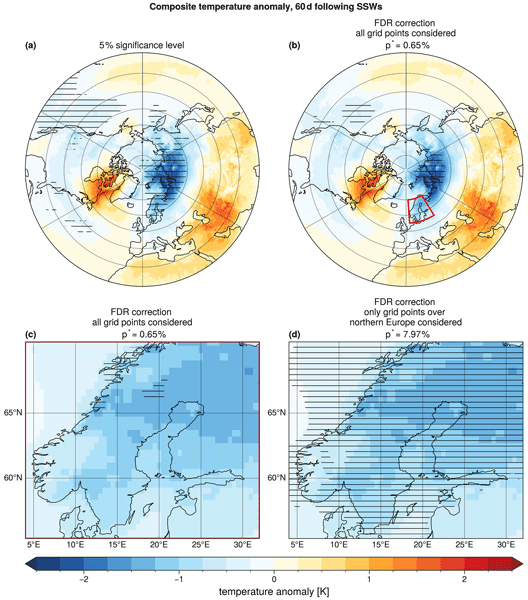
Assessing statistical significance with independent tests for a 5 % threshold at each grid point highlights broad regions of significant cold temperature anomalies (Fig. 1a). Even relatively weak anomalies, for example over the North Atlantic or over North America, are marked as statistically significant. Regardless of the lower temperature variability over oceans than over land, one may suspect that the significance of some signals is spurious.

Figure 1Composites of 2 m air temperature anomalies averaged over 60 d following SSWs. Statistical significance of cold anomalies is indicated by horizontal hatching for all grid points north of 20° N with respect to: (a) A local 5 % significance level using a one-sided Student's t test and (b) adjusted with the BH correction. Panel (c) shows the same hatching as in the red box in panel (b), while panel (d) shows horizontal hatching for the BH-corrected significance with respect to only northern European grid points. The subtitles in panels (b) to (d) further indicate the BH-corrected p value as p*. A zoomed-in map of northern Europe for the local 5 % significance level is found in Fig. A2.
Applying the BH correction as recommended by Wilks (2016) with α=0.1 to all grid points between 20 and 90° N reduces the number of points marked as statistically significant (Fig. 1b). In agreement with earlier studies, northern Eurasia stands out as the region with the clearest signal of significant below-average temperatures following SSWs (e.g., Kolstad et al., 2010; Butler et al., 2017). In this case, the BH correction suppresses points with relatively weak anomalies, as these points could be linked to false rejections, while retaining the signal with the highest amplitude over northern Eurasia.
We now restrict our attention to t2m anomalies over northern Europe (55–70° N, 4–32° E; Fig. 1c), which has been highlighted as a region experiencing colder than usual temperatures following SSWs in a number of studies (e.g., King et al., 2019; Kolstad et al., 2010; Monnin et al., 2022). We note that this domain was identified partly through inspection of the hemispheric composite in Fig. 1b, which is an a posteriori choice of the kind our study cautions against, and one that here serves as an example of the issue we aim to highlight. The behavior described below is moreover qualitatively consistent for other regions (e.g., Fig. A1). If the BH correction is applied only to grid points within northern Europe, the cold anomalies over nearly the entire region appear statistically significant (Fig. 1d). This is in sharp contrast to the case where the BH correction is applied on the full hemispheric analysis domain (cf. Fig. 1c and d). The number of hatched grid points in the former case is even larger than the uncorrected significance testing case (cf. Figs. 1d to A2), which is linked to the pointwise significance level of 5 % being lower than the FDR level α=0.1. The discrepancy occurs even though the underlying temperature anomaly field is identical in all cases. It arises from the dependence of the BH-corrected threshold on the rank ordering of p values. Restricting the analysis to a region dominated by low p values increases the adjusted threshold, allowing a larger fraction of points to satisfy the corrected value.
To better understand this behavior, we examine the ranked p values and corresponding thresholds of negative t2m anomalies (Fig. 2). When the BH correction is applied to all grid points between 20 and 90° N, the intersection defining p* (Eq. 1) is found at %, well below 5 % (Fig. 2a). In contrast, when the BH correction is applied only to northern Europe, % is an order of magnitude higher (Fig. 2b). This difference arises because the p values over northern Europe are generally small, increasing the fraction of points below the line when fewer grid points are considered. While the absolute distribution of p values over northern Europe remains unchanged, their relative ranks within the smaller test family differ, resulting in a substantially more permissive threshold.

Figure 2Ranked p values (colored line) and the BH-corrected threshold (black line) for: (a) all grid points north of 20° N (Fig. 1b) and (b) northern Europe only (Fig. 1d). In both panels, the red dotted line indicates the significance threshold obtained from the respective FDR correction, and the black dashed line indicates the 5 % significance level. Histograms to the right of each panel show the distribution of p values. Note that both panels only show p values below 0.14 for improved readability. Figure A3 shows all p values, including those above 0.14.
The example above illustrates that the BH correction as commonly implemented in geoscience applications can yield less restrictive thresholds than the uncorrected statistical test when applied to spatial domains dominated by coherent signals. This behavior follows directly from the choice of α=0.1 being larger than the pointwise significance level of 5 % and from the way the BH correction is defined (Benjamini and Hochberg, 1995), which identifies the critical p value threshold p* as the largest p value satisfying Eq. (1).
When only a small fraction of p values in the full set are sufficiently low, the BH criterion is satisfied only at relatively early ranks in the ordered p value distribution, resulting in a comparatively strict (low) threshold. Conversely, when the analysis is restricted to a domain dominated by sufficiently small p values, the ratio changes so that the intersection occurs at a higher p value, effectively relaxing the threshold for declaring significance. In other words, the same underlying field can yield an apparently higher fraction of grid points identified as statistically significant on a reduced spatial domain than both the BH correction applied to a larger domain and the uncorrected case.
Crucially, this behavior reflects a fundamental tension between a set-level error criterion and the local interpretation encouraged by significance maps. Coherent anomalies, such as large-scale temperature responses, generate clusters of similar p values that alter the rank structure on which the BH correction operates. This behavior only applies to domains with a relatively large proportion of small p values and when αFDR is larger than the nominal pointwise significance level. If either of these conditions does not hold, the BH correction has the more intuitive effect of reducing or leaving unchanged the significance threshold p*. While this FDR control method remains valid under many forms of spatial dependence, its sensitivity to rank ordering implies that spatial context and domain choice can strongly influence the resulting significance threshold, and hence the apparent robustness and spatial extent of detected signals.
To complement the meteorological example and investigate the sensitivity of the BH-corrected threshold to key properties of the tested field in a controlled setting, we conduct a numerical experiment with synthetic data. We mainly consider the role of the fraction of the true signal fs, but also include sensitivity analysis to other parameters such as the relationship between the domain size and the correlation length in the data, and the signal-to-noise ratio (SNR).
5.1 Experimental design
We generate synthetic fields on a square grid with grid points. The background field has value 0. Similar to Wilks (2016), the signal consists of a circular patch of grid points with value 1, occupying a fraction fs of the total domain, defined by the radius . A circular patch provides a geometrically simple and parameter-free signal region that can be scaled through fs, making it straightforward to control the fraction of the true signal. Values of fs ranging from 0.01 to 0.9 (Table 1) span the full range from a sparse, localized signal broadly analogous to the hemispheric case in Sect. 3.2 where only a small fraction of grid points exhibit relatively strong anomalies, to a spatially dominant response analogous to the northern Europe subdomain where most grid points carry relatively small p values.
Table 1Summary of parameter values used in the numerical experiment.
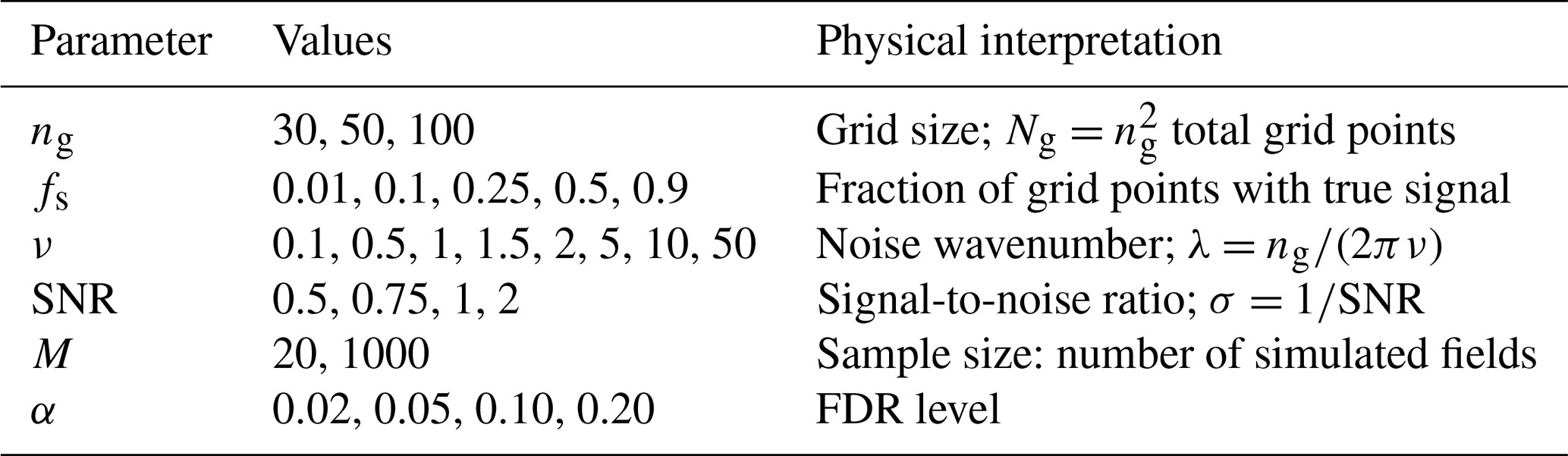
To this signal we add a spatially correlated Gaussian noise field with standard deviation , so that larger SNR values correspond to stronger signals relative to the background variability. Gaussian noise is a natural and widely used choice for synthetic geophysical fields, as many atmospheric variables are approximately normally distributed after removing the seasonal cycle (von Storch and Zwiers, 1999; Wilks, 2011). It is furthermore consistent with the distributional assumptions underlying the Student's t test used to compute local p values, and provides a tractable, analytically well-understood null field. Spatial correlation is introduced by generating white noise in spectral space and multiplying each Fourier mode by a spectral filter before transforming back to physical space, yielding a field with power spectral density , where is the radial wavenumber, and ν is the noise wavenumber, corresponding to a spatial autocorrelation length of approximately . Implementing the correlation structure in the spectral space provides exact and independent control over the power at each wavenumber, which is not achievable with smoothing kernels in the physical space, where the resulting spectral properties are determined implicitly by the kernel shape and width. The noise wavenumber ν used in the numerical experiment spans from large-scale structures (ν=0.1, λ≈1.6ng) to near-white noise (ν=50, λ≈0.003ng), covering the range from planetary-scale to grid-scale spatial dependence typical of geophysical fields.
The parameter values explored in the experiment are summarized in Table 1. For each of the 480 parameter combinations of Ng, fs, ν and SNR, we generate M independent realizations of the field, each consisting of the same deterministic signal and a newly drawn noise field. These realizations take the role of the individual events or ensemble members in a real application, such as the 26 SSW events in Sect. 3. At each grid point, M simulated values form the sample entering the significance test described below.
We consider two sample sizes for M. For M=1000 (all realizations), the signal is separated from the noise by a wide margin at the signal grid points (for SNR=0.5, the expected t-statistic is about 16), so that the dependence of the BH-corrected threshold on the signal fraction can be studied independently of limited detection power. A single test is performed per parameter combination, so the spread across combinations reported below reflects parameter variability. For M=20, closer to typical sample sizes in geoscientific composite and ensemble analyses, detection power is limited. To quantify the sampling variability in this low-power regime (SNR=0.5, M=20), the test is repeated for 100 random subsets of 20 realizations, drawn without replacement from the 1000 realizations, for every combination of the remaining parameters (Ng, fs, ν).
At each grid point, we test the null hypothesis that the mean over the M simulated values is zero against the alternative that it is larger than zero, using the one-sided, one-sample Student's t-test of Eq. (2) with n=M, as in the SSW example (Sect. 3). As the simulated fields are independent and the noise is Gaussian, the assumptions of the t-test hold at each grid point by construction. The spatial correlation of the noise affects only the dependence between the tests. The resulting p values are corrected with the BH procedure (Eq. 1) for four different FDR levels, spanning values from below to above the standard recommendation of Wilks (2016).
To evaluate the behavior of the BH correction across this parameter space, we record for each application of the test and BH correction (i.e., each parameter combination for M=1000 and each of the 100 subsets for M=20) the identified threshold p* (obtained as in Sect. 3), and the number of true signal grid points correctly (TP) and background grid points incorrectly (FP) flagged as significant. From these we compute the realized false discovery proportion,
and power,
where Nsig is the total number of true signal grid points in the domain.
5.2 Numerical results
We now summarize the sensitivity of the three diagnostics as a function of signal fraction fs.
The BH-corrected significance threshold p* increases monotonically with fs and is higher for larger α (Fig. 3a). This directly reproduces in a controlled setting the mechanism illustrated by the meteorological example: as the fraction of truly significant grid points grows, the rank-based threshold becomes more permissive. For fs≲0.1, p* remains well below the 5 % local significance level across all α choices, while for fs>0.1 the BH-corrected threshold p* can substantially exceed the 5% level, particularly for larger α. For the low-power regime, BH-corrected significance thresholds are consistently lower than in the full parameter space but follow the same dependence on fs.

Figure 3Results of the numerical experiment as a function of signal fraction fs. Panels (a)–(c) show the median (markers) and interquartile range (error bars) of the BH-corrected threshold p*, the realized false discovery proportion (FDP), and power, respectively, aggregated across all 480 parameter combinations with M=1000 (saturated lines) and across the low-power regime (SNR=0.5, M=20; pale). Panel (d) shows the FDP–Power trade-off as a scatter plot, with markers indicating the median and error bars the interquartile range across all combinations (solid) and the low-power regime (pale). Colors indicate the choice of FDR level α as provided in the legend in panel (a). In panel (c), the median power across all parameter combinations is shown as a single gray line, as all choices of α yield near-identical power close to unity.
FDP is approximately constant across low-to-moderate signal fractions and decreases for larger signal fractions (Fig. 3b), reflecting the increasing dominance of true positives among all rejections as the signal covers a larger portion of the domain. This pattern is consistent across both the full parameter space and the low-power regime (SNR=0.5, M=20), confirming that it is a property of the BH correction method rather than an artifact of specific parameter choices.
Power is close to unity in most parameter combinations (Fig. 3c), indicating that for typical settings all choices of α achieve near-perfect detection. This is expected for M=1000, where signal grid points yield p values far below the BH threshold for all α (Sect. 5.1). Furthermore, the high power may be related to the sharp signal boundary in the experimental setup, which yields in several cases well-separated p value distributions for signal and background grid points. In the low-power regime, however, power rises from near zero at fs=0.01 to between about 0.3 (α=0.02) and 0.9 (α=0.2) at fs=0.9, and is higher for larger α (Fig. 3c). A more permissive FDR level raises p* and thus admits more rejections, which increases power but also the realized FDP. When the signal is weak compared to the noise and the sample is small, the p values of signal and background grid points overlap, so that detecting more signal points inevitably comes at the cost of more false positives.
The FDP–power trade-off (Fig. 3d) is consistent with the results for FDP and power discussed before: in the case of M=1000, all α choices achieve near-perfect power and the meaningful distinction between them lies in FDP control; in the low-power regime, a genuine trade-off emerges.
Overall, fs emerges as the parameter most strongly controlling the behavior of the BH correction. Sensitivity analysis of p*, FDP and power to the remaining parameters (Ng, ν, SNR, M, Fig. A4) shows that none exhibit statistically robust trends across the full parameter space, with large interquartile ranges suggesting that fs is the primary driver of BH-corrected p*, FDP and power behavior for a given α.
Wilks (2016)Amrhein et al. (2019)Wasserstein et al. (2019)(Gelman and Loken, 2013)Schutte et al. (2026a)Cortés et al. (2020); Kolstad et al. (2022)Wilks (2006)Sun et al. (2015)Lembo et al. (2026)Faranda and Alberti (2026)Table 2Practical recommendations for assessing statistical significance in geospatial data.
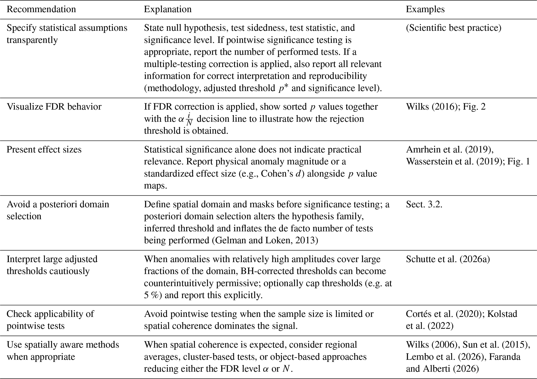
The previous sections demonstrate that statistical significance assessment of geospatial data when conducting large number of tests is complex, and that controlling for the global error rate comes with its own pitfalls. In particular, the widely-used BH correction can invite inappropriate local interpretations when results are visualized on maps, leading to strongly domain-dependent conclusions. Table 2 summarizes a set of practical recommendations aimed at improving robustness, interpretability, and transparency in geoscientific significance assessment. We briefly elaborate on these points below.
A first requirement is transparent reporting of all statistical assumptions. Studies should clearly specify the null hypothesis, test sidedness, test statistic, and significance level. Furthermore, if pointwise testing is appropriate, the pointwise significance level and the number of tests performed should be reported. Likewise, one should explicitly state whether multiple-testing correction has been applied and, if so, the resulting adjusted threshold. Visualizing the behavior of the FDR correction procedure, for example through ranked p-value plots as shown in Fig. 2, can substantially improve interpretability and facilitate open discussion of statistical decisions.
A related point concerns what significance actually tells us. A low p value indicates that the observed value of the chosen test statistics supports rejection of the null hypothesis in favor of the specified alternative with low probability of error, but it says nothing about whether the underlying signal is large enough to matter physically. This gap widens with sample size: even physically negligible anomalies may become statistically significant given a large enough sample size (Wasserstein et al., 2019). We therefore recommend reporting effect sizes, such as the physical anomaly magnitude or a standardized measure like Cohen's d (Cohen, 1988), alongside significance maps. In most geoscientific research, showing physical anomalies is already common practice. For example, Fig. 1 already does this by design, with color shading conveying the magnitude of t2m anomalies and horizontal hatching conveying statistical significance.
Equally important is defining the testing domain a priori. Selecting or modifying spatial domains after inspecting results changes the family of hypotheses being tested and can substantially alter the adjusted significance threshold. As demonstrated in Sect. 3.2, such a posteriori choices can result in misleading interpretations and must be avoided.
An additional question is whether pointwise testing is appropriate at all. Geophysical signals may exhibit strong spatial coherence, while sample sizes remain limited. Sometimes, the sample size may even be too low to perform statistical testing with sufficient statistical power, which should be stated clearly when applicable. Furthermore, grid-point testing may overemphasize unnecessary spatial detail to the detriment of statistical power. In many applications, the scientific question concerns the existence of a regional-scale anomaly rather than the significance of individual grid points. When spatial coherence is expected, spatially aware approaches can provide a more consistent alternative to pointwise hypothesis testing. Instead of evaluating each grid point independently, the analysis can be performed on spatially aggregated quantities that better reflect the underlying physical structure of the system. Examples include regional averages, spatial clusters, or object-based approaches, in which coherent features such as circulation structures or contiguous regions exceeding a predefined threshold are identified and treated as statistical units in the analysis. Again, such choices should be made a priori based on the research question prompting the statistical analysis and should not follow preliminary significance testing or data inspection. By reducing the dimensionality of the problem, these approaches decrease the number of independent tests and align statistical inference more closely with physically meaningful structures.
The regional mean temperature analysis presented above provides a simple illustration. Considering only land points, the regional mean 60 d t2m anomaly over northern Europe is negative and can be assessed using a single hypothesis test (p=0.045 obtained from a one-sided, one-sample Student's t test for an area-weighted mean anomaly of −0.99 K). In this case, inference focuses directly on the question of whether a coherent regional response exists, rather than on hundreds of individual grid-point tests whose outcomes are strongly correlated.
Another practical aspect concerns the choice of the FDR level itself. In most applications, the FDR level α is selected a priori (e.g. α=0.1 following Wilks, 2016) and treated as independent of the data structure. However, the behavior of the BH correction depends not only on α, but also on the p values. One straightforward option to reduce the BH-corrected threshold is simply to choose a smaller fixed α (e.g., α=0.05 instead of 0.1). Authors may also consider capping the adjusted threshold at a level defined a priori (e.g. 5 %), stating this choice explicitly. Since applying the BH correction with the suggested α=0.1 can yield adjusted p value thresholds larger than the conventional local 5 % level (see example in Sect. 3.2), setting such an upper limit may reduce the risk of overconfident interpretations of statistical significance. Alternatively, α could be adjusted dynamically based on properties of the tested field, such as the fraction of nominally significant tests or the ratio between domain size and spatial autocorrelation length scale. Adaptive refinements of this kind have been discussed in the wider FDR literature (Benjamini and Yekutieli, 2001; Storey, 2002; Benjamini et al., 2006; Mrkvička and Myllymäki, 2023).
One may also consider opting for other approaches than the BH correction, for instance by addressing the Family-Wise Error Rate (FWER) instead of the FDR. However, FWER-controlling methods derived under an independence assumption tend to become overly conservative under positive spatial correlation (Livezey and Chen, 1983). One can account for spatially correlated signals, for example, by modifying the Walker criterion by replacing the total number of tests N by an effective number of independent tests (Wilks, 2006; Walker, 1914):
Here, Neff<N represents the reduced, effective number of degrees of freedom implied by spatial dependence among grid points. There exist different ways to estimate Neff, e.g., from the spatial autocorrelation structure, or from other definitions of spatial objects or clusters (Bretherton et al., 1999; Griffith, 2013; Dong et al., 2025; Faranda and Alberti, 2026). Framed in this way, Eq. (5) can be interpreted as a pragmatic compromise between fully pointwise inference and purely regional testing.
However, estimating Neff reliably remains challenging. Spatial correlations are typically non-stationary and anisotropic, and their structure varies across variables, regions, and temporal scales. As noted by Wilks (2016), these difficulties limit the robustness of methods that rely on a single global estimate of independence. In this sense, both adapting the FDR level and estimating Neff can be viewed as attempts to reconcile multiple-testing control with the effective dimensionality imposed by spatial dependence.
The peer-reviewed geosciences literature routinely presents statistical significance based on pointwise testing on spatial maps. Multiple-testing correction is essential for any inference drawn from such analyses. Yet, such correction should be applied with care. In this work, we have highlighted a specific caveat of the widely adopted Benjamini-Hochberg (BH) false discovery rate (FDR) correction (Benjamini and Hochberg, 1995; Wilks, 2016). When a large fraction of grid points exhibit strong anomalies, the BH correction can yield a relatively permissive corrected significance threshold. This behavior is expected from the formulation of the BH correction and from the common choice of using an FDR level α higher than the pointwise significance level. It can however lead to overconfident conclusions if statistical significance is interpreted pointwise. This becomes an issue specifically when many studies implicitly or explicitly interpret FDR correction as automatically leading to stricter thresholds.
This permissiveness does not imply that FDR correction procedures are inherently flawed. Rather, it reflects a mismatch between the aim of the BH correction method and the interpretation of statistical significance that is typically given when testing spatially distributed data. The FDR-adjusted significance threshold is designed to control the global error rate, not false discovery at single grid points. Because the BH-adjusted threshold depends on the global rank distribution of p values, it is sensitive to spatial coherence, domain definition, and the proportion of affected grid points. As a result, statistical conclusions derived from maps can change in ways that appear counterintuitive when the tested spatial domain is modified, even if the underlying physical signal remains unchanged. This becomes an issue when analysis domains are chosen a posteriori following exploratory analyses, or when FDR-corrected significance is interpreted as showing locally significant grid points.
We have proposed a set of practical recommendations to improve the robustness and transparency of statistical assessments in geospatial analyses. These include clearly reporting the applied correction method along with all relevant information, cautious interpretation of adjusted thresholds, and considering spatially aware alternatives when appropriate. Such considerations are crucial to ensure reproducibility, comparability and interpretability across studies.
Ultimately, significance assessment in geospatial data involves a trade-off between interpretability and statistical rigor. Pointwise inference provides intuitive spatial detail but risks overstating confidence, whereas spatially aggregated approaches offer stronger error control at the expense of spatial specificity. Developing methods that balance these competing goals while remaining computationally efficient and interpretable remains an important direction for future research.
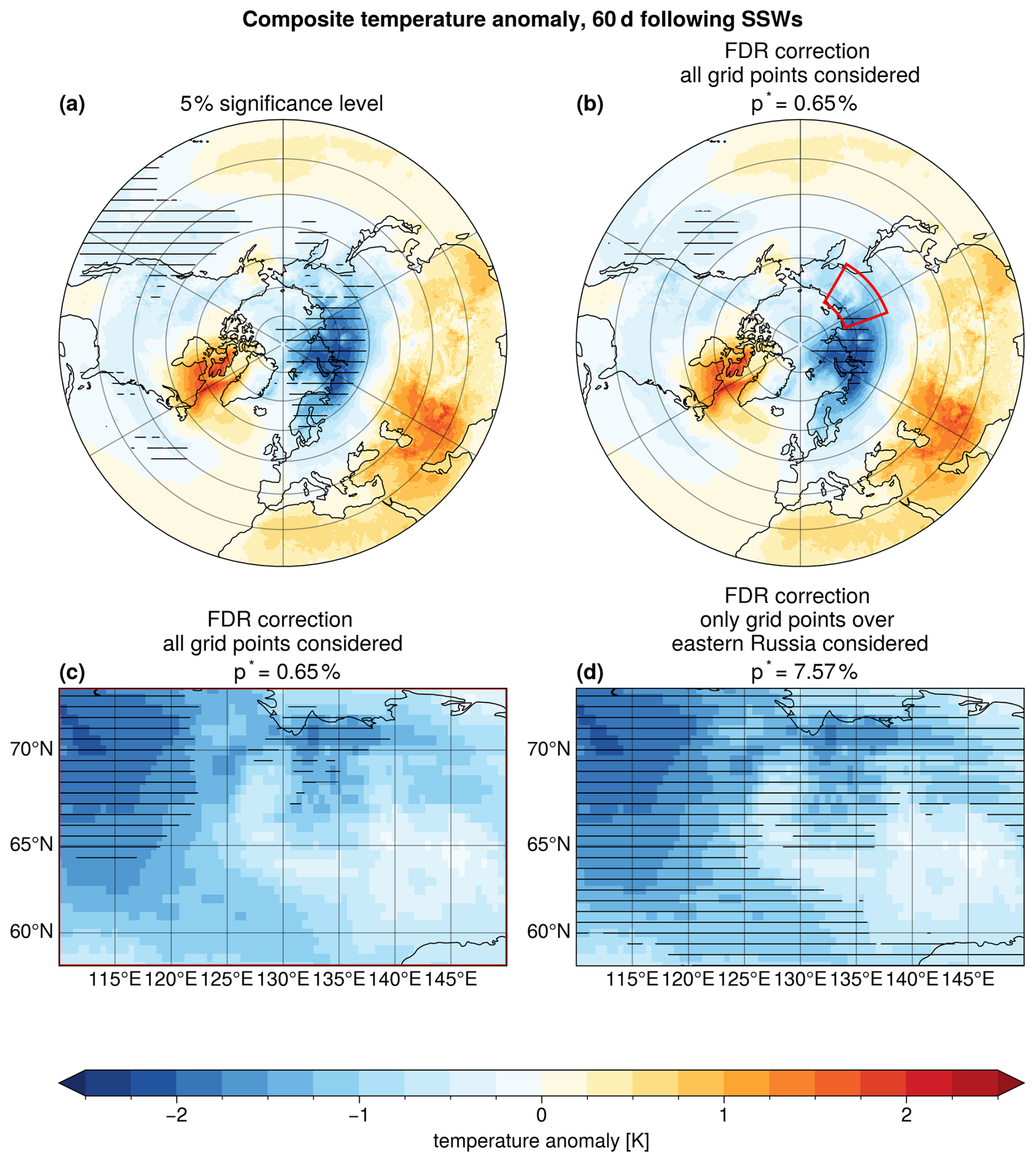
Figure A1As Fig. 1 but for a domain across eastern Russia ranging between 110–150° E, and 58–73° N.
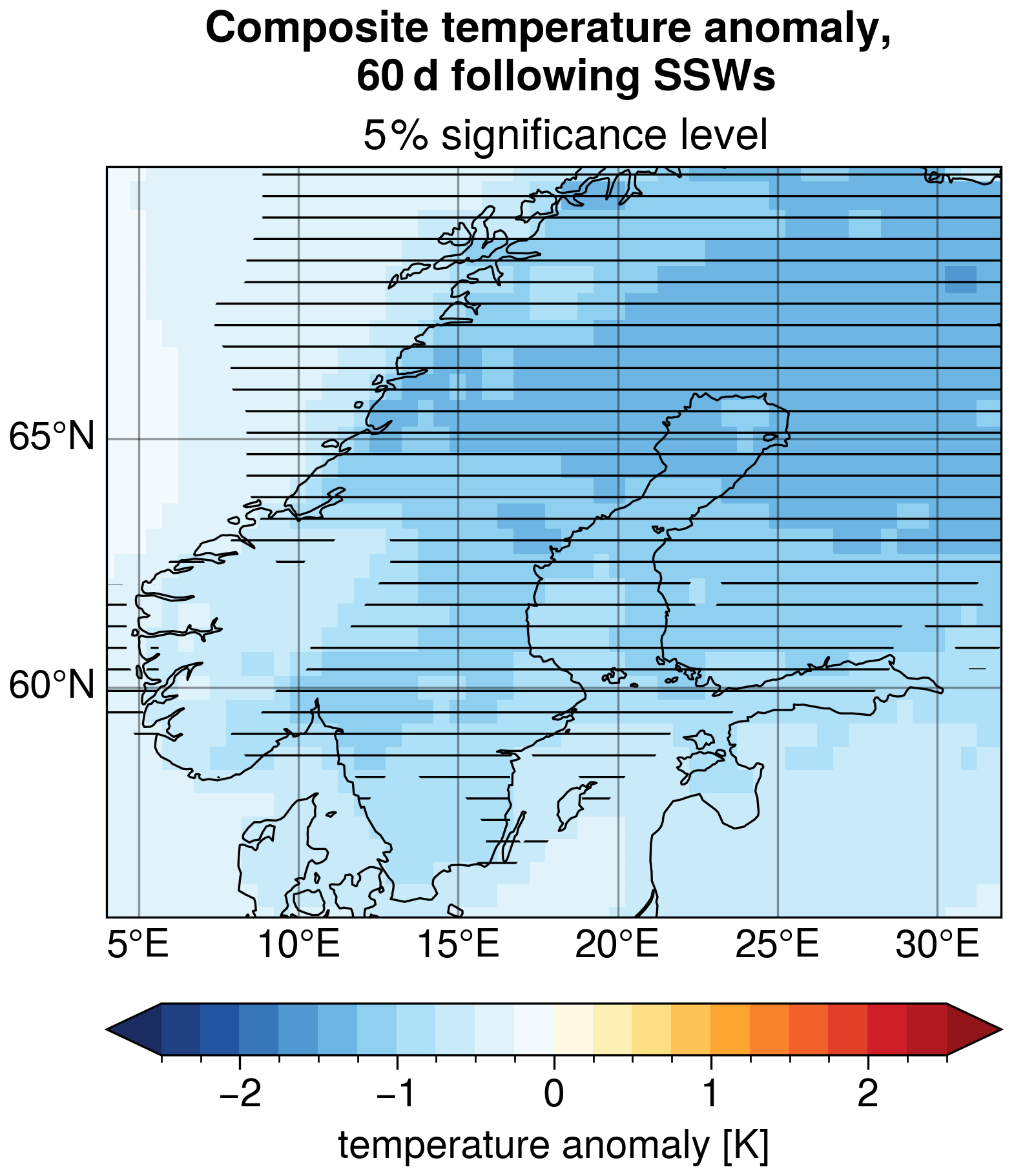
Figure A2Composites of 2 m air temperature anomalies averaged over 60 d following SSWs. Horizontal hatching indicates statistical significance of cold anomalies with respect to a local 5 % significance level, obtained with a one-sided Student's t test.

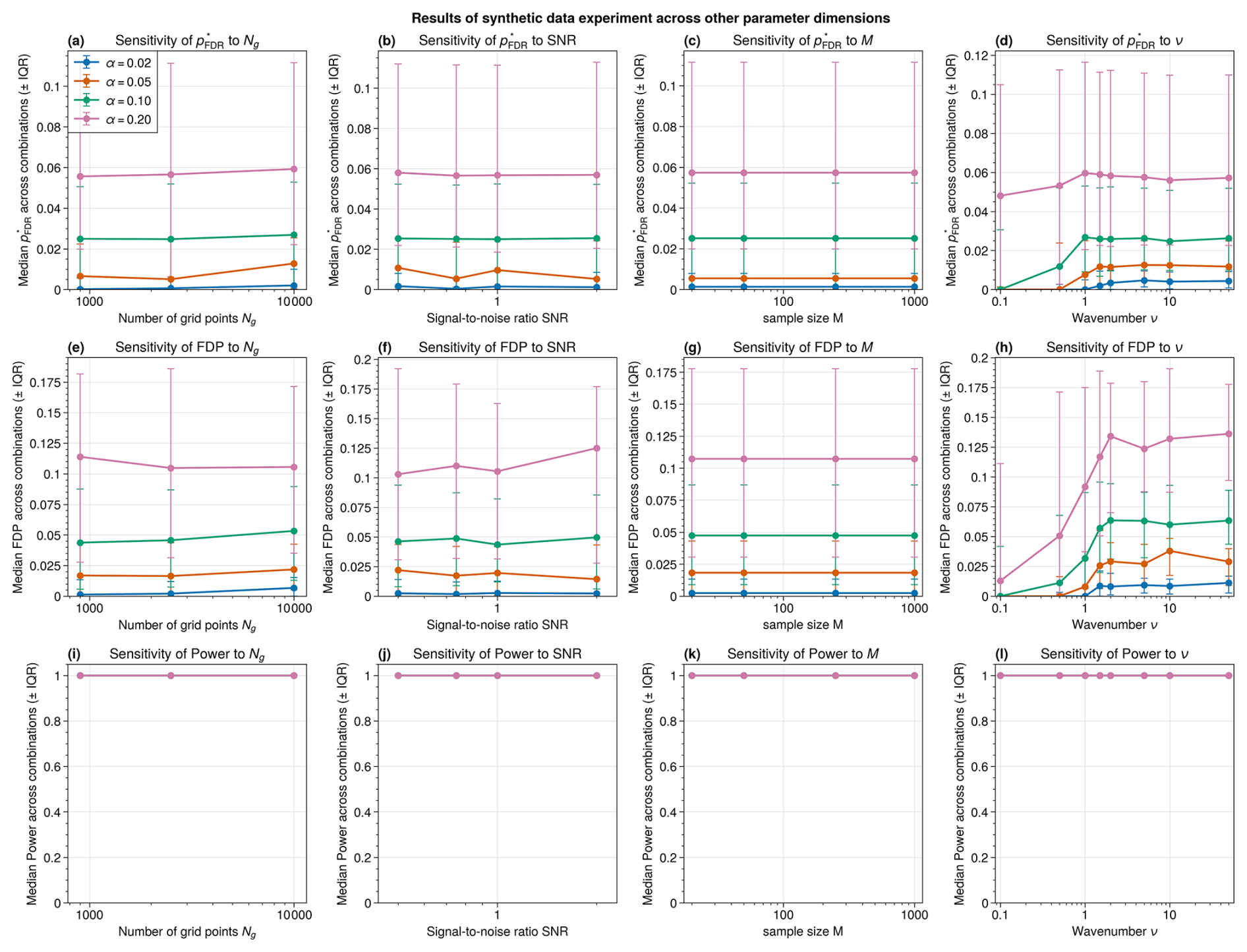
Figure A4Sensitivity of the BH-corrected threshold p* (a–d), realized false discovery proportion FDP (e–h), and power (i–l) to domain size Ng (a, e, i), signal-to-noise ratio SNR (b, f, j), sample size (number of simulated fields per grid point; c, g, k), and noise wavenumber ν (d, h, l). In each panel, markers show the median and error bars the interquartile range across all remaining parameter combinations. Colors indicate the choice of FDR level α as in Fig. 3, given in the legend in panel (a). In the bottom row, the median power across all parameter combinations is shown as a single purple line, as all choices of α yield near-identical power close to unity.
ERA5 data is freely available from https://doi.org/10.24381/cds.bd0915c6 (Hersbach et al., 2025). The code to create the figures and for the numerical experiment is available from https://doi.org/10.5281/zenodo.20280930 (Schutte et al., 2026b).
MKS: Conceptualization, Methodology, Formal analysis, Investigation, Data Curation, Writing – Original Draft, Writing – Review & Editing, Software, Visualization. LO: Conceptualization, Methodology, Investigation, Writing – Original Draft, Writing – Review & Editing, Visualization. FMEP: Conceptualization, Methodology, Investigation, Writing – Review & Editing, Software, Visualization. GM: Conceptualization, Methodology, Writing – Review & Editing, Visualization, Supervision, Funding acquisition.
The contact author has declared that none of the authors has any competing interests.
Publisher's note: Copernicus Publications remains neutral with regard to jurisdictional claims made in the text, published maps, institutional affiliations, or any other geographical representation in this paper. The authors bear the ultimate responsibility for providing appropriate place names. Views expressed in the text are those of the authors and do not necessarily reflect the views of the publisher.
We would like to thank Daniel Stephen Wilks, Davide Faranda, and Antonio Segalini for their helpful feedback on the manuscript. During the preparation of this work the authors used ChatGPT and Claude in order to improve the readability and language of the manuscript. After using this tool/service, the authors reviewed and edited the content as needed and take full responsibility for the content of the published article. The data handling was enabled by resources provided by the National Academic Infrastructure for Supercomputing in Sweden (NAISS), partially funded by the Swedish Research Council Vetenskapsrådet through grant agreement no. 2022-06725.
MS, LO, and GM acknowledge funding from the European Research Council (ERC) under the European Union's Horizon 2020 research and innovation program (grant agreement no. 948309, CENÆ project) and Horizon Europe research and innovation program (grant agreement no. 101231771, DYCLEX project).
The publication of this article was funded by the Swedish Research Council, Forte, Formas, and Vinnova.
This paper was edited by Paul Ullrich and reviewed by three anonymous referees.
Alberton, B. A., Nichols, T. E., Gamba, H. R., and Winkler, A. M.: Multiple testing correction over contrasts for brain imaging, NeuroImage, 216, 116 760, https://doi.org/10.1016/j.neuroimage.2020.116760, 2020. a
Amrhein, V., Greenland, S., and McShane, B.: Scientists rise up against statistical significance, Nature, 567, 305–307, https://doi.org/10.1038/d41586-019-00857-9, 2019. a
Baldwin, M. P. and Dunkerton, T. J.: Stratospheric Harbingers of Anomalous Weather Regimes, Science, 294, 581–584, https://doi.org/10.1126/science.1063315, 2001. a
Baldwin, M. P., Ayarzagüena, B., Birner, T., Butchart, N., Butler, A. H., Charlton-Perez, A. J., Domeisen, D. I. V., Garfinkel, C. I., Garny, H., Gerber, E. P., Hegglin, M. I., Langematz, U., and Pedatella, N. M.: Sudden Stratospheric Warmings, Rev. Geophys., 59, e2020RG000708, https://doi.org/10.1029/2020RG000708, 2021. a
Benjamini, Y. and Hochberg, Y.: Controlling the false discovery rate: a practical and powerful approach to multiple testing, J. Roy. Stat. Soc. B, 57, 289–300, https://doi.org/10.1111/j.2517-6161.1995.tb02031.x, 1995. a, b, c, d, e
Benjamini, Y. and Yekutieli, D.: The Control of the False Discovery Rate in Multiple Testing under Dependency, Ann. Stat., 29, 1165–1188, 2001. a, b, c
Benjamini, Y., Krieger, A. M., and Yekutieli, D.: Adaptive Linear Step-up Procedures That Control the False Discovery Rate, Biometrika, 93, 491–507, 2006. a, b
Bretherton, C. S., Widmann, M., Dymnikov, V. P., Wallace, J. M., and Bladé, I.: The Effective Number of Spatial Degrees of Freedom of a Time-Varying Field, J. Clim., 12, 1990 – 2009, https://doi.org/10.1175/1520-0442(1999)012<1990:TENOSD>2.0.CO;2, 1999. a
Butler, A.: Table of major mid-winter SSWs in reanalyses products, NOAA, https://csl.noaa.gov/groups/csl8/sswcompendium/majorevents.html (last access: 6 October 2026), 2025. a
Butler, A. H., Sjoberg, J. P., Seidel, D. J., and Rosenlof, K. H.: A sudden stratospheric warming compendium, Earth Syst. Sci. Data, 9, 63–76, https://doi.org/10.5194/essd-9-63-2017, 2017. a, b, c, d
Charlton, A. J. and Polvani, L. M.: A New Look at Stratospheric Sudden Warmings. Part I: Climatology and Modeling Benchmarks, J. Climate, 20, 449–469, https://doi.org/10.1175/JCLI3996.1, 2007. a
Cohen, J.: Statistical Power Analysis for the Behavioral Sciences, 2nd Edn., Routledge, New York, https://doi.org/10.4324/9780203771587, 1988. a
Cortés, J., Mahecha, M., Reichstein, M., and Brenning, A.: Accounting for multiple testing in the analysis of spatio-temporal environmental data, Environ. Ecol. Stat., 27, 293–318, https://doi.org/10.1007/s10651-020-00446-4, 2020. a, b
Deser, C., Phillips, A., Bourdette, V., and Teng, H.: Uncertainty in climate change projections: the role of internal variability, Clim. Dynam., 38, 527–546, https://doi.org/10.1007/s00382-010-0977-x, 2012. a
Dong, B., Ullrich, P., Lee, J., Gleckler, P., Chang, K., and O'Brien, T. A.: A new metrics framework for quantifying and intercomparing atmospheric rivers in observations, reanalyses, and climate models, Geosci. Model Dev., 18, 961–976, https://doi.org/10.5194/gmd-18-961-2025, 2025. a
Eade, R., Smith, D., Scaife, A., Wallace, E., Dunstone, N., Hermanson, L., and Robinson, N.: Do seasonal-to-decadal climate predictions underestimate the predictability of the real world?, Geophys. Res. Lett., 41, 5620–5628, https://doi.org/10.1002/2014GL061146, 2014. a
Faranda, D. and Alberti, T.: Investigating the Role of Climate Change in the 3 May 2025 Western Europe Hailstorm Using Atmospheric Analogs, Atmos. Sci. Lett., 27, e70016, https://doi.org/10.1002/asl2.70016, 2026. a, b
Gelman, A. and Loken, E.: The garden of forking paths: Why multiple comparisons can be a problem, even when there is no “fishing expedition” or https://sites.stat.columbia.edu/gelman/research/unpublished/p_hacking.pdf (last access: 8 November 2026), Department of Statistics, Columbia University, unpublished manuscript, 2013. a
Griffith, D. A.: Establishing Qualitative Geographic Sample Size in the Presence of Spatial Autocorrelation, Ann. Assoc. Am. Geogr., 103, 1107–1122, https://doi.org/10.1080/00045608.2013.776884, 2013. a
Hersbach, H., Bell, B., Berrisford, P., Hirahara, S., Horányi, A., Muñoz-Sabater, J., Nicolas, J., Peubey, C., Radu, R., Schepers, D., Simmons, A., Soci, C., Abdalla, S., Abellan, X., Balsamo, G., Bechtold, P., Biavati, G., Bidlot, J., Bonavita, M., De Chiara, G., Dahlgren, P., Dee, D., Diamantakis, M., Dragani, R., Flemming, J., Forbes, R., Fuentes, M., Geer, A., Haimberger, L., Healy, S., Hogan, R. J., Hólm, E., Janisková, M., Keeley, S., Laloyaux, P., Lopez, P., Lupu, C., Radnoti, G., de Rosnay, P., Rozum, I., Vamborg, F., Villaume, S., and Thépaut, J.-N.: The ERA5 global reanalysis, Q. J. Roy. Meteorol. Soc., 146, 1999–2049, https://doi.org/10.1002/qj.3803, 2020. a
Hersbach, H., Bell, B., Berrisford, P., Biavati, G., Horányi, A., Muñoz Sabater, J., Nicolas, J., Peubey, C., Radu, R., Rozum, I., Schepers, D., Simmons, A., Soci, C., Dee, D., and Thépaut, J.-N.: ERA5 hourly data on pressure levels from 1940 to present, Copernicus Climate Change Service (C3S) Climate Data Store (CDS) [data set], https://doi.org/10.24381/cds.bd0915c6, 2025. a
Jeuring, J., Samuelsen, E. M., Lamers, M., Müller, M., Åge Hjøllo, B., Bertino, L., and Hagen, B.: Map-Based Ensemble Forecasts for Maritime Operations: An Interactive Usability Assessment with Decision Scenarios, Weather Clim. Soc., 16, 235–256, https://doi.org/10.1175/WCAS-D-23-0076.1, 2024. a
Katz, R. W.: Sir Gilbert Walker and a Connection between El Niño and Statistics, Stat. Sci., 17, https://doi.org/10.1214/ss/1023799000, 2002. a
Katz, R. W. and Brown, B. G.: The problem of multiplicity in research on teleconnections, Int. J. Climatol., 11, 505–513, https://doi.org/10.1002/joc.3370110504, 1991. a
Kelleher, M. E. and Mahajan, S.: Enhanced climate reproducibility testing with false discovery rate correction, Earth Syst. Dynam., 17, 23–39, https://doi.org/10.5194/esd-17-23-2026, 2026. a
King, A. D., Butler, A. H., Jucker, M., Earl, N. O., and Rudeva, I.: Observed relationships between sudden stratospheric warmings and European climate extremes, J. Geophys. Res.-Atmos., 124, 13943–13961, https://doi.org/10.1029/2019JD030480, 2019. a
Kolstad, E. W., Breiteig, T., and Scaife, A. A.: The association between stratospheric weak polar vortex events and cold air outbreaks in the Northern Hemisphere, Q. J. Roy. Meteorol. Soc., 136, 886–893, https://doi.org/10.1002/qj.620, 2010. a, b, c
Kolstad, E. W., Lee, S. H., Butler, A. H., Domeisen, D. I., and Wulff, C. O.: Diverse surface signatures of stratospheric polar vortex anomalies, J. Geophys. Res.-Atmos., 127, e2022JD037422, https://doi.org/10.1029/2022JD037422, 2022. a, b
Lee, S. H., Butler, A. H., and Manney, G. L.: Two major sudden stratospheric warmings during winter 2023/2024, Weather, 80, 45–53, https://doi.org/10.1002/wea.7656, 2025. a
Lembo, V., Messori, G., Faranda, D., Galfi, V. M., Graversen, R. G., and Pons, F. E.: Concurrent heat waves and their linkage to large-scale meridional heat transports through planetary-scale waves, Weather Clim. Dynam., 7, 453–473, https://doi.org/10.5194/wcd-7-453-2026, 2026. a
Livezey, R. E. and Chen, W. Y.: Statistical Field Significance and its Determination by Monte Carlo Techniques, Mon. Weather Rev., 111, 46–59, https://doi.org/10.1175/1520-0493(1983)111<0046:SFSAID>2.0.CO;2, 1983. a, b, c, d
Monnin, E., Kretschmer, M., and Polichtchouk, I.: The role of the timing of sudden stratospheric warmings for precipitation and temperature anomalies in Europe, Int. J. Climatol., 42, 3448–3462, https://doi.org/10.1002/joc.7426, 2022. a
Mrkvička, T. and Myllymäki, M.: False discovery rate envelopes, Stat. Comput., 33, 109, https://doi.org/10.1007/s11222-023-10275-7, 2023. a, b
Noble, W. S.: How does multiple testing correction work?, Nat. Biotechnol., 27, 1135–1137, https://doi.org/10.1038/nbt1209-1135, 2009. a
Oehrlein, J., Polvani, L. M., Sun, L., and Deser, C.: How well do we know the surface impact of sudden stratospheric warmings?, Geophys. Res. Lett., 48, e2021GL095 493, https://doi.org/10.1029/2021GL095493, 2021. a, b
Pappenberger, F., Cloke, H. L., and Baugh, C. A.: Cartograms for use in forecasting weather-driven natural hazards, Cartogr. J., 56, 134–145, https://doi.org/10.1080/00087041.2018.1534358, 2019. a
Schutte, M. K., Olivetti, L., Krouma, M., and Messori, G.: Stratospheric and tropospheric contributions to North American cold temperatures and subsequent North Atlantic jet stream anomalies, Weather Clim. Ext., 52, 100901, https://doi.org/10.1016/j.wace.2026.100901, 2026a. a
Schutte, M. K., Olivetti, L., Pons, F. M. E., and Messori, G.: Code and data for “The Stippled Gridpoints are Statistically Significant: (Mis)uses of False Discovery Rate Correction for Geospatial Data”, Zenodo [code and data set], https://doi.org/10.5281/zenodo.20280930, 2026b. a
Seneviratne, S., Zhang, X., Adnan, M., Badi, W., Dereczynski, C., A. Di Luca, S. G., Iskandar, I., Kossin, J., Lewis, S., Otto, F., Pinto, I., Satoh, M., Vicente-Serrano, S., Wehner, M., and Zhou, B.: Weather and Climate Extreme Events in a Changing Climate, in: Climate Change 2021: The Physical Science Basis. Contribution of Working Group I to the Sixth Assessment Report of the Intergovernmental Panel on Climate Change, edited by: Masson-Delmotte, V., Zhai, P., Pirani, A., Connors, S. L., Péan, C., Berger, S., Caud, N., Chen, Y., Goldfarb, L., Gomis, M. I., Huang, M., Leitzell, K., Lonnoy, E., Matthews, J. B. R., Maycock, T. K., Waterfield, T., Yelekçi, O., Yu, R., and Zhou, B., Cambridge University Press, 1513–1766, https://doi.org/10.1017/9781009157896.013, 2021. a
Storey, J. D.: A Direct Approach to False Discovery Rates, J. Roy. Stat. Soc. B, 64, 479–498, https://doi.org/10.1111/1467-9868.00346, 2002. a, b
Sun, W., Reich, B. J., Tony Cai, T., Guindani, M., and Schwartzman, A.: False discovery control in large-scale spatial multiple testing, J. Roy. Stat. Soc. B, 77, 59–83, https://doi.org/10.1111/rssb.12064, 2015. a
Taggart, R. J. and Wilke, D. J.: Warnings based on risk matrices: a coherent framework with consistent evaluation, Nat. Hazards Earth Syst. Sci., 25, 2657–2677, https://doi.org/10.5194/nhess-25-2657-2025, 2025. a
von Storch, H. and Zwiers, F. W.: Statistical Analysis in Climate Research, Cambridge University Press, Cambridge, https://doi.org/10.1017/CBO9780511612336, 1999. a
Walker, G. T.: Correlation in seasonal variations of weather, III: On the criterion for the reality of relationships or periodicities, Memoirs of the India Meteorological Department, 21, 13–15, 1914. a, b, c
Wasserstein, R. L., Schirm, A. L., and Lazar, N. A.: Moving to a world beyond “p<0.05”, Am. Stat., 73, 1–19, https://doi.org/10.1080/00031305.2019.1583913, 2019. a, b
Wilks, D. S.: On “Field Significance” and the False Discovery Rate, J. Appl. Meteorol. Clim., 45, 1181–1189, https://doi.org/10.1175/JAM2404.1, 2006. a, b, c
Wilks, D. S.: Statistical Methods in the Atmospheric Sciences, in: vol. 100 of International Geophysics, 3rd Edn.,Academic Press, ISBN 978-0-12-385022-5, 2011. a
Wilks, D. S.: “The Stippling Shows Statistically Significant Grid Points”: How Research Results are Routinely Overstated and Overinterpreted, and What to Do about It, B. Am. Meteorol. Soc., 97, 2263–2273, https://doi.org/10.1175/BAMS-D-15-00267.1, 2016. a, b, c, d, e, f, g, h, i, j, k, l, m, n, o, p
- Abstract
- Introduction
- The false discovery rate
- Example of assessing statistical significance with meteorological data
- The domain dependence of BH correction
- Numerical experiment
- Some practical recommendations
- Conclusions
- Appendix A: Additional figures
- Code and data availability
- Author contributions
- Competing interests
- Disclaimer
- Acknowledgements
- Financial support
- Review statement
- References
- Abstract
- Introduction
- The false discovery rate
- Example of assessing statistical significance with meteorological data
- The domain dependence of BH correction
- Numerical experiment
- Some practical recommendations
- Conclusions
- Appendix A: Additional figures
- Code and data availability
- Author contributions
- Competing interests
- Disclaimer
- Acknowledgements
- Financial support
- Review statement
- References