A simple weather generator that converts statistical information from downscaled global climate models to sequences of daily precipitation and temperature

A simple weather generator is presented that is designed to provide a link between downscaled precipitation or temperature statistics on the one hand, and impact models on the other. It generates time series of daily data that may be used as input for e.g. a hydrological model. It has a simple design which is described in this paper together with results from an evaluation against three rain gauge observations from Norway, Ghana and Romania respectively. It has also been tested for daily precipitation and temperatures from a number of sites representing different local climates in Ghana and Norway, and the results from these evaluations indicate that it reproduces the salient character in terms of the daily data and the observed climatology in different climatological settings. The simple design for precipitation, however, underestimate the duration of dry and wet spells for some sites to some degree. An assessment of the performance of daily temperature simulations from complimentary temperature-based weather generator for test sites in Ghana and Norway suggests that its output follows a similar statistical distribution as the original observations, however, there was some deviations particularly for the lowest temperatures. These two weather generators for daily precipitation and temperature respectively are part of the open-access R-package “esd” (version 1.11.30 or higher).

1 Introduction

Global climate models (GCMs) are our most important tool for simulating future climatic conditions, such as World Climate Research Programme's (WCRP) Coupled Model Intercomparison Project (CMIP) phase 5 and 6 (Meehl et al., 2014; Eyring et al., 2016; IPCC, 2021). Numerical experiments have revealed that a single GCM starting with different initial conditions can produce different regional outlooks due to inherent chaotic (non-deterministic) decadal variability (Deser et al., 2012, 2020), and an important consideration for robust information about a future climate is to involve large GCM ensembles. Furthermore, the GCMs are only designed to reproduce large-scale processes, phenomena and conditions with skill, and are known to have a minimum skilful scale (Takayabu et al., 2015). However, detailed small-scale information is needed for inferring local consequences of climate change, such as its impact on nature or for a risk analysis to inform climate change adaptation (IPCC, 2023). For instance, hydrological models often require sequences of hourly or daily local rainfall and temperature, and are often calibrated with in-situ historical rain gauge measurements (Engeland and Alfredsen, 2020). When such models are used for assessing future consequences of a continued global warming, they need new input data which both represent the same type of conditions as in the past but also account for a shift in the weather statistics associated with climate change (Fowler et al., 2007; Semenov, 2007).

Skilfully reproduced large-scale information distilled from GCM simulations can be combined with information about how local details depend on the large scales in what is known as downscaling, for which there traditionally have been two main approaches (Takayabu et al., 2015; Fowler et al., 2025): (1) dynamical, performed with regional climate models (RCMs), and (2) empirical-statistical downscaling (ESD). Downscaling with RCMs and ESD are based on different assumptions and have different strengths and weaknesses. RCMs use physics-based equations to compute weather information with a higher resolution than GCMs, with model time steps on the order of a few minutes for typically hundreds of variables for each grid cell within a regional domain (Giorgi and Mearns, 1999). This is computationally very expensive, limiting the number of GCM runs that can be downscaled dynamically.

ESD, on the other hand, determines statistical relationships between large-scale structures provided by global models and local climatic conditions, and is typically carried out for one or two variables (Benestad et al., 2008). This makes ESD computationally cheap and enables it to be applied to large multi-model ensembles of GCM simulations (Schuler et al., 2025; Benestad et al., 2025, 2016; Benestad, 2011). It is best suited for downscaling large multi-model ensemble when ESD involves the estimation of statistical parameters describing the shape of mathematical curves (“downscaling climate”), as opposed to estimating each individual data point (“downscaling weather”) (Benestad et al., 2025). Moreover, the wet-day frequency f_w and wet-day mean precipitation μ are two key parameters for 24 h precipitation which are found to change with a global warming (Benestad et al., 2019), and such downscaled statistical information from ESD can only be utilised in subsequent hydrological models if it can be unfolded as sequences of daily precipitation amounts through a conditional weather generator (WG). This implies that in addition to the reproduction of the stochastic character of regional decadal climate variations by global climate models highlighted by Deser et al. (2012, 2020), simulated local annual precipitation or temperature statistics also give room for a range of different random weather outcomes as generated by WGs.

A WG can be described as a “weather dice” that produces random (stochastic) daily data with prescribed statistical properties and structure. There are numerous types of WGs (Wilks, 1992; Wilks and Wilby, 1999; Mezghani and Hingray, 2009; Semenov and Barrow, 1997; Semenov and Brooks, 1999), however, none have in the past been designed specifically to connect ESD, which aims at downscaling the key parameters f_w and μ, to impact models. Furthermore, previous ESD efforts haven't involved estimating such parameters so that they could be adapted to hydrological models that require daily precipitation as input data (Benestad, 2025). In the SPRINGS project (https://www.springsproject.eu/, last access: 11 November 2026) the WG is part of a modelling chain that links the dispersion of waterborne pathogens to climate change, and ultimately outbreak of diarrhoea in Ghana and Romania. In other words, it facilitates a link that passes information from downscaling of GCMs on to hydrological models by generating stochastic daily sequences of rainfall with downscaled statistical properties as input data. The SPRINGS project intends to use the SWAT hydrological model (Gassman et al., 2014), however the WG can also be used to translate rainfall statistics into useful input for the HBV model (Bergström, 1976; Lindström et al., 1997).

Figure 1 shows a schematic of the simple WG for precipitation, which in this case is designed to translate the downscaled key precipitation parameters f_w and μ to appropriate input data for hydrological models that need chronological sequences of daily rainfall from a single site. The WGs for precipitation and temperature are a part of the free and open-source R-package esd (Benestad et al., 2015b) 1.11.30 or later versions, which is available from https://github.com/metno/esd (last access: 11 November 2026). The R-package provides documentation on its usage as well as some examples of use. The WGs are designed with a flexibility in how they can be applied that is controlled by their arguments, and by default they use daily data from Norway provided by the R-package, but it can be replaced with data from any other location. For the use in Ghana with its rainy seasons, for instance, it needs local rain gauge data with a representative climatology.

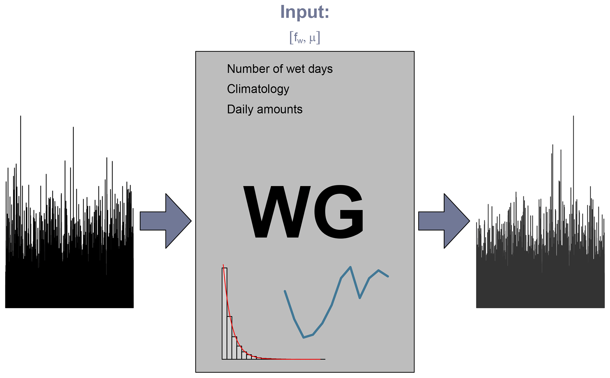
Figure 1 A schematic presentation of the WG which takes a sample station series for training. It can then take f_w and μ as input in order to simulate a random sequence of 24 h precipitation with the same statistical properties. The WG uses a sample rain gauge sequence for determining the climatologies in wet-day frequencies f_w and wet-day mean precipitation μ for a chosen location. In other words, it is designed to reproduce how the number of wet days typically vary throughout the year (rainy seasons) as well as the intensity of the precipitation. If annual f_w and μ are not provided, it will estimate them from the sample data but shuffle the years by scrambling the Fourier Series phases. The histogram in the schematic reflects the mean intensities characterised by μ and the blue curve refers to a climatological profile that can refer to either f_w of μ.

2 Design of the simple weather generator for daily precipitation

One requirement of the WG in a model chain from global climate models to local hydrology is that it must be able to simulate changed rainfall due to changes in the wet-day frequency f_w and wet-day mean precipitation μ. In addition, it must provide a realistic representation of the rainy seasons in the Tropics, and this differs with traditional WGs based on a Markov-chain process, where the probability of a wet day depends on the previous day. Markov-chains are not defined for reproducing rainy seasons unless the probabilities vary with the seasons. Furthermore, the WG was designed to ensure that the number of rainy days and intensities are consistent with prescribed f_w and μ in addition to preserving their climatological properties in both f_w and μ. The mean precipitation is approximately the product of the two $\stackrel{\mathrm{‾}}{x}\approx f_{\mathrm{w}}\mathit{\mu }$ and the total precipitation is the product between the mean and the number of days $\sum x=n\stackrel{\mathrm{‾}}{x}$. Since a cut-off threshold x₀ of 1 mm d⁻¹ has been used to distinguish between “dry” and “wet” days, the equation is only approximate, but for a limit threshold that approaches zero, it is an exact equation as $\overline{x}=\sum x/n=(\sum x/n_{\mathrm{wet}})\cdot (n_{\mathrm{wet}}/n)=\mathit{\mu }{f}_{\mathrm{w}}$. Because of this relationship, the traditional rainfall climatology is also expected to be representative as long as the climatologies for both f_w and μ are realistic.

Simulations with this simple WG involve a process which loops over individual years, and for each year in the loop, it starts with estimating the total number of wet days based on the annual wet-day frequency for the respective year (n_wet=365.25f_w). The following step is then to distribute n_wet wet days over the year based on a climatological profile of f_w, which is used as a representation of the probabilities of a wet day on a given Julian day p_t,wet. To get an annual number of wet days that approximately is the same as n_wet, the entire curve describing the climatological profile is scaled so that the its mean value is equivalent to the annual wet-day frequency. Here p_t,wet is the probability of a wet day for the Julian day $t\in [\mathrm{1},n_y]$ of the respective year, where n_y is 365 d for normal years and 366 days for leap years. A random number generator with a uniform distribution $W_t\in [\mathrm{0},\mathrm{1}]$ is subsequently used to determine whether the individual Julian days are dry or wet according to $\mathrm{wet}\Leftarrow W_t<p_{t,\mathrm{wet}}$. The total number of wet days is then compared with n_wet, and a subsequent process removes or adds random wet days so that the final number matches the expected number n_wet associated with the annual wet-day frequency.

Once all the wet days have been dealt out throughout the year, they are given a daily rainfall amount. The simulation of the 24 h amounts is based on an approximation by the exponential distribution $X\sim \exp (\mathrm{1}/\mathit{\mu })$ and subsequently adjusted by a scaling factor based on its return value ${\mathit{\beta }}^{\prime }=\mathrm{1.256}+\mathrm{0.064}\ln \left(\mathit{\tau }\right)$, where τ is the return interval in terms of years (Benestad et al., 2019). In this expression β^′ is a best-fit coefficient derived from a regression analysis with estimates of return values against the log of its return interval for a large number of available rain gauge measurements world-wide. In other words, the amounts are derived by a random number generator that produce n_wet numbers with an exponential distribution that subsequently are scaled by matching their probabilities according to prescribed distribution with the return interval $p=(\mathrm{365.25}\cdot \mathit{\tau }{)}^{-\mathrm{1}}$, and the end result is pseudo-exponentially distributed. In order to ensure a typical climatological profile in the intensity, both the wet-day mean precipitation μ climatology and the simulated random daily amounts X_t are ranked, and the latter is then sorted with similar ranking. However, a random noise term (a “smudge” factor) is introduced to the ranking of the climatology for each year (different noise term for each year) to avoid an unnaturally sharp peak in the climatology and avoid piling up the greatest precipitation amount on one particular Julian day for all years. The default smudge factor is set to ${\mathit{\sigma }}_{{\mathit{\mu }}_{\mathrm{clim}}}\stackrel{\mathrm{‾}}{{\mathit{\mu }}_{\mathrm{clim}}}/\mathrm{2}$ after trial and error with daily precipitation data from Bjørnholt north of Oslo (as in Fig. 2). This factor can be changed according to site through the argument WG(mu.smudge=), as the default setting may not be appropriate for all locations.

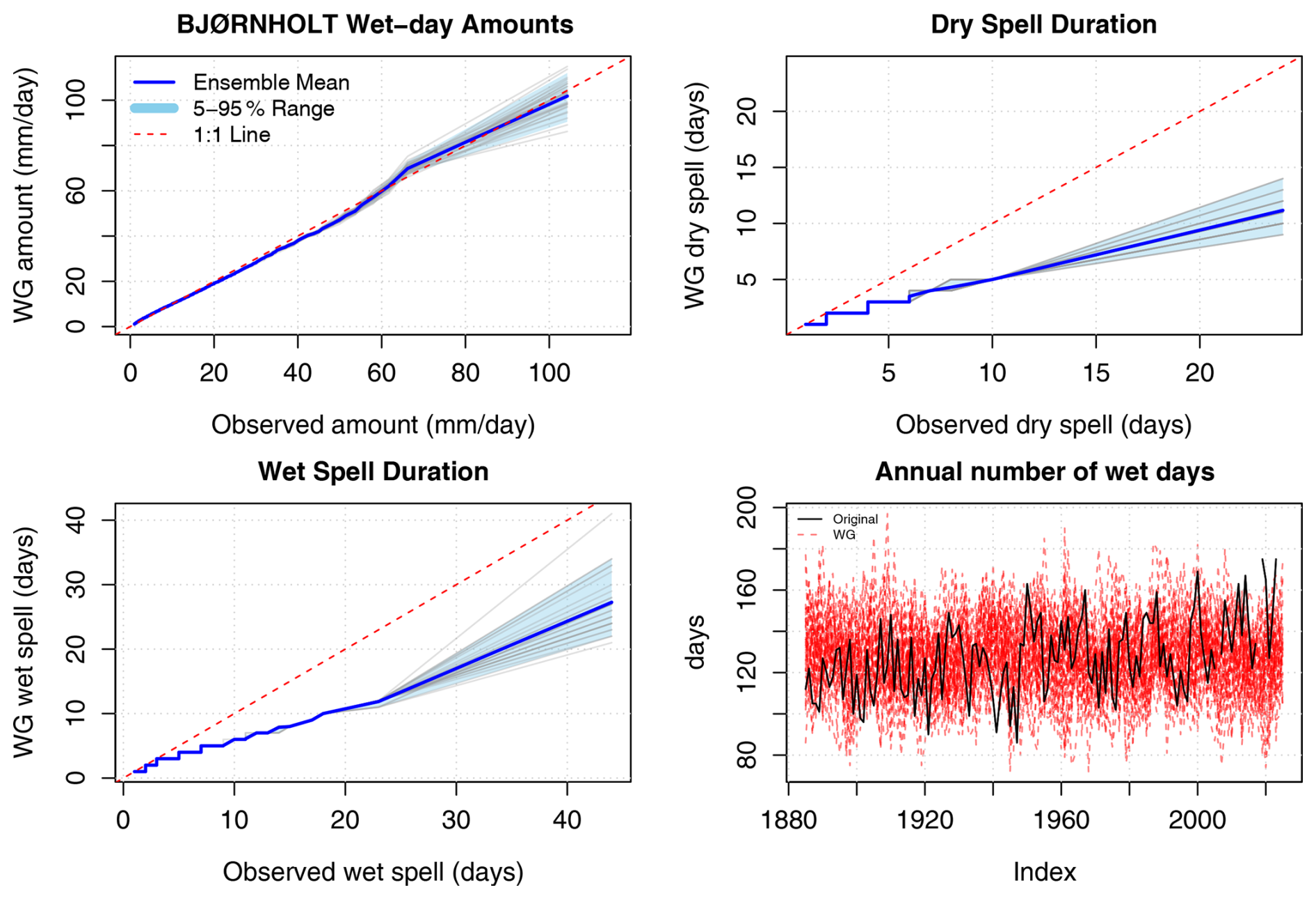
Figure 2 Test results for the WG applied to Bjørnholt rain gauge measurements north of Oslo, Norway. The WG simulations consist of an ensemble with 30 independent runs. Upper left shows a quantile-quantile plot of the observed as opposed to simulated daily rainfall amounts; upper right panel shows a quantile-quantile plot that compares the observed and simulated dry spell durations; and lower left shows a comparison between observed and simulated dry-spell durations; Lower right panel compares the number of annual wet days with original data shown in black and 30 random WG simulations as red dashed line. Data source: Norwegian Meteorological Institute (https://frost.met.no/index.html, last access: 11 November 2026).

Unless prescribed, the annual wet-day frequency f_w and wet-day mean precipitation μ are estimated from the training rain gauge series, but their chronology is scrambled while keeping the temporal structure. The scrambling procedure involves a Fourier transform $F\left(y\right)={\sum }_i{a}_i\cos \left(w_{i}t\right)+b_i\sin \left(w_{i}t\right)$, where the coefficients a_i and b_i determine the spectral power ($a_i^{\mathrm{2}}+b_i^{\mathrm{2}}$) of their respective frequencies, and the scrambling involves changing these coefficients in a conservative way so that the spectral power for each frequency is the same as in the original data. This is equivalent to introducing random phase shifts to all spectral components. If prescribed, on the other hand, the input of the WG may be (1) downscaled annual f_w and μ, or (2) the arguments may be single numbers which it will add to the scrambled annual f_w and μ derived from the training data to mimic a changed climate. Some examples of how the WG can be used are provided in Algorithms A1–A2 in Appendix A.

2.1 Evaluation of the weather generator for daily rainfall

The WG for daily precipitation was tested and evaluated against daily rain gauge data from Norway, Ghana and Romania, and involved a comparison between observed and predicted daily amounts as well as wet/dry spell duration and climatology. Figure 2 shows the test results for Bjørnholt, Oslo, Norway, and a quantile-quantile plot (upper left) shows a good agreement between the daily precipitation amounts from the rain gauge measurements and the output of the WG. There are modest deviations in the upper quantiles beyond 60 mm, but this is also expected due to random sampling fluctuations. The upper right and lower left panels show a comparison between dry-spell and wet-spell durations, and the test indicated that the WG had a tendency to generate too few long wet spells (greater than 5 d) as well as too few long dry spells (greater than 3 d). In this case, the spell durations had not been considered other than being a result of probabilities connected to the f_w climatology, but this aspect can be improved through a subsequent step where single wet days are moved to the nearest cluster of wet days in a way that doesn't strongly change the simulated climatologies. The lower right panel shows a comparison between the annual number of wet days (based on f_w), and the WG did not indicate the same modest trend as the observations since the annual precipitation statistics a had been scrambled through a Fourier transform with random phases.

Figure 3 shows further diagnostics of the WG, and the upper left panel compares the sum of total annual precipitation. The WG produced results which were comparable to the observations in terms of mean level and annual spikes. Furthermore, it reproduced the climatologies in terms of total precipitation (upper right), wet-day frequency (lower left) and wet-day mean precipitation (lower right) reasonably well. Root-mean-square-errors (RMSE) were estimated for the climatology for total precipitation (upper right panel in Fig. 3) for each simulation and were in the range 4.0–6.8 mm for the ensemble runs representing Bjornholt (Table 1) and are relatively small compared to the the monthly totals of 60–140 mm. Furthermore, the RMSE for the climatology of the the wet-day mean precipitation (lower right panel) sand wet-day frequency (lower left panel) were 0.26–0.48 mm d⁻¹ and 0.011–0.016 respectively, which also are modest compared to the climatologies themselves (7–11 mm d⁻¹ for μ and ∼0.4 for f_w respectively). A Kolmogorov-Smirnov test was used to compare the spell duration distributions of the observations made at Bjørnholt and a 30-member ensemble with WG simulations, and the test results were D=0.13 for the dry periods and D=0.20 for wet spells, both with a p-value $<\mathrm{2.2}\times {\mathrm{10}}^{-\mathrm{16}}$. A value of D≈0 would indicate a close match, D≈1 signifies completely distinct statistical properties, and an interpretation of the test results of 0.1–0.2 is therefore a partial match.

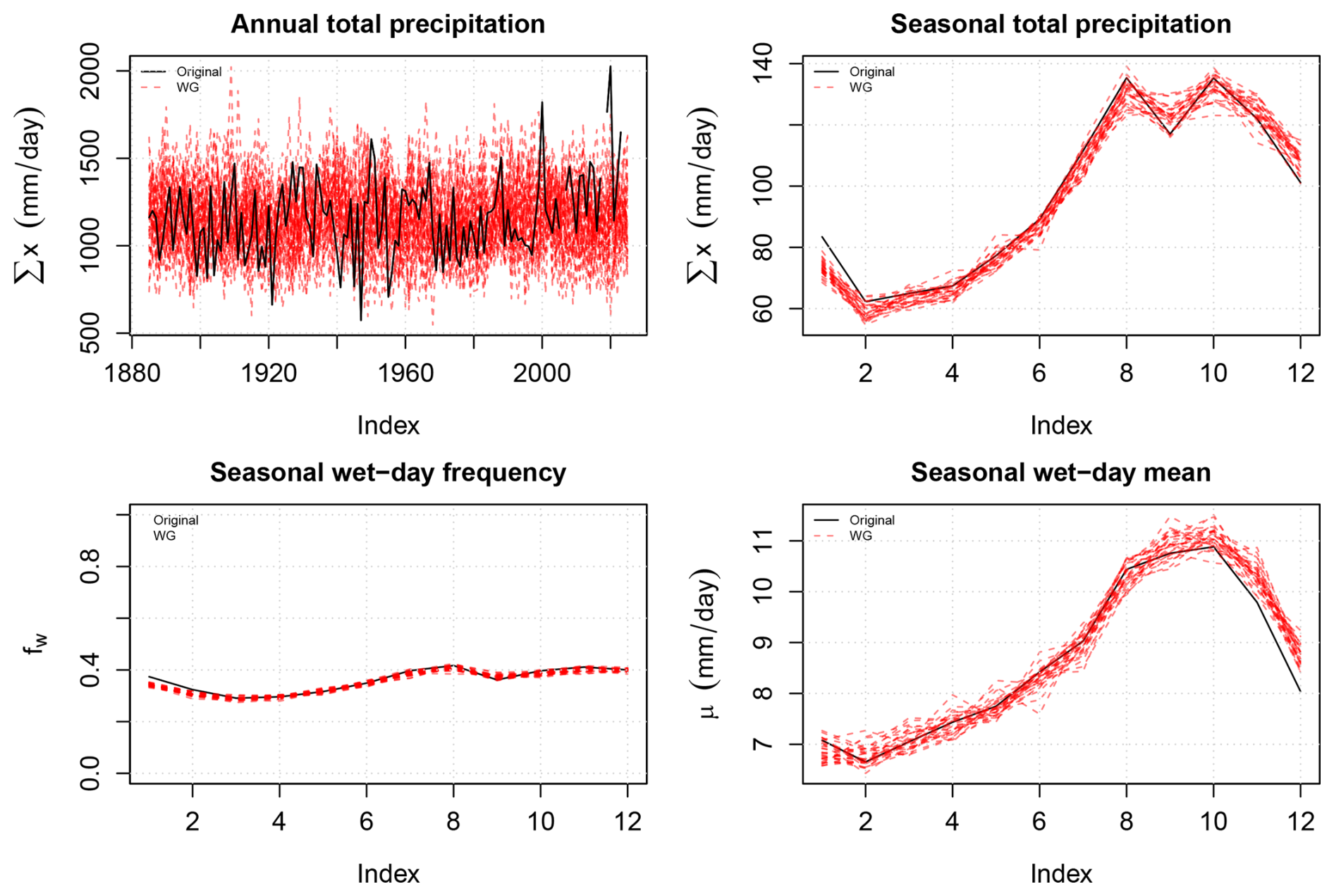
Figure 3 Test results which show a comparison between observed and simulated annual total precipitation (upper left), total rainfall distributed over the year (lower left), the climatology in f_w (upper right) and the climatology in μ (lower right). Data source: Norwegian Meteorological Institute

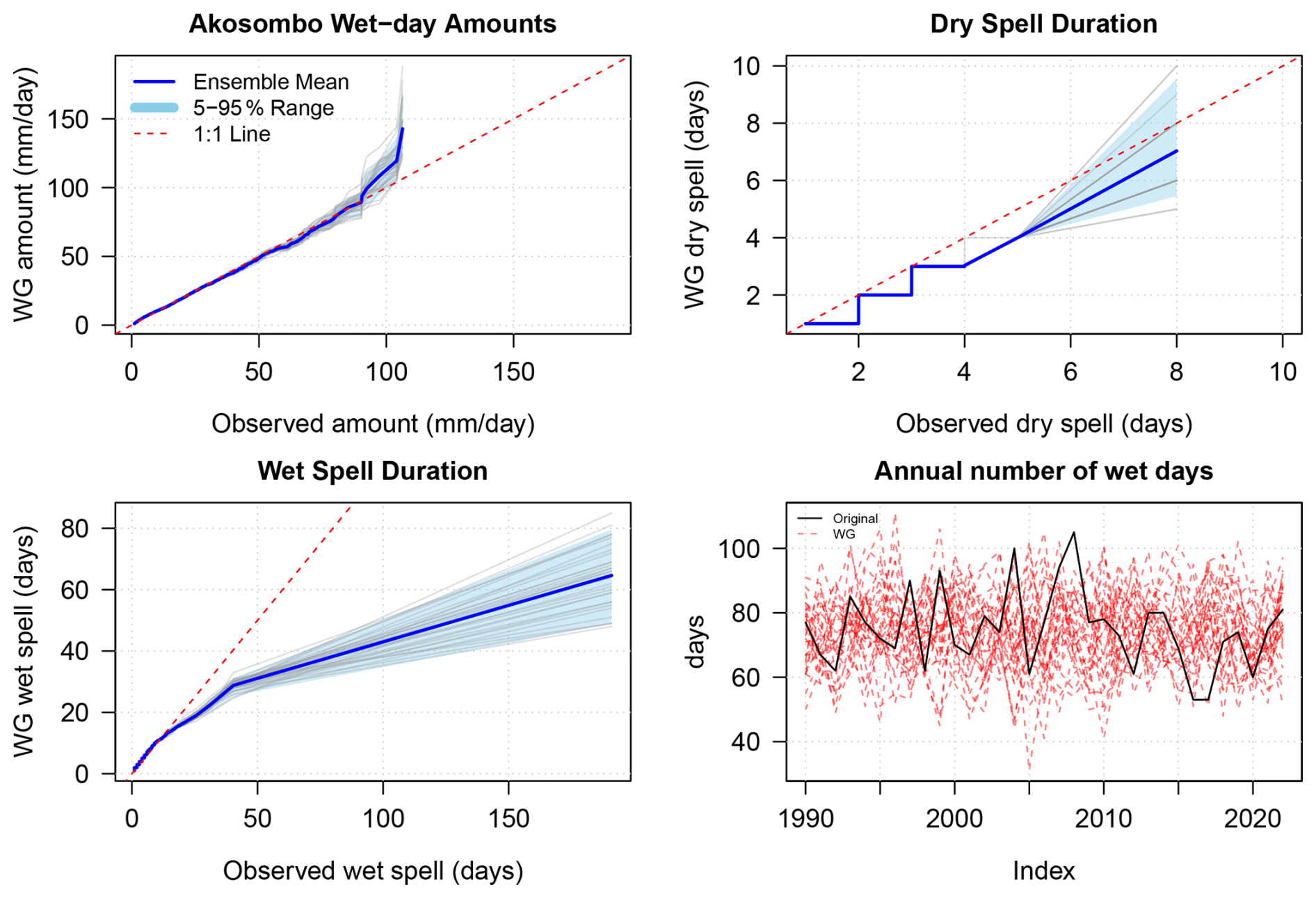
Figure 4 Same as Fig. 1 but for Akosombo in Ghana. The data source is the Ghana Meteorological Agency.

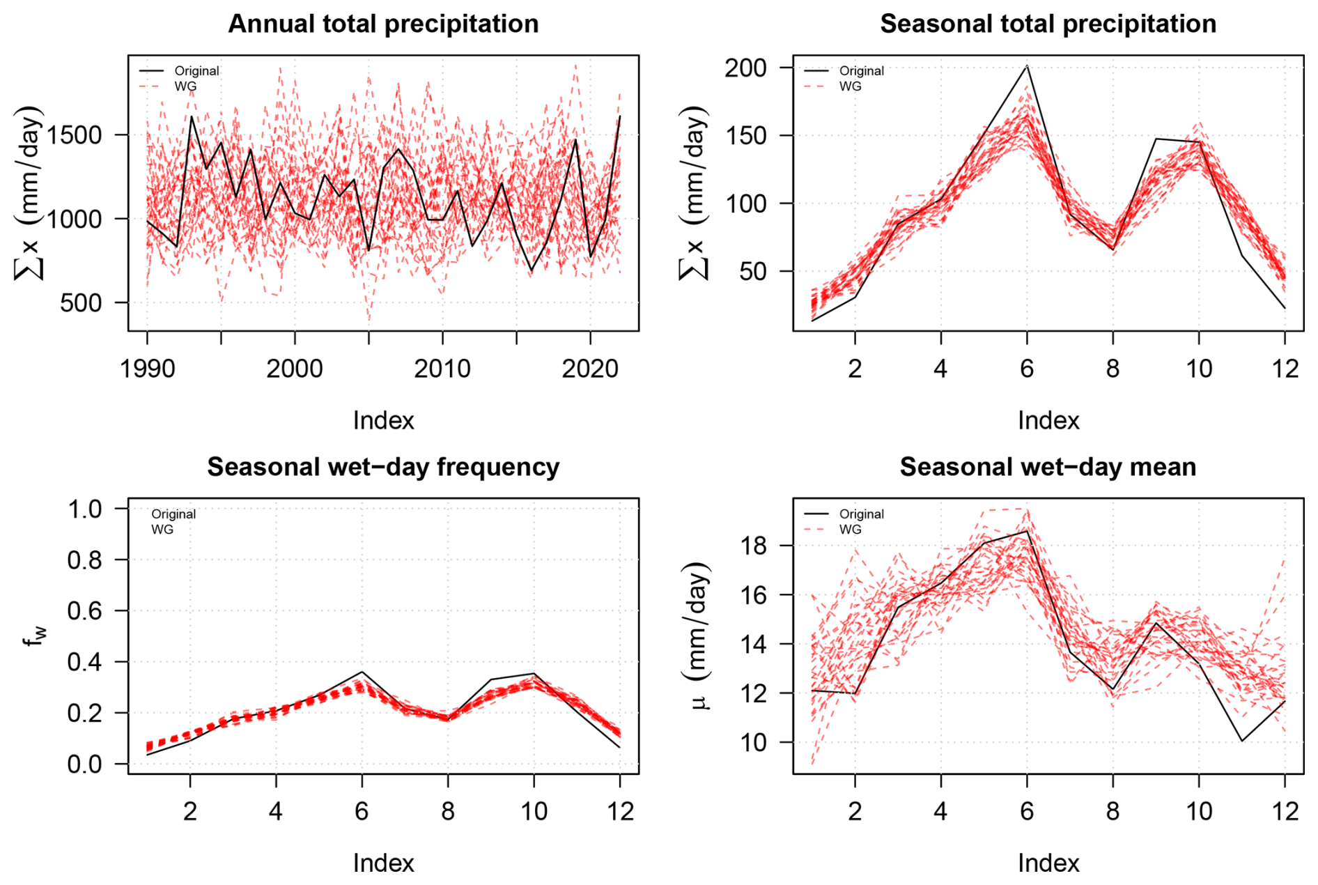
Figure 5 Same as Fig. 2. but for Akosombo in Ghana. The data source is the Ghana Meteorological Agency.

Figures 4–5 show results from a similar evaluation for Akosombo in Ghana which also indicate a reasonable reproduction of the daily data. In this case, the data was provided by Ghana Meteorological Agency and shared within the SPRINGS project, but the rain gauge record from Ghana was much shorter than the Bjørnholt series, only covering the 1990–2025 period. The training of the WG improves with long high-quality data, and some of the discrepancies between observed and modelled results may be due to the limited amount of data. Still, the WG reproduced daily amounts of up to 100 mm that match the quantiles of the observations (upper left panel in Fig. 4). The spell duration statistics was based on a limited sample size, and the WG underestimated durations greater than 30 d in this case (lower left panel in Fig. 4). The WG nevertheless reproduced the main features of the climatologies in the total precipitation, wet-day frequency and wet-day mean precipitation.

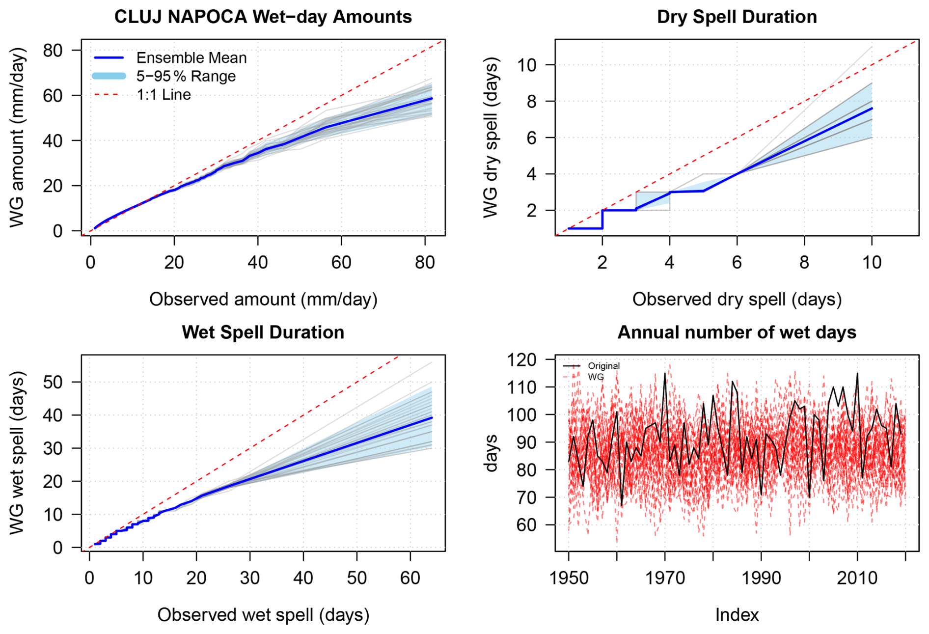
A similar assessment was carried out for daily precipitation from Cluj-Napoca in Romania using rain gauge data from ECA&D (Klein Tank et al., 2002) covering the period 1950–2020, and the results of the evaluation for Romania are presented in Figs. 6–7. In sum, the evaluation of the simple WG for daily precipitation suggested that is gave an approximate description of various aspects of precipitation, but also produced somewhat diverging statistics of dry and wet spell duration. The WG reproduced the observed daily amount up to 20 mm and slightly underestimated greater amounts. It also generated realistic spell durations shorter than 5 d, but underestimated the longer wet and dry episodes. The climatologies were also approximately reproduced for Cluj-Napoca, ensuring realistic seasonality for the precipitation.

Figure 6 Same as Fig. 1 but for Cluj Napoca in Romania. The data source is ECA&D.

Figure 7 Same as Fig. 2. but for Cluj Napoca in Romania. The data source is ECA&D.

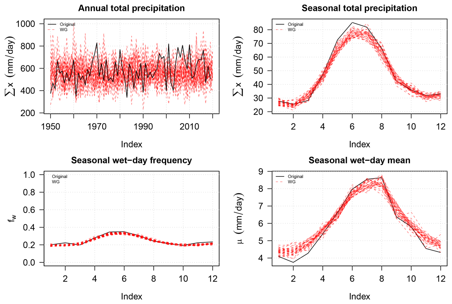
RMSE estimated for the simulated precipitation climatologies for Bjørnholt, Akosombo and Cluj-Napoca are summarised in Table 1 which suggest that the WG reproduced the said climatologies with marginal errors. The WG was also tested against local rainfall from GHCND (Menne et al., 2012; Durre et al., 2010) in Arusha (Tanzania), Naples (Italy), as well as various locations in Norway and spatially aggregated daily rainfall over different sub-basins over the Volta catchment in Ghana based on CHIRPS (Funk et al., 2015) (see the supporting information at https://doi.org/10.6084/m9.figshare.33204858, Benestad, 2026b). The Norwegian rain gauge stations were used in this case because they are open access data from thredds, which makes it easy for others to reproduce the same analyses if they can use R and have the most recent esd-package installed. One point to make is that this WG is easy to use and test with any daily rain gauge station data, and users should also do so for the location of their interest as it only takes a minute or so.

Table 1 Root mmean squared errors (RMSE) estimated for the climatologies of the simulated daily precipitation for Bjørnholt in Norway, Akosombo in Ghana and Cluj-Napoca in Romania.

3 A simple weather generator for daily temperature

A WG simulating temperature has to deal with different considerations than a WG simulating precipitation, as the temperature is a continuous function in time as opposed to the intermittent nature of precipitation. Hence, there is no need to split the days into two categories for temperature, such as “dry” and “wet” days for daily precipitation. Furthermore, daily temperature anomalies (after removing the daily climatology describing the mean seasonal cycle) can be approximated by the normal distribution $T_{\mathrm{2}\mathrm{m}}\sim \mathcal{N}(\mathit{\mu },{\mathit{\sigma }}^{\mathrm{2}})$, and hence the WG for daily temperature uses the mean and standard deviation as two input parameters for determining its nature. Since any time series can be expressed in terms of a sum of a set of harmonics (cosines and sines), we can use a Fourier series as a basis for the temperature-based WGs. The WG for temperature also uses a phase-scrambled Fourier series, but uses it on the daily anomalies in order to preserve time structures such as auto-correlations. Again, the phase-scrambling involves randomising the coefficients a_i and b_i while ensuring that the spectral power expressed in terms of $\sqrt{a_n^{\mathrm{2}}+a_n\mathrm{²}}$ is conserved and matches the original data. Moreover, the WG subtracts the temperature climatology before applying the Fourier Transform and phase scrambling to anomalies, and the scrambled data then provide probability estimates, given its mean value and standard deviation. The scrambled anomalies are subsequently subject to a transform $\mathcal{N}({\mathit{\mu }}_{\mathrm{0}},{\mathit{\sigma }}_{\mathrm{0}}^{\mathrm{2}})\to \mathcal{N}({\mathit{\mu }}_x,{\mathit{\sigma }}_x^{\mathrm{2}})$, where μ_x and σ_x are new mean and standard deviations, and the climatology is subsequently reintroduced to the final transformed anomalies in order to mimic the original temperatures. Some test results for Akosombo in Ghana are shown in Fig. 8 in the shape of a quantile-quantile plot, and the comparison with the original data indicates a reasonably good reproduction of the temperatures except for a bias for temperatures lower than 28 °C. Since the temperature simulations involved a scrambling of the phases of fitted Fourier series in a way that conserved their respective spectral power, the temporal structures such as autocorrelation were expected to be similar as those of the observation by the design of the method.

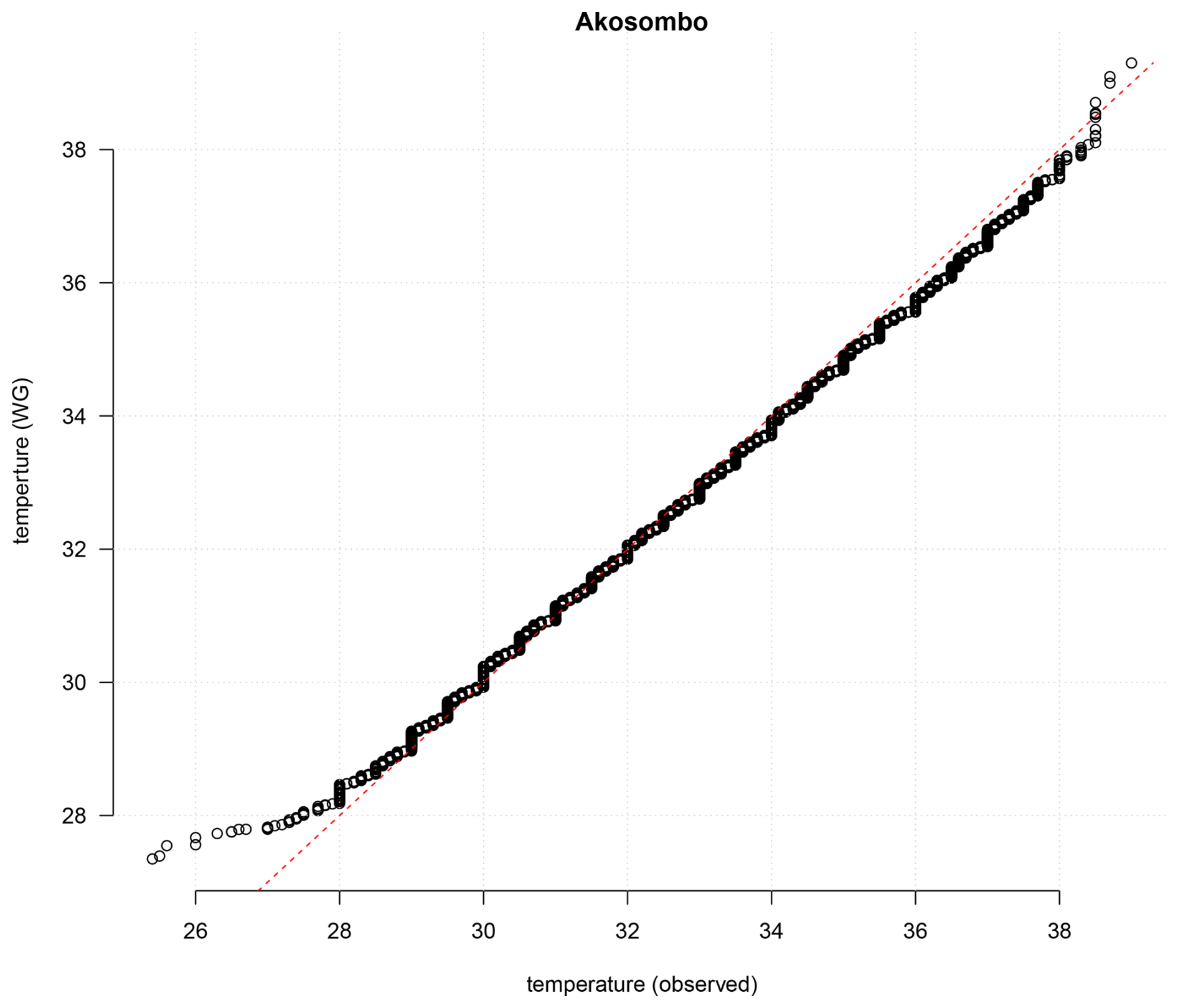
Figure 8 A quantile-quantile plot presenting test results for the simple WG for daily maximum temperature at Akosombo in Ghana. There was a some discrepancy in the lowest temperatures, but otherwise a good match with the observations.

The temperature-based WG was tested on a number of sites in Norway with freely available long temperature records (see Benestad, 2026b) where its skill was assessed through quantile-quantile plots of simulated temperatures against the original observations. Figure 9 shows two examples from Oslo and Tromsø, and the results indicated that the skill of reproducing the temperature amplitudes varied with location.

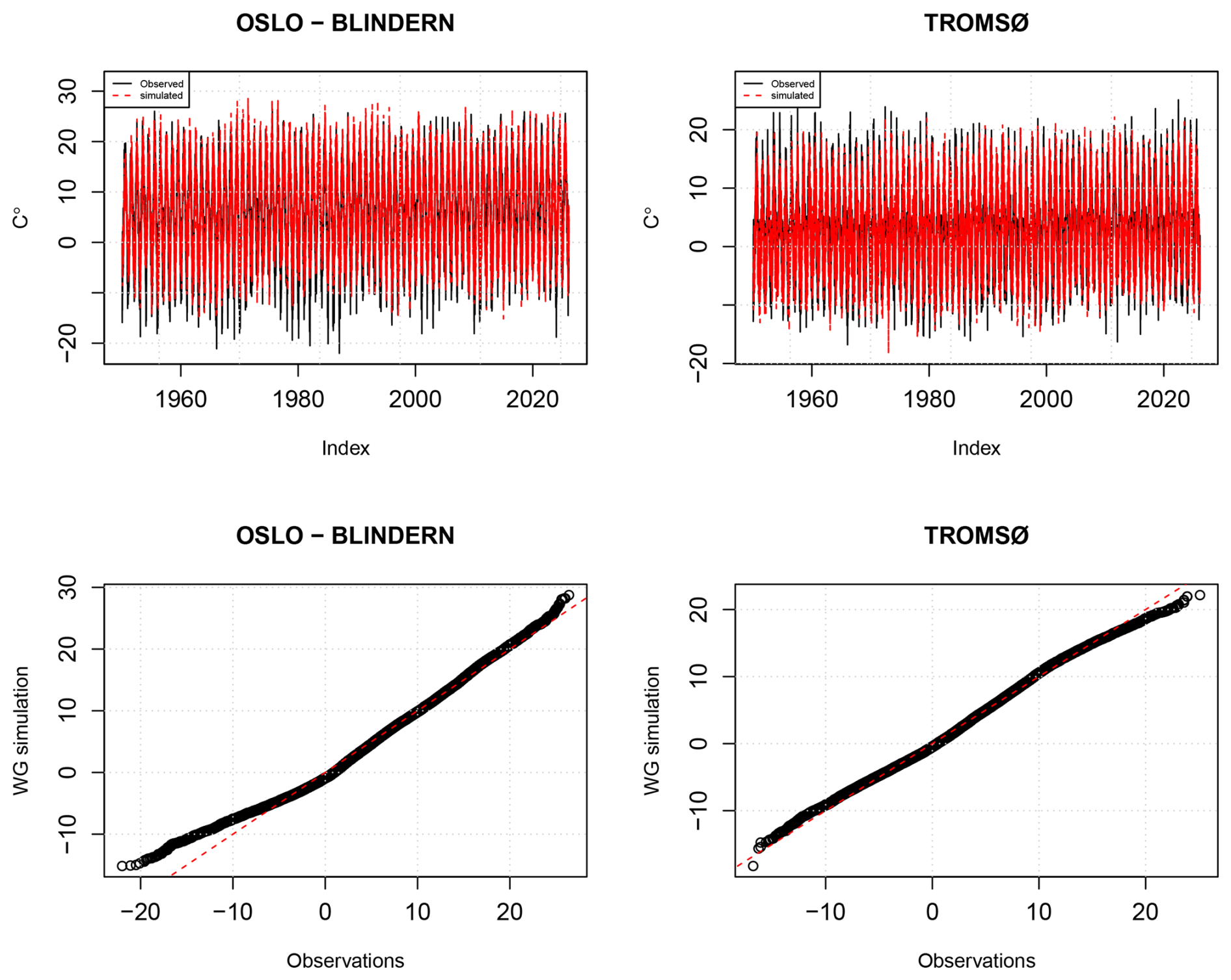
Figure 9 Examples of weather generator simulations for daily mean temperature in Oslo and Tromsø (upper pans) and an evaluation of the temperature amplitudes in the shape of quantilequantile plots (lower panels).

4 Discussion

The simple WGs for precipitation and temperature have been designed for single series. It is possible to provide precipitation projections for several sites within a region where the annual or seasonal statistics are spatially consistent if the downscaled results use a principal component analysis (PCA) as a basis for its predictands f_w and μ (Benestad et al., 2015a), but this solution does not apply to the daily sequences within the individual years. Hence, while they take annual statistics as input, which may correlate between nearby sites, they don't take into account possible systematic overlap between adjacent sites associated with daily precipitation or temperature with sufficiently large spatial scales. Furthermore, the WGs don't take into account potential correlation between daily precipitation and temperature in their simplest applications, but in some cases there is no clear correlation between the two, such as in Akosombo (Fig. 10), so that the different variables may be generated by different WG simulations. Many sites only measure rainfall or temperature and not both, which also makes it tricky to consider pairs of temperature and precipitation anyway. This issue is not only affecting ESD, as the covariance between daily temperature and precipitation also may be a problem with RCMs which may reproduce biased bi-variate statistical distributions (Benestad and Haugen, 2007).

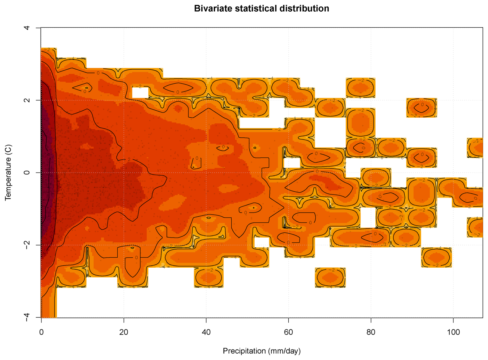
Figure 10 A bivariate statistical distribution or daily rainfall and daily mean temperature at Akosombo in Ghana shows that there is little covariance between the two variables.

Since the WG for precipitation has been designed to reproduce prescribed wet-day frequency and wet-day mean precipitation either aggregated over the entire period or on an annual basis, the purpose of comparing those statistics with observations is to provide a “sanity test” to see that the routine works as it should. The sequencing of the daily amounts is random in the WG simulations, and since the number of spells are fewer than the length of the simulated time series itself, we must expect a higher degree of random statistical fluctuations in the spell statistics. For all intents and purposes, the spell durations of the observations may also be regarded as random if the observation can be considered as one realisation of many possible. One interesting question is why there is such an underestimation of dry and wet spell durations in the data from the WG, at least for Bjørnholt, and one explanation may be that when the wet-day frequency climatology is flat ($f_{\mathrm{w}}\in [\mathrm{0.29},\mathrm{0.42}]$) then the wet days tend to spread more out during a year, as opposed to when they are concentrated into more distinct and shorter rainy seasons.

The underestimation of wet-spell and dry-spell duration is an important limitation, and may affect the estimation of hydrological model outputs, especially run-off generation, antecedent moisture, flood peaks, and drought duration. This shortcoming affects the simple WG for precipitation without further considerations, and it may be possible to subsequently move single wet days (i.e. reshuffle the data) simulated by the WG to the closest group of consecutive wet days (i.e. clustering the wet days) so that they also improve the spell length statistics (see Benestad, 2026b). The need to cluster dry and wet days respectively appears to depend on the chosen location and the wet-day frequency climatology (whether there are rainy seasons or not), and can be controlled in the model through an argument to its R call (setting the arguments 'cluster=TRUE' and assigning a value to 'prob_shift') as it is also useful to have the very simple type for when the spell durations don’t matter. It’s important to take into account that the timing of wet and dry days has up to this point been based on the wet-day frequency climatology, since a desire has been to reproduce the rainy seasons, so some modest shuffling of wet and dry days sometimes needs to be carried out in a fashion that doesn’t artificially change the climatologies (rainy seasons) for the sake of getting good spell duration statistics. If the climatologies are flat anyway, then they may not be strongly influenced by such reshuffling.

Although these simple WGs have been designed to be able to take into account correlations in annual f_w and μ, the lack of dependence between simulated daily precipitation and temperature may matter for snow and evapotranspiration applications. There may be some options for the daily data, however, and since the time structure of the daily temperature simulations is expected to be realistic due to the preservation of spectral power in the Fourier series, the simulated temperature may be used to guide the timing of daily precipitation that has biases when it comes to spell duration statistics. One possibility is to use a pair of temperature and precipitation series from the same location and reshuffle wet days based on e.g. a moving 15 d window and a rank analysis of temperature and precipitation within this segment. Furthermore, a copula can introduced to improve the daily timing and co-occurrence of rainfall by coupling it to a joint dependence structure of temperature and precipitation independently of their individual marginal probability distributions (Cong and Brady, 2012; Van De Velde et al., 2023). These consideration are beyond the scope of this documentation of the simple WGs, but are more relevant for specific application of WGs for the use in hydrological modelling, and hence left for future research and development.

It is also useful to keep in mind that some variables may not change much or may be associated with a weak response in the impact model, and in this case, they may be represented by surrogate noise. For instance, Mtongori et al. (2015) used a crop model to evaluate the effect of either changed temperature or rainfall on maize crops, and found the model to be more sensitive to temperature change. There are other elements such as wind and short-wave radiation (sunlight) which may affect local hydrology, but there is no clear evidence that wind speed and direction are expected to change substantially. Short-wave radiation is affected by cloudiness and aerosols, and is not expected to change as a direct consequence of an increased greenhouse effect (but may nevertheless be affected by altered anthropogenic emissions of for example sulphur and soot). In such cases, surrogate variables may be used, such as the output of similar weather generators that reproduce their salient characteristics.

The simple WGs presented herein were not designed to simulate changes in climatological profiles, and when annual statistics is used as input, it is also assumed that the climatology is stationary. However, a more advanced strategy could be to use monthly statistics as input that may make it possible to simulate changes to the climatological profiles, e.g. based on downscaled monthly estimates of f_w and μ.

5 Conclusions

In summary, a simple weather generator developed for the SPRINGS project facilitates a link between the downscaled precipitation statistics from global climate models and hydrological models that require daily rainfall as input. It can take downscaled wet-day frequency f_w and wet-day mean precipitation μ for a single location or a group of locations as input and simulate daily precipitation with a change to those parameters. The simple weather generator for daily precipitation gives a reasonable reproduction of the observations from a single site, but nevertheless has some limitations when it comes to reproducing the statistics of the durations of wet and dry spells. Furthermore, it doesn't take into account dependencies to nearby daily precipitation or temperature unless the simulations are processed further. A companion simple weather generator for daily temperature that can use annual mean temperature as well as standard deviation as inputs is also evaluated, and the test results also indicate that it gives a reasonable reproduction of the observations. It too has some limitations since it assumes that the daily temperature anomalies are normally distributed which results in the lowest simulated temperatures often being too high.

Appendix A

Algorithm A1 A simple demonstration of the use of the WG.

## The WG is a part of the R-package 'esd' and this chunk installs the esd package if it's
 not already installed:

install.esd <- ("esd" %in% rownames(installed.packages()) == FALSE)
if (install.esd) {
  ## Install esd from GitHub:
  install.devtools <- ("devtools" %in% rownames(installed.packages()) == FALSE)
  if (install.devtools) {
    print('Need to install the devtools package')
    ## You need online access.
    install.packages('devtools', dependencies = TRUE)
  }
  library(devtools)
  ## Need the R-packages zoo and ncdf4
  install.zoo <- ("zoo" %in% rownames(installed.packages()) == FALSE)
  if (install.zoo) install.packages('devtools', dependencies = TRUE)
  install.ncdf4 <- ("ncdf4" %in% rownames(installed.packages()) == FALSE)
  if (install.ncdf4) install.packages('ncdf4', dependencies = TRUE)
  library(devtools)
  print('Now install the esd package')
  ## You need online access.
  install_github('metno/esd')
}

## activate the esd-package
library(esd)
## Get the WG help page with examples - also use '?WG' for help pages on WG()
data(bjornholt)
## Demo run
z <- WG(bjornholt)
## simulate a hypothetical climate with fewer but more intensive rainy days
x <- WG(bjornholt,fw=wetfreq(z) - 0.1,mu=wetmean(z) + 2)
index(x) <- index(x) - index(x)[1] + as.Date('2050-01-01')
plot(zoo(combine.stations(z,x)),plot.type='single',col=c('black','grey'))

Algorithm A2 More advanced demonstration of the use of the WG.

## Retrieve gridded key annual rainfall statistics for the Nordic countries from
 thredds/OpenDap
lons <- lon(bjornholt) + c(-5,5)
lats <- lat(bjornholt) + c(-5,5)
thredds.path <- 'https://thredds.met.no/thredds/dodsC/metusers/rasmusb/'
mu.url <- 'mu_DSEns_Nordics_4seasons_1950-2100_ssp370.nc'
fw.url <- 'fw_DSEns_Nordics_4seasons_1950-2100_ssp370.nc'
param <- ncvars(paste0(thredds.path,mu.url))
## Get the ensemble mean and standard deviation
mu.m <- regrid(retrieve(paste0(thredds.path,mu.url),param=param[1],
                        lon=lons,lat=lats),bjornholt)
mu.s <- regrid(retrieve(paste0(thredds.path,mu.url),param=param[2],
                        lon=lons,lat=lats),bjornholt)
param <- ncvars(paste0(thredds.path,fw.url))
fw.m <- regrid(retrieve(paste0(thredds.path,fw.url),param=param[1],
                        lon=lons,lat=lats),bjornholt)
fw.s <- regrid(retrieve(paste0(thredds.path,fw.url),param=param[2],
                        lon=lons,lat=lats),bjornholt)
## generate a plausbile time series based on the smooth ensemble mean
## and random annual fluctuations based on the ensemble standard deviation
mu <- annual(mu.m + rnorm(length(mu.s))*mu.s)
fw <- annual(fw.m + rnorm(length(fw.s))*fw.s)
z.bjornholt <- WG(bjornholt,mu=mu,fw=fw)
plot(combine.stations(bjornholt,z.bjornholt))