Development and improvement of a nonhydrostatic spectral model using non-constant coefficient semi-implicit and vertically conservative semi-Lagrangian schemes

A two-dimensional x–z nonhydrostatic spectral model has been developed as a simpler framework for testing and improving numerical methods before they are applied to the corresponding global model. The model uses non-constant coefficient semi-implicit and vertically conservative semi-Lagrangian schemes and is computationally efficient by allowing for long timesteps in simulations. The model incorporates several improvements related to free-slip surface boundary conditions, prognostic variables in spectral space, and the semi-Lagrangian and semi-implicit schemes. These improvements enhance numerical stability, especially in cases with steep orography, and improve model results. The model was tested with various test cases (e.g., mountain wave test cases), confirming that a single recalculation of the non-constant coefficient linear terms is usually sufficient to stably solve the equations associated with the non-constant coefficient semi-implicit scheme, even in the cases with a steep mountain with an average slope of 45°. The model also ran stably even in the case of an extremely steep mountain with an average slope of 63.4° by performing several iterations using the preconditioned general conjugate residual method. In all these cases, good results were obtained with long timesteps.

1 Introduction

The global spectral atmospheric models used by the Japan Meteorological Agency (JMA, 2019) and Meteorological Research Institute (MRI; Yukimoto et al., 2011, 2019) are hydrostatic. In these models, a two-time-level, semi-implicit semi-Lagrangian scheme is used to allow for longer timesteps, and a vertically conservative semi-Lagrangian scheme (Yoshimura and Matsumura, 2003; Katayama et al., 2005; Yoshimura and Matsumura, 2005; Yukimoto et al., 2011) is used to improve conservation, which reduces the temperature biases around the tropical tropopause (Yoshimura and Matsumura, 2003). The reduced grid (Juang, 2004; Miyamoto, 2006, 2009) is used to save computational cost in the JMA atmospheric model and has also been introduced into the latest development version of the MRI atmospheric model. The advantage of the spectral method used in the hydrostatic models is that, in addition to its good accuracy, the linear simultaneous equations associated with the semi-implicit scheme can be easily solved in spectral space without iterations.

We have been developing a nonhydrostatic option for high-resolution simulations with the MRI global atmospheric spectral model. The prognostic equations used in the nonhydrostatic option are essentially the same as those in the ALADIN-NH (Non-Hydrostatic version of Aire Limitée Adaptation Dynamique Développement InterNational) nonhydrostatic limited-area spectral model (Bubnová et al., 1995; Geleyn and Bubnová, 1997; Bénard et al., 2010) and those in the nonhydrostatic version of the IFS (Integrated Forecasting System) global spectral model (Wedi and Smolarkiewicz, 2009; Dueben et al., 2020; Wedi et al., 2020; Vivoda et al., 2026). However, there are some differences in time discretization. In the ALADIN-NH and nonhydrostatic IFS, an iterative centered-implicit (ICI) scheme (Bénard, 2003; Bénard et al., 2005, 2010; Vivoda et al., 2026) is used to improve model stability, where all terms are recalculated at each iteration. In the nonhydrostatic option in the MRI model, a non-constant coefficient semi-implicit scheme is used, where only non-constant coefficient linear terms are recalculated at each iteration and, therefore, the computational cost at each iteration is lower than that for the ICI scheme. A fast-convergent iterative method, such as the general conjugate residual (GCR) method (Eisenstat et al., 1983) with preconditioning, can be used to solve the linear equations associated with the non-constant coefficient semi-implicit scheme in grid models (e.g., Skamarock et al., 1997; Thomas et al., 2003) and can also be used in the spectral model (Yoshimura, 2012, Appendix E3). A single-recalculation method can also be used in the spectral model (Appendix E2).

The early version of the nonhydrostatic option in the previous MRI global spectral model was briefly described by Yoshimura (2012). An option using double Fourier series instead of spherical harmonics as spectral basis functions was also developed to improve the computational efficiency at high resolution (Yoshimura and Matsumura, 2005; Yoshimura, 2012, 2022). Nakano et al. (2017) presented the results of typhoon simulations in the previous MRI model using the early versions of the nonhydrostatic and double Fourier series options (DFSM), along with the results of the Nonhydrostatic ICosahedral Atmospheric Model (NICAM) and the Multi-Scale Simulator for the Geoenvironment (MSSG).

To test and improve the nonhydrostatic spectral dynamical core, we have developed a nonhydrostatic spectral two-dimensional x–z model. The model is essentially a two-dimensional version of the corresponding three-dimensional global model using spherical harmonics or double Fourier series. It provides a simpler framework for testing and improving numerical methods before they are applied to the global model. In the model, several modifications have been introduced, including improved treatment of the free-slip surface boundary conditions, modification of the prognostic variables in spectral space, and improvements related to the semi-Lagrangian and the semi-implicit schemes. The model was tested with various test cases, which confirmed that these modifications enhance the numerical stability in cases with steep orography, reduce the number of iterations needed to solve the non-constant coefficient semi-implicit equations, and improve the results.

The remainder of the paper is organized as follows. Section 2 describes the prognostic equations for the global and the two-dimensional x–z nonhydrostatic spectral models and how to discretize these, including the free-slip surface boundary conditions. Section 3 shows the results of test cases of the two-dimensional x–z nonhydrostatic model. Section 4 presents the conclusions of this study and considers future work.

2 Nonhydrostatic model

Section 2.1 and Appendix A describe the mass-based hybrid vertical coordinate system. Section 2.2 describes the prognostic equations for the global and two-dimensional x–z nonhydrostatic spectral models, and Sect. 2.3 describes an improvement related to the free-slip surface boundary conditions. Section 2.4 and 2.5 and Appendix C describe the temporal and vertical discretization of the prognostic equations. Section 2.6 describes the time-integration procedure, and Sect. 2.7 describes the computational cost of spectral transforms. Appendix B describes the vertically conservative semi-Lagrangian scheme including several improvements such as a spatially averaged Eulerian treatment of mountains and a semi-Lagrangian treatment of pressure change due to horizontal advection. Appendix D describes the spectral transform of the prognostic variables, and Appendix E shows how to solve the equations for the non-constant coefficient semi-implicit scheme. Appendix F describes the Rayleigh damping.

2.1 Vertical coordinate

A mass-based vertical coordinate (Simmons and Burridge, 1981; Laprise, 1992; Bubnová et al., 1995) is used. The hydrostatic pressure π is given by

$$\begin{array}{}\text{(1)}& \mathit{\pi }=A\left(\mathit{\eta }\right)+B\left(\mathit{\eta }\right){\mathit{\pi }}_{\mathrm{s}},\mathrm{0}\le \mathit{\eta }\le \mathrm{1},\end{array}$$

where η is a hybrid vertical coordinate and π_s is the surface hydrostatic pressure. By discretizing Eq. (1) vertically, the hydrostatic pressure at the half level $k-\mathrm{1}/\mathrm{2}$ is given by

$$\begin{array}{}\text{(2)}& {\mathit{\pi }}_{k-\mathrm{1}/\mathrm{2}}=A_{k-\mathrm{1}/\mathrm{2}}+B_{k-\mathrm{1}/\mathrm{2}}{\mathit{\pi }}_{\mathrm{s}},\mathrm{1}\le k\le K+\mathrm{1},\end{array}$$

where ${\mathit{\pi }}_{\mathrm{1}/\mathrm{2}}=\mathit{\pi }\left(\mathit{\eta }=\mathrm{1}\right)={\mathit{\pi }}_{\mathrm{s}}$, ${\mathit{\pi }}_{K+\mathrm{1}/\mathrm{2}}=\mathit{\pi }\left(\mathit{\eta }=\mathrm{0}\right)=\mathrm{0.0}$, and K is the number of vertical full levels. The full level k represents the vertical layer between ${\mathit{\pi }}_{k-\mathrm{1}/\mathrm{2}}$ and ${\mathit{\pi }}_{k+\mathrm{1}/\mathrm{2}}$. The hydrostatic pressure depth Δπ_k at the full level k is given by

$$\begin{array}{}\text{(3a)}& {\displaystyle }\mathrm{\Delta }{\mathit{\pi }}_k\equiv {\mathit{\pi }}_{k-\mathrm{1}/\mathrm{2}}-{\mathit{\pi }}_{k+\mathrm{1}/\mathrm{2}}=\mathrm{\Delta }{A}_k+\mathrm{\Delta }{B}_k{\mathit{\pi }}_{\mathrm{s}},\text{(3b)}& {\displaystyle }\mathrm{\Delta }{A}_k\equiv A_{k-\mathrm{1}/\mathrm{2}}-A_{k+\mathrm{1}/\mathrm{2}},\text{(3c)}& {\displaystyle }\mathrm{\Delta }{B}_k\equiv B_{k-\mathrm{1}/\mathrm{2}}-B_{k+\mathrm{1}/\mathrm{2}}.\end{array}$$

An example of how to obtain $A_{k-\mathrm{1}/\mathrm{2}}$ and $B_{k-\mathrm{1}/\mathrm{2}}$ is shown in Appendix A, which is used in the two-dimensional x–z nonhydrostatic model in Sect. 3.

2.2 Nonhydrostatic equations

The following prognostic equations are used, which are essentially the same as in Bubnová et al. (1995):

$$\begin{array}{}\text{(4)}& {\displaystyle }\mathcal{P}\equiv \left(p-\mathit{\pi }\right)/\mathit{\pi },\text{(5)}& {\displaystyle }\mathcal{Q}\equiv \ln \left(p/\mathit{\pi }\right)=\ln \left(\mathrm{1}+\mathcal{P}\right)\text{(6)}& {\displaystyle }m\equiv \partial \mathit{\pi }/\partial \mathit{\eta },\end{array}$$

$$\begin{array}{}\text{(7a)}& {\displaystyle \frac{\mathrm{d}\mathit{v}}{\mathrm{d}t}}={\mathit{F}}_v,\text{(7b)}& {\displaystyle }{\mathit{F}}_v\equiv -RT\left[\mathrm{\nabla }\ln \mathit{\pi }+\mathrm{\nabla }\mathcal{Q}\right]-\mathrm{\nabla }\mathrm{\Phi }-{\displaystyle \frac{\mathrm{1}}{m}}{\displaystyle \frac{\partial \left(\mathit{\pi }\mathcal{P}\right)}{\partial \mathit{\eta }}}\mathrm{\nabla }\mathrm{\Phi },\end{array}$$

$$\begin{array}{}\text{(8a)}& {\displaystyle \frac{\mathrm{d}w}{\mathrm{d}t}}=F_w,\text{(8b)}& {\displaystyle }{F}_w\equiv {\displaystyle \frac{g}{m}}{\displaystyle \frac{\partial \left(\mathit{\pi }\mathcal{P}\right)}{\partial \mathit{\eta }}},\end{array}$$

$$\begin{array}{}\text{(9a)}& {\displaystyle \frac{\mathrm{dln}T}{\mathrm{d}t}}=F_{\ln T},\text{(9b)}& {\displaystyle }{F}_{\ln T}\equiv -{\displaystyle \frac{R}{c_{\mathrm{v}}}}{D}_{\mathrm{3}},\end{array}$$

$$\begin{array}{}\text{(10a)}& {\displaystyle \frac{\mathrm{d}\mathcal{Q}}{\mathrm{d}t}}\left(={\displaystyle \frac{\mathrm{dln}\left(\mathrm{1}+\mathcal{P}\right)}{\mathrm{d}t}}\right)=F_{\mathcal{Q}},\text{(10b)}& {\displaystyle }{F}_{\mathcal{Q}}\equiv -{\displaystyle \frac{\mathrm{1}}{\mathit{\pi }}}{\displaystyle \frac{\mathrm{d}\mathit{\pi }}{\mathrm{d}t}}-{\displaystyle \frac{c_{\mathrm{p}}}{c_{\mathrm{v}}}}{D}_{\mathrm{3}},\end{array}$$

$$\begin{array}{}\text{(11)}& {\displaystyle \frac{\partial }{\partial t}}\left({\displaystyle \frac{\partial \mathit{\pi }}{\partial \mathit{\eta }}}\right)+\mathrm{\nabla }\cdot \left(\mathit{v}{\displaystyle \frac{\partial \mathit{\pi }}{\partial \mathit{\eta }}}\right)+{\displaystyle \frac{\partial }{\partial \mathit{\eta }}}\left(\dot{\mathit{\eta }}{\displaystyle \frac{\partial \mathit{\pi }}{\partial \mathit{\eta }}}\right)=\mathrm{0},\text{(12)}& {\displaystyle }\mathrm{\Phi }={\mathrm{\Phi }}_{\mathrm{s}}+\underset{\mathit{\eta }}{\overset{\mathrm{1}}{\int }}\left[{\displaystyle \frac{RT}{\left(\mathrm{1}+\mathcal{P}\right)\mathit{\pi }}}m\right]\mathrm{d}{\mathit{\eta }}^{\prime },\text{(13)}& {\displaystyle }\begin{array}{rl}{D}_{\mathrm{3}}& \equiv \mathrm{\nabla }\cdot \mathit{v}+{\displaystyle \frac{\left(\mathrm{1}+\mathcal{P}\right)\mathit{\pi }}{RT}}{\displaystyle \frac{\mathrm{1}}{m}}\mathrm{\nabla }\mathrm{\Phi }\cdot {\displaystyle \frac{\partial \mathit{v}}{\partial \mathit{\eta }}}\\ & -{\displaystyle \frac{\left(\mathrm{1}+\mathcal{P}\right)\mathit{\pi }}{RT}}{\displaystyle \frac{g}{m}}{\displaystyle \frac{\partial w}{\partial \mathit{\eta }}},\end{array}\end{array}$$

where t is time, p is pressure, T is temperature, v is horizontal wind, w is vertical wind, Φ is geopotential, Φ_s is surface geopotential, D₃ is three-dimensional divergence, R is the gas constant, c_p is the specific heat capacity at a constant pressure, c_v is the specific heat capacity at a constant volume, and ∇ is the horizontal gradient on constant η surfaces. The Coriolis term is omitted in Eq. (7a).

Almost the same prognostic equations are often used in nonhydrostatic spectral models. An advantage of these equations is that they allow similar formulations to be used in hydrostatic and nonhydrostatic models. Another advantage of these equations is that they allow the simultaneous equations associated with the semi-implicit scheme to be efficiently solved in spectral models. In this paper, the prognostic equations are discretized in time using a semi-implicit scheme with constant coefficient and non-constant coefficient linear terms (Sect. 2.4 and 2.5). The prognostic variables in spectral space are selected to improve numerical stability (Sect. 2.5). The simultaneous equations associated with the constant-coefficient linear terms can be easily solved in spectral space (Step 3 in Sect. 2.6). By utilizing this solver, the simultaneous equations including the non-constant-coefficient linear terms can also be efficiently solved (Step 4 in Sect. 2.6).

2.3 Improved treatment of the surface boundary conditions

Free-slip rigid surface boundary conditions can be written as follows (Bubnová et al., 1995; Geleyn and Bubnová, 1997; Bénard et al., 2010):

$$\begin{array}{}\text{(14)}& {\displaystyle }{w}_{\mathrm{s}}={\displaystyle \frac{\mathrm{1}}{g}}{\mathit{v}}_{\mathrm{s}}\cdot \mathrm{\nabla }{\mathrm{\Phi }}_{\mathrm{s}}={\displaystyle \frac{\mathrm{1}}{g}}{\mathit{v}}_{\mathrm{1}}\cdot \mathrm{\nabla }{\mathrm{\Phi }}_{\mathrm{s}},\text{(15)}& {\displaystyle }{\left[{\displaystyle \frac{\mathrm{1}}{m}}{\displaystyle \frac{\partial \left(\mathit{\pi }\mathcal{P}\right)}{\partial \mathit{\eta }}}\right]}_{\mathrm{s}}={\displaystyle \frac{\mathrm{1}}{g}}{\displaystyle \frac{\mathrm{d}{w}_{\mathrm{s}}}{\mathrm{d}t}},\end{array}$$

where the subscript s denotes the value at the surface, the subscript 1 denotes the value at the lowest full level k=1, and v_s=v₁ is assumed. Substituting Eq. (14) into Eq. (15) gives the following equation (Bubnová et al., 1995):

$$\begin{array}{}\text{(16)}& \begin{array}{rl}{\left[{\displaystyle \frac{\mathrm{1}}{m}}{\displaystyle \frac{\partial \left(\mathit{\pi }\mathcal{P}\right)}{\partial \mathit{\eta }}}\right]}_{\mathrm{s}}& ={\displaystyle \frac{\mathrm{1}}{g^{\mathrm{2}}}}[{\displaystyle \frac{\mathrm{d}{\mathit{v}}_{\mathrm{1}}}{\mathrm{d}t}}\cdot \mathrm{\nabla }{\mathrm{\Phi }}_{\mathrm{s}}+{u_{\mathrm{1}}}^{\mathrm{2}}{\displaystyle \frac{\partial }{\partial x}}{\displaystyle \frac{\partial {\mathrm{\Phi }}_{\mathrm{s}}}{\partial x}}\\ & +u_{\mathrm{1}}{v}_{\mathrm{1}}\left({\displaystyle \frac{\partial }{\partial x}}{\displaystyle \frac{\partial }{\partial y}}+{\displaystyle \frac{\partial }{\partial y}}{\displaystyle \frac{\partial }{\partial x}}\right){\mathrm{\Phi }}_{\mathrm{s}}\\ & +{v_{\mathrm{1}}}^{\mathrm{2}}{\displaystyle \frac{\partial }{\partial y}}{\displaystyle \frac{\partial {\mathrm{\Phi }}_{\mathrm{s}}}{\partial y}}],\end{array}\end{array}$$

where x and y are the horizontal axes, and u₁ and v₁ are the x and y components of v₁, respectively. In spherical coordinates, $\partial /\partial x=\mathrm{1}/\left(a\cos \mathit{\varphi }\right)\cdot \partial /\partial \mathit{\lambda }$ and $\partial /\partial y=\mathrm{1}/a\cdot \partial /\partial \mathit{\varphi }$, where λ is the longitude, ϕ is the latitude, and a is the radius of the sphere. Equation (7) can be discretized at the lowest full level as follows:

$$\begin{array}{}\text{(17)}& \begin{array}{rl}{\displaystyle \frac{\mathrm{d}{\mathit{v}}_{\mathrm{1}}}{\mathrm{d}t}}& ={\left\{-RT\left[\mathrm{\nabla }\ln \mathit{\pi }+\mathrm{\nabla }\mathcal{Q}\right]-\mathrm{\nabla }\mathrm{\Phi }\right\}}_{\mathrm{1}}\\ & -{\displaystyle \frac{\mathrm{1}}{\mathrm{2}}}\left\{{\left[{\displaystyle \frac{\mathrm{1}}{m}}{\displaystyle \frac{\partial \left(\mathit{\pi }\mathcal{P}\right)}{\partial \mathit{\eta }}}\right]}_{\mathrm{s}}+{\left[{\displaystyle \frac{\mathrm{1}}{m}}{\displaystyle \frac{\partial \left(\mathit{\pi }\mathcal{P}\right)}{\partial \mathit{\eta }}}\right]}_{\mathrm{1}+\mathrm{1}/\mathrm{2}}\right\}\mathrm{\nabla }{\mathrm{\Phi }}_{\mathrm{1}}.\end{array}\end{array}$$

It can be considered that Eqs. (16) and (17) are simultaneous equations for variables $\mathrm{d}{\mathit{v}}_{\mathrm{1}}/\mathrm{d}t$ and ${\left[\mathrm{1}/m\cdot \partial \left(\mathit{\pi }\mathcal{P}\right)/\partial \mathit{\eta }\right]}_{\mathrm{s}}$. Substituting Eq. (17) into Eq. (16) gives

$$\begin{array}{}\text{(18)}& \begin{array}{rl}& {\left[{\displaystyle \frac{\mathrm{1}}{m}}{\displaystyle \frac{\partial \left(\mathit{\pi }\mathcal{P}\right)}{\partial \mathit{\eta }}}\right]}_{\mathrm{s}}=\mathit{\left\{}\right[{\left[-RT\left(\mathrm{\nabla }\ln \mathit{\pi }+\mathrm{\nabla }\mathcal{Q}\right)-\mathrm{\nabla }\mathrm{\Phi }\right]}_{\mathrm{1}}\\ & -{\displaystyle \frac{\mathrm{1}}{\mathrm{2}}}{\left[{\displaystyle \frac{\mathrm{1}}{m}}{\displaystyle \frac{\partial \left(\mathit{\pi }\mathcal{P}\right)}{\partial \mathit{\eta }}}\right]}_{\mathrm{1}+\mathrm{1}/\mathrm{2}}\mathrm{\nabla }{\mathrm{\Phi }}_{\mathrm{1}}]\cdot \mathrm{\nabla }{\mathrm{\Phi }}_{\mathrm{s}}\\ & +{u_{\mathrm{1}}}^{\mathrm{2}}{\displaystyle \frac{\partial }{\partial x}}{\displaystyle \frac{\partial {\mathrm{\Phi }}_{\mathrm{s}}}{\partial x}}+u_{\mathrm{1}}{v}_{\mathrm{1}}\left({\displaystyle \frac{\partial }{\partial x}}{\displaystyle \frac{\partial }{\partial y}}+{\displaystyle \frac{\partial }{\partial y}}{\displaystyle \frac{\partial }{\partial x}}\right){\mathrm{\Phi }}_{\mathrm{s}}\\ & +{v_{\mathrm{1}}}^{\mathrm{2}}{\displaystyle \frac{\partial }{\partial y}}{\displaystyle \frac{\partial {\mathrm{\Phi }}_{\mathrm{s}}}{\partial y}}\mathit{\}}/\mathit{\{}{g}^{\mathrm{2}}+{\displaystyle \frac{\mathrm{1}}{\mathrm{2}}}\left[{\displaystyle \frac{\partial {\mathrm{\Phi }}_{\mathrm{s}}}{\partial x}}{\displaystyle \frac{\partial {\mathrm{\Phi }}_{\mathrm{1}}}{\partial x}}+{\displaystyle \frac{\partial {\mathrm{\Phi }}_{\mathrm{s}}}{\partial y}}{\displaystyle \frac{\partial {\mathrm{\Phi }}_{\mathrm{1}}}{\partial y}}\right]\mathit{\}}.\end{array}\end{array}$$

Substituting Eq. (18) into Eq. (17) gives the equation for $\mathrm{d}{\mathit{v}}_{\mathrm{1}}/\mathrm{d}t$.

In the two-dimensional x–z model, v=0 and $\partial /\partial y=\mathrm{0}$. Substituting Eq. (16) into Eq. (17) leads to

$$\begin{array}{}\text{(19a)}& {\displaystyle \frac{\mathrm{d}{u}_{\mathrm{1}}}{\mathrm{d}t}}=-C{\displaystyle \frac{\mathrm{d}{u}_{\mathrm{1}}}{\mathrm{d}t}}+U,\text{(19b)}& {\displaystyle }C\equiv {\displaystyle \frac{\mathrm{1}}{\mathrm{2}}}{\displaystyle \frac{\partial }{\partial x}}\left({\displaystyle \frac{{\mathrm{\Phi }}_{\mathrm{s}}}{g}}\right){\displaystyle \frac{\partial }{\partial x}}\left({\displaystyle \frac{{\mathrm{\Phi }}_{\mathrm{1}}}{g}}\right),\end{array}$$

where U contains the remaining terms independent of $\mathrm{d}{u}_{\mathrm{1}}/\mathrm{d}t$. The coefficient C is about 0.5 when the slope of a mountain is 45° and about 2.0 when the slope is 63.4°. Therefore, $C\mathrm{d}{u}_{\mathrm{1}}/\mathrm{d}t$ on the right side of Eq. (19a) should be treated with caution. It is considered best to convert Eq. (19a) into the following equation for use:

$$\begin{array}{}\text{(20)}& {\displaystyle \frac{\mathrm{d}{u}_{\mathrm{1}}}{\mathrm{d}t}}={\displaystyle \frac{U}{\mathrm{1}+C}},\end{array}$$

which is the same as the equation obtained by substituting Eq. (18) into Eq. (17).

In the previous nonhydrostatic option of the global MRI model, the following equation was used instead of Eq. (18):

$$\begin{array}{}\text{(21)}& {\left[{\displaystyle \frac{\mathrm{1}}{m}}{\displaystyle \frac{\partial \left(\mathit{\pi }\mathcal{P}\right)}{\partial \mathit{\eta }}}\right]}_{\mathrm{s}}={\left[{\displaystyle \frac{\mathrm{1}}{m}}{\displaystyle \frac{\partial \left(\mathit{\pi }\mathcal{P}\right)}{\partial \mathit{\eta }}}\right]}_{\mathrm{3}/\mathrm{2}}.\end{array}$$

The approximation in Eq. (21) is not fully consistent with the surface boundary condition in Eq. (15). It was found that the new method using Eqs. (18) and (17) gives better results than the previous method that uses Eqs. (21) and (17) (Sect. 3.2).

2.4 Discretization with the non-constant coefficient semi-implicit semi-Lagrangian scheme

The prognostic equations (Eqs. 7–11) can be represented as follows:

$$\begin{array}{}\text{(22)}& {\displaystyle \frac{\mathrm{d}X}{\mathrm{d}t}}=F\left(X\right),\end{array}$$

where X represents the prognostic variables. By using the vertically conservative semi-Lagrangian scheme (Appendix B), the non-constant coefficient semi-implicit scheme, the Stable Extrapolation Two-Time-Level Scheme (SETTLS; Hortal, 2002), and second-order decentering (Rivest et al., 1994; Ritchie et al., 1995; Simmons and Temperton, 1997; Yukimoto et al., 2011; Yoshimura, 2022), Eq. (22) can be discretized in time as follows:

$$\begin{array}{}\text{(23a)}& {\displaystyle }\begin{array}{rl}{\displaystyle \frac{X^{+}-X_{\mathrm{D}}^{\mathrm{0}}}{\mathrm{\Delta }t}}& ={\displaystyle \frac{\mathrm{1}}{\mathrm{2}}}{\left[F^{\left(+\right)}+\mathit{\beta }\left(-L_{\mathrm{C}}^{\left(+\right)}+L_{\mathrm{C}}^{\mathrm{0}}\right)+\left(-L_{\mathrm{N}}^{\left(+\right)}+L_{\mathrm{N}}^{\mathrm{0}}\right)\right]}_{\mathrm{D}}\\ & +{\displaystyle \frac{\mathrm{1}}{\mathrm{2}}}\left[F^{\mathrm{0}}+\mathit{\beta }\left(L_{\mathrm{C}}^{+}-L_{\mathrm{C}}^{\mathrm{0}}\right)+\left(L_{\mathrm{N}}^{+}-L_{\mathrm{N}}^{\mathrm{0}}\right)\right],\end{array}\text{(23b)}& {\displaystyle }\begin{array}{rl}{F}^{\left(+\right)}& \equiv \mathrm{2}{F}^{\mathrm{0}}-F^{-},L_{\mathrm{C}}^{\left(+\right)}\equiv \mathrm{2}{L}_{\mathrm{C}}^{\mathrm{0}}-L_{\mathrm{C}}^{-},L_{\mathrm{N}}^{\left(+\right)}\\ & \equiv \mathrm{2}{L}_{\mathrm{N}}^{\mathrm{0}}-L_{\mathrm{N}}^{-},\end{array}\end{array}$$

where L_C and L_N represent the constant and non-constant coefficient linear terms, respectively, obtained by linearizing F; Δt is the timestep; the superscripts −, 0, and + are the past (t−Δt), present (t), and future (t+Δt) values, respectively; and the superscript (+) is the future value (t+Δt) extrapolated in time. The subscript D represents the departure point in calculating advection (Appendix B1). The non-constant coefficient linear terms are used because the third term on the right side of Eq. (7b) and the second term on the right side of Eq. (13) contain ∇Φ as a coefficient and cannot be linearized as constant coefficient linear terms. Since these terms are related to sound waves, the semi-implicit scheme with non-constant coefficient linear terms is used to allow long timesteps. The parameter β for second-order decentering is set to β=1.2 instead of 1.0. The parameter β applied to L_C is similar to that used in the second-order three-time-level semi-implicit semi-Lagrangian scheme of Ritchie et al. (1995).

Equation (23a) can be rewritten as follows:

$$\begin{array}{}\text{(23a')}& {\displaystyle }\begin{array}{rl}{\displaystyle \frac{X^{+}-X_{\mathrm{D}}^{\mathrm{0}}}{\mathrm{\Delta }t}}& ={\displaystyle \frac{\mathrm{1}}{\mathrm{2}}}\left[N_{\mathrm{D}}^{\left(+\right)}+N^{\mathrm{0}}\right]+{\displaystyle \frac{\mathrm{1}}{\mathrm{2}}}\left[L_{\mathrm{C},\mathrm{D}}^{\mathrm{0}}+L_{\mathrm{C}}^{+}\right]\\ & +{\displaystyle \frac{\mathrm{1}}{\mathrm{2}}}\left[L_{\mathrm{N},\mathrm{D}}^{\mathrm{0}}+L_{\mathrm{N}}^{+}\right]\\ & +{\displaystyle \frac{\mathit{\xi }}{\mathrm{2}}}\left[-\left(L_{\mathrm{C},\mathrm{D}}^{\left(+\right)}+L_{\mathrm{C}}^{\mathrm{0}}\right)+\left(L_{\mathrm{C},\mathrm{D}}^{\mathrm{0}}+L_{\mathrm{C}}^{+}\right)\right]\end{array}\text{(23c)}& {\displaystyle }N\equiv F-L_{\mathrm{C}}-L_{\mathrm{N}}\text{(23d)}& {\displaystyle }\mathit{\xi }\equiv \mathit{\beta }-\mathrm{1}\end{array}$$

When ξ=0, Eq. (23a') becomes the centered second-order semi-implicit semi-Lagrangian formulation with SETTLS extrapolation applied to the nonlinear residual term N at the departure point. In the formulation used here, the linear terms include not only L_C but also L_N.

When no distinction is made between the departure and arrival points in order to examine temporal accuracy, Eq. (23a') can be rewritten using Eq. (23b) as follows:

$$\begin{array}{}\text{(23e)}& \begin{array}{rl}{\displaystyle \frac{X^{+}-X^{\mathrm{0}}}{\mathrm{\Delta }t}}& ={\displaystyle \frac{\mathrm{1}}{\mathrm{2}}}\left[N^{\left(+\right)}+N^{\mathrm{0}}\right]+{\displaystyle \frac{\mathrm{1}}{\mathrm{2}}}\left[L_{\mathrm{N}}^{\mathrm{0}}+L_{\mathrm{N}}^{+}\right]\\ & +{\displaystyle \frac{\mathrm{1}}{\mathrm{2}}}\left[\left(\mathrm{1}+\mathit{\xi }\right)L_{\mathrm{C}}^{+}+\left(\mathrm{1}-\mathrm{2}\mathit{\xi }\right)L_{\mathrm{C}}^{\mathrm{0}}+\mathit{\xi }{L}_{\mathrm{C}}^{-}\right].\end{array}\end{array}$$

The temporal weighting of the constant-coefficient linear terms in Eq. (23e) is the same as that used in the second-order decentering formulations presented in Eqs. (12) and (14) of Rivest et al. (1994) and Eq. (38) of Simmons and Temperton (1997).

Although the terms $F^{\left(+\right)}+\mathit{\beta }\left(-L_{\mathrm{C}}^{\left(+\right)}+L_{\mathrm{C}}^{\mathrm{0}}\right)+\left(-L_{\mathrm{N}}^{\left(+\right)}+L_{\mathrm{N}}^{\mathrm{0}}\right)$ at the departure point in Eq. (23a) contain time-extrapolated values, the combination of these terms is interpolative in time. When $F=L_{\mathrm{C}}+L_{\mathrm{N}}$, that is, N=0, these terms become $\left(\mathrm{1}-\mathit{\xi }\right)L_{\mathrm{C}}^{\mathrm{0}}+\mathit{\xi }{L}_{\mathrm{C}}^{-}+L_{\mathrm{N}}^{\mathrm{0}}$. Here, $\left(\mathrm{1}-\mathit{\xi }\right)L_{\mathrm{C}}^{\mathrm{0}}+\mathit{\xi }{L}_{\mathrm{C}}^{-}$ represents a temporal interpolation between $L_{\mathrm{C}}^{\mathrm{0}}$ and $L_{\mathrm{C}}^{-}$ for $\mathrm{0}\le \mathit{\xi }\le \mathrm{1}$; $\mathit{\xi }=\mathit{\beta }-\mathrm{1}=\mathrm{0.2}$ is used here. Thus, the combination of SETTLS and second-order decentering with $\mathit{\beta }=\mathit{\xi }+\mathrm{1}$, which is a little larger than 1.0, can avoid time extrapolation, a potential source of instability. The use of β>1 can also enhance the stabilizing effect of the semi-implicit scheme by increasing the coefficient of $L_{\mathrm{C}}^{+}$. The results in Sect. 3.2 show that numerical stability is reduced when β is changed from 1.2 to 1.0. The factor β is applied only to the constant coefficient linear terms because its application to the non-constant coefficient linear terms does not improve numerical stability in the test cases in this paper.

In the vertically conservative semi-Lagrangian scheme (Appendix B), computation of the advection terms is divided into the horizontal and vertical directions, and the vertical transport (vertical remapping) is evaluated with a one-dimensional conservative semi-Lagrangian scheme (Appendices B2 and B3). The horizontal advection is calculated in the usual non-conservative way (Appendices B4 and B5), with several related improvements (Appendices B6–B8). A correction method (Priestley, 1993; Gravel and Staniforth, 1994) can be used for global conservation of mass and the tracers, but is not used here.

Equation (23a) can be converted as follows:

$$\begin{array}{}\text{(24a)}& {\displaystyle }{X}^{+}-{\displaystyle \frac{\mathit{\beta }\mathrm{\Delta }t}{\mathrm{2}}}{L}_{\mathrm{C}}^{+}-{\displaystyle \frac{\mathrm{\Delta }t}{\mathrm{2}}}{L}_{\mathrm{N}}^{+}=R_X\text{(24b)}& {\displaystyle }\begin{array}{rl}{R}_X& \equiv {\left[X^{\mathrm{0}}+{\displaystyle \frac{F^{\left(+\right)}+\mathit{\beta }\left(-L_{\mathrm{C}}^{\mathrm{0}}+L_{\mathrm{C}}^{-}\right)+\left(-L_{\mathrm{N}}^{\mathrm{0}}+L_{\mathrm{N}}^{-}\right)}{\mathrm{2}}}\mathrm{\Delta }t\right]}_{\mathrm{D}}\\ & +{\displaystyle \frac{F^{\mathrm{0}}+\mathit{\beta }\left(-L_{\mathrm{C}}^{\mathrm{0}}\right)+\left(-L_{\mathrm{N}}^{\mathrm{0}}\right)}{\mathrm{2}}}\mathrm{\Delta }t,\end{array}\end{array}$$

where R_X can be calculated explicitly.

2.5 Discretization of the nonhydrostatic prognostic equations

Using the discretization of Eq. (24), Eqs. (7)–(11) are discretized in time as follows:

$$\begin{array}{}\text{(25)}& {\displaystyle }{\mathit{\pi }}^{*}\equiv A\left(\mathit{\eta }\right)+B\left(\mathit{\eta }\right){\stackrel{\mathrm{‾}}{\mathit{\pi }}}_{\mathrm{s}},\text{(26)}& {\displaystyle }{m}^{*}\equiv \partial {\mathit{\pi }}^{*}/\partial \mathit{\eta },\end{array}$$

$$\begin{array}{}\text{(27a)}& {\displaystyle }{\mathit{v}}^{+}-{\displaystyle \frac{\mathit{\beta }\mathrm{\Delta }t}{\mathrm{2}}}{\mathit{L}}_{\mathrm{C},v}^{+}-{\displaystyle \frac{\mathrm{\Delta }t}{\mathrm{2}}}{\mathit{L}}_{\mathrm{N},v}^{+}={\mathit{R}}_v,\text{(27b)}& {\displaystyle }\begin{array}{rl}{\mathit{R}}_v& \equiv {\left[{\mathit{v}}^{\mathrm{0}}+{\displaystyle \frac{{\mathit{F}}_v^{\left(+\right)}+\mathit{\beta }\left(-{\mathit{L}}_{\mathrm{C},v}^{\mathrm{0}}+{\mathit{L}}_{\mathrm{C},v}^{-}\right)+\left(-{\mathit{L}}_{\mathrm{N},v}^{\mathrm{0}}+{\mathit{L}}_{\mathrm{N},v}^{-}\right)}{\mathrm{2}}}\mathrm{\Delta }t\right]}_{\mathrm{D}}\\ & +{\displaystyle \frac{{\mathit{F}}_v^{\mathrm{0}}+\mathit{\beta }\left(-{\mathit{L}}_{\mathrm{C},v}^{\mathrm{0}}\right)+\left(-{\mathit{L}}_{\mathrm{N},v}^{\mathrm{0}}\right)}{\mathrm{2}}}\mathrm{\Delta }t,\end{array}\text{(27c)}& {\displaystyle }{\mathit{L}}_{\mathrm{C},v}\equiv R\stackrel{\mathrm{‾}}{T}\left[{\mathcal{G}}^{*}\left(-\mathrm{\nabla }\ln T+\mathrm{\nabla }\mathcal{Q}\right)-\mathrm{\nabla }\mathcal{Q}-\mathrm{\nabla }\ln {\mathit{\pi }}_{\mathrm{s}}\right],\text{(27d)}& {\displaystyle }{\mathcal{G}}^{*}X\equiv \underset{\mathit{\eta }}{\overset{\mathrm{1}}{\int }}{\displaystyle \frac{m^{*}}{{\mathit{\pi }}^{*}}}X\mathrm{d}{\mathit{\eta }}^{\prime },\text{(27e)}& {\displaystyle }{\mathit{L}}_{\mathrm{N},v}\equiv -{\displaystyle \frac{\mathrm{1}}{m^{\mathit{\#}}}}{\displaystyle \frac{\partial \left({\mathit{\pi }}^{\mathit{\#}}\mathcal{P}\right)}{\partial \mathit{\eta }}}\mathrm{\nabla }{\mathrm{\Phi }}^{\mathit{\#}},\end{array}$$

$$\begin{array}{}\text{(28a)}& {\displaystyle }{w}^{+}=R_w,\text{(28b)}& {\displaystyle }{R}_w\equiv {\left[w^{\mathrm{0}}+{\displaystyle \frac{F_w^{\left(+\right)}}{\mathrm{2}}}\mathrm{\Delta }t\right]}_{\mathrm{D}}+{\displaystyle \frac{F_w^{\mathrm{0}}}{\mathrm{2}}}\mathrm{\Delta }t,\text{(28c)}& {\displaystyle }{w}_{\mathrm{s}}^{+}={\displaystyle \frac{\mathrm{1}}{g}}{\mathit{v}}_{\mathrm{1}}^{+}\cdot \mathrm{\nabla }{\mathrm{\Phi }}_{\mathrm{s}},\end{array}$$

$$\begin{array}{}\text{(29a)}& {\displaystyle }\ln T^{+}-{\displaystyle \frac{\mathit{\beta }\mathrm{\Delta }t}{\mathrm{2}}}{L}_{\mathrm{C},\ln T}^{+}=R_{\ln T},\text{(29b)}& {\displaystyle }\begin{array}{rl}{R}_{\ln T}& \equiv \ln T_{\mathrm{D}}^{\mathrm{0}}+{\left[{\displaystyle \frac{F_{\ln T}^{\left(+\right)}+\mathit{\beta }\left(-L_{\mathrm{C},\ln T}^{\mathrm{0}}+L_{\mathrm{C},\ln T}^{-}\right)}{\mathrm{2}}}\mathrm{\Delta }t\right]}_{\mathrm{D}}\\ & +{\displaystyle \frac{F_{\ln T}^{\mathrm{0}}+\mathit{\beta }\left(-L_{\mathrm{C},\ln T}^{\mathrm{0}}\right)}{\mathrm{2}}}\mathrm{\Delta }t,\end{array}\text{(29c)}& {\displaystyle }{L}_{\mathrm{C},\ln T}\equiv -{\displaystyle \frac{R}{c_{\mathrm{v}}}}\left(D+\widehat{\widehat{d}}\right),\end{array}$$

$$\begin{array}{}\text{(30a)}& {\displaystyle }{\mathcal{Q}}^{+}-{\displaystyle \frac{\mathit{\beta }\mathrm{\Delta }t}{\mathrm{2}}}{L}_{\mathrm{C},\mathcal{Q}}^{+}=R_{\mathcal{Q}},\text{(30b)}& {\displaystyle }\begin{array}{rl}{R}_{\mathcal{Q}}& \equiv {\left[\ln \left(\mathrm{1}+{\mathcal{P}}^{\mathrm{0}}\right)+{\displaystyle \frac{F_{\mathcal{Q}\left(\mathrm{div}\right)}^{\left(+\right)}+\mathit{\beta }\left(-L_{\mathrm{C},\mathcal{Q}}^{\mathrm{0}}+L_{\mathrm{C},\mathcal{Q}}^{-}\right)}{\mathrm{2}}}\mathrm{\Delta }t\right]}_{\mathrm{D}}\\ & +{\displaystyle \frac{F_{\mathcal{Q}\left(\mathrm{div}\right)}^{\mathrm{0}}+\mathit{\beta }\left(-L_{\mathrm{C},\mathcal{Q}}^{\mathrm{0}}\right)}{\mathrm{2}}}\mathrm{\Delta }t+F_{\mathcal{Q}\left(\mathrm{adv}\right)}\mathrm{\Delta }t,\end{array}\text{(30c)}& {\displaystyle }{F}_{\mathcal{Q}\left(\mathrm{div}\right)}+F_{\mathcal{Q}\left(\mathrm{adv}\right)}=F_{\mathcal{Q}},\text{(30d)}& {\displaystyle }{L}_{\mathrm{C},\mathcal{Q}}\equiv {\mathcal{S}}^{*}D-{\displaystyle \frac{c_{\mathrm{p}}}{c_{\mathrm{v}}}}\left(D+\widehat{\widehat{d}}\right),\text{(30e)}& {\displaystyle }{\mathcal{S}}^{*}X\equiv {\displaystyle \frac{\mathrm{1}}{{\mathit{\pi }}^{*}}}\underset{\mathrm{0}}{\overset{\mathit{\eta }}{\int }}{m}^{*}X\mathrm{d}{\mathit{\eta }}^{\prime },\end{array}$$

$$\begin{array}{}\text{(31a)}& {\displaystyle }\ln {\mathit{\pi }}_{\mathrm{s}}^{+}-{\displaystyle \frac{\mathit{\beta }\mathrm{\Delta }t}{\mathrm{2}}}{L}_{\mathrm{C},\ln {\mathit{\pi }}_{\mathrm{s}}}^{+}=R_{\ln {\mathit{\pi }}_{\mathrm{s}}},\text{(31b)}& {\displaystyle }\begin{array}{rl}{R}_{\ln {\mathit{\pi }}_{\mathrm{s}}}& \equiv \ln {\mathit{\pi }}_{\mathrm{s}}^{+,\mathrm{explicit}}\\ & +\sum _{j=\mathrm{1}}^K{\left[\mathrm{\Delta }{B}_j{\displaystyle \frac{\mathit{\beta }\left(-L_{\mathrm{C},\ln {\mathit{\pi }}_{\mathrm{s}}}^{\mathrm{0}}+L_{\mathrm{C},\ln {\mathit{\pi }}_{\mathrm{s}}}^{-}\right)}{\mathrm{2}}}\mathrm{\Delta }t\right]}_{D_{\mathrm{2}}\left(k\right)}\\ & +{\displaystyle \frac{\mathit{\beta }\left(-L_{\mathrm{C},\ln {\mathit{\pi }}_{\mathrm{s}}}^{\mathrm{0}}\right)}{\mathrm{2}}}\mathrm{\Delta }t,\end{array}\text{(31c)}& {\displaystyle }{L}_{\mathrm{C},\ln {\mathit{\pi }}_{\mathrm{s}}}\equiv -{\mathcal{N}}^{*}D,\text{(31d)}& {\displaystyle }{\mathcal{N}}^{*}X\equiv {\displaystyle \frac{\mathrm{1}}{{\stackrel{\mathrm{‾}}{\mathit{\pi }}}_{\mathrm{s}}}}\underset{\mathrm{0}}{\overset{\mathrm{1}}{\int }}{m}^{*}X\mathrm{d}{\mathit{\eta }}^{\prime },\end{array}$$

where $\stackrel{\mathrm{‾}}{T}=\mathrm{300}$ K, $\stackrel{\mathrm{‾}}{\stackrel{\mathrm{‾}}{T}}=\mathrm{160}$ K, ${\stackrel{\mathrm{‾}}{\mathit{\pi }}}_{\mathrm{s}}={\mathrm{10}}^{\mathrm{5}}$ Pa, $D\equiv \mathrm{\nabla }\cdot \mathit{v}$ is the horizontal divergence, $\widehat{\widehat{d}}$ is defined in Eq. (36b) below, and the subscript D₂(k) denotes the two-dimensional horizontal departure point in calculating the horizontal advection (Appendices B2 and B3). The superscript # denotes the variables used for the non-constant coefficients in the semi-implicit scheme, and the present values (t) of the variables are used. The explicitly calculated future value of π_s, ${\mathit{\pi }}_{\mathrm{s}}^{+,\mathrm{explicit}}$, is obtained from Eq. (B27) in Appendix B2. The variables F_𝒬(div) and F_𝒬(adv) are defined by Eqs. (C17b) and (C17c) in Appendix C, and F_𝒬(adv) is calculated using the method provided in Appendix B7. L_C,v and L_N,v represent the constant and non-constant coefficient linear terms of F_v, respectively. L_C,lnT and L_C,𝒬 represent the constant coefficient linear terms of F_lnT and F_𝒬(div), respectively. $L_{\mathrm{C},\ln {\mathit{\pi }}_{\mathrm{s}}}$ represents the constant coefficient linear terms associated with $\ln {\mathit{\pi }}_{\mathrm{s}}^{+,\mathrm{explicit}}$, which are the same as the corresponding linear terms used in Ritchie et al. (1995). Equation (28) does not include linear terms for the semi-implicit scheme, which are included after Eq. (28) is converted to Eq. (35) below. The values of $\stackrel{\mathrm{‾}}{T}$ in Eq. (27c) and $\stackrel{\mathrm{‾}}{\stackrel{\mathrm{‾}}{T}}$ in Eq. (35) affect the numerical stability (e.g., Bénard et al., 2010). Using large $\stackrel{\mathrm{‾}}{T}$ and small $\stackrel{\mathrm{‾}}{\stackrel{\mathrm{‾}}{T}}$ tends to improve the numerical stability of the model. The effects of $\stackrel{\mathrm{‾}}{T}$, $\stackrel{\mathrm{‾}}{\stackrel{\mathrm{‾}}{T}}$, and β on numerical stability are examined in Sect. 3.2.

In Eqs. (10) and (30), 𝒬 is used as a prognostic variable instead of 𝒫, which improves the numerical stability (Bénard et al., 2010). 𝒬 is approximately equal to 𝒫 when 𝒫 is small, but using 𝒬 instead of 𝒫 guarantees that $p/\mathit{\pi }$ remains positive because $p/\mathit{\pi }=\mathrm{1}+\mathcal{P}=\exp \left(\mathcal{Q}\right)>\mathrm{0}$. In Eqs. (9) and (29), lnT is used as a prognostic variable instead of T, which also improves the numerical stability. When lnT is used as a prognostic variable, $\stackrel{\mathrm{‾}}{T}$ is not included in the coefficient of the linear term in Eq. (29c). When T is a prognostic variable, $\stackrel{\mathrm{‾}}{T}$ is included in Eq. (29c), which can reduce the accuracy of the time integration of T. Based on the results of various model tests, it appears that T should be carefully and accurately integrated in time as compared with v and w to improve numerical stability.

Equation (27a) can be converted into the following:

$$\begin{array}{}\text{(32)}& {\displaystyle }{D}^{+}-{\displaystyle \frac{\mathit{\beta }\mathrm{\Delta }t}{\mathrm{2}}}\mathrm{\nabla }\cdot {\mathit{L}}_{\mathrm{C},v}^{+}-{\displaystyle \frac{\mathrm{\Delta }t}{\mathrm{2}}}\mathrm{\nabla }\cdot {\mathit{L}}_{\mathrm{N},v}^{+}=\mathrm{\nabla }\cdot {\mathit{R}}_v,\text{(33)}& {\displaystyle }{\mathit{\zeta }}^{+}-{\displaystyle \frac{\mathrm{\Delta }t}{\mathrm{2}}}\left[\mathit{k}\cdot \mathrm{\nabla }\times {\mathit{L}}_{\mathrm{N},v}^{+}\right]=\mathit{k}\cdot \mathrm{\nabla }\times {\mathit{R}}_v,\end{array}$$

where k is the vertical unit vector and $\mathit{\zeta }\equiv \mathit{k}\cdot \mathrm{\nabla }\times \mathit{v}$ is the horizontal rotation. In the x–z model, ζ is not used, and instead of Eq. (33), the following equation is used:

$$\begin{array}{}\text{(34)}& u_{\left(m=\mathrm{0}\right)}^{+}-{\displaystyle \frac{\mathrm{\Delta }t}{\mathrm{2}}}{L}_{\mathrm{N},u\left(m=\mathrm{0}\right)}^{+}=R_{u\left(m=\mathrm{0}\right)},\end{array}$$

where m=0 is the wavenumber 0 component (i.e., the zonal mean; Appendix D).

Equation (28) is converted into the following:

$$\begin{array}{}\text{(35a)}& {\displaystyle }{\widehat{d}}^{+}-{\displaystyle \frac{\mathit{\beta }\mathrm{\Delta }t}{\mathrm{2}}}{L}_{\mathrm{C},\widehat{d}}=R_{\widehat{d}},\text{(35b)}& {\displaystyle }\widehat{d}\equiv -{\left[{\displaystyle \frac{g\left(\mathrm{1}+\mathcal{P}\right)}{RT}}{\displaystyle \frac{\mathit{\pi }}{m}}\right]}^{\mathit{\#}}{\displaystyle \frac{\partial w}{\partial \mathit{\eta }}},\text{(35c)}& {\displaystyle }\begin{array}{rl}{R}_{\widehat{d}}& \equiv -{\left[{\displaystyle \frac{g\left(\mathrm{1}+\mathcal{P}\right)}{RT}}{\displaystyle \frac{\mathit{\pi }}{m}}\right]}^{\mathit{\#}}{\displaystyle \frac{\partial }{\partial \mathit{\eta }}}\left[{\left(w^{\mathrm{0}}+{\displaystyle \frac{F_w^{\left(+\right)}}{\mathrm{2}}}\mathrm{\Delta }t\right)}_{\mathrm{D}}+{\displaystyle \frac{F_w^{\mathrm{0}}}{\mathrm{2}}}\mathrm{\Delta }t\right]\\ & -{\displaystyle \frac{g}{R\stackrel{\mathrm{‾}}{\stackrel{\mathrm{‾}}{T}}}}{\displaystyle \frac{{\mathit{\pi }}^{*}}{m^{*}}}{\displaystyle \frac{\partial }{\partial \mathit{\eta }}}\left\{{\left[{\displaystyle \frac{\mathit{\beta }\left(-L_{\mathrm{C},w}^{\mathrm{0}}+L_{\mathrm{C},w}^{-}\right)}{\mathrm{2}}}\mathrm{\Delta }t\right]}_{\mathrm{D}}\right.\\ & \left.+{\displaystyle \frac{\mathit{\beta }\left(-L_{\mathrm{C},w}^{\mathrm{0}}\right)}{\mathrm{2}}}\mathrm{\Delta }t\right\},\end{array}\text{(35d)}& {\displaystyle }{F}_{\widehat{d}}\equiv -{\left[{\displaystyle \frac{g\left(\mathrm{1}+\mathcal{P}\right)}{RT}}{\displaystyle \frac{\mathit{\pi }}{m}}\right]}^{\mathit{\#}}{\displaystyle \frac{\partial F_w}{\partial \mathit{\eta }}},\text{(35e)}& {\displaystyle }{L}_{\mathrm{C},w}\equiv {\displaystyle \frac{g}{m^{*}}}{\displaystyle \frac{\partial \left({\mathit{\pi }}^{*}\mathcal{Q}\right)}{\partial \mathit{\eta }}},\text{(35f)}& {\displaystyle }{L}_{\mathrm{C},\widehat{d}}\equiv -{\displaystyle \frac{g}{R\stackrel{\mathrm{‾}}{\stackrel{\mathrm{‾}}{T}}}}{\displaystyle \frac{{\mathit{\pi }}^{*}}{m^{*}}}{\displaystyle \frac{\partial L_{\mathrm{C},w}}{\partial \mathit{\eta }}}=-{\displaystyle \frac{g^{\mathrm{2}}}{R\stackrel{\mathrm{‾}}{\stackrel{\mathrm{‾}}{T}}}}{\mathcal{L}}^{*}\mathcal{Q},\text{(35g)}& {\displaystyle }{\mathcal{L}}^{*}X\equiv {\displaystyle \frac{{\mathit{\pi }}^{*}}{m^{*}}}{\displaystyle \frac{\partial }{\partial \mathit{\eta }}}\left({\displaystyle \frac{\mathrm{1}}{m^{*}}}{\displaystyle \frac{\partial {\mathit{\pi }}^{*}X}{\partial \mathit{\eta }}}\right)={\partial }^{*}\left({\partial }^{*}+\mathrm{1}\right)X,\text{(35h)}& {\displaystyle }{\partial }^{*}X\equiv {\displaystyle \frac{{\mathit{\pi }}^{*}}{m^{*}}}{\displaystyle \frac{\partial X}{\partial \mathit{\eta }}},\end{array}$$

where the linear terms are added using the discretization in Eq. (24). L_C,w and $L_{\mathrm{C},\widehat{d}}$ are the linearized terms of F_w and $F_{\widehat{d}}$, respectively, with constant coefficients. Furthermore, Eq. (35a) can be converted into the following:

$$\begin{array}{}\text{(36a)}& {\displaystyle }{\widehat{\widehat{d}}}^{+}-L_{\mathrm{N},\widehat{\widehat{d}}}^{+}-{\displaystyle \frac{\mathit{\beta }\mathrm{\Delta }t}{\mathrm{2}}}{L}_{\mathrm{C},\widehat{d}}^{+}=R_{\widehat{d}},\text{(36b)}& {\displaystyle }\widehat{\widehat{d}}\equiv \widehat{d}+{\left[{\displaystyle \frac{\left(\mathrm{1}+\mathcal{P}\right)}{RT}}{\displaystyle \frac{\mathit{\pi }}{m}}\mathrm{\nabla }\mathrm{\Phi }\right]}^{\mathit{\#}}\cdot {\displaystyle \frac{\partial \mathit{v}}{\partial \mathit{\eta }}},\text{(36c)}& {\displaystyle }{L}_{\mathrm{N},\widehat{\widehat{d}}}^{+}\equiv {\left[{\displaystyle \frac{\left(\mathrm{1}+\mathcal{P}\right)}{RT}}{\displaystyle \frac{\mathit{\pi }}{m}}\mathrm{\nabla }\mathrm{\Phi }\right]}^{\mathit{\#}}\cdot {\displaystyle \frac{\partial {\mathit{v}}^{+}}{\partial \mathit{\eta }}},\end{array}$$

where $\widehat{\widehat{d}}$ is used instead of $\widehat{d}$ as a prognostic variable in spectral space (Bénard et al., 2010), which leads to more stable calculations and enables fewer iterations (Sect. 3.2 and 3.3). By using $\widehat{\widehat{d}}$ as a prognostic variable instead of $\widehat{d}$, non-constant coefficient linear terms disappear in the equations for lnT⁺ and 𝒬⁺ in Eqs. (29) and (30), and appear in Eq. (36). As described above, T should be carefully and accurately integrated in time for numerical stability. By using $\widehat{\widehat{d}}$ instead of $\widehat{d}$, the errors due to the non-constant coefficient linear terms in the equations for lnT⁺ and 𝒬⁺ (i.e., residual r^[n] in Appendix E3) disappear, which probably improves numerical stability.

In spectral space, D, ζ, $\widehat{\widehat{d}}$, lnT, 𝒬, and lnπ_s are used as prognostic variables instead of v, w, T, 𝒫, and π_s. D and ζ are used instead of v to make it easier to solve the simultaneous equations associated with the semi-implicit scheme. In addition, lnπ_s is used instead of π_s so that the constant coefficient linear term in Eq. (31) provides a better approximation to the corresponding nonlinear term. The reason for using $\widehat{\widehat{d}}$ is explained above. The reasons for using lnT and 𝒬 are explained above Eq. (32).

2.6 Time-integration procedure

For time integration, the following seven-step procedure is performed once during each timestep. Step 3 computes the first approximate future values by solving the simultaneous equations with the constant-coefficient linear terms in spectral space. Step 4 updates these values by a single recalculation or by iterations. In each recalculation or iteration, the non-constant coefficient linear terms are recalculated, and the simultaneous equations with the constant-coefficient linear terms are solved as in Step 3.

Step 1: Explicit time integration and semi-Lagrangian advection in grid space

Equations (27)–(36) are evaluated using the vertical discretization described in Appendix C. The values of the variables at the departure point, denoted by subscript D, are evaluated using the vertically conservative semi-Lagrangian scheme described in Appendix B. The variables R_lnT, R_𝒬, $R_{\ln {\mathit{\pi }}_{\mathrm{s}}}$, ${\mathit{R}}_v^{\prime }$, and $R_{\widehat{d}}^{\prime }$ on the right-hand side of Eqs. (29), (30), (31), (E1), and (E3) are calculated. In ${\mathit{R}}_v^{\prime }$ and $R_{\widehat{d}}^{\prime }$, extrapolated future values are used instead of the future values.

Step 2: Spectral transforms from grid space to spectral space

R_lnT, R_𝒬, $R_{\ln {\mathit{\pi }}_{\mathrm{s}}}$, ${\mathit{R}}_v^{\prime }$, and $R_{\widehat{d}}^{\prime }$ calculated in Step 1 are transformed from grid space to spectral space using the spectral transform described in Appendix D.

Step 3: Computation of the first approximate future values by solving constant-coefficient linear simultaneous equations in spectral space

The constant-coefficient linear simultaneous equations (Eqs. 29a, 30a, 31a, E1a, E1b (or E2a), and E3a), which contain the constant-coefficient linear terms, are solved in spectral space to obtain the first approximate future values D^[0], ζ^[0] [or $u_{u\left(m=\mathrm{0}\right)}^{\left[\mathrm{0}\right]}$], ${\widehat{\widehat{d}}}^{\left[\mathrm{0}\right]}$, lnT^[0], 𝒬^[0], and $\ln {\mathit{\pi }}_{\mathrm{s}}^{\left[\mathrm{0}\right]}$ (Appendix E1).

Step 4: Computation of the final future values in spectral space by recalculating non-constant coefficient linear terms in grid space

One of the three methods described in Appendix E is used to obtain the final solution of the simultaneous equations (Eqs. 29a, 30a, 31a, 32, 33, and 36a), which contain the constant coefficient and non-constant coefficient linear terms. In the no-recalculation method, the first approximate solution obtained in Step 3 is adopted as the final solution. In the single-recalculation method, Eq. (E15) is used to calculate the final solution x^r from the first approximate solution x^[0] obtained in Step 3. To evaluate the non-constant coefficient linear term ${\mathbf{L}}_{\mathrm{N}}\left({\mathit{x}}^{\left[\mathrm{0}\right]}-{\mathit{x}}^{\left(+\right)}\right)$ in Eq. (E15), the first approximate values 𝒬^[0] and v^[0] are transformed from spectral space to grid space, L_N,v and $L_{\mathrm{N},\widehat{\widehat{d}}}$ are calculated in grid space, and L_N,v and $L_{\mathrm{N},\widehat{\widehat{d}}}$ are transformed from grid space to spectral space as described in Appendix E2. In the preconditioned GCR method, the iterations described in Appendix E3 are performed to calculate x^[n+1] from x^[n]. The non-constant coefficient linear term ${\mathbf{L}}_{\mathrm{N}}\left({\mathit{x}}^{\left[\mathrm{0}\right]}-{\mathit{x}}^{\left(+\right)}\right)$ in Appendix E3 is evaluated once before the iterations, and L_Nq in Appendix E3 is evaluated once per iteration. The simultaneous equations with the constant-coefficient linear terms are solved in spectral space once per recalculation or iteration as in Step 3.

Step 5: Spectral transforms from spectral space to grid space

The vector wind v⁺ is obtained from D⁺ and ζ⁺ in spectral space (e.g., Eqs. I15, I16, and 44 of Yoshimura, 2022). The future values v⁺, D⁺, ${\widehat{\widehat{d}}}^{+}$, lnT⁺, 𝒬⁺, and $\ln {\mathit{\pi }}_{\mathrm{s}}^{+}$ are transformed from spectral space to grid space (Appendix D). The horizontal gradients ∇lnT⁺, ∇𝒬⁺, and $\mathrm{\nabla }\ln {\mathit{\pi }}_{\mathrm{s}}^{+}$ are also calculated in spectral space and transformed to grid space.

Step 6: Optional spectral truncation of ${\widehat{d}}^{+}$ in spectral space

The future value ${\widehat{d}}^{+}$ is calculated from ${\widehat{\widehat{d}}}^{+}$ using Eq. (36b). To reduce aliasing errors arising from the calculation of ${\widehat{d}}^{+}$ from ${\widehat{\widehat{d}}}^{+}$, especially in the presence of steep orography, high-wavenumber components of ${\widehat{d}}^{+}$ can be removed by transforming ${\widehat{d}}^{+}$ from grid space to spectral space, truncating it at wavenumber M (Appendix D), and transforming it back from spectral to grid space. This step was used in the test cases examined here, but it is optional and was not required for numerical stability.

Step 7: Computation of future values and application of Rayleigh damping to w⁺ in grid space

The future values w⁺, T⁺, 𝒫⁺, and ${\mathit{\pi }}_{\mathrm{s}}^{+}$ are calculated from ${\widehat{d}}^{+}$, lnT⁺, 𝒬⁺, and $\ln {\mathit{\pi }}_{\mathrm{s}}^{+}$ in grid space, respectively. Rayleigh damping described in Appendix F is applied to w⁺ in the upper levels when it is used. At the next timestep, these future values are used as the present values.

2.7 Computational cost of spectral transforms

In spectral models, computational costs for spectral transforms and associated MPI communication become large, especially at high resolutions. To estimate the computational cost of spectral transforms per timestep in a three-dimensional model, the number of latitudinal spectral transforms, such as Legendre transforms, is counted as in Ritchie et al. (1995). A latitudinal transform of a multilevel scalar variable is counted as one, and a latitudinal transform of a multilevel horizontal vector is counted as two.

For a three-dimensional model using the non-constant coefficient semi-implicit semi-Lagrangian scheme described in this paper, Step 2 in Sect. 2.6 requires 5 grid-to-spectral latitudinal transforms of R_lnT, R_𝒬, ${\mathit{R}}_v^{\prime }$, and $R_{\widehat{d}}^{\prime }$, where the horizontal vector ${\mathit{R}}_v^{\prime }=\left(R_u^{\prime },R_v^{\prime }\right)$ is counted as two transforms. Step 5 requires 8 spectral-to-grid latitudinal transforms of v⁺, D⁺, ${\widehat{\widehat{d}}}^{+}$, lnT⁺, 𝒬⁺, $\partial \ln T^{+}/\partial y$, and $\partial {\mathcal{Q}}^{+}/\partial y$, where ${\mathit{v}}^{+}=\left(u^{+},v^{+}\right)$. The longitudinal derivatives $\partial \ln T^{+}/\partial x$ and $\partial {\mathcal{Q}}^{+}/\partial x$ are calculated after the spectral-to-grid latitudinal transforms of T⁺ and 𝒬⁺.

When using the no-recalculation method, Step 4 requires no additional transforms. When using the single-recalculation method, Step 4 requires 3 spectral-to-grid transforms of 𝒬^[0], v^[0], where ${\mathit{v}}^{\left[\mathrm{0}\right]}=\left(u^{\left[\mathrm{0}\right]},v^{\left[\mathrm{0}\right]}\right)$, and 3 grid-to-spectral transforms of L_N,v and $L_{\mathrm{N},\widehat{\widehat{d}}}$, where L_N,v is a horizontal vector and $L_{\mathrm{N},\widehat{\widehat{d}}}$ is a scalar. When using the preconditioned GCR method, Step 4 requires 3+3N_iter grid-to-spectral transforms and 3+3N_iter spectral-to-grid transforms, where N_iter is the number of iterations. In total, $\mathrm{13}\left(=\mathrm{5}+\mathrm{8}+\mathrm{0}\right)$, $\mathrm{19}\left(=\mathrm{5}+\mathrm{8}+\mathrm{3}+\mathrm{3}\right)$, and $\mathrm{19}+\mathrm{6}{N}_{\mathrm{iter}}\left(=\mathrm{5}+\mathrm{8}+\mathrm{3}+\mathrm{3}{N}_{\mathrm{iter}}+\mathrm{3}+\mathrm{3}{N}_{\mathrm{iter}}\right)$ latitudinal transforms are required per timestep when using the no-recalculation method, the single-recalculation method, and the preconditioned GCR method, respectively.

Here, the computational cost of the ICI scheme is considered for comparison with that of the non-constant-coefficient semi-implicit scheme described above. The ICI scheme requires all terms to be recalculated in each additional iteration, including the spectral transforms in Steps 2 and 5, although it does not require the calculation in Step 4. Therefore, the ICI scheme requires $\mathrm{13}+\mathrm{13}{N}_{\mathrm{iter}}\left(=\mathrm{5}+\mathrm{8}+\mathrm{5}{N}_{\mathrm{iter}}+\mathrm{8}{N}_{\mathrm{iter}}\right)$ latitudinal transforms. For realistic model orography, the single-recalculation method is expected to be used with the non-constant coefficient semi-implicit semi-Lagrangian scheme, which requires 19 latitudinal transforms per timestep. On the other hand, the ICI scheme requires 26 latitudinal transforms per timestep when N_iter=1. Thus, the non-constant coefficient semi-implicit semi-Lagrangian scheme requires fewer latitudinal transforms than the ICI scheme.

The above discussion assumes that the optional spectral truncation of ${\widehat{d}}^{+}$ in Step 6 is not used. If it is used, two additional latitudinal transforms are required for both the non-constant coefficient semi-implicit scheme and the ICI scheme.

3 Two-dimensional x–z nonhydrostatic model test cases

Various test cases were performed to evaluate the two-dimensional x–z nonhydrostatic model. Section 3.1 describes the two-dimensional x–z nonhydrostatic model. Section 3.2, 3.3, and 3.4 show the results of various mountain wave test cases. Section 3.5 and 3.6 show the results of the density current (cold bubble) and warm bubble test cases, respectively. Section 3.7 shows the results of the gravity wave test case.

3.1 Two-dimensional x–z nonhydrostatic spectral model

In the two-dimensional x–z nonhydrostatic spectral model, v=0 and $\partial /\partial y=\mathrm{0}$ in the prognostic equations in Sect. 2. The variables D and u_(m=0) in Eqs. (E1) and (E2) are used, and ζ is not used in spectral space. The parameters $A_{k-\mathrm{1}/\mathrm{2}}$ and $B_{k-\mathrm{1}/\mathrm{2}}$ for the mass-based hybrid vertical coordinate in Eq. (2) are given by the method described in Appendix A. Horizontally, periodic boundary conditions are used. The quadratic truncation $\left(M\cong I/\mathrm{3}\right)$ is used to avoid aliasing errors associated with quadratic nonlinear terms, where I is the number of horizontal grids and M is the truncation wave number (Appendix D). Rayleigh damping on w (Appendix F) is used to suppress the reflection of upward propagating gravity waves at the top of the model in mountain wave test cases. In this model, diffusion is not required for numerical stability in the test cases and is not used, except that specified diffusion is used in the density current test case in Sect. 3.5. To solve the linear equations for the non-constant coefficient semi-implicit scheme, the preconditioned GCR method (Appendix E3) is used for the extremely steep mountain test case with an average slope of 63.4° in Sect. 3.3, the single-recalculation method with α^r=0.8 (Appendix E2) is used for other mountain wave test cases, and the no-recalculation method (Appendix E1) is used for test cases with no mountains in Sect. 3.5–3.7. The top half-level of the model is 0 Pa, except in the gravity wave test case described in Sect. 3.7.

3.2 Mountain wave test cases of the Steep Mountain Model Intercomparison Project

The test cases of the Steep Mountain Model Intercomparison Project (St-MIP; Satomura et al., 2003) were performed. Table 1 lists the simulation conditions for six St-MIP cases. All cases include one bell-shaped mountain:

$$\begin{array}{}\text{(37)}& z_{\mathrm{s}}={\displaystyle \frac{h}{\mathrm{1}+{\left(x-x_{\mathrm{0}}\right)}^{\mathrm{2}}/a^{\mathrm{2}}}},\end{array}$$

where x₀ is the center of the domain, h is the height of the mountain, and a is the half width of the mountain. The initial horizontal wind velocity is U=10 m s⁻¹ for all cases. The Scorer parameter $l=N/U$ is specified for each case (Table 1), where N is the Brunt–Väisälä frequency. θ is the average slope angle of the mountain calculated from a and h. Δx and Δz are the horizontal and vertical grid intervals. The number of horizontal grids is 2000 in all cases. The number of vertical grids is K = 30 000$/\mathrm{\Delta }z$ and the sponge layer using Rayleigh damping is placed above 15 000 m height, except for cases A3 and A4 where K=300 and the sponge layer is above a height of 250Δz. The integration times for cases A1, A2, A3, A4, D1, and D2 are 300, 100, 20, 10, 100, and 100 min, respectively. The timesteps for cases A1, A2, A3, A4, D1, and D2 are 60, 6, 1.2, 0.3, 3.0, and 3.0 s, respectively. In these cases, to solve the linear simultaneous equations related to the semi-implicit scheme, the single-recalculation method with α^r=0.8 is used, which is computationally more efficient and numerically less stable than the preconditioned GCR method (Appendix E). Using α^r=0.8 instead of α^r=1.0 in this method allows stable calculations at long timesteps even in cases A4 and D2, which have a steep mountain with an average slope of 45°.

Table 1 Conditions of the St-MIP simulation.

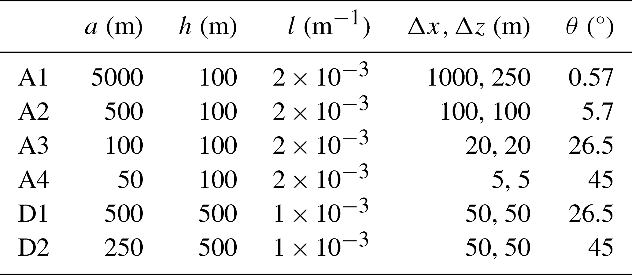
Figure 1 shows the simulated vertical velocity near the mountain. The results are similar to those of the three models in Satomura et al. (2003). In case A1 where al≫1, nearly hydrostatically balanced mountain waves appear, which propagate upward above the mountain. In case A2 where al≈1, nonhydrostatic mountain waves appear, which propagate upward and downstream relative to the mountain. In cases A3 and A4 where al≪1, wave structures diminish, and simple flow that climbs over and goes down the mountain is simulated (Satomura et al., 2003). In cases D1 and D2 where hl≪1, the mountain is high enough that nonlinear effects are taken into account (e.g., Smith, 1979; Satomura et al., 2003). In these cases, the amplitude of the vertical velocity is slightly larger than that derived from linear theory, which is probably because of nonlinear effects (Satomura et al., 2003; Li et al., 2016).

Figure 1 Simulated vertical velocity for cases (a) A1, (b) A2, (c) A3, (d) A4, (e) D1, and (f) D2. The contour intervals are 0.05, 0.1, 0.25, 1.0, 0.2, and 0.5 m s⁻¹, respectively.

Figure 2 Same as Fig. 1d, except for using ${\left[\mathrm{1}/m\cdot \partial \left(\mathit{\pi }\mathcal{P}\right)/\partial \mathit{\eta }\right]}_{\mathrm{s}}={\left[\mathrm{1}/m\cdot \partial \left(\mathit{\pi }\mathcal{P}\right)/\partial \mathit{\eta }\right]}_{\mathrm{3}/\mathrm{2}}$ for the surface boundary condition.

Figure 2 shows the result for case A4 when Eq. (21) is used instead of Eq. (18) for the surface boundary conditions. The result using Eq. (18) (Fig. 1d) is more similar to the model results and the linear theory in Satomura et al. (2003) than that using Eq. (21) (Fig. 2). Moreover, when Eq. (21) is used, the numerical stability is reduced, and the use of the GCR method with at least two iterations becomes necessary in case A4 for stable calculations. Therefore, the method using Eq. (18) is better than that using Eq. (21).

When $\widehat{d}$ is used instead of $\widehat{\widehat{d}}$, the numerical stability is decreased, and the use of the GCR method with at least two iterations becomes necessary in case A4.

When the no-recalculation method is used instead of the single-recalculation method, cases A4 and D2, which have an average mountain slope of 45°, become unstable, but cases A1–A3, and D1 remain stable. It is notable that even cases A3 and D1, which have an average mountain slope of 26.5°, remain stable with the no-recalculation method. When $\widehat{d}$ is used instead of $\widehat{\widehat{d}}$ in the no-recalculation method, cases A3, A4, D1, and D2 become unstable, indicating that the use of $\widehat{\widehat{d}}$ improves the numerical stability of the no-recalculation method.

When second-order decentering is not applied, that is, when β is reduced from 1.2 to 1.0, all six cases, A1–A4, D1, and D2, become unstable. For numerical stability in the constant-coefficient semi-implicit scheme, the constant-coefficient linear terms should be larger than the corresponding nonlinear terms in the original prognostic equations. Therefore, in Eq. (27) for v⁺, the coefficient $\mathit{\beta }\stackrel{\mathrm{‾}}{T}$ in the constant-coefficient linear term should be larger than the coefficient T of the corresponding nonlinear term. In Eq. (35) for ${\widehat{d}}^{+}$, the coefficient $\mathit{\beta }/\stackrel{\mathrm{‾}}{\stackrel{\mathrm{‾}}{T}}$ in the constant-coefficient linear term should also be larger than $\mathrm{1}/T$. From these conditions, $\stackrel{\mathrm{‾}}{\stackrel{\mathrm{‾}}{T}}/\mathit{\beta }<T<\mathit{\beta }\stackrel{\mathrm{‾}}{T}$ should be satisfied for the constant-coefficient semi-implicit scheme to provide sufficient stability. Reducing β from 1.2 to 1.0 narrows the temperature range satisfying this condition. Therefore, additional experiments were performed with β=1.0, $\stackrel{\mathrm{‾}}{T}=\mathrm{300}\times \mathrm{1.2}$ K, and $\stackrel{\mathrm{‾}}{\stackrel{\mathrm{‾}}{T}}=\mathrm{160}/\mathrm{1.2}$ K, which retains the original bounds of this temperature range. With this setting, cases A4, D1, and D2 become stable, but cases A1–A3 remain unstable. This result indicates that the above condition alone is not sufficient for numerical stability and that the effects of β>1.0 in Eq. (29) for lnT⁺, in Eq. (30) for 𝒬⁺, and in Eq. (31) for $\ln {\mathit{\pi }}_{\mathrm{s}}^{+}$ also contribute to numerical stability.

3.3 Extremely steep mountain test case

A case with an extremely steep mountain with an average slope of 63.4° (herein, case S1) was also simulated. Table 2 provides the simulation conditions for case S1, where h and l are the same as in case D2, and a is halved as compared with case D2. The number of vertical grids is K = 10 000$/\mathrm{\Delta }z$ and the sponge layer using Rayleigh damping is placed above 7500 m height. The integration time is set to 50 min and the timestep is set to 0.3 s. In case S1, the preconditioned GCR method with a maximum number of iterations N_{max_iter}=4 (Appendix E3) is used here for the semi-implicit calculation, because the single-recalculation method or the GCR method with N_{max_iter}<4 leads to numerical instability.

Table 2 Conditions for the extremely steep mountain test case.

Figure 3a shows the vertical velocity in case S1. After the wind passes over the mountain, a very strong downslope wind appears near the surface. Figure 3b shows the wind vectors (u,w) in case S1. The wind over the mountain splits into two parts: one that moves eastward and the other that descends near the surface. Figure 3c–d are the same as Fig. 3a–b, except that the initial condition for w is given by $w=\mathit{v}\cdot \mathrm{\nabla }\mathrm{\Phi }/g$ instead of w=0. A large rotor forms downwind of the mountain. Notably, two completely different states appear under identical conditions except for the initial conditions of w. When the previous vertical interpolation method is applied to compute vertical transport at the lowest and highest levels (Appendix B3), results similar to those in Fig. 3a–b are obtained for both initial conditions. Thus, the results of case S1 appear to be highly sensitive to both the initial conditions of w and the computing method applied near the surface.

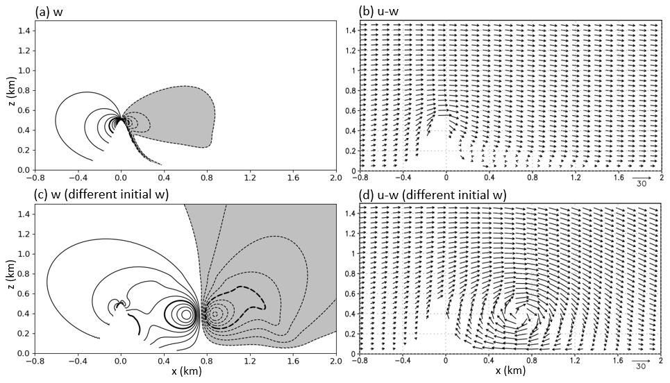
Figure 3 The results for case S1 with an extremely steep mountain. (a) Simulated vertical velocities (contour interval: 2.0 m s⁻¹) and (b) simulated wind vectors for $\mathrm{\Delta }x=\mathrm{\Delta }z=\mathrm{10}$ m, and Δt=0.3 s. Panels (c) and (d) are the same as (a) and (b), respectively, except that the initial condition for w is given by $w=\mathit{v}\cdot \mathrm{\nabla }\mathrm{\Phi }/g$ instead of w=0.

3.4 Mountain wave test cases of Schär et al. (2002)

Two mountain wave test cases of Schär et al. (2002) were performed, which are referred to as case Schär1 and case Schär2 in this paper. The surface height is given as

$$\begin{array}{}\text{(38)}& z_{\mathrm{s}}=h_{\mathrm{0}}\exp \left[-{\left({\displaystyle \frac{x}{a}}\right)}^{\mathrm{2}}\right]{\cos }^{\mathrm{2}}\left({\displaystyle \frac{\mathit{\pi }x}{\mathit{\lambda }}}\right),\end{array}$$

where h₀=250 m, a=5 km, and λ=4 km. Table 3 provides the simulation conditions of cases Schär1 and Schär2, where the Brunt–Väisälä frequency N, initial horizontal wind velocity U, Scorer parameter $l=N/U$, grid intervals Δx and Δz, upstream surface temperature T₀, and surface pressure p₀ are specified. The horizontal extent is L=200 km. The number of vertical levels is K=65, and Rayleigh damping is used above a height of 35Δz to minimize reflections. The integration time is 600 min.

Table 3 Conditions for the mountain wave test cases of Schär et al. (2002).

Figure 4 shows the results for case Schär1. Figure 4a–c show the vertical velocity when using timesteps of 5, 30, and 60 s, respectively. These results are similar to the analytical solution of Schär et al. (2002), even with long timesteps. In Schär et al. (2002), the results were good when using a smooth level vertical (SLEVE) coordinate, but not good when using the usual hybrid height coordinate. In our model, good results are obtained with the usual hybrid mass-based coordinate, possibly because of the use of the vertically conservative semi-Lagrangian scheme. Figure 4d–f are the same as Fig. 4a–c, except for not using the semi-Lagrangian treatment of the pressure change (SLTPC) that is explained in Appendix B7. The result with the long timestep of 60 s is not good when not using the SLTPC, which indicates that the SLTPC is effective when using a long timestep.

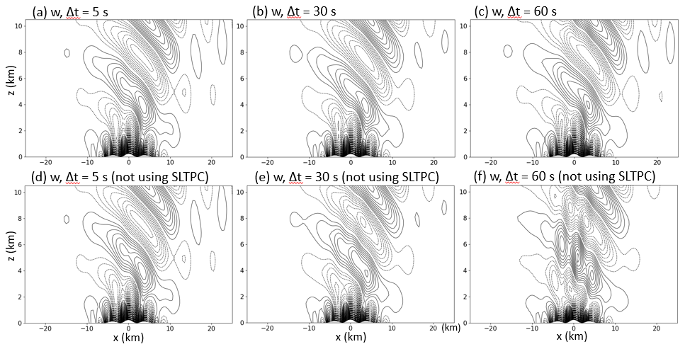
Figure 4 Simulated vertical velocity for case Schär1 using (a) Δt=5 s, (b) Δt=30 s, and (c) Δt=60 s. Panels (d)–(f) are the same as (a)–(c), respectively, except for not using the semi-Lagrangian treatment of the pressure change (SLTPC). The contour interval is 0.05 m s⁻¹.

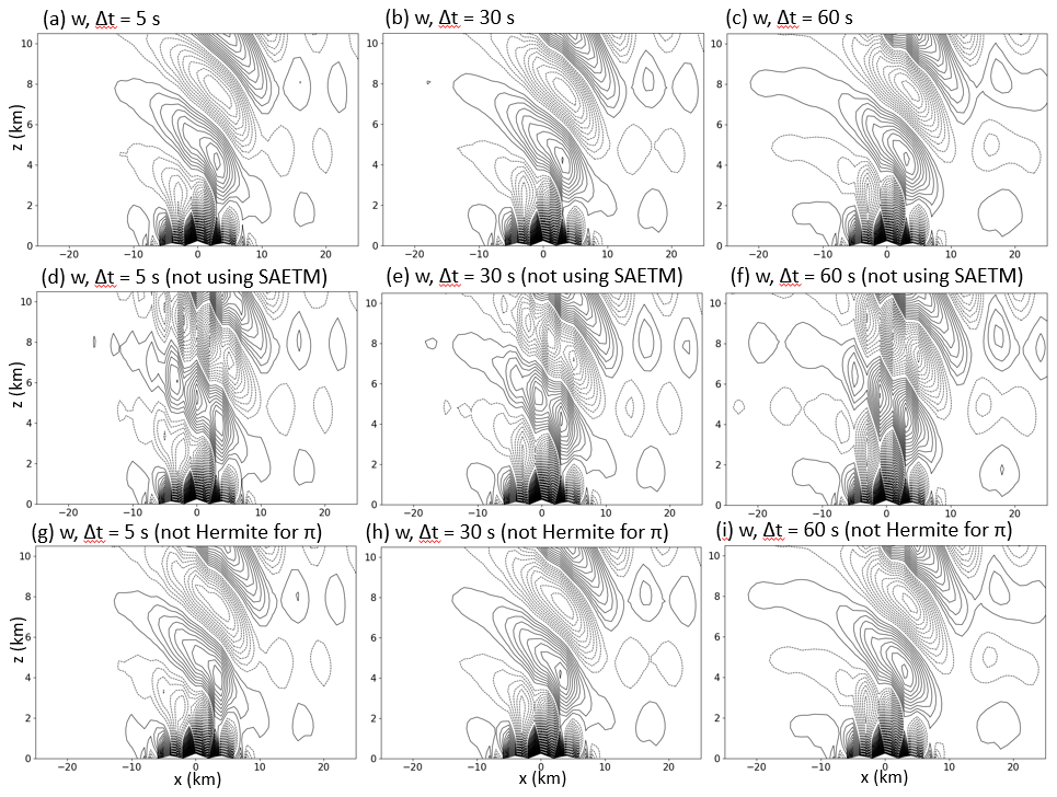
Figure 5 Simulated vertical velocity for case Schär2 using (a) Δt=5 s, (b) Δt=30 s, and (c) Δt=60 s. Panels (d)–(f) are the same as (a)–(c), respectively, except for not using the spatially averaged Eulerian treatment of the mountains (SAETM). Panels (g)–(i) are the same as (a)–(c), respectively, except for not using the cubic Hermite interpolation for the SLTPC. The contour interval is 0.09355 m s⁻¹.

Figure 5 shows the results for case Schär2. Figure 5a–c show the vertical velocity with timesteps of 5, 30, and 60 s, respectively, which are also similar to the analytical solution in Schär et al. (2002) even with long timesteps. Figure 5d–f are the same as Fig. 5a–c, except for not using the spatially averaged Eulerian treatment of mountains (SAETM; Appendix B6) for the horizontal mass advection, which yields poor results. Figure 5g–i are the same as Fig. 5a–c, except for not using the cubic Hermite interpolation (Appendix B8) and using the Lagrange interpolation for SLTPC. The result around $x=-\mathrm{5}$ km with a short timestep of Δt=5 s when not using the cubic Hermite interpolation (Fig. 5g) is not as good as that when using the interpolation (Fig. 5a).

3.5 Density current test case

The density current test case of Straka et al. (1993) was performed. The basic state values are given as follows:

$$\begin{array}{}\text{(39)}& {\displaystyle }\stackrel{\mathrm{‾}}{T}=T_{\mathrm{s}}-zg/c_{\mathrm{p}},\text{(39')}& {\displaystyle }\stackrel{\mathrm{‾}}{\mathit{\theta }}=T_{\mathrm{s}}=\mathrm{300}\mathrm{K}.\end{array}$$

To initiate a density current, the following function is used to specify an initial temperature perturbation:

$$\begin{array}{}\text{(40)}& \mathrm{\Delta }T=\left\{\begin{array}{ll}\mathrm{0.0}\mathit{°}\mathrm{C}& \mathrm{if}L>\mathrm{1.0},\\ -\mathrm{15.0}\left[\cos \left(\mathit{\pi }L\right)+\mathrm{1.0}\right]/\mathrm{2}\mathit{°}\mathrm{C}& \mathrm{if}L\le \mathrm{1.0},\end{array}\right.\end{array}$$

where $L={\left\{{\left[\left(x-x_{\mathrm{c}}\right)x_{\mathrm{r}}^{-\mathrm{1}}\right]}^{\mathrm{2}}+{\left[\left(z-z_{\mathrm{c}}\right)z_{\mathrm{r}}^{-\mathrm{1}}\right]}^{\mathrm{2}}\right\}}^{\mathrm{0.5}}$, x_c=0.0 km, x_r=4.0 km, z_c=3.0 km and z_r=2.0 km. The horizontal extent is from $x=-\mathrm{25.6}$ km to x=25.6 km, and the number of vertical grids is $K=\mathrm{6400}/\mathrm{\Delta }z$. Second-order x–z diffusion with a diffusion coefficient of 75.0 m² s⁻¹, as specified by Straka et al. (1993), is used for T, 𝒬, D, and $\widehat{\widehat{d}}$ in spectral space. In test cases without mountains, no recalculation of the non-constant coefficient linear terms L_N,v and $L_{\mathrm{N},\widehat{\widehat{d}}}$ is necessary to solve the semi-implicit equations without stability problems, because the values of L_N,v and $L_{\mathrm{N},\widehat{\widehat{d}}}$, which contain ∇Φ^#, are small (Appendix E1).

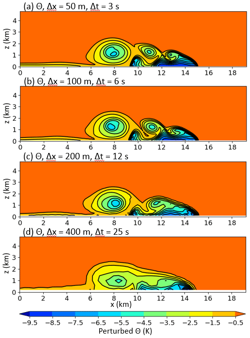
Figure 6 Simulated potential temperature perturbations (K) at 900 s in the density current test case of Straka et al. (1993). (a) $\mathrm{\Delta }x=\mathrm{\Delta }z=\mathrm{50}$ m and Δt=3 s. (b) $\mathrm{\Delta }x=\mathrm{\Delta }z=\mathrm{100}$ m and Δt=6 s. (c) $\mathrm{\Delta }x=\mathrm{\Delta }z=\mathrm{200}$ m and Δt=12 s. (d) $\mathrm{\Delta }x=\mathrm{\Delta }z=\mathrm{400}$ m and Δt=25 s.

Figure 6 shows the simulated potential temperature perturbations at 900 s. The result with $\mathrm{\Delta }x=\mathrm{\Delta }z=\mathrm{50}$ m and Δt=3 s (Fig. 6a) is similar to the result of the reference model (REFC) with $\mathrm{\Delta }x=\mathrm{\Delta }z=\mathrm{50}$ m and $\mathrm{\Delta }t=\mathrm{1.5625}\times {\mathrm{10}}^{-\mathrm{2}}$ s in Straka et al. (1993) despite the long timestep of 3 s. The result at low resolution with $\mathrm{\Delta }x=\mathrm{\Delta }z=\mathrm{400}$ m and Δt=25 s (Fig. 6d) is more similar to the result with $\mathrm{\Delta }x=\mathrm{\Delta }z=\mathrm{50}$ m, compared with the results of Straka et al. (1993) at the same resolution. This is probably because the model has good computational accuracy by using the spectral method and good numerical stability by using the semi-implicit semi-Lagrangian scheme.

3.6 Warm bubble convection test case

The warm bubble convection test case of Robert (1993) was simulated. The basic state of the atmosphere is isentropic with a potential temperature of 30 °C. The initial perturbation of the potential temperature within the bubble is given by

$$\begin{array}{}\text{(41)}& {\mathit{\theta }}^{\prime }=\left\{\begin{array}{ll}A,& r\le a\\ A\exp \left[-{\left(r-a\right)}^{\mathrm{2}}/s^{\mathrm{2}}\right],& r>a,\end{array}\right.\end{array}$$

with

$$\begin{array}{}\text{(42)}& r^{\mathrm{2}}={\left(x-x_{\mathrm{0}}\right)}^{\mathrm{2}}+{\left(z-z_{\mathrm{0}}\right)}^{\mathrm{2}},\end{array}$$

where A=0.5 °C, a=50 m, s=100 m, x₀=500 m, and z₀=260 m. This produces a bubble with a Gaussian profile with a small flat region at its center. The grid intervals are Δx=10 m and Δz=10 m, the horizontal length of the domain is L=1 km, and the number of vertical grids is $K=\mathrm{1500}/\mathrm{\Delta }z$.

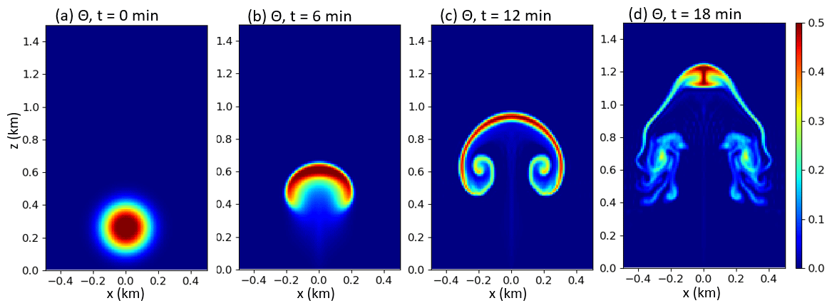
Figure 7 Simulated potential temperature perturbations (K) at (a) t=0min, (b) t=6 min, (c) t=12 min, and (d) t=18 min in the warm bubble convection test case of Robert (1993).

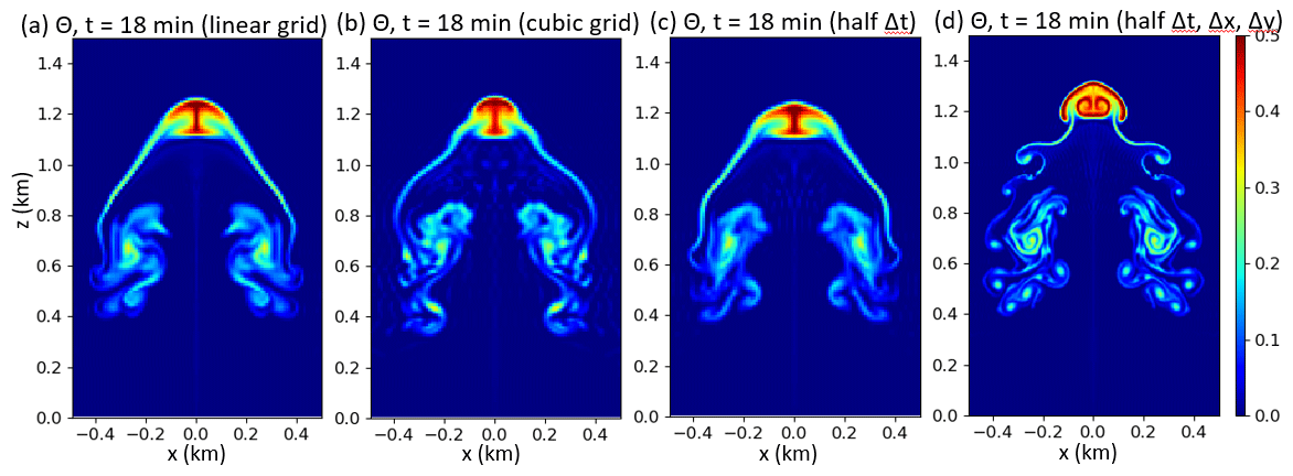
Figure 8 (a) Same as Fig. 7d, except for using linear truncation instead of quadratic truncation. (b) Same as Fig. 7d, except for using cubic truncation. (c) Same as Fig. 7d, except that Δt=2.5 s instead of Δt=5 s. (d) Same as (c), except that $\mathrm{\Delta }x=\mathrm{\Delta }z=\mathrm{5}$ m instead of $\mathrm{\Delta }x=\mathrm{\Delta }z=\mathrm{10}$ m.

Figure 7a–d show the potential temperature perturbations at t=0, 6, 12, and 18 min, respectively. The results at t=0, 6, and 12 min are very similar to those of Robert (1993). The result at t=18 min is similar to that of Robert (1993), but there are some differences. Figure 8a–d show the results at t=18 min with different settings. Figure 8a and b are the same as Fig. 7d, except for using the linear truncation $\left(M\cong I/\mathrm{2}-\mathrm{1}\right)$ and the cubic truncation $\left(M\cong I/\mathrm{4}\right)$, respectively, instead of the quadratic truncation $\left(M\cong I/\mathrm{3}\right)$. There are also some differences among their results. Figure 8c is the same as Fig. 7d, except for using Δt=2.5 s instead of Δt=5 s; these two results are similar. Figure 8d is the same as Fig. 8c, except for using Δx=5 m and Δz=5 m; small-scale sharp structures appear due to the higher resolution.

3.7 Gravity wave test case

The gravity wave test case of Skamarock and Klemp (1994) was simulated. The initial perturbation of potential temperature θ^′ is given as follows:

$$\begin{array}{}\text{(43)}& {\mathit{\theta }}^{\prime }=\mathrm{\Delta }{\mathit{\theta }}_{\mathrm{0}}{\displaystyle \frac{\sin \left(\frac{\mathit{\pi }z}{H}\right)}{\mathrm{1}+\frac{{\left(x-x_{\mathrm{c}}\right)}^{\mathrm{2}}}{a^{\mathrm{2}}}}},\end{array}$$

where $\mathrm{\Delta }{\mathit{\theta }}_{\mathrm{0}}={\mathrm{10}}^{-\mathrm{2}}$ K, a=5 km, the height of the domain H=10km, the horizontal length of the domain L=300 km, and the central position of the initial perturbation $x_{\mathrm{c}}=L/\mathrm{3}$. A constant Brunt–Väisälä frequency $N={\mathrm{10}}^{-\mathrm{2}}$ s⁻¹ and a surface temperature of 300 K give the basic state of the vertical temperature profile. The initial horizontal wind velocity is U=20 m s⁻¹. The grid intervals are $\mathrm{\Delta }x=\mathrm{\Delta }z=\mathrm{500}$ m.

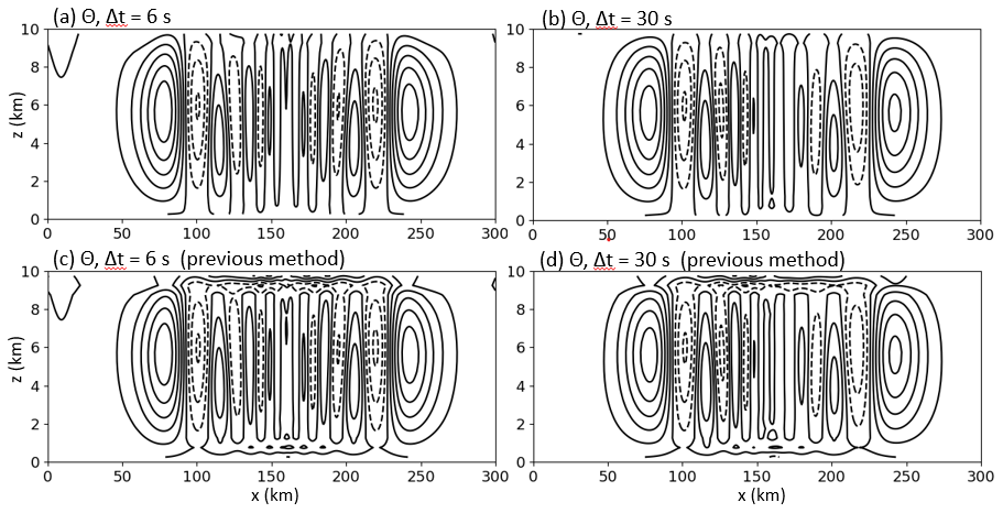
Figure 9 Simulated potential temperature perturbations at t=3000 s using (a) Δt=6 s and (b) Δt=30 s in the gravity wave test case of Skamarock and Klemp (1994). Panels (c) and (d) are the same as (a) and (b), respectively, except for using the previous method for vertical interpolation (Appendix B3). The contour interval is 0.0005 K.

Figure 9a–b show the potential temperature perturbations at t=3000 s using the timesteps Δt=6 s and Δt=30 s, respectively. The results are similar to those of Wong et al. (2014). Figure 9c–d show the results using the previous method of vertical interpolation for the vertical transport in the lowest and highest vertical levels (Appendix B3). The present method (Fig. 9a–b) improves the results as compared with the previous method.

4 Conclusions

We have developed a two-dimensional x–z nonhydrostatic spectral model using non-constant coefficient semi-implicit and vertically conservative semi-Lagrangian schemes to allow long timesteps. The model was examined using various test cases and good results were obtained with long timesteps and even with steep orography, because of the following features, including several improvements:

• Feature 1: The non-constant coefficient semi-implicit scheme is numerically stable and computationally efficient. A single recalculation of non-constant coefficient linear terms (i.e., the single-recalculation method; Appendix E2) is usually sufficient to solve the equations associated with the non-constant coefficient semi-implicit scheme with the help of Features 2–5, even for cases A4 and D2, which have a steep mountain with an average slope of 45° (Sect. 3.2). In case S1, which has an extremely steep mountain with an average slope of 63.4° (Sect. 3.3), several iterations using the preconditioned GCR method (Appendix E3) are necessary to solve the semi-implicit equations, where only non-constant coefficient linear terms are recalculated in each iteration. In the test cases without mountains (Sect. 3.5–3.7) and even in cases A3 and D1, which have a mountain with an average slope of 26.5° (Sect. 3.2), the no-recalculation method (Appendix E1) is sufficient to solve the semi-implicit equations.

• Feature 2: The combination of SETTLS and second-order decentering with β>1 (Sect. 2.4) improves numerical stability (Sect. 3.2).

• Feature 3: In the single-recalculation method, setting α^r=0.8 instead of α^r=1.0 improves the numerical stability (Appendix E2; Sect. 3.2).

• Feature 4: By improving the treatment of the free-slip boundary conditions, the number of iterations for solving the semi-implicit equations is reduced (Sect. 2.3), and the results for the test cases with a steep mountain are improved (Sect. 3.2).

• Feature 5: By using $\widehat{\widehat{d}}$, 𝒬 (Bénard et al., 2010), and lnT instead of $\widehat{d}$, 𝒫, and T as prognostic variables in spectral space, the numerical stability is improved, and the number of iterations needed to solve the semi-implicit equations is reduced (Sects. 2.5 and 3.2).

• Feature 6: A vertically conservative semi-Lagrangian scheme is used, where a conservative semi-Lagrangian method is used in the vertical direction (Appendix B). Mass and other variables are advected in a consistent manner.

• Feature 7: By using a spatially averaged Eulerian treatment of mountains with horizontal mass advection similar to Ritchie and Tanguay (1996) (Appendix B6), the results for the test cases with mountains are improved (Sect. 3.4).

• Feature 8: By treating the hydrostatic pressure change with horizontal advection in a semi-Lagrangian fashion (Appendix B7), the results for the test cases with mountains are improved (Sect. 3.4).

• Feature 9: By using cubic Hermite interpolation to calculate the hydrostatic pressure change with horizontal advection (Appendix B8), the results for case Schär2 with mountains are slightly improved when the timestep is short (Sect. 3.4).

• Feature 10: By modifying the vertical interpolation method for the vertical transport in the lowest and highest vertical levels (Appendix B3), the results for the gravity wave test case are improved (Sect. 3.7).

We have been developing a global nonhydrostatic spectral model using non-constant coefficient semi-implicit and vertically conservative semi-Lagrangian schemes, as briefly described by Yoshimura (2012). However, the improvements described in Features 3–5, 7, 9, and 10 above have not been implemented in the global model. These improvements will be implemented and evaluated in future work. Although we expect that these improvements can be incorporated into the global model without substantial difficulties, their performance, particularly that of the improved surface boundary treatment, should be evaluated in the three-dimensional global model. Further improvements will be made if necessary. Similar to the two-dimensional x–z nonhydrostatic model, the global nonhydrostatic model is expected to be computationally efficient: its expected high numerical stability would allow long timesteps, and the single-recalculation method is expected to be sufficient for stable time integration over realistic orography without extremely steep mountains, such as the mountain with a 63.4° slope, although this expectation should be confirmed in the global model. Furthermore, not only in this model but also in other nonhydrostatic models, introducing some improvements described in this paper is likely to enhance numerical stability, computational efficiency, and accuracy, particularly in cases with steep mountains.

Appendix A: How to obtain the coefficients $A_{k-\mathrm{1}/\mathrm{2}}$ and $B_{k-\mathrm{1}/\mathrm{2}}$ in the vertical coordinate of the two-dimensional x–z model

In the two-dimensional x–z model, $A_{k-\mathrm{1}/\mathrm{2}}$ and $B_{k-\mathrm{1}/\mathrm{2}}$ in Eq. (2) are defined as follows:

$$\begin{array}{}\text{(A1a)}& {\displaystyle }{A}_{k-\mathrm{1}/\mathrm{2}}\equiv {\mathit{\mu }}_{k-\mathrm{1}/\mathrm{2}}\times {\mathrm{10}}^{\mathrm{5}}\cdot {\mathit{\eta }}_{k-\mathrm{1}/\mathrm{2}},\text{(A1b)}& {\displaystyle }{B}_{k-\mathrm{1}/\mathrm{2}}\equiv \left(\mathrm{1}-{\mathit{\mu }}_{k-\mathrm{1}/\mathrm{2}}\right)\cdot {\mathit{\eta }}_{k-\mathrm{1}/\mathrm{2}},\text{(A1c)}& {\displaystyle }{\mathit{\mu }}_{k-\mathrm{1}/\mathrm{2}}\equiv \left\{\begin{array}{l}\mathrm{0}\mathrm{for}{\mathit{\gamma }}_{k-\mathrm{1}/\mathrm{2}}\le \mathrm{0},\\ {\mathit{\gamma }}_{k-\mathrm{1}/\mathrm{2}}+\mathrm{0.125}[-\mathrm{16}{\left({\mathit{\gamma }}_{k-\mathrm{1}/\mathrm{2}}-\mathrm{0.5}\right)}^{\mathrm{5}}\\ +{\mathit{\gamma }}_{k-\mathrm{1}/\mathrm{2}}-\mathrm{0.5}]\\ \mathrm{for}\mathrm{0}\le {\mathit{\gamma }}_{k-\mathrm{1}/\mathrm{2}}\le \mathrm{1},\\ \mathrm{1}\mathrm{for}{\mathit{\gamma }}_{k-\mathrm{1}/\mathrm{2}}\ge \mathrm{1},\end{array}\right.\text{(A1d)}& {\displaystyle }{\mathit{\gamma }}_{k-\mathrm{1}/\mathrm{2}}\equiv {\displaystyle \frac{\ln {\mathit{\eta }}_{\left[\mathrm{2}\right]}-\ln {\mathit{\eta }}_{k-\mathrm{1}/\mathrm{2}}}{\ln {\mathit{\eta }}_{\left[\mathrm{2}\right]}-\ln {\mathit{\eta }}_{\left[\mathrm{1}\right]}}},{\mathit{\eta }}_{\left[\mathrm{1}\right]}=\mathrm{0.1},{\mathit{\eta }}_{\left[\mathrm{2}\right]}=\mathrm{1.0}.\end{array}$$

When π_s=10⁵Pa, Eq. (2) becomes ${\mathit{\pi }}_{k-\mathrm{1}/\mathrm{2}}={\mathrm{10}}^{\mathrm{5}}\cdot {\mathit{\eta }}_{k-\mathrm{1}/\mathrm{2}}$. The vertical profile of ${\mathit{\eta }}_{k-\mathrm{1}/\mathrm{2}}$ is given by the following equations:

$$\begin{array}{}\text{(A2a)}& {\displaystyle }{\mathit{\eta }}_{\mathrm{1}/\mathrm{2}}=\mathrm{1}\left(\log {\mathit{\eta }}_{\mathrm{1}/\mathrm{2}}=\mathrm{0}\right),\text{(A2b)}& {\displaystyle }\log {\mathit{\eta }}_{k+\mathrm{1}/\mathrm{2}}=\log {\mathit{\eta }}_{k-\mathrm{1}/\mathrm{2}}-{\displaystyle \frac{g\mathrm{\Delta }z}{R{T}_k}},\left(\mathrm{1}\le k\le K-\mathrm{1}\right),\text{(A2c)}& {\displaystyle }{\mathit{\eta }}_{K+\mathrm{1}/\mathrm{2}}=\mathrm{0},\end{array}$$

where Δz is the vertical resolution. As an exception, in the gravity wave test case in Sect. 3.7, η_[1]=0.5 is used in Eq. (A1d), and ${\mathit{\eta }}_{K+\mathrm{1}/\mathrm{2}}$ is given using Eq. (A2b) instead of Eq. (A2c).

The vertical profiles of T_k in Eq. (A2b) are calculated as shown below. When the Brunt–Väisälä frequency N is given, the following relationship is satisfied:

$$\begin{array}{}\text{(A3)}& {\displaystyle \frac{\mathrm{d}T}{\mathrm{d}z}}={\displaystyle \frac{N^{\mathrm{2}}}{g}}T-{\displaystyle \frac{g}{c_{\mathrm{p}}}}.\end{array}$$

Equation (A3) is discretized vertically as follows:

$$\begin{array}{}\text{(A4)}& {\displaystyle \frac{T_{k+\mathrm{1}/\mathrm{2}}-T_{k-\mathrm{1}/\mathrm{2}}}{\mathrm{\Delta }z}}={\displaystyle \frac{N^{\mathrm{2}}}{g}}{\displaystyle \frac{T_{k+\mathrm{1}/\mathrm{2}}+T_{k-\mathrm{1}/\mathrm{2}}}{\mathrm{2}}}-{\displaystyle \frac{g}{c_{\mathrm{p}}}},\end{array}$$

which leads to:

$$\begin{array}{}\text{(A5)}& T_{k+\mathrm{1}/\mathrm{2}}={\displaystyle \frac{\left(\mathrm{1}+\frac{N^{\mathrm{2}}\mathrm{\Delta }z}{\mathrm{2}g}\right)T_{k-\mathrm{1}/\mathrm{2}}-\frac{g\mathrm{\Delta }z}{c_{\mathrm{p}}}}{\mathrm{1}-\frac{N^{\mathrm{2}}\mathrm{\Delta }z}{\mathrm{2}g}}}.\end{array}$$

When the surface temperature $T_{\mathrm{1}/\mathrm{2}}$ is given, $T_{k+\mathrm{1}/\mathrm{2}}\left(k=\mathrm{1},\mathrm{\dots },K-\mathrm{1}\right)$ is calculated using Eq. (A5), and T_k in Eq. (A2b) is given by:

$$\begin{array}{}\text{(A6)}& T_k={\displaystyle \frac{T_{k-\mathrm{1}/\mathrm{2}}+T_{k+\mathrm{1}/\mathrm{2}}}{\mathrm{2}}}\left(\mathrm{1}\le k\le K-\mathrm{1}\right).\end{array}$$

Appendix B: Vertically conservative semi-Lagrangian scheme

A simple explanation of the vertically conservative semi-Lagrangian scheme was given by Yoshimura and Matsumura (2003) and Yukimoto et al. (2011). The scheme has some similarities to the vertically Lagrangian scheme of Lin (2004). Here, the scheme is described in detail, including some improvements.

In the vertically conservative semi-Lagrangian scheme, the three-dimensional model is regarded as a vertical stack of two-dimensional horizontal models, and horizontal advection is calculated separately in each layer. Conservative vertical remapping is performed before and after horizontal advection to maintain consistency with the layers defined by the η coordinate. This vertical remapping corresponds to vertical transport of mass. Mass and other variables are advected in a consistent manner.

The effects of horizontal divergence and vertical remapping are calculated with equal weighting before and after horizontal advection. This treatment is consistent with the semi-Lagrangian time discretization, where the tendencies at the departure and arrival points are taken into account with equal weighting. This symmetric treatment is designed to preserve second-order temporal accuracy along the semi-Lagrangian trajectory. Although the splitting between horizontal and vertical transport introduces an additional splitting error, the weak dependence on the timestep size in the test cases examined here suggests that the splitting error is small.

Appendix B1 describes a usual semi-Lagrangian scheme, Appendix B2 describes the vertically conservative semi-Lagrangian scheme, Appendix B3 describes vertical remapping, Appendices B4 and B5 describe horizontal advection, and Appendices B6–B8 describe several improvements related to horizontal advection.

B1 Advection with a usual semi-Lagrangian scheme

The advection equation with variable T can be expressed as follows:

$$\begin{array}{}\text{(B1)}& {\displaystyle \frac{\mathrm{d}T}{\mathrm{d}t}}\left(={\displaystyle \frac{\partial T}{\partial t}}+\mathit{v}\cdot \mathrm{\nabla }T+\dot{\mathit{\eta }}{\displaystyle \frac{\partial T}{\partial \mathit{\eta }}}\right)=\mathrm{0}.\end{array}$$

In the usual non-conservative semi-Lagrangian scheme (e.g., Robert, 1981; Temperton et al., 2001; Hortal, 2002), Eq. (B1) is discretized in time as

$$\begin{array}{}\text{(B2)}& {\displaystyle \frac{T^{+}-T_{\mathrm{D}}^{\mathrm{0}}}{\mathrm{\Delta }t}}=\mathrm{0},\end{array}$$

where the subscript D represents the value at the three-dimensional departure point x_D and the absence of the subscript D means the value at the arrival point x, which is on the grid point. The departure point x_D is located upstream from the arrival point x along the wind vector. Equation (B2) is the discretization when the right side of Eq. (B1) is zero. Section 2.4 and 2.5 show the discretization when the right side of Eq. (B1) is not zero.

B2 Advection of mass and other variables with the vertically conservative semi-Lagrangian scheme

In the vertically conservative semi-Lagrangian scheme, the value $T^{+}\left(=T_{\mathrm{D}}^{\mathrm{0}}\right)$ in Eq. (B2) is obtained by calculating horizontal and vertical transport separately. A conservative semi-Lagrangian scheme is used in the vertical direction. The continuous equation in Eq. (11) is converted to

$$\begin{array}{}\text{(B3)}& {\displaystyle \frac{{\mathrm{d}}_{\mathrm{H}}}{\mathrm{d}t}}\left({\displaystyle \frac{\partial \mathit{\pi }}{\partial \mathit{\eta }}}\right)=-D{\displaystyle \frac{\partial \mathit{\pi }}{\partial \mathit{\eta }}}-{\displaystyle \frac{\partial }{\partial \mathit{\eta }}}\left(\dot{\mathit{\eta }}{\displaystyle \frac{\partial \mathit{\pi }}{\partial \mathit{\eta }}}\right),\end{array}$$

where D is the horizontal divergence and ${\mathrm{d}}_{\mathrm{H}}/\mathrm{d}t\equiv \partial /\partial t+\mathit{v}\cdot \mathrm{\nabla }$ is the horizontal advection. Using Eq. (B3), Eq. (B1) is converted into:

$$\begin{array}{}\text{(B4)}& {\displaystyle \frac{{\mathrm{d}}_{\mathrm{H}}}{\mathrm{d}t}}\left({\displaystyle \frac{\partial \mathit{\pi }}{\partial \mathit{\eta }}}T\right)=-D{\displaystyle \frac{\partial \mathit{\pi }}{\partial \mathit{\eta }}}T-{\displaystyle \frac{\partial }{\partial \mathit{\eta }}}\left(\dot{\mathit{\eta }}{\displaystyle \frac{\partial \mathit{\pi }}{\partial \mathit{\eta }}}T\right).\end{array}$$

Using Eqs. (B3) and (B4), the mass and other variables are advected in a consistent manner. Using Eq. (3), Eqs. (B3) and (B4) are discretized in the vertical direction as follows:

$$\begin{array}{}\text{(B5)}& {\displaystyle }\begin{array}{rl}{\displaystyle \frac{{\mathrm{d}}_{\mathrm{H}}}{\mathrm{d}t}}\left(\mathrm{\Delta }{\mathit{\pi }}_k\right)& =-D_k\mathrm{\Delta }{\mathit{\pi }}_k-{\left(\dot{\mathit{\eta }}{\displaystyle \frac{\partial \mathit{\pi }}{\partial \mathit{\eta }}}\right)}_{k-\mathrm{1}/\mathrm{2}}\\ & +{\left(\dot{\mathit{\eta }}{\displaystyle \frac{\partial \mathit{\pi }}{\partial \mathit{\eta }}}\right)}_{k+\mathrm{1}/\mathrm{2}},\end{array}\text{(B6)}& {\displaystyle }\begin{array}{rl}{\displaystyle \frac{{\mathrm{d}}_{\mathrm{H}}}{\mathrm{d}t}}\left(\mathrm{\Delta }{\mathit{\pi }}_k{T}_k\right)& =-D_k\mathrm{\Delta }{\mathit{\pi }}_k{T}_k-{\left(\dot{\mathit{\eta }}{\displaystyle \frac{\partial \mathit{\pi }}{\partial \mathit{\eta }}}T\right)}_{k-\mathrm{1}/\mathrm{2}}\\ & +{\left(\dot{\mathit{\eta }}{\displaystyle \frac{\partial \mathit{\pi }}{\partial \mathit{\eta }}}T\right)}_{k+\mathrm{1}/\mathrm{2}}.\end{array}\end{array}$$

By using the SETTLS discretization, Eqs. (B5) and (B6) are discretized in time at each layer k as follows:

$$\begin{array}{}\text{(B7)}& {\displaystyle }\begin{array}{rl}\mathrm{\Delta }{\mathit{\pi }}_k^{+}& =\mathit{\{}\mathrm{\Delta }{\mathit{\pi }}_k^{\mathrm{0}}+{\displaystyle \frac{\mathrm{\Delta }t}{\mathrm{2}}}{\left(-D_k\mathrm{\Delta }{\mathit{\pi }}_k\right)}^{\left(+\right)}\\ & +{\displaystyle \frac{\mathrm{\Delta }t}{\mathrm{2}}}[-{\left(\dot{\mathit{\eta }}{\displaystyle \frac{\partial \mathit{\pi }}{\partial \mathit{\eta }}}\right)}_{k-\mathrm{1}/\mathrm{2}}^{\left(+\right)}+{\left(\dot{\mathit{\eta }}{\displaystyle \frac{\partial \mathit{\pi }}{\partial \mathit{\eta }}}\right)}_{k+\mathrm{1}/\mathrm{2}}^{\left(+\right)}]{\mathit{\}}}_{D_{\mathrm{2}}\left(k\right)}\\ & +{\displaystyle \frac{\mathrm{\Delta }t}{\mathrm{2}}}{\left(-D_k\mathrm{\Delta }{\mathit{\pi }}_k\right)}^{\mathrm{0}}\\ & +{\displaystyle \frac{\mathrm{\Delta }t}{\mathrm{2}}}\left[-{\left(\dot{\mathit{\eta }}{\displaystyle \frac{\partial \mathit{\pi }}{\partial \mathit{\eta }}}\right)}_{k-\mathrm{1}/\mathrm{2}}^{\mathrm{0}}+{\left(\dot{\mathit{\eta }}{\displaystyle \frac{\partial \mathit{\pi }}{\partial \mathit{\eta }}}\right)}_{k+\mathrm{1}/\mathrm{2}}^{\mathrm{0}}\right],\end{array}\text{(B8)}& {\displaystyle }\begin{array}{rl}\mathrm{\Delta }{\mathit{\pi }}_k^{+}{T}_k^{+}& =\mathit{\{}\mathrm{\Delta }{\mathit{\pi }}_k^{\mathrm{0}}{T}_k^{\mathrm{0}}+{\displaystyle \frac{\mathrm{\Delta }t}{\mathrm{2}}}{\left(-D_k\mathrm{\Delta }{\mathit{\pi }}_k\right)}^{\left(+\right)}{T}_k^{\mathrm{0}}\\ & +{\displaystyle \frac{\mathrm{\Delta }t}{\mathrm{2}}}[-{\left(\dot{\mathit{\eta }}{\displaystyle \frac{\partial \mathit{\pi }}{\partial \mathit{\eta }}}T\right)}_{k-\mathrm{1}/\mathrm{2}}^{\left(+\right)}+{\left(\dot{\mathit{\eta }}{\displaystyle \frac{\partial \mathit{\pi }}{\partial \mathit{\eta }}}T\right)}_{k+\mathrm{1}/\mathrm{2}}^{\left(+\right)}]{\mathit{\}}}_{D_{\mathrm{2}}\left(k\right)}\\ & +{\displaystyle \frac{\mathrm{\Delta }t}{\mathrm{2}}}{\left(-D_k\mathrm{\Delta }{\mathit{\pi }}_k\right)}^{\mathrm{0}}{T}_k^{+}\\ & +{\displaystyle \frac{\mathrm{\Delta }t}{\mathrm{2}}}\left[-{\left(\dot{\mathit{\eta }}{\displaystyle \frac{\partial \mathit{\pi }}{\partial \mathit{\eta }}}T\right)}_{k-\mathrm{1}/\mathrm{2}}^{\mathrm{0}}+{\left(\dot{\mathit{\eta }}{\displaystyle \frac{\partial \mathit{\pi }}{\partial \mathit{\eta }}}T\right)}_{k+\mathrm{1}/\mathrm{2}}^{\mathrm{0}}\right],\end{array}\end{array}$$

where the subscript D₂(k) indicates the value at the two-dimensional horizontal departure point in the vertical level k, and the absence of the subscript D₂(k) indicates the value at the arrival point.

Time integration of Eqs. (B7) and (B8) is performed in the following order:

Step 1: Initial values to be advected are

$$\begin{array}{}\text{(B9)}& {\displaystyle }\mathrm{\Delta }{\mathit{\pi }}_k\left[\mathrm{1}\right]=\mathrm{\Delta }{\mathit{\pi }}_k^{\mathrm{0}},\text{(B10)}& {\displaystyle }{T}_k\left[\mathrm{1}\right]=T_k^{\mathrm{0}}.\end{array}$$

Step 2: Due to horizontal divergence, the values of Δπ_k and T_k change as follows:

$$\begin{array}{}\text{(B11)}& {\displaystyle }\mathrm{\Delta }{\mathit{\pi }}_k\left[\mathrm{2}\right]=\mathrm{\Delta }{\mathit{\pi }}_k\left[\mathrm{1}\right]+{\displaystyle \frac{\mathrm{\Delta }t}{\mathrm{2}}}{\left(-D_k\mathrm{\Delta }{\mathit{\pi }}_k\right)}^{\left(+\right)},\text{(B12)}& {\displaystyle }\begin{array}{rl}\mathrm{\Delta }{\mathit{\pi }}_k\left[\mathrm{2}\right]T_k\left[\mathrm{2}\right]& =\mathrm{\Delta }{\mathit{\pi }}_k\left[\mathrm{1}\right]T_k\left[\mathrm{1}\right]\\ & +{\displaystyle \frac{\mathrm{\Delta }t}{\mathrm{2}}}{\left(-D_k\mathrm{\Delta }{\mathit{\pi }}_k\right)}^{\left(+\right)}{T}_k\left[\mathrm{1}\right].\end{array}\end{array}$$

From Eqs. (B11) and (B12),

$$\begin{array}{}\text{(B13)}& T_k\left[\mathrm{2}\right]=T_k\left[\mathrm{1}\right].\end{array}$$

Step 3: Due to the vertical flux, the values of Δπ_k and T_k change as follows:

$$\begin{array}{}\text{(B14)}& {\displaystyle }\begin{array}{rl}\mathrm{\Delta }{\mathit{\pi }}_k\left[\mathrm{3}\right]& =\mathrm{\Delta }{\mathit{\pi }}_k\left[\mathrm{2}\right]+{\displaystyle \frac{\mathrm{\Delta }t}{\mathrm{2}}}[-{\left(\dot{\mathit{\eta }}{\displaystyle \frac{\partial \mathit{\pi }}{\partial \mathit{\eta }}}\right)}_{k-\mathrm{1}/\mathrm{2}}^{\left(+\right)}\\ & +{\left(\dot{\mathit{\eta }}{\displaystyle \frac{\partial \mathit{\pi }}{\partial \mathit{\eta }}}\right)}_{k+\mathrm{1}/\mathrm{2}}^{\left(+\right)}],\end{array}\text{(B15)}& {\displaystyle }\begin{array}{rl}\mathrm{\Delta }{\mathit{\pi }}_k\left[\mathrm{3}\right]T_k\left[\mathrm{3}\right]& =\mathrm{\Delta }{\mathit{\pi }}_k\left[\mathrm{2}\right]T_k\left[\mathrm{2}\right]+{\displaystyle \frac{\mathrm{\Delta }t}{\mathrm{2}}}[-{\left(\dot{\mathit{\eta }}{\displaystyle \frac{\partial \mathit{\pi }}{\partial \mathit{\eta }}}T\right)}_{k-\mathrm{1}/\mathrm{2}}^{\left(+\right)}\\ & +{\left(\dot{\mathit{\eta }}{\displaystyle \frac{\partial \mathit{\pi }}{\partial \mathit{\eta }}}T\right)}_{k+\mathrm{1}/\mathrm{2}}^{\left(+\right)}].\end{array}\end{array}$$

Here, ${\left(\dot{\mathit{\eta }}\partial \mathit{\pi }/\partial \mathit{\eta }\right)}_{k-\mathrm{1}/\mathrm{2}}$ is calculated from the following equation (e.g., Ritchie et al., 1995):

$$\begin{array}{}\text{(B16)}& \begin{array}{rl}{\left(\dot{\mathit{\eta }}{\displaystyle \frac{\partial \mathit{\pi }}{\partial \mathit{\eta }}}\right)}_{k-\mathrm{1}/\mathrm{2}}& =B_{k-\mathrm{1}/\mathrm{2}}\sum _{j=\mathrm{1}}^K\left[D_j\mathrm{\Delta }{\mathit{\pi }}_j+{\mathit{\pi }}_{\mathrm{s}}\left({\mathit{v}}_j\cdot \mathrm{\nabla }\ln {\mathit{\pi }}_{\mathrm{s}}\right)\mathrm{\Delta }{B}_j\right]\\ & -\sum _{j=k}^K\left[D_j\mathrm{\Delta }{\mathit{\pi }}_j+{\mathit{\pi }}_{\mathrm{s}}\left({\mathit{v}}_j\cdot \mathrm{\nabla }\ln {\mathit{\pi }}_{\mathrm{s}}\right)\mathrm{\Delta }{B}_j\right],\end{array}\end{array}$$

where ${\left(\dot{\mathit{\eta }}\partial \mathit{\pi }/\partial \mathit{\eta }\right)}_{\mathrm{1}/\mathrm{2}}={\left(\dot{\mathit{\eta }}\partial \mathit{\pi }/\partial \mathit{\eta }\right)}_{K+\mathrm{1}/\mathrm{2}}=\mathrm{0}$. The value T_k[3] is calculated from T_k[2] using Eq. (B15) via the remapping method described in Appendix B3.

Step 4: Due to horizontal advection, the values of Δπ_k and T_k change as follows:

$$\begin{array}{}\text{(B17)}& {\displaystyle }\mathrm{\Delta }{\mathit{\pi }}_k\left[\mathrm{4}\right]={\left(\mathrm{\Delta }{\mathit{\pi }}_k\left[\mathrm{3}\right]\right)}_{D_{\mathrm{2}}\left(k\right)},\text{(B18)}& {\displaystyle }\mathrm{\Delta }{\mathit{\pi }}_k\left[\mathrm{4}\right]T_k\left[\mathrm{4}\right]={\left(\mathrm{\Delta }{\mathit{\pi }}_k\left[\mathrm{3}\right]\right)}_{D_{\mathrm{2}}}{\left(T_k\left[\mathrm{3}\right]\right)}_{D_{\mathrm{2}}\left(k\right)}.\end{array}$$

When adopting the spatially averaged Eulerian treatment of the mountains described in Appendix B6, Eq. (B44) below is used instead of Eq. (B17). From Eqs. (B17) and (B18),

$$\begin{array}{}\text{(B19)}& T_k\left[\mathrm{4}\right]={\left(T_k\left[\mathrm{3}\right]\right)}_{D_{\mathrm{2}}\left(k\right)}.\end{array}$$

How to calculate the horizontal departure point and the value at the horizontal departure point with the subscript D₂(k) is explained in Appendix B4.

Step 5: Due to the vertical flux, the values of Δπ_k and T_k change as follows:

$$\begin{array}{}\text{(B20)}& {\displaystyle }\begin{array}{rl}\mathrm{\Delta }{\mathit{\pi }}_k\left[\mathrm{5}\right]& =\mathrm{\Delta }{\mathit{\pi }}_k\left[\mathrm{4}\right]+{\displaystyle \frac{\mathrm{\Delta }t}{\mathrm{2}}}[-{\left(\dot{\mathit{\eta }}{\displaystyle \frac{\partial \mathit{\pi }}{\partial \mathit{\eta }}}\right)}_{k-\mathrm{1}/\mathrm{2}}^{\mathrm{0}}\\ & +{\left(\dot{\mathit{\eta }}{\displaystyle \frac{\partial \mathit{\pi }}{\partial \mathit{\eta }}}\right)}_{k+\mathrm{1}/\mathrm{2}}^{\mathrm{0}}],\end{array}\text{(B21)}& {\displaystyle }\begin{array}{rl}\mathrm{\Delta }{\mathit{\pi }}_k\left[\mathrm{5}\right]T_k\left[\mathrm{5}\right]& =\mathrm{\Delta }{\mathit{\pi }}_k\left[\mathrm{4}\right]T_k\left[\mathrm{4}\right]+{\displaystyle \frac{\mathrm{\Delta }t}{\mathrm{2}}}[-{\left(\dot{\mathit{\eta }}{\displaystyle \frac{\partial \mathit{\pi }}{\partial \mathit{\eta }}}T\right)}_{k-\mathrm{1}/\mathrm{2}}^{\mathrm{0}}\\ & +{\left(\dot{\mathit{\eta }}{\displaystyle \frac{\partial \mathit{\pi }}{\partial \mathit{\eta }}}T\right)}_{k+\mathrm{1}/\mathrm{2}}^{\mathrm{0}}].\end{array}\end{array}$$

Here, ${\left(\dot{\mathit{\eta }}\partial \mathit{\pi }/\partial \mathit{\eta }\right)}_{k-\mathrm{1}/\mathrm{2}}$ calculated from Eq. (B16) is not used, and Δπ_k[5] is calculated from Eq. (B29) below so that Eq. (B28) below is satisfied. After calculating Δπ_k[5], T_k[5] is calculated from T_k[4] using Eq. (B21) by the remapping method described in Appendix B3.

Step 6: Due to horizontal divergence, the values of Δπ_k and T_k change as follows:

$$\begin{array}{}\text{(B22)}& {\displaystyle }\mathrm{\Delta }{\mathit{\pi }}_k\left[\mathrm{6}\right]=\mathrm{\Delta }{\mathit{\pi }}_k\left[\mathrm{5}\right]+{\displaystyle \frac{\mathrm{\Delta }t}{\mathrm{2}}}{\left(-D_k\mathrm{\Delta }{\mathit{\pi }}_k\right)}^{\mathrm{0}},\text{(B23)}& {\displaystyle }\begin{array}{rl}\mathrm{\Delta }{\mathit{\pi }}_k\left[\mathrm{6}\right]T_k\left[\mathrm{6}\right]& =\mathrm{\Delta }{\mathit{\pi }}_k\left[\mathrm{5}\right]T_k\left[\mathrm{5}\right]\\ & +{\displaystyle \frac{\mathrm{\Delta }t}{\mathrm{2}}}{\left(-D_k\mathrm{\Delta }{\mathit{\pi }}_k\right)}^{\mathrm{0}}{T}_k\left[\mathrm{5}\right].\end{array}\end{array}$$

From Eqs. (B22) and (B23),

$$\begin{array}{}\text{(B24)}& T_k\left[\mathrm{6}\right]=T_k\left[\mathrm{5}\right].\end{array}$$

Step 7: The values after advection are obtained as follows:

$$\begin{array}{}\text{(B25)}& {\displaystyle }\mathrm{\Delta }{\mathit{\pi }}_k^{+}=\mathrm{\Delta }{\mathit{\pi }}_k\left[\mathrm{6}\right],\text{(B26)}& {\displaystyle }{T}_k^{+}\left(=T_{\mathrm{D}}^{\mathrm{0}}\right)=T_k\left[\mathrm{6}\right].\end{array}$$

From Eqs. (B25), (B22), and (B20), and using the boundary condition ${\left(\dot{\mathit{\eta }}\partial \mathit{\pi }/\partial \mathit{\eta }\right)}_{\mathrm{1}/\mathrm{2}}={\left(\dot{\mathit{\eta }}\partial \mathit{\pi }/\partial \mathit{\eta }\right)}_{K+\mathrm{1}/\mathrm{2}}=\mathrm{0}$, the following equation is derived:

$$\begin{array}{}\text{(B27)}& \begin{array}{rl}{\mathit{\pi }}_{\mathrm{s}}^{+,\mathrm{explicit}}& ={\mathit{\pi }}_{\mathrm{top}}+\sum _{j=\mathrm{1}}^K\mathrm{\Delta }{\mathit{\pi }}_j^{+}={\mathit{\pi }}_{\mathrm{top}}\\ & +\sum _{j=\mathrm{1}}^K\left[\mathrm{\Delta }{\mathit{\pi }}_k\left[\mathrm{4}\right]+{\displaystyle \frac{\mathrm{\Delta }t}{\mathrm{2}}}{\left(-D_k\mathrm{\Delta }{\mathit{\pi }}_k\right)}^{\mathrm{0}}\right],\end{array}\end{array}$$

where ${\mathit{\pi }}_{\mathrm{top}}={\mathit{\pi }}_{K+\mathrm{1}/\mathrm{2}}$ is π at the top of the model and usually π_top=0. The variable ${\mathit{\pi }}_{\mathrm{s}}^{+,\mathrm{explicit}}$ is the explicitly calculated π_s(t+Δt), which is used in Eq. (31b). By using Eq. (3a), the following equation is obtained:

$$\begin{array}{}\text{(B28)}& \mathrm{\Delta }{\mathit{\pi }}_k^{+}=\mathrm{\Delta }{A}_k+\mathrm{\Delta }{B}_k{\mathit{\pi }}_{\mathrm{s}}^{+,\mathrm{explicit}}.\end{array}$$

From Eqs. (B28), (B25), and (B22), the following equation is obtained:

$$\begin{array}{}\text{(B29)}& \mathrm{\Delta }{\mathit{\pi }}_k\left[\mathrm{5}\right]=\mathrm{\Delta }{\mathit{\pi }}_k^{+}+{\displaystyle \frac{\mathrm{\Delta }t}{\mathrm{2}}}{\left(D_k\mathrm{\Delta }{\mathit{\pi }}_k\right)}^{\mathrm{0}}.\end{array}$$

By using Δπ_k[4] and Δπ_k[5] obtained from Eqs. (B17) and (B29), T_k[5] in Eq. (B21) is calculated.

Equations (B9)–(B29) are used to calculate the value at the three-dimensional departure point. For example, in Eq. (29b), when setting T[1]=T⁰, T[6] is calculated as the value of $T_{\mathrm{D}}^{\mathrm{0}}$. When setting $T\left[\mathrm{1}\right]=\left(F_{\ln T}^{\left(+\right)}+{\mathit{\beta }}_{\mathrm{C}}\left(-L_{\mathrm{C},\ln T}^{\mathrm{0}}+L_{\mathrm{C},\ln T}^{-}\right)\right)\mathrm{\Delta }t/\mathrm{2}$, T[6] is calculated as the value of ${\left[\left(F_{\ln T}^{\left(+\right)}+{\mathit{\beta }}_{\mathrm{C}}\left(-L_{\mathrm{C},\ln T}^{\mathrm{0}}+L_{\mathrm{C},\ln T}^{-}\right)\right)\mathrm{\Delta }t/\mathrm{2}\right]}_{\mathrm{D}}$.

The calculation of the advection of $w_{k+\mathrm{1}/\mathrm{2}}$ at the half level is described in Appendix B5.

B3 Vertical remapping for the vertical flux calculation

The vertical flux is calculated with a conservative semi-Lagrangian scheme. When Δπ_k[2] and Δπ_k[3] are given, ${\mathit{\pi }}_{k-\mathrm{1}/\mathrm{2}}[\mathrm{2}$] and ${\mathit{\pi }}_{k-\mathrm{1}/\mathrm{2}}\left[\mathrm{3}\right]$ can be calculated as follows:

$$\begin{array}{}\text{(B30)}& {\mathit{\pi }}_{k-\mathrm{1}/\mathrm{2}}={\mathit{\pi }}_{\mathrm{top}}+\sum _{l=k}^K\mathrm{\Delta }{\mathit{\pi }}_k,\end{array}$$

where ${\mathit{\pi }}_{\mathrm{top}}={\mathit{\pi }}_{K+\mathrm{1}/\mathrm{2}}$ is π at the top of the model, and usually π_top=0. Figure B1 shows the change of T in the vertical flux calculation from [2] to [3]. The left image in Fig. B1 is before the vertical flux calculation, and the vertical profile of T(π) satisfying the following equation is used to calculate the vertical flux:

$$\begin{array}{}\text{(B31)}& \underset{{\mathit{\pi }}_{k+\mathrm{1}/\mathrm{2}}\left[\mathrm{2}\right]}{\overset{{\mathit{\pi }}_{k-\mathrm{1}/\mathrm{2}}\left[\mathrm{2}\right]}{\int }}T\left(\mathit{\pi }\right)\mathrm{d}\mathit{\pi }=T_k\left[\mathrm{2}\right]\mathrm{\Delta }{\mathit{\pi }}_k\left[\mathrm{2}\right].\end{array}$$

The shaded areas of the middle image in Fig. B1 show the vertical flux of T moving from the upper to lower levels. The value T_k[3] after the vertical flux calculation in the right image in Fig. B1 is obtained from the following equation:

$$\begin{array}{}\text{(B32)}& T_k\left[\mathrm{3}\right]={\displaystyle \frac{\mathrm{1}}{\mathrm{\Delta }{\mathit{\pi }}_k\left[\mathrm{3}\right]}}\underset{{\mathit{\pi }}_{k+\mathrm{1}/\mathrm{2}}\left[\mathrm{3}\right]}{\overset{{\mathit{\pi }}_{k-\mathrm{1}/\mathrm{2}}\left[\mathrm{3}\right]}{\int }}T\left(\mathit{\pi }\right)\mathrm{d}\mathit{\pi }.\end{array}$$

This calculation is considered to be conservative vertical remapping.

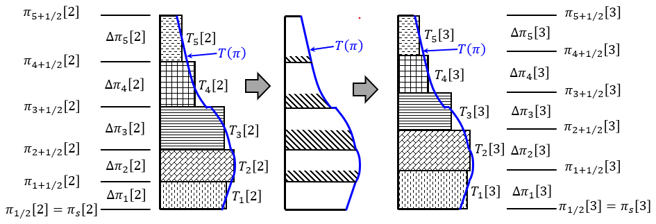
Figure B1 Schematic diagram of the vertical flux calculation in the vertically conservative semi-Lagrangian scheme. T(π) is an interpolation function obtained from the values of T_k[2]. The shaded areas in the middle subfigure represent the amounts moved from the upper to lower levels.

The integrated value S(π) from the top in the following equation is used instead of T(π):

$$\begin{array}{}\text{(B33)}& S\left(\mathit{\pi }\right)=\underset{{\mathit{\pi }}_{\mathrm{top}}}{\overset{\mathit{\pi }}{\int }}T\left({\mathit{\pi }}^{\prime }\right)\mathrm{d}{\mathit{\pi }}^{\prime }.\end{array}$$

The value $S\left({\mathit{\pi }}_{k-\mathrm{1}/\mathrm{2}\left[\mathrm{2}\right]}\right)$ is obtained from:

$$\begin{array}{}\text{(B34)}& \begin{array}{rl}S\left({\mathit{\pi }}_{k-\mathrm{1}/\mathrm{2}\left[\mathrm{2}\right]}\right)& =\underset{{\mathit{\pi }}_{\mathrm{top}}}{\overset{{\mathit{\pi }}_{k-\mathrm{1}/\mathrm{2}}\left[\mathrm{2}\right]}{\int }}T\left({\mathit{\pi }}^{\prime }\right)\mathrm{d}{\mathit{\pi }}^{\prime }\\ & =\sum _{l=k}^K{T}_l\left[\mathrm{2}\right]\mathrm{\Delta }{\mathit{\pi }}_l\left[\mathrm{2}\right].\end{array}\end{array}$$

There is arbitrariness in how to obtain the vertical profile of S(π). The third-order Lagrange interpolation is used to calculate the value S(π) from the values of $S\left({\mathit{\pi }}_{k-\mathrm{1}/\mathrm{2}}\left[\mathrm{2}\right]\right)$ at the nearest four grid points when ${\mathit{\pi }}_{\mathrm{3}/\mathrm{2}}\left[\mathrm{2}\right]\le \mathit{\pi }\le {\mathit{\pi }}_{K-\mathrm{1}/\mathrm{2}}\left[\mathrm{2}\right]$. Previously, when π is in the lowest or highest vertical levels, which is when ${\mathit{\pi }}_{\mathrm{1}/\mathrm{2}}\left[\mathrm{2}\right]\le \mathit{\pi }\le {\mathit{\pi }}_{\mathrm{3}/\mathrm{2}}\left[\mathrm{2}\right]$ or ${\mathit{\pi }}_{K-\mathrm{1}/\mathrm{2}}\left[\mathrm{2}\right]\le \mathit{\pi }\le {\mathit{\pi }}_{K+\mathrm{1}/\mathrm{2}}\left[\mathrm{2}\right]={\mathit{\pi }}_{\mathrm{top}}$, the third-order Lagrange interpolation was employed (i.e., the previous method) to calculate S(π) by using the extrapolated values of $S\left({\mathit{\pi }}_{-\mathrm{1}/\mathrm{2}}\left[\mathrm{2}\right]\right)$ and $S\left({\mathit{\pi }}_{K+\mathrm{3}/\mathrm{2}}\left[\mathrm{2}\right]\right)$:

$$\begin{array}{}\text{(B35a)}& {\displaystyle }S\left({\mathit{\pi }}_{-\mathrm{1}/\mathrm{2}}\left[\mathrm{2}\right]\right)=S\left({\mathit{\pi }}_{\mathrm{1}/\mathrm{2}}\left[\mathrm{2}\right]\right)+T_l\left[\mathrm{2}\right]\mathrm{\Delta }{\mathit{\pi }}_l\left[\mathrm{2}\right],\text{(B35b)}& {\displaystyle }S\left({\mathit{\pi }}_{K+\mathrm{3}/\mathrm{2}}\left[\mathrm{2}\right]\right)=S\left({\mathit{\pi }}_{K+\mathrm{1}/\mathrm{2}}\left[\mathrm{2}\right]\right)-T_K\left[\mathrm{2}\right]\mathrm{\Delta }{\mathit{\pi }}_K\left[\mathrm{2}\right].\end{array}$$

Here, the second-order Lagrange interpolation is used (i.e., the present method) instead of the third-order Lagrange interpolation when π is in the lowest or highest vertical levels. The values of $S\left({\mathit{\pi }}_{\mathrm{1}/\mathrm{2}}\left[\mathrm{2}\right]\right)$, $S\left({\mathit{\pi }}_{\mathrm{3}/\mathrm{2}}\left[\mathrm{2}\right]\right)$, and $S\left({\mathit{\pi }}_{\mathrm{5}/\mathrm{2}}\left[\mathrm{2}\right]\right)$ are used for interpolation when ${\mathit{\pi }}_{\mathrm{1}/\mathrm{2}}\left[\mathrm{2}\right]<\mathit{\pi }<{\mathit{\pi }}_{\mathrm{3}/\mathrm{2}}\left[\mathrm{2}\right]$, and the values of $S\left({\mathit{\pi }}_{K-\mathrm{3}/\mathrm{2}}\left[\mathrm{2}\right]\right)$, $S\left({\mathit{\pi }}_{K-\mathrm{1}/\mathrm{2}}\left[\mathrm{2}\right]\right),$ and $S\left({\mathit{\pi }}_{K+\mathrm{1}/\mathrm{2}}\left[\mathrm{2}\right]\right)$ are used when ${\mathit{\pi }}_{K-\mathrm{1}/\mathrm{2}}\left[\mathrm{2}\right]<\mathit{\pi }<{\mathit{\pi }}_{K+\mathrm{1}/\mathrm{2}}\left[\mathrm{2}\right]$. In the gravity wave test case (Sect. 3.7), the results of the present method are better than those of the previous method. Using the values of $S\left({\mathit{\pi }}_{k-\mathrm{1}/\mathrm{2}}\left[\mathrm{3}\right]\right)$ calculated by the Lagrange interpolation, T_k[3] is calculated as follows:

$$\begin{array}{}\text{(B36)}& T_k\left[\mathrm{3}\right]={\displaystyle \frac{\mathrm{1}}{\mathrm{\Delta }{\mathit{\pi }}_k\left[\mathrm{3}\right]}}\left[S\left({\mathit{\pi }}_{k-\mathrm{1}/\mathrm{2}}\left[\mathrm{3}\right]\right)-S\left({\mathit{\pi }}_{k+\mathrm{1}/\mathrm{2}}\left[\mathrm{3}\right]\right)\right].\end{array}$$

The value of T_k[5] can be calculated from T_k[4] in the same way using the values of Δπ_k[4] and Δπ_k[5].

In calculating the vertical flux of substances such as water vapor, the piecewise rational method (PRM; Xiao and Peng, 2004), which is a monotonic scheme, can be used to avoid negative values.

B4 Horizontal advection

Horizontal advection from [3] to [4] with Eqs. (B17) and (B19) is calculated using a typical two-dimensional horizontal semi-Lagrangian scheme. The horizontal departure point ${\left({\mathit{x}}_k\right)}_{D_{\mathrm{2}}\left(k\right)}$ is located upstream from the arrival point x_k along the wind vector between ${\left({\mathit{x}}_k\right)}_{D_{\mathrm{2}}\left(k\right)}$ and x_k.

One way to calculate ${\left({\mathit{x}}_k\right)}_{D_{\mathrm{2}}\left(k\right)}$ is to use the following equation:

$$\begin{array}{}\text{(B37)}& {\left({\mathit{x}}_k\right)}_{D_{\mathrm{2}}\left(k\right)}={\mathit{x}}_k-\mathrm{\Delta }t\left[{\displaystyle \frac{{\left({\mathit{v}}_k^{\left(+\right)}\left[\mathrm{3}\right]\right)}_{D_{\mathrm{2}}}+{\mathit{v}}_k^{\mathrm{0}}\left[{\mathrm{4}}^{\prime }\right]}{\mathrm{2}}}\right],\end{array}$$

where SETTLS is adopted, which uses the time-extrapolated future value ${\mathit{v}}_k^{\left(+\right)}=\mathrm{2}{\mathit{v}}_k^{\mathrm{0}}-{\mathit{v}}_k^{-}$ at the departure point ${\left({\mathit{x}}_k\right)}_{D_{\mathrm{2}}\left(k\right)}$. The variable ${\mathit{v}}_k^{\left(+\right)}\left[\mathrm{3}\right]$ is calculated by vertical remapping of ${\mathit{v}}_k^{\left(+\right)}\left[\mathrm{2}\right]$ using Δπ_k[2] and Δπ_k[3] (Appendix B3). The variable ${\mathit{v}}_k^{\mathrm{0}}\left[{\mathrm{4}}^{\prime }\right]$ is calculated by vertical remapping of ${\mathit{v}}_k^{\mathrm{0}}\left[{\mathrm{5}}^{\prime }\right]\left(={\mathit{v}}_k^{\mathrm{0}}\right)$, where Δπ_k[4^′] and Δπ_k[5^′] calculated from the following equations are used:

$$\begin{array}{}\text{(B38a)}& {\displaystyle }\mathrm{\Delta }{\mathit{\pi }}_k\left[{\mathrm{6}}^{\prime }\right]=\mathrm{\Delta }{A}_k+\mathrm{\Delta }{B}_k{\mathit{\pi }}_{\mathrm{s}}^{\mathrm{0}},\text{(B38b)}& {\displaystyle }\mathrm{\Delta }{\mathit{\pi }}_k\left[{\mathrm{5}}^{\prime }\right]=\mathrm{\Delta }{\mathit{\pi }}_k\left[{\mathrm{6}}^{\prime }\right]+{\displaystyle \frac{\mathrm{\Delta }t}{\mathrm{2}}}{\left(D_k\mathrm{\Delta }{\mathit{\pi }}_k\right)}^{\mathrm{0}},\text{(B38c)}& {\displaystyle }\begin{array}{rl}\mathrm{\Delta }{\mathit{\pi }}_k\left[{\mathrm{4}}^{\prime }\right]& =\mathrm{\Delta }{\mathit{\pi }}_k\left[{\mathrm{5}}^{\prime }\right]+{\displaystyle \frac{\mathrm{\Delta }t}{\mathrm{2}}}\left[\right(\dot{\mathit{\eta }}{\displaystyle \frac{\partial \mathit{\pi }}{\partial \mathit{\eta }}}{)}_{k-\mathrm{1}/\mathrm{2}}^{\mathrm{0}}\\ & -\left(\dot{\mathit{\eta }}{\displaystyle \frac{\partial \mathit{\pi }}{\partial \mathit{\eta }}}{)}_{k+\mathrm{1}/\mathrm{2}}^{\mathrm{0}}\right].\end{array}\end{array}$$

Here, Eq. (B38a) is derived from Eqs. (B28) and (B25), where ${\mathit{\pi }}_{\mathrm{s}}^{+,\mathrm{explicit}}$ is approximated by ${\mathit{\pi }}_{\mathrm{s}}^{\mathrm{0}}$. Equations (B38b) and (B38c) are derived from Eqs. (B22) and (B20), respectively. It is better to use ${\mathit{v}}_k^{\mathrm{0}}\left[\mathrm{4}\right]$ instead of ${\mathit{v}}_k^{\mathrm{0}}\left[{\mathrm{4}}^{\prime }\right]$ in Eq. (B37). However, when calculating horizontal advection from [3] to [4], Δπ_k[4] and Δπ_k[5] are not yet obtained, and ${\mathit{v}}_k^{\mathrm{0}}\left[\mathrm{4}\right]$ cannot be calculated. Therefore, in Eq. (B37), ${\mathit{v}}_k^{\mathrm{0}}\left[{\mathrm{4}}^{\prime }\right]$ is used as a sufficiently accurate approximation of ${\mathit{v}}_k^{\mathrm{0}}\left[\mathrm{4}\right]$.

By using Eq. (B37), the horizontal departure point ${\left({\mathit{x}}_k\right)}_{D_{\mathrm{2}}}$ can be calculated by iteration (e.g., Ritchie et al., 1995; Temperton et al., 2001). The value of ${\left({\mathit{v}}_k^{\left(+\right)}\left[\mathrm{3}\right]\right)}_{D_{\mathrm{2}}}$ at the horizontal departure point ${\left({\mathbf{x}}_k\right)}_{D_{\mathrm{2}}}$ is calculated by the Lagrange interpolation from the values at the grid points near ${\left({\mathbf{x}}_k\right)}_{D_{\mathrm{2}}}$. Here, the fifth-order Lagrange interpolation is used.

The explicitly calculated provisional future value of the wind (Yoshimura, 2022) can also be used instead of the extrapolated future value ${\mathit{v}}_k^{\left(+\right)}$. ${\mathit{v}}_k^{\left(+\right)}$ is used here because the results of the test cases in Sect. 3 are almost identical when the explicitly calculated provisional future value is used.

B5 Horizontal advection of a variable at half-levels

When calculating the advection $w_{k+\mathrm{1}/\mathrm{2}}$ at half levels to obtain ${\left(w_{k+\mathrm{1}/\mathrm{2}}\right)}_{\mathrm{D}}$, $w_{k+\mathrm{1}/\mathrm{2}}$ is converted to w_k at full levels using the following equation:

$$\begin{array}{}\text{(B39)}& w_k={\displaystyle \frac{w_{k-\mathrm{1}/\mathrm{2}}+w_{k+\mathrm{1}/\mathrm{2}}}{\mathrm{2}}},\end{array}$$

and then the advection of w_k is calculated using the vertically conservative semi-Lagrangian scheme provided in Appendix B2 to obtain ${\left(w_k\right)}_{\mathrm{D}}$. The value of ${\left(w_{k+\mathrm{1}/\mathrm{2}}\right)}_{\mathrm{D}}$ is calculated from the following equation:

$$\begin{array}{}\text{(B40)}& \begin{array}{rl}{\left(w_{k+\mathrm{1}/\mathrm{2}}\right)}_{\mathrm{D}}& =w_{k+\mathrm{1}/\mathrm{2}}\\ & +{\displaystyle \frac{\left(\begin{array}{c}\ln \left(\frac{{\mathit{\pi }}_{k-\mathrm{1}/\mathrm{2}}}{{\mathit{\pi }}_{k+\mathrm{1}/\mathrm{2}}}\right)\left[{\left(w_k\right)}_{\mathrm{D}}-w_k\right]\\ +\ln \left(\frac{{\mathit{\pi }}_{k+\mathrm{1}/\mathrm{2}}}{{\mathit{\pi }}_{k+\mathrm{3}/\mathrm{2}}}\right)\left[{\left(w_{k+\mathrm{1}}\right)}_{\mathrm{D}}-w_{k+\mathrm{1}}\right]\end{array}\right)}{\ln \left(\frac{{\mathit{\pi }}_{k-\mathrm{1}/\mathrm{2}}}{{\mathit{\pi }}_{k+\mathrm{1}/\mathrm{2}}}\right)+\ln \left(\frac{{\mathit{\pi }}_{k+\mathrm{1}/\mathrm{2}}}{{\mathit{\pi }}_{k+\mathrm{3}/\mathrm{2}}}\right)}}.\end{array}\end{array}$$

The method of vertically interpolating ${\left(w_k\right)}_{\mathrm{D}}-w_k$ using Eq. (B40) to obtain ${\left(w_{k+\mathrm{1}/\mathrm{2}}\right)}_{\mathrm{D}}$ is more accurate than simply vertically interpolating ${\left(w_k\right)}_{\mathrm{D}}$.

B6 Spatially averaged Eulerian treatment of mountains with horizontal mass advection

The spatially averaged Eulerian treatment of mountains, similar to that of Ritchie and Tanguay (1996) for a shallow-water model, is adopted when the horizontal mass advection is calculated. Ritchie and Tanguay (1996) showed that this type of treatment alleviates numerical problems associated with orographic forcing in semi-implicit semi-Lagrangian models. The approximate effect of Φ_s on the surface pressure is defined here as

$$\begin{array}{}\text{(B41)}& {\mathit{\pi }}_{\mathrm{s}}^{\mathrm{\Phi }}\equiv {\stackrel{\mathrm{̃}}{\mathit{\pi }}}_{\mathrm{s}}\exp \left({\displaystyle \frac{-{\mathrm{\Phi }}_{\mathrm{s}}}{R\stackrel{\mathrm{̃}}{T}}}\right),\end{array}$$

where ${\stackrel{\mathrm{̃}}{\mathit{\pi }}}_{\mathrm{s}}={\mathrm{10}}^{\mathrm{5}}$ (Pa) and $\stackrel{\mathrm{̃}}{T}=\mathrm{280}$ (K). Since $\partial {\mathit{\pi }}_{\mathrm{s}}^{\mathrm{\Phi }}/\partial t=\mathrm{0}$, the following equation is satisfied:

$$\begin{array}{}\text{(B42)}& {\displaystyle \frac{{\mathrm{d}}_H}{\mathrm{d}t}}\left(\mathrm{\Delta }{\mathit{\pi }}_k^{\mathrm{\Phi }}\right)={\displaystyle \frac{{\mathrm{d}}_H}{\mathrm{d}t}}\left(\mathrm{\Delta }{B}_k{\mathit{\pi }}_{\mathrm{s}}^{\mathrm{\Phi }}\right)=\mathrm{\Delta }{B}_k{\mathit{v}}_k\cdot \mathrm{\nabla }{\mathit{\pi }}_{\mathrm{s}}^{\mathrm{\Phi }},\end{array}$$

where $\mathrm{\Delta }{\mathit{\pi }}_k^{\mathrm{\Phi }}\equiv \mathrm{\Delta }{A}_k+\mathrm{\Delta }{B}_k{\mathit{\pi }}_{\mathrm{s}}^{\mathrm{\Phi }}$. Using Eq. (B42), Eq. (B5) becomes

$$\begin{array}{}\text{(B43)}& \begin{array}{rl}{\displaystyle \frac{{\mathrm{d}}_H}{\mathrm{d}t}}\left(\mathrm{\Delta }{\mathit{\pi }}_k-\mathrm{\Delta }{B}_k{\mathit{\pi }}_{\mathrm{s}}^{\mathrm{\Phi }}\right)& =-\mathrm{\Delta }{B}_k{\mathit{v}}_k\cdot \mathrm{\nabla }{\mathit{\pi }}_{\mathrm{s}}^{\mathrm{\Phi }}-D_k\mathrm{\Delta }{\mathit{\pi }}_k\\ & -{\left(\dot{\mathit{\eta }}{\displaystyle \frac{\partial \mathit{\pi }}{\partial \mathit{\eta }}}\right)}_{k-\mathrm{1}/\mathrm{2}}+{\left(\dot{\mathit{\eta }}{\displaystyle \frac{\partial \mathit{\pi }}{\partial \mathit{\eta }}}\right)}_{k+\mathrm{1}/\mathrm{2}}.\end{array}\end{array}$$

By discretizing Eq. (B43) in time in the same way as Eq. (B7), and using Eqs. (B9), (B11), (B14), (B20), (B22), and (B25), the following equation is obtained:

$$\begin{array}{}\text{(B44)}& \begin{array}{rl}\mathrm{\Delta }{\mathit{\pi }}_k\left[\mathrm{4}\right]& =[\mathrm{\Delta }{\mathit{\pi }}_k\left[\mathrm{3}\right]-\mathrm{\Delta }{B}_k{\mathit{\pi }}_{\mathrm{s}}^{\mathrm{\Phi }}\\ & -{\displaystyle \frac{\mathrm{\Delta }t}{\mathrm{2}}}\mathrm{\Delta }{B}_k{\mathit{v}}_k^{\left(+\right)}\left[\mathrm{3}\right]\cdot \mathrm{\nabla }{\mathit{\pi }}_{\mathrm{s}}^{\mathrm{\Phi }}{]}_{D_{\mathrm{2}}\left(k\right)}\\ & +\mathrm{\Delta }{B}_k{\mathit{\pi }}_{\mathrm{s}}^{\mathrm{\Phi }}-{\displaystyle \frac{\mathrm{\Delta }t}{\mathrm{2}}}\mathrm{\Delta }{B}_k{\mathit{v}}_k\left[{\mathrm{4}}^{\prime }\right]\cdot \mathrm{\nabla }{\mathit{\pi }}_{\mathrm{s}}^{\mathrm{\Phi }}.\end{array}\end{array}$$

By using Eq. (B44) instead of Eq. (B17), the results near mountains are improved (Sect. 3.4).

B7 Semi-Lagrangian treatment of hydrostatic pressure change due to horizontal advection

Equation (C17c) below includes:

$$\begin{array}{}\text{(B45)}& \begin{array}{rl}{\left(\mathit{\delta }\mathit{\pi }\right)}_k& \equiv B_{k+\mathrm{1}/\mathrm{2}}{\mathit{\pi }}_{\mathrm{s}}{\mathit{v}}_k\cdot \mathrm{\nabla }\ln {\mathit{\pi }}_{\mathrm{s}}\\ & -\sum _{l=k+\mathrm{1}}^K\left(\mathrm{\Delta }{B}_l{\mathit{\pi }}_{\mathrm{s}}{\mathit{v}}_l\cdot \mathrm{\nabla }\ln {\mathit{\pi }}_{\mathrm{s}}\right)\\ & ={\mathit{v}}_k\cdot \mathrm{\nabla }{\mathit{\pi }}_{k+\mathrm{1}/\mathrm{2}}-\sum _{l=k+\mathrm{1}}^K\left({\mathit{v}}_l\cdot \mathrm{\nabla }\left(\mathrm{\Delta }{\mathit{\pi }}_l\right)\right),\end{array}\end{array}$$

which represents the hydrostatic pressure change due to horizontal advection. The term ${\mathit{v}}_k\cdot \mathrm{\nabla }{\mathit{\pi }}_{k+\mathrm{1}/\mathrm{2}}$ represents the pressure change due to horizontal advection in the kth layer, and the term $-\sum _{l=k+\mathrm{1}}^K\left({\mathit{v}}_l\cdot \mathrm{\nabla }\left(\mathrm{\Delta }{\mathit{\pi }}_l\right)\right)$ represents the pressure change due to horizontal advection of mass in the layers above the kth layer. The nonlinear terms related to horizontal advection in Eq. (B45) can be one of the sources of numerical instability with long timesteps. δπ can be evaluated more appropriately in a semi-Lagrangian manner as follows:

$$\begin{array}{}\text{(B46)}& {\left(\mathit{\delta }\mathit{\pi }\right)}_k={\displaystyle \frac{{\mathit{\pi }}_{k+\mathrm{1}/\mathrm{2}}\left[\mathrm{4}\right]-{\mathit{\pi }}_{k+\mathrm{1}/\mathrm{2}}{\left[\mathrm{3}\right]}_{D_{\mathrm{2}}\left(k\right)}}{\mathrm{\Delta }t}}.\end{array}$$

Using Eqs. (B46) and (B17), Eq. (C17c) can be discretized as follows:

$$\begin{array}{}\text{(B47)}& \begin{array}{rl}& {\left(F_{Q\left(\mathrm{adv}\right)}\right)}_k\mathrm{\Delta }t=-{\displaystyle \frac{\mathrm{1}}{\mathrm{2}}}[{\displaystyle \frac{\mathrm{1}}{\mathrm{\Delta }{\mathit{\pi }}_k\left[\mathrm{4}\right]}}\ln \left({\displaystyle \frac{{\mathit{\pi }}_{k-\mathrm{1}/\mathrm{2}}\left[\mathrm{4}\right]}{{\mathit{\pi }}_{k+\mathrm{1}/\mathrm{2}}\left[\mathrm{4}\right]}}\right)\\ & +{\left\{{\displaystyle \frac{\mathrm{1}}{\mathrm{\Delta }{\mathit{\pi }}_k\left[\mathrm{3}\right]}}\ln \left({\displaystyle \frac{{\mathit{\pi }}_{k-\mathrm{1}/\mathrm{2}}\left[\mathrm{3}\right]}{{\mathit{\pi }}_{k+\mathrm{1}/\mathrm{2}}\left[\mathrm{3}\right]}}\right)\right\}}_{D_{\mathrm{2}}\left(k\right)}]{\left(\mathit{\delta }\mathit{\pi }\right)}_k\mathrm{\Delta }t\\ & =-{\displaystyle \frac{\mathrm{1}}{\mathrm{2}\mathrm{\Delta }{\mathit{\pi }}_k\left[\mathrm{4}\right]}}\ln ({\displaystyle \frac{{\mathit{\pi }}_{k-\mathrm{1}/\mathrm{2}}\left[\mathrm{4}\right]}{{\mathit{\pi }}_{k+\mathrm{1}/\mathrm{2}}\left[\mathrm{4}\right]}}\\ & \cdot {\displaystyle \frac{{\mathit{\pi }}_{k+\mathrm{1}/\mathrm{2}}{\left[\mathrm{3}\right]}_{D_{\mathrm{2}}\left(k\right)}+\mathrm{\Delta }{\mathit{\pi }}_k\left[\mathrm{4}\right]}{{\mathit{\pi }}_{k+\mathrm{1}/\mathrm{2}}{\left[\mathrm{3}\right]}_{D_{\mathrm{2}}\left(k\right)}}})\\ & \cdot \left({\mathit{\pi }}_{k+\mathrm{1}/\mathrm{2}}\left[\mathrm{4}\right]-{\mathit{\pi }}_{k+\mathrm{1}/\mathrm{2}}{\left[\mathrm{3}\right]}_{D_{\mathrm{2}}\left(k\right)}\right).\end{array}\end{array}$$

Using Eq. (B47), instead of discretizing Eq. (C17c) in the usual way, improves the results in some cases when the timestep is long (Sect. 3.4). A similar semi-Lagrangian treatment is also used in the hydrostatic option of the model.

B8 Cubic Hermite interpolation to calculate the change in hydrostatic pressure with horizontal advection

To calculate ${\mathit{\pi }}_{k+\mathrm{1}/\mathrm{2}}{\left[\mathrm{3}\right]}_{D_{\mathrm{2}}\left(k\right)}$ at the horizontal departure point in Eq. (B47), piecewise cubic Hermite interpolation is used. The cubic Hermite interpolation requires the horizontal derivative and is computationally expensive if the horizontal derivative of ${\mathit{\pi }}_{k+\mathrm{1}/\mathrm{2}}\left[\mathrm{3}\right]$ is calculated every timestep by transforming ${\mathit{\pi }}_{k+\mathrm{1}/\mathrm{2}}\left[\mathrm{3}\right]$ from grid to spectral space and the horizontal derivative of ${\mathit{\pi }}_{k+\mathrm{1}/\mathrm{2}}\left[\mathrm{3}\right]$ from spectral to grid space. Since ${\mathit{\pi }}_{k+\mathrm{1}/\mathrm{2}}\left[\mathrm{3}\right]$ has similar values to $f_{k+\mathrm{1}/\mathrm{2}}=A_{k+\mathrm{1}/\mathrm{2}}+B_{k+\mathrm{1}/\mathrm{2}}{\mathit{\pi }}_{\mathrm{s}}^{\mathrm{\Phi }}$ (Eq. B41) and the horizontal derivative $\partial f_{k+\mathrm{1}/\mathrm{2}}/\partial x=B_{k+\mathrm{1}/\mathrm{2}}\partial {\mathit{\pi }}_{\mathrm{s}}^{\mathrm{\Phi }}/\partial x$ only needs to be calculated once rather than at every timestep, $f_{k+\mathrm{1}/\mathrm{2}}$ is interpolated using the cubic Hermite interpolation and the remaining $g_{k+\mathrm{1}/\mathrm{2}}={\mathit{\pi }}_{k+\mathrm{1}/\mathrm{2}}\left[\mathrm{3}\right]-f_{k+\mathrm{1}/\mathrm{2}}$ is interpolated using the fifth-order Lagrange interpolation. This method yields slightly better results than using only the fifth-order Lagrange interpolation in case Schär2 when the timestep is short and the departure point is near a grid point (Sect. 3.4).

Appendix C: Vertical discretization

The following vertical discretization method is used, which is similar to that of Bubnová et al. (1995), except for Eqs. (C1)–(C3) and (C19)–(C21) where the discretization is similar to that of Simmons and Burridge (1981):

$$\begin{array}{}\text{(C1)}& {\displaystyle }{\mathit{\delta }}_k\equiv \left\{\begin{array}{ll}\ln \frac{{\mathit{\pi }}_{k-\mathrm{1}/\mathrm{2}}}{{\mathit{\pi }}_{k+\mathrm{1}/\mathrm{2}}}& \mathrm{for}k<K\\ \mathrm{2}\ln \mathrm{2}& \mathrm{for}k=K,\end{array}\right.\text{(C2)}& {\displaystyle }{\stackrel{\mathrm{̃}}{\mathit{\pi }}}_k={\displaystyle \frac{\mathrm{\Delta }{\mathit{\pi }}_k}{{\mathit{\delta }}_k}},\text{(C3)}& {\displaystyle }{\mathit{\alpha }}_k\equiv \left\{\begin{array}{ll}\mathrm{1}-\frac{{\mathit{\pi }}_{k+\mathrm{1}/\mathrm{2}}}{{\stackrel{\mathrm{̃}}{\mathit{\pi }}}_k}& \mathrm{for}k<K\\ \ln \mathrm{2}& \mathrm{for}k=K,\end{array}\right.\text{(C4)}& {\displaystyle }\mathrm{\nabla }{\mathit{\pi }}_{\mathrm{s}}={\mathit{\pi }}_{\mathrm{s}}\mathrm{\nabla }\ln {\mathit{\pi }}_{\mathrm{s}},\text{(C5)}& {\displaystyle }{\mathrm{\Phi }}_{k-\mathrm{1}/\mathrm{2}}={\mathrm{\Phi }}_{\mathrm{s}}+\sum _{l=\mathrm{1}}^{k-\mathrm{1}}\left({\mathit{\delta }}_l{\displaystyle \frac{R{T}_l}{\mathrm{1}+{\mathcal{P}}_l}}\right),\text{(C6)}& {\displaystyle }{\mathrm{\Phi }}_k={\mathrm{\Phi }}_{k-\mathrm{1}/\mathrm{2}}+{\mathit{\alpha }}_k{\displaystyle \frac{R{T}_k}{\mathrm{1}+{\mathcal{P}}_k}},\text{(C7)}& {\displaystyle }\begin{array}{rl}\mathrm{\nabla }{\mathrm{\Phi }}_{k-\mathrm{1}/\mathrm{2}}& =\mathrm{\nabla }{\mathrm{\Phi }}_{\mathrm{s}}+\sum _{l=\mathrm{1}}^{k-\mathrm{1}}[{\mathit{\delta }}_{l}R\left({\displaystyle \frac{\mathrm{\nabla }{T}_l-T_l\mathrm{\nabla }{\mathcal{Q}}_l}{\mathrm{1}+{\mathcal{P}}_l}}\right)\\ & +{\displaystyle \frac{R{T}_l}{\mathrm{1}+{\mathcal{P}}_l}}\left({\displaystyle \frac{B_{l-\mathrm{1}/\mathrm{2}}}{{\mathit{\pi }}_{l-\mathrm{1}/\mathrm{2}}}}-{\displaystyle \frac{B_{l+\mathrm{1}/\mathrm{2}}}{{\mathit{\pi }}_{l+\mathrm{1}/\mathrm{2}}}}\right)\mathrm{\nabla }{\mathit{\pi }}_{\mathrm{s}}],\end{array}\text{(C8)}& {\displaystyle }{\left(\mathrm{\nabla }\ln \mathit{\pi }\right)}_k={\displaystyle \frac{{\mathit{\delta }}_k{B}_{k+\mathrm{1}/\mathrm{2}}+{\mathit{\alpha }}_k\mathrm{\Delta }{B}_k}{\mathrm{\Delta }{\mathit{\pi }}_k}}\mathrm{\nabla }{\mathit{\pi }}_{\mathrm{s}},\text{(C9)}& {\displaystyle }\begin{array}{rl}\mathrm{\nabla }{\mathrm{\Phi }}_k& =\mathrm{\nabla }{\mathrm{\Phi }}_{k-\mathrm{1}/\mathrm{2}}+{\mathit{\alpha }}_{k}R\left({\displaystyle \frac{\mathrm{\nabla }{T}_k-T_k\mathrm{\nabla }{\mathcal{Q}}_k}{\mathrm{1}+{\mathcal{P}}_k}}\right)\\ & +{\displaystyle \frac{R{T}_k}{\mathrm{1}+{\mathcal{P}}_k}}{\displaystyle \frac{B_{k-\mathrm{1}/\mathrm{2}}}{{\mathit{\pi }}_{k-\mathrm{1}/\mathrm{2}}}}\mathrm{\nabla }{\mathit{\pi }}_{\mathrm{s}}-{\displaystyle \frac{R{T}_k}{\mathrm{1}+{\mathcal{P}}_k}}{\left(\mathrm{\nabla }\ln \mathit{\pi }\right)}_k,\end{array}\text{(C10)}& {\displaystyle }{\left({\displaystyle \frac{\mathrm{1}}{m}}{\displaystyle \frac{\partial \mathit{\pi }\mathcal{P}}{\partial \mathit{\eta }}}\right)}_{k-\mathrm{1}/\mathrm{2}}=\left\{\begin{array}{ll}\text{See Sect. 2.3 }& \mathrm{for}k=\mathrm{1}\\ \frac{{\stackrel{\mathrm{̃}}{\mathit{\pi }}}_k{\mathcal{P}}_k-{\stackrel{\mathrm{̃}}{\mathit{\pi }}}_{k+\mathrm{1}}{\mathcal{P}}_{k+\mathrm{1}}}{{\stackrel{\mathrm{̃}}{\mathit{\pi }}}_k-{\stackrel{\mathrm{̃}}{\mathit{\pi }}}_{k+\mathrm{1}}}& \mathrm{for}\mathrm{2}\le k\le K\\ {\mathcal{P}}_k& \mathrm{for}k=K+\mathrm{1},\end{array}\right.\text{(C11)}& {\displaystyle }\begin{array}{rl}{\left({\mathit{F}}_v\right)}_k& =-R{T}_k\left[{\left(\mathrm{\nabla }\ln \mathit{\pi }\right)}_k+\mathrm{\nabla }{\mathcal{Q}}_k\right]-\mathrm{\nabla }{\mathrm{\Phi }}_k\\ & -{\displaystyle \frac{\mathrm{1}}{\mathrm{2}}}\left[{\left({\displaystyle \frac{\mathrm{1}}{m}}{\displaystyle \frac{\partial \mathit{\pi }\mathcal{P}}{\partial \mathit{\eta }}}\right)}_{k-\mathrm{1}/\mathrm{2}}+{\left({\displaystyle \frac{\mathrm{1}}{m}}{\displaystyle \frac{\partial \mathit{\pi }\mathcal{P}}{\partial \mathit{\eta }}}\right)}_{k+\mathrm{1}/\mathrm{2}}\right]\mathrm{\nabla }{\mathrm{\Phi }}_k,\end{array}\text{(C12)}& {\displaystyle }{\left(F_w\right)}_{k-\mathrm{1}/\mathrm{2}}=g{\left({\displaystyle \frac{\mathrm{1}}{m}}{\displaystyle \frac{\partial \mathit{\pi }\mathcal{P}}{\partial \mathit{\eta }}}\right)}_{k-\mathrm{1}/\mathrm{2}},\text{(C13)}& {\displaystyle }{\mathit{v}}_{k-\mathrm{1}/\mathrm{2}}={\displaystyle \frac{{\mathit{\delta }}_k{\mathit{v}}_{k-\mathrm{1}}+{\mathit{\delta }}_{k-\mathrm{1}}{\mathit{v}}_k}{{\mathit{\delta }}_{k-\mathrm{1}}+{\mathit{\delta }}_k}},\text{(C14)}& {\displaystyle }\begin{array}{rl}{\left(D_{\mathrm{3}}\right)}_k& =\mathit{\{}\mathrm{\nabla }\cdot \mathit{v}+{\displaystyle \frac{\left(\mathrm{1}+\mathcal{P}\right)}{RT}}{\displaystyle \frac{\mathit{\pi }}{m}}[{\displaystyle \frac{\partial }{\partial \mathit{\eta }}}\left(\mathrm{\nabla }\mathrm{\Phi }\cdot \mathit{v}\right)\\ & -{\displaystyle \frac{\partial \mathrm{\nabla }\mathrm{\Phi }}{\partial \mathit{\eta }}}\cdot \mathit{v}]-{\displaystyle \frac{\left(\mathrm{1}+\mathcal{P}\right)\mathit{\pi }}{RT}}{\displaystyle \frac{g}{m}}{\displaystyle \frac{\partial w}{\partial \mathit{\eta }}}{\mathit{\}}}_k\\ & =D_k+{\displaystyle \frac{\mathrm{1}+{\mathcal{P}}_k}{R{T}_k}}{\displaystyle \frac{{\stackrel{\mathrm{̃}}{\mathit{\pi }}}_k}{\mathrm{\Delta }{\mathit{\pi }}_k}}[\mathrm{\nabla }{\mathrm{\Phi }}_{k-\mathrm{1}/\mathrm{2}}\cdot {\mathit{v}}_{k-\mathrm{1}/\mathrm{2}}\\ & -\mathrm{\nabla }{\mathrm{\Phi }}_{k+\mathrm{1}/\mathrm{2}}\cdot {\mathit{v}}_{k+\mathrm{1}/\mathrm{2}}-\left(\mathrm{\nabla }{\mathrm{\Phi }}_{k-\mathrm{1}/\mathrm{2}}-\mathrm{\nabla }{\mathrm{\Phi }}_{k+\mathrm{1}/\mathrm{2}}\right)\cdot {\mathit{v}}_k\\ & -g\left(w_{k-\mathrm{1}/\mathrm{2}}-w_{k+\mathrm{1}/\mathrm{2}}\right)],\end{array}\text{(C14')}& {\displaystyle }\begin{array}{rl}{\left(D_{\mathrm{3}}\right)}_{k=\mathrm{1}}& =D_k+{\displaystyle \frac{\mathrm{1}+{\mathcal{P}}_l}{R{T}_l}}{\displaystyle \frac{{\stackrel{\mathrm{̃}}{\mathit{\pi }}}_{\mathrm{1}}}{\mathrm{\Delta }{\mathit{\pi }}_l}}[-\mathrm{\nabla }{\mathrm{\Phi }}_{\mathrm{3}/\mathrm{2}}\cdot {\mathit{v}}_{\mathrm{3}/\mathrm{2}}\\ & -\left(\mathrm{\nabla }{\mathrm{\Phi }}_{\mathrm{1}/\mathrm{2}}-\mathrm{\nabla }{\mathrm{\Phi }}_{\mathrm{3}/\mathrm{2}}\right)\cdot {\mathit{v}}_l-g\left(-w_{\mathrm{3}/\mathrm{2}}\right)],\end{array}\text{(C15)}& {\displaystyle }{\left(F_{\ln T}\right)}_k=-{\displaystyle \frac{R}{c_v}}{\left(D_{\mathrm{3}}\right)}_k,\text{(C16)}& {\displaystyle }\begin{array}{rl}{\left({\displaystyle \frac{\mathrm{1}}{\mathit{\pi }}}{\displaystyle \frac{\mathrm{d}\mathit{\pi }}{\mathrm{d}t}}\right)}_k& ={\displaystyle \frac{\mathrm{1}}{\mathrm{\Delta }{\mathit{\pi }}_k}}\mathit{\left\{}\ln \left({\displaystyle \frac{{\mathit{\pi }}_{k-\mathrm{1}/\mathrm{2}}}{{\mathit{\pi }}_{k+\mathrm{1}/\mathrm{2}}}}\right)\right[B_{k+\mathrm{1}/\mathrm{2}}{\mathit{\pi }}_{\mathrm{s}}{\mathit{v}}_k\cdot \mathrm{\nabla }\ln {\mathit{\pi }}_{\mathrm{s}}\\ & -\sum _{l=k+\mathrm{1}}^K\left(\mathrm{\Delta }{B}_l{\mathit{\pi }}_{\mathrm{s}}{\mathit{v}}_l\cdot \mathrm{\nabla }\ln {\mathit{\pi }}_{\mathrm{s}}+D_{\mathrm{1}}\mathrm{\Delta }{\mathit{\pi }}_l\right)]\\ & -{\mathit{\alpha }}_k{D}_k\mathrm{\Delta }{\mathit{\pi }}_k\mathit{\}},\end{array}\end{array}$$

$$\begin{array}{}\text{(C17a)}& {\displaystyle }\begin{array}{rl}{F}_{\mathcal{Q}}& =-{\left({\displaystyle \frac{\mathrm{1}}{\mathit{\pi }}}{\displaystyle \frac{\mathrm{d}\mathit{\pi }}{\mathrm{d}t}}\right)}_k-{\displaystyle \frac{c_{\mathrm{p}}}{c_{\mathrm{v}}}}{\left(D_{\mathrm{3}}\right)}_k\\ & ={\left(F_{Q\left(\mathrm{div}\right)}\right)}_k+{\left(F_{Q\left(\mathrm{adv}\right)}\right)}_k,\end{array}\text{(C17b)}& {\displaystyle }\begin{array}{rl}{\left(F_{Q\left(\mathrm{div}\right)}\right)}_k& \equiv -{\displaystyle \frac{c_{\mathrm{p}}}{c_v}}{\left(D_{\mathrm{3}}\right)}_k\\ & +\left[{\displaystyle \frac{\mathrm{1}}{\mathrm{\Delta }{\mathit{\pi }}_k}}\ln \right({\displaystyle \frac{{\mathit{\pi }}_{k-\mathrm{1}/\mathrm{2}}}{{\mathit{\pi }}_{k+\mathrm{1}/\mathrm{2}}}})\sum _{l=k+\mathrm{1}}^K\left(D_{\mathrm{1}}\mathrm{\Delta }{\mathit{\pi }}_l\right)\\ & +{\mathit{\alpha }}_k{D}_k\mathrm{\Delta }{\mathit{\pi }}_k],\end{array}\text{(C17c)}& {\displaystyle }\begin{array}{rl}{\left(F_{Q\left(\mathrm{adv}\right)}\right)}_k& \equiv {\displaystyle \frac{\mathrm{1}}{\mathrm{\Delta }{\mathit{\pi }}_k}}\ln \left({\displaystyle \frac{{\mathit{\pi }}_{k-\mathrm{1}/\mathrm{2}}}{{\mathit{\pi }}_{k+\mathrm{1}/\mathrm{2}}}}\right)[-B_{k+\mathrm{1}/\mathrm{2}}{\mathit{\pi }}_{\mathrm{s}}{\mathit{v}}_k\cdot \mathrm{\nabla }\ln {\mathit{\pi }}_{\mathrm{s}}\\ & +\sum _{l=k+\mathrm{1}}^K\left(\mathrm{\Delta }{B}_l{\mathit{\pi }}_{\mathrm{s}}{\mathit{v}}_l\cdot \mathrm{\nabla }\ln {\mathit{\pi }}_{\mathrm{s}}\right)],\end{array}\end{array}$$

$$\begin{array}{}\text{(C18)}& {\displaystyle }\mathrm{\Delta }{\mathit{\pi }}_k^{*}=\mathrm{\Delta }{A}_k+\mathrm{\Delta }{B}_k{\stackrel{\mathrm{‾}}{\mathit{\pi }}}_{\mathrm{s}},\text{(C19)}& {\displaystyle }{\mathit{\delta }}_k^{*}=\left\{\begin{array}{ll}\ln \left({\mathit{\pi }}_{k-\mathrm{1}/\mathrm{2}}^{*}/{\mathit{\pi }}_{k+\mathrm{1}/\mathrm{2}}^{*}\right)& \mathrm{for}\mathrm{1}\le k\le K-\mathrm{1}\\ \mathrm{2}\ln \mathrm{2}& \mathrm{for}k=K,\end{array}\right.\text{(C20)}& {\displaystyle }{\stackrel{\mathrm{̃}}{\mathit{\pi }}}_k^{*}=\mathrm{\Delta }{\mathit{\pi }}_{\mathrm{1}}^{*}/{\mathit{\delta }}_l^{*},\text{(C21)}& {\displaystyle }{\mathit{\alpha }}_k^{*}=\left\{\begin{array}{ll}\mathrm{1}-\frac{{\mathit{\pi }}_{k+\mathrm{1}/\mathrm{2}}^{*}}{{\stackrel{\mathrm{̃}}{\mathit{\pi }}}_k^{*}}& \mathrm{for}\mathrm{1}\le k\le K-\mathrm{1}\\ \ln \mathrm{2}& \mathrm{for}k=K,\end{array}\right.\text{(C22)}& {\displaystyle }{\left({\displaystyle \frac{{\mathit{\pi }}^{*}}{m^{*}}}{\displaystyle \frac{\partial X}{\partial \mathit{\eta }}}\right)}_k={\displaystyle \frac{X_{k-\mathrm{1}/\mathrm{2}}-X_{k+\mathrm{1}/\mathrm{2}}}{{\mathit{\delta }}_k^{*}}},\end{array}$$

$$\begin{array}{}\text{(C23a)}& {\displaystyle }\begin{array}{rl}{\left({\mathit{L}}_{\mathrm{C},v}\right)}_k& =R\stackrel{\mathrm{‾}}{T}[{\left\{{\mathbf{G}}^{*}\left(-\mathrm{\nabla }\ln T+\mathrm{\nabla }\mathcal{Q}\right)\right\}}_k\\ & -\mathrm{\nabla }{\mathcal{Q}}_k-\mathrm{\nabla }\ln {\mathit{\pi }}_{\mathrm{s}}],\end{array}\text{(C23b)}& {\displaystyle }{\left({\mathbf{G}}^{*}X\right)}_k\equiv \sum _{l=\mathrm{1}}^{k-\mathrm{1}}{\mathit{\delta }}_l^{*}{X}_l+{\mathit{\alpha }}_k^{*}{X}_k,\end{array}$$

$$\begin{array}{}\text{(C24)}& {\displaystyle }\begin{array}{rl}{\left({\mathit{L}}_{\mathrm{N},v}\right)}_k& =-{\left[\mathrm{\nabla }{\mathrm{\Phi }}^{\mathit{\#}}{\displaystyle \frac{\mathrm{1}}{m^{\mathit{\#}}}}{\displaystyle \frac{\partial \left({\mathit{\pi }}^{\mathit{\#}}\mathcal{P}\right)}{\partial \mathit{\eta }}}\right]}_k\\ & =-\mathrm{\nabla }{\mathrm{\Phi }}_k^{\mathit{\#}}[{\left({\displaystyle \frac{\mathrm{1}}{m^{\mathit{\#}}}}{\displaystyle \frac{\partial {\mathit{\pi }}^{\mathit{\#}}\mathcal{P}}{\partial \mathit{\eta }}}\right)}_{k-\mathrm{1}/\mathrm{2}}\\ & +{\left({\displaystyle \frac{\mathrm{1}}{m^{\mathit{\#}}}}{\displaystyle \frac{\partial {\mathit{\pi }}^{\mathit{\#}}\mathcal{P}}{\partial \mathit{\eta }}}\right)}_{k+\mathrm{1}/\mathrm{2}}],\end{array}\text{(C24')}& {\displaystyle }{\left({\displaystyle \frac{\mathrm{1}}{m^{\mathit{\#}}}}{\displaystyle \frac{\partial {\mathit{\pi }}^{\mathit{\#}}\mathcal{P}}{\partial \mathit{\eta }}}\right)}_{\mathrm{1}/\mathrm{2}}=\mathrm{0},\text{(C25)}& {\displaystyle }{\left({\displaystyle \frac{\mathrm{1}}{m^{*}}}{\displaystyle \frac{\partial {\mathit{\pi }}^{*}\mathcal{Q}}{\partial \mathit{\eta }}}\right)}_{k-\mathrm{1}/\mathrm{2}}=\left\{\begin{array}{ll}\mathrm{0}& \mathrm{for}k=\mathrm{1}\\ \frac{{\stackrel{\mathrm{̃}}{\mathit{\pi }}}_k^{*}{\mathcal{Q}}_k-{\stackrel{\mathrm{̃}}{\mathit{\pi }}}_{k+\mathrm{1}}^{*}{\mathcal{Q}}_{k+\mathrm{1}}}{{\stackrel{\mathrm{̃}}{\mathit{\pi }}}_k^{*}-{\stackrel{\mathrm{̃}}{\mathit{\pi }}}_{k+\mathrm{1}}^{*}}& \mathrm{for}\mathrm{2}\le k\le K\\ {\mathcal{Q}}_k& \mathrm{for}k=K+\mathrm{1},\end{array}\right.\text{(C26)}& {\displaystyle }{\left(L_{\mathrm{C},w}\right)}_{k-\mathrm{1}/\mathrm{2}}={\left({\displaystyle \frac{g}{m^{*}}}{\displaystyle \frac{\partial {\mathit{\pi }}^{*}\mathcal{Q}}{\partial \mathit{\eta }}}\right)}_{k-\mathrm{1}/\mathrm{2}},\text{(C27)}& {\displaystyle }\begin{array}{rl}& {\widehat{\widehat{d}}}_k={\left[{\displaystyle \frac{\mathrm{1}+{\mathcal{P}}_k}{R{T}_k}}{\displaystyle \frac{{\stackrel{\mathrm{̃}}{\mathit{\pi }}}_k}{\mathrm{\Delta }{\mathit{\pi }}_k}}\right]}^{\mathit{\#}}[\mathrm{\nabla }{\mathrm{\Phi }}_{k-\mathrm{1}/\mathrm{2}}^{\mathit{\#}}\cdot {\mathit{v}}_{k-\mathrm{1}/\mathrm{2}}\\ & -\mathrm{\nabla }{\mathrm{\Phi }}_{k+\mathrm{1}/\mathrm{2}}^{\mathit{\#}}\cdot {\mathit{v}}_{k+\mathrm{1}/\mathrm{2}}-\left(\mathrm{\nabla }{\mathrm{\Phi }}_{k-\mathrm{1}/\mathrm{2}}^{\mathit{\#}}-\mathrm{\nabla }{\mathrm{\Phi }}_{k+\mathrm{1}/\mathrm{2}}^{\mathit{\#}}\right)\cdot {\mathit{v}}_k\\ & -g\left(w_{k-\mathrm{1}/\mathrm{2}}-w_{k+\mathrm{1}/\mathrm{2}}\right)],\end{array}\text{(C27')}& {\displaystyle }\begin{array}{rl}{\widehat{\widehat{d}}}_{k=\mathrm{1}}& ={\left[{\displaystyle \frac{\mathrm{1}+{\mathcal{P}}_l}{R{T}_l}}{\displaystyle \frac{{\mathit{\pi }}_l}{\mathrm{\Delta }{\mathit{\pi }}_l}}\right]}^{\mathit{\#}}[-\mathrm{\nabla }{\mathrm{\Phi }}_{\mathrm{3}/\mathrm{2}}^{\mathit{\#}}\cdot {\mathit{v}}_{\mathrm{3}/\mathrm{2}}\\ & -\left(\mathrm{\nabla }{\mathrm{\Phi }}_{\mathrm{1}/\mathrm{2}}^{\mathit{\#}}-\mathrm{\nabla }{\mathrm{\Phi }}_{\mathrm{3}/\mathrm{2}}^{\mathit{\#}}\right)\cdot {\mathit{v}}_l-g\left(-w_{\mathrm{3}/\mathrm{2}}\right)],\end{array}\text{(C28)}& {\displaystyle }{\left(L_{\mathrm{C},\ln T}\right)}_k=-{\displaystyle \frac{R}{c_{\mathrm{v}}}}\left(D_k+{\widehat{\widehat{d}}}_k\right),\end{array}$$

$$\begin{array}{}\text{(C29a)}& {\displaystyle }{\left(L_{\mathrm{C},\mathcal{Q}}\right)}_k={\left({\mathbf{S}}^{*}D\right)}_k-{\displaystyle \frac{c_{\mathrm{p}}}{c_{\mathrm{v}}}}\left(D_k+{\widehat{\widehat{d}}}_k\right),\text{(C29b)}& {\displaystyle }{\left({\mathbf{S}}^{*}X\right)}_k\equiv {\displaystyle \frac{\mathrm{1}}{{\stackrel{\mathrm{̃}}{\mathit{\pi }}}_k^{*}}}\sum _{l=k+\mathrm{1}}^L\mathrm{\Delta }{\mathit{\pi }}_l^{*}{X}_l+{\mathit{\alpha }}_k^{*}{X}_k,\end{array}$$

$$\begin{array}{}\text{(C30a)}& {\displaystyle }{\left(L_{\mathrm{C},\ln {\mathit{\pi }}_{\mathrm{s}}}\right)}_k=-{\left({\mathbf{N}}^{*}D\right)}_k,\text{(C30b)}& {\displaystyle }{\left({\mathbf{N}}^{*}X\right)}_k\equiv {\displaystyle \frac{\mathrm{1}}{{\stackrel{\mathrm{‾}}{\mathit{\pi }}}_{\mathrm{s}}}}\sum _{l=\mathrm{1}}^L\mathrm{\Delta }{\mathit{\pi }}_l^{*}{X}_l,\end{array}$$

$$\begin{array}{}\text{(C31a)}& {\displaystyle }{\left(L_{\mathrm{C},\widehat{d}}\right)}_k=-{\displaystyle \frac{g^{\mathrm{2}}}{R\stackrel{\mathrm{‾}}{\stackrel{\mathrm{‾}}{T}}}}{\left({\mathbf{L}}^{*}X\right)}_k,\text{(C31b)}& {\displaystyle }{\left({\mathbf{L}}^{*}X\right)}_k\equiv \left\{\begin{array}{l}\frac{\mathrm{1}}{{\mathit{\delta }}_k^{*}}\left(-\frac{{\stackrel{\mathrm{̃}}{\mathit{\pi }}}_k^{*}}{{\stackrel{\mathrm{̃}}{\mathit{\pi }}}_k^{*}-{\stackrel{\mathrm{̃}}{\mathit{\pi }}}_{k+\mathrm{1}}^{*}}{X}_k+\frac{{\stackrel{\mathrm{̃}}{\mathit{\pi }}}_{k+\mathrm{1}}^{*}}{{\stackrel{\mathrm{̃}}{\mathit{\pi }}}_k^{*}-{\stackrel{\mathrm{̃}}{\mathit{\pi }}}_{k+\mathrm{1}}^{*}}{X}_{k+\mathrm{1}}\right)\\ \mathrm{for}k=\mathrm{1}\\ \frac{\mathrm{1}}{{\mathit{\delta }}_k^{*}}[\frac{{\stackrel{\mathrm{̃}}{\mathit{\pi }}}_{k-\mathrm{1}}^{*}}{{\stackrel{\mathrm{̃}}{\mathit{\pi }}}_{k-\mathrm{1}}^{*}-{\stackrel{\mathrm{̃}}{\mathit{\pi }}}_k^{*}}{X}_{k-\mathrm{1}}-\left(\frac{{\stackrel{\mathrm{̃}}{\mathit{\pi }}}_k^{*}}{{\stackrel{\mathrm{̃}}{\mathit{\pi }}}_{k-\mathrm{1}}^{*}-{\stackrel{\mathrm{̃}}{\mathit{\pi }}}_k^{*}}+\frac{{\stackrel{\mathrm{̃}}{\mathit{\pi }}}_k^{*}}{{\stackrel{\mathrm{̃}}{\mathit{\pi }}}_k^{*}-{\stackrel{\mathrm{̃}}{\mathit{\pi }}}_{k+\mathrm{1}}^{*}}\right)X_k\\ +\frac{{\stackrel{\mathrm{̃}}{\mathit{\pi }}}_{k+\mathrm{1}}^{*}}{{\stackrel{\mathrm{̃}}{\mathit{\pi }}}_k^{*}-{\stackrel{\mathrm{̃}}{\mathit{\pi }}}_{k+\mathrm{1}}^{*}}{X}_{k+\mathrm{1}}]\\ \mathrm{for}\mathrm{2}\le k\le K-\mathrm{1}\\ \frac{\mathrm{1}}{{\mathit{\delta }}_k^{*}}\left(\frac{{\stackrel{\mathrm{̃}}{\mathit{\pi }}}_{k-\mathrm{1}}^{*}}{{\stackrel{\mathrm{̃}}{\mathit{\pi }}}_{k-\mathrm{1}}^{*}-{\stackrel{\mathrm{̃}}{\mathit{\pi }}}_k^{*}}{X}_{k-\mathrm{1}}-\frac{{\stackrel{\mathrm{̃}}{\mathit{\pi }}}_{k-\mathrm{1}}^{*}}{{\stackrel{\mathrm{̃}}{\mathit{\pi }}}_{k-\mathrm{1}}^{*}-{\stackrel{\mathrm{̃}}{\mathit{\pi }}}_k^{*}}{X}_k\right)\\ \mathrm{for}k=K,\end{array}\right.\end{array}$$

$$\begin{array}{}\text{(C32)}& {\left({\displaystyle \frac{{\mathit{\pi }}^{*}}{m^{*}}}{\displaystyle \frac{\partial X}{\partial \mathit{\eta }}}\right)}_k={\displaystyle \frac{X_{k-\mathrm{1}/\mathrm{2}}-X_{k+\mathrm{1}/\mathrm{2}}}{{\mathit{\delta }}_k^{*}}}.\end{array}$$

In Eq. (C14), the relationship $\mathrm{\nabla }\mathrm{\Phi }\cdot \partial \mathit{v}/\partial \mathit{\eta }=\partial \left(\mathrm{\nabla }\mathrm{\Phi }\cdot \mathit{v}\right)/\partial \mathit{\eta }-\partial \mathrm{\nabla }\mathrm{\Phi }/\partial \mathit{\eta }\cdot \mathit{v}$ is used (Bubnová et al., 1995). By using Eq. (14), Eq. (C14) becomes Eq. (C14') for k=1. In Eq. (C17c), ${\left(F_{Q\left(\mathrm{adv}\right)}\right)}_k$ can be calculated using a semi-Lagrangian treatment of the pressure change due to horizontal advection (Appendix B7). In Eq. (C24), $\left(\mathrm{1}/m^{\mathit{\#}}\cdot \partial {\mathit{\pi }}^{\mathit{\#}}\mathcal{P}/\partial \mathit{\eta }\right)$ is discretized as in Eq. (C10). See Eqs. (C14) and (C14') for the derivation of Eqs. (C27) and (C27'). Note that $w_{\mathrm{1}/\mathrm{2}}$ and ${\mathit{v}}_{\mathrm{1}/\mathrm{2}}$ do not appear in Eqs. (C14') and (C27').

Appendix D: Spectral transform

In the x–z non-hydrostatic spectral model, the variables lnT, 𝒬, u, $\widehat{\widehat{d}}$, and lnπ_s are expanded in the x direction using the discrete Fourier transform. For example, 𝒬(x,z) is expanded in the x direction as follows:

$$\begin{array}{}\text{(D1a)}& {\displaystyle }\mathcal{Q}\left(x,z\right)\cong \sum _{m=-M}^M{\mathcal{Q}}_m\left(z\right)\exp \left(i{\displaystyle \frac{\mathrm{2}\mathit{\pi }mx}{L}}\right),\text{(D1b)}& {\displaystyle }{\mathcal{Q}}_{-m}\left(z\right)\equiv {\mathcal{Q}}_m^{*}\left(z\right),\end{array}$$

where m is the wavenumber, M is the truncation wavenumber, 𝒬_m(z) is a complex variable, and the superscript * represents the complex conjugate. Equation (D1a) can be converted as follows:

$$\begin{array}{}\text{(D2a)}& {\displaystyle }\begin{array}{rl}\mathcal{Q}\left(x,z\right)& \cong {\mathcal{Q}}_{\mathrm{0}}\left(z\right)+\sum _{m=\mathrm{1}}^M[{\mathcal{Q}}_m^{\mathrm{c}}\left(z\right)\cos \left({\displaystyle \frac{\mathrm{2}\mathit{\pi }mx}{L}}\right)\\ & +{\mathcal{Q}}_m^{\mathrm{s}}\left(z\right)\sin \left({\displaystyle \frac{\mathrm{2}\mathit{\pi }mx}{L}}\right)],\end{array}\text{(D2b)}& {\displaystyle }{\mathcal{Q}}_m^{\mathrm{c}}\left(z\right)\equiv \mathrm{2}\mathrm{Re}\left({\mathcal{Q}}_m\left(z\right)\right),{\mathcal{Q}}_m^{\mathrm{s}}\left(z\right)\equiv -\mathrm{2}\mathrm{Im}\left({\mathcal{Q}}_m\left(z\right)\right),\end{array}$$

where Re represents the real part and Im the imaginary part.

In a three-dimensional spectral model, the Fourier transform described above is used in the longitudinal direction. In the latitudinal direction, either the Legendre transform or the Fourier transform is used (e.g., Yoshimura, 2022).

Appendix E: How to solve linear equations for the non-constant coefficient semi-implicit scheme

The method to solve the simultaneous equations (Eqs. 29a, 30a, 31a, 32, 33, and 36a) in the spectral model is described here. There are non-constant coefficient linear terms, ${\mathit{L}}_{\mathrm{N},v}^{+}$ and $L_{\mathrm{N},\widehat{\widehat{d}}}^{+}$, in Eqs. (32), (33), and (36a), which contain ∇Φ^#. Because of these non-constant coefficient linear terms, the simultaneous equations cannot be easily solved.

The first approximate solution is obtained using the method described in Appendix E1. One of the following three methods is used to obtain the solution.

• Method 1: The no-recalculation method that considers the first approximate solution as the final solution (Appendix E1).

• Method 2: The single-recalculation method that only recalculates non-constant coefficient linear terms once (Appendix E2).

• Method 3: The preconditioned GCR method (Appendix E3).

The computational cost and numerical stability change from low to high from Method 1 to Method 3.

E1 No-recalculation method to obtain a first approximate solution

To obtain a first approximate solution, the future values in the non-constant coefficient linear terms are replaced by the extrapolated future values. Substituting the extrapolated future value ${\mathit{L}}_{\mathrm{N},v}^{\left(+\right)}=\mathrm{2}{\mathit{L}}_{\mathrm{N},v}^{\mathrm{0}}-{\mathit{L}}_{\mathrm{N},v}^{-}$ into ${\mathit{L}}_{\mathrm{N},v}^{+}$ in Eqs. (32) and (33) gives

$$\begin{array}{}\text{(E1a)}& {\displaystyle }\begin{array}{rl}& D^{+}-{\displaystyle \frac{\mathrm{\Delta }t}{\mathrm{2}}}R{T}_l^{*}\left[{\mathcal{G}}^{*}\left(-{\mathrm{\nabla }}^{\mathrm{2}}\ln T^{+}+{\mathrm{\nabla }}^{\mathrm{2}}{\mathcal{Q}}^{+}\right)-{\mathrm{\nabla }}^{\mathrm{2}}{\mathcal{Q}}^{+}-{\mathrm{\nabla }}^{\mathrm{2}}\ln {\mathit{\pi }}_{\mathrm{s}}^{+}\right]\\ & =\mathrm{\nabla }\cdot {\mathit{R}}_v^{\prime },\end{array}\text{(E1b)}& {\displaystyle }{\mathit{\zeta }}^{+}=\mathit{k}\cdot \mathrm{\nabla }\times {\mathit{R}}_v^{\prime },\text{(E1c)}& {\displaystyle }{\mathit{R}}_v^{\prime }\equiv {\mathit{R}}_v+{\displaystyle \frac{\mathrm{\Delta }t}{\mathrm{2}}}\left(\mathrm{2}{\mathit{L}}_{\mathrm{N},v}^{\mathrm{0}}-{\mathit{L}}_{\mathrm{N},v}^{-}\right).\end{array}$$

In the x–z model, substituting the extrapolated future value $L_{\mathrm{N},u\left(m=\mathrm{0}\right)}^{\left(+\right)}=\mathrm{2}{L}_{\mathrm{N},u\left(m=\mathrm{0}\right)}^{\mathrm{0}}-L_{\mathrm{N},u\left(m=\mathrm{0}\right)}^{-}$ into $L_{\mathrm{N},u\left(m=\mathrm{0}\right)}^{+}$ in Eq. (34) gives

$$\begin{array}{}\text{(E2a)}& {\displaystyle }{u}_{u\left(m=\mathrm{0}\right)}^{+}=R_{u\left(m=\mathrm{0}\right)}^{\prime },\text{(E2b)}& {\displaystyle }{R}_{u\left(m=\mathrm{0}\right)}^{\prime }\equiv R_{u\left(m=\mathrm{0}\right)}+{\displaystyle \frac{\mathrm{\Delta }t}{\mathrm{2}}}\left(\mathrm{2}{L}_{\mathrm{N},u\left(m=\mathrm{0}\right)}^{\mathrm{0}}-L_{\mathrm{N},u\left(m=\mathrm{0}\right)}^{-}\right),\end{array}$$

which is used instead of Eqs. (E1b) and (E1c). Substituting the extrapolated future value ${\mathit{v}}^{\left(+\right)}=\mathrm{2}{\mathit{v}}^{\mathrm{0}}-{\mathit{v}}^{-}$ into v⁺ in Eq. (36) gives

$$\begin{array}{}\text{(E3a)}& {\displaystyle }{\widehat{\widehat{d}}}^{+}-{\displaystyle \frac{\mathit{\beta }\mathrm{\Delta }t}{\mathrm{2}}}\left(-{\displaystyle \frac{g^{\mathrm{2}}}{R\stackrel{\mathrm{‾}}{\stackrel{\mathrm{‾}}{T}}}}{\mathcal{L}}^{*}{\mathcal{Q}}^{+}\right)=R_{\widehat{d}}^{\prime },\text{(E3b)}& {\displaystyle }{R}_{\widehat{d}}^{\prime }\equiv R_{\widehat{d}}+{\left[{\displaystyle \frac{\left(\mathrm{1}+\mathcal{P}\right)}{RT}}{\displaystyle \frac{\mathit{\pi }}{m}}\mathrm{\nabla }\mathrm{\Phi }\right]}^{\mathit{\#}}\cdot {\displaystyle \frac{\partial \left(\mathrm{2}{\mathit{v}}^{\mathrm{0}}-{\mathit{v}}^{-}\right)}{\partial \mathit{\eta }}}.\end{array}$$

The right sides of Eqs. (29a), (30a), (31a), (E1a), (E1b) (or E2a), and (E3a) are explicitly calculated in grid space and transformed to spectral space. Since the left sides of these equations contain only constant coefficient linear terms, these simultaneous equations can be easily solved in spectral space in a similar way as in Bubnová et al. (1995), as shown below. Substituting lnT⁺ from Eq. (29a), 𝒬⁺ from Eq. (30a), and $\ln {\mathit{\pi }}_{\mathrm{s}}^{+}$ from Eq. (31a) into Eq. (E1a), and then using the relationship

$$\begin{array}{}\text{(E4)}& R=c_{\mathrm{p}}-c_{\mathrm{v}},\end{array}$$

yields the following equations:

$$\begin{array}{}\text{(E5a)}& {\displaystyle }\begin{array}{rl}& \left[\mathrm{1}-{\left({\displaystyle \frac{\mathit{\beta }\mathrm{\Delta }t}{\mathrm{2}}}\right)}^{\mathrm{2}}R\stackrel{\mathrm{‾}}{T}\left(-{\mathcal{A}}_{\mathrm{1}}+{\displaystyle \frac{c_{\mathrm{p}}}{c_{\mathrm{v}}}}\right){\mathrm{\nabla }}^{\mathrm{2}}\right]D^{+}\\ & -{\left({\displaystyle \frac{\mathit{\beta }\mathrm{\Delta }t}{\mathrm{2}}}\right)}^{\mathrm{2}}R\stackrel{\mathrm{‾}}{T}\left(-{\mathcal{G}}^{*}+{\displaystyle \frac{c_{\mathrm{p}}}{c_{\mathrm{v}}}}\right){\mathrm{\nabla }}^{\mathrm{2}}{\widehat{\widehat{d}}}^{+}=G,\end{array}\text{(E5b)}& {\displaystyle }{\mathcal{A}}_{\mathrm{1}}\equiv -{\mathcal{G}}^{*}{\mathcal{S}}^{*}+{\mathcal{G}}^{*}+{\mathcal{S}}^{*}-{\mathcal{N}}^{*},\text{(E5c)}& {\displaystyle }\begin{array}{rl}G& \equiv \mathrm{\nabla }\cdot {\mathit{R}}_v^{\prime }+{\displaystyle \frac{\mathit{\beta }\mathrm{\Delta }t}{\mathrm{2}}}R\stackrel{\mathrm{‾}}{T}[{\mathcal{G}}^{*}\left(-{\mathrm{\nabla }}^{\mathrm{2}}{R}_{\ln T}+{\mathrm{\nabla }}^{\mathrm{2}}{R}_{\mathcal{Q}}\right)\\ & -{\mathrm{\nabla }}^{\mathrm{2}}{R}_{\mathcal{Q}}-{\mathrm{\nabla }}^{\mathrm{2}}{R}_{\ln {\mathit{\pi }}_{\mathrm{s}}}].\end{array}\end{array}$$

Substituting 𝒬⁺ into Eq. (30a) and into Eq. (E3a) leads to

$$\begin{array}{}\text{(E6a)}& {\displaystyle }\begin{array}{rl}& \left[\mathrm{1}-{\left({\displaystyle \frac{\mathit{\beta }\mathrm{\Delta }t}{\mathrm{2}}}\right)}^{\mathrm{2}}{\displaystyle \frac{g^{\mathrm{2}}}{R\stackrel{\mathrm{‾}}{\stackrel{\mathrm{‾}}{T}}}}{\displaystyle \frac{c_{\mathrm{p}}}{c_{\mathrm{v}}}}{\mathcal{L}}^{*}\right]{\widehat{\widehat{d}}}^{+}\\ & -{\left({\displaystyle \frac{\mathit{\beta }\mathrm{\Delta }t}{\mathrm{2}}}\right)}^{\mathrm{2}}{\displaystyle \frac{g^{\mathrm{2}}}{R\stackrel{\mathrm{‾}}{\stackrel{\mathrm{‾}}{T}}}}{\mathcal{L}}^{*}\left(-{\mathcal{S}}^{*}+{\displaystyle \frac{c_{\mathrm{p}}}{c_{\mathrm{v}}}}\right)D^{+}=H,\end{array}\text{(E6b)}& {\displaystyle }H\equiv R_{\widehat{d}}^{\prime }-{\displaystyle \frac{\mathit{\beta }\mathrm{\Delta }t}{\mathrm{2}}}{\displaystyle \frac{g^{\mathrm{2}}}{R\stackrel{\mathrm{‾}}{\stackrel{\mathrm{‾}}{T}}}}{\mathcal{L}}^{*}{R}_{\mathcal{Q}}.\end{array}$$

When the vertical discretization of Bubnová et al. (1995) is used, 𝒜₁=0 is satisfied. In the model, 𝒜₁=0 is not satisfied because the vertical discretization of Simmons and Burridge (1981) is used in Eqs. (C1)–(C3) and (C19)–(C21). However, the simultaneous equations (E5a) and (E6a) can be solved when 𝒜₁≠0. By vertically discretizing Eqs. (E5a) and (E6a), the following matrix equations are obtained:

$$\begin{array}{}\text{(E7)}& {\displaystyle }\left[\mathbf{I}-\mathbf{B}{\mathbf{\nabla }}^{\mathrm{2}}\right]{\mathit{D}}^{+}-\mathbf{C}{\mathbf{\nabla }}^{\mathrm{2}}{\widehat{\widehat{\mathit{d}}}}^{+}=\mathit{G},\text{(E8)}& {\displaystyle }\mathbf{Y}{\widehat{\widehat{\mathit{d}}}}^{+}-\mathbf{Z}{\mathit{D}}^{+}=\mathit{H},\end{array}$$

where I, B, C, Y, and Z represent K×K square matrices, K is the number of vertical layers, I is the identity matrix, and Y is the tri-diagonal matrix. Substituting

$$\begin{array}{}\text{(E8')}& {\widehat{\widehat{\mathit{d}}}}^{+}={\mathbf{Y}}^{-\mathrm{1}}\mathbf{Z}{\mathit{D}}^{+}+{\mathbf{Y}}^{-\mathrm{1}}\mathit{H}\end{array}$$

obtained from Eq. (E8) into Eq. (E7) leads to

$$\begin{array}{}\text{(E9)}& {\mathit{D}}^{+}-\left(\mathbf{B}+{\mathbf{CY}}^{-\mathrm{1}}\mathbf{Z}\right){\mathrm{\nabla }}^{\mathrm{2}}{\mathit{D}}^{+}=\mathit{G}+{\mathbf{CY}}^{-\mathrm{1}}{\mathrm{\nabla }}^{\mathrm{2}}\mathit{H}.\end{array}$$

The eigenvalue decomposition (EVD) of the matrix $\mathbf{B}+{\mathbf{CY}}^{-\mathrm{1}}\mathbf{Z}$ leads to

$$\begin{array}{}\text{(E10)}& \mathbf{B}+{\mathbf{CY}}^{-\mathrm{1}}\mathbf{Z}={\mathbf{U}}^{-\mathrm{1}}\mathbf{TU},\end{array}$$

where T is a diagonal matrix. Substituting Eq. (E10) into Eq. (E9) leads to

$$\begin{array}{}\text{(E11)}& \mathbf{U}{\mathit{D}}^{+}-\mathbf{T}{\mathrm{\nabla }}^{\mathrm{2}}\mathbf{U}{\mathit{D}}^{+}=\mathbf{U}\left(\mathit{G}+{\mathbf{CY}}^{-\mathrm{1}}{\mathrm{\nabla }}^{\mathrm{2}}\mathit{H}\right).\end{array}$$

Equation (E11) consists of independent Helmholtz equations for each vertical level. Solving Eq. (E11) gives UD⁺, and multiplying U⁻¹ gives D⁺. Substituting D⁺ into Eq. (E8') gives ${\widehat{\widehat{\mathit{d}}}}^{+}$. Substituting D⁺ and ${\widehat{\widehat{d}}}^{+}$ into Eqs. (29), (30), and (31) gives lnT⁺, 𝒬⁺, and $\ln {\mathit{\pi }}_{\mathrm{s}}^{+}$. In this way, the first approximate solutions D^+[0], ${\widehat{\widehat{d}}}^{+\left[\mathrm{0}\right]}$, lnT^+[0], 𝒬^+[0], and $\ln {\mathit{\pi }}_{\mathrm{s}}^{+\left[\mathrm{0}\right]}$ are obtained.

In test cases without mountains, the first approximate solution obtained here can be used as the final solution without stability problems because the values of the non-constant coefficient linear terms L_N,v and $L_{\mathrm{N},\widehat{\widehat{d}}}$, which contain ∇Φ^#, are small. This method is referred to here as the no-recalculation method.

E2 Single-recalculation method

The simultaneous equations (Eqs. 29a, 30a, 31a, 32, 33, and 36a) can be written as

$$\begin{array}{}\text{(E12)}& \mathbf{A}\mathit{x}=\mathit{b},\end{array}$$

where x represents the variables D⁺, ${\widehat{\widehat{d}}}^{+}$, lnT⁺, 𝒬⁺, and $\ln {\mathit{\pi }}_{\mathrm{s}}^{+}$ in spectral space. A can be expressed as

$$\begin{array}{}\text{(E13)}& \mathbf{A}=\mathbf{M}-{\mathbf{L}}_{\mathrm{N}},\end{array}$$

where −L_N represents the non-constant coefficient linear terms containing ∇Φ^# in the left side of Eqs. (32), (33), and (36a), and M represents the constant coefficient linear terms. By using the no-recalculation method described in Appendix E1, where the future values in the non-constant coefficient linear terms are replaced by the extrapolated future values, the first approximate solution x^[0] is obtained by solving the simultaneous equations $\mathbf{M}{\mathit{x}}^{\left[\mathrm{0}\right]}=\mathit{b}+{\mathbf{L}}_{\mathrm{N}}{\mathit{x}}^{\left(+\right)}$ in spectral space as follows:

$$\begin{array}{}\text{(E14)}& {\mathit{x}}^{\left[\mathrm{0}\right]}={\mathbf{M}}^{-\mathrm{1}}\left(\mathit{b}+{\mathbf{L}}_{\mathrm{N}}{\mathit{x}}^{\left(+\right)}\right),\end{array}$$

where ${\mathit{x}}^{\left(+\right)}=\mathrm{2}{\mathit{x}}^{\mathrm{0}}-{\mathit{x}}^{-}$ is the extrapolated future value. The detailed computational procedure corresponding to Eq. (E14) is described in Appendix E1. In the single-recalculation method described here, a more accurate solution x^r is calculated by recalculating the non-constant coefficient linear terms using the first approximate solution x^[0] as follows:

$$\begin{array}{}\text{(E15)}& {\mathit{x}}^{\mathrm{r}}={\mathit{x}}^{\left[\mathrm{0}\right]}+{\mathit{\alpha }}^{\mathrm{r}}{\mathbf{M}}^{-\mathrm{1}}{\mathbf{L}}_{\mathrm{N}}\left({\mathit{x}}^{\left[\mathrm{0}\right]}-{\mathit{x}}^{\left(+\right)}\right),\end{array}$$

where α^r is a parameter from 0.0 to 1.0. When α^r=1.0, Eq. (E15) becomes ${\mathit{x}}^{\mathrm{r}}={\mathbf{M}}^{-\mathrm{1}}\left(\mathit{b}+{\mathbf{L}}_{\mathrm{N}}{\mathit{x}}^{\left[\mathrm{0}\right]}\right)$, which is the same as Eq. (E14) except that x⁽⁺⁾ is replaced by x^[0]. The parameter α^r corresponds to α^[0] in Steps (6) and (7) in Appendix E3 below, where α^[0] is calculated with higher computational cost using the GCR method to ensure that the error is minimized. Since α^[0] is usually <1.0 when using the GCR method in the test cases in Sect. 3, α^r=0.8 is used instead of α^r=1.0, which improves the numerical stability (Sect. 3.2). The term ${\mathbf{M}}^{-\mathrm{1}}{\mathbf{L}}_{\mathrm{N}}\left({\mathit{x}}^{\left[\mathrm{0}\right]}-{\mathit{x}}^{\left(+\right)}\right)$ in Eq. (E15) is calculated as follows: x^[0] in spectral space is transformed to grid space, ${\mathbf{L}}_{\mathrm{N}}\left({\mathit{x}}^{\left[\mathrm{0}\right]}-{\mathit{x}}^{\left(+\right)}\right)$ is calculated in grid space and transformed to spectral space, and ${\mathbf{M}}^{-\mathrm{1}}{\mathbf{L}}_{\mathrm{N}}\left({\mathit{x}}^{\left[\mathrm{0}\right]}-{\mathit{x}}^{\left(+\right)}\right)$ is calculated in spectral space. Applying M⁻¹ corresponds to solving the simultaneous equations with the constant-coefficient linear terms in the same manner as in Appendix E1. The actual computational procedure to evaluate ${\mathbf{L}}_{\mathrm{N}}\left({\mathit{x}}^{\left[\mathrm{0}\right]}-{\mathit{x}}^{\left(+\right)}\right)$ in Eq. (E15) is as follows: v^[0] is obtained from D^[0] and ζ^[0], and 𝒬^[0] and v^[0] are transformed from spectral space to grid space. Then, 𝒫^[0], ${\mathit{L}}_{\mathrm{N},v}\left({\mathcal{P}}^{\left[\mathrm{0}\right]}-{\mathcal{P}}^{\left(+\right)}\right)$ and $L_{\mathrm{N},\widehat{\widehat{d}}}\left({\mathit{v}}^{\left[\mathrm{0}\right]}-{\mathit{v}}^{\left(+\right)}\right)$ are calculated in grid space, and ${\mathit{L}}_{\mathrm{N},v}\left({\mathcal{P}}^{\left[\mathrm{0}\right]}-{\mathcal{P}}^{\left(+\right)}\right)$ and $L_{\mathrm{N},\widehat{\widehat{d}}}\left({\mathit{v}}^{\left[\mathrm{0}\right]}-{\mathit{v}}^{\left(+\right)}\right)$ are transformed back to spectral space.

When it is necessary to obtain more accurate solutions, the preconditioned GCR method described in Appendix E3 can be used. However, the single-recalculation method using Eq. (E15) usually gives sufficiently accurate solutions, except for extremely steep mountain test cases (Sect. 3.3).

E3 Preconditioned GCR method

Equation (E12) can be solved with the preconditioned GCR method (Eisenstat et al., 1983; Thomas et al., 2003), which is a fast-convergent iterative method. A unique feature of the GCR method in the spectral model is that the equation is solved in spectral space, except for the non-constant coefficient linear terms, which are calculated in grid space. The solver for the equations with constant coefficient linear terms in spectral space (M⁻¹; Appendices E1 and E2) is used once per iteration as a preconditioner, which significantly improves the convergence of the iterations. Equation (E12) is solved as follows:

• Step 1: Compute the first approximate solution x^[0] in Eq. (E14).

• Step 2: Compute the residual ${\mathit{r}}^{\left[\mathrm{0}\right]}=\mathit{b}-\mathbf{A}{\mathit{x}}^{\left[\mathrm{0}\right]}=\mathit{b}-\left(\mathbf{M}-{\mathbf{L}}_{\mathrm{N}}\right){\mathit{x}}^{\left[\mathrm{0}\right]}={\mathbf{L}}_{\mathrm{N}}\left({\mathit{x}}^{\left[\mathrm{0}\right]}-{\mathit{x}}^{\left(+\right)}\right)$.

• Step 3: Compute the direction vector ${\mathit{p}}^{\left[\mathrm{0}\right]}=\mathit{q}={\mathbf{M}}^{-\mathrm{1}}{\mathit{r}}^{\left[\mathrm{0}\right]}$.

• Step 4: Compute $\mathbf{A}{\mathit{p}}^{\left[\mathrm{0}\right]}=\left(\mathbf{M}-{\mathbf{L}}_{\mathrm{N}}\right)\mathit{q}={\mathit{r}}^{\left[\mathrm{0}\right]}-{\mathbf{L}}_{\mathrm{N}}\mathit{q}$.

• Step 5: Loop: $n=\mathrm{0},\mathrm{1},\mathrm{2},N_{\max \mathrm{\_}\mathrm{iter}}-\mathrm{1}$, where N_{max_iter} is the maximum number of iterations.

• Step 6: Compute ${\mathit{\alpha }}^{\left[n\right]}=\left({\mathit{r}}^{\left[n\right]},\mathbf{A}{\mathit{p}}^{\left[n\right]}\right)/\left(\mathbf{A}{\mathit{p}}^{\left[n\right]},\mathbf{A}{\mathit{p}}^{\left[n\right]}\right)$.

• Step 7: Compute ${\mathit{x}}^{\left[n+\mathrm{1}\right]}={\mathit{x}}^{\left[n\right]}+{\mathit{\alpha }}^{\left[n\right]}{\mathit{p}}^{\left[n\right]}$.

• Step 8: Compute ${\mathit{r}}^{\left[n+\mathrm{1}\right]}={\mathit{r}}^{\left[n\right]}-{\mathit{\alpha }}^{\left[n\right]}\mathbf{A}{\mathit{p}}^{\left[n\right]}$.

• Step 9: Exit Loop if $\left({\mathit{r}}^{\left[n+\mathrm{1}\right]},{\mathit{r}}^{\left[n+\mathrm{1}\right]}\right)<\mathit{ϵ}$ (error threshold) or $n=N_{\max \mathrm{\_}\mathrm{iter}}-\mathrm{1}$. Here, x^[n+1] is an obtained solution.

• Step 10: Compute $\mathit{q}={\mathbf{M}}^{-\mathrm{1}}{\mathit{r}}^{[n+\mathrm{1}]}$.

• Step 11: Compute $\mathbf{A}\mathit{q}=\left(\mathbf{M}-{\mathbf{L}}_{\mathrm{N}}\right)\mathit{q}={\mathit{r}}^{[n+\mathrm{1}]}-{\mathbf{L}}_{\mathrm{N}}\mathit{q}$.

• Step 12: Compute ${\mathit{\beta }}^{\left[i,n\right]}=-\left(\mathbf{A}\mathit{q},\mathbf{A}{\mathit{p}}^{\left[i\right]}\right)/\left(\mathbf{A}{\mathit{p}}^{\left[i\right]},\mathbf{A}{\mathit{p}}^{\left[i\right]}\right)$, where $i=\mathrm{0},\mathrm{1},\mathrm{2},\mathrm{\dots },n$.

• Step 13: Compute ${\mathit{p}}^{\left[n+\mathrm{1}\right]}=\mathit{q}+\sum _{i=\mathrm{0}}^n{\mathit{\beta }}^{\left[i,n\right]}{\mathit{p}}^{\left[i\right]}$.

• Step 14: Compute $\mathbf{A}{\mathit{p}}^{\left[n+\mathrm{1}\right]}=\mathbf{A}\mathit{q}+\sum _{i=\mathrm{0}}^n{\mathit{\beta }}^{\left[i,n\right]}\mathbf{A}{\mathit{p}}^{\left[i\right]}$.

• Step 15: End Loop.

Here, x^[n], r^[n], p^[n], and q are the values in spectral space, L_N represents the non-constant coefficient linear operators, and (a,b) is an inner product. ${\mathbf{L}}_{\mathrm{N}}\left({\mathit{x}}^{\left[\mathrm{0}\right]}-{\mathit{x}}^{\left(+\right)}\right)$ in Step 2 is evaluated as described in Appendix E2. L_Nq in Steps 4 and 11 is evaluated once per iteration as follows: The variables 𝒬, D, and ζ correspond to q, and v is obtained from D and ζ. Then, 𝒬 and v are transformed from spectral space to grid space, L_N,v(P) and $L_{\mathrm{N},\widehat{\widehat{d}}}\left(\mathit{v}\right)$ are calculated in grid space, and the results are transformed back to spectral space. Note that Steps 10–14 are not executed if the loop is terminated in Step 9, including when $n=N_{\max \mathrm{\_}\mathrm{iter}}-\mathrm{1}$. The inner product of the variables A(x,z) and B(x,z) is calculated in spectral space using the following equation:

$$\begin{array}{}\text{(E16)}& \begin{array}{rl}& {\displaystyle \frac{\mathrm{1}}{K}}\sum _{k=\mathrm{1}}^K\left\{{\displaystyle \frac{\mathrm{1}}{L}}\underset{\mathrm{0}}{\overset{L}{\int }}A\left(x,z_k\right)B\left(x,z_k\right)\mathrm{d}x\right\}\\ & ={\displaystyle \frac{\mathrm{1}}{K}}\sum _{k=\mathrm{1}}^K\mathit{\{}{A}_{\mathrm{0}}\left(z_k\right)B_{\mathrm{0}}\left(z_k\right)+\sum _{n=\mathrm{1}}^N{\displaystyle \frac{\mathrm{1}}{\mathrm{2}}}[A_n^{\mathrm{c}}\left(z_k\right)B_n^{\mathrm{c}}\left(z_k\right)\\ & +A_n^{\mathrm{s}}\left(z_k\right)B_n^{\mathrm{s}}\left(z_k\right)\left]\mathit{\right\}}\\ & ={\displaystyle \frac{\mathrm{1}}{K}}\sum _{k=\mathrm{1}}^K\mathit{\{}{A}_{\mathrm{0}}\left(z_k\right)B_{\mathrm{0}}\left(z_k\right)\\ & +\sum _{n=\mathrm{1}}^N\mathrm{2}[\mathrm{Re}\left(A_n\left(z_k\right)\right)\mathrm{Re}\left(B_n\left(z_k\right)\right)\\ & +\mathrm{Im}\left(A_n\left(z_k\right)\right)\mathrm{Im}\left(B_n\left(z_k\right)\right)\left]\mathit{\right\}},\end{array}\end{array}$$

where Eq. (D2) is used to transform the equation.

Appendix F: Rayleigh damping

In the mountain wave test cases in Sects. 3.2–3.4, Rayleigh damping on w similar to that of Klemp et al. (2008) is used. The equation for the Rayleigh damping is as follows:

$$\begin{array}{}\text{(F1)}& {\left({\displaystyle \frac{\mathrm{d}w}{\mathrm{d}t}}\right)}_{\mathrm{R}}=-\mathit{\nu }\cdot w,\end{array}$$

and the vertical profile of ν is given as

$$\begin{array}{}\text{(F2)}& \mathit{\nu }=\left\{\begin{array}{ll}{\mathit{\nu }}_{\max }& \mathrm{for}{z}_{\max }\le z,\\ {\mathit{\nu }}_{\max }{\sin }^{\mathrm{2}}\left[\frac{\mathit{\pi }}{\mathrm{2}}\cdot \frac{z-z_{\min }}{z_{\max }-z_{\min }}\right]& \mathrm{for}{z}_{\min }\le z\le z_{\max },\\ \mathrm{0}& \mathrm{for}z\le z_{\min }.\end{array}\right.\end{array}$$

In the mountain wave test cases, ${\mathit{\nu }}_{\max }=\mathrm{25.0}/\mathrm{\Delta }x$ is used, except for case Schär2 where ${\mathit{\nu }}_{\max }=\mathrm{50.0}/\mathrm{\Delta }x$ is used.

In the implicit Rayleigh damping of Klemp et al. (2008), Eq. (F1) is discretized as follows:

$$\begin{array}{}\text{(F3)}& {\displaystyle \frac{w^{\left(\mathrm{new}\right)}-w^{\left(\mathrm{old}\right)}}{\mathrm{\Delta }t}}=-\mathit{\nu }\cdot w^{\left(\mathrm{new}\right)},\end{array}$$

that is,

$$\begin{array}{}\text{(F4)}& w^{\left(\mathrm{new}\right)}={\displaystyle \frac{\mathrm{1}}{\mathrm{1}+\mathit{\nu }\mathrm{\Delta }t}}{w}^{\left(\mathrm{old}\right)},\end{array}$$

where w^(old) and w^(new) are the values before and after applying Rayleigh damping, respectively. On the other hand, when solving Eq. (F1) analytically, the following equation is obtained:

$$\begin{array}{}\text{(F5)}& w^{\left(\mathrm{new}\right)}=w^{\left(\mathrm{old}\right)}\exp \left(-\mathit{\nu }\mathrm{\Delta }t\right).\end{array}$$

In cases Schär1 and Schär2, the results when using Eq. (F5) have less timestep dependency than those when using Eq. (F4). Therefore, Eq. (F5) is used here.