Evaluation and improvement of CAMS-derived CCN number concentrations using in-situ measurements

Cloud condensation nuclei (CCN) are key components of aerosol-cloud interactions (ACI). Thus, a precise knowledge about their number concentrations (Nccn) is crucial for climate models and ACI studies. This study presents a comprehensive evaluation of the recently published CAMS-derived total Nccn using direct observations from 25 ground-based sites. The evaluation focuses on the representation of temporal variability, the applicability of CAMS-derived Nccn across different environments and pollution regimes and in particular, the sensitivity of CCN to supersaturation. At a mid-range supersaturation of s=0.4 % the CAMS-derived Nccn reproduces monthly and seasonal variability well, with monthly median Pearson correlation coefficients ranging from +0.558 to +0.911, while the representation of day-to-day variability is considerably weaker, with significant daily correlations ranging from +0.121 to +0.818. No systematic dependence of model performance on environment or pollution regime is found for this level of supersaturation. The dataset therefore appears well suited for climatological applications and studies focusing on variability beyond synoptic timescales. The analysis further reveals a bias shift in simulated Nccn with increasing supersaturation. This feature correlates to the ratio of the two dominant CCN species, likely reflecting assumptions in the underlying size distributions and/or emissions fractions. To address this issue, we developed an observation-based parameterization using a modified power law with an s-dependent k spectrum that modifies the supersaturation dependence of total Nccn without altering aerosol size distributions or species concentrations. This is applied to modeled Nccn which are grouped by environment and pollution regimes yielding different levels of best fitting supersaturations. Overall, this correction substantially reduces the median bias by 30.1 % at 0.1 % supersaturation and by 43.3 % at 1.0 % supersaturation, improving agreement of the modeled Nccn with observations at most sites. These results further enhance the applicability of the dataset for global aerosol–cloud interaction studies, leading the way to an improved version of CAMS-derived Nccn.

1 Introduction

The simulation of aerosol-cloud interactions (ACI), still a remaining source of uncertainty in climate model intercomparisons (IPCC, 2023), relies on accurate fields of cloud condensation nuclei (CCN) number concentrations (Nccn) (e.g. Seinfeld et al., 2016). Since direct observations of CCN are only possible through in-situ measurements, from ground-based facilities, air- and shipborne platforms, the spatial and temporal distribution of observed Nccn is still sparse. For that reason, most climate models and ACI studies incorporate aerosol optical properties, e.g. aerosol optical depth (AOD), as a proxy for Nccn (e.g. Quaas et al., 2020; Gryspeerdt and Stier, 2012; Bellouin et al., 2020). Derived from satellite measurements, AOD data can potentially be provided on a global domain, continuously over long time periods. However, the use of AOD as an estimate of Nccn comes with disadvantages (e.g. Stier, 2016; Jia et al., 2021): As a column-integrated optical variable, it can neither account for the vertical variability of CCN nor the variety of aerosol species that can act as CCN, depending on their size and hygroscopicity. Also, other aerosol processes, such as swelling, might result in changes in the AOD, which are not caused by changes in the number of CCN (e.g. Quaas et al., 2009). Challenges in the satellite retrieval above cloudy or other bright surfaces reduce the global presentability of AOD as a CCN proxy. For example, Stier (2016) stated that the variability in AOD explains only 25 % of global CCN variance.

Thus, other approaches for the determination of globally resolved Nccns have been proposed. One of them is the recently published dataset by Block (2023), where Nccn are derived from aerosol mass mixing ratios from the Copernicus Atmosphere Monitoring Service (CAMS) aerosol reanalysis (Inness et al., 2019). The CAMS-derived CCN dataset contains globally and vertically resolved Nccn for 6 supersaturations ranging from 0.1 % to 1 %.

This dataset has been used in several studies but has received little systematic evaluation. In a first very brief evaluation, Block et al. (2024) compared CAMS Nccn and ground-based Nccn observations from five measurement sites at a single supersaturation of 0.4 %. Considering all data points, they found an improved overall correlation coefficient of 0.71, compared to the use of a Moderate Resolution Imaging Spectroradiometer (MODIS; Levy et al., 2013) AOD product as a CCN proxy, which yielded an overall correlation coefficient of 0.37. They have also found that observations are overestimated in their median and interquartile range for four out of five stations at this supersaturation. Notably, the largest bias has been obtained for the station with the highest CCN concentration. Whether this behavior is common to heavily polluted sites in general, has not been confirmed yet, as other sites with a similar level of pollution have not been validated yet.

A recent study by Kulkarni et al. (2025) examined the vertical distribution of CAMS-derived Nccn and compared it to airborne Nccn measurements that have been performed over the Southern Great Plains. For both sampling periods in spring and summer, they found that CAMS-derived Nccn tends to underestimate the observations. The r² coefficients of determination were 0.54 and 0.31, respectively for the two periods. The underestimation was found to be strongest at higher Nccn (≥1400 cm⁻³), where the authors obtained an underprediction by a factor of 8. Also in comparison to other CCN simulating methods, CAMS-derived Nccn exhibit the lowest concentrations in the scope of this specific study.

A similar result has been found by Choudhury et al. (2025), but for data points below an altitude of 2 km and only for a single supersaturation of 0.2 %. They compared the spatio-temporal variability of CAMS-derived Nccn to another novel global CCN dataset, which has been derived from Cloud Aerosol Lidar with Orthogonal Polarization (CALIOP) measurements (Choudhury and Tesche, 2023). Overall, CALIOP-derived Nccn are 79 % higher than CAMS-derived Nccn. Their analysis revealed that the largest discrepancies were found over the oceans, especially in the Southern Hemisphere (SH), while over the Northern Hemisphere (NH), the differences between the medians of CALIOP and CAMS are smaller. For all oceanic domains, except North Atlantic, both datasets furthermore disagree on the representation of the respective seasonal cycle, while the patterns in continental regions are mostly consistent. They have also found that inter-hemispheric differences are larger in CAMS than in CALIOP.

All of the mentioned studies only focused on one single supersaturation each: 0.2 % (Choudhury et al., 2025), 0.24 % (Kulkarni et al., 2025) and 0.4 % (Block et al., 2024). In contrast, Anders et al. (2025) made use of all 6 available supersaturations in their comparison of CAMS-derived Nccn to 13 measurement sites in both continental and marine environment. For most sites they found a supersaturation between 0.4 %–0.8 % showing the best agreement between CAMS-derived CCN and observations. At some stations, higher supersaturations are less biased, while at others, low supersaturations perform better, which confirms the regional inhomogeneity that was found by Choudhury et al. (2025). Furthermore, Anders et al. (2025) revealed that CAMS-derived Nccn tend to underestimate at low supersaturations while it tends to overestimate at high supersaturations.

The bias shift identified in that study motivated the present work, which provides a substantially more extensive analysis of the CCN-supersaturation relationship in the CAMS-derived Nccn dataset, including and evaluation of its performance against an extended set of ground-based observational sites. Here we perform a systematic analysis on the variability of CAMS-derived total Nccn in time, its suitability in different environments and pollution regimes and in particular, its sensitivity to supersaturation.

2 Methodology

2.1 The CAMS-derived Nccn dataset

The Nccn dataset (Block, 2023) that is being evaluated in this study was derived from the Copernicus Atmosphere Monitoring Service (CAMS) reanalysis (Inness et al., 2019), which is produced using the Integrated Forcasting System (IFS; Morcrette et al., 2009; Rémy et al., 2019) of the European Centre for Medium-Range Weather Forecast (ECMWF) and its data assimilation scheme (Benedetti et al., 2009). The aerosol mass mixing ratios that are simulated by the IFS are constrained with aerosol optical depth (AOD) retrievals from satellite data. Incorporated are the dark target product and deep-blue product of MODIS as well as AOD data retrieved from the Advanced Along-Track Scanning Radiometer (AATSR; Popp et al., 2016). It has to be pointed out that the assimilation is limited to latitudes between 70° S–70° N, due to the low solar illumination in polar regions (Inness et al., 2019). From these constrained aerosol mass mixing ratios, Block et al. (2024) have derived total and species-related Nccn using a simplified kappa-Köhler approach, assuming fixed hygroscopicity (kappa) values for each CCN-relevant aerosol species and globally fixed log-normal size distributions for each aerosol component of the external mixture. As a result, total Nccn are estimated for supersaturations of s = 0.1 %, 0.2 %, 0.4 %, 0.6 %, 0.8 %, and 1.0 %, while species-related Nccn, which are sulfate (SU), sea salt (SS) as well as hydrophilic fractions of black carbon (BC) and organic matter (OM), are available for 0.2 % and 0.8 %. Mineral dust aerosols are excluded entirely, following the argument that they do not contribute notably to Nccn as they are large in size and have a low hygroscopicity (Che et al., 2022). Wildfires and biomass-burning events are well captured by CAMS and have large impacts on total Nccn via BC and OM, whereas aerosols related to volcanic eruptions, nitrate aerosols or stratospheric aerosols are not represented at all (Block et al., 2024). Currently, the publicly available dataset contains daily Nccn from January 2003 to December 2024 on a 0.75°×0.75° grid with 60 hybrid sigma-pressure levels from surface to top of atmosphere (Block, 2023). In the scope of the present study, only the years 2003–2021 have been used.

2.2 Observational data

The ground-based data that is used in this study to validate CAMS Nccn is provided by 25 measurement sites (Fig. 1). These stations were chosen because they measure Nccn for at least 4 different supersaturations. The full station names, the provided time periods and available supersaturations are listed in Table 1. References to all observational datasets are included in the Appendix, Table A1. As can be seen from Fig. 1, available observational sites are concentrated in Europe and North America, while Africa, Australasia and large parts of central and northern Asia remain particularly underrepresented. Furthermore, effectively only two sites (ENA/GRW, ASI) are available to represent remote oceanic environments. This uneven spatial coverage can introduce distortions when observations from different sites are combined to derive global estimates. Therefore, oceanic and continental contributions are weighted separately in subsequent analyses, as described in Sect. 3.2.2.

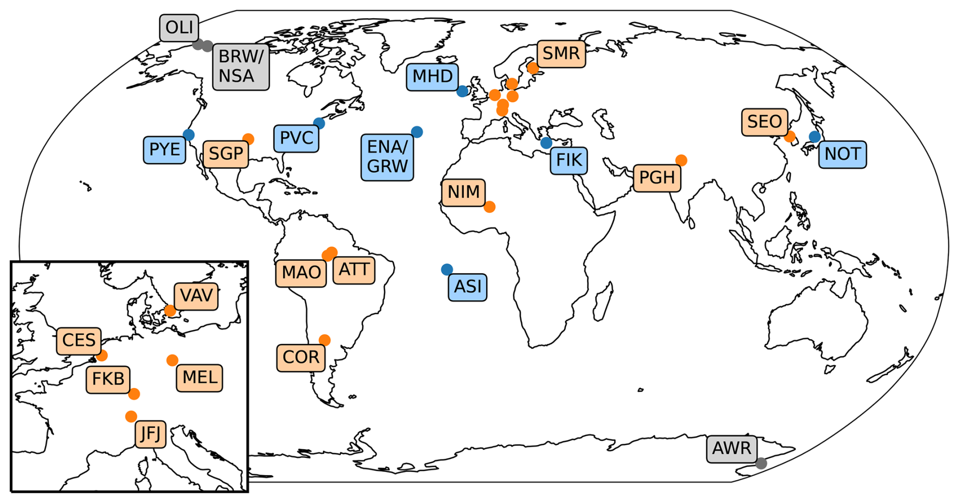
Figure 1 Locations of ground-based measurement sites. BRW and NSA as well as ENA and GRW share the same location, respectively. Continental stations in orange, marine in blue and polar stations in grey. The full station names, provided time periods and available supersaturations of each measurement site are listed in Table 1.

Table 1 Information on ground-based measurement sites that are used in this study. The given time frame indicates year and month of the first and last data point of the respective dataset of observations. The table contains a list of the supersaturations that are present in the given data files of each observation. For ARM stations, supersaturation setpoints are given. For SGP, four lists of supersaturations are provided, one for each available data product (AOSCCN, AOSCCNAVG, AOSCCN1COLAVG, AOSCCN2COLAAVG).

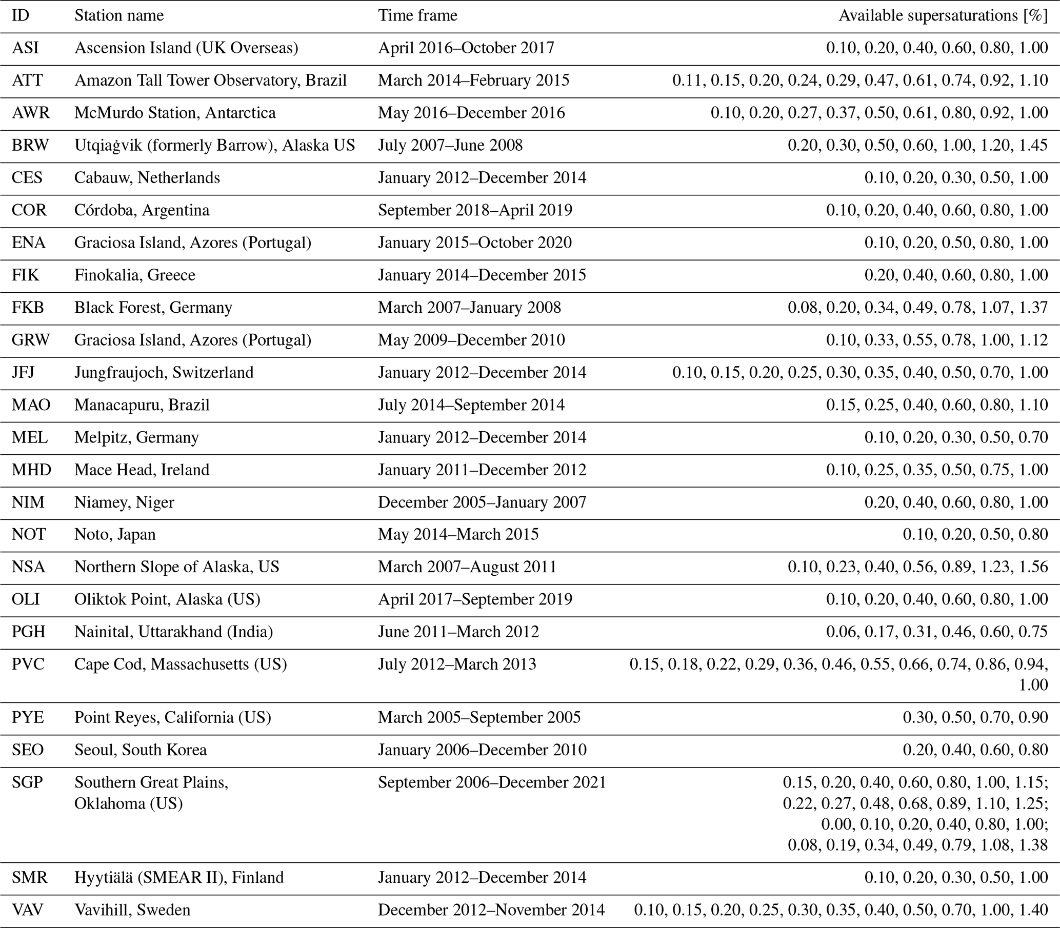
7 of these 25 stations are part of the European Aerosols, Clouds, and Trace gases Research InfraStructure (ACTRIS, http://www.actris.eu/, last access: 23 June 2026): Cabauw (CES), Finokalia (FIK), Jungfraujoch (JFJ), Melpitz (MEL), Mace Head (MHD), Hyytiälä (SMR) and Vavihill (VAV). Information about these stations as well as about the stations of Seoul (SEO) in South Korea, Noto (NOT) in Japan, Utqiaġvik (formerly Barrow, BRW) in USA and Amazon Tall Tower Observatory (ATT; Pöhlker et al., 2016) in Brazil are given in Schmale et al. (2017, 2018). At each of these 11 stations, a single-column CCN counter (model CCN-100) by Droplet Measurement Technologies (DMT; Roberts and Nenes, 2005; Rose et al., 2008) was used.

The remaining 14 datasets from Ascension Island (ASI), McMurdo Station (Antarctica, AWR), Córdoba (COR), Graciosa Island (ENA and GRW, covering two time periods), Black Forest (FKB), Manacapuru (MAO), Niamey (NIM), North Slope of Alaska (NSA, same location as BRW), Oliktok Point (OLI), Nainital (PGH), Cape Cod (PVC), Point Reyes (PYE) and Southern Great Plains (SGP) are provided by the United States' Department of Energy's Atmospheric Radiation Measurement (ARM, https://www.arm.gov, last access: 23 June 2026) user facility. Either single- or dual-column DMT CCN counters have been running at the ARM measurement sites and various data products were available at the time of this analysis. With the different data products, also varying levels of data quality checks were provided. The published data quality reports for each station (also see https://www.arm.gov/data/data-quality-program, last access: 23 June 2026) have been used to remove suspect, incorrect and missing data. Furthermore, the following criteria have been applied to all datasets in the process of data checking: There must not be more than one single file per day of measurement. This file has to contain a valid time dimension and no negative Nccn or supersaturation values. A list of all removed dates is given in Table A1 in the Appendix. The measurements from ENA and GRW (Graciosa Island), as well as those from BRW and NSA (north of Alaska), were taken at the same ARM facilities.

At SGP, four different data products are available for overlapping time periods (Fig. A1), which we combined to one time series. Between two data products, which are available for the same period, we have always selected that one with the higher reported level of data quality. Thus, the AOSCCN (Aerosol Observing System Cloud Condensation Nuclei) product covers the period from 13 September 2006 to 31 December 2010, AOSCCNAVG (AOSCCN Average) from 1 January 2011 to 31 October 2012, AOSCCN1COLAVG (AOSCCN Single Column Average) from 1 November 2012 to 16 August 2017 and AOSCCN2COLAAVG (AOSCCN Dual Column Average) from 17 August 2017 to 31 December 2021.

Following Spracklen et al. (2011) who assessed an uncertainty range in observed Nccn of 5 %–40 % depending on the magnitude of concentrations, supersaturation and the type of CCN instrument used, we assume a maximum relative uncertainty of ±40 % and a minimum absolute uncertainty of ±20 cm⁻³ in observed Nccn, as was done in Block et al. (2024).

2.3 Data treatment

Please note that in the remainder of this study, CCN_C refer to Nccn derived from CAMS and CCN_O are observed Nccn. Supersaturation is abbreviated as s. In order to validate CCN_C with observed data, we processed and homogenized both datasets. The model height level is chosen such that the geopotential height of the nearest grid point to the measurement site matches the measurement altitude approximately. To reduce representativeness errors associated with comparing point-based observations to gridded model output, a horizontal mean of the nine nearest CAMS grid points surrounding each measurement site was used. This spatial averaging mitigates the influence of sub-grid variability and small spatial displacement errors. Using only the nearest grid point resulted in systematically lower correlation coefficients (not shown).

As a last step of preparation, for some stations the CAMS-derived Nccn are normalized from ambient temperature and pressure (ATP) to standard temperature and pressure (STP). This is done by using the ideal gas law for standard conditions (T₀=273.15 K, p₀=1013 hPa), as e.g. in Holanda et al. (2020) and Andrews et al. (2025):

$$\begin{array}{}\text{(1)}& {\displaystyle }{\displaystyle }{\text{Nccn}}_{\text{STP}}={\text{Nccn}}_{\text{ATP}}\left({\displaystyle \frac{T_{\mathrm{0}}}{T}}{\displaystyle \frac{p}{p_{\mathrm{0}}}}\right).\end{array}$$

Observational data of BRW, CES, FIK, JFJ, MEL, MHD, NOT, SEO, SMR, and VAV are already given for STP conditions, while ATT data is normalized to STP using Eq. (1). Observed Nccn from ASI, AWR, COR, ENA, FKB, GRW, MAO, NIM, NSA, OLI, PGH, PVC, PYE, SGP are given for ATP conditions. Accordingly, CAMS-derived Nccn are compared to observations under the same conditions.

In the files from the ARM sites, two types of supersaturations are given: One setpoint supersaturation and one calculated supersaturation, which can differ significantly, as described in Andrews et al. (2025) and Lance et al. (2006). Here, the calculated supersaturation was chosen as it resembles the actual supersaturation in the flow chamber.

Since CAMS-derived Nccn are available only once per day at 00:00 UTC, we sub-sampled the corresponding observed data and computed medians and interquartile ranges of the hourly measured Nccn from 22:00 UTC to 02:00 UTC. We will refer to these medians as 00:00 UTC daily medians.

As mentioned, CCN_C are given at 6 specific supersaturations (s = 0.1 %, 0.2 %, 0.4 %, 0.6 %, 0.8 %, and 1.0 %). Observed Nccn are usually not measured at the same supersaturations. Therefore, CCN_O are directly taken (or averaged if several exist) within a range of ±0.05 %. In case there is no data in the ±0.05 % range, we interpolated linearly in the narrow range of ±0.1 %. The resulting uncertainties from this interpolation are small in comparison to the measurement uncertainties. However, not all supersaturations are covered at each measurement site, not even in a ±0.1 % range. To be able to interpolate across a wider range of supersaturations, we preferred a power law to a linear function. Nevertheless, we limit the inter-/extrapolation interval [s₁,s₂] to a maximum range of ±0.4 % around the desired value s_x, to reduce the inaccuracies, which are introduced by using a constant slope k across a range of supersaturations (see discussion in Sect. 2.4).

Thus, an Nccn value that is missing at a supersaturation s_x, but available at s₁ and s₂, is estimated by applying a power law to a given Nccn value at $s_i\in [s_{\mathrm{1}},s_{\mathrm{2}}]$:

$$\begin{array}{}\text{(2)}& {\displaystyle }{\displaystyle }\text{Nccn}\left(s_x\right)=\text{Nccn}\left(s_i\right){\left({\displaystyle \frac{s_x}{s_i}}\right)}^k,\end{array}$$

with the exponent k given from:

$$\begin{array}{}\text{(3)}& {\displaystyle }{\displaystyle }k={\displaystyle \frac{\ln \left(\frac{\text{Nccn}\left(s_{\mathrm{1}}\right)}{\text{Nccn}\left(s_{\mathrm{2}}\right)}\right)}{\ln \left(\frac{s_{\mathrm{1}}}{s_{\mathrm{2}}}\right)}},\end{array}$$

as it was derived e.g. in Block et al. (2024) and Désalmand (1985). Equation (2) is a generalized form of the power law proposed by Twomey (1959), which has been widely used for the approximation of CCN activation spectra (e.g., Martins et al., 2009; Andreae, 2009; Hudson, 1980; Cohard et al., 1998). Commonly, s_i is assumed to be 1.0 % and the power law is written as

$$\begin{array}{}\text{(4)}& {\displaystyle }{\displaystyle }\text{Nccn}\left(s_x\right)=\text{Nccn}\left(\mathrm{1}\mathrm{\%}\right)s_x^k,\end{array}$$

with a constant slope parameter k, that is independent of the desired supersaturation s_x.

2.4 Limitations to Twomey's power law

Several experimental and theoretical studies have pointed out that the simplicity of Twomey's power law comes with its limitations (e.g. Pöhlker et al., 2016; Deng et al., 2013; Ji and Shaw, 1998; Khvorostyanov and Curry, 2006; Cohard et al., 1998). Most importantly, it does not account for an aerosol-limited regime (e.g. Reutter et al., 2009) at high supersaturations, potentially leading to overestimated Nccn at high supersaturations. One reason is that the slope parameter k in Eq. (4) is assumed to be constant over the entire range of supersaturations; an assumption that has been contradicted by multiple observational studies (e.g. Kim et al., 2011; Khvorostyanov and Curry, 2006; Yum and Hudson, 2001). Instead, k has been shown to decrease with increasing supersaturation (Khvorostyanov and Curry, 2006; Cohard et al., 1998). The curvature of the activation spectrum depends on the size distribution of aerosol particles and thus, the environment of the respective air mass. Marine air masses with hygroscopic and bigger aerosol tend to have lower k values than continental environments, where small, hydrophobic particles are present (Jayachandran et al., 2020; Pruppacher and Klett, 1997). Cohard et al. (1998) stated that a power law with a constant k is not able to reproduce this curvature.

Several studies attempted to expand the original power law, e.g. using logarithmic (Wang et al., 2021) or exponential fits (Ji and Shaw, 1998). Khvorostyanov and Curry (1999) proposed a superposition of single-k power laws for different ranges of supersaturation and aerosol sizes, letting k decrease with increasing supersaturation and decreasing aerosol size.

In the following, we will show that using generalized s-dependent k parameters retrieved from observations give a very accurate representation of measured CCN spectra (Sect. 3.2) and are suited to be applied to simulated Nccn at one single supersaturation in order to create a full CCN spectrum.

2.5 Statistical approaches and analyzed parameters

The correlation between simulated and observed Nccn, as well as the quality of fit, are assessed using the bias B, the Pearson correlation coefficient R and, as a combined metric, the Kling–Gupta efficiency (KGE).

The relative bias B is computed from the medians of CAMS-derived and observed Nccn:

$$\begin{array}{}\text{(5)}& {\displaystyle }{\displaystyle }B={\displaystyle \frac{\text{med}\left({\text{CCN}}_{\mathrm{C}}\right)-\text{med}\left({\text{CCN}}_{\mathrm{O}}\right)}{\text{med}\left({\text{CCN}}_{\mathrm{O}}\right)}}\cdot \mathrm{100}\mathrm{\%}.\end{array}$$

A bias B of 0 corresponds to equal medians. Unless stated otherwise, the sign of the bias is kept and indicates overestimation (+) or underestimation (−). This means especially that an increasing B is not necessarily equal to a larger deviation of simulated to observed Nccn. It might as well indicate a transition from under- to overestimation. When averaging biases from a group of stations, the sign will be disregarded, which gives the absolute value $\left|B\right|$.

Following its standard definition, the Pearson R is

$$\begin{array}{ll}{\displaystyle }& {\displaystyle }R=\\ \text{(6)}& {\displaystyle }& {\displaystyle \frac{{\sum }_{i=\mathrm{1}}^n({\text{CCN}}_{\text{O,i}}-{\stackrel{\mathrm{‾}}{\text{CCN}}}_{\mathrm{O}})({\text{CCN}}_{\text{C,i}}-{\stackrel{\mathrm{‾}}{\text{CCN}}}_{\mathrm{C}})}{\sqrt{{\sum }_{i=\mathrm{1}}^n({\text{CCN}}_{\text{O,i}}-{\stackrel{\mathrm{‾}}{\text{CCN}}}_{\mathrm{O}}{)}^{\mathrm{2}}{\sum }_{i=\mathrm{1}}^n({\text{CCN}}_{\text{C,i}}-{\stackrel{\mathrm{‾}}{\text{CCN}}}_{\mathrm{C}}{)}^{\mathrm{2}}}}},\end{array}$$

with n being the number of points in the observation period.

The Kling–Gupta efficiency (KGE; Gupta et al., 2009) is a metric used to quantify the quality of a model's fit to observations and is widely used in hydrology. It is employed here to jointly account for bias (quantified by B) and explained variability (represented by R) and is defined as

$$\begin{array}{}\text{(7)}& {\displaystyle }{\displaystyle }\text{KGE}=\mathrm{1}-\sqrt{(R-\mathrm{1}{)}^{\mathrm{2}}+(\mathit{\alpha }-\mathrm{1}{)}^{\mathrm{2}}+(\mathit{\beta }-\mathrm{1}{)}^{\mathrm{2}}}.\end{array}$$

R is the Pearson correlation coefficient, $\mathit{\alpha }=\frac{{\text{std}}_{\mathrm{C}}}{{\text{std}}_{\mathrm{O}}}$ is the ratio of the standard deviations of CCN_C and CCN_O, $\mathit{\beta }=\frac{{\stackrel{\mathrm{‾}}{\text{CCN}}}_{\mathrm{C}}}{{\stackrel{\mathrm{‾}}{\text{CCN}}}_{\mathrm{O}}}$ is the ratio of the means of CCN_C and CCN_O. The higher a KGE value is, the better the fit is between observation and simulation. A maximum KGE of 1 is obtained for two perfectly matching datasets. Negative KGEs are possible but do not necessarily correspond to anti-correlating data or a certain sign of the bias. In this study, the KGE of each station is mainly used as a comparison metric and will always be related to other stations. An absolute statement, whether a certain number is considered high or low, will not be made.

Total median Nccn have been examined using the introduced metrics B, R, and KGE. These primary metrics are further distinguished for their spatial variability (e.g. accounting for environmental setting and pollution regime) and for their variability in time (e.g. accounting for seasonal differences).

The assessed spatial variability is based on a classification defining the environment at each station as either marine or continental. Sites that are located south of 70° S or north of 70° N (outside the CAMS assimilation range) are classified as a separate group of polar stations (Fig. 1).

Commonly, aerosol and CCN concentrations are also distinguished for different regimes. For example, Varghese et al. (2016) used a classification into clean (<1000 cm⁻³), polluted and highly polluted (>2000 cm⁻³), based on the Nccn at a supersaturation of 1 %. Andreae (2009) proposed a threshold of 600 cm⁻³ at 0.4 % supersaturation for polluted marine regions and Hudson and Yum (2002) defined groups of clean (<200 cm⁻³) and polluted air masses (>1000 cm⁻³) for 1 % supersaturation, with a transition regime in between. In this study, most analyses are based on 0.4 % supersaturation as a mid-range supersaturation level. At this supersaturation, a classification into a clean (${\text{CCN}}_{\mathrm{O}}<\mathrm{500}{\mathrm{cm}}^{-\mathrm{3}}$) and polluted ($\mathrm{500}{\mathrm{cm}}^{-\mathrm{3}}\le {\text{CCN}}_{\mathrm{O}}$) regime has been constructed, which is similar to the mentioned classifications by Andreae (2009) and Hudson and Yum (2002), but with lower thresholds than in Varghese et al. (2016).

Since one aim of this study is to validate the spectral behavior of CAMS-derived Nccn, the sensitivity of the Nccn to a change in supersaturation will be used as a secondary metric. These Nccn–s spectra are approximated by applying Twomey's power law. The slope of the spectrum is then described by the slope parameter k, using Eq. (3) for s₁=0.1 % and s₂=1.0 %. The larger k the steeper the activation spectrum is. Large k are usually found for continental or polluted air masses (Martins et al., 2009; Pruppacher and Klett, 1997).

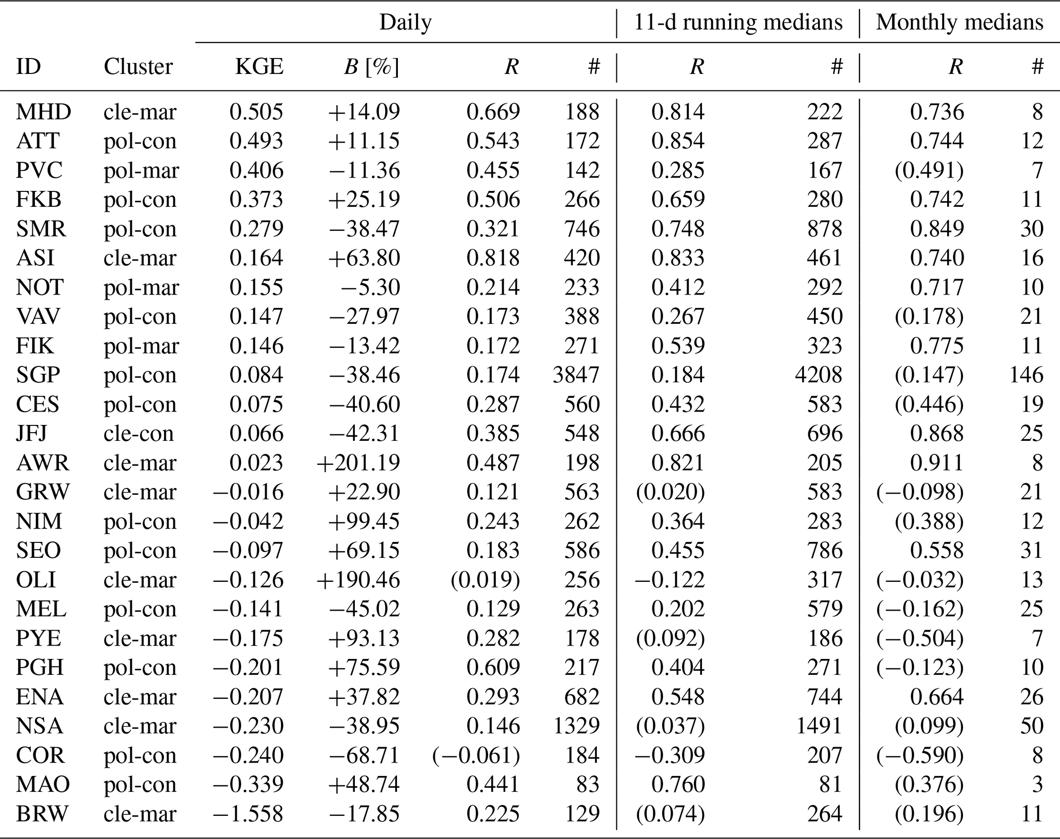
Table 2 Cluster (as defined by observed pollution regime and environment), Kling–Gupta efficiency KGE, bias B, correlation coefficients R and number of points # as derived from daily CAMS CCN data at 00:00 UTC and observational data from 22:00 UTC to 02:00 UTC for all 25 stations, sorted by KGE from highest to lowest. CCN are taken at s=0.4 %, except for ATT where s=0.4 % was not available as such and instead s=0.47 % was applied here – which eventually might lead to a slightly decreased bias. R values in parentheses indicate not significant correlations (95 % confidence interval). The cluster names are abbreviated: clean continental as “cle-con”, polluted continental as “pol-con”, clean marine as “cle-mar”, polluted marine as “pol-mar”. In comparison, correlations were also computed for 11-d running medians and monthly medians, both based on or around 00:00 UTC data only.

3 Results and discussion

3.1 The performance in time and space

Different environments and regimes certainly affect the order of magnitude of Nccn and thus the validity of CCN_C presented here. In order to compare different stations with each other we make use of the primary statistical quantities B, R, and KGE from daily data at or around 00:00 UTC and distinguish the stations by observed pollution regime and environmental setting. A summary is given in Table 2.

3.1.1 Evaluating the performance in time

Using the advantage of the CAMS-derived Nccn dataset as a continuous multi-year time series, a qualitative assessment of its ability to reproduce temporal variability is performed. Table 2 compares R values for each station distinguishing daily medians, running medians with windows of 11 d and monthly medians, all based on 00:00-UTC time periods.

Using daily 00:00-UTC medians, only 5 out of 23 stations with significant correlation coefficients show R values above 0.5 indicating at least moderate correlation of day-to-day fluctuations. This is a poor result considering that the CCN data are derived from a reanalysis in which the underlying aerosol fields are constrained by observations. Diurnal variations which might impact bias and correlation coefficient cannot fully be evaluated here only using 00:00-UTC CAMS data. Hence, applying 3-hourly CAMS CCN data could be very beneficial to account for these effects. However, in the current dataset by Block (2023), this temporal resolution is not available yet. A more detailed analysis on short-term variability of selected sites is given in Anders et al. (2025).

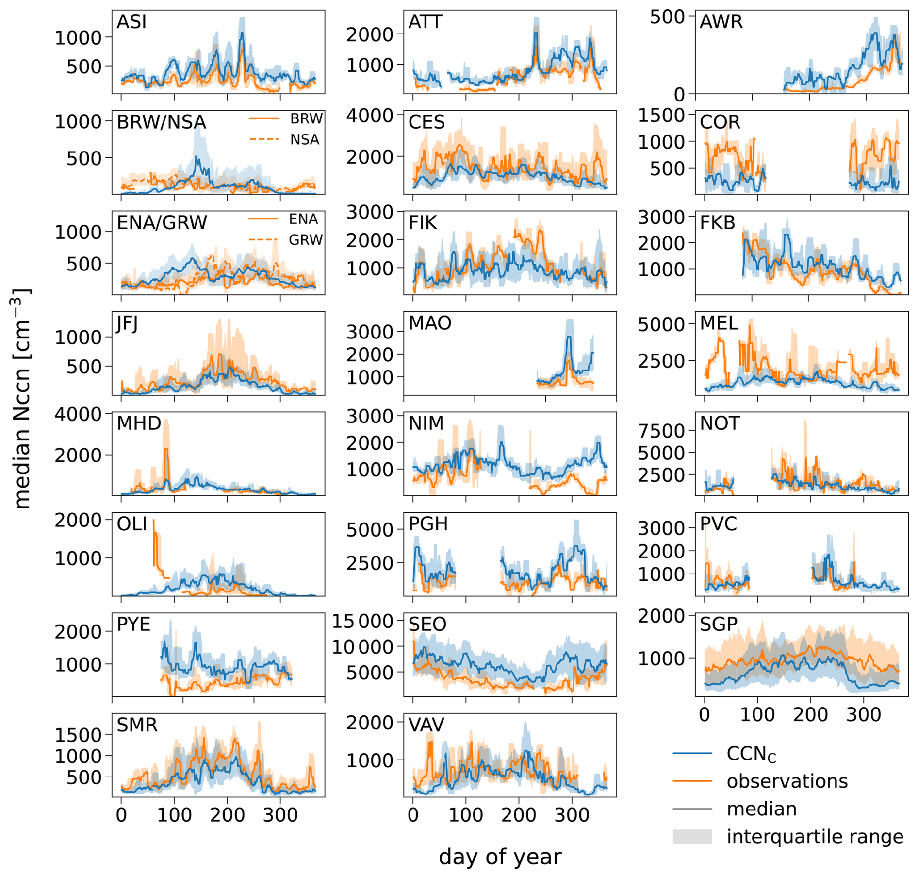
Figure 2 Climatologies for all stations at a supersaturation of 0.4 %. CCN_C in blue and CCN_O in orange, both with a running median and interquartile range in a window of 11 d. Please note: Data from 29 February has been removed and the co-located data from BRW and NSA as well as ENA and GRW are shown in the same tile.

Applying an 11-d running median on both datasets largely removes variability shorter than the synoptic scale, thereby improving temporal clarity of the time series at most stations. This filtering increases the correlation coefficient of 17 stations, compared to the daily medians, and thus, enhances the confidence that the CAMS-derived Nccn captures variability on synoptic time scales. Still, only 10 of 21 stations yielding significant result show R values larger than 0.5, which is about half of all stations. Correlation coefficients increase again for 8 stations when using monthly medians, especially for NOT, FIK and JFJ the increase is quite drastic. However, only for 11 of the 25 stations significant correlation coefficients are found. For those, R values range from +0.558 to +0.911 within all remaining 11 stations across all environments and pollution regimes.

The results of Table 2 are further illustrated in Fig. 2 showing multi-year 11-d running medians, and Fig. A2 showing multi-year monthly medians of Nccn (s=0.4 %) for all stations. Even though a correlation analysis of seasonal and annual medians does not produce significant results, as the available measurement periods are not long enough, we can visually judge the simulated temporal variability over several months indicating a yearly cycle from Figs. 2 and A2. From those 18 stations with at least 10 months of continuous observations available, 13 agree with CAMS in the yearly distribution of CCN, featuring e.g. correct differences in summer/wintertime CCN (SEO, SMR, SGP or JFJ), spring/autumn CCN (ATT, CES or FKB) or the double summer peak for VAV. Furthermore, at stations featuring wet and dry seasons, such as ATT, FIK, NIM and SEO (Pöhlker et al., 2016; Kouvarakis et al., 2000; Galy-Lacaux and Modi, 1998; Schmale et al., 2018), the increase in observed dry season Nccn is well captured by CAMS-derived Nccn (Fig. A3).

From this we conclude that CAMS-derived Nccn mostly reproduces the observed variability on monthly and seasonal time scales and therefore is suitable to be used for climatological applications and studies focusing on these timescales.

3.1.2 Dependencies on environment and pollution regime

There are no systematic differences in KGE at one fixed supersaturation (here 0.4 %), when comparing the four clusters. Averaging between all clean marine stations results in a KGE of −0.181, for polluted marine a KGE of 0.236, for clean continental 0.066 and for polluted continental stations 0.033. These differences are small compared to the spread between stations of the same cluster (Table 2). Furthermore, analyzing the KGE in dependence of the stations' geographical position or separately their environment or pollution regime has given no clear result either.

Block et al. (2024) made the comment, based on PGH data only, that very polluted sites might be overestimated by CAMS CCN. To further evaluate this feature we examined the bias of the most polluted sites available in our observations. Observations at SEO, MEL, CES, NOT, FIK and PGH all show median CCN_O>1000 cm⁻³ for s=0.4 %, outranging all other observations. But only SEO and PGH are overestimated by CAMS, while the other 4 stations are underestimated. Thus, we cannot confirm that heavily polluted sites are high biased in general. However, examining data from other megacities, such as in Asia and Africa, might be necessary, as our list of stations only included one (SEO).

For most stations, the pollution regime as identified by CCN_C (s=0.4 %) matches the regime it would have if regimes were defined by the observational CCN_O (s=0.4 %). A comparison of both definitions is part of Table A2. Only 4 stations deviate as a result of their bias, and thus would fall into a different category. Due to their negative bias, SMR, VAV and COR are classified in CCN_C as clean regimes instead of polluted ones. Meanwhile, PYE is classified as polluted instead of clean due its positive bias. A decrease in absolute bias would lead to a correction of pollution regime identification.

3.1.3 Polar sites

Four sites (AWR, BRW, NSA and OLI) lie in polar regions and therefore outside of the global domain of the data assimilation scheme of ECMWF's IFS between 70° S–70° N. Due to possible irregularities caused by the lack of observational constraints in this area, CAMS-derived Nccn data need to be used carefully. In particular, the co-located stations BRW and NSA exhibit simulation features that did not appear at any other station. There are partially sharp peaks, exceeding the observations by a factor of up to 4, and extremely low concentrations below 1 cm⁻³ in the winter months. These extremes result in very low correlation coefficients at both BRW and NSA. The same holds for the nearby station OLI. The Antarctic station AWR, however, exhibits a value of R that is comparable to stations of the mid-latitudes but it produces a very large bias (Table 2) even though, both CCN_O and CCN_C are very low. The presence of wrong peaks and large biases illustrates very clearly that the benefits of the assimilation of satellite observations are missing for the polar regions.

3.2 The CCN-supersaturation spectrum

3.2.1 Evaluating the CCN spectrum

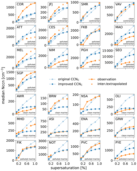
As depicted from Fig. 2, CCN are overestimated by CAMS at some stations (e.g. AWR, NIM or ASI), while underestimation is present at others (e.g. MEL, JFJ or SGP). These offsets change depending on the chosen supersaturation (Anders et al., 2025), as different fractions of CCN species get activated and thus shape the CCN spectrum.

Figure 3 compares observed and CAMS-derived Nccn-supersaturation spectra, which are computed from daily median Nccn for all six supersaturations, for which CAMS-derived total CCN are available. Both, CCN_C and CCN_O increase with supersaturation as expected. However, while CCN_O show shallower slopes for higher supersaturations, CCN_C grow almost linear with supersaturation and do not reach an aerosol-limited regime as the observations. Consequently, this leads to both an overestimation (positive bias B) at high supersaturations and an underestimation for low supersaturations. Table A2 summarizes nicely how biases evolve with supersaturation. While for s=0.1 % only 8 stations were positively biased but 17 stations had a negative bias, this reversed for s=1.0 %, where 19 stations had a positive bias but only 6 were negatively biased. For 20 out of 25 stations, B at a supersaturation of 1.0 % is larger (more positive or less negative) compared to its value at 0.1 %. When assessing how large the biases are in comparison, we need to look at their absolute values. 11 stations (of which 7 are marine) have larger $\left|B\right|$ at higher than at lower supersaturations, while 14 stations (of which 9 are continental) depict larger $\left|B\right|$ at low supersaturations. In the median of all stations, the absolute value $\left|B\right|$ is 65.89 % for s=0.1 % and 53.13 % for s=1.0 %. Hence, the underestimation at low supersaturations (which is reached more often in natural cloudy conditions) is an at least equally important issue as the overestimation at high supersaturations.

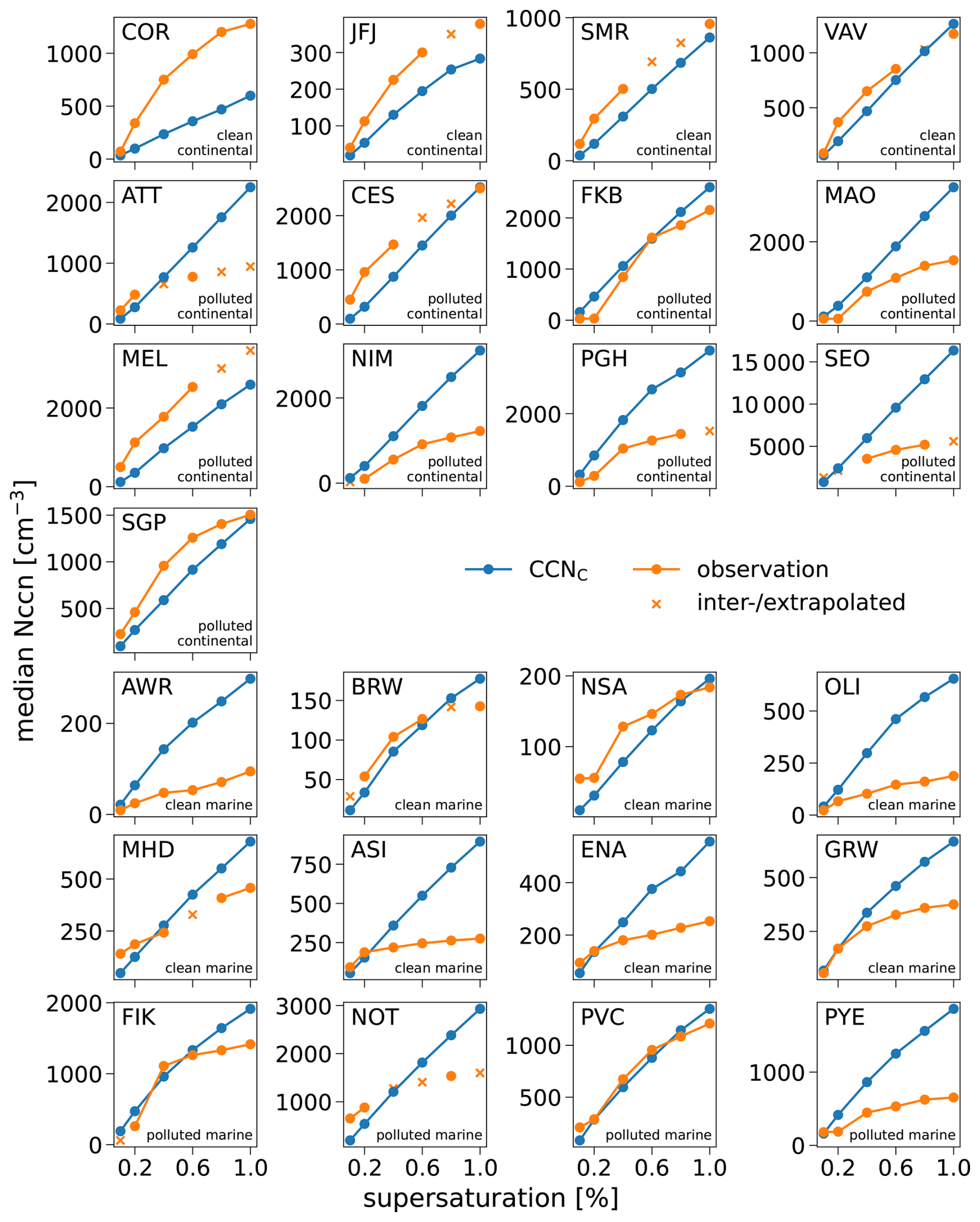
Figure 3 Nccn–s spectra showing the medians of every analyzed ground-based measurement campaign over the corresponding supersaturation. CCN_C in blue and CCN_O in orange. Observation values that are indicated by an “x” are medians of an inter- or extrapolated set of 00:00-UTC daily Nccn, using Twomey's power law (Eq. 2). Please note, the y axis is different in every plot. The x axis is shared.

As found by Anders et al. (2025), the best-fitting supersaturation s_best, for which B is closest to zero, differs between stations. As noted before and depicted in Fig. 4, marine stations are least biased at low supersaturations, while continental stations are least biased at higher supersaturations.

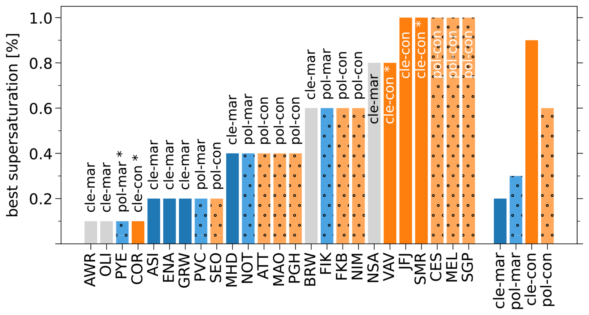
Figure 4 Supersaturation where CCN_C and CCN_O show best fit, for each station respectively. Distinguished into clean marine (“cle-mar”, blue), polluted marine (“pol-mar”, purple), clean continental (“cle-con”, green) and polluted continental (“pol-con”, orange) clusters, as defined by CCN_C. Cluster names with an asterisk indicate stations where the regime classifications of CCN_C and CCN_O do not match (see also Table A2). On the right, the respective median best supersaturation of each cluster. Polar stations are shown in grey for completeness but are excluded from the cluster median.

All three remote marine stations have their s_best at 0.2 % and, together with MHD, they create a “clean marine” category. The “polluted marine” category is dominated by coastal stations with mostly marine but also continental influence. These stations show a larger variability of s_best, ranging from 0.1 to 0.6, with a median value of s=0.3 %. Stations of the “polluted continental” category mostly occupy the larger supersaturation ranges around 0.6 %. A separate “clean continental” category emerges because CAMS-derived Nccn underestimates the pollution level at several inland stations (COR, VAV, and SMR). Without these classification mismatches, this category would contain only JFJ. This class has a median s_best at 0.9 %.

Some stations do not fit perfectly into this framework. For example, COR exhibits nearly identical biases for 1.0 % as for 0.1 % (Table A2) and is just by minimal deviations an outlier here. Because of a regime mismatch, similar holds for PYE, which would fit very well to the according cluster if it would actually be clean-marine as observed. However, because our objective is to correct the CAMS-derived dataset itself, all classifications are based on the aerosol regimes represented by CAMS rather than on observational categories. Finally, we find no systematic relationship between s_best and pollution regime alone. Instead, both environmental setting and pollution regime are required to explain the observed variability in s_best.

The curvature of a CCN spectrum depicted in Fig. 3 and thus the bias for each supersaturation might be dependent on the involved aerosol species. As already depicted in Block et al. (2024), Nccn derived from CAMS are mostly dominated by organic matter (OM) and sulfate (SO₄), while black carbon (BC) fractions are mostly small and the fractions of the three sea salt (SS) modes are negligible, even under remote marine conditions. With higher supersaturation, smaller and less hygroscopic aerosols get activated. Hence, the OM and BC fractions increase with supersaturation, while the portions of SO₄ and SS are reduced. Looking at the ratio of the OM and SO₄ fractions, we found a very clear relationship to the above-mentioned slope parameter k (Fig. 5): The larger the OM-to-SO₄ ratio, the larger is k. A logarithmic fit was found with an R² of 0.865. Large OM-to-SO₄ ratios above 1.5 at 0.2 % supersaturation are found at MAO, NIM and ATT. These three stations indeed exhibit similar shapes in Fig. 3, having a strongly increasing B with increasing supersaturation. On the other hand, stations with low OM-to-SO₄ ratios (FIK, AWR and BRW), below 0.3 at 0.2 % supersaturation, tend to have a weaker increase in B. It seems that the stations with lower OM fractions are likely to have a smaller absolute value $\left|B\right|$, but tend to produce a lower correlation coefficient R. As a result of these two contradictory effects, a systematic relation of the OM-to-SO₄ ratio on the KGE could not be determined. Examining the sea salt and BC fractions, no significant correlation to the KGE is obtained either.

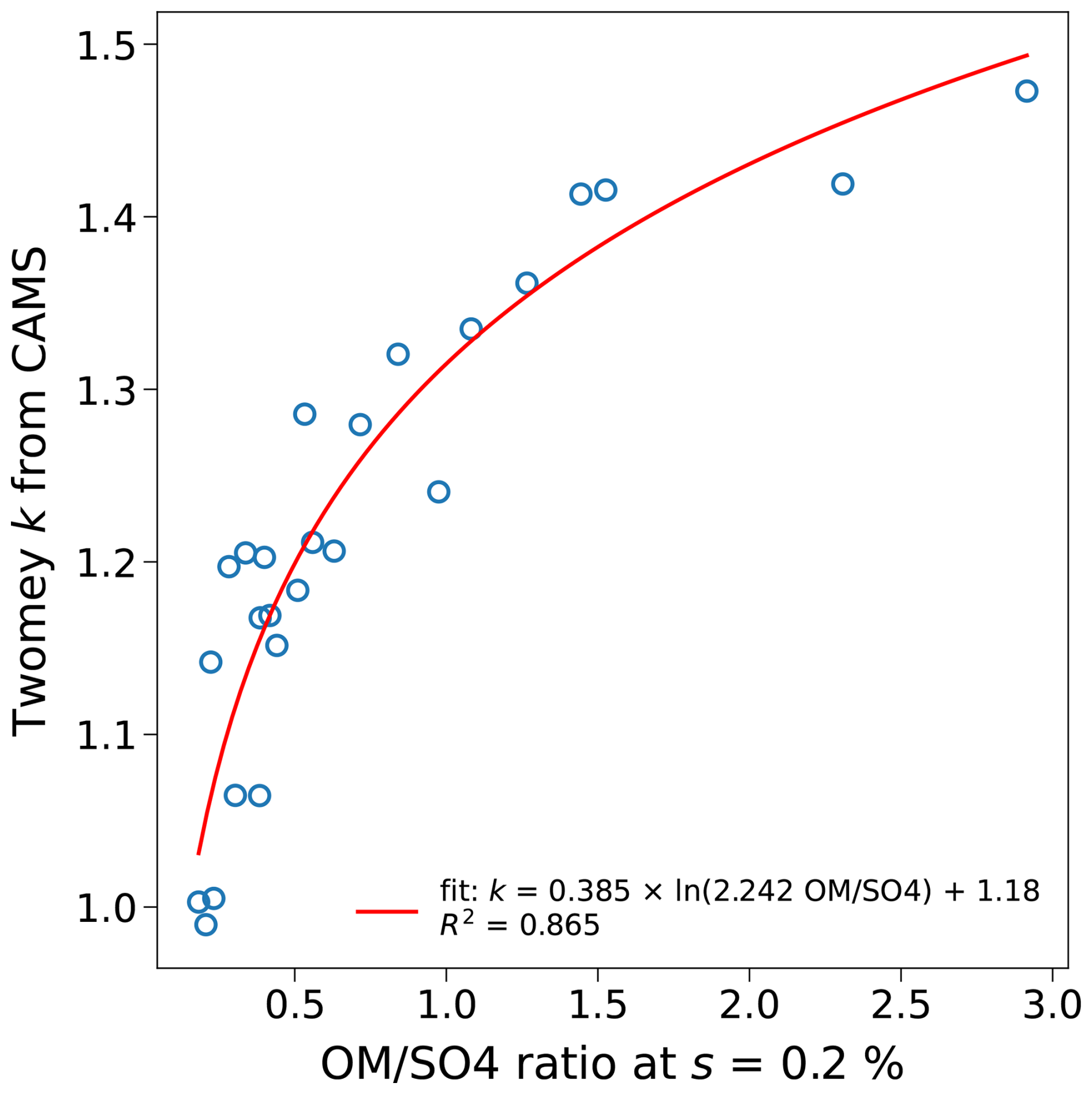
Figure 5 Slope parameter k from CCN_C, as defined by Eq. (3) with s₁=0.1 % and s₂=1.0 %, against the ratio of the median organic matter (OM) and sulfate (SO₄) CCN_C fractions. Each data point (blue circle) represents one station. A logarithmic fit was performed (red solid line).

This specific feature suggests a possible cause of the biased CCN spectrum. The discrepancy could stem from uncertainties in the emission fractions of CCN-relevant aerosol species (as these are not constrained in CAMS), from limitations in the assumed aerosol size distributions and composition used in the CCN calculations (e.g. fixed global modes and kappa values, assumption of external mixtures), or from a combination of both. Nevertheless, the overall Nccn spectrum may be improved without modifying aerosol size distributions or species concentrations. Instead, this approach relies solely on the observed CCN spectrum as demonstrated in the following section.

3.2.2 Deriving a spectral k(s) from observations

As described in the previous section, we found large biases in CAMS-derived Nccn at both low and high supersaturations. To reduce these biases, we present an approach tailored to the unique characteristics of the CAMS-derived Nccn dataset. The idea is to fit the simulated Nccn–s spectrum to the observations. For that, due to its simplicity and its prevalent application in CCN activation spectra (e.g. Martins et al., 2009; Cohard et al., 1998), we use Twomey's power law (Eq. 4). However, its original form must be modified to serve the targeted purpose, reducing biases in CCN_C at both low and high s.

First of all, we cannot use 1.0 % as the reference supersaturation s_i, since this would preserve the large biases at this supersaturation. Instead, we use a cluster-specific reference, which accounts for the different s_best we found in the previous section for the different clusters (Fig. 4). Based on these findings, we defined four cluster-specific s_i: 0.2 % for clean marine, 0.4 % for polluted marine, 0.6 % for polluted continental sites and 1.0 % for clean continental stations.

Generalizing Twomey's power law by applying it to other supersaturations than 1.0 % has been done already (e.g. Block et al., 2024; Andreae, 2009) and in our case, it is a promising modification to avoid high-supersaturation biases and to target each environment specifically. It needs to be noted that this flexibility in particular is the main advantage of the power law over other parameterizations. The exponential function by Ji and Shaw (1998), the error function by Pöhlker et al. (2016) and the logarithmic formulation by Wang et al. (2021) all have Nccn (1.0 %) as one of their inputs. We do not want to evaluate the capabilities of all these parameterizations for fitting observed Nccn–s spectra here as they are not suitable for our purpose.

Figure 6 The slope parameter k(s), derived from the observations (Eq. 3) and grouped by clusters identified by CAMS-derived Nccn. Polar stations are excluded.

Furthermore, we found for our data that keeping a constant exponent k in the power law leads to increased biases at low supersaturations. Similar results have been shown e.g. by Kim et al. (2011) and Wang et al. (2021). Furthermore, k derived from observations decrease with supersaturation (e.g. Khvorostyanov and Curry, 2006; Cohard et al., 1998; Yum and Hudson, 2001). This is also the case for the majority of observations we use in this study: Fig. 6 depicts k values of each station, as calculated from Eq. (3). For this and the following other k parameterizations, we use Nccn medians of the full daily cycle that is available in the observations (not limited to the period between 22:00–02:00 UTC as for the analysis above). We do this to increase the robustness and confidence in our improvements of CAMS-derived Nccn.

We propose to use these observation-derived, spectral k(s) instead of a constant k in the power law:

$$\begin{array}{}\text{(8)}& {\displaystyle }{\displaystyle }\text{Nccn}\left(s_x\right)=\text{Nccn}\left(s_i\right){\left({\displaystyle \frac{s_x}{s_i}}\right)}^{k\left(s\right)}.\end{array}$$

Similar notations of a power law with a supersaturation-dependent exponent have been used by e.g. Khvorostyanov and Curry (2006, 2008), and Liu et al. (2011). For the purpose of reducing low supersaturation biases in CCN_C and ultimately, simulating a more accurate CCN activation spectrum, this approach is suitable to modify the yet too steep slope of the CCN_C spectrum.

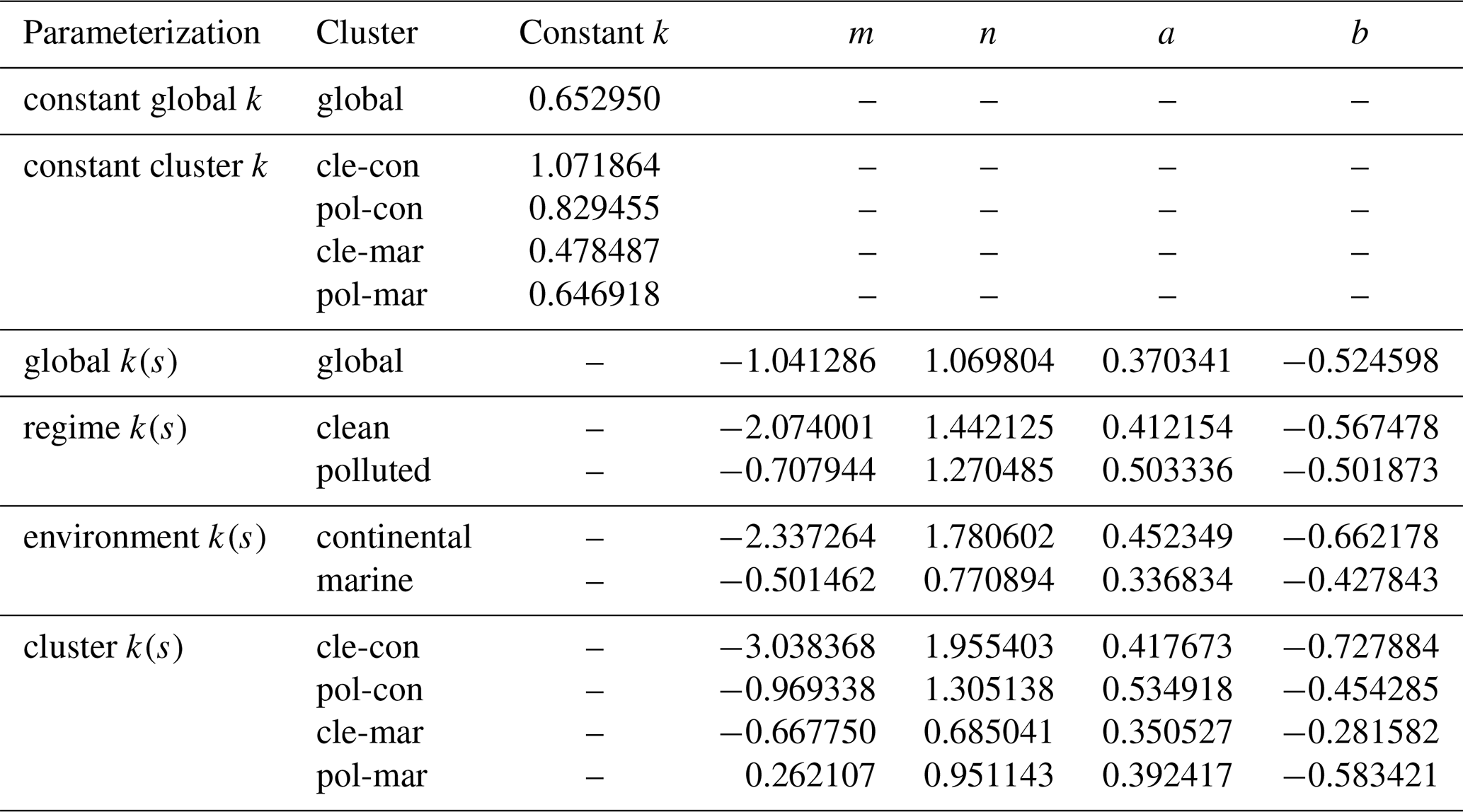
As a first step, we average the calculated station-specific k(s), to obtain a global spectrum. Since the majority of stations we use are continental, calculating the median across all stations would result in a bias towards the continental stations. Thus, we group the observation-derived k(s) spectra of the stations by environment and compute the median of both groups. To account for the uneven global distribution of continental (30 %) and marine environment (70 %), we perform a weighted average of these environment medians for each supersaturation, to obtain a global spectrum of observation-derived k(s). At the six CAMS supersaturations, the values are 0.838, 0.727, 0.669, 0.464, 0.455, and 0.436, respectively. For comparison, we calculated the same global, environment-weighted mean k(s) from CCN_C which gives 1.312, 1.162, 1.099, 1.006, 0.952, and 0.868, respectively. It becomes clear that the observation-derived k(s) differ widely from an analogously CAMS-retrieved k(s), revealing the root of the biased CAMS-derived CCN spectrum.

Lastly, to reduce the risk of overfitting to our set of observations and to extrapolate k(s) to 0.1 % and 1.0 %, we applied a power law fit for supersaturations starting at 0.2 % and a linear fit extrapolating to 0.1 %. The power law appears to be the best-fitting function for the given points of k(s). The second linear fit is necessary due to the nature of the power law, which would grow to infinity at low values of s. Similarly, Khvorostyanov and Curry (2006) have found observed k spectra to decrease more slowly in the range below 0.12 % supersaturations compared to higher s. Wang et al. (2021) used a piecewise function that fits Nccn below 0.1 % linearly, which gives better results than the Twomey parameterization.

The global k(s) parameterization can be written as:

$$\begin{array}{}\text{(9)}& {\displaystyle }{\displaystyle }k\left(s\right)=\left\{\begin{array}{lr}-\mathrm{1.041286}s+\mathrm{1.069804}& \text{for }s<\mathrm{0.2}\mathrm{\%}\\ \mathrm{0.370341}{s}^{-\mathrm{0.524598}}& \text{for }s\ge \mathrm{0.2}\mathrm{\%}\end{array}\right\}.\end{array}$$

We also explored other possible derivations of a k–s spectrum, by treating each regime/environment/cluster individually instead of a global mean. In Fig. A4, we show a comparison of these approaches at SMR, SGP, ENA and FIK, which are the stations with the highest number of points in their respective cluster.

For the constant k parameterizations, we apply Eq. (3) with s₁=0.1 % and s₂=1.0 % for each individual station, resulting in one single-value k per station. For applying a correction with a constant global k, we group these k values by environment and perform a weighted average of the median of all continental stations (30 % weight) and median of all marine stations (70 % weight). Thus, we use one single-value k globally. The correction with a constant cluster k is done similarly but with grouping by cluster before applying the median single-value k in the respective cluster.

Additionally, bias corrections are performed with four different k(s) parameterizations in comparison. First, an s-dependent spectrum of k(s) is calculated for each station. For applying a correction using a global mean k(s) on all stations, we group these station spectra by environment and perform a weighted average of the median of all continental stations (30 % weight) and median of all marine stations (70 % weight). The resulting global average k(s)-spectrum is fitted, as described above. Thus, we use one global k(s)-spectrum for each station. The parameterization with a regime dependent k(s) is done by grouping the station spectra by regime and fit the regime-median k(s). This fitted spectrum is used for each station of the respective regime. Parameterizations using the environment dependent k(s) and the cluster dependent k(s) are done similarly, but by grouping first by environment or by cluster, respectively.

All Nccn parameterizations are then retrieved from Eq. (8) with the respective k or k(s) and the cluster-specific reference supersaturation s_i (clean continental: 1.0 %, polluted continental: 0.6 %, clean marine: 0.2 %, polluted marine: 0.4 %.)

For most stations the differences between group-specific (regime, environment, cluster) and global k(s) are not very large (as at ENA and FIK in Fig. A4), thus it would be unnecessary to distinguish between clusters (or environments/regimes), as we did for the definition of s_i. This simplifies applications on a global scale in any future developments or use cases. However, another reason why we prefer the parameterization with a globally weighted mean k(s) is that the bias correction produces the most balanced biases for low and high supersaturations, as can also be seen in Fig. A4 for SMR and SGP. Please note that all 25 stations behave differently, which is why the chosen parameterization is not necessarily the best fit at each station. It is rather a tradeoff between the individual stations and the applicability on a global scale. For completeness, all group-specific k(s) parameterizations are listed in Table A3.

3.2.3 Towards an improved CCN spectrum

Applying Eq. (9) to the six supersaturations CAMS-derived Nccn are available at, we receive a global spectrum of k(s) values, which are independent of the environment. Using the new global set of s-dependent k values and the environment-specific s_i, we applied Eq. (8) to the original daily CCN_C (s_i). The resulting medians are depicted in Fig. 7, which illustrates the improvement this new approach achieved. The curvature of the activation spectra at most stations is simulated more accurately. Especially, at the clean marine stations ASI, ENA and GRW as well as polluted marine FIK and NOT, this is the case. In addition, ATT, MAO, NIM, PGH and SEO are examples from the polluted continental cluster where high supersaturation biases are reduced significantly. However, Nccn which the original CCN_C have already underestimated (e.g. for CES, COR, JFJ, MEL, SGP) do not benefit from the adjustments and negative biases at continental stations and high supersaturations are enhanced. To account for these very region-specific biases, a modification of the underlying size distribution for CAMS-derived Nccn or a redistribution of CCN-relevant aerosol masses might still be necessary.

Figure 7 Same as Fig. 3, but with the addition of improved CCN_C (dark blue).

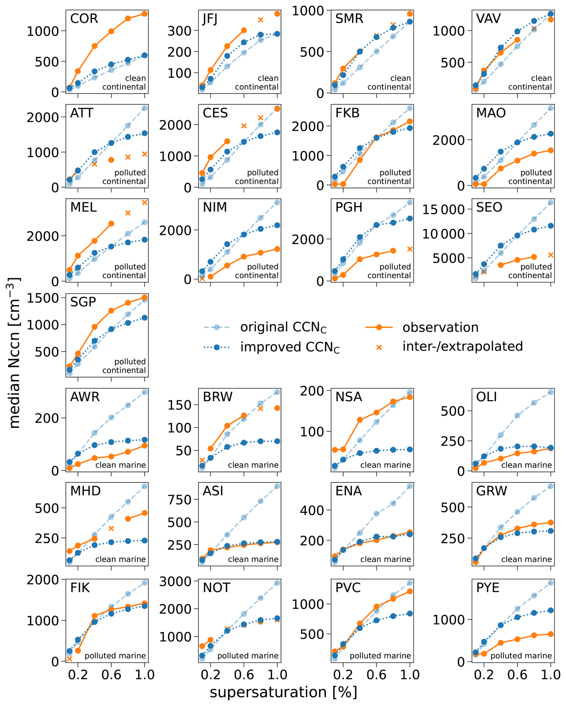
Despite these remaining challenges, we could reduce the biases for the majority of all stations (Fig. A5 in the Appendix). Especially at the high supersaturations 0.8 % and 1.0 %, the absolute values of the bias are decreased substantially. Also at low supersaturations, absolute biases $\left|B\right|$ are reduced in both environments. Specifically, the medians of the biases of all non-polar stations at 0.1 %, 0.2 %, 0.4 %, 0.6 %, 0.8 %, and 1.0 % supersaturation are reduced by 30.1 %, 29.5 %, 41.4 %, 34.5 %, 51.7 %, and 43.3 %, respectively. The improved median absolute values $\left|B\right|$ are 42.9 %, 36.8 %, 22.6 %, 26.1 %, 26.6 %, 30.1 %, respectively. Unlike Fig. A5, these absolute values do not indicate a direction of the bias (under-/overestimation) but show that we could reduce the magnitude of the biases at all supersaturations substantially.

4 Summary and conclusions

The recently published 3D-dataset of CCN number concentrations (Nccn) derived from CAMS reanalysis aerosol mass mixing ratios (Block et al., 2024) is evaluated against direct observations from 25 ground-based measurement sites. The evaluation focuses on three aspects of the CAMS-derived total Nccn: (1) its ability to reproduce observed temporal variability, from day-to-day fluctuations over synoptic-scale variations to monthly timescales; (2) its suitability across different environments (marine, continental) and pollution regimes (clean and polluted); and (3) its sensitivity to supersaturation.

Regarding temporal variability, performance varies substantially between stations, even within the same environment or pollution regime. In particular, the representation of day-to-day variability differs considerably across sites, with significant Pearson correlation coefficients ranging from +0.121 to +0.818. Only 5 of the 23 stations with statistically significant correlations at the 95 % confidence level exhibit correlation coefficients exceeding 0.5, indicating limited skill in reproducing daily variability despite the underlying aerosol fields being constrained by reanalysis data. However, model performance improves markedly as the temporal aggregation period increases. The highest correlation coefficients are obtained for monthly median values, with R ranging from +0.558 to +0.911, within all 11 stations still yielding statistically significant correlations. In addition, the CAMS-derived Nccn generally reproduces the observed seasonal cycles, including the occurrence of dry and wet seasons, at most stations yielding long enough continuous measurements. These results suggest that the dataset is well suited for climatological applications and studies focusing on monthly to seasonal timescales, while caution is warranted when interpreting day-to-day variability.

Considering the suitability of CAMS-derived Nccn in different environments and regimes, we evaluated Nccn for a mid-range supersaturation of s=0.4 % and made use of Kling–Gupta efficiency (KGE) as an estimate of quality of fit, taking into account correlation as well as bias. The resulting values show a large spread between stations and no clear dependence of the model's performance to environmental settings nor to pollution regimes. Investigations of the most polluted sites could not confirm the statement in Block et al. (2024) that there might be a tendency for overestimation at heavily polluted sites, even though we find that PGH and SEO are high biased. However, apart from SEO, we did not investigate data from other megacities. It should further be noted that CAMS-derived CCN data are indeed problematic in Arctic and Antarctic regions as large biases and low correlation coefficients are obtained at some of the investigated polar stations. This could be due to the lack of constrainment by the CAMS data assimilation scheme which is only active between 70° S–70° N. As already stated in Block et al. (2024), one should be careful when using the CAMS-derived CCN dataset in these regions.

The examination of the sensitivity of Nccn to different levels of supersaturation revealed an increasing bias with increasing supersaturations. At several stations, this results in a transition from underestimation at low supersaturations to overestimation at higher supersaturations. The bias shift could be described using the slope parameter k of Twomey's power law, which was applied onto the CCN-supersaturation spectrum. For almost all stations, CAMS-derived Nccn exhibit a larger k than observed Nccn, which is related to an overly steep activation spectrum. Further analysis suggests that these discrepancies are linked to the ratio of organic matter (OM) to sulfate (SO₄) of the related CCN species. Stations characterized by lower OM-to-SO₄ ratios generally exhibit smaller k values, implying a weaker supersaturation dependence. This points to potential deficiencies in the assumed aerosol composition and/or size distributions used in the derivation of the dataset. Consequently, refinements of the underlying size distribution may further improve the agreement with observations. While such modifications were beyond the scope of the present study and remain a topic for future dataset development, we instead developed an observation-based parameterization to address this issue. We demonstrate that its application to CAMS-derived total Nccn improves agreement with observations without modifying aerosol size distributions or species concentrations. These improvements further enhance the suitability of the CAMS CCN dataset for global aerosol-cloud-interaction studies.

A significant reduction of the biases in CAMS Nccn could be achieved by applying a modified power law with an s-dependent k spectrum, which has been derived from the observations. For the application on CAMS data we grouped the data into classes, distinguishing environmental settings (marine/continental) and pollution regimes (clean/polluted) for which we computed the least biased level of supersaturation. Thus, we find that e.g. marine stations are least biased at low supersaturations, while continental stations are least biased at higher supersaturations.

At a supersaturation of 1.0 %, the median bias decreased by 43.3 % to an absolute value of 30.1 %, indicating a reduction of the overestimation. For lower supersaturation of 0.1 %, it decreased by 30.1 %, to an absolute value of 42.9 %, which corresponds to a reduction of the underestimation at this supersaturation. The majority of stations exhibited more accurate re-presentations of their CCN-supersaturation spectra, especially those in marine environment. However, biases at high supersaturations persist at some stations.

Despite our efforts of exploring and evaluating CAMS-derived Nccn, further investigations should also focus on the validation of the vertical distribution, as some problems have already been addressed by Kulkarni et al. (2025) and Anders et al. (2025). It is also of importance to investigate the quality of CAMS-derived Nccn over yet neglected regions in Africa, Asia and Australasia and above the Southern ocean, since this study could only partially contribute to the discussion started by Choudhury et al. (2025). Additionally, the comparison to more stations of long-term CCN measurements over multiple years will help in assessing the representation of not only day-to-day but also annual variability and eventually multi-decadal trends.

Appendix A

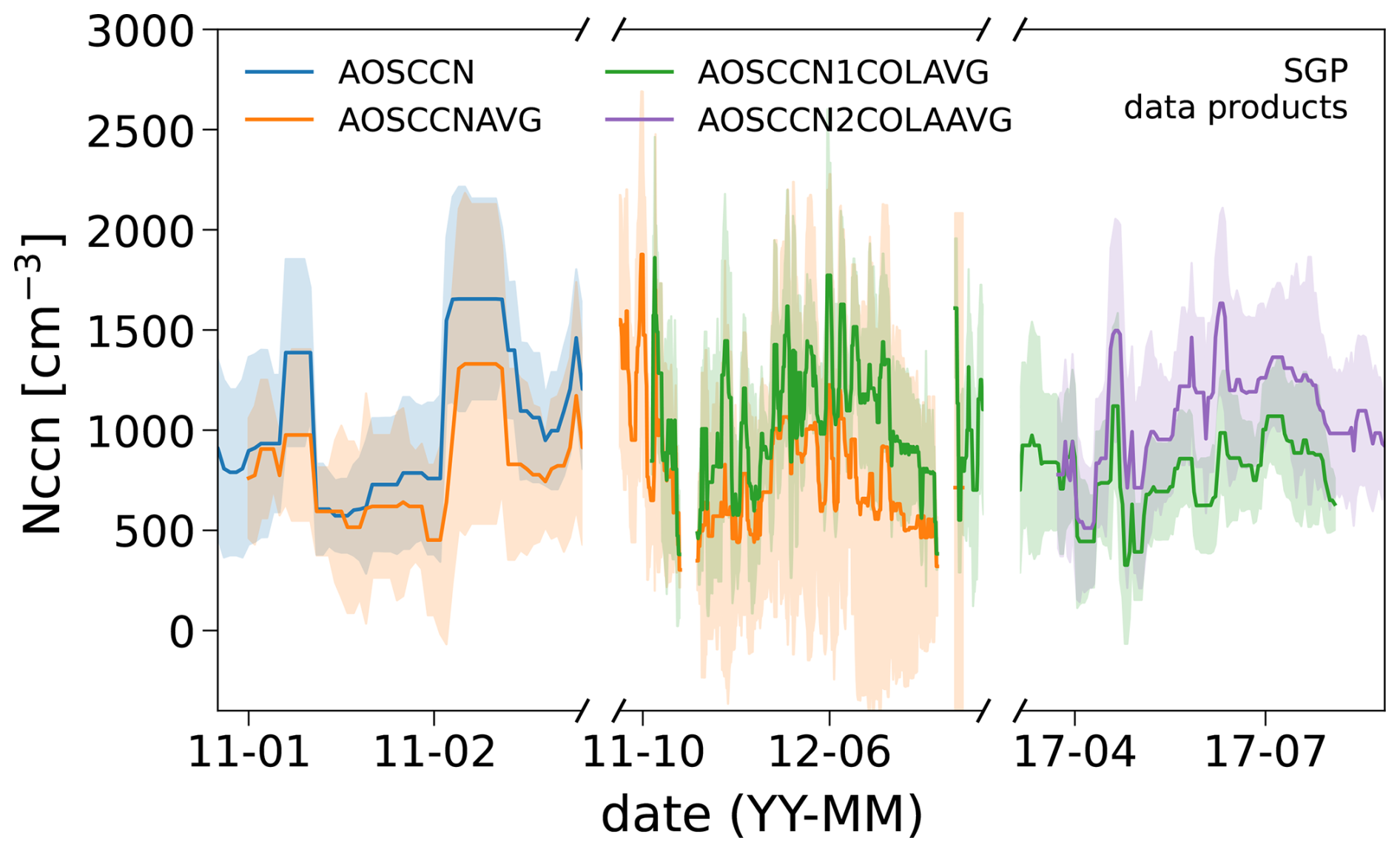
Figure A1 Periods of overlap of four data products of SGP that were available for our analysis: AOSCCN is the Aerosol Observing System Cloud Condensation Nuclei product, AOSCCNAVG is the AOSCCN Average product, AOSCCN1COLAVG is the AOSCCN Single Column Average product and AOSCCN2COLAAVG is the AOSCCN Dual Column Average product. We have combined these data products to one dataset, which we have used for this study. For overlapping time periods, we have selected that one with the higher reported level of data quality. Full-day Nccn are shown at 0.4 % supersaturation and with a 11-d running median and interquartile range.

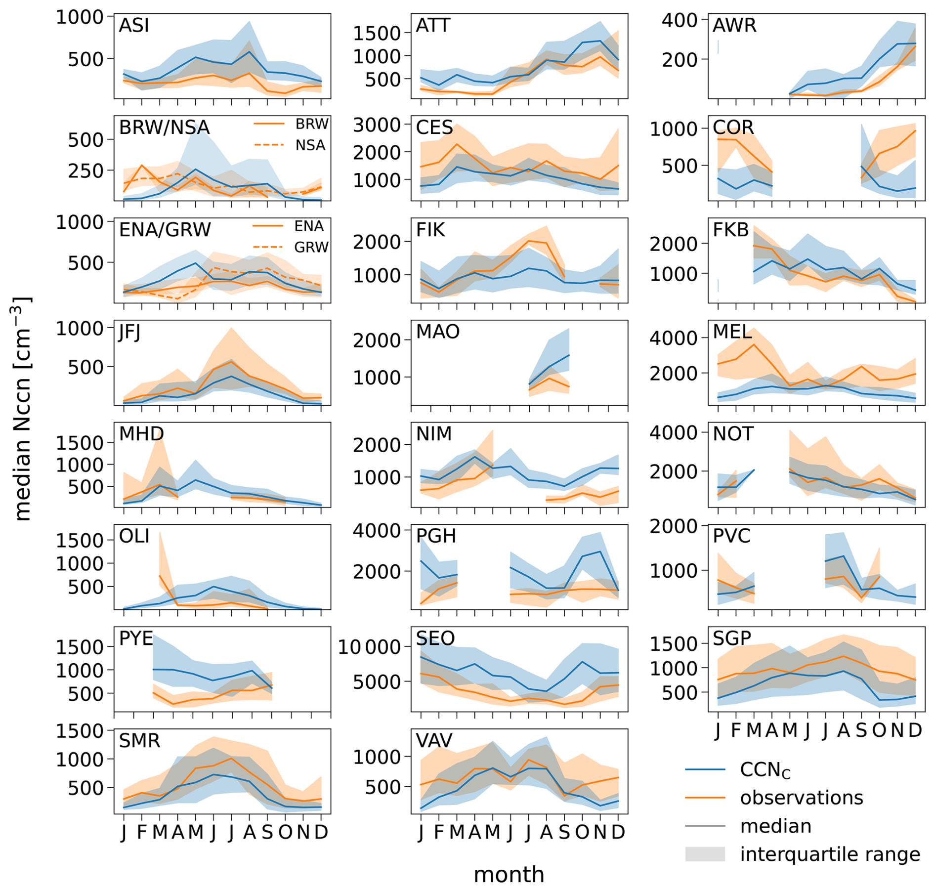
Figure A2 Climatologies for all stations at a supersaturation of 0.4 %. CCN_C in blue and CCN_O in orange, both showing monthly medians and interquartile ranges of 00:00-UTC daily values. Please note: The co-located data from BRW and NSA as well as ENA and GRW are shown in the same tile.

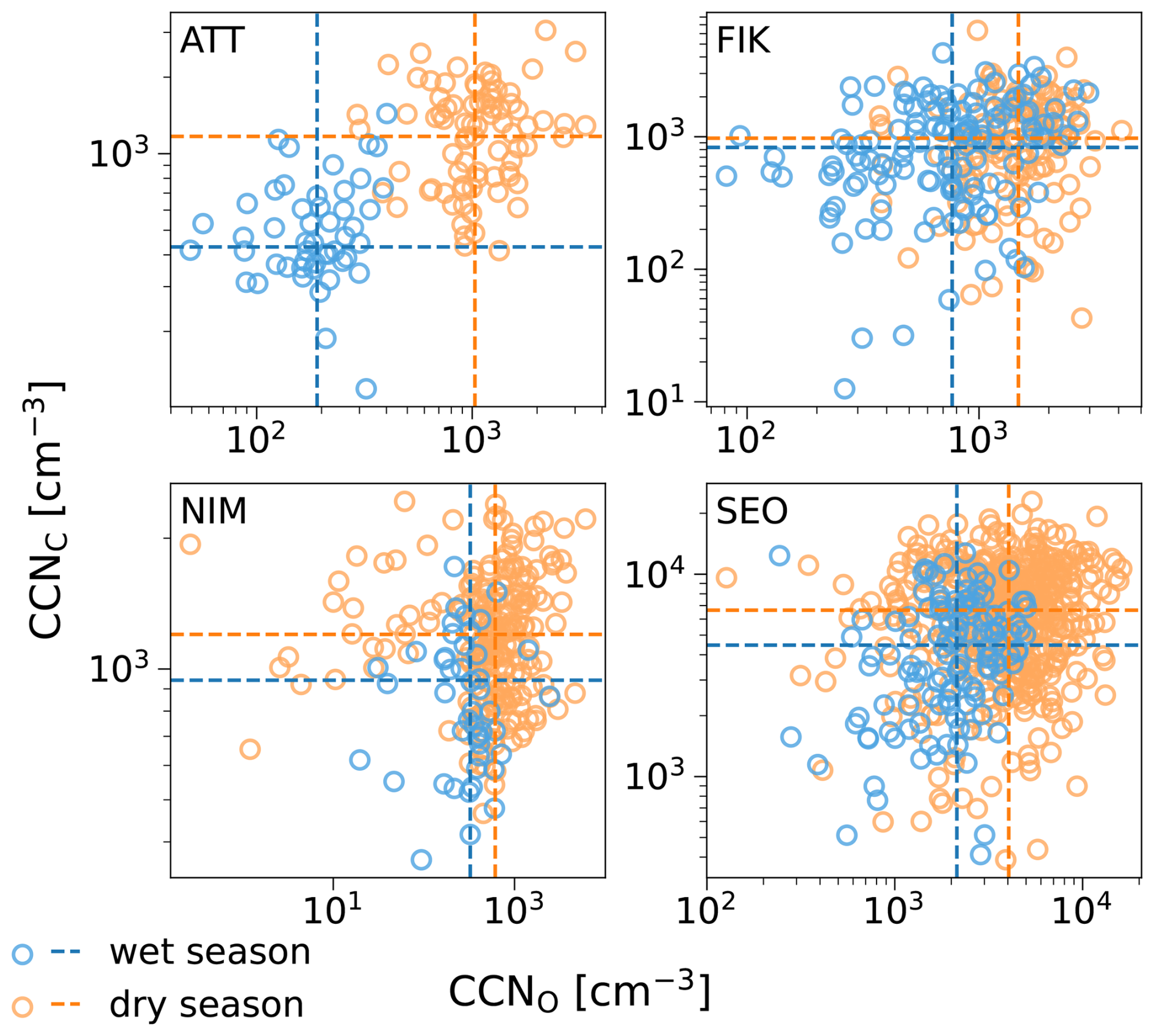
Figure A3 00:00-UTC median Nccn at ATT, FIK, NIM and SEO. Days of wet season periods in blue, dry season in orange. Season medians shown as dashed lines. Please note, all tiles have different axis ranges.

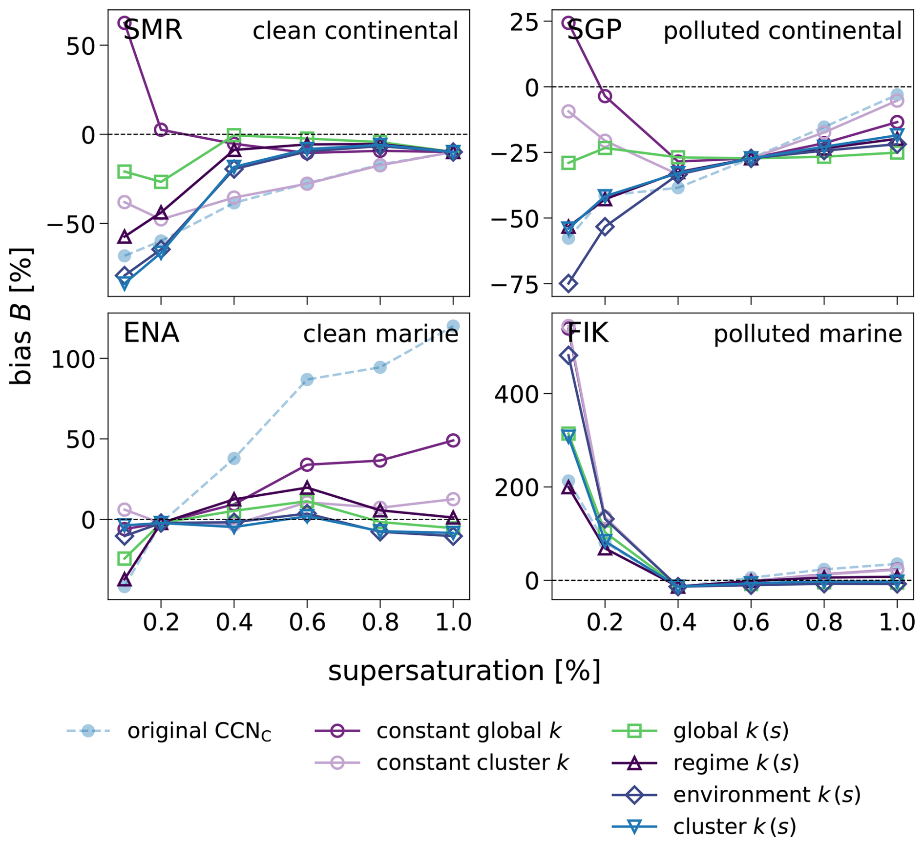
Figure A4 B–s spectrum at the SMR, SGP. ENA and FIK, showing the bias over the corresponding supersaturation for different parameterizations using the observation-derived slope parameter k. Please note, the y axis is different in each tile, the x axis is shared. We excluded the polar stations from the derivation of k and k(s). For the constant k-parameterizations, we apply Eq. (3) with s₁=0.1 % and s₂=1.0 % for each individual station, resulting in one single-value k per station. (1) Constant global k is a weighted mean of environment dependent k values. (2) Constant cluster k represents the median k derived from each cluster and applied to the respective cluster. Then for each station, we use the median of the single-value k in their respective cluster. For the s-dependant parameterizations, we calculate k(s) for each station. (3) Global k(s) is a weighted mean of environment dependent k(s) values. (4) The regime k(s) represents the fitted median k(s) derived for each pollution regime and applied to all stations of that regime. (5) Similarly, the environment k(s) represents the fitted median k(s) fore each environment, respectively, while (6) the cluster k(s) represents the fitted median k(s) for each cluster, respectively. All Nccn parameterizations are then retrieved from Eq. (8) with the respective k(s) and the reference supersaturation s_i (clean continental: 1.0 %, polluted continental: 0.6 %, clean marine: 0.2 %, polluted marine: 0.4 %).

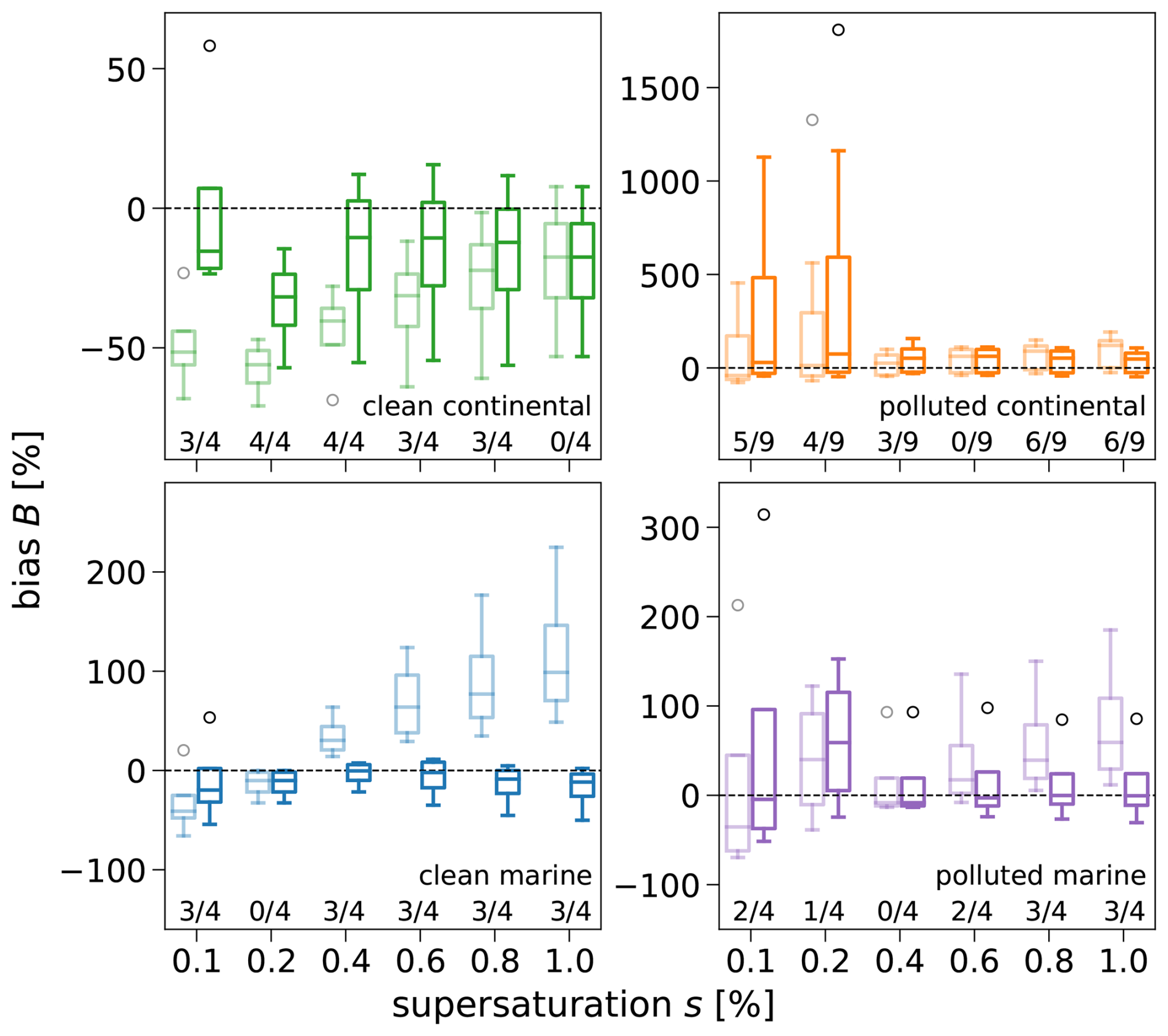
Figure A5 Statistics of the bias B at each supersaturation, depicted for clean continental (green), polluted continental (orange), clean marine (blue) and polluted marine (purple) cluster. Polar stations are excluded. CAMS-derived Nccn in light hue and the improved new CCN_C in dark hue. Each box plot includes the biases of all stations of the respective cluster and supersaturation. The numbers below show how many stations of the total in this category exhibit smaller absolute values of their bias after the improvement. Please note, the y axis is different in each tile, the x axis is shared and outliers are indicated by black circles.

Koontz et al. (2016b)Koontz et al. (2016a)Koontz et al. (2018)Koontz et al. (2015)Enekwizu et al. (2005a)Andrews et al. (2007)Koontz et al. (2017a)Enekwizu et al. (2006)Flynn et al. (2011)Koontz et al. (2011)Koontz et al. (2017b)

Table A1 References to observation data and removed files during data checking. Please note: This table does not list missing files, but only the removed files during the process of data checking.

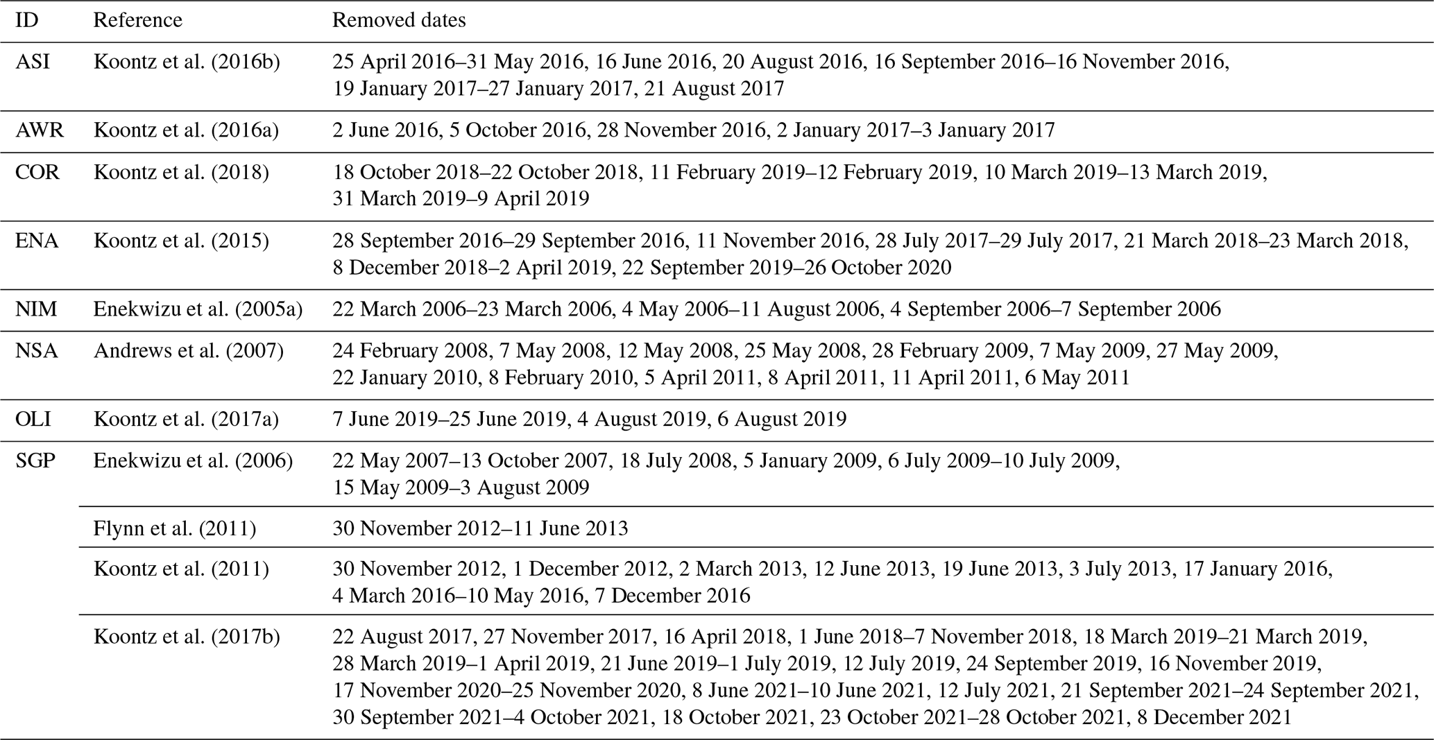
No dates needed to be removed for: ATT (Pöhlker et al., 2016) and BRW, CES, FIK, JFJ, MEL, MHD, NOT, SEO, SMR, VAV (Petäjä et al., 2017), and FKB (Enekwizu et al., 2007), PYE (Enekwizu et al., 2005b), GRW (Shilling and Kulkarni, 2009), MAO (Flynn et al., 2014), PGH (Shilling and Kulkarni, 2011), PVC (Shilling and Kulkarni, 2012).

Table A2 Regime, environment and for all 25 stations. The regime is derived from the 0.4-%-supersaturation median of (a) CCN_O and (b) CCN_C. Check marks indicate matching regimes in CCN_O and CCN_C. Furthermore, biases B [%] at at all six supersaturations s are shown, sorted by the best supersaturation at each station. The respective best bias is printed in bold font.

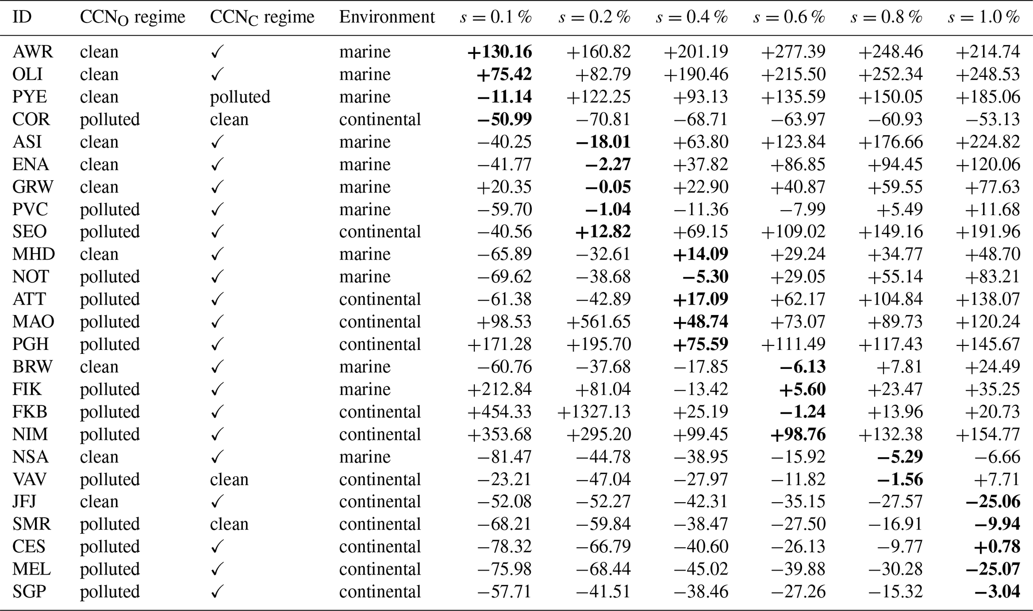
Table A3 Coefficients of the parameterizations we explored to improve the CAMS-derived Nccn spectrum. Cluster refers to the group of stations the respective parameterization should be applied to. A constant k is only given for parameterizations which rely on a single k value. The coefficients m and n are parameters of the linear function to fit the supersaturation range below 0.2 %: $k\left(s\right)=ms+n$. The coefficients a and b are parameters of the power function to fit the supersaturation range at and above 0.2 %: k(s)=a s^b. Thus, m, n, a, and b are only given for spectral k(s)-parameterizations.