Leveraging leaf-level optimality processes with explicit acclimation improves global GPP representation in an individual-based DGVM (LPJ-GUESS v4.1.1)

Vegetation models are indispensable tools for investigating and projecting the terrestrial carbon cycle, both as standalone models and embedded in global climate models. However, current models vary widely in their representation of ecosystem processes and consequently in their projected future carbon dynamics. Eco-evolutionary optimality (EEO) approaches, which derive and test hypotheses about optimal plant behaviour under specific environmental conditions as a consequence of natural selection, have been proposed as a means to improve the reliability of vegetation models and the robustness of their future projections. Here we embed EEO-derived models for photosynthesis and leaf dark respiration, and their acclimation to changing conditions, into the widely used LPJ-GUESS vegetation model. We evaluated the simulated gross primary production (GPP) patterns against remotely-sensed GPP derived from sun-induced fluorescence and found that the EEO configurations improved the spatial distributions (a mean reduction in error of 15 % across gridcells) and global interannual variability (a mean reduction in error of 32 % after accounting for differences in global totals) compared to the standard version of LPJ-GUESS. Evaluation against GPP fluxes from eddy flux covariance measurements also showed improved performance, the R² of 5 d GPP increased from 0.45 to 0.48 (averaged across 147 sites). The simulated global carbon pools, fluxes, burnt area and biome distributions were not impacted substantially. The improvements were achieved with no alteration to processes except photosynthesis, respiration and plant water uptake, and with no recalibration or tuning. The EEO configuration also reduced model run time and eliminated the need for poorly-constrained PFT-dependent parameters governing the temperature response of photosynthesis. As well as being a tangible improvement to LPJ-GUESS, this study further confirms the usefulness of EEO approaches to improve global vegetation models.

1 Introduction

Aggregated terrestrial photosynthesis, known as gross primary productivity (GPP), is a major flux in the global carbon cycle (Anav et al., 2015). Only about half of the carbon fixed by photosynthesis is used to produce biomass (Collalti et al., 2020), and a large proportion of the remainder is respired to support maintenance of tissues (Atkin et al., 2015). The photosynthetic apparatus in leaves is particularly costly to maintain, and leaf maintenance respiration, referred to here as leaf dark respiration (R_d), is estimated to use around 25 % of GPP (Piao et al., 2013; Ren et al., 2024). Understanding the response of these large carbon fluxes to environmental conditions is pivotal for understanding and simulating Earth system dynamics (Lombardozzi et al., 2015), especially given the strong coupling between the atmosphere and the biosphere.

Models of the terrestrial biosphere, including dynamic global vegetation models (DGVMs) and land surface models (LSMs), typically simulate GPP and R_d as part of their terrestrial carbon cycle. Although there is some shared ancestry between such vegetation models, they make different assumptions about the mechanisms controlling GPP and R_d, and different choices about the number of plant functional types (PFTs) they use and their associated parameter values. Whilst the models usually reproduce the present day spatial patterns of GPP reasonably well, they show very divergent patterns of carbon uptake by the biosphere under future climate change projections (Arora et al., 2020) reflecting a lack of understanding of the controls on these basic processes (De Kauwe et al., 2014; IPCC, 2023; Prentice et al., 2015). Most models simulate photosynthesis using the Farquhar, von Caemmerer and Berry (FvCB) biochemical model (Farquhar et al., 1980) or the modified version proposed by Collatz et al. (1991, 1992), both of which require three parameters: V_cmax, the maximum carboxylation rate; J_max, the maximum electron transport rate; and c_i : c_a, the ratio of leaf-internal to external CO₂ concentration, χ. Although the FvCB biochemical model (or Collatz variant) is common across vegetation models, they take different approaches to defining these parameters. They also take different approaches to modelling R_d. Many models treat dark respiration as a temperature dependent process, assume that this is proportional to V_cmax at a fixed temperature (usually 25 °C) and treat this as a constant per PFT and model the temperature dependence of Rd and V_cmax with separate Arrhenius equations (Crous et al., 2022). However, some models consider respiration as a function of the available carbon substrate pool or consider the requirements for maintenance and growth separately (Atkin et al., 2017).

Photosynthesis and dark respiration respond to environmental conditions on two different timescales. On short timescales (i.e. near instantaneous), V_cmax, J_max and R_d respond to changes in temperature as they are governed by enzyme kinetics. Over longer timescales (days to weeks) plants optimize their photosynthetic capacities, dark respiration and stomatal behaviour to changing environmental conditions through acclimation (Kumarathunge et al., 2019; Reich et al., 2016, 2021; Smith et al., 2019; Smith and Dukes, 2013). The representation of acclimation in current vegetation models is limited. Some models do not represent thermal acclimation (e.g. Krinner et al., 2005; Niu et al., 2011), while those that do use represent thermal acclimation using empirical functions and PFT-specific parameters derived from databases of plant trait measurements (Atkin et al., 2015; Kattge and Knorr, 2007) but using different timeframes ranging e.g. from the last 10 d or current monthly mean (Butler et al., 2021; Haverd et al., 2018; Huntingford et al., 2017; Mercado et al., 2018; Oliver et al., 2025; Vuichard et al., 2019). Models that include acclimation to changing temperature do not consider acclimation to other drivers such as atmospheric CO₂ concentration, [CO₂] (Bagley et al., 2015; Sage et al., 1989; Tissue et al., 1993), radiation (Atkin et al., 1998; Ghannoum et al., 1997; Liu et al., 2024), and VPD (Li et al., 2018; Middleby et al., 2024).

The Lund-Potsdam-Jena (LPJ-) DGVM (Sitch et al., 2003) and related models like LPJ-GUESS (Smith et al., 2014) adopt a somewhat different approach for calculating V_cmax and R_d. In this case an optimal daily V_cmax is calculated based on the assumption that plants optimise the net leaf-level photosynthetic gain, i.e. GPP−R_d, for a given daily temperature, radiation, daylength and [CO₂]. An additional temperature-response of photosynthesis is included according to an empirically-derived unimodal response function, with fixed (and poorly constrained) parameters for tropical, temperate and boreal PFTs (Sitch et al. 2003). R_d is linearly related to V_cmax so is also adjusted daily. Whilst this formulation allows plants to adjust their photosynthetic capacity and R_d according to temperature, it is not a reasonable representation of acclimation as the timescale of this adjustment (1 d) is unrealistically short.

Eco-evolutionary optimality (EEO) approaches have been suggested as a means to improve the vegetation models and enable more robust predictions by improving the representation of ecosystem processes and reducing the reliance on poorly constrained parameters (Harrison et al., 2021). EEO theory assumes that processes are optimised by natural selection and proposes concrete hypotheses about plant behaviour in response to environmental conditions. EEO hypotheses focus on predicting optimal plant function given environmental conditions, whilst acknowledging that plants do not immediately achieve this optimum but rather will adjust their functioning towards the predicted optimum at an appropriate time scale – i.e. they explicitly account for acclimation. This time scale varies from days-to-weeks for ecophysiological processes, to millennia or longer for evolutionary processes. A further advantage of EEO approaches is that they are based on equations derived from hypothesised plant behaviour rather than empirical relationships, and so they are innately well-suited to represent the broad spectrum of plant behaviour and dynamic traits, without discretising vegetation into PFTs with fixed trait values.

The P-model (Prentice et al., 2014; Stocker et al., 2020; Wang et al., 2017) is a universal model of GPP which combines three EEO hypotheses (the least cost hypothesis, the coordination hypothesis and the cost-benefit hypothesis for J_max: see Materials and Methods) and the FvCB model of C₃ photosynthesis. It simulates responses of photosynthesis to temperature, solar radiation, vapour pressure deficit, [CO₂] and atmospheric pressure. The standard version of the P-model (P model v1: Stocker et al., 2020) uses weekly or monthly climate inputs and so implicitly includes acclimation of ecophysiological processes on a weekly-to-monthly timescale. The sub-daily version of the P-model (Mengoli et al., 2022), which was explicitly designed for incorporation in LSMs, separates the instantaneous and acclimated response of photosynthesis to temperature where the acclimated response was determined from noontime conditions over a period of ∼15 d (Mengoli et al., 2022). A similar acclimation timescale has been identified for leaf dark respiration (Ren et al., 2024). Ren et al. (2025) have incorporated both the sub-daily P-model and an EEO-based scheme for R_d that represents the adjustment of leaf respiration to nighttime temperature and the coupling of V_cmax with canopy level R_d into the Noah-MP LSM. They showed that overestimation of GPP (10 %) and canopy respiration (200 %) in the standard version of the Noah-MP model compared to observed values at eddy covariance flux sites was substantially reduced (GPP: 2 % overestimation; canopy respiration: 8 % overestimation), pointing to the utility of adopting these schemes in vegetation models.

In this study we test the applicability of EEO-derived representations of leaf-level processes, including explicit representation of acclimation, in LPJ-GUESS (Smith et al., 2001, 2014). LPJ-GUESS is a widely-used, community-developed DGVM, which has also been implemented as an LSM in a number of climate models (Döscher et al., 2022; Forrest et al., 2020; Weiss et al., 2014). Our focus here is to go beyond the site-scale study with prescribed absorbed radiation and vegetation types of the Noah-MP study global implementation (Ren et al. 2025) by testing globally and with fully prognostically calculated light absorption and simulated vegetation dynamics. Specifically we (i) implemented the P-model and a complementary representation of leaf dark respiration in LPJ-GUESS, (ii) compared the simulated global GPP with a remotely-sensed GPP product based on sun-induced fluorescence (SIF), (iii) compared simulated GPP with measurements from eddy flux covariance sites and (iv) evaluated the effects of the new implementation on simulated global carbon pools and fluxes, water fluxes and the distribution of vegetation types.

2 Materials and methods

2.1 LPJ-GUESS (Lund-Potsdam-Jena General EcoSystem Simulator)

LPJ-GUESS (Smith et al., 2001, 2014) integrates processes ranging from ecophysiology and tree population dynamics to biogeochemical cycles, global vegetation biome changes, disturbances by wildfires and (in specific versions, not here) land use. The processes described in this section are enabled for all simulations presented here, unless specifically mentioned as modified or disabled for the EEO version of the model. Vegetation dynamics are simulated as the emergent outcome of growth and competition for light, space and soil resources (here nitrogen and water) among woody plant individuals and a herbaceous understorey in each of a number of replicate patches representing “random samples” of each simulated locality or grid cell. These replicate patches differ due to the stochastic processes of establishment, mortality and disturbance, and so represent landscape heterogeneity driven by succession dynamics. The simulated plants are classified into one of a number of Plant Functional Types (PFTs) discriminated by growth form, phenology, photosynthetic pathway (C₃ or C₄), bioclimatic limits for establishment and survival and, for woody PFTs, allometry and life history strategy. These traits determine which PFT competes most successfully in a given environment and, thereby, the relative cover of each PFT. Here we used the standard global PFTs set with ten tree PFTs and two herbaceous PFTs following Smith et al. (2014).

LPJ-GUESS's existing photosynthesis scheme follows the approach of LPJ-DGVM (Sitch et al., 2003), with the addition of a nitrogen limitation on photosynthetic rates following (Smith et al., 2014). Canopy fluxes of CO₂ and water vapour are calculated by a coupled photosynthesis and stomatal conductance scheme based on the approach of BIOME3 (Haxeltine and Prentice, 1996a, b). The scheme first calculates optimal photosynthesis in the absence of water stress by calculating the V_cmax which maximises net photosynthesis after accounting for leaf dark respiration (i.e. GPP−R_d) assuming fully open stomata i.e. $\mathit{\chi }={\mathit{\chi }}_{\max }=\mathrm{0.8}$. R_d is calculated as a fixed fraction of V_cmax. This V_cmax is used to calculate the unstressed photosynthesis and the corresponding transpirational water demand (via the requisite canopy conductance and the Priestly-Taylor representation of evapotranspiration). This demand is then compared to the water supply through roots from the soil to determine if the plant is water stressed. If this is the case, and the canopy conductance is down-regulated until the demand matches the supply, which also reduces χ and photosynthesis. Water supply here was calculated using LPJ-GUESS's default water update take scheme (referred to as “ROOTDIST”) which calculates supply as the product of plant root-distribution-weighted soil moisture and a maximum transpiration rate (5 mm d⁻¹). In this water uptake scheme, plant water availability is not limited by soil moisture content until the wilting point is reached, at which point available water is zero.

Nitrogen limitation is introduced to LPJ-GUESS's standard photosynthesis calculation as a scalar on V_cmax before any consideration of water stress (i.e. at the calculation of unstressed photosynthesis above). The scalar is the ratio of current photosynthetically-active leaf N content to the optimal leaf nitrogen. The latter is calculated based on unstressed V_cmax following (Haxeltine and Prentice, 1996a) and the former depends on soil N availability and the individual's uptake strength which depends on root surface area (Smith et al., 2014).

After subtracting respiration costs, the net primary production (NPP) accrued by an individual woody plant or the herbaceous layer each simulation year is allocated to leaves, fine roots and, for woody PFTs, sapwood, following a set of allometric relationships for each PFT, resulting in biomass, height and diameter growth (Sitch et al., 2003). Population dynamics (recruitment and mortality) are represented as stochastic processes, influenced by current resource status, demography and the life history characteristics of each PFT (Hickler et al., 2004). In the global standard version here, vegetation-stand-destroying disturbances are simulated as a stochastic process, affecting individual vegetation patches with an expectation of 0.01 yr⁻¹, which very roughly mimics natural disturbances such as tree diseases, storms and bark beetle attacks. In addition, wildfires are modelled prognostically using the SIMFIRE model (Knorr et al., 2014) with fire emissions and mortality calculated with the BLAZE model (Rabin et al., 2017) and are enabled in all simulations presented here. Litter arising from phenological turnover, mortality and disturbances enters the soil decomposition cycle. The carbon and nitrogen soil decomposition dynamics are jointly simulated using a scheme adapted from the CENTURY model (Parton et al., 1993). The soil hydrology scheme follows Gerten et al. (2004) which includes interception, infiltration, and percolation, and was recently updated to use 15 soil layers (Zhou et al., 2024).

2.2 The P-model

The P-model v1.0 (Stocker et al., 2020) combines an optimality-derived light-use efficiency (LUE) prediction with the Farquhar–von Caemmerer–Berry model for C₃ photosynthesis (FvCB). The LUE prediction is based on three EEO hypotheses. The Coordination Hypothesis (Chen et al., 1993; Haxeltine and Prentice, 1996a; Maire et al., 2012) assumes that plants equalise their RuBisCo-limited rate of photosynthesis (V_cmax) and their electron-transport limited rate of photosynthesis (limited by both J_max, the maximum rate of electron transport, and absorbed light) under growth conditions on a weekly-to-monthly timescale to optimise the use of available light. The Least Cost Hypothesis (Prentice et al., 2014) states that plants minimise the sum of the costs per unit assimilation for maintaining their apparatus for photosynthesis and transpiration. The Cost-Benefit Hypothesis for J_max (Peng et al., 2020; Wang et al., 2017) posits that plants optimise their J_max so as to maximise the net benefit i.e. the benefit to their assimilation rate minus the cost of maintaining their electron transport chain. Predictions for V_cmax, J_max, and χ (the ratio of leaf intercellular CO₂ concentration to atmospheric CO₂ concentration) are derived from these assumptions and used to calculate gross assimilation rates using the FvCB model (Stocker et al., 2020; Wang et al., 2017). The P-model v1.0 also includes a temperature-dependent quantum yield of photosynthesis, φ₀, and an empirical soil moisture limitation factor which was calibrated from a subset of the globally available eddy flux covariance measurement sites (Stocker et al., 2020). The model calculates LUE on a monthly timestep (to implicitly account for acclimation assuming an acclimation time scale of one month) but calculates photosynthesis on a finer timestep, with both daily and 8 d averages giving similar results. Cai and Prentice (2020) extended the P-model to include C₄ photosynthesising plants by accounting for their increased LUE due to their CO₂ concentrating mechanism at the cost of a lower φ₀. The model was further developed by Mengoli et al. (2022) to calculate photosynthesis on a subdaily time step and to explicitly account for acclimation with an acclimation period of approximately 15 d.

The P-model as implemented in this study takes the v1.0 model as a starting point (including the temperate-dependent φ₀ and the empirical soil moisture stress function) and also includes the extension for C₄ photosynthesis and the explicit 15 d acclimation period from Mengoli et al. (2022) in place of the implicit monthly acclimation used in Stocker et al. (2020). However, as LPJ-GUESS uses daily mean values for climate inputs, we do not implement the full subdaily P-model. Instead, we use daily mean values both for acclimation and for the calculation of GPP. Thus the model presented here is a hybrid between the P-model v1.0 (Stocker et al., 2020) and the subdaily P-model (Mengoli et al., 2022), with the additional approximation that plants acclimate to daily mean conditions.

Conceptually, GPP is calculated as the product of light use efficiency and absorbed photosynthetically active radiation (I_abs):

$$\begin{array}{}\text{(1)}& \mathrm{GPP}=I_{\mathrm{abs}}\cdot \mathrm{LUE}\end{array}$$

where I_abs is in turn calculated the product of incoming solar radiation (PAR, mol s⁻¹ m⁻²), the fraction absorbed of PAR absorbed by a vegetation (fAPAR, dimensionless) and the canopy-to-leaf scaling parameter, α_a (dimensionless), which accounts for inefficiencies in the canopy absorption of PAR (i.e. losses due to absorption by woody tissues and gap in the canopy), i.e.

$$\begin{array}{}\text{(2)}& I_{\mathrm{abs}}=\mathrm{PAR}\cdot \mathrm{fAPAR}\cdot {\mathit{\alpha }}_{\mathrm{a}}.\end{array}$$

However, in practical terms, LPJ-GUESS photosynthesis is calculated per individual and in terms of A_indiv (mol s⁻¹ m⁻²), the assimilation rate of a vegetation individual. Accordingly, the daily GPP of one individual (g C m⁻² d⁻¹) for 1 d is defined as

$$\begin{array}{}\text{(3)}& {\mathrm{GPP}}_{\mathrm{indiv}}=A_{\mathrm{indiv}}\cdot C_{\mathrm{mass}}\cdot \mathrm{daylength}\end{array}$$

where C_mass is the molar mass of carbon and daylength is the number of seconds in day. Grid cell total GPP is then the sum of all GPP_indiv.

In LPJ-GUESS, each individual intercepts its own share the incoming solar radiation depending on its position in the canopy, thus giving rise to its own I_abs, i.e.

$$\begin{array}{}\text{(4)}& I_{\mathrm{abs},\mathrm{indiv}}=\mathrm{PAR}\cdot {\mathrm{fAPAR}}_{\mathrm{indiv}}\cdot {\mathit{\alpha }}_{\mathrm{a}}\end{array}$$

where fAPAR_indiv is calculated following LPJ-GUESS's standard light interception scheme (Smith et al., 2001).

To calculate A_indiv we require acclimated values for the photosynthetic capacities V_cmax and J_max, and for χ, the ratio of leaf-internal to ambient CO₂ concentration, also represented as c_i : c_a, where c_i is the leaf internal CO₂ partial pressure and c_a is the atmospheric CO₂ partial pressure (calculated as $c_{\mathrm{a}}=\left[{\mathrm{CO}}_{\mathrm{2}}\right]\cdot p\times {\mathrm{10}}^{-\mathrm{6}}$). Calculating these requires first calculating daily optimal values (which we denote V_cmax,opt, J_max,opt and χ_opt) via the P-model based on the daily temperature (T), vapour pressure deficit (D), and atmospheric pressure (p). These optimal values are done separately for C₃ and C₄ photosynthesis but apply to all vegetation individuals of a given photosynthesis pathway as all individuals are assumed to experience the same daily T, D and p.

In the P-model, χ, is calculated via ξ, the parameter that controls how strongly stomatal behaviour responds to VPD. It is in fact ξ that is optimised, and following the Prentice et al. (2014) application of the Least Cost Hypothesis, optimal ξ and χ are given by

$$\begin{array}{}\text{(5)}& {\mathit{\chi }}_{\mathrm{opt}}={\displaystyle \frac{{\mathrm{\Gamma }}^{*}}{c_{\mathrm{a}}}}+\left(\mathrm{1}-{\displaystyle \frac{{\mathrm{\Gamma }}^{*}}{c_{\mathrm{a}}}}\right)\cdot {\displaystyle \frac{{\mathit{\xi }}_{\mathrm{opt}}}{{\mathit{\xi }}_{\mathrm{opt}}+\sqrt{D}}}\end{array}$$

where

$$\begin{array}{}\text{(6)}& {\mathit{\xi }}_{\mathrm{opt}}=\sqrt{{\displaystyle \frac{\mathit{\beta }\cdot \left(K+{\mathrm{\Gamma }}^{*}\right)}{\mathrm{1.6}\cdot {\mathit{\eta }}^{*}}}}\end{array}$$

where β is the ratio of carboxylation to transpiration cost 25 °C, taken as a globally-fitted constant value of 146 for C₃ photosynthesis (Stocker et al., 2020) and 146/9 for C₄ photosynthesis (Bernacchi et al., 2001); K(T) is the effective Michaelis–Menten coefficient for Rubisco kinetics (see Sect. A1); ${\mathrm{\Gamma }}^{*}(T,p)$ is the photorespiratory point in the absence of dark respiration (see Sect. A2); and ${\mathit{\eta }}^{*}(T,p)$ is the correction factor for the viscosity of water relative to its value at 25 °C calculated following (Huber et al., 2009).

Daily optimal V_cmax and J_max (V_cmax,opt and J_max,opt) are calculated based on Mengoli et al. (2022, their Eqs. 1 and 2) but on a per unit I_abs basis (so I_abs removed) and refactored in terms of m_C and m_J defined as:

$$\begin{array}{}\text{(7)}& {\displaystyle }& {\displaystyle }{m}_{\mathrm{C}}={\displaystyle \frac{{\mathit{\chi }}_{\mathrm{opt}}-\mathrm{\Gamma }}{{\mathit{\chi }}_{\mathrm{opt}}+\mathit{\kappa }}}\text{(8)}& {\displaystyle }& {\displaystyle }{m}_{\mathrm{J}}={\displaystyle \frac{{\mathit{\chi }}_{\mathrm{opt}}-\mathrm{\Gamma }}{{\mathit{\chi }}_{\mathrm{opt}}+\mathrm{2}\mathrm{\Gamma }}}.\end{array}$$

$\mathrm{\Gamma }={\mathrm{\Gamma }}^{*}/c_{\mathrm{a}}$ and $\mathit{\kappa }=K/c_{\mathrm{a}}$ for convenience. Defining via m_C and m_J allows us to conveniently adopt the approximation that for C₄ photosynthesis $m_{\mathrm{C}}=m_{\mathrm{J}}=\mathrm{1}$ following (Cai and Prentice, 2020).

Thus

$$\begin{array}{}\text{(9)}& {\displaystyle }& {\displaystyle }{V}_{\mathrm{cmax},\mathrm{opt}}={\displaystyle \frac{{\mathit{\phi }}_{\mathrm{0}}\sqrt{m_J^{\mathrm{2}}-c^{{*}^{\mathrm{2}/\mathrm{3}}}\cdot m_{\mathrm{J}}^{\mathrm{4}/\mathrm{3}}}}{m_{\mathrm{C}}}}\text{(10)}& {\displaystyle }& {\displaystyle }{J}_{\max ,\mathrm{opt}}={\displaystyle \frac{\mathrm{4}\cdot {\mathit{\phi }}_{\mathrm{0}}}{\sqrt{\mathrm{1}/\left\{\mathrm{1}-{\left(\frac{c^{*}}{m_{\mathrm{J}}}\right)}^{\mathrm{2}/\mathrm{3}}\right\}-\mathrm{1}}}}\end{array}$$

where c^* is a cost factor estimated to be 0.41 (Wang et al., 2017) and φ₀(T) is the temperature-dependent quantum yield for photosynthesis which differs for C₃ and C₄ photosynthesis (see Sect. A3). Under conditions of very high T and D, the square root term in Eq. (10) yields an imaginary number; in this case all photosynthesis rates are set to zero.

The values are then standardised to 25 ^∘C:

$$\begin{array}{}\text{(11)}& {\displaystyle }& {\displaystyle }{V}_{\mathrm{cmax}\mathrm{25},\mathrm{opt}}=V_{\mathrm{cmax},\mathrm{opt}}/f_{\mathrm{V}}\left(T\right)\text{(12)}& {\displaystyle }& {\displaystyle }{J}_{\max \mathrm{25},\mathrm{opt}}=J_{\max ,\mathrm{opt}}/f_{\mathrm{J}}\left(T\right)\left(\mathrm{12}\right)\end{array}$$

where f_J(T) and f_V(T) are Arrhenius functions (see Sect. A4) with activation energies of 71 513 and 49 884 J mol⁻¹ for V_cmax and J_max respectively.

To acclimate these values for day, d, we apply the weighted-mean method with α=0.067 which corresponds to an acclimation time of approximately 15 d (Mengoli et al., 2022). These must be calculated on a per-individual basis because individuals intercept different I_abs and so values are scaled by their specific $I_{\mathrm{abs},\mathrm{indiv}}.$ We use the indiv subscript to indicate values that are both acclimated and specific to a vegetation individual, the acclim subscript indicates quantities that are acclimated but are common to all vegetation individuals (but still depends on their photosynthetic pathway). In full:

$$\begin{array}{}\text{(13)}& {\displaystyle }\begin{array}{rl}{V}_{\mathrm{cmax}\mathrm{25},\mathrm{indiv}}^d& =(\mathrm{1.0}-\mathit{\alpha })\cdot V_{\mathrm{cmax}\mathrm{25},\mathrm{indiv}}^{d-\mathrm{1}}+I_{\mathrm{abs},\mathrm{indiv}}\cdot \mathit{\alpha }\\ & \cdot V_{\mathrm{cmax}\mathrm{25},\mathrm{opt}}\end{array}\text{(14)}& {\displaystyle }\begin{array}{rl}{J}_{\max \mathrm{25},\mathrm{indiv}}^d& =(\mathrm{1.0}-\mathit{\alpha })\cdot J_{\max \mathrm{25},\mathrm{indiv}}^{d-\mathrm{1}}+I_{\mathrm{abs},\mathrm{indiv}}\cdot \mathit{\alpha }\\ & \cdot J_{\max \mathrm{25},\mathrm{opt}}\end{array}\text{(15)}& {\displaystyle }{\mathit{\xi }}_{\mathrm{acclim}}^d=(\mathrm{1.0}-\mathit{\alpha })\cdot {\mathit{\xi }}_{\mathrm{acclim}}^{d-\mathrm{1}}+\mathit{\alpha }\cdot {\mathit{\xi }}_{\mathrm{opt}}^d.\end{array}$$

The standardised values at 25 °C are then scaled back to the daily temperature to give rates for that individual for that day,

$$\begin{array}{}\text{(16)}& {\displaystyle }& {\displaystyle }{V}_{\mathrm{cmax},\mathrm{indiv}}=V_{\mathrm{cmax}\mathrm{25},\mathrm{indiv}}^d\cdot f_{\mathrm{V}}\left(T\right)\text{(17)}& {\displaystyle }& {\displaystyle }{J}_{\max ,\mathrm{indiv}}=J_{\max \mathrm{25},\mathrm{indiv}}^d\cdot f_{\mathrm{J}}\left(T\right)\left(\mathrm{17}\right)\end{array}$$

(dropping the superscript d for convenience).

We also calculate acclimated χ, χ_acclim, from Eq. (5) using ${\mathit{\xi }}_{\mathrm{acclim}}^d$ in place of ξ_dopt.

Given these acclimated values for the day, we can calculate A_indiv as the minimum of the electron transport rate, A_J,indiv, and the carboxylation rate A_C,indiv (both in µmol CO₂ m⁻² s⁻¹) i.e.

$$\begin{array}{}\text{(18)}& A_{\mathrm{indiv}}=\min \left(A_{\mathrm{C},\mathrm{indiv}},A_{\mathrm{J},\mathrm{indiv}}\right)\end{array}$$

where

$$\begin{array}{}\text{(19)}& {\displaystyle }& {\displaystyle }{A}_{\mathrm{c},\mathrm{indiv}}=V_{\mathrm{cmax},\mathrm{indiv}}\cdot m_{\mathrm{C}}\text{(20)}& {\displaystyle }& {\displaystyle }{A}_{\mathrm{J},\mathrm{indiv}}=J\cdot m_{\mathrm{J}}/\mathrm{4}\end{array}$$

and where

$$\begin{array}{}\text{(21)}& J={\displaystyle \frac{\mathrm{4}\cdot {\mathit{\phi }}_{\mathrm{0}}\cdot I_{\mathrm{abs},\mathrm{indiv}}}{\sqrt{\mathrm{1}+{\left(\frac{\mathrm{4}\cdot {\mathit{\phi }}_{\mathrm{0}}\cdot I_{\mathrm{abs}.\mathrm{indiv}}}{J_{\max ,\mathrm{indiv}}}\right)}^{\mathrm{2}}}}}\end{array}$$

and m_J and m_C are calculated following Eqs. (7) and (8) but with χ_acclim in place of χ_opt.

The final daily GPP values are scaled using LPJ-GUESS's soil moisture (θ, distinct from the parameter in Table 1) and the soil moisture correction ($\mathit{\beta }\in [\mathrm{0},\mathrm{1}]$) described in Stocker et al. (2020). The correction has two relationships: the first defines the response to soil moisture as a quadratic expression below a certain threshold (θ^*) and 1 (i.e. no soil moisture stress) above this threshold,

$$\begin{array}{}\text{(22)}& \mathit{\beta }=\left\{\begin{array}{ll}q{\left(\mathit{\theta }-{\mathit{\theta }}^{*}\right)}^{\mathrm{2}}+\mathrm{1},& \mathit{\theta }\le {\mathit{\theta }}^{*}\\ \mathrm{1},& \mathit{\theta }>{\mathit{\theta }}^{*}\end{array}\right.\end{array}$$

where θ^* is set to 0.6 globally and q is a sensitivity parameter related to the aridity regime of the location, quantified by the mean annual ratio of actual to potential evapotranspiration (AET/PET), and is defined by

$$\begin{array}{}\text{(23)}& q={\displaystyle \frac{{\mathit{\beta }}_{\mathrm{0}}-\mathrm{1}}{{\mathit{\theta }}^{*}-{\mathit{\theta }}_{\mathrm{0}}}}\end{array}$$

where θ₀ is 0 in the global calibration and β₀ is given by

$$\begin{array}{}\text{(24)}& {\mathit{\beta }}_{\mathrm{0}}=\widehat{a_{\mathit{\theta }}}+\widehat{b_{\mathit{\theta }}}(\mathrm{AET}/\mathrm{PET}).\end{array}$$

The parameters $\widehat{a_{\mathit{\theta }}}$ and $wide\widehat{b_{\mathit{\theta }}}$ are calibratable parameters, here set to 0 and 0.685, respectively, following Stocker et al. (2020).

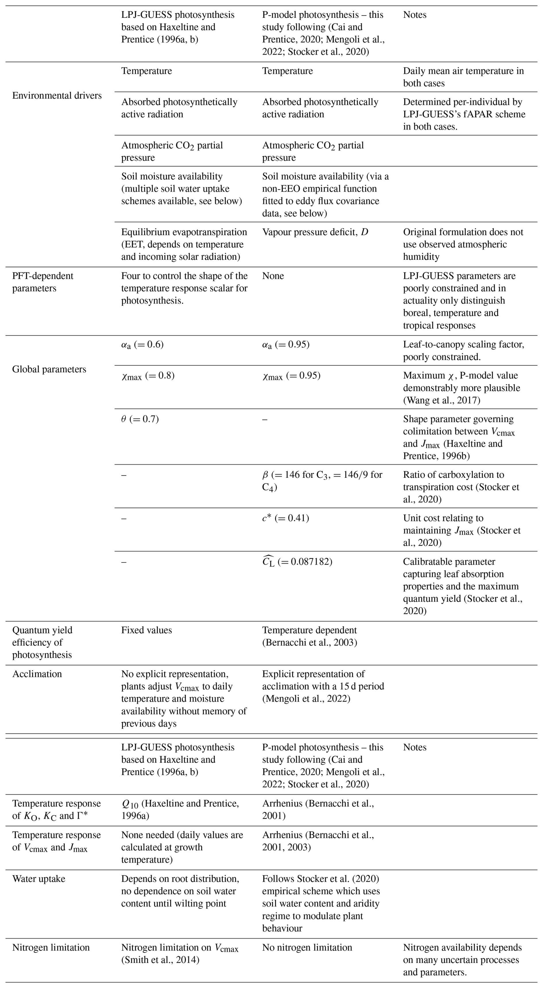
Table 1 Comparison of LPJ-GUESS's original photosynthesis scheme with the P-model implementation of this study.

2.3 Leaf dark respiration

Given that we use mean daily climate inputs in LPJ-GUESS, we cannot implement the acclimation of respiration scheme proposed by Ren et al. (2025) which considers acclimation to both daytime and nighttime temperatures. Instead we use a simpler EEO-scheme which assumes that the dark respiration rate at standard temperature (25 °C), R_d,25, is a constant fraction of V_cmax,25 (Wang et al., 2020). Thus,

$$\begin{array}{}\text{(25)}& R_{\mathrm{d},\mathrm{25}}=b_{\mathrm{25}}\times V_{\mathrm{cmax}\mathrm{25},\mathrm{indiv}}^d\end{array}$$

where b₂₅=0.03 based on fits to experimental data (Wang et al., 2020).

Daily leaf dark respiration rates are calculated from R_d,25 and the daily mean temperature using an empirical relationship from Heskel et al. (2016),

$$\begin{array}{}\text{(26)}& R_{\mathrm{d}}=R_{\mathrm{d},\mathrm{25}}\times e^{\mathrm{0.1012}(T-\mathrm{25})-\mathrm{0.0005}\left(T^{\mathrm{2}}-{\mathrm{25}}^{\mathrm{2}}\right)}.\end{array}$$

2.4 Overview of integration into LPJ-GUESS

All P-model and leaf respiration functions were included via a new source code module. Program control was modified using a switch use the P-model photosynthesis which also automatically uses the EEO leaf dark respiration formulation. To improve runtime efficiency by taking advantage of the parameter-sparse nature of the P-model, the P-model optimality calculation (Eqs. 5 and 6) was only performed once per day for C₃ and once per day for C₄ photosynthesis using the daily mean temperature, atmospheric pressure and VPD of that day. After scaling to a standard temperature of 25 °C, this produced daily optimal values for C₃ and C₄ photosynthesis for V_cmax,25 and J_max,25 on a per unit I_abs basis. These daily optimal values are universal for all PFTs of a given photosynthetic pathway because the P-model has no PFT-specific parameters. However, in LPJ-GUESS, individuals have PFT-specific parameters for structural, phenological, and demographic traits which are unchanged here. This, combined with their position in the canopy, gives each individual its own daily I_abs. So the daily optimal values (per unit I_abs) were then multiplied by the daily I_abs value to give a daily optimal V_cmax,25 and J_max,25 for each tree individual as well as for C₃ and C₄ grasses. These values were then used to calculate the acclimated values per individual following the weighted mean approach of Mengoli et al. (2022). This technical optimisation works without any loss of precision because the first use of I_abs is in Eqs. (13) and (14) where it enters linearly, so optimal V_cmax,25, and J_max,25 can be calculated universally on a per unit I_abs basis.

The interface for the coupling of carbon and water fluxes with the rest of LPJ-GUESS was unchanged except that the standard water uptake mechanism, which is the lower of the demand from photosynthesis and supply from the soil, was replaced such that water uptake is determined by the demand from photosynthesis after adjustment by an empirical soil water stress function from Stocker et al. (2020). This results in water uptake being fully consistent with the photosynthetic requirement without consideration of whether the governing mechanism is supply or demand as in standard LPJ-GUESS. In the rare case that available soil water was above zero but insufficient to satisfy the P-model demand at a given time step, photosynthesis is scaled down proportionally to the fraction of the demand satisfied by the available water. Thus, if the P-model water demand is 1.0 mm but only 0.4 mm are available in the soil, photosynthesis would be reduced to 40 %. The standard water supply functionality in LPJ-GUESS was still used, however, to calculate the daily water stress to determine the phenological state of the raingreen tree PFT and grasses to ensure consistency with phenology calculations in LPJ-GUESS which were otherwise unchanged. We used the SMART water uptake scheme (Lapides et al., 2024) since this is most consistent with the EEO assumption that plants will derive water from the total soil volume rather than having a PFT-specific fixed rooting distribution. The SMART scheme also produces somewhat better results than other water uptake schemes in LPJ-GUESS.

The P-model does not consider nitrogen limitation, so the nitrogen limitation of V_cmax of the standard version (Smith et al., 2014) was not enabled in the EEO configuration. However, the full nitrogen cycle, including soil organic matter dynamics, was enabled in the simulations to confirm that the full model code was functioning correctly after the modifications. With one exception, this nitrogen cycling does not affect the GPP calculation or vegetation functioning. The exception is that nitrogen availability does, in principle, affect the relative allocation of biomass to foliage versus fine roots (Smith et al., 2014). However this was found to be a negligible effect here, when this was disabled in the EEO simulation global GPP changed by only ∼0.1 % (data not shown).

2.5 Simulation setups

We tested two model configurations: the current LPJ-GUESS trunk version (git a3506d14, svn r14188), here referred to “LPJ-GUESS Standard”, and the EEO version with both the new photosynthesis and leaf dark respiration changes, here referred to as “LPJ-GUESS EEO”. Both configurations were run globally (with 30 replicate patches) and at each of the FLUXNET sites (with 100 replicate patches). The FLUXNET run configurations differed from the global setting only in their use of the FLUXNET climate data and, in the case of biomes with clear dominant vegetation types such as the forest and grassland biomes, restricted PFT lists to match the vegetation present at the sites (see Table A1). All simulations followed the standard LPJ-GUESS procedure which comprises a 500 years spin-up period (made from detrending and repeating the first 30 years of the climate dataset) followed by a fully transient period from 1901–2022. For the LPJ-GUESS Standard simulations, the first 100 years was simulated without N limitation to build up N pools, and then the vegetation was killed and allowed to re-establish with N limitation enabled (Smith et al., 2014). Following standard LPJ-GUESS protocol, soil C and N pools were extrapolated to an estimate of their long-term equilibrium using 200 years of modelled fluxes recorded during spin up.

2.6 Model forcing data

2.6.1 Global forcing data

We used the current standard forcing setup for LPJ-GUESS at 0.5° spatial resolution for the global simulations. This includes meteorological forcing (daily mean 2 m temperate, daily total precipitation, daily total downward shortwave solar radiation, daily atmospheric pressure, daily specific humidity, daily mean wind speed) from the CRU-JRA v2.4 climate dataset (University of East Anglia Climatic Research Unit, 2023) from 1901 to 2022. Daily mean relative humidity was calculated from atmospheric pressure, specific humidity and temperature. Vapour pressure deficit (VPD) inputs for the P-model were calculated from relative humidity, temperature and atmospheric pressure. The P-model also requires atmospheric pressure as an input. Here we used atmospheric pressure derived from elevation as opposed to the atmospheric pressure from climate dataset. This is consistent with the approach taken in the P-model development papers. The other standard LPJ-GUESS input datasets used were: CO₂ concentration (Friedlingstein et al., 2023); nitrogen deposition (Lamarque et al., 2013) and population density (Klein Goldewijk et al., 2010, used only for the SIMFIRE fire model).

2.6.2 FLUXNET forcing data

We started with all 212 sites available in the FLUXNET2015 dataset (Pastorello et al., 2020), downloaded from the FLUXNET data portal (https://fluxnet.org/data/download-data/, last access: 9 August 2024). We extracted daily climatic variables for each site, including near-surface air temperature, daily maximum and minimum temperature, wind speed, precipitation, shortwave radiation, atmospheric pressure, and relative humidity. Using the site-specific periods of record, bias correction was applied to the CRU-JRA v2.4 climate dataset for each of the climatic variables with the Python package ibicus (Spuler et al., 2024), following the ISIMIP3BASD (Lange, 2019) bias correction methodology. Sites with less than one year of valid data for any required climate variable were excluded, resulting in a final set of 205 sites. For each retained site, observed FLUXNET meteorological data were merged with the bias-corrected forcing time series over the overlapping period, ensuring that in situ observations were used wherever available.

2.7 Evaluation data

The GOSIF GPP product (Li and Xiao, 2019) was used for global evaluation of spatial patterns, interannual variability and trend. The monthly GOSIF GPP data for 2001-2022 were aggregated from 0.05 to 0.5° using simple averaging. GOSIF GPP has recently been reported to overestimate peak seasonal GPP (Chen et al., 2024) and show decreased accuracy under high temperature, low VPD and drought (Qian et al., 2024). Furthermore, asynchronicity in SIF emission and GPP has been reported (Yang et al., 2022). Since these shortcomings could introduce systematic biases in its seasonal cycle of GPP, we evaluated model skill in reproducing the seasonal cycle with daily eddy flux covariance data from the FLUXNET2015 dataset (Pastorello et al., 2020). We excluded cropland (CRO) and wetland (WET) sites since the EEO configuration does not simulate these land cover types. Open and closed shrublands (OSH and CSH respectively) were included to represent arid sites even though the global LPJ-GUESS configuration does not include shrub PFTs. Partitioning of GPP and ecosystem respiration was done using the nighttime method (Reichstein et al., 2005) and only measurement with quality control value > 0.5 used. We selected sites with at least 2 years of data in which at least 30 % of the days had measurements which exceeded the >0.5 threshold. This left a total of 147 sites (see supplementary material for full list and metadata). We focused on GPP averaged over 5 d with the additional requirement that there were valid measurements on at least four of those days, although we also report daily and monthly values.

To examine the effect of the EEO implementation on biome distributions globally, we used potential natural vegetation (PNV) data from Haxeltine and Prentice (1996b) and a matching biome classification scheme for LPJ-GUESS output (Smith et al., 2014). Whilst newer datasets exist (e.g. Hengl et al., 2018), the Haxeltine and Prentice (1996b) dataset, and the accompanying classification scheme, is widely used in the LPJ-GUESS community and provides a well-understood point of reference.

GPP is linearly dependent on both light use efficiency and absorbed radiation and thus any error in fAPAR will propagate to simulated GPP. We therefore investigated the relationship between the error in simulated GPP versus GOSIF GPP and the error in simulated fAPAR versus observed fAPAR. To quantify fAPAR we selected a dataset based on AVHRR LTDR V5 which has had cross-sensor calibration applied, and has been corrected for orbital drift and cloud cover and harmonized with MODIS (Jeong et al., 2024). For our calculation of the modelled fAPAR error, we used data from 2001 to 2021, temporally aggregated to single annual average values and spatially aggregated from 0.05 to 0.5° using simple averaging.

2.8 Evaluation metrics

For comparing spatial maps of GPP we use the normalised mean error (NME, Kelley et al., 2013):

$$\begin{array}{}\text{(27)}& \mathrm{NME}={\mathrm{\Sigma }}_i|y_i-x_i|/{\mathrm{\Sigma }}_i|x_i-\stackrel{\mathrm{‾}}{x}|\end{array}$$

where y_i is the modelled value in grid cell i, x_i is the observed value and $\stackrel{\mathrm{‾}}{x}$ is the mean of the observed values across all grid cells.

As our simulations had different global total GPP, we used the “normalised mean error – step 2” (NME_2, Kelley et al., 2013) when comparing the interannual variability of global total GPP. This metric removes the influence of the mean values by subtracting the mean values from y_i and x_i (i.e. $x_i\to x_i-\stackrel{\mathrm{‾}}{x}$ and $y_i\to y_i-\stackrel{\mathrm{‾}}{y}$ in Eq. 24). The subscript i now indexes over globally summed averaged values.

When evaluating the seasonal cycle against eddy flux covariance data we used the root mean squared error (RMSE) and coefficient of determination (r²).

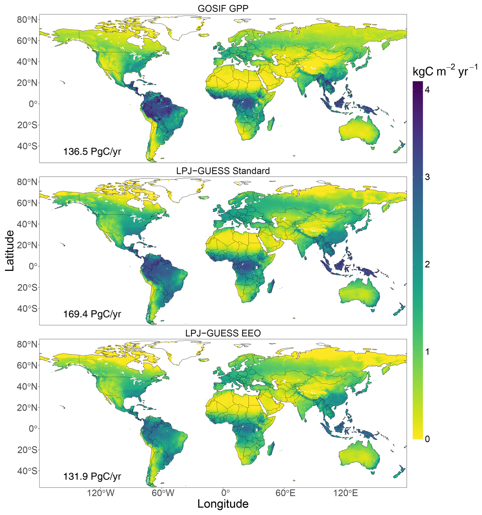
Figure 1 Spatial distribution of mean annual GPP (kg C m⁻² yr⁻¹) for GOSIP GPP and the LPJ-GUESS simulations (mean 2001–2022). The inset numbers are mean annual global GPP.

3 Results

3.1 Spatial and temporal patterns of global GPP

Both model configurations produce spatial patterns of GPP broadly consistent with the observed patterns (Fig. 1). However, the mean annual GPP simulated by LPJ-GUESS EEO is 131.9 Pg C yr⁻¹¹, very similar to the GOSIF GPP estimate of 136.5 Pg C yr⁻¹, whereas the LPJ-GUESS Standard simulation has a larger annual total of 169.5 Pg C yr⁻¹. The LPJ-GUESS Standard overestimated GPP in most regions of the world except in some tropical regions and very high latitudes (Fig. 2). The overall overestimation was much reduced in the LPJ-GUESS EEO simulation, but this configuration underestimates GPP in the tropical forests (Fig. 2). The LPJ-GUESS EEO configuration reduced the NME of the spatial distribution from 0.48 to 0.41 compared to the LPJ-GUESS Standard, an error reduction of 15 %. The simulated GPP vs. GOSIF GPP at the grid cell level (Fig. 3) show reasonable agreement with the one-to-one line, with the LPJ-GUESS Standard showing slightly better fit (goodness-of-fit, r²=0.82; gradient of fitted line, m=0.87) than the LPJ-GUESS EEO simulation (r²=0.79; m=0.72). However, the LPJ-GUESS EEO simulation has an intercept closer to zero (0.25) than the LPJ-GUESS Standard simulation (0.38). These comparisons show that the main improvements produced by the LPJ-GUESS EEO configuration are concentrated in regions with lower GPP (<1 kg C m⁻² yr⁻¹) while the underestimation of GPP by the LPJ-GUESS EEO configuration at high GPP values, corresponding to tropical forests, is responsible for the poorer r² and gradient.

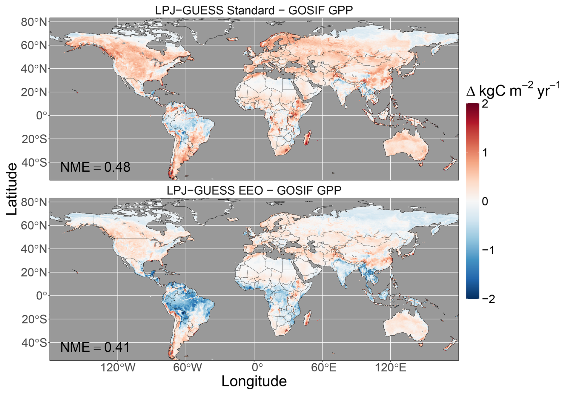
Figure 2 Spatial distribution of difference in mean annual GPP (kg C m⁻² yr⁻¹) for the LPJ-GUESS simulations GOSIF GPP (mean 2001–2022). The inset numbers are the normalised mean errors (NME).

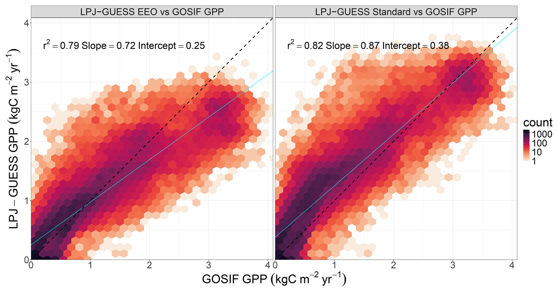
Figure 3 Scatter plot of gridcell-level mean annual (2001–2022) simulated GPP vs. GOSIF GPP (kg C m⁻² yr⁻¹). Black dotted lines are the one-to-one lines, cyan solid lines are fitted lines.

Given the large difference in mean total GPP between the two simulations, we compared the trend and interannual variability in global annual GPP (Fig. 4) after multiplicatively scaling the model simulations to match the first year of the GOSIF GPP data. Both configurations show an increasing trend in GPP over the last two decades, similar though slightly greater than the trend shown by GOSIF GPP. The LPJ-GUESS EEO simulation showed larger interannual variability than either the standard configuration or the GOSIF GPP. However, quantification of model skill using the NME step 2 (NME_2, to account for differences in the mean) shows an error improvement of 32 % in LPJ-GUESS EEO (NME_2 = 0.35) compared to LPJ-GUESS Standard (NME_2 = 0.51).

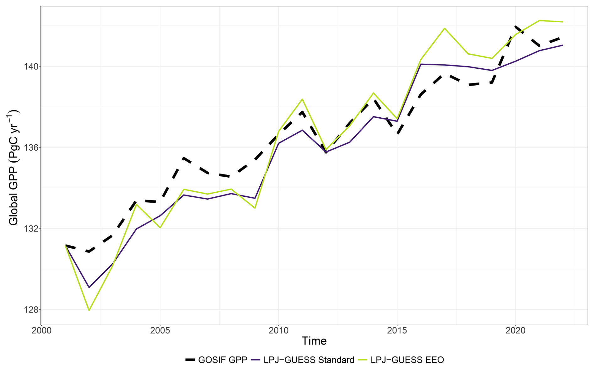
Figure 4 Time series of mean annual GPP (Pg C yr⁻¹) for the GOSIF GPP data and simulations. The simulations have been scaled to match the first year of the GOSIF GPP data.

3.2 Comparison to FLUXNET GPP

There is small but tangible improvement in the simulation of the seasonal cycle with the EEO configuration, (r²=0.48, calculated for 5 d periods at each site and then averaged across all sites) compared to the standard configuration (r²=0.45) at the 147 eddy flux covariance sites (Fig. 5, Table B2). Overall RMSE was the same for the EEO and standard configurations (both 2.7 g C m⁻² d⁻²). The EEO configuration improved the r² fairly evenly across almost all of the IGBP-defined biomes (Fig. 5, Table B2) and improved the shape of the seasonal cycle in the seasonal forest biomes (DBF, MF, ENF) by better capturing the spring increase and the timing of peak GPP better, although underestimating the magnitude of the peak (Fig. 6). The EEO configuration had a poorer r² than the standard configuration for CSH (r²=0.39 compared to 0.54, Table B2), but there are only two sites and the standard configuration does not include a shrub PFT. The performance was also worse for EBF (Table 2), although this is the least well simulated biome in both configurations. Model performance was generally poorer in grassland, shrubland, and savanna biomes than in the seasonal forests, but the EEO configuration generally outperformed the standard model (Table B2, Fig. C1).

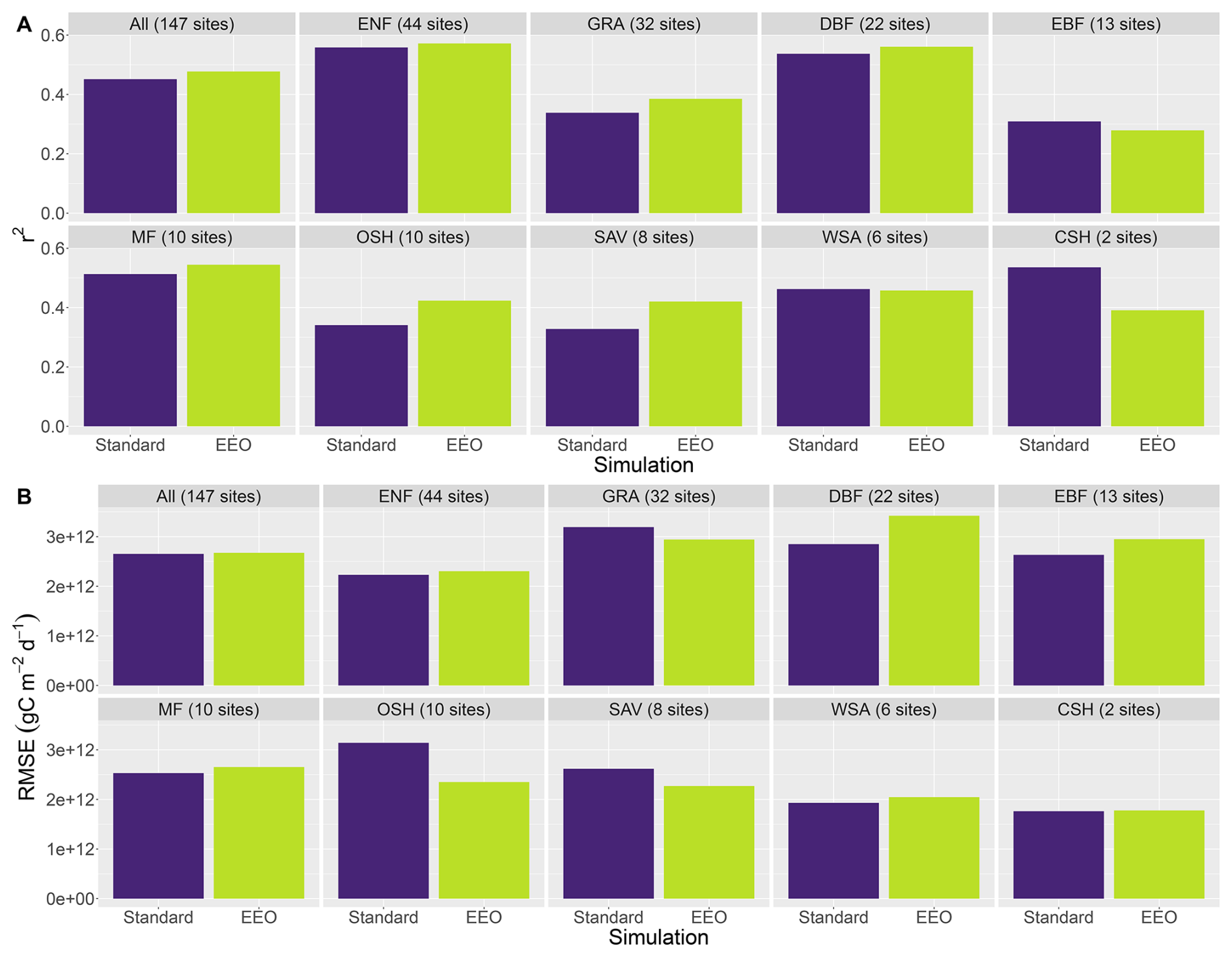
Figure 5 Agreement between site-simulated LPJ-GUESS GPP and FLUXNET2015 averaged across the IGBP classified biomes as quantified by (A) coefficient of determination (r², dimensionless) and (B) root mean squared error (RMSE, g C m⁻¹ d⁻¹).

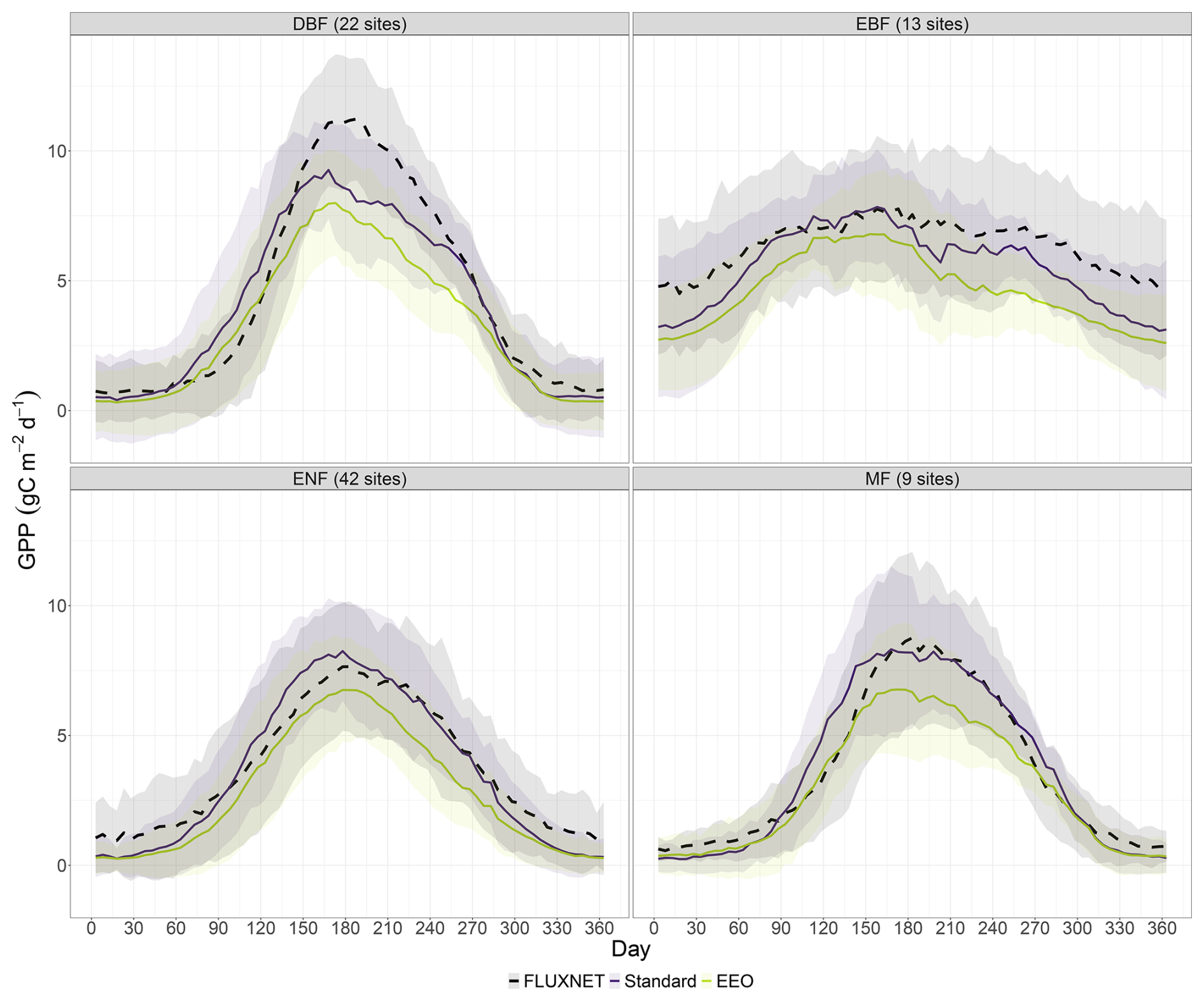
Figure 6 Seasonal cycle of GPP (g C m⁻² d⁻¹) from the LPJ-GUESS site simulations and the FLUXENT2015 data aggregated for deciduous broadleaf forest (DBF), evergreen broadleaved forest (EBF), evergreen needle-leaved forest (ENF) and mixed forests (MF).

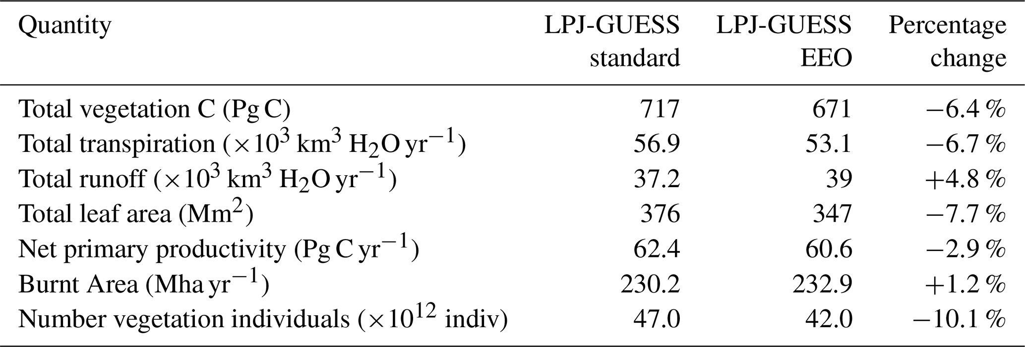
Table 2 Global total values for LPJ-GUESS simulations (mean 2001–2020).

3.3 Leaf dark respiration

The LPJ-GUESS EEO simulation showed significantly lower R_dthan the LPJ-GUESS Standard simulation (Fig. 7). This occurred most obviously in the tropical forest regions where LPJ-GUESS EEO also underestimated GPP (Fig. 2). This underestimation of GPP is likely to be, at least in part, due to an underestimation of V_cmax, which would directly cause the underestimation in R_d observed here. The time series (Fig. 8, scaled to the starting value of the LPJ-GUESS EEO simulation), shows the broad features expected based on the global results of Ren et al. (2024), with R_d increasing in both simulations but less so in the LPJ-GUESS EEO simulation due to the explicit representation of acclimation.

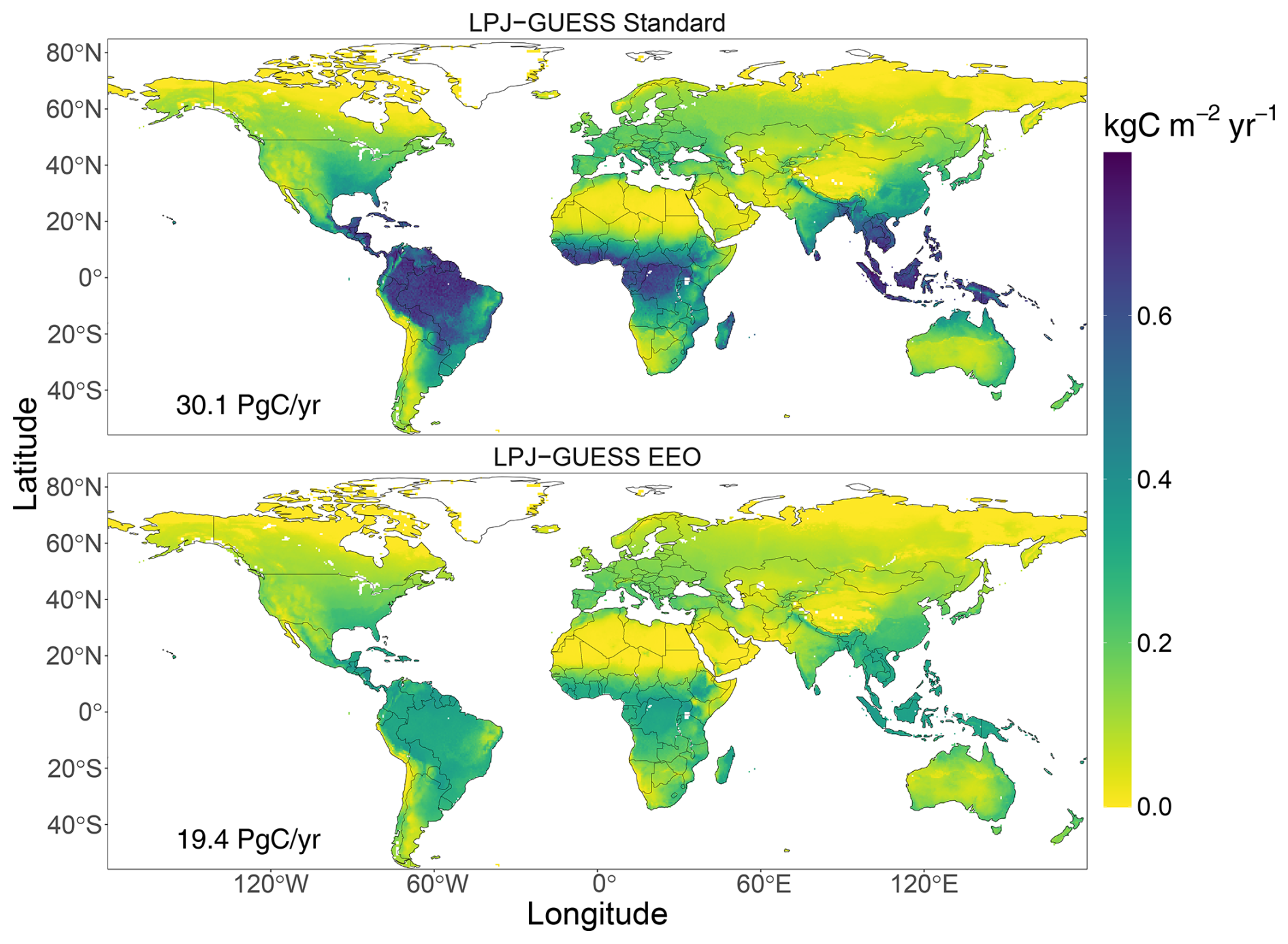
Figure 7 Spatial distribution of mean annual R_d (kg C m⁻² yr⁻¹) for the LPJ-GUESS simulations (mean 2001–2022). The inset numbers are mean annual global R_d.

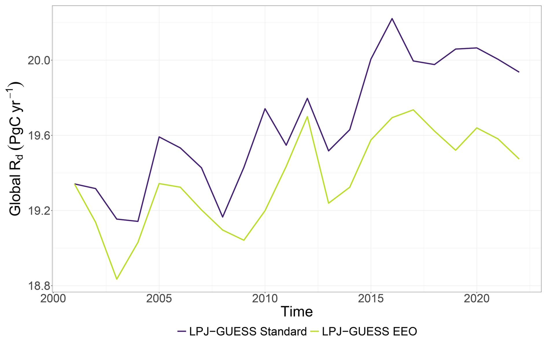
Figure 8 Time series of mean annual R_d (Pg C yr⁻¹) for the LPJ-GUESS simulations. The simulations have been scaled to match the first year of the LPJ-GUESS EEO simulation.

3.4 Impact on global properties

The use of the EEO configuration broadly conserved the simulated global biome distributions (Fig. 9), with only 28 % of the land area changing biome. These changes are concentrated into two distinct zones (Fig. C2). The largest changes occurred at high latitudes, with a large decrease in Arctic/Alpine Tundra which was replaced by Boreal Deciduous Forest/Woodland class (which better matches the PNV biome map) and sharp contraction of Arctic/Alpine Tundra from the highest latitudes (in disagreement with the PNV biomes map). There are also changes in ecotones around arid areas (e.g. the Rocky Mountains, around the Mediterranean Sea, and seasonal tropical areas such as the Cerrado and the African savannas), where biomes switched variously between arid shrublands and woodlands, grasslands, and savanna biomes. In the biome classification scheme these biomes are distinguished by thresholds of woody and grassy LAI (leaf area index) and the ratio between them, so changes of this nature imply shifts in tree and grass competitiveness in water-limited ecosystems. However these changes were not large enough to produce a shift from non-forest to forest biomes (Fig. 9).

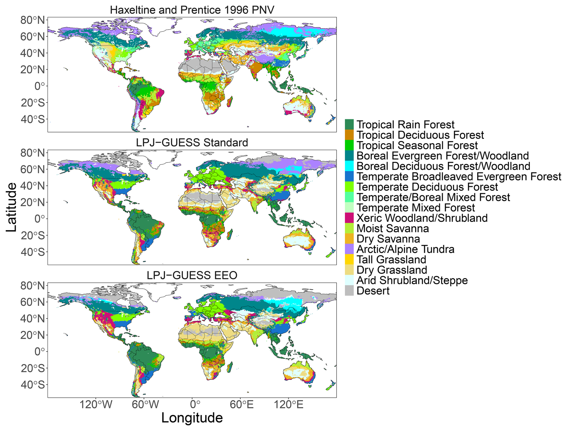
Figure 9 Biome distributions simulated by both LPJ-GUESS configurations based on average LAI between 1961 and 1990 using the classification scheme from Smith et al. (2014) compared to a biome map from Haxeltine and Prentice (1996b).

Global total vegetation C, NPP, LAI, transpiration, and run-off were minimally affected by the EEO changes (Table 2). The broad picture was a little less vegetation biomass, accompanied by a reduction in transpiration and an expected, counter-balancing rise in run-off. Net primary productivity was slightly reduced by −2.9 %. The total number of tree vegetation individuals (a specific property of the LPJ-GUESS model state without a direct real-world analogue) showed a reduction of 10.1 %, a little more than the biomass reduction and so indicated a small effect on tree demographics. Simulated burnt area was not significantly impacted as demonstrated by a small change of +1.2 %.

3.5 GPP error with respect to fAPAR error

Errors in the fAPAR simulated by LPJ-GUESS will directly lead to errors in simulated GPP since we assume that GPP is linearly proportional to fAPAR. Comparison of the error in simulated GPP versus the error in simulated fAPAR on a per-biome basis showed two distinctive patterns, one in the tropical forest biomes (Tropical Rain Forest, Tropical Seasonal Forest and Tropical Deciduous Forest) and one for all other biomes (Fig. 10). In non-tropical forest biomes, the errors in GPP and fAPAR are highly correlated. The correlation of errors in the LPJ-GUESS EEO configuration (Pearson's r=0.72) is stronger than in LPJ-GUESS Standard configuration (r=0.53), but both lines of best fit pass very close the origin and most points lying in the lower-left and upper-right quadrants. In the tropical forest biomes, there is a tendency for both simulations to overestimate fAPAR whilst simultaneously underestimating GPP (slightly more marked in the LPJ-GUESS EEO simulation), resulting in steeper regression lines that did not pass close to the origin. The correlation between the errors was slightly better for LPJ-GUESS Standard for the tropical forest biomes compared to the other biomes (r=0.58), but noticeable worse for the LPJ-GUESS EEO simulation (r=0.53).

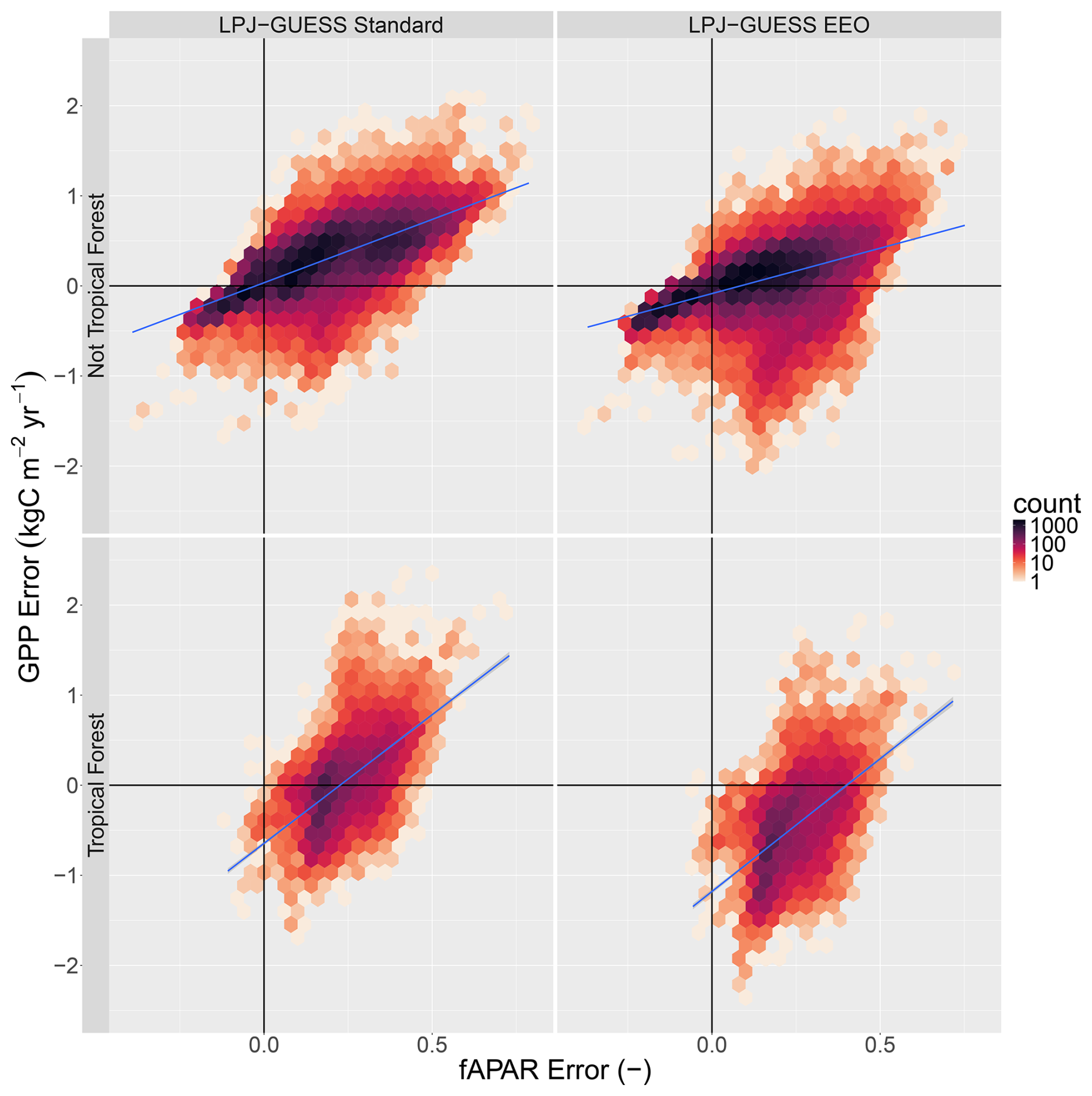
Figure 10 Comparison of error in simulated GPP and error in simulated fAPAR, split into tropical forest biomes and all other biomes (mean 2001–2022). Blue lines are fitted lines.

4 Discussion

The implementation of EEO hypotheses for leaf-level processes, including explicit acclimation, produced realistic results which were in general somewhat better than the original configuration of LPJ-GUESS. This implementation did not degrade the model in other respects.

4.1 Compatibility of EEO formulations with LPJ-GUESS

Overall, we found that including the EEO formulations in LPJ-GUESS produced reasonable results without the need to make major compensating changes elsewhere in the model in terms of process representations or parameter values. This indicates that the EEO formulations did not cause large disruptions in the model functioning and highlights a good degree of compatibility between LPJ-GUESS and the EEO hypotheses. There were changes in biome classification due to simulated changes in tree and grass competition, but these often occurred in areas where shrubs are an important component of the vegetation (shrubs which are not considered in the simulations). This suggests that further improvements to the simulation of arid ecosystems could be made by including a shrub PFT and refining the competition between grass and woody plants.

The EEO formulations improved the representation of the spatiotemporal patterns of GPP at both global scale and at site level, albeit modestly. These improvements come only from adjusting the light use efficiency (and related water uptake) aspect of the GPP calculation whilst the fAPAR component is simulated using LPJ-GUESS's existing allocation, allometry, phenology, and tree population dynamics and disturbance schemes. These schemes exert a major controlling influence on GPP: allocation, allometry, and the balance between tree recruitment and mortality (in particular wildfires) govern the maximum fAPAR and therefore the maximum GPP attained in the growing season. Phenology (determined by both soil moisture and accumulated temperature sums) is key in determining the seasonal development of fAPAR and hence the timing of GPP. Similarly, both LUE and fAPAR depend on available soil moisture from LPJ-GUESS's standard soil hydrology which substantially underestimate soil percolation rates under saturated conditions and therefore underestimate plant-available soil moisture (Lapides et al., 2024). These comparatively coarse and simple global representations obscure the effects of the P-model on GPP, so the fact that there are nevertheless observed improvements demonstrates the capability of the P-model to improve GPP simulation in vegetation models generally and its compatibility with LPJ-GUESS specifically.

This high level of compatibility may be due to the fact that LPJ-GUESS does not use prescribed PFT-specific V_cmax,25 unlike many other vegetation models. Instead LPJ-GUESS performs a daily calculation of V_cmax based on maximising GPP−R_d. This daily calculation could be considered to be a crude form of optimisation and acclimation, albeit with an unrealistically short timescale for acclimation and non-rigourously defined optimality criteria. This representation of light use efficiency in standard LPJ-GUESS was first formulated approximately three decades ago (Haxeltine and Prentice, 1996a, b) in a comparatively data-poor era. The new formulations implemented here are based on better understanding of how plants behave in a universal (i.e. PFT independent) way and more extensive evaluation than possible then, which increases confidence that the model is doing the right thing for the right reasons and thus will produce more robust future projections.

Previous applications and validations of the P-model have predicted mean responses at the ecosystem level, using either eddy flux covariance data with their implicit footprint (Mengoli et al., 2022; Ren et al., 2025) or aggregated across 0.5° gridcells (Cai and Prentice, 2020; Stocker et al., 2020). Here we apply a P-model variant separately to individuals in LPJ-GUESS's cohort-based vegetation state. All individuals experience the same temperature and VPD and there are no PFT specific parameters in the P-model, so the model yields the same optimal V_cmax and J_max on a per I_abs basis on a given day for all individuals of a given photosynthetic pathway. However, individuals experience different I_abs depending on their position in the canopy and their phenology and thus have different acclimated V_cmax and J_max. We have shown that this approach gives reasonable results when aggregated to the ecosystem level, implying that the P-model can be applied separately to different vegetation elements within a simulated structure. This approach also gives rise to a degree of trait/functional diversity within a modelled locality, even within a given PFT. This topic warrants further study, both in terms of a more detailed analysis of how the P-model affects vegetation structure and succession dynamics in LPJ-GUESS, and how the application of the EEO principles to different vegetation elements generates trait diversity which departs from the community means generally predicted by the theory.

Although LPJ-GUESS's “population mode” (which uses a single average individual per PFT instead of the full cohort structure) is now very rarely used and has not been developed for quite some time, we tested it with EEO configuration to give some indication of how the EEO formulations might work with average-individual type models. The global total GPP increased moderately to 143 Pg C yr⁻¹ and the spatial NME remained unchanged at 0.41 (data not shown). This rather good performance indicated that the EEO approach works well with an average individual representation, which is perhaps to be expected as the EEO formulations were mostly developed and tested at the ecosystem, as opposed to individual plant, level.

4.2 Model performance

In terms of global spatial patterns, the use of the P-model strongly reduced overestimation of GPP in extratropical areas. However, it also significantly exacerbated a small pre-existing underestimation in tropical forest areas and at high latitudes. GOSIF GPP is known to have considerable uncertainty particularly under extreme conditions, with a tendency to overestimate GPP under high temperature and/or high VPD conditions (Qian et al., 2024) and peak season GPP (Chen et al., 2024). This may be responsible for some of the apparent model underestimation in the humid tropics, but cannot explain the smaller model overestimation over much of the seasonal tropics and extratropics.

The P-model configuration improved year-to-year interannual variability in GPP, resulting in a 32 % reduction in error (even after accounting for differences in the mean values). The evaluations using eddy flux covariance measurements showed the EEO configuration improved the representation of the seasonal cycle of GPP in almost all biomes, although it underestimated peak summer values in the EBF, DBF, MF and SAV biomes. The P-model predicts a decline in light use efficiency with increasing temperatures (beyond 20 °C) which is not supported by observations (Bloomfield et al., 2023) which may be responsible for this discrepancy. The P-model configuration reduced the positive bias during the spring green up. Nevertheless, there is still a bias; this is a known issue with the P-model (Stocker et al., 2020). The GPP scores were lower those found by Ren et al. (2024) and Mengoli et al. (2022). This is to be expected as the configuration tested here used a fully prognostic framework rather than prescribing fAPAR, leaf area index or soil moisture which introduces additional model error. It also only used daily mean rather than subdaily inputs and so does not resolve the diurnal cycle of photosynthesis.

The high correlation between GPP error and fAPAR error in most biomes (i.e. excluding tropical forests) is revealing as it implies that much of the error in GPP is not due to the error in light use efficiency calculation but rather from the fAPAR calculation. This is particularly encouraging for the P-model as in most biomes it showed notably higher correlation than standard LPJ-GUESS. Dynamics of fAPAR are controlled by LAI in LPJ-GUESS and LAI in turn has two controls; the allometry scheme, which determines the carbon allocated to leaves and therefore seasonal maximum leaf area, and the phenology scheme, which determines how leaf area responds to soil moisture and temperature. Both of these could be targeted to improve LAI and consequently fAPAR and GPP. Recent EEO theory about the controls on LAI (Zhou et al., 2025) may prove informative for both aspects.

The biggest weakness of the EEO setup is the strong underestimation of GPP in tropical forest biomes. We also found the relationship between the errors in GPP and the error in fAPAR to be different in the tropical forests compared to the other biomes. The lines of best fit were steeper and did not pass through the origin, and many of the points were in the “positive fAPAR error, negative GPP error” quadrant, indicating that even if fAPAR was perfectly simulated, GPP would be considerably underestimated, particularly by the EEO configuration. This implies that something different is going on in the tropical forests, particularly when using the P-model. One possible cause of the underestimation is that both the formulation of P-model and the calculation of fAPAR in LPJ-GESS use the Big Leaf approximation (Sellers et al., 1992) which does not account for diffuse radiation. Plants are believed to make more effective use of diffuse radiation, especially in dense canopies through which it can better penetrate (Gu et al., 2003), thus potentially causing the underestimation in tropical forests. Another possible cause is the previously noted decline in light use efficiency at higher temperatures; this will likely strongly impact the tropical forests results. The use of daily climate data may also be a contributing factor.

Another area where the EEO configuration falls short is the very high latitudes where it underestimates GPP and therefore also the extent of the tundra, although the standard configuration shows the same behaviour to a lesser degree. In this case the underestimation can be attributed to the lack of vegetation adapted to extreme conditions (resulting in very short growing seasons) in LPJ-GUESS's standard global PFT set. Other models with more focus on the tundra vegetation, such as BIOME4 (Kaplan et al., 2003), include arctic-focused evergreen shrub types and deciduous PFTs with lower accumulated heat sum requirements (which allows them to respond more rapidly to spring warming and so better take advantage of the short growing season), as does an arctic wetland and methane focussed version of LPJ-GUESS (Miller and Smith, 2012; Wolf et al., 2008).

4.3 Effects of acclimation

There is no indication of a large effect of long-term acclimation to changing climate and [CO₂] on GPP which would cause the two LPJ-GUESS simulations to diverge. This may be because standard LPJ-GUESS does not rely on fixed per-PFT values for V_cmax,25 and already includes a daily optimisation of V_cmax which depends on temperature and [CO₂]. This is a form of acclimation, albeit an unrealistically fast one. However, the inclusion of explicit acclimation may be playing a role in the reduction of the positive bias in the northern hemisphere spring seen in the eddy flux covariance comparisons. The simulations did show a larger effect of acclimation on R_d, as the LPJ-GUESS EEO simulations showed less than half of the increase over 2001–2022 than the LPJ-GUESS Standard simulation in relative terms. In comparison to the global results of Ren et al. (2024) all features are somewhat muted; with lower R_d in the LPJ-GUESS EEO simulation than their equivalent H3 hypothesis results (particularly in the tropics), a smaller increase in overall in R_d, and a smaller difference between the EEO and non-EEO times series. As R_d,25 is linked to V_cmax,25, these differences are likely due, at least in part, to the underestimation of GPP in tropics.

4.4 Other advantages of the EEO configuration in LPJ-GUESS

In addition to improvements in model skill, the EEO configuration provides other scientific and technical benefits. One key advantage is the reduced reliance on poorly-constrained parameter values and process representations. There are four poorly-constrained PFT-specific parameters in the standard LPJ-GUESS which control the shape of the temperature response of photosynthesis. Furthermore, these parameters are fixed, which limits the capacity of photosynthesis to acclimate to changing temperature. These parameters are not used in the P-model configuration. There are also global parameters which are set to more plausible values when using the P-model. The most important is α_a, a canopy-to-leaf scaling parameter that accounts for inefficiencies in plant canopies that cause reductions in PAR utilisation, such as absorption by non-photosynthetic material, leaf clumping, and gaps in the canopy. The standard LPJ-GUESS uses a value of α_a = 0.6, which implies that plants lose 40 % of the potential radiation they could collect due to canopy inefficiencies. The value of 0.95 used in the P-model simulations appears more plausible. The value of 0.95 was an initial guess at a reasonable value and was found to produce reasonable global GPP, but could be further tuned or constrained in future applications. The P-model implementation also sets a maximum value of χ (χ_max) of 0.95, whereas the default LPJ-GUESS value is 0.8. Values of χ>0.8 are not uncommon (Wang et al., 2017), thus the P-model value is more plausible.

The standard LPJ-GUESS has four water uptake schemes but there is no clear rationale for choosing one over the others. The current default choice for global simulations (“ROOTDIST”) calculates water uptake based on soil water and root profile distribution but does not take soil water content into account until plant-available soil water is zero, and so allows the plants to transpire soil water without restriction until it is fully depleted. Two model choices reduce water uptake before plant-available soil water reaches zero, but the parameters have not been derived from observational data. In contrast, the soil moisture stress function used in the P-model configuration was empirically derived from observations (Stocker et al., 2020). Thus, a further benefit of the EEO configuration is to replace an unconstrained model formulation by a formulation that has been calibrated and validated against eddy flux covariance data.

The EEO configuration also has technical advantages. Model runtime was reduced by ∼23% for the global simulations presented here, from 7 h for the standard simulation to 5 h 22 min for the EEO simulation on 384 AMD 7763 CPU cores. This is partly a consequence of the reduced number of vegetation individuals being simulated (∼10 %), which also has the added benefit of reducing the RAM footprint of the model. The remaining runtime reduction was due to the avoidance of the iterative numerical solver routine that standard LPJ-GUESS uses to account for water stress by finding a value of χ that simultaneously balances the transpiration required for photosynthesis and the water uptake possible from the soil. In the LPJ-GUESS EEO configuration the photosynthesis-transpiration calculations take a much smaller share of the runtime.

4.5 Consideration of nutrient limitation

One change introduced by our EEO implementation is that photosynthetic rates are no longer directly affected by nutrient availability as they are in standard LPJ-GUESS, whereby V_cmax is a function of leaf active N (Smith et al., 2014), or by active N and active P in the case of a phosphorus-enabled version (Dantas de Paula et al., 2025). The inclusion of nutrient cycling and the effects of nutrient availability on V_cmax has been considered as a significant achievement of vegetation models, including in LPJ-GUESS (Dantas de Paula et al., 2025; Smith et al., 2014). However, although correlations between V_cmax, as well as J_max, with leaf N and P have been observed in global datasets (Walker et al., 2014), there is little evidence supporting a direct causal relationship that soil N controls V_cmax at the global scale. Recent metanalyses have shown no relationship between soil N and V_cmax,25 at the community level (Peng et al., 2021) and no increase in V_cmax under N fertilisation (Stocker et al., 2025). This is not to say that nutrient availability is not important. The study of Peng et al. (2021) did find a relationship between soil phosphorous and photosynthetic capacity. The study of Stocker et al. (2025) showed that increasing N fertilisation causes increased investment in leaves, and therefore increases GPP via by increasing fAPAR. Furthermore, they presented an optimality-based model (Stocker and Prentice, 2024) which correctly predicts plant responses to both elevated [CO₂] and N fertilisation, which could form the basis for including N limitation on plants in vegetation models on a sounder theoretical footing. However, a simpler and more pragmatic approach for including N limitation in LPJ-GUESS could be to constrain the formation of new leaf biomass based on the N that is available to fulfil the optimal stoichiometry of the new tissue (Smith et al., 2014). This optimal stoichiometry could be determined based on EEO-derived relationships which predict leaf mass per unit area (LMA) purely from climatic growing conditions (Dong et al., 2023; Wang et al., 2023) and leaf N from LMA and V_cmax,25 (Dong et al., 2022). In such a framework the existing LPJ-GUESS formulations for N uptake and other aspects of the N cycle could be maintained. Even though the results here suggest that N limitation of GPP might be less important than previously thought, this topic deserves further attention in the future. In the meantime, removing the direct dependence of V_cmax on available N uncouples photosynthesis from the N cycle, and thus removes the dependence of photosynthesis on many uncertain input datasets, parameters, and processes involved in the N cycle, such as deposition data, soil decomposition, optimal C : N ratios, soil leaching, and translocation. The result is a simpler and more robust model which, as we have seen above, gives better GPP predictions.

4.6 Study limitations and outlook

We have combined the standard daily climate input used in LPJ-GUESS with an explicit 15 d acclimation period. This configuration deviates from the subdaily P-model (Mengoli et al., 2022) in two ways: (1) the model acclimates to daily mean conditions and not noontime conditions, and (2) the model uses a single daily time step to calculate the fast response and actual photosynthetic rates rather than resolving the diurnal cycle. We have not quantified how far these approximations degrade model performance compared to the full subdaily implementation. This could be investigated in a future study. Alternatively, LPJ-GUESS could be adapted to use a subdaily timestep, as has already been done in a version of LPJ-GUESS modified to function as an LSM (Martín Belda et al., 2022) and maybe also be useful in the context of several coupled models involving LPJ-GUESS (Döscher et al., 2022; Forrest et al., 2020; Weiss et al., 2014). Adopting the full subdaily model is comparatively easy with the current implementation if the subdaily data is available, it is only necessary to use noontime climate variables when calculating V_cmax,opt, J_max,opt and ξ_opt and subdaily (e.g. hourly) values for calculating V_cmax,indiv, J_max,indiv and ξ_acclim at the subdaily timestep.

The simulations presented here focus exclusively on potential natural vegetation (PNV) and do not consider croplands, grazed lands or deforested areas. This results in a conceptual mismatch between the global evaluation data (GOSIF GPP data) and the LPJ-GUESS simulations. However, there are no major discrepancies between simulated and observed GPP in highly agricultural areas (for example in the Midwestern United States) or in grazing lands in either simulation, showing that both the standard and EEO versions of LPJ-GUESS captures GPP in anthropogenically modified landscapes reasonably well. The P-model has been successfully applied to simulate wheat yields globally (Qiao et al., 2021, 2023, 2026), so a full integration with LPJ-GUESS's land use functionality (Lindeskog et al., 2013, 2021) is likely a feasible further development. This would open the door to including such simulations into global carbon cycle initiatives such as the Global Carbon Project (Friedlingstein et al., 2023) and model intercomparison projects such as ISIMIP (Frieler et al., 2024).

We did not exclude FLUXNET sites that could potentially be affected by land use history or anthropogenic disturbance. This choice is reasonable given that we did not model these processes or prescribe PFTs abundances, and our intent was to evaluate performance globally, a scale at which implicitly includes a diverse array of land use and disturbance processes which causes deviations from PNV. Nevertheless, a more rigorous selection of test sites could improve the validation procedure.

5 Conclusions

We incorporated the P-model and a complementary representation of leaf dark respiration into the LPJ-GUESS DGVM. We tested this model configuration globally with full integration with the rest of LPJ-GUESS, i.e. with dynamic vegetation, fully prognostic fAPAR and leaf area index, and full coupling with hydrological cycle. Compared to the standard LPJ-GUESS version we saw moderate improvements in GPP patterns (both globally and at eddy flux covariance sites) accompanied by comparatively minimal impacts on the rest of the model functioning, as quantified by comparatively small (<10 %) changes in global carbon and water fluxes and pools, negligible change in global burnt area, and limited changes to the global biome distribution. Whilst we consider these improvements to be valuable in and of themselves (especially given that no tuning or calibration was applied), this approach brings other advantages, including: an embodiment of recent but well-validated theory which includes sensitivity to previously unconsidered drivers, namely VPD and atmospheric pressure; a reduced reliance on poorly-constrained PFT-specific parameters; decreased model run time; and better motivated scheme for plant water uptake. This work demonstrates the potential for EEO-derived theory to improve vegetation models, both as a general proof-of-concept and as specific, concrete first step for incorporating EEO theory into LPJ-GUESS.

Appendix A: Additional equations

To preserve the flow of the main model description some standard formulations were omitted but are included here for completeness.

A1 Michaelis–Menten coefficient

The effective Michaelis–Menten coefficient for Rubisco kinetics, K(T), was calculated as

$$\begin{array}{}\text{(A1)}& K=K_{\mathrm{c}}\cdot \left(\mathrm{1}+{\displaystyle \frac{o}{K_{\mathrm{o}}}}\right)\end{array}$$

where o is the atmospheric partial pressure of oxygen (pa) given by

$$\begin{array}{}\text{(A2)}& o=\left[{\mathrm{O}}_{\mathrm{2}}\right]\times {\mathrm{10}}^{-\mathrm{6}}\cdot p\end{array}$$

and [O₂] is the mole fraction of oxygen taken as 2.09476×10⁵ ppm (parts per million). K_c and K_o are the Michaelis–Menten coefficients for carboxylation and oxygenation given by

$$\begin{array}{}\text{(A3)}& K_x=K_{x,\mathrm{25}}\cdot f_{\mathrm{arrh}}\left(T_{\mathrm{K}},\mathrm{\Delta }{H}_{\mathrm{a}}\right)\end{array}$$

where x can denote either carboxylation ($K_{\mathrm{c},\mathrm{25}}=\mathrm{39.97}$ Pa, ΔH_a=79 430 J mol⁻¹) or oxygenation ($K_{\mathrm{o},\mathrm{25}}=\mathrm{27}\mathrm{480}$ Pa, ΔH_a=36 380 J mol⁻¹) (Stocker et al., 2020).

A2 Photorespiratory compensation point

The photorespiratory compensation point at a given temperature and pressure, ${\mathrm{\Gamma }}^{*}(T,p)$ is calculated by scaling from ${\mathrm{\Gamma }}_{\mathrm{25}}^{*}$, its value at 25 °C and sea-level pressure (Bernacchi et al., 2001):

$$\begin{array}{}\text{(A4)}& {\mathrm{\Gamma }}^{*}(T,p)={\mathrm{\Gamma }}_{\mathrm{25}}^{*}\cdot f_{\mathrm{\Gamma }}\left(T\right)\cdot {\displaystyle \frac{p}{p_{\mathrm{sealevel}}}}\end{array}$$

where ${\mathrm{\Gamma }}_{\mathrm{25}}^{*}=\mathrm{4.332}$ Pa and f_Γ(T) the Arrhenius function with activation energy = 37 830 J mol⁻¹.

A3 Intrinsic quantum yield of photosynthesis

The intrinsic quantum yield of photosynthesis, φ₀, is calculated separately for C₃ (Bernacchi et al., 2003) and C₄ photosynthesis (Cai and Prentice, 2020). $\widehat{C_{\mathrm{L}}}$ is a calibratable parameter encompassing maximum quantum yield and leaf absorption properties, here set to 0.087182 following (Stocker et al., 2020).

$$\begin{array}{}\text{(A5)}& {\displaystyle }& {\displaystyle }{\mathit{\phi }}_{\mathrm{0},{\mathrm{c}}_{\mathrm{3}}}=\widehat{C_{\mathrm{L}}}\cdot \left(\mathrm{0.352}+\mathrm{0.022}\cdot T^{*}-\mathrm{3.4}\times {\mathrm{10}}^{-\mathrm{4}}\cdot T^{\mathrm{2}}\right)\text{(A6)}& {\displaystyle }& {\displaystyle }{\mathit{\phi }}_{\mathrm{0},{\mathrm{c}}_{\mathrm{4}}}=\widehat{C_{\mathrm{L}}}\cdot \left(-\mathrm{0.008}+\mathrm{0.00375}\cdot T^{*}-\mathrm{0.58}\times {\mathrm{10}}^{-\mathrm{4}}\cdot T^{\mathrm{2}}\right)\end{array}$$

A4 Arrhenius function

When scaling variables to and from their values at 25 °C, the normalised Arrhenius function (or its inverse) was used (Bernacchi et al., 2001)

$$\begin{array}{}\text{(A7)}& f_{\mathrm{arrh}}\left(T_{\mathrm{K}},\mathrm{\Delta }{H}_{\mathrm{a}}\right)=e^{\left(\frac{\mathrm{\Delta }{H}_{\mathrm{a}}\cdot \left(T_{\mathrm{K}}-T_{\mathrm{ref}}\right)}{R\cdot T_{\mathrm{K}}\cdot T_{\mathrm{ref}}}\right)}\end{array}$$

where T_K is the temperature in Kelvin, T_ref is the reference temperature (298.15 K = 25 °C) and R is the universal gas constant (8.3145 J mol⁻¹ K⁻¹) and ΔH_a is the activation energy for the particular quantity.

Appendix B: Additional tables

Table B1 IGBP biome types and enabled PFTs used in the LPJ-GUESS simulations of the FLUXNET2015 sites. The full PFT set is: BNE – boreal needle-leaved evergreen tree, BINE – boreal shade-intolerant needle-leaved evergreen tree, BNS – boreal needle-leaved summergreen tree, IBS – boreal/temperate shade intolerant broadleaved summergreen tree, TeBS – temperate broadleaved summergreen tree, TeBE – temperate broadleaved evergreen tree, TrBE – tropical broadleaved evergreen tree, TrIBE – tropical shade-intolerant broadleaved evergreen tree, TrBR – tropical broadleaved raingreen tree, C3G – boreal/temperate C₃ photosynthesising grass, and C4G – tropical C₄ photosynthesising grass.

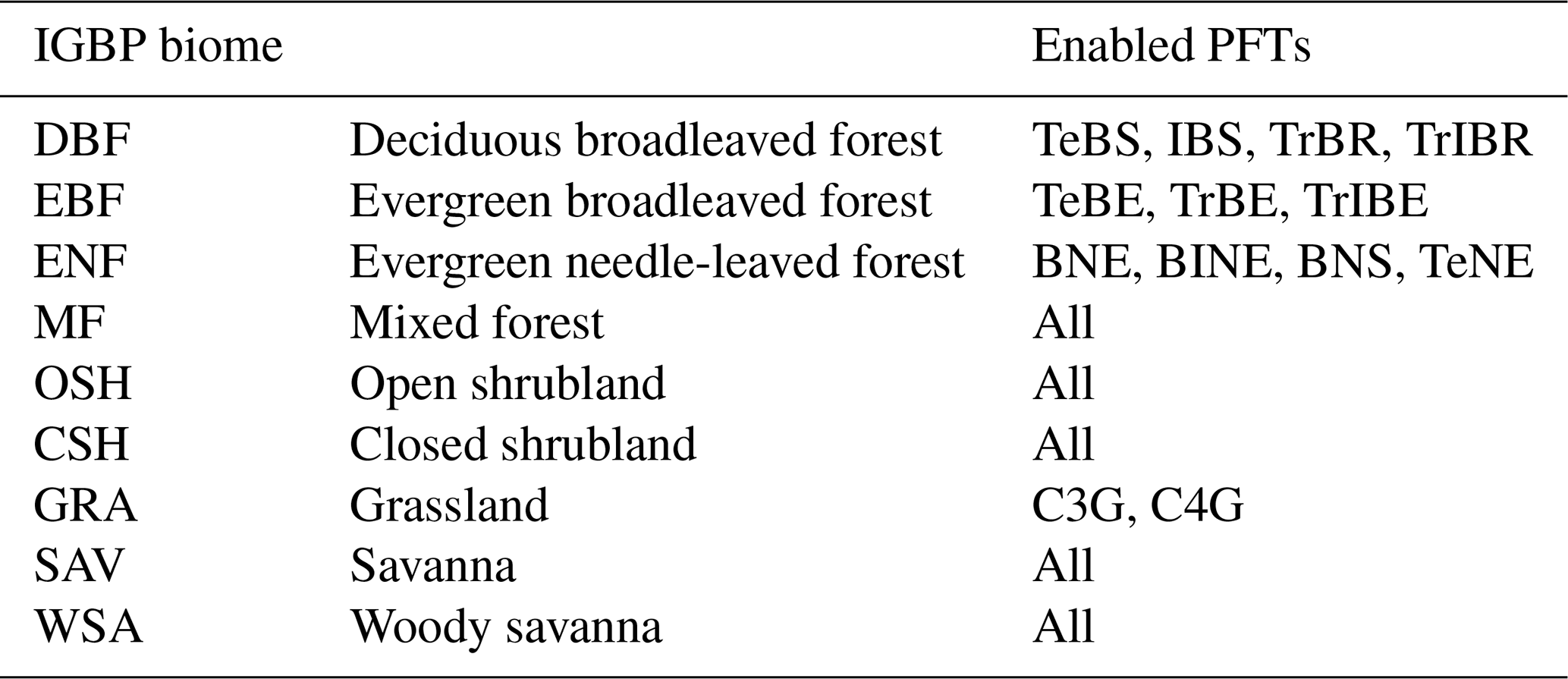
Table B2 Coefficient of determination (r²) and root mean squared error (RMSE) for the LPJ-GUESS simulations compared to FLUXNET2015 sites averaged across all sites and within the IGBP biome categorisation. Bold text indicates better agreement.

Appendix C: Additional figures

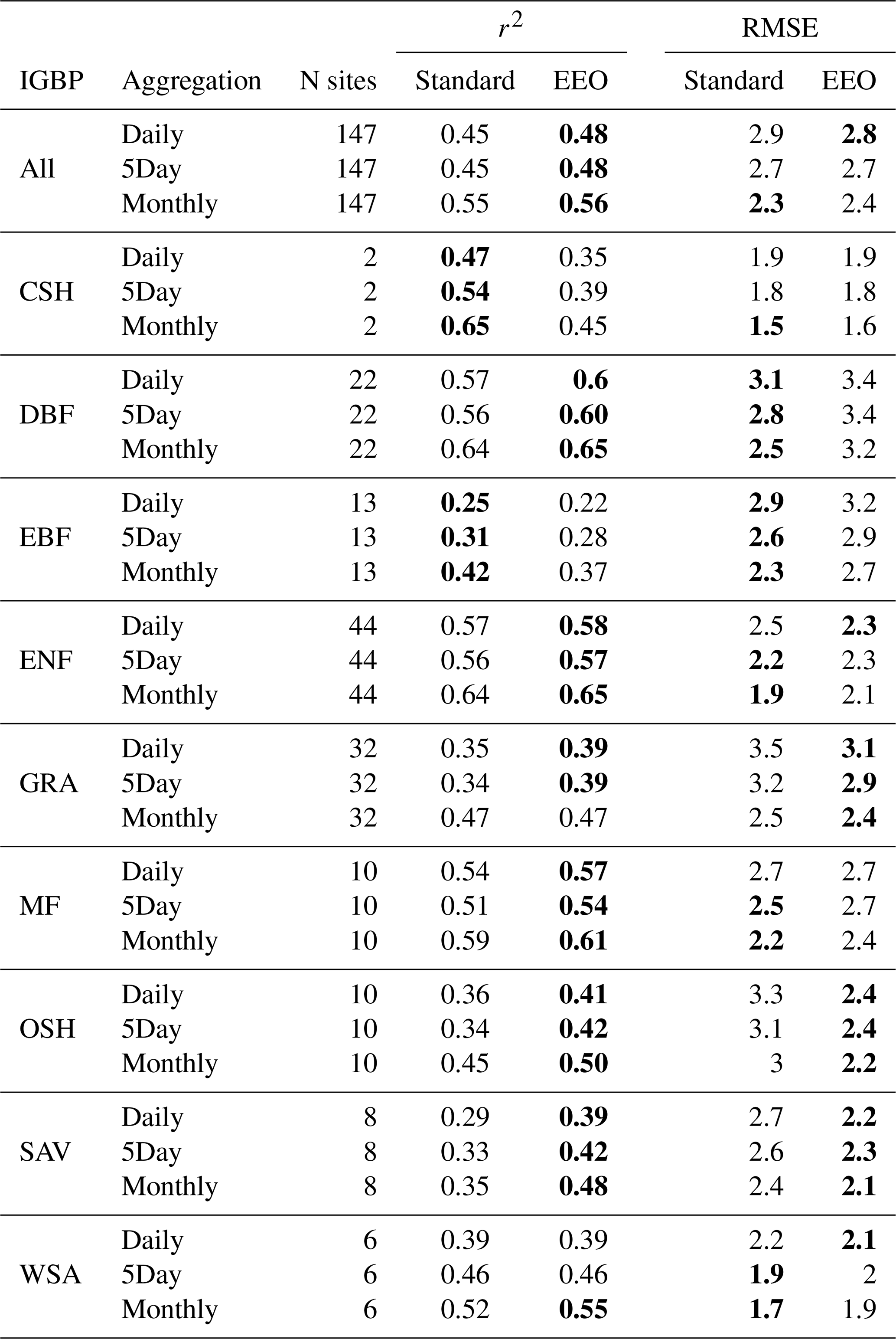
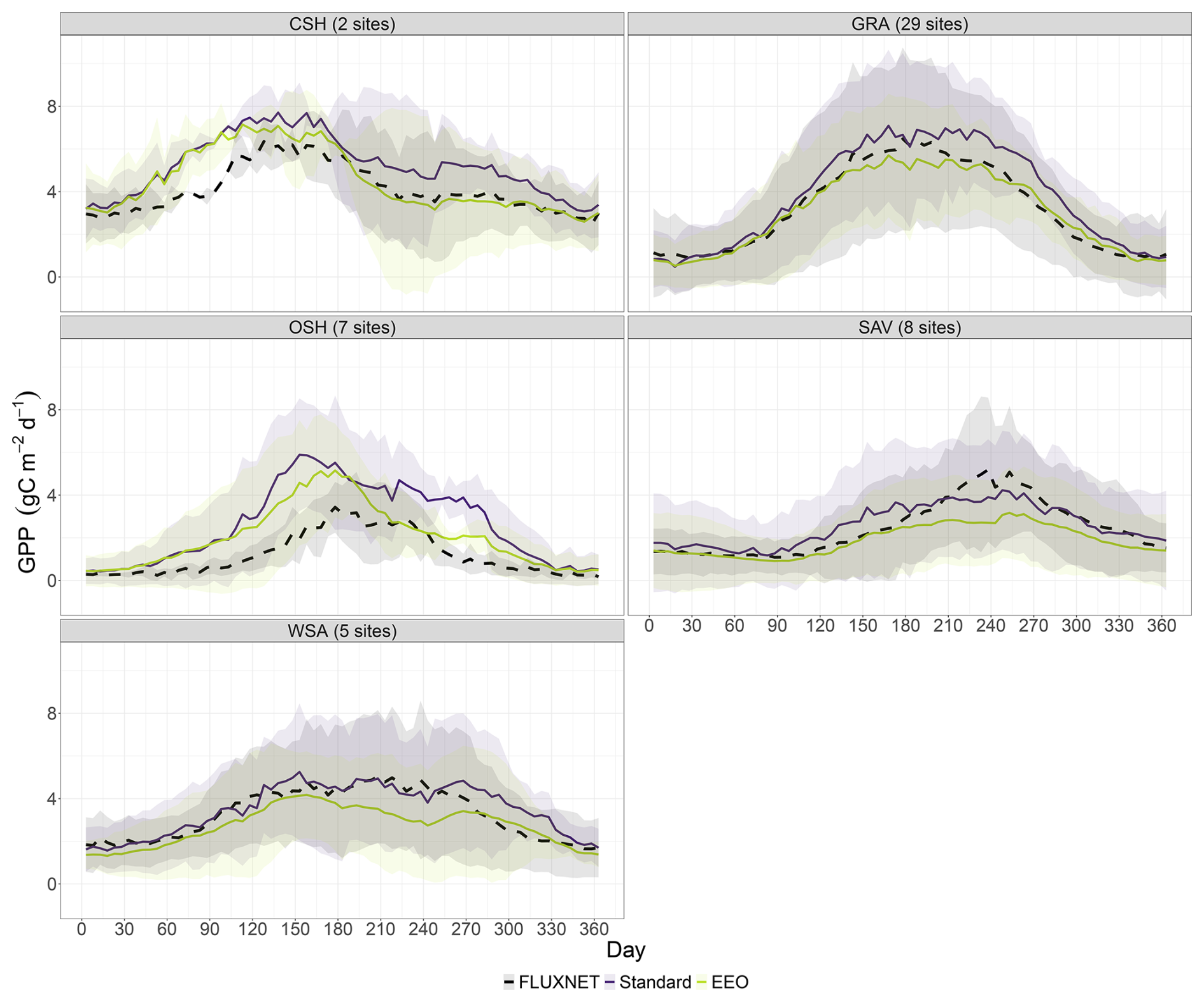
Figure C1 Seasonal cycle of GPP (g C m⁻² d⁻¹) from the LPJ-GUESS site simulations and the FLUXENT2015 data aggregated for closed shrublands (CSH), open shrublands (OSH), woody savannas (WSA), grasslands (GRA), and savannas (SAV).

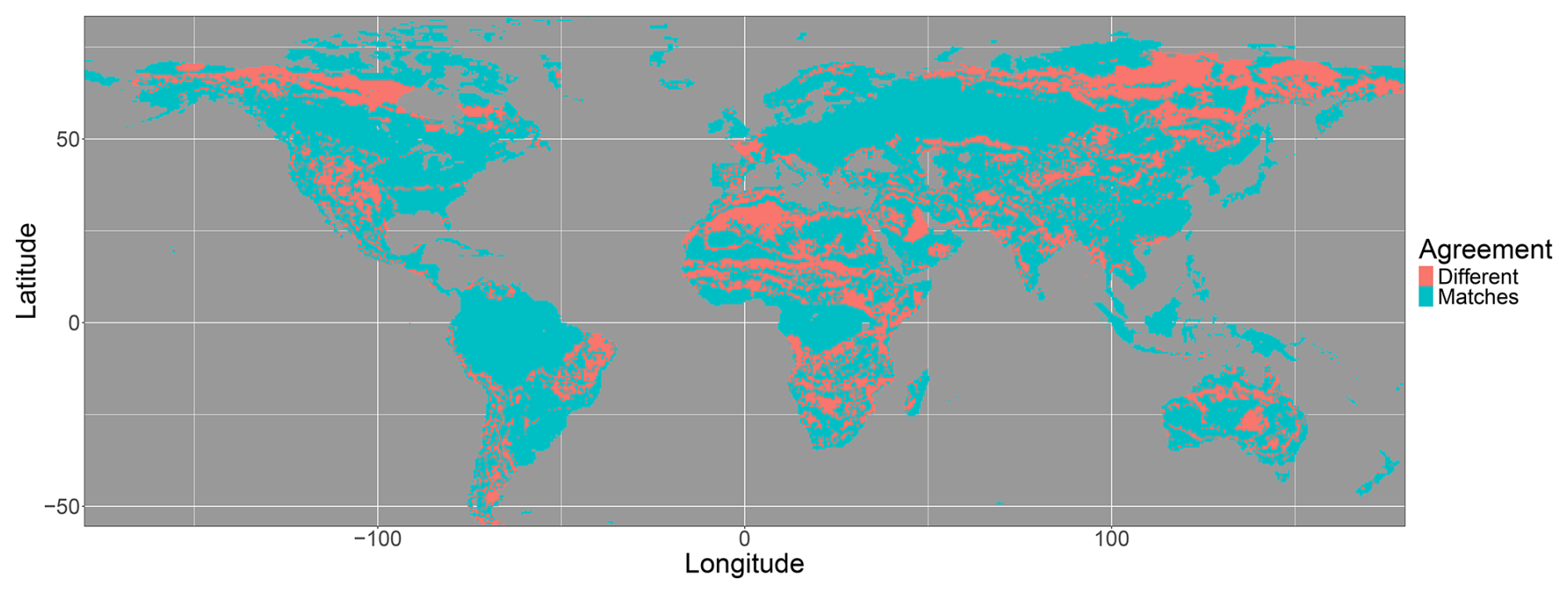
Figure C2 Areas where the biome classifications match or differ between the LPJ-GUESS Standard and LPJ-GUESS EEO simulation. Biomes as derived in Fig. 10.