Using a two-stage Rosenbrock solver to increase computational efficiency in the DOE's Exascale Earth System Model version 1 (E3SMv1)

The integration of stiff atmospheric chemical systems is a major computational cost in Earth System Models and poses challenges for numerical stability as chemical complexity and temporal resolution increase. In this study, we implement a semi-implicit two-stage Rosenbrock method (ROS2) in the Energy Exascale Earth System Model version 1 (E3SMv1) and evaluate it as an alternative chemistry time-integration scheme. ROS2 is tested with two interactive chemical mechanisms of substantially different size: chemUCI (60 prognostic species) and trop_strat_mozart_mam4 (155 prognostic species). Numerical experiments include short simulations to quantify computational cost, a box-model timestep-refinement analysis, and one-year integrations to examine numerical stability and solution sensitivity. At the same 180 s chemistry timestep, ROS2 requires approximately 33 % less chemistry integration time than the original iterative implicit solver on the tested Cori/KNL CPU platform. The magnitude of this speedup is configuration dependent. Global-mean surface-ozone differences among the tested configurations are small (≤ 1.03 ppb), and the one-year integrations show no evidence of numerical instability. Spatial and diurnal differences in ozone, NO, NO₂, and OH are species- and mechanism-dependent, indicating sensitivity to both timestep and solver formulation rather than a common systematic bias. These results support ROS2 as a lower-cost alternative to the current implicit integrator when E3SM chemistry is operated at short timesteps; additional timestep-refinement tests and benchmarking on contemporary CPU/GPU systems are needed to quantify coupled-model convergence and performance portability.

1 Introduction

The development of the Air Quality Model (AQM) has been closely intertwined with the knowledge of photochemical oxidants. The non-linear photochemical ozone formation process, which involves nitrogen oxides, hydrocarbons, and solar radiation, has been recognized as playing a major role in the Los Angeles smog event in the mid-twentieth century (Haagen-Smit, 1952). Reynolds et al. (1973) derived a sequence of mathematical programs to show the dynamical behaviors between chemical emissions and the response of air pollution contaminants. This model numerically represents atmospheric transport, chemical kinetic processes, complex photochemical reactions, and the impact of the emission inventory, and has been used to study urban ozone formation, as well as the precursors of these secondary pollutants. The development of the regional-scale model provides a framework for one-way (from the meteorological process to the chemical reaction) simulations and was eventually extended to a global scale. The chemistry-climate interaction process in the general circulation models (GCMs) has been used to study the global radiation budget, which is affected by tropospheric ozone (Mickley et al., 1999); while the global scale of the chemical transport models (CTMs) has been used to study the tropospheric ozone-NO_x-hydrocarbon chemistry (Bey et al., 2001).

Tropospheric ozone is used as a key diagnostic species in interactive chemistry simulations, yet it is also one of the major air pollutants that has been monitored for decades due to its adverse impacts on human health, ecosystems, and agricultural productivity. Ground-level ozone can trigger respiratory disease, penetrate leaves, and reduce crop yields; therefore, it must be monitored and predicted as both an air pollutant and a climate-relevant species (Markandya et al., 2018; Vandyck et al., 2018). Accurate simulation of surface ozone remains a core capability of numerical models used for air-quality assessment and Earth-system prediction, which also requires consistency of the precursors, for instance the NO_x emission inventory, and other species or photochemical reactions, which leads to an expensive cost in model computation. In the United States, the US EPA has regulated tropospheric ozone under the National Ambient Air Quality Standards (NAAQS) since 1971 (Bachmann, 2007). NAAQS standards have supported monitoring of many chemical species and evaluation of regulatory controls on precursor emissions (e.g., ozone, carbon monoxide, and NO_x). Long-lived species such as ozone have lifetimes spanning weeks to months in the troposphere and will remain relevant through mid-century in future scenarios assessed by the IPCC AR6 (Szopa et al., 2023). In contrast, short-lived species such as NO_x can act as precursors to multiple pollutants (Brasseur et al., 1999), contributing to strong spatial heterogeneity. Because atmospheric chemistry couples species spanning from seconds to months, robust and efficient simulation of such systems remains a major challenge.

To better represent production and loss processes, interactive atmospheric chemistry has increasingly been incorporated into chemistry-climate and Earth system models (Cariolle and Déqué, 1986; Cariolle and Teyssèdre, 2007). Compared with prescribed-chemistry approaches, interactive chemistry allows reaction rates and chemical pathways to respond dynamically to meteorological conditions such as temperature and radiation, improving internal consistency but increasing computational cost. The use of interactive chemistry is still not universal in modern coupled models. Of the 60 coupled climate and Earth system models participating in CMIP6, 32 describe atmospheric chemistry components, while 11 of those use specified or prescribed oxidants in the configurations summarized by IPCC AR6 (IPCC, 2021). Thus, interactive or partially interactive atmospheric chemistry remains present in only a subset of CMIP6 models. This provides a current motivation for numerical methods that reduce the computational burden of solving stiff chemical systems without changing the underlying reaction mechanism.

Although prescribed chemistry can reduce computational cost in global-scale simulations, inconsistent chemistry may compromise internal numerical consistency and lead to biases. For example, ozone production and loss depend on reactive oxygen chemistry, and reaction rates depend strongly on temperature; warming associated with climate change can therefore alter reaction rates relative to those implicit in prescribed concentration fields. This motivates the use of dynamical chemistry solvers that directly couple reaction rates and chemical evolution to the simulated meteorology.

Using a dynamical chemistry solver in an ESM helps maintain numerical consistency between chemical reaction rates and meteorological conditions. Some models, such as WACCM, use simplified gas-phase chemistry (Neale et al., 2012). Other models include interactive chemistry through additional coupled modules, such as LMDZ-INCA (Hauglustaine et al., 2004), in part because of the enormous computational cost associated with solving complex chemical reactions. Yet many GCMs and ESMs aiming to represent more realistic biogeochemical cycles require more complex ozone and tracer chemistry. Examples include linearized ozone chemistry used in stratospheric ozone modeling (Mclinden et al., 2000), the tropospheric model for ozone and related chemical tracers (trop_MOZART) (Emmons et al., 2010), and the more extensive tropospheric-and-stratospheric MOZART (trop_strat_mozart) (Lamarque et al., 2012), which has been used in ESMs such as the Community Atmosphere Model (CAM) within CESM (Neale et al., 2012; Tilmes et al., 2015). However, integrating stiff ODE systems is a major computational bottleneck when simulating species with lifetimes ranging from seconds and minutes to more than one day.

The efficiency of numerical solvers for chemistry interactions is therefore a critical issue (Brasseur et al., 1999; Santillana et al., 2010; Sun et al., 2017). A key difficulty is integrating species spanning a wide range of lifetimes. Models adopt different strategies to address stiffness and timescale separation. For example, the fully coupled model WACCM used an explicit method for long-lived species with weak forcing terms and a fixed 30 min-timestep Newton–Raphson iteration for short-lived species (Neale et al., 2012). Iterative implicit solvers can provide stable integration but may be limited by large timesteps when species lifetimes are minutes or seconds (e.g., during rapid ozone formation). Reducing timesteps can improve fidelity but may increase the number of iterations counts and total computational cost, motivating the development and implementation of more efficient solvers.

Sandu et al. (1997b) compared several implicit solvers, including the Livermore Solver for Ordinary Differential Equations (LSODE), Variable coefficient Ordinary Differential Equation (VODE), Singly Diagonally Implicit Runge–Kutta (SDIRK4), and the Rosenbrock solver RODAS (ROsenbrock-type Differential-Algebraic Solver, a stiffly accurate embedded Rosenbrock method). They concluded that sparse RODAS is more efficient in most test cases. Verwer et al. (1999) further developed a stable second-order two-stage Rosenbrock method (ROS2), suitable for large timesteps on mechanisms such as RIVM (Rijksinstituut voor Volksgezondheid en Milieu, Nathional Institute for the Public Health and the Environment, referred as methane chemistry), CBM-IV (Carbon Bond Mechanism IV), and WET (CBM-IV with liquid-phase chemistry). Sun et al. (2017) implemented ROS2 in the Community Earth System Model (CESM) and found that, at the same timestep, ROS2 reduced the computational cost by 47 % relative to the original numerical scheme.

This paper evaluates ROS2 within the Energy Exascale Earth System Model version 1 (E3SMv1). The atmosphere component, the E3SM Atmosphere Model (EAM), is derived from CAM5 and uses a spectral-element dynamical core that supports global variable-resolution meshes and enhanced vertical resolution (Golaz et al., 2019; Leung et al., 2020). Rosenbrock solvers have previously been evaluated in CESM and in regional atmospheric-chemistry applications, but their implementation and numerical behavior within E3SMv1 have not been systematically assessed. We test ROS2 using two chemistry mechanisms adapted for E3SMv1, chemUCI and trop_strat_mozart_mam4. The mechanisms are not compared as competing chemical representations; instead, they provide numerically distinct testbeds for assessing solver behavior across different system sizes, sparsity patterns, and stiffness characteristics.

We examine three numerical configurations for both chemistry mechanisms. One-day simulations with two CPU core counts are used to quantify relative computational cost. One-year simulations are used to examine numerical stability, temporal behavior, and differences among solver/timestep configurations. The E3SMv1 branches used for the one-year simulations are archived in Tang et al. (2026), and the corresponding model output is archived in Chien and Fu (2026a, b). The purpose of these experiments is to evaluate the numerical integration method within a fully coupled Earth System Model; they are not designed to provide an observational validation of either chemistry mechanism or an absolute accuracy ranking among all tested solver/timestep combinations.

Efficient stiff-chemistry integration remains relevant as Earth system models move toward higher spatial resolution, more comprehensive process coupling, and increased chemical complexity. These developments motivate chemistry solvers that can operate efficiently at shorter timesteps. The present study therefore focuses on solver behavior within the CPU-based E3SMv1 implementation. The timing results reported here should be interpreted as controlled same-platform benchmarks rather than direct evidence of performance on current GPU-accelerated or exascale architectures.

2 Model and Method Used

This study employs the Energy Exascale Earth System Model version 1 (E3SMv1), which was developed to support high-resolution, process-rich Earth system simulations on current and emerging high-performance computing architectures (Golaz et al., 2019). E3SMv1 is designed to address modeling priorities relevant to next-generation CMIP-class simulations, including scalable numerical performance, variable-resolution grids, and enhanced representation of atmospheric processes (Leung et al., 2020). The atmospheric component of E3SMv1, the E3SM Atmosphere Model (EAM), is branched from the Community Atmosphere Model version 5 (CAM5) (Neale et al., 2012) and employs a spectral-element dynamical core. This finite-element formulation enables high-order accuracy, efficient parallel scalability, and regional mesh refinement within a global framework, distinguishing E3SM from many previous chemistry–climate models that rely on finite-difference dynamical cores.

Interactive atmospheric chemistry in EAM is represented here with two mechanisms adapted for E3SMv1. The first, chemUCI, is based on the UC Irvine chemistry-transport formulation (Prather et al., 2017; Tang and Prather, 2012) and contains 60 gas-phase and aerosol species, of which 53 are solved implicitly. It includes 90 chemical reactions and 262 non-zero Jacobian elements after the solver permutation. The second, trop_strat_mozart_mam4, represents more comprehensive tropospheric and stratospheric chemistry and contains 155 gas-phase and aerosol species, of which 130 are solved implicitly. It includes 365 reactions and 1232 non-zero Jacobian elements. The complete permuted species lists are provided in Tables S1 and S2 in the Supplement. These mechanisms are used as numerically distinct testbeds; the objective is not to compare their chemical fidelity or predicted concentrations, but to evaluate ROS2 across different chemical-system sizes and structures.

Atmospheric chemistry is represented mathematically as a system of stiff ordinary differential equations (ODEs) describing reactions with characteristic timescales ranging from seconds to months (Brasseur et al., 1999). In the default E3SMv1 configuration, these equations are integrated using an iterative implicit solver with a fixed chemistry time step, similar to approaches employed in other fully coupled chemistry–climate models such as WACCM. In this study, the second-order Rosenbrock solver (ROS2) is implemented as an alternative chemistry integration method (Verwer et al., 1999). ROS2 is a linearly implicit solver designed for stiff ODE systems and provides second-order temporal accuracy while avoiding costly nonlinear iterations. Previous studies have demonstrated that Rosenbrock-type solvers are efficient and stable for atmospheric chemistry applications (Santillana et al., 2010; Sandu et al., 1997a), and ROS2 has been shown to substantially reduce computational cost when implemented in CESM relative to traditional numerical schemes (Sun et al., 2017).

The ROS2 solver is integrated into the existing E3SMv1 chemistry framework without modification to chemical reaction mechanisms, species definitions, or transport formulations. This design ensures that any differences observed between simulations arise solely from the numerical integration method, rather than from changes in chemical physics or parameterizations. The solver implementation is therefore directly relevant to Earth System Model development, particularly for CMIP7-era simulations that require scalable, numerically robust chemistry solvers capable of supporting higher spatial resolution, increased chemical complexity, and execution on exascale computing architectures.

A series of numerical experiments is conducted to evaluate the performance of the ROS2 solver within E3SMv1. Short-term simulations of one day are performed using different CPU configurations to quantify computational efficiency and chemistry-related computational cost. Longer one-year simulations are used to assess numerical stability, temporal behavior, and the range of simulated chemical concentrations over climate-relevant timescales. Additional sensitivity experiments examine solver behavior under different chemistry time-step configurations. All simulations use identical initial conditions, emissions, boundary conditions, and physical parameterizations to isolate the impact of the chemistry solver.

Solver performance is evaluated using metrics commonly applied in chemistry–climate model development studies, including total wall-clock time, chemistry-related CPU cost, numerical stability, and temporal consistency of key chemical species (Brasseur et al., 1999; Santillana et al., 2010; Sun et al., 2017). These metrics directly address the requirements of scalable and internally consistent chemistry–climate coupling in next-generation Earth system models and support the broader modeling community by enabling more efficient integration of interactive chemistry into CMIP-class and exascale simulations.

The chemical species for each grid in the interactive chemistry mechanism of the E3SMv1 have the equation form, which can be presented as,

$$\begin{array}{}\text{(1)}& {\displaystyle \frac{\mathrm{D}{\mathit{y}}^n}{\mathrm{D}t}}=F\left({\mathit{y}}^n\right)=P\left({\mathit{y}}^n\right)-L\left({\mathit{y}}^n\right)+I\left({\mathit{y}}^n\right)\end{array}$$

where ${\mathit{y}}^n={\left(y_{\mathrm{1}}^n,y_{\mathrm{2}}^n,\mathrm{\dots },y_N^n\right)}^T$ is the vector of volume mixing ratios for N species (N=53 for chemUCI and 130 for trop_strat_mozart_mam4) at time t=tⁿ. The source term F(yⁿ) can be further decomposed into three terms: the production for these chemical species P(yⁿ), the losing term for the consumption of these chemical species L(yⁿ), and I(yⁿ) the independent forcing term, which is based on the external forcing. To solve the set of time-dependent ordinary differential equations, a Jacobian matrix (matrix A in Eq. 2) form of the chemical equations is established. For each element of A_ij is the reaction rate parameterization for reactant i to product j. For the chemical system $\mathrm{D}{\mathit{y}}^n/\mathrm{D}t=F\left({\mathit{y}}^n\right)$, the Jacobian element $J_{ij}=\partial F_i/\partial C_j$ represents the sensitivity of the chemical tendency of species i to the concentration of species j. Because most species do not interact directly through every reaction pathway, the Jacobian is sparse. The fixed species permutation used by the solver changes only the ordering of the unknowns, not the chemistry.

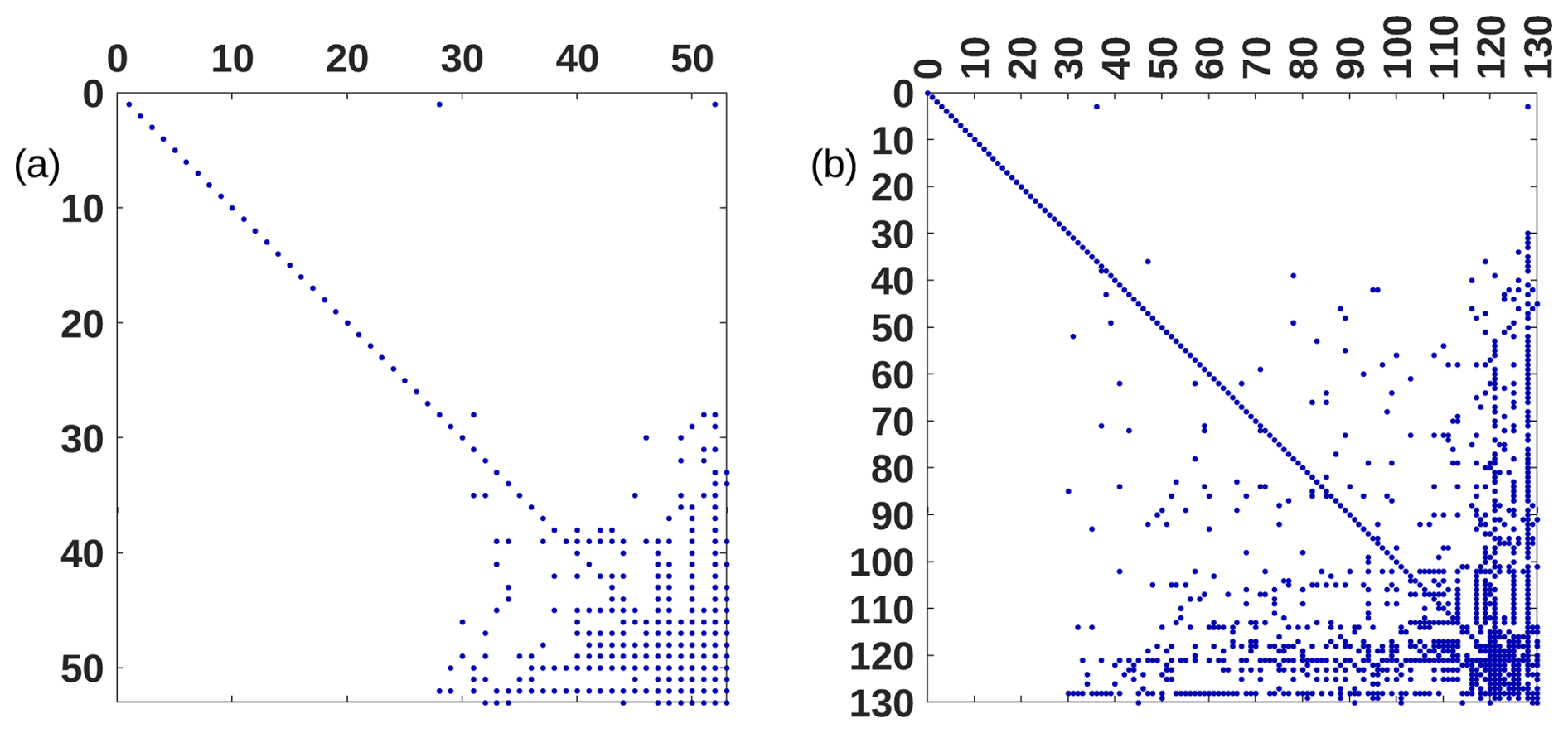
Figure 1 Sparsity pattern of the chemistry Jacobian for (a) chemUCI (53 implicitly solved species) and (b) trop_strat_mozart_mam4 (130 implicitly solved species). For $J_{ij}=\partial f_i/\partial C_j$, the x-axis gives the permuted concentration/state-species index j and the y-axis gives the permuted tendency/equation-species index i. Each blue point denotes a non-zero Jacobian element. The corresponding species order is provided in Tables S1 and S2.

With the specific order of chemical species for each mechanism, non-zero elements occur only at a fixed location (i,j) of the Jacobian matrix. The specific order of the chemical species can be seen in Table S1 (for chemUCI), and Table S2 (for trop_strat_mozart_mam4). The blue dots in Fig. 1a and b show the location of the non-zero elements in the Jacobian matrix. The Newton-Raphson iteration has been adopted as the numerical solver in some global climate models, such as CESM (Neale et al., 2012). This iterative solver benefits from its long timestep and can use the same timestep as the atmospheric component. However, using a long timestep may limit the reaction's performance with shorter-lived chemical species. This limitation would result in the use of parameters for these chemical components. Rosenbrock (1963) proposed generalizing the linearly implicit approach by using multiple stages to achieve higher-order consistency. In this study, we implement a two-stage Rosenbrock scheme. The source code for the two-stage Rosenbrock implementation used in this study is archived in Chien and Fu (2026e). The two-stage Rosenbrock scheme (ROS2) is a well-known numerical scheme for solving stiff Ordinary Differential Equations (stiff ODEs). The solution of the ODE equation (Eq. 1) can be achieved by solving the stagewise equation as,

$$\begin{array}{}\text{(2)}& {\displaystyle }\left(\mathbf{I}-h\mathit{\gamma }\mathbf{A}\right){\mathit{k}}_{\mathrm{1}}=F\left({\mathit{y}}^n\right)\text{(3)}& {\displaystyle }\left(\mathbf{I}-h\mathit{\gamma }\mathbf{A}\right){\mathit{k}}_{\mathrm{2}}=F\left({\mathit{y}}^n+h{\mathit{k}}_{\mathrm{1}}\right)-\mathrm{2}{\mathit{k}}_{\mathrm{1}}\text{(4)}& {\displaystyle }{\mathit{y}}^{n+\mathrm{1}}={\mathit{y}}^n+{\displaystyle \frac{\mathrm{3}}{\mathrm{2}}}h{\mathit{k}}_{\mathrm{1}}+{\displaystyle \frac{\mathrm{1}}{\mathrm{2}}}h{\mathit{k}}_{\mathrm{2}}\end{array}$$

where I is N×N identity matrix, h is the timestep and $\mathbf{A}={\frac{\partial F\left(y\right)}{\partial y}}_{y=y^n}$ is the Jacobian matrix at time t=tⁿ. Equations (2) and (3) are two intermediate formulas, with vectors k₁ and k₂ being the intermediate solutions at each stage. Combined with the previous two stages, Eq. (4) can be used to get yⁿ⁺¹, which is the solution vector at time $t=t^{n+\mathrm{1}}$ from yⁿ, the solution vector at time t=tⁿ. The parameter γ is used in the stability function,

$$\begin{array}{}\text{(5)}& R\left(z\right)={\displaystyle \frac{\mathrm{1}+\left(\mathrm{1}-\mathrm{2}\mathit{\gamma }\right)z+\left(\frac{\mathrm{1}}{\mathrm{2}}-\mathrm{2}\mathit{\gamma }+{\mathit{\gamma }}^{\mathrm{2}}\right)z^{\mathrm{2}}}{{\left(\mathrm{1}-\mathit{\gamma }z\right)}^{\mathrm{2}}}}\end{array}$$

This stability function R(z) is A-stable if and only if $\mathit{\gamma }\ge \frac{\mathrm{1}}{\mathrm{4}}$. Furthermore, to have L-stable R(∞)=0, which can fulfill the radical chemistry species with a short life span, the parameter should be chosen as $\mathit{\gamma }=\mathrm{1}\pm \frac{\sqrt{\mathrm{2}}}{\mathrm{2}}$ (Verwer et al., 1999). Here, we set $\mathit{\gamma }=\mathrm{1}+\frac{\sqrt{\mathrm{2}}}{\mathrm{2}}$. Previous research has demonstrated that the ROS2 solver can support chemistry timesteps of approximately 10–20 min for complex chemical mechanisms (Sandu et al., 1997b; Verwer et al., 1999). These studies primarily focused on solver performance in idealized or offline chemical modeling frameworks and emphasized timestep stability rather than solver behavior within fully coupled Earth system models. In such coupled systems, additional constraints arise from interactions with transport, vertical diffusion, and physics parameterizations, which can significantly limit the practical timestep. Sun et al. (2017) showed that, when ROS2 was implemented in the Community Earth System Model (CESM), a much shorter chemistry timestep of approximately 3 min was required under operational model configurations. While adopting a shorter timestep can yield more realistic simulations of fast chemical reactions compared to traditional Newton–Raphson iteration schemes, it also increases computational demands, particularly for high-resolution and chemistry-rich simulations.

The present study extends earlier Rosenbrock-solver evaluations by implementing ROS2 in E3SMv1, whose atmospheric component uses a spectral-element dynamical core and supports variable-resolution meshes. The experiments assess timestep-refinement behavior, same-timestep computational cost, and one-year numerical stability within this model framework. Because the performance measurements were obtained on a specific CPU architecture, the results are used to characterize the E3SMv1 implementation rather than to claim scalability on current leadership-class or GPU-accelerated systems.

The experimental design emphasizes solver behavior under production-relevant configurations rather than idealized test cases. A series of one-day simulations is performed for each solver configuration, using two different CPU core counts, to quantify the chemistry-related computational cost and parallel performance. To evaluate numerical consistency and temporal behavior beyond short-term metrics, one-year simulations are conducted to examine global mean concentrations and diurnal cycles of key chemical species. These simulation durations are sufficient to assess solver efficiency and short-to-intermediate numerical stability in stiff atmospheric chemistry systems, while deliberately avoiding analysis of long-term climate variability or observational comparisons, consistent with the methodological scope of Geoscientific Model Development.

All simulations were conducted on the now-decommissioned Cray XC-40 Cori system at the National Energy Research Scientific Computing Center (NERSC) (Doerfler et al., 2018), using Intel Knights Landing (KNL) processors in stand-alone CPU mode. Each KNL node contains 68 cores. A 693-core configuration was used for the baseline timing experiments, and a 1350-core configuration was used to test the relative timing behavior at a higher level of parallelism. The same hardware and model configuration were used for all solver comparisons. These timings therefore provide a controlled benchmark for the CPU-based E3SMv1 implementation and should not be interpreted as a direct measure of performance on contemporary GPU-accelerated or exascale architectures.

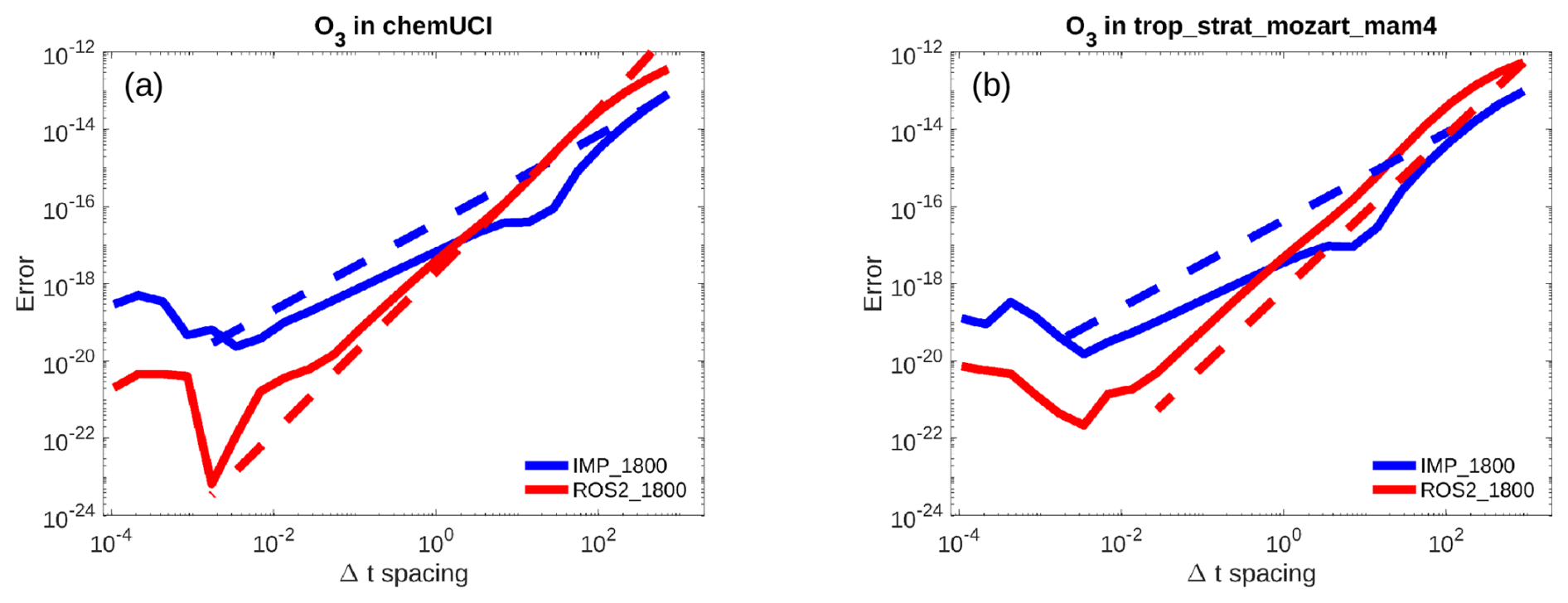
Figure 2 Timestep-refinement error estimate on log-log axes for (a) chemUCI and (b) trop_strat_mozart_mam4. Solid lines show one representative grid column, and dashed lines show the mean fitted trend across 10 000 randomly sampled grid columns. Blue denotes the iterative implicit solver and red denotes ROS2. The fitted slopes are interpreted as empirical convergence-rate diagnostics, not as direct measurements of the formal solver order.

3 Results and Discussion

For a numerically consistent time-integration scheme, the truncation error, ϵ, is expected to scale with a power of the timestep or grid spacing (Ferziger and Perić, 2002; Moin, 2010) and can be expressed as ϵ=o(Δt^k) where k denotes the formal order of accuracy. While such theoretical convergence behavior is well established for idealized systems, its realization in atmospheric chemistry solvers remains uncertain under realistic reaction rates, stiffness, and coupling constraints typical of Earth System Models. Assessing solver accuracy under operational chemical conditions is therefore essential for understanding numerical behavior beyond idealized test problems. To directly evaluate solver accuracy and stability under realistic chemical kinetics, we develop a box-model framework (Chien and Fu, 2026d) that uses actual chemical reaction rates and species interactions extracted from the full Earth System Model (the extracted dataset can be found in Chien and Fu, 2026c). This approach enables controlled numerical testing while retaining the stiffness, sparsity, and multiscale characteristics of operational atmospheric chemistry. The box model is used to evaluate the performance of the original implicit solver (IMP) and the two-stage Rosenbrock solver (ROS2), allowing a direct assessment of numerical behavior without confounding effects from transport or physics parameterizations. The box model is constructed using chemical interaction data from the first simulation day, comprising 49 chemistry timesteps, in both chemUCI and trop_strat_mozart_mam4 configurations. The dataset includes 48 602 atmospheric columns, each with 72 vertical layers, representing a wide range of chemical environments and stiffness regimes encountered in the full model. These data are used to assemble the sparse Jacobian matrix shown in Fig. 1a and b, which faithfully reflects the structure and complexity of the chemistry implicit species numerical solver in a fully coupled Earth System Model. The Jacobian matrix has been permuted to accumulate the non-zero elements in the lower right part of the matrix and hence improved the numerical efficiency in using the LU factorization. By grounding the numerical analysis in real, model-generated chemistry, the box-model framework bridges theoretical numerical analysis and operational Earth system modeling. It provides a robust basis for evaluating solver accuracy, stability, and scalability in a manner directly relevant to next-generation, chemistry-rich, Exascale Earth system simulations. For truncation error ${\mathit{ϵ}}_i=y-y_i$, where y is the analytical solution, and y_i the numerical error. Since we do not know the analytical solution y, when Δt₁ is larger than Δt₂, we can have:

$$\begin{array}{}\text{(6)}& \begin{array}{rl}\left|{\mathit{ϵ}}_{\mathrm{1}}-{\mathit{ϵ}}_{\mathrm{2}}\right|& =\left|y_{\mathrm{1}}-y_{\mathrm{2}}\right|=\left|o\left(\mathrm{\Delta }{t}_{\mathrm{1}}^k\right)-o\left(\mathrm{\Delta }{t}_{\mathrm{2}}^k\right)\right|\\ & \approx \left|o\left(\mathrm{\Delta }{t}_{\mathrm{1}}^k\right)\right|=a\left(\mathrm{\Delta }{t}_{\mathrm{1}}^k\right)\end{array}\end{array}$$

where k is the order of accuracy and ϵ₁ and ϵ₂ are the truncational error based on the timestep Δt₁ and Δt₂. Thus, the error estimation can be expressed as

$$\begin{array}{}\text{(7)}& {\log }_{\mathrm{10}}\left|y_{\mathrm{1}}-y_{\mathrm{2}}\right|={\log }_{\mathrm{10}}a+k\left({\log }_{\mathrm{10}}\mathrm{\Delta }{t}_{\mathrm{1}}\right)\end{array}$$

The log-log slope of the timestep-refinement difference is therefore used here as an empirical convergence-rate diagnostic. Because the analytical solution of the full stiff chemistry system is unavailable and the sampled states are not guaranteed to lie in the asymptotic regime, the fitted slope is not interpreted as a direct measurement of the formal order of either solver.

To quantify timestep-refinement behavior under realistic chemical conditions, the box-model framework uses reaction rates and mixing ratios extracted from the full Earth system model, thereby retaining the stiffness and multiscale character of operational atmospheric chemistry. For both the Newton-Raphson implicit solver and ROS2, the timestep is successively halved beginning at 1800 s. Figure 2 summarizes the resulting error estimate on log-log axes. Results are shown for one representative grid column (solid lines) and for the mean fitted slope across 10 000 randomly sampled grid columns (dashed lines). For chemUCI, the mean empirical slopes are 0.34 for IMP and 0.68 for ROS2; for trop_strat_mozart_mam4, they are 0.30 and 0.50, respectively. ROS2 therefore exhibits a steeper timestep-refinement trend in both mechanisms. These values should not be equated directly with the ideal first- and second-order limits, because the exact solution is unavailable and the full stiff, nonlinear chemical system may not be in the asymptotic convergence regime at all sampled states.

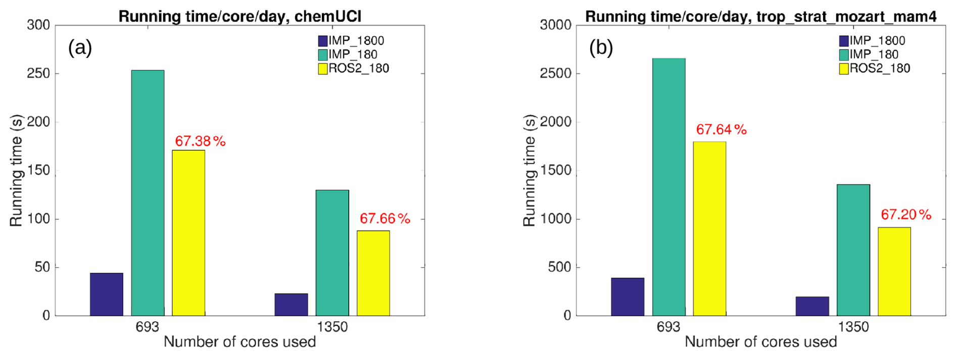
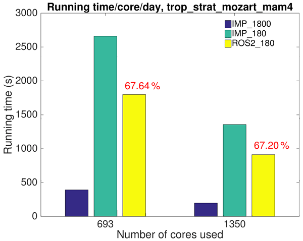
Figure 3 The running time for (a) chemUCI and (b) trop_strat_mozart_mam4. The dark blue is the iterative implicit solver with 1800 s timestep (IMP_1800), and light green is IMP_180, and the yellow is the semi-implicit two-stage Rosenbrock solver with 180 s timestep (ROS2_180) under 693 cores and 1350 cores. The efficiency of ROS2, expressed as a percentage, is shown for each number of cores and chemistry mechanism in red.

To test solver consistency under a perturbed nonlinear chemical regime, the standalone box-model calculations were repeated after reducing external NO_x emissions by 20 %. Figure S1 in the Supplement compares the empirical cumulative distributions of ozone produced by IMP and ROS2 under the baseline (100 % NO_x) and perturbed (80 % NO_x) cases for both mechanisms. The NO_x perturbation changes the chemical state, as expected; however, within each emissions scenario the IMP and ROS2 ozone distributions remain closely aligned. Thus, the solver-to-solver consistency observed under the baseline is retained under the tested NO_x perturbation. This is a targeted numerical sensitivity test; a fully coupled global emissions-perturbation experiment would be required to quantify the complete spatial atmospheric response.

Although the box-model experiments indicate that the timestep of 1800 s is numerically feasible, accumulated numerical errors in a fully coupled climate model may still compromise long-term stability. Consequently, a shorter timestep is required for operational Earth system simulations. Verwer et al. (1999) suggested ROS2 timesteps of 600–1200 s for chemistry models such as RIVM, CBM-IV, and WET. However, due to the finer vertical resolution and stronger coupling constraints in Earth System Models, Sun et al. (2017) recommended a chemistry timestep of 180 s for ROS2 in CESM. Following this guidance, we adopt a 180 s timestep for ROS2 in E3SM, denoted ROS2_180. Two additional numerical configurations are defined for comparison: the original implicit solver with a timestep of 1800 s (IMP_1800, current solver) and the implicit solver with a timestep of 180 s (IMP_180, same solver, with merely the timestep difference). All three configurations use identical reaction rates and matrix mappings, isolating the effects of solver formulation and timestep selection.

The computational cost of each numerical configuration is evaluated using one-day simulations on 693 and 1350 CPU cores (Fig. 3). For trop_strat_mozart_mam4, ROS2_180 requires 67.64 % of the IMP_180 computational time using 693 cores and 67.20 % using 1350 cores. For chemUCI, the corresponding values are 67.38 % and 67.66 %. Thus, at the same 180 s chemistry timestep, ROS2 reduces the measured integration cost by approximately one third relative to the original iterative implicit solver on this platform. The similar percentage reduction for the two mechanisms should not be interpreted as a mechanism-independent scaling law. The relative cost of IMP varies with nonlinear convergence behavior, including additional iterations and timestep subdivision/repetition, whereas ROS2 uses a fixed two-stage update. Consistent with this interpretation, the standalone box-model tests show a broader improvement range of approximately 20 %–48 %. IMP_1800 remains the least expensive of the three tested configurations because it takes one chemistry step for every ten steps at 180 s; therefore, the demonstrated ROS2 performance advantage applies specifically to the same-timestep IMP_180 versus ROS2_180 comparison.

To assess solver behavior over a one-year integration, we compare the spatial distribution of several surface species. Figure 4 shows the surface-ozone difference between ROS2_180 and IMP_1800. For chemUCI, the differences are generally small, with modest positive differences over parts of the Northern Hemisphere and localized regional features. For trop_strat_mozart_mam4, ROS2_180 produces lower surface ozone over much of the globe, with larger negative differences over North Africa. Figures S2–S4 provide corresponding differences for NO, NO₂, and OH. The sign and magnitude of these differences vary by species and mechanism: NO generally shows small decreases, NO₂ changes sign between the mechanisms, and OH differences remain small. No common-sign spatial response is evident across the evaluated gas-phase species. Because these regional patterns can reflect interactions among precursor abundance, radical chemistry, photolysis, transport, and meteorological conditions, the present experiments do not uniquely attribute individual regional differences to emissions or meteorology. A process-budget analysis would be required for that attribution. Aerosol fields are not used as a primary solver diagnostic here because they also depend on aerosol microphysics and phase partitioning, which are not isolated by the present gas-phase time-integration experiment.

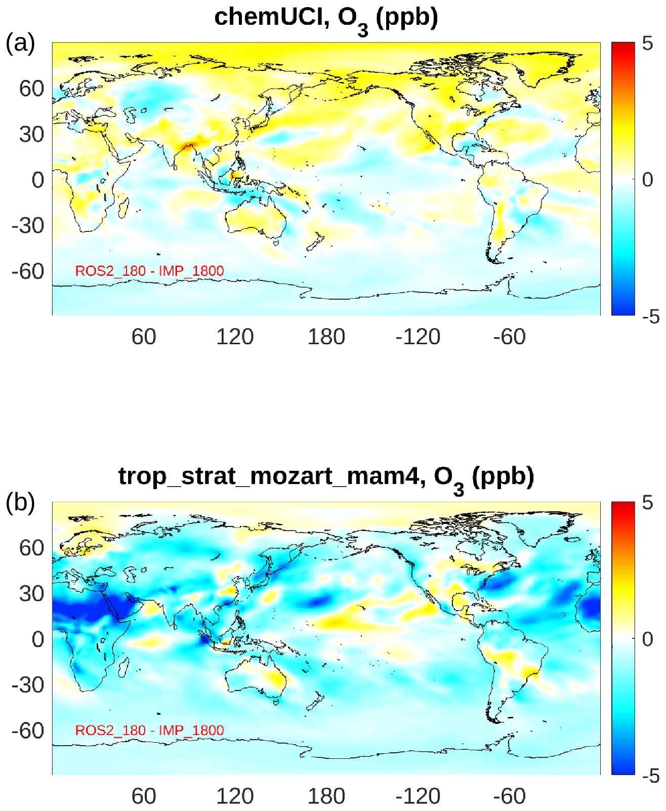
Figure 4 Global surface-ozone difference (ROS2_180 minus IMP_1800) for (a) chemUCI and (b) trop_strat_mozart_mam4.

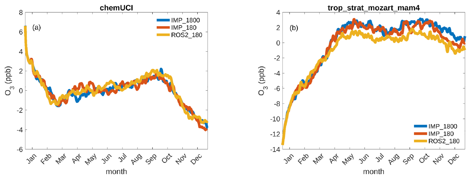
Figure 5 Daily global-mean surface-ozone anomaly (ppb), calculated by subtracting the annual-mean IMP_1800 surface-ozone value from each configuration, for (a) chemUCI and (b) trop_strat_mozart_mam4. Blue denotes IMP_1800, red denotes IMP_180, and dark yellow denotes ROS2_180.

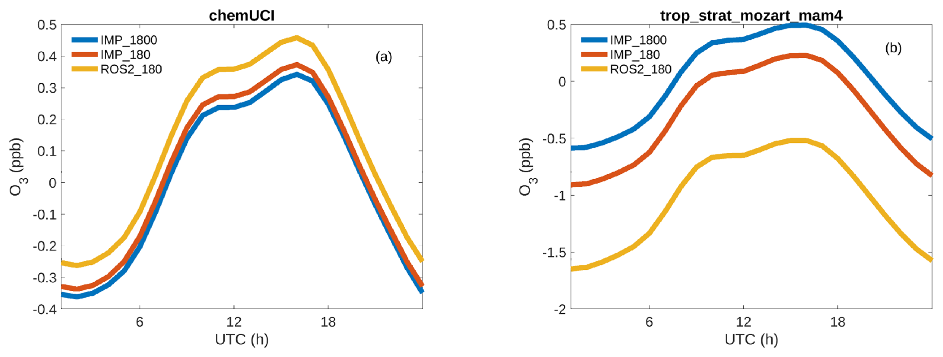
Figure 6 Global surface-ozone diurnal cycle for (a) chemUCI and (b) trop_strat_mozart_mam4. Blue denotes IMP_1800, red denotes IMP_180, and dark yellow denotes ROS2_180. The curves are shown to compare temporal behavior and are not used as an absolute accuracy ranking.

The temporal behavior of surface ozone is summarized in Fig. 5 as a daily global-mean anomaly referenced to the annual mean of IMP_1800. Specifically, the same annual-mean IMP_1800 value is subtracted from all three time series; consequently, the IMP_1800 curve retains its temporal variability about zero and is not expected to remain identically zero. In chemUCI, ROS2_180 follows the annual evolution of the IMP configurations with a mean surface-ozone offset of approximately +0.11 ppb relative to IMP_1800. In trop_strat_mozart_mam4, ROS2_180 also reproduces the broad annual variability but has a mean offset of approximately −1.03 ppb. These differences describe solver/timestep sensitivity and are not used as evidence that one configuration is absolutely more accurate than another.

Figure 6 compares the global diurnal cycles of surface ozone. In chemUCI, ROS2_180 has a slightly higher mean ozone level than IMP_1800, whereas in trop_strat_mozart_mam4 it has a slightly lower mean. The timing and broad day-night structure remain similar, but the curves are not treated as an accuracy benchmark. In particular, the separation between ROS2_180 and the two IMP configurations shows that solver formulation can influence the mean numerical trajectory. Because no exact reference solution is available for the fully coupled one-year integrations, proximity of one curve to another does not establish an accuracy ranking. The computational result is therefore kept separate: ROS2 is less expensive than IMP when both are operated at the same 180 s timestep on the tested platform.

Figure 7 Global surface diurnal cycles of (a) OH, (c) NO, and (e) NO₂ using chemUCI and (b) OH, (d) NO, and (f) NO₂ using trop_strat_mozart_mam4. Blue denotes IMP_1800, red denotes IMP_180, and dark yellow denotes ROS2_180.

Figure 7 extends the comparison to OH, NO, and NO₂. The sensitivity to timestep and solver formulation is species- and mechanism-dependent. For chemUCI OH and for NO in both mechanisms, IMP_180 and ROS2_180 are relatively close, whereas for trop_strat_mozart_mam4 OH and for NO₂ the solver-dependent separation is more apparent. These differences are expected in a stiff coupled chemical system because individual species sample different chemical timescales and nonlinear pathways. None of the three fully coupled configurations is an exact reference solution; therefore, Fig. 7 is used to diagnose numerical sensitivity rather than to rank absolute accuracy. Establishing coupled-model convergence for individual species would require additional timestep-refinement simulations for both solvers.

Taken together, the experiments show that ROS2 provides a clear same-timestep computational advantage over the original iterative implicit solver in the tested CPU-based E3SMv1 configuration and remains numerically stable over one-year integrations. The spatial and temporal comparisons also show that changing the timestep and changing the solver can both alter individual chemical species, with the relative sensitivity depending on the mechanism and species. These results support ROS2 as a practical alternative for E3SM applications that require short chemistry timesteps, while also defining the limits of the present study: the experiments do not establish an absolute accuracy ranking among the three configurations and do not quantify performance portability on contemporary CPU/GPU architectures.

4 Conclusion

Interactive chemistry mechanisms in Earth System Models play an important role in representing the global radiative forcing and evaluating air quality. For instance, tropospheric ozone is both a major air pollutant and a radiative forcing agent in the lower atmosphere, yet its use in global-scale coupled models remains constrained by the high computational cost. Global-scale simulation remains a bottleneck that becomes increasingly acute as models advance toward higher spatial resolutions and exascale computing.

This study implements the two-stage Rosenbrock (ROS2) chemistry integrator in E3SMv1 and evaluates it with two chemically and numerically distinct mechanisms, chemUCI and trop_strat_mozart_mam4. The primary performance result is a same-timestep comparison: at a 180 s chemistry timestep, ROS2 requires approximately one third less integration time than the original iterative implicit solver on the tested Cori/KNL CPU configuration. The magnitude of this reduction is configuration dependent and should not be interpreted as a universal scaling factor. IMP_1800 is the least expensive of the three tested configurations because of its tenfold larger timestep; thus, the benefit of ROS2 demonstrated here is specifically relevant when a short chemistry timestep is required. Across one-year integrations, ROS2_180 remains numerically stable. Global-mean surface-ozone differences relative to IMP_1800 are small, and the spatial differences in ozone, NO, NO₂, and OH are species- and mechanism-dependent rather than showing a common systematic sign. The diurnal comparisons further demonstrate that both timestep and solver formulation can affect individual species. Because the fully coupled simulations do not provide an exact reference solution, these comparisons are not used to rank the absolute accuracy of IMP_1800, IMP_180, and ROS2_180.

The results therefore support ROS2 as a lower-cost alternative to the current implicit integrator when E3SM chemistry is operated at short timesteps. The present Cori-based timing results provide a controlled CPU benchmark, not a performance demonstration for current exascale hardware. Additional timestep-refinement experiments and benchmarking on contemporary CPU/GPU platforms will be needed to quantify coupled-model convergence, architecture-dependent speedup, and performance portability for future higher-resolution E3SM configurations.