HTAP3-OPNS: ozone, PM, nitrogen and sulphur deposition – multi-model experiments to support the revision of the CLRTAP Gothenburg Protocol

HTAP3-OPNS is a multi-model exercise designed to support the revision of the Gothenburg Protocol under the UNECE Convention on Long-Range Transboundary Air Pollution (CLRTAP). Using an ensemble of Chemical Transport Models (CTMs) and Chemistry-Climate Models (CCMs), this study investigates the long-range transport and impacts of ground-level ozone, particulate matter (PM), and nitrogen and sulphur deposition across different global regions. The project aims to assess the contributions of regional versus extra-regional emission sources, evaluate the suitability of current models, and project changes in air pollution under future emission scenarios and climate conditions. A series of perturbation simulations will enable the development of an ensemble emulator to explore and evaluate potential mitigation strategies efficiently. This paper outlines the scientific and policy questions motivating the study, describes the experimental design, including input datasets, model configurations, and required outputs, and discusses methodologies for data handling and analysis. The results will provide crucial insights for policy decisions aiming to improve air quality, protect human health, and protect ecosystems worldwide.

1 Introduction

The 1999 Gothenburg Protocol (GP) of the United Nations Economic Commission for Europe (UNECE) Convention on Long-Range Transboundary Air Pollution (CLRTAP) was the first international, multi-pollutant, multi-effect agreement aimed at reducing the negative effects of acidification, eutrophication, and ground-level ozone in Europe and North America. Under the GP, national emission reduction commitments were agreed for sulphur dioxide, nitrogen oxides, volatile organic compounds (VOCs) and ammonia, based on cost-effectiveness considerations. In 2012, the GP was amended to include particulate matter and black carbon, broadening its scope to include human health impacts and climate change co-benefits. A recent review of the GP (UNECE, 2022) concluded that current air quality legislation in the UNECE region is insufficient to meet CLRTAP's long-term clean air objectives. Furthermore, the review concluded that global reductions in methane emissions would be necessary to achieve these objectives. The Executive Body (EB) of CLRTAP decided in its December 2023 session to launch the process of revising the GP and requested that the convention bodies contributing to the revisions specifically consider how methane in its role as an ozone precursor could be included in a future version of the GP.

The Task Force on Hemispheric Transport of Air Pollution (TF HTAP) was organized under the CLRTAP with the mandate to quantify the long-range (hemispheric to global) influence of distant sources of air pollution (including methane) in the UNECE region. Previous HTAP assessments (HTAP1 (HTAP, 2010) and HTAP2, https://acp.copernicus.org/articles/special_issue390.html, last access: 1 September 2026) have shown that ground-level ozone is significantly influenced by long-range transport at the intercontinental scale and demonstrated the utility of a large ensemble of models for quantifying these effects and their uncertainty. While the primary policy audience of HTAP assessments is CLRTAP and UNECE member states, the work being organised here is also of scientific and policy significance for other world regions. To support the revisions of the GP, TF HTAP is currently organising a new round of multi-model experiments (HTAP3-OPNS) with the goal of quantifying the long-range contribution to ozone, particulate matter (PM), and the deposition of nitrogen (N) and sulfur (S) in different world regions.

In this document we describe the motivating science and policy questions, the design of the several different sets of experiments to be conducted to answer these questions, the input datasets to be used in carrying out these experiments, and the requested output data fields necessary for the analysis of the experiments and the answering of the science-policy questions. The experiments have complementary roles within the overall HTAP3-OPNS framework. Perturbation simulations using Chemical Transport Models and pre-existing emission scenarios will be used to quantify source–receptor relationships and develop an ensemble emulator for exploring mitigation options, while transient Chemistry-Climate Model simulations will investigate the influence of climate change on future air quality under policy-relevant air pollution control scenarios. Simulations of the recent historical period using a state-of-the-art global mosaic emission inventory will support model evaluation and provide connections with concurrent activities addressing total atmospheric deposition and the impacts of wildfires on air quality.

2 Science-policy questions

The design of the HTAP3-OPNS multi-model experiments can be summarised by the following overarching questions.

• What are the contributions of intra-regional and extra-regional sources to air pollution and its impacts in different world regions?

• How suitable are current models for quantifying these contributions?

• Can we explain the inter-model differences?

• How will these contributions change under different realistic future emission scenarios and under potential future climate change?

While these overarching questions have also motivated previous HTAP assessments, there are several new aspects in HTAP3-OPNS.

• A stronger focus on the impacts of ground-level ozone, especially concerning damage to vegetation.

• A stronger focus on the effects of methane on ground-level ozone.

• A stronger focus on the effects of wildfires on long-range air pollution.

• A stronger focus on total atmospheric deposition, in support of the World Meteorological Organization (WMO) MMF-GTAD (Measurement-Model Fusion for Global Total Atmospheric Deposition) exercise. MMF-GTAD is organised by the WMO and aims to provide comprehensive maps of total atmospheric deposition through the fusion of all available deposition measurements with an ensemble of model runs.

• The use of free-running future simulations with atmospheric chemistry-climate models in addition to an ensemble emulator based on source-receptor relationships.

• Calculation of source/receptor relationships for air pollution based on a future emissions scenario rather than historical emissions.

• Comparison of different methods for calculating source-receptor relationships, such as source perturbation, tagging and adjoint techniques.

We also note that HTAP is currently involved in the organisation of two additional multi-model exercises, which are being coordinated with the HTAP3-OPNS exercise:

• MCHgMAP (Dastoor et al., 2025), organised together with the OESG (Open-Ended Science Group) of the Minamata Convention, with a focus on mercury and the first effectiveness evaluation of the Minamata Convention.

• HTAP3-Fires (Whaley et al., 2025), organised in cooperation with International Global Atmospheric Chemistry (IGAC) BBurned, with a focus on the impacts of wildfires on multiple pollutants (ozone, PM, Hg, POPs).

3 Future emission scenarios for the revision of the Gothenburg Protocol

The basis for all assessment of future air quality in HTAP3-OPNS is the Greenhouse Gas–Air Pollution Interactions and Synergies (GAINS) LRTAP future emission scenarios, a set of emission scenarios produced using the GAINS model (Amann et al., 2011) of the International Institute for Applied Systems Analysis (IIASA), which serves as the EMEP Centre for Integrated Assessment Modelling (CIAM) under CLRTAP. Version 2.1 of the GAINS LRTAP scenarios was produced specifically to support the revision of the GP and is available for download (Klimont et al., 2025).

Model assessments in HTAP3-OPNS will use the “CLE” and “MTFR” scenarios from GAINS, as well as a hybrid “HILO” scenario, which are described in more detail below.

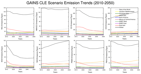
• CLE “Current Legislation”. This scenario is based on economic activity data and an energy mix broadly consistent with SSP2-4.5 (Riahi et al., 2017) and includes all current and planned air pollution control measures and their implementation timelines globally. Emissions of NO_x, NMVOC, CO, CH₄, SO₂, NH₃, PM_2.5, and PM₁₀ from the CLE scenario are shown in Fig. 1.

• MTFR “Maximum Technical Feasible Reduction”. This scenario is based on the same activity data as CLE but includes full implementation of all air pollution reduction measures (including methane reduction measures) which have been shown to be technically feasible (regardless of their cost effectiveness). Economic activity and associated CO₂ emissions are still broadly consistent with SSP2-4.5. Emissions of NO_x, NMVOC, CO, CH₄, SO₂, NH₃, PM_2.5, and PM₁₀ from the MTFR scenario are shown in Figure 2.

• HILO “High methane with low air pollutants”. In addition to the CLE and MTFR scenarios from GAINS, we construct an additional scenario for the purposes of HTAP3-OPNS combining the air pollutant emissions from MTFR and methane emissions from the CLE scenario. This hybrid scenario represents a policy pathway with high ambition on air pollution control, but with minimal ambition on methane control. Economic activity and associated CO₂ emissions are still broadly consistent with SSP2-4.5, as for both CLE and MTFR.

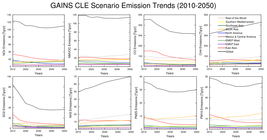
Figure 1 Emissions of NO_x, NMVOC, CO, CH₄, SO₂, NH₃, PM_2.5, and PM₁₀ from the GAINS LRTAP CLE emission scenario.

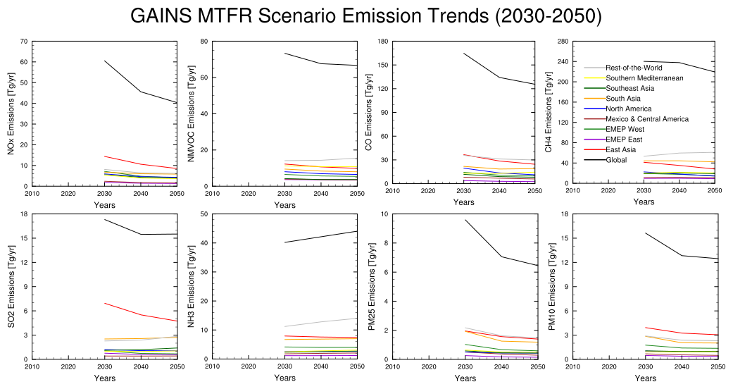
Figure 2 Emissions of NO_x, NMVOC, CO, CH₄, SO₂, NH₃, PM_2.5, and PM₁₀ from the GAINS LRTAP MTFR scenario.

4 Overview of the requested model experiments

The model runs in HTAP3-OPNS are organised into three separate sets of experiments designed to answer the questions outlined above.

• Perturbation experiments with chemical transport models (CTMs) based on the GAINS LRTAP scenarios for the target year 2040.

• Transient Future Scenario experiments with chemistry climate models (CCMs) using the GAINS LRTAP scenarios from 2010 to 2050.

• Transient Historical experiments from 2003 to 2020 using a historical global mosaic emission inventory.

Modelling groups are requested to choose the sets of experiments to which they wish to contribute based on their capabilities, resources, and scientific interests.

4.1 Perturbation experiments for source-receptor relationships and ensemble emulation

As in previous HTAP assessments, we invite groups using global CTMs and CCMs (with specified dynamics from a reference meteorological base year) to perform source perturbation runs for key species/regions/sectors to allow the construction of source-receptor relationships. The year 2015 is chosen as the historical reference year, as this is the year which is currently being considered as the base year for emission reduction commitments under the revised Gothenburg Protocol. At the time, 2015 was the warmest year on record and was characterised by a strong El Niño event (WMO, 2016). Such large-scale modes of climate variability influence atmospheric circulation and can affect the transport and chemical production of ozone, implying that source-receptor relationships and impact metrics will exhibit some degree of interannual variability (e.g., Zhang et al., 2015). Consequently, the source-receptor coefficients presented here should be interpreted as being representative of meteorological conditions in 2015 rather than as invariant quantities.

The use of a single meteorological year represents a compromise between policy relevance, scientific completeness and computational feasibility. The HTAP3-OPNS experiment matrix comprises a large number of perturbation simulations (Sect. 7.1), making it impractical to repeat every experiment for multiple meteorological years across the participating modelling centres. While the magnitude of individual source-receptor coefficients is therefore expected to depend to some extent on the chosen meteorological year, previous HTAP phases and related source-attribution studies have demonstrated that a single meteorological year nevertheless provides valuable information on the relative importance of emission sources and transport pathways (eg. HTAP, 2010).

A key difference with previous HTAP assessments is that the proposed perturbation runs are based on emissions from a future scenario (CLE 2040 from the GAINS LRTAP scenarios) rather than from a historical reference year. The year 2040 is chosen to be consistent with the target year for air quality under the revision of the Gothenburg Protocol. The use of future emissions for the perturbation runs will enable direct construction of source-receptor relationships based on the future distribution of emissions. The key perturbation runs (species/regions/sectors) target the major Northern Hemisphere anthropogenic emission sources, and the model experiments in this set are described in more detail in Sect. 7.1. The development of the ensemble emulator is described in more detail in Sect. 8.2.2.

The source/receptor relationships derived from the perturbation runs will address the question posed in Sect. 2 on the intra- and extra-regional contributions to air quality. The suitability of models for quantifying these contributions will be assessed by both detailed evaluation of models against observations (Sect. 8.2.1) and by the uniformity of the model responses to the perturbations themselves. The diagnostic data requested in Sect. 6 may help to explain inter-model differences. The construction of an ensemble emulator (Sect. 8.2.2) will enable the rapid assessment of alternative future scenarios based on the modelled source/receptor relationships.

In addition to the perturbation runs described in this manuscript, we also invite groups using alternative source attribution techniques such as tagging (e.g. Butler et al., 2020; Mertens et al., 2020) and adjoint sensitivity (e.g. Choi et al., 2019) to perform equivalent runs with their alternative methods and to contribute to the analysis of the different source attribution methods.

4.2 Transient future scenario experiments

In HTAP3-OPNS we invite modelling groups using atmospheric CCMs to contribute transient simulations for the period 2010–2050 using the GAINS LRTAP future anthropogenic emission scenarios and future fire emissions (Sect. 5.2). These simulations serve several purposes:

• Provide a direct assessment of the evolution of air quality under the GAINS LRTAP scenarios.

• Act as a check on the output of the ensemble emulator produced from the Perturbation experiments.

• Allow quantification of the effects of climate change on long-range transport of air pollution.

Climate change is represented in these experiments through the use of forcing datasets (SSTs, long-lived greenhouse gases, etc.) corresponding to the SSP2-4.5 scenario from CMIP6. Under SSP2-4.5, the climate signal by mid-century may remain small relative to interannual variability for some regions and metrics. Quantifying the extent to which the climate-driven response under the GAINS LRTAP scenarios emerges above this variability is therefore one of the objectives of these transient simulations. In 2015 (2050), SSP2-4.5 is associated with atmospheric CO₂ concentrations of approximately 400 (507) ppm (Meinshausen et al., 2020) and CH₄ concentrations of approximately 1834 (2211) ppb (van Caspel et al., 2025). By the 2040–2049 period, SSP2-4.5 is expected to be associated with approximately 0.8 °C additional global warming relative to 2015 (IPCC, 2021).

In order to separate the effects of climate change from the effects of changing emissions on future air quality, we perform an additional set of runs using the GAINS LRTAP scenarios for the period 2010–2050, but with a stationary climate representative of approximately the period 2010–2020, allowing models to generate their own internal meteorological variability. To ensure that the GAINS LRTAP scenarios themselves do not lead to fast responses in modelled climate, this additional set of runs will be performed with composition decoupled from radiation, including the disabling of aerosol-cloud interactions.

The Transient Future experiments are described in more detail in Sect. 7.3.

4.3 Transient historical experiment

We invite groups using CTMs and CCMs to perform specified dynamics simulations from 2003–2020 using the HTAPv3.2 global mosaic inventory (Sect. 5.4) for anthropogenic emissions and biomass burning. These simulations serve several purposes:

• Provide an assessment of the models' ability to simulate observed trends and interannual variability.

• Comprehensive deposition fields from these runs will be provided to the WMO for use in the MMF-GTAD project (https://community.wmo.int/en/activity-areas/gaw/science-for-services/mmf-gtad, last access: 1 September 2025).

• Provide a baseline simulation for additional experiments in the related HTAP3-Fires exercise (Whaley et al., 2025).

The Transient Historical experiment is described in more detail in Sect. 7.4.

4.4 Global to regional downscaling

Regional modelling groups are invited to perform simulations for their region of interest using the GAINS LRTAP emission scenarios and boundary conditions from the global CTMs contributing to HTAP3-OPNS through the Perturbation experiments (Sect. 4.1).

For the European domain, TF HTAP will organise a common set of model experiments designed to support the revision of the GP in cooperation with the CLRTAP Task Force on Measurements and Modelling (TFMM) and the Copernicus Atmosphere Monitoring Service (CAMS). These experiments are described in more detail in Sect. 7.2.

4.5 Additional science questions

Some groups may see an opportunity to piggyback on the HTAP3-OPNS multi-model exercise to answer additional scientific questions (e.g., detailed analysis of ozone budgets, deposition pathways, regionally focused assessments, etc…) and to take a leadership role in the associated analysis. These groups are encouraged to discuss their ideas at TF HTAP meetings and potentially recruit other modelling groups to participate by contributing additional runs or model output parameters.

5 Input data sets

All HTAP3-OPNS model experiments will require modelling groups to use standardised emission datasets for anthropogenic and biomass burning emissions for the defined simulation periods. All other aspects of model configuration, such as natural emissions and meteorological forcing will be left to the discretion of each modelling group, as long as these are consistent with the overall climate forcing required for each model run, which is described for each set of experiments below.

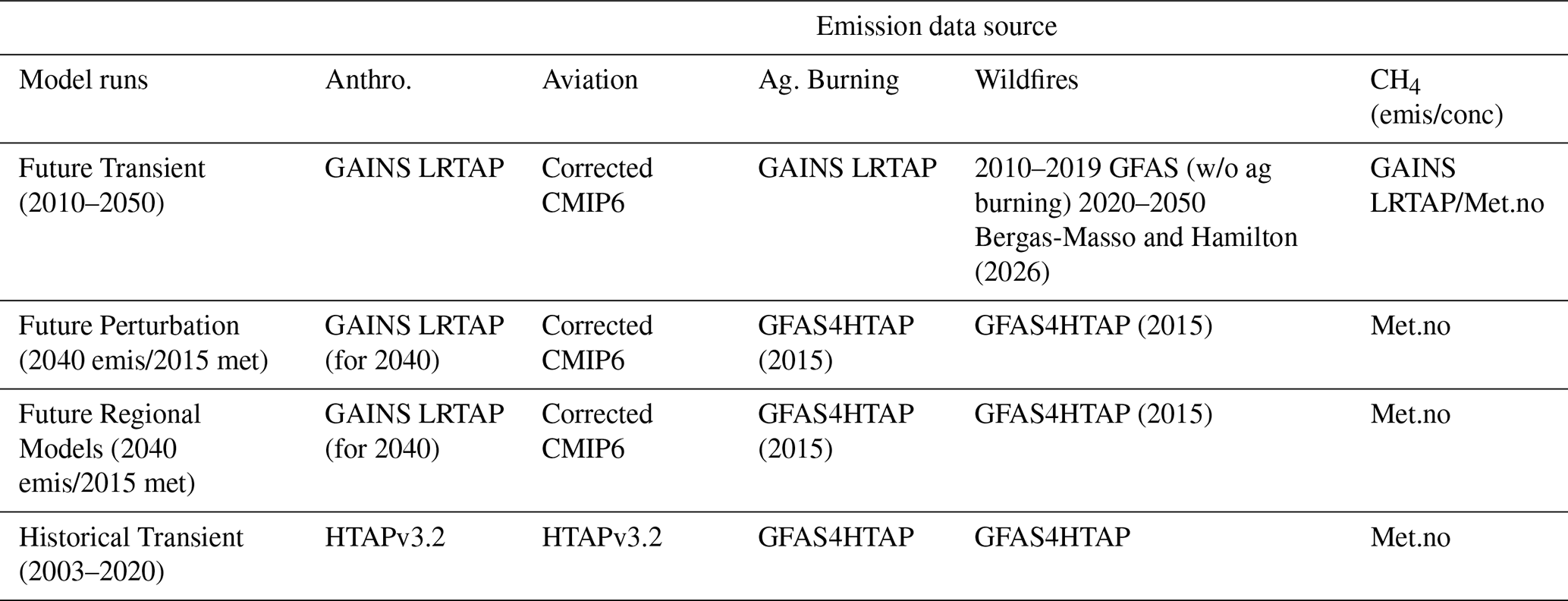
Table 1 shows the emission datasets which should be used for each of the different experiment sets in HTAP3-OPNS. The individual datasets are described in more detail below.

Table 1 Summary of the emission datasets to be used in each of the experiment sets in HTAP3-OPNS. GAINS LRTAP and corrected CMIP6 aviation emissions are described in Sect. 5.1. Future Fire emissions from Bergas-Massó and Hamilton (2026) are described in Sect. 5.2. GFAS4HTAP is described in Sect. 5.3. HTAPv3.2 is described in Sect. 5.4. Methane concentrations from Met.no (Met Norway) are described in Sect. 5.5.

5.1 Anthropogenic future emission scenarios

All model experiments in the Perturbation and Transient Future Scenario sets of experiments must use the GAINS LRTAP version 2.1 anthropogenic emission scenarios. This dataset was introduced in Sect. 3.

The GAINS LRTAP version 2.1 emissions for the CLE and MTFR scenarios are available for download from Klimont et al. (2025) and contain the following emission sectors:

• Energy sector,

• Residential combustion (cooking and heating),

• Transportation,

• Industry (combustion and processes),

• Solvent use,

• Waste management,

• Agriculture (livestock and fertilizer application),

• Open burning of agricultural residues,

• International shipping.

The hybrid HILO (high methane and low air pollutants) scenario is not included in the official GAINS set of scenarios but must rather be constructed by each modelling group by taking methane emissions from the CLE scenario and emissions of all other pollutants from the MTFR scenario. For CTMs and other models using prescribed methane concentrations, methane concentrations are available for all three scenarios (CLE, MTFR, and HILO, see Sect. 5.5).

The GAINS LRTAP scenarios do not provide emissions for the aviation sector. All sets of experiments in HTAP3-OPNS which use GAINS LRTAP scenarios (the Perturbation and Transient Future Scenarios experiments) should use aircraft emissions from the CMIP6 historical and SSP2-4.5 datasets as appropriate for the simulation period. The vertical distribution should be kept as provided in the emission files (with appropriate interpolation to the vertical levels of each participating model to be performed by each group themselves). The correction described in Thor et al. (2023) should be applied to the CMIP6 aircraft emissions. Corrected CMIP6 historical emissions for aviation are available for download from Mertens (2024). Corrected SSP2-4.5 scenario emissions for aviation are available for download from Mertens et al. (2024).

The GAINS LRTAP sector “Open burning of agricultural residues” should be excluded from the Perturbation experiments, which use the historical biomass burning emissions from GFAS4HTAP (Sect. 5.3), as the GFAS4HTAP emissions already include this source. Conversely, the GAINS LRTAP agricultural burning emissions should be included in the Transient Future Scenarios experiments, as the future fire emissions for this set of experiments do not include managed burning. Table 1 provides a summary of the emissions to be used in each set of experiments.

Since the GAINS LRTAP emission datasets include emissions associated with the application of fertilizer, modellers should ensure that their choice of soil NO_x emission inventory does not also include this source.

Modelling groups are free to choose their own chemical speciation profiles, temporal profiles, and injection heights for the GAINS LRTAP scenarios.

5.2 Future fire emissions

All model experiments in the Transient Future Scenario set of experiments (Sect. 4.2) must use the dataset from Bergas-Massó and Hamilton (2026). Future biomass burning emissions from wildfires in this dataset have been prepared based on the output from an ensemble of ESMs with interactive fire models, bias corrected to present-day GFAS4HTAP emissions (Sect. 5.3). These future fire emission datasets correspond to climates simulated in SSP2-4.5 and will also be considered for use in other related multi-model exercises coordinated through HTAP3-Fires, IGAC-BBURNED, and AMAP.

For the model spinup and the period 2010–2020, modelling groups should use biomass burning emissions from GFAS4HTAP (Sect. 5.3). From 2021 onwards, the Bergas-Massó and Hamilton (2026) emissions should be used.

The Bergas-Massó and Hamilton (2026) dataset does not include burning of agricultural waste. As shown in Table 1, all model experiments in the Transient Future Scenario set of experiments should take emissions from agricultural waste burning from the GAINS LRTAP scenarios (Sect. 5.1).

Recommended injection heights for future fires follow Dentener et al. (2006).

5.3 Historical fire emissions

As shown in Table 1, all model experiments performed in the Perturbation and Transient Historical sets of experiments must use all sectors (including agricultural waste burning) from the GFAS4HTAP dataset (Kaiser et al., 2025) which has been developed specifically for HTAP3-OPNS and HTAP3-Fires. To ensure maximum overlap between these related exercises, a common biomass burning emission dataset will be used in both HTAP3-OPNS and HTAP3-Fires. The GFAS4HTAP dataset provides emission fluxes at daily temporal resolution. For HTAP3-OPNS, modelling groups may either use these daily fluxes or aggregate these to monthly mean fluxes.

5.4 Historical anthropogenic emissions

All model experiments in the Transient Historical set of experiments must be based on the monthly mean fluxes for 2000–2020 from HTAPv3.2 (Guizzardi et al., 2025), an update to the HTAPv3 global mosaic emission inventory (Crippa et al., 2023). The HTAPv3.2 dataset is available for download from Zenodo (Crippa, 2025).

Agricultural waste burning emissions from HTAPv3.2 should be excluded from the Transient Historical experiments (Table 1), since these are included in the biomass burning emissions from GFAS4HTAP (Sect. 5.3). Modelling groups are encouraged to use the NMVOC speciation profiles provided with the HTAPv3.2 emission inventory. Modelling groups are free to apply vertical emission profiles to these emissions as they see fit, although HTAP makes no specific recommendation on vertical emission profiles.

Since the HTAPv3.2 emission dataset includes emissions associated with the application of fertilizer, modellers should ensure that their choice of soil NO_x emission inventory does not also include this source.

The Historical Transient experiment is the only experiment in HTAP3-OPNS using the HTAPv3.2 emission inventory (Table 1). For the historical component of the Transient Future and Perturbation sets of experiments, emissions are taken from the GAINS LRTAP scenarios (Sect. 5.1).

5.5 Surface methane emissions and concentrations

For the Transient Future set of experiments, anthropogenic emissions of methane are provided in the GAINS LRTAP future scenarios (Sect. 5.1). Groups with the capacity to perform methane emission-driven simulations should use the GAINS LRTAP anthropogenic methane emission fluxes, along with their own choice of natural methane emissions and any necessary flux adjustment (Folberth et al., 2022).

For all groups performing the Perturbation experiments, and for groups performing the Transient Future experiments without the capacity to perform methane emission-driven simulations, surface concentrations of methane consistent with the GAINS LRTAP emission scenarios CLE and MTFR and the hybrid scenario HILO (high methane and low air pollutants) are provided based on the reduced complexity climate model (RCM) simulations run by MSC-W (Met Norway) driven by emissions from the GAINS LRTAP scenarios. In HTAP3-OPNS, these methane concentrations are named as Met.no. The RCM used for this purpose is the Model for the Assessment of Greenhouse-gas Induced Climate Change v7.5.3, MAGICC7 (Meinshausen et al., 2009, 2011, 2020), following the approach described in van Caspel et al. (2024). In this configuration, the MAGICC7 model is run in its 600-ensemble probabilistic mode (Nicholls et al., 2021) to calculate global mean tropospheric methane concentrations as a function of the anthropogenic emission scenarios. Natural emissions are estimated by closing the methane budget with respect to historical observations up to the year 2023 and are kept constant throughout the simulation period. The MAGICC7 model is calibrated to observations from the NOAA network for the historical period.

Surface methane concentrations for the CLE, MTFR, and HILO scenarios are available for download from Zenodo (van Caspel and Fagerli, 2025). It is important to note that the surface methane concentrations in each of the three scenarios are different. While the HILO scenario uses the same methane emissions as the CLE scenario, the resulting methane concentrations are not identical under CLE and HILO due to the different emissions of NO_x and NMVOC in these scenarios and the consequent effects on ozone, hydroxyl radical, and the methane lifetime. The time series of methane emissions from each of the three scenarios is shown in Fig. 3.

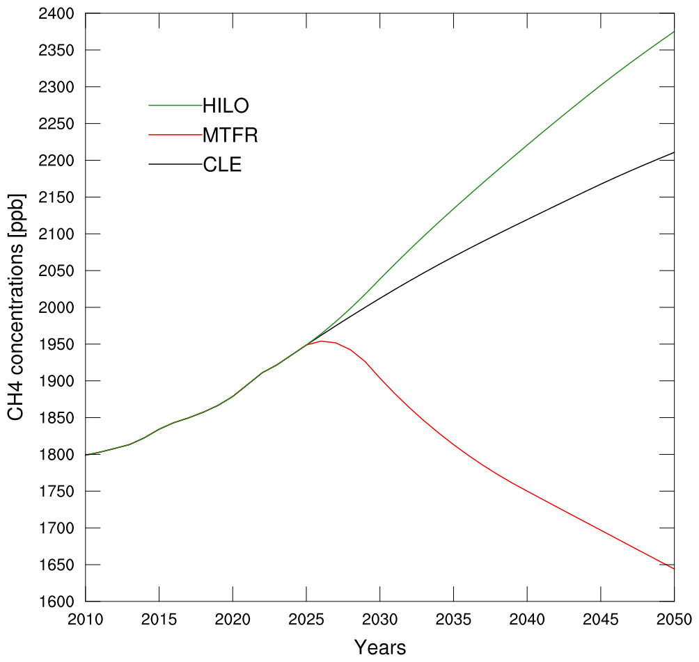
Figure 3 The trends in methane concentration under the CLE, MTFR, and HILO scenarios corresponding with the emissions from the GAINS LRTAP scenarios.

For the Transient Historical experiment, historical concentrations of methane are also provided as annual average surface mixing ratio in van Caspel and Fagerli (2025). For the historical period, these concentrations have been harmonised with the observations from the NOAA Global Monitoring Laboratory (Thoning et al., 2022). Modelling groups should fix the concentration of methane at their lower boundary to these values. Values are provided from 1998 to allow for up to five years of model spin-up.

5.6 Hydrogen

For all model experiments, groups must specify a global average surface mixing ratio of hydrogen of 530 ppb, equivalent to the present-day mixing ratio (Novelli et al., 1999). The GAINS LRTAP scenarios do not include emissions from a potential future hydrogen/ammonia economy, and other future projections of hydrogen emissions are too uncertain at this time.

5.7 Natural emissions and other emissions not specified in this experiment description

A key aim of the HTAP3-OPNS exercise is to minimise barriers to participation for modelling groups. As such, all modelling groups are free to choose whichever datasets are most convenient and appropriate for their model for natural emissions, and any other emissions not specified in this experiment description. We expect that each modelling group contributing to HTAP3-OPNS already has experience running their model and can make a judgement on the appropriate treatment of the emission sources and appropriate datasets required for their model simulations.

All groups are required to report their total emissions including both natural and anthropogenic emissions using the appropriate fields in the requested output data (Sect. 6) and additionally provide a description of the emission data sets or online calculations used for natural emissions or other emissions not specified in this experiment description in their simulations.

5.7.1 Emissions of Biogenic Volatile Organic Compounds

Each group is free to choose their own treatment of BVOC emissions. Ideally, BVOC emissions used in each model should be calculated online in a way consistent with the land cover and meteorology used in each model experiment, although we will also accept submissions from groups using offline BVOC emissions. Please note that reporting of both isoprene emissions and total BVOC emissions as model output fields are required in HTAP3-OPNS (Sect. 6).

5.7.2 Emissions of NO_x from lightning

Each modelling group is free to choose their own treatment of lightning NO_x emissions, including the overall magnitude of the lightning NO_x source. Ideally, groups should use the same treatment of lightning NO_x emissions as they have used in previously published evaluations of their respective models. Please note that reporting of lightning NO_x emissions as a model output field is required in HTAP3-OPNS (Sect. 6).

5.8 Land cover

There is no requirement in HTAP3-OPNS to use any specific land cover treatment. Each modelling group is free to choose whichever land cover treatment is most appropriate and convenient for their model, as long as it is broadly consistent with the period being simulated in each model experiment (Sect. 7). All groups are requested to report their land cover using the 16 generic land cover types defined for the AQMEII4 project (Galmarini et al., 2021).

For an offline treatment of land cover, we recommend the use of the LUH2 dataset (Hurtt et al., 2020), which provides detailed land cover patterns from 850–2100, and was used by modelling groups contributing to the CMIP6 model intercomparison project.

5.9 Meteorology and climate boundary conditions

Modelling groups are free to choose whichever meteorological or climate input data is most appropriate and convenient for their model, within the constraints of the relevant experimental specifications (Sect. 7).

For CTMs contributing to the Perturbation and Transient Historical experiments, this input consists primarily of archived meteorological fields (specified dynamics) from a reanalysis product. HTAP recommends that CTM groups use meteorological input data which they have previously used in published evaluations of their respective models.

For CCMs contributing to the Transient Future experiments, this input consists of sea surface temperature and ice cover data, as well as the concentrations of well-mixed greenhouse gases (except for methane, which must be taken from the GAINS LRTAP scenarios as either emissions or concentrations, Sect. 5.5). Groups are free to choose whichever source of input data is most convenient for their model. HTAP recommends that CCM groups use input datasets for the historical period and SSP2-4.5 corresponding to their own CMIP6 simulations (or equivalent).

6 Requested model output data

The full list of requested model output fields for HTAP3-OPNS is available in the supplement to this manuscript. This HTAP3-OPNS output table is based on the requested output for AerChemMIP (Collins et al., 2017), with several modifications specific to HTAP3-OPNS. The output request retains diagnostics identified as useful in previous model intercomparison and assessment exercises, both to maintain continuity with these exercises and to facilitate future analyses of the HTAP3-OPNS model archive that may extend beyond the analyses currently planned. In addition to the worksheets based on AerChemMIP, we have added a request for vertical profile output on model levels at the grid cells corresponding with the locations of ozonesone measurements from the TOAR2 HEGIFTOM dataset (Van Malderen et al., 2025) for the purposes of model evaluation.

All modelling groups are encouraged to provide as many of the HTAP3-OPNS diagnostic fields as possible from their simulations for all sets of experiments in HTAP3-OPNS. Diagnostic fields of particular importance, as well as new fields which have been added for HTAP3-OPNS, are described in this section below. A table of the full set of requested output fields is provided in the supplementary material to this manuscript. The format in which model output should be provided is described in Sect. 8.1.

For climate models contributing to the Transient Future experiments (Sects. 4.2 and 7.3), hourly fields should be saved in the first ten years (2010–2019) and last ten years (2040–2049) of each model run. All other models contributing to all other sets of experiments should save and report hourly fields for the full duration of each model experiment.

6.1 Hourly surface mixing ratio of ozone and other pollutants

In order to calculate policy-relevant ozone impact metrics, all groups are required to provide hourly averaged fields of the surface ozone mixing ratio at the lowest model level for all simulations in all sets of experiments. While this diagnostic was already included in the AerChemMIP output table, and is not new in HTAP3-OPNS, we emphasise the necessity of including this field for all models participating in all HTAP3-OPNS experiments.

In addition to the hourly mixing ratio of ozone, modelling groups are also strongly encouraged to provide hourly mixing ratio of PM_2.5 and NO₂ at the lowest model level, which will also be used in health impact assessment.

6.2 Ozone deposition and related fields

Ozone impacts on vegetation will be an important part of the analysis of HTAP3-OPNS. This will be jointly performed by HTAP in cooperation with ICP Vegetation (The International Cooperative Programme on Effects of Air Pollution on Natural Vegetation and Crops), a body of CLRTAP based at the UK Centre for Ecology and Hydrology. Ozone impacts on vegetation (primarily wheat crops and deciduous forests) will be determined using the PODyIAM (Phytotoxic Ozone Dose above threshold y for Integrated Assessment Modelling) metric using the DO3SE model (Emberson et al., 2007; Simpson et al., 2012).

Modelling groups who have implemented the DO3SE model (or equivalent methods for calculating the PODyIAM metrics) in their systems are encouraged to directly provide daily accumulated values of the relevant PODyIAM metrics. Crop impacts will be calculated from POD3IAM, and forest impacts will be calculated from POD1IAM. A detailed description for the calculation of these metrics is given in CLRTAP (2023). Groups who are able to calculate PODyIAM metrics should provide both POD1IAM and POD3IAM at daily resolution on a longitude/latitude grid.

All groups (including groups which calculate and provide the PODyIAM metrics) should provide hourly values of the following parameters (where available) as a high priority, which will be used to calculate the PODyIAM metrics offline:

• Hourly mean 2D (longitude, latitude) output:

  • –

    Mixing ratio of ozone at the lowest model level (also requested in Sect. 6.1),

  • –

    Ozone deposition flux,

  • –

    Ozone deposition velocity,

  • –

    Aerodynamic resistance as used in the deposition calculation.

  • –

    Near-surface air temperature,

  • –

    Near-surface relative humidity,

  • –

    PPFD (Photosynthetic Photon Flux Density).

    • –

      If this is not available, it can be calculated offline based on location and time.

• Daily mean 2D (longitude, latitude) output:

  • –

    soil_moisture_content.

• Monthly mean 2D (longitude, latitude) output:

  • –

    soil_moisture_content,

  • –

    soil_moisture_content_at_field_capacity,

  • –

    Land cover maps including all vegetation types used in the model runs using the generic land cover types defined for the AQMEII4 exercise (Galmarini et al., 2021).

Groups with the capacity to do so should also provide the soil_moisture_content variables at the vertical resolution of their soil model in addition to the vertically integrated soil moisture variables mentioned above (CF names moisture_content_of_soil_layer and moisture_content_of_soil_layer_at_field_capacity).

In addition to the requested data, all groups are also requested to provide detailed information about their ozone deposition schemes, in particular about whether and how soil moisture is included in the calculation of the deposition velocity.

6.3 Total deposition

The WMO MMF-GTAD exercise (https://community.wmo.int/en/activity-areas/gaw/science-for-services/mmf-gtad, last access: 1 September 2026) requires comprehensive information on total atmospheric deposition at monthly resolution. Modelling groups contributing to the HTAP3-OPNS experiments are encouraged to fully implement and provide these model diagnostics for all sets of experiments. Total deposition output is required for models contributing to the Transient Historical experiments, since this set of experiments will provide the model output for the MMF-GTAD exercise.

The requested deposition fields from the HTAP3-OPNS output table (monthly mean output) are as follows:

• dry deposition rate of O₃,

• dry deposition rate of dry aerosol total organic matter,

• wet deposition rate of dry aerosol total organic matter,

• dry deposition rate of black carbon aerosol mass,

• wet deposition rate of black carbon aerosol mass,

• dry deposition rate of seasalt,

• wet deposition rate of seasalt,

• dry deposition rate of dust,

• wet deposition rate of dust,

• dry deposition rate of SO₂,

• dry deposition rate of SO₄,

• wet deposition rate of SO₄,

• wet deposition rate of SO₂,

• dry deposition rate of NH₃,

• dry deposition rate of NH₄,

• wet deposition rate of NH₄,

• wet deposition rate of NH₃,

• dry deposition rate of NO_y,

• wet deposition rate of NO_y incl aerosol nitrate,

• dry deposition rate of organic nitrate,

• wet deposition rate of organic nitrate incl aerosol organic nitrate.

Except for the deposition diagnostics for organic nitrates, all the requested deposition fields were already included in the AerChemMIP output tables. The organic nitrate deposition diagnostic fields were added to the HTAP3-OPNS output table at the request of the WMO MMF-GTAD exercise.

6.4 Ozone and other chemical budget terms

The ensemble of models contributing to the various sets of experiments of HTAP3-OPNS represents an opportunity to explore inter-model differences in ozone production and loss terms which may help to explain the inter-model differences in simulated ozone. Modelling groups with the capacity to provide chemical flux diagnostics are encouraged to provide appropriate output which can be used to construct detailed ozone budgets.

The AerChemMIP output tables already contain variables diagnosing the monthly mean ozone production and loss terms in units of cm⁻³ s⁻¹. For HTAP3-OPNS we ask for modifications to the ozone loss diagnostic, and several additional diagnostic fields to enable more detailed investigation of the ozone budget and comparison of tropospheric chemistry across participating models:

• The ozone loss diagnostic o3loss should be modified to include O_x loss due to halogen chemistry for models which include this chemistry.

• An additional diagnostic primo3loss is requested for primary ozone loss (as the tendency due to reaction between O(¹D) and water vapour).

• Additional diagnostics do3chm and tropdo3chm are requested for the change in ozone across the chemical timestep.

• An additional diagnostic oxprodo2photo is requested for the production rate of O_x due to the photolysis of molecular oxygen.

• An additional diagnostic ohprod is requested for the total OH production rate, the OH production from all reactions producing OH, including rapid HO_x interconversion.

• An additional diagnostic ohloss is requested for the total OH loss rate, the OH loss from all reactions consuming OH, including rapid HO_x interconversion.

• An additional diagnostic prodco is requested for the secondary chemical production of CO.

The standard 2D diagnostics tropoz and toz are also requested as monthly averages. The variable toz is the total ozone column, while the tropospheric ozone column field (tropoz) is calculated using a dynamically varying online pressure tropopause (ptp) according to the WMO thermal tropopause definition. Both should be output on the model native lat/lon grid.

In addition to the extra diagnostic terms, we request all groups to provide a machine-readable file containing their model chemical mechanism to assist in the interpretation of the diagnostic terms. An overview of the planned analyses using these diagnostics is given in Sect. 8.2.6.

6.5 Boundary conditions for regional models

Since it will not be possible for HTAP to centrally host the large amount of data required for regional boundary conditions, data exchange between global and regional modellers should be organised directly between interested global and regional modellers. HTAP will help with coordination of this exchange. Further details on boundary conditions for regional modellers are given in Sect. 7.2.1.

6.6 Common radiation calls for Earth System Models

To quantify the effects of the individual emission components on the radiative budget we propose to include additional diagnostic double calls into the CCM model simulations. For aerosols we suggest applying the Ghan method (Ghan, 2013) and include an additional diagnostic “aerosol free” radiation call to quantify the instantaneous radiative forcing due to aerosol–radiation interactions. This diagnostic does not include radiative effects mediated by aerosol–cloud interactions. Similarly, we propose to include an additional diagnostic radiation call with an ozone climatology instead of the interactive ozone (see Collins et al., 2025). These double calls should be provided to allow diagnosis of the instantaneous radiative forcing (IRF). Models which can also provide a stratospheric adjusted radiative forcing (SARF) are invited to provide these fields in addition.

7 Experimental setup

For all experiments in each of the three sets, participating modelling groups have the flexibility to configure their model as they see fit (e.g. grid resolution, meteorological/climate boundary conditions, natural emissions, chemical mechanism, spinup time, etc. …), as long as they adhere to the requirements for the use of specific input datasets as shown in Table 1 and described in Sect. 5, and provision of output fields described in Sect. 6. Modelling groups are requested to document their model configuration as described in Sect. 7.5.

7.1 Perturbation experiments

All experiments in this set consist of year-long model simulations performed by global CTMs or CCMs with specified dynamics, land cover, biomass burning, and natural emissions for a common meteorological base year (2015). Anthropogenic emissions excluding agricultural waste burning for all model runs are based on GAINS LRTAP emissions (Sect. 5.1). Biomass burning emissions including agricultural waste burning are based on the GFAS4HTAP dataset (Sect. 5.3). Methane concentrations corresponding with the emissions from the three GAINS LRTAP scenarios (CLE, MTFR, and HILO, Sect. 5.5) are specified as concentration boundary conditions in all runs of this set of experiments. This set of experiments has two primary goals:

• Direct simulation of single years of the GAINS LRTAP scenarios (2015 and 2040) as a complement to the Transient Future experiments and for the provision of lateral boundary conditions to regional model simulations.

• Production of source/receptor relationships for hemispheric air pollution in 2040 for the construction of the HTAP3 ensemble emulator (Sect. 8.2.2).

Model groups should ensure that their model is appropriately spun up in each case. In general, we recommend at least 6 months of spin-up for each run (beginning in July and using the same emissions and meteorology as the simulation itself, if 2014 meteorology is not available for spinup then it is acceptable to use 2015 meteorology for the spinup), assuming that initial conditions are chosen appropriately, as recommended below. A good test for sufficient spin-up would be to compare the December output from the spin-up period with the December output from the delivered model output and to check for the absence of any chemical drift.

The runs in this set of experiments are shown in Table 2 (global perturbation experiments with global CTMs) and Table 3 (regional perturbation experiments with global CTMs) and described in more detail below.

Table 2 Overview and prioritisation of the global perturbation experiments in HTAP3-OPNS.

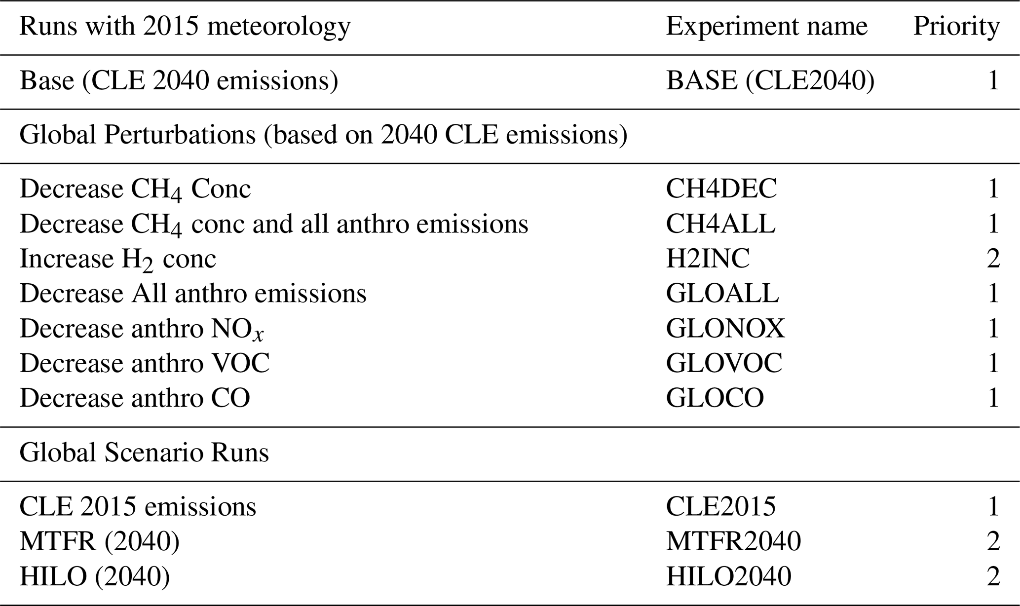
Table 3 Overview and prioritisation of the regional perturbation experiments (run with global CTMs) in HTAP3-OPNS. The number in each cell corresponds with the priority of the corresponding simulation. Priority 1 and 2 experiments are shown in bold type.

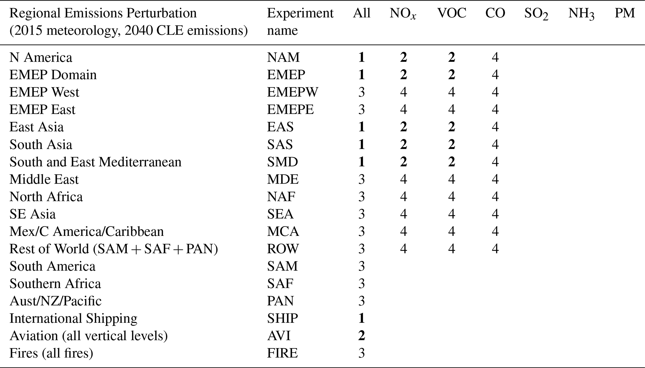
All model runs should be performed using 2015 meteorology, biomass burning emissions, natural emissions, and land cover. Recognising that most modelling groups will not have the capacity to perform a large number of simulations, the model runs in Tables 2 and 3 are prioritised according to their usefulness for constructing the HTAP3 ensemble emulator. There are 14 runs with a priority of 1, and another 10 runs with a priority of 2. Remaining runs are given either priority 3 or 4 or not requested at all. Construction of reliable model emulators requires contribution of results to priority 1 runs and would benefit from results for priority 2 runs; priority 3 and 4 runs provide useful additional information on regional and species contributions but are less essential.

All groups contributing simulations to this set of experiments are required to perform the base simulation, which uses GAINS LRTAP CLE 2040 emissions and methane concentrations, and another simulation using GAINS LRTAP CLE 2015 emissions and methane concentrations. The CLE2040 simulation will form the basis for all perturbation runs in this set, while the CLE2015 run will be used for model evaluation as well as to evaluate the change in global air quality between 2015 and 2040.

For the spin-up of the CLE2015 and CLE2040 simulations, we recommend initialising the model with archived 3D concentrations from an existing present-day simulation, but with 3D fields of methane and hydrogen set to the same values as the respective specified surface concentrations from each scenario. We recommend using the same initial conditions as CLE2040 for all other perturbation runs, except where otherwise specified. As mentioned above, we recommend six months of spin-up for each model run, but each group should ensure that their model is appropriately spun-up for each run.

7.1.1 Direct scenario experiments

There are four direct scenario runs requested in this set of experiments: CLE2015; CLE2040; MTFR2040; and HILO2040. These runs will be used to assess future global air quality under the GAINS LRTAP scenarios and as a source of boundary conditions for regional model simulations (Sect. 7.2.1).

The CLE 2015 and CLE 2040 runs have priority 1 because they are used respectively for model evaluation and as the base case for source/receptor runs. All groups contributing to the Perturbation experiments should perform these two runs.

The MTFR2040 and HILO2040 runs have priority 2 because they do not contribute directly to the construction of the HTAP3 ensemble emulator. However, global modelling groups providing lateral boundary conditions for regional model simulations should perform both of these runs as a matter of high priority. Other global modelling groups with additional resources and an interest in the assessment of these scenarios are also encouraged to perform these runs as long as they also perform the 14 priority 1 runs (Tables 2 and 3).

For the spin-up of all direct scenario simulations, we recommend initialising the model with archived 3D concentrations from an existing present-day simulation, but with 3D fields of methane and hydrogen set to the same values as the respective specified surface concentrations from each scenario.

As noted in Sect. 3, all emission fluxes except for methane for the HILO scenario are taken from the MTFR scenario. As also noted in Sect. 5.5, methane concentrations for the HILO run in this set of experiments are calculated based on methane emissions from the CLE scenario, but the resulting methane concentrations are not identical between CLE and HILO. Groups performing the HILO2040 run should take care to use methane concentrations from Met.no for the HILO scenario (Sect. 5.5).

7.1.2 Global perturbation experiments

Global perturbation runs are performed by decreasing the specified emissions or surface concentrations by 20 % relative to the base run, as for previous HTAP assessments. There are six priority 1 global perturbation runs:

• CH4DEC. The global methane concentration boundary condition is reduced by 20 %.

• CH4ALL. The global methane concentration boundary condition and all anthropogenic (including shipping and aviation) emissions (NO_x, NMVOC, CO, SO₂, NH₃, and all PM species) are reduced by 20 % globally. Biomass burning emissions (including agricultural waste burning) and natural emissions are not changed.

• GLOALL. All anthropogenic (including shipping and aviation) emissions (NO_x, NMVOC, CO, SO₂, NH₃, and all PM species) are reduced by 20 % globally. Biomass burning emissions (including agricultural waste burning), natural emissions, and methane concentrations are not changed.

• GLONOX. All anthropogenic emissions (including shipping and aviation but excluding agricultural waste burning) of NO_x are reduced by 20 %.

• GLOVOC. All anthropogenic emissions (including shipping and aviation but excluding agricultural waste burning) of NMVOC are reduced by 20 %.

• GLOCO. All anthropogenic emissions (including shipping and aviation but excluding agricultural waste burning) of CO are reduced by 20 %.

In addition to the priority 1 global perturbation runs, there is also a priority 2 global perturbation run H2INC, in which the hydrogen concentration boundary condition is increased by 20 %. Groups with the additional resources to perform this run are encouraged to do so, which will allow the HTAP3 ensemble emulator to include the atmospheric response to future changes in hydrogen.

For the CH4DEC and CH4ALL simulations, we recommend applying the 20 % reduction in methane concentrations to the 3D initial conditions as well as to the surface boundary conditions to reduce the need for additional spin-up time. Similarly, for the H2INC simulation, we recommend applying the 20 % increase in H₂ concentrations to the 3D initial conditions as well as to the surface boundary condition.

7.1.3 Regional and sectoral perturbation experiments

There are six priority 1 runs with global models which include regional or sectoral emission perturbations of −20 % relative to the base run of all anthropogenic species (NO_x, NMVOC, CO, SO₂, NH₃, and all PM species). The source regions for the perturbation experiments are shown in Fig. 4 and are available for download from Zenodo (Butler, 2025). Please make sure to use version 4 of this dataset. Since the work has been designed to support the revision of the CLRTAP Gothenburg Protocol, the primary focus is the Northern Hemisphere. For the five regional perturbation runs, only the land-based anthropogenic emission sectors should be perturbed. No perturbation should be applied for aviation emissions, international shipping emissions, biomass burning emissions (including agricultural waste burning), or natural emissions.

• NAMALL. Emissions are reduced by 20 % over the North American source region.

• EMEPALL. Emissions are reduced by 20 % over the EMEP source region.

• EASALL. Emissions are reduced by 20 % over the East Asia source region.

• SASALL. Emissions are reduced by 20 % over the South Asia source region.

• SMDALL. Emissions are reduced by 20 % over the Southern Mediterranean source region.

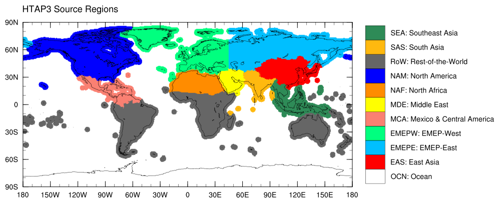
Figure 4 The HTAP3 source regions.

In addition to the priority 1 regional perturbation runs, we also request with priority 1 the SHIPALL perturbation run, in which all emissions from the international shipping sector (regardless of location) are reduced by 20 %.

There are an additional 10 regional perturbation runs of priority 2 corresponding to the five major source regions with −20 % perturbations of anthropogenic emissions (excluding aviation, all biomass burning sectors, and natural emissions) of individual pollutant species (5 NO_x perturbation runs and 5 NMVOC perturbation runs):

• NAMNOX and NAMVOC,

• EMEPNOX and EMEPVOC,

• EASNOX and EASVOC,

• SASNOX and SASVOC,

• SMDNOX and SMDVOC.

For groups which have performed at least the 14 priority 1 runs (Tables 2 and 3), and ideally also the 10 priority 2 runs, there are an additional 12 priority 3 regional or sectoral perturbation runs which would be of use in constructing the HTAP3 ensemble emulator:

• EMEPWALL and EMEPEALL. these runs help with disaggregation of the EMEP source region into its western and eastern parts.

• NAFALL and MDEALL. these runs help with disaggregation of the SMD source region into its component parts.

• ROWALL, SAMALL, SAFALL, and PANALL. these runs complete the coverage of all global source regions.

• AVIALL and FIREALL. these runs help to quantify the response of air pollution to emissions from aviation and biomass burning respectively.

Runs listed as priority 4 in Table 3 are useful in the construction of the HTAP3 ensemble emulator. Due to the large number of runs of priority 1, 2, and 3, we do not expect many groups to perform runs of priority 4. However, groups with a special interest in priority 4 perturbation runs are encouraged to perform these and submit them to the data archive if they have completed at least the 14 priority 1 runs, and ideally also the 10 priority 2 runs.

7.2 Global to regional downscaling of GAINS LRTAP scenarios

A major motivation for the work in HTAP3-OPNS is the revision of the CLRTAP Gothenburg Protocol, which regulates the emissions of ozone precursors and particulate matter in the UNECE region. Assessment of the GAINS LRTAP scenarios using high resolution regional models for Europe and North America is therefore an important part of HTAP3-OPNS. Depending on interest from regional modellers simulating other domains, there may also be demand for boundary conditions for other regions. For compatibility with global specified-dynamics simulations in HTAP3-OPNS, regional simulations should be performed using meteorological input from the common base year (2015).

7.2.1 Global simulations providing boundary conditions for regional models

Lateral boundary conditions for regional model simulations will be taken from the global simulations of CLE2015, CLE2040, MTFR2040, and HILO2040 (Sect. 7.1.1). Global modellers performing these four simulations during the course of HTAP3-OPNS are encouraged to save output of key model species at high temporal resolution (at least 6 hourly) and 3D spatial resolution (globally or at the coordinates of regional model boundaries) in a format accessible for regional modellers. Given that HTAP will not have the resources to store these boundary conditions centrally on the AeroCom server, these data are not part of the formal data request. Global modelling groups providing boundary conditions for regional models are requested to host these data themselves and make them available to regional modellers.

HTAP will make efforts to identify regional modellers interested in downscaling the GAINS LRTAP scenarios for their region using boundary conditions from HTAP3-OPNS global runs. HTAP will work to connect regional modellers with global modellers and help to identify the key species which must be saved from global simulations, and the coordinates at which these species should be saved.

NCAR will perform global simulations with the CAM-chem model and host global 3D 6-hourly output of the species listed here: https://wiki.ucar.edu/display/camchem/CESM 2.2: Species saved in boundary condition files (last access: 1 September 2026). These species should be especially suitable for regional models using chemical mechanisms related to the MOZART mechanism as used in CAM-chem.

The CLRTAP MSC-W will perform global simulations with the EMEP model and host 6-hourly output at the edges of the CAMS and EMEP domains.

The IFS-COMPO operated within the Copernicus Atmosphere Monitoring Service (Peuch et al., 2023) model will also undertake the core global simulations and make them available. As far as the European domain is concerned, the operational character of CAMS is making the IFS-COMPO a well established and easy to use source of boundary conditions for regional modellers.

7.2.2 Regional model simulations for Europe

Several regional modelling groups with a focus on Europe have expressed an interest in performing simulations through fora such as the CLRTAP Task Force on Measurements and Modelling (TFMM) and the Copernicus Atmosphere Monitoring Service (CAMS).

European regional modellers are encouraged to perform simulations for the EMEP domain where possible, otherwise for the CAMS domain. Groups performing simulations using the CAMS domain must make sure to simulate the entire geographical extent of the CAMS domain.

All regional model input data should be harmonised as closely as possible with the descriptions given in Sect. 5. Meteorological input data should correspond with the base year (2015) for all simulations. Anthropogenic emissions excluding agricultural waste burning should be taken from the relevant GAINS LRTAP scenarios (Sect. 5.1). Regional model simulations should not specify methane emissions within their simulation domain but rather specify methane concentrations at their lateral boundaries. Biomass burning emissions including agricultural waste burning should be taken from the GFAS4HTAP dataset (Sect. 5.3) for 2015 for all simulations. Natural emissions should also correspond with the year 2015. All other aspects of model configuration are left to the discretion of the regional modelling groups.

A summary of the regional model simulations for Europe is given in Table 4. Five simulations are requested from each contributing modelling group. Simulations 1–3 use the same emission scenario in both the global and regional models. Simulation 4 uses MTFR emissions for air pollutants in both the global and regional domains and boundary conditions from the global HILO scenario. Simulation 5 uses boundary conditions from CLE2040, but emissions from all land-based anthropogenic emission sectors (excluding aviation and international shipping) in the EMEP West source region (Fig. 4 and Butler, 2025) within the regional model domain are replaced with the corresponding emissions from the MTFR2040 scenario. All regional simulations should cover the full meteorological year 2015.

Table 4 Regional model simulations for Europe in HTAP3-OPNS.

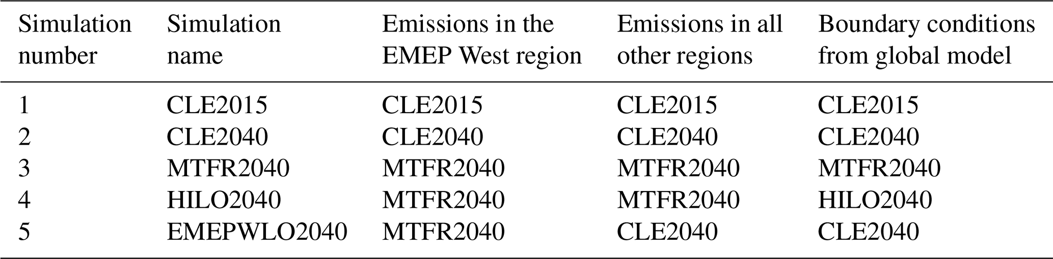
It is anticipated that several different sets of boundary conditions from different global models will be available for these simulations (Sect. 7.2.1). Regional modelling groups are free to choose the most convenient dataset and encouraged to choose the global model output which most closely corresponds to their chemical mechanism. Groups with the resources to perform additional simulations are encouraged to perform the same set of five regional simulations using alternative boundary conditions.

Regional modelling teams should format their model output according to the instructions in Sect. 8.1 before uploading their data to the AeroCom server, taking care to include the fields which are indicated to be of high priority for HTAP3-OPNS.

7.3 Transient future experiments

In this set of experiments, transient model simulations will be performed by CCMs with the GAINS LRTAP scenarios (Sect. 5.1) from 2010–2050 and the future fire emissions described in Sect. 5.2. The 10-year period 2010–2019 will be used to determine the baseline conditions for the present day (corresponding to the year 2015), and the 10-year period 2040–2049 will be used to determine the conditions corresponding to the end of the scenarios. The full transient timeseries of model output will be used to determine the model responses to changing emissions.

7.3.1 Scenarios and prioritisation

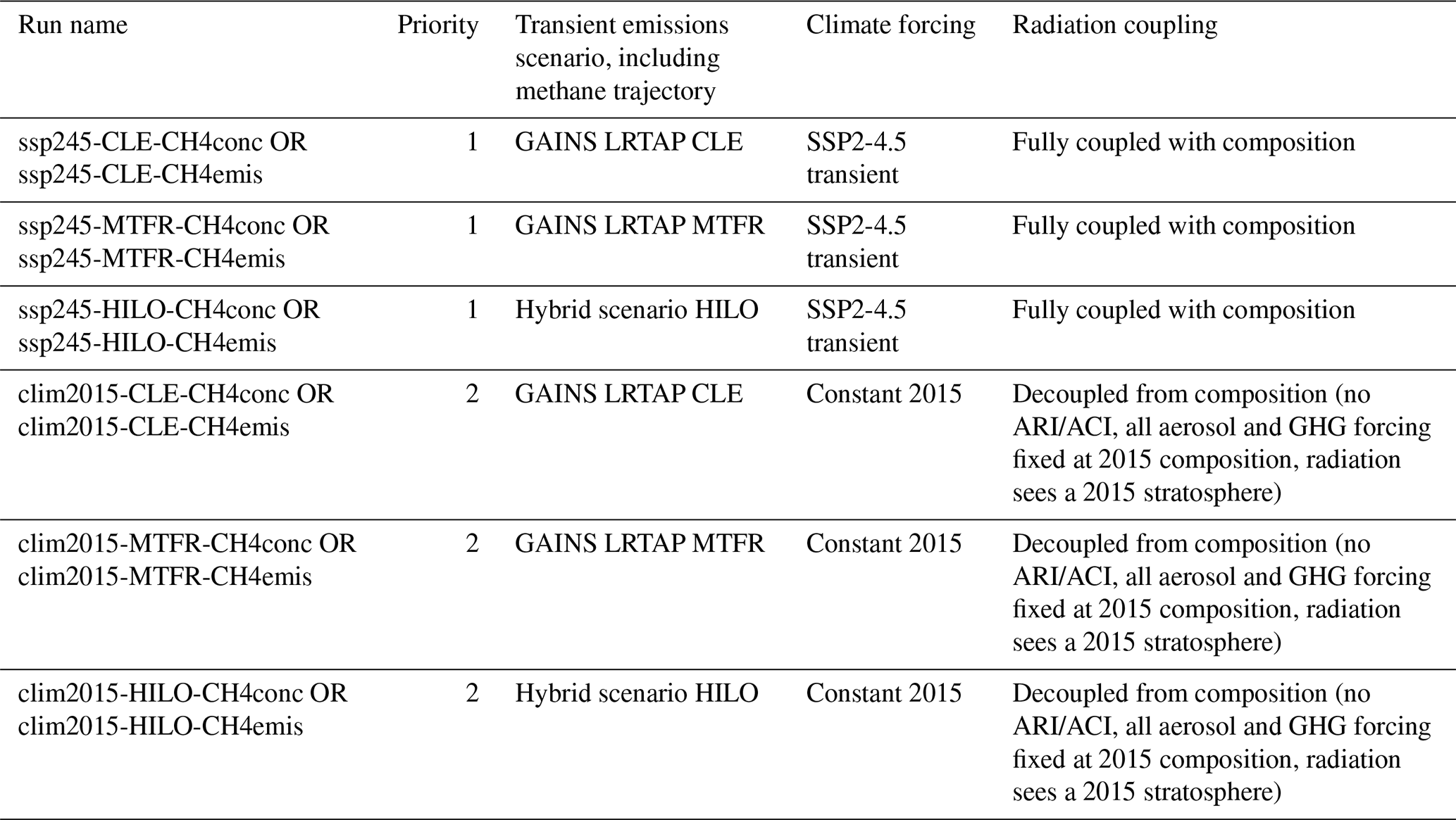
All CCM groups contributing to the Transient Future Scenarios experiments are requested to run at least the three core scenarios: CLE; MTFR; and HILO, as described in Sects. 3 and 5.1. All three of these scenarios should be run with climate forcing corresponding to SSP2-4.5. Comparison of these three scenarios with each other will directly inform the Gothenburg Protocol revision process with an understanding of future air quality under these three emission pathways. In addition to the three core scenarios, CCM groups with the resources to run an additional three simulations are requested to run the same three core emission scenarios, but with constant fixed climate forcing corresponding to the year 2015. Comparison of the fixed 2015 climate forcing simulations with the transient-forcing SSP2-4.5 simulations will allow calculation of the climate penalty on air pollution under the GAINS LRTAP scenarios.

Modelling groups with the capability of performing methane emissions-driven simulations are strongly encouraged to do this for their contributions to the Transient Future Scenarios experiments. Surface methane mixing ratios for concentration-driven model runs are described in Sect. 5.5). As noted in Sect. 5.5, the methane concentration pathways in each of the three scenarios are distinct. Groups may submit both emissions-driven and concentration-driven simulations for each scenario if they wish. A summary of the six requested runs is given in Table 5.

Table 5 Chemistry-climate model simulations for the Transient Future experiments in HTAP3-OPNS.

7.3.2 Chemistry-climate model setup

Groups are encouraged to use any version of their model which they think is appropriate, although we recommend that they use their CMIP6-AMIP configuration. Model output of the fields described in Sect. 6 in the format described in Sect. 8.1 should be reported for the years 2010–2050, with the exception of hourly surface fields, which should only be reported for the first ten years (2010–2019) and last ten years (2040–2049) of each model experiment. Model runs should begin from a sufficiently spun-up state in the simulation year 2010. We leave the details of model spin-up to each modelling group.

7.3.3 Climate forcing data

Climate forcing data for each run consists of the following fields:

• Sea surface temperatures,

• Ice cover,

• Land cover (unless using a dynamic land model),

• Concentrations of long-lived greenhouse gases (except for methane, which should be specified from the GAINS LRTAP scenarios),

• Ozone depleting substances.

For the “ssp245” runs, the climate forcing fields should be taken from the CMIP6 SSP2-4.5 forcing data. Fields not directly specified in SSP2-4.5 (SST and ice cover data) could be taken from a previous run of a fully coupled ESM forced with SSP2-4.5. As the SSP2-4.5 forcing data begins in 2015, modelling groups will need to perform the first part of their ssp245 simulations up until 2014 (including the spin-up) with historical forcing data. We recommend that groups begin their spin-up by branching from an existing CMIP6 historical simulation of their model, substituting the GAINS LRTAP scenarios from the branching year. The choice of branching year for sufficient spin-up is left to the judgement of each modelling group.

For the “clim2015” runs, the climate forcing fields, CO2 concentrations, other long-lived GHG (apart from methane), and ozone depleting substances should be taken from the year 2015 of an appropriate SSP2-4.5 dataset and kept constant throughout the entire simulation (including sufficient spin-up). All aspects of radiative forcing should also be kept constant at 2015 levels; this means that the evolving simulation of atmospheric composition (including methane, ozone, particles, and stratospheric composition) in response to the GAINS LRTAP scenarios should be decoupled from the model radiation scheme in the clim2015 simulations, with the model radiation seeing 2015 composition. SST and ice cover data should be taken from a 10 year (2005–2014) average of a previous fully coupled historical run of a fully coupled ESM. Land cover data should be kept constant in the clim2015 runs.

We note that the updated versions of the GAINS LRTAP scenarios will diverge from one another from the year 2025. Where appropriate, modelling groups are advised to branch their future simulations from this year to save storage and computational resources.

7.4 Transient historical experiment

This run should be performed with specified dynamics, the HTAPv3.2 global mosaic anthropogenic emissions (Sect. 5.4), the GFAS4HTAP biomass burning emissions (Sect. 5.3), and surface methane concentrations from the NOAA network (Sect. 5.5) for the period 2003–2020. Groups not in the position to perform the full time series should focus on the latter part of the period and include at least the year 2015 in their simulation. Groups performing this simulation are required to include total deposition output in their data submission (Sect. 6.3), as this will be provided to the WMO MMF-GTAD exercise.

7.5 Documentation of model configuration

Given the many choices left at the discretion of modelling groups in the configuration of models for HTAP3-OPNS, all groups are requested to document all choices made during model configuration to aid in the interpretation of results. This documentation should be uploaded along with the initial data delivery (Sect. 8.1). A summary will be added to the permanent archive of model results (Sect. 8.3).

7.5.1 All contributing models

All models should document the following details:

• Model version used,

• Reference to the most recent model documentation,

• Horizontal and vertical model resolution,

• Machine-readable gas phase chemical mechanism,

• Treatment of secondary inorganic aerosol, including nitrate aerosol,

• Treatment of secondary organic aerosol,

• Treatment of wet and dry deposition, including the treatment of soil-moisture effects on ozone deposition,

• Land cover dataset (or land surface model),

• Chemical speciation profiles for all lumped emitted species,

• Temporal emission profiles for all emitted species,

• Vertical injection profiles for all emitted species,

• Description of natural emission sources and any other emission sources not specified for HTAP3-OPNS, including the treatment of BVOC, emissions from soils, and lightning NO_x emissions,

• Length of spin-up.

7.5.2 Chemical transport models

Global and regional CTMs should include the following in their documentation:

• Source of meteorological input data,

• Choice of boundary condition data for regional CTMs, including the global model used.

7.5.3 Chemistry-climate models

Chemistry-climate models should include the following in their documentation:

• Source of SST and ice cover data,

• Methane flux adjustment (for CCMs driven with methane emissions),

• Any deviations from the prescribed SSP2-4.5 forcing.

8 Data handling

8.1 Initial delivery of data

Model output from HTAP3-OPNS as specified in the data request (Sect. 6) will be stored on the AeroCom server (https://aerocom.met.no/, last access: 1 September 2026). All groups contributing model output to HTAP3-OPNS must request an account on this server linked to the HTAP3-OPNS project. Data must be uploaded to the AeroCom server on a regular lat/lon grid. Model grids based on other projections or unstructured grids should be regridded by each modelling group to a regular lat/lon grid at an equivalent resolution to the native model grid before being uploaded to the AeroCom server.

Data must be submitted in the CF-compliant netCDF format with file names based on the following convention:

• htap3opns_<ModelName>_<ExperimentName-PerturbationRealisation>_< DataRequestSheet>_<VariableName>_ <Period>.nc

where:

• <ModelName> should be chosen such that model name, model version, and possibly the institution can be identified. No underscores (_) are allowed in <ModelName>, use (−) instead. Restrict <ModelName> to max 20 characters.

• <ExperimentName> = will either be TransientHistorical, or follow the naming conventions introduced for each experiment in Sect. 7.1, 7.2, and 7.3. For the various emissions perturbation runs, PerturbationRealisation will be 5–8 letters (3–5 indicating the region of perturbation and 2–3 indicating the pollutants or sector decreased) based on the experiment matrix in Tables 2 and 3. For example, CLE2040-GLOALL is used to indicate a 20 % decrease in anthropogenic emissions globally; CLE2040-NAMNOX is used to indicate a 20 % decrease in anthropogenic NO_x emissions from North America; and CLE2040-EMEPWVOC is used to indicate a 20 % decrease in anthropogenic NMVOC from the EMEP West region.

• <DataRequestSheet> refers to the name of the sheet in the data request in which the variable was requested = aerfixed, aermonthly-3d, aermonthly-2d, aerdaily, aerhourly, aerzonal-vert, aerzonal, ModelLevelAtStations.

• <VariableName> = are the HTAP variable short names in the requested output spreadsheet discussed in Sect. 6 above. An example of a variable short name is: vmro3.

• <Period> = year of simulation.

8.2 Analysis of model experiments

During the analysis phase of HTAP3-OPNS, access to the submitted model output will be restricted to users of the AeroCom server who have requested access to the HTAP3 project. Groups who have not contributed model output, but who are interested in contributing to the analysis are welcome to contact the HTAP leadership team. The HTAP leadership team will organise regular meetings for all participants in the project to gauge the progress of model simulations and to coordinate the associated analyses. A non-exhaustive summary of some expected analysis is given below in this section.

8.2.1 Model evaluation

Comparison of model results with observations is vital for determining the degree to which models are capable of simulating the historical past and providing confidence in their ability to make future projections. The requested model output fields in HTAP3-OPNS (Sect. 6) include hourly surface (2D) values of ozone, NO₂, PM₁₀, PM_2.5, and other species which are routinely measured at surface sites. With its focus on the impacts of air pollution on human health and ecosystems, the evaluation of model results against surface observations will be of high priority. The harmonised datasets collected and made available by the TOAR-II (Tropospheric Ozone Assessment Report phase 2, https://toar-data.org/, last access: 1 September 2026) will be especially useful for the evaluation of ground-level and tropospheric ozone. In addition to hourly surface concentrations, the requested model output also includes other fields which can be used in model evaluation, such as Aerosol Optical Thickness (AOT) at different wavelengths, deposition fields, and monthly mean 3D concentrations. Results from the CLE2015 CTM experiment (Sect. 7.1.1), the first 10 years of the transient future experiment (Sect. 7.3), and the full transient historical experiment (Sect. 7.4) will deliver output suitable for evaluation.

8.2.2 Source-receptor relationships and emulator development

The source-receptor relationships from the perturbation experiments (Sect. 7.1) will allow the construction of an ensemble emulator for rapid assessment of ozone, PM, and the deposition of N and S under alternative future emission scenarios. Previous HTAP assessments have demonstrated the value of this approach for quantifying surface ozone concentration changes across a wide range of future scenarios along with an estimate of the associated uncertainty as represented by the spread of responses across contributing models (Turnock et al., 2018; Wild et al., 2012). The approach allows incorporation of the nonlinearity in model responses and provides a valuable tool to guide policy development.

Use of a 2040 baseline will allow exploration of source-receptor relationships under future conditions, permitting a more robust assessment of the effectiveness of mitigation measures around this policy-relevant target year. Use of the emulator will allow rapid assessment of additional mitigation scenarios in addition to the CLE and MTFR scenarios in support of the revision of the Gothenburg Protocol. Groups are encouraged to submit results for as many of the runs as they can, but to focus in particular on runs defined as high priority to permit reliable emulation of their model.

8.2.3 Assessment of future air quality

An assessment of the air quality under the GAINS LRTAP future scenarios is a fundamental goal of HTAP3-OPNS. The transient future experiments (Sect. 7.3) will provide a direct assessment of future air quality using state-of-the-art Chemistry-Climate Models both with and without the effects of climate change. The direct scenario experiments (Sect. 7.1.1) will add to this with Chemical Transport Model simulations of air quality in 2040. The CTM ensemble emulator (Sect. 8.2.2) will also allow the attribution of future air quality to specific source regions. Analyses of future air quality using results generated in HTAP3-OPNS will be coordinated by TF-HTAP and a synthesis report will be written by the TF-HTAP leadership team for presentation to the Convention on Long-Range Transboundary Air Pollution.

8.2.4 Ozone impact on health

The collection of hourly surface ozone mixing ratio from all participating models (Sect. 6.1) will allow the calculation of health impact metrics based on the MDA8 (Maximum Daily 8 h Average) ozone mixing ratio at the year and seasonal levels to compute the appropriate exposure indicators (e.g. peak season ozone, SOMO35). Such metrics will be used to estimate premature mortality, years of life lost attributable and other health outcomes attributable to ozone exposure by means of concentration-response functions (Huangfu and Atkinson, 2020; Murray et al., 2020; Kasdagli et al., 2024) associated with all-cause or specific causes of mortality (e.g. respiratory disease or chronic obstructive pulmonary disease). In this way it will be possible to link the measures and assumptions in the studied scenarios, especially those concerning the influence of methane emissions on ozone concentrations, with their implications for health. The information about regional emissions and activity sectors will be used to provide insights about the allocation of health impacts to their sources (Belis and Van Dingenen, 2023). In addition, the health impacts of other pollutants such as PM_2.5 and NO₂ and their implication for this analysis will be also explored.

8.2.5 Ozone impact on vegetation

This analysis was briefly introduced in Sect. 6.2. HTAP and ICP Vegetation will calculate the PODyIAM metrics using a standardised land cover dataset. The land cover provided by the modelling groups will be used to better understand the provided deposition fluxes and as a consistency check with the standardized dataset used by ICP Vegetation. This calculation will also use the provided hourly temperature, humidity, and PPFD where available. The availability of daily average soil moisture output will provide additional flexibility for the PODyIAM calculation. Impacts of ozone deposition on vegetation co-occur with effects of changing climates (e.g., higher temperatures and in some regions more frequent and intense drought events). The proposed simulations will allow us to unravel interactions between changing climatic conditions and ozone deposition and their impacts on vegetation.

8.2.6 Ozone budget analysis

Several analyses are planned using the additional chemical diagnostics requested in Sect. 6.4. The addition of halogen loss reactions for ozone will help with closing the ozone budget. The addition of the primary ozone loss term, which is driven by photolysis, will help to separate the role of model physics from the role of model chemistry in ozone loss. The addition of the OH production term will enable comparison of primary and secondary OH production across models (the primary OH production is equal to the primary ozone loss) and thus provide insight into inter-model differences in chemistry. The addition of the OH loss term enables calculation of the OH lifetime, which can be compared with available measurements, for example from the ATom field measurements (Wofsy et al., 2018).

8.2.7 Climate forcing of air pollution

The CLRTAP Gothenburg Protocol controls emissions of PM and ozone precursors over large parts of the UNECE region in order to improve air quality. These pollutants, along with methane, which is being considered for inclusion in the revised Gothenburg Protocol also exert a radiative forcing on the climate system. The model experiments in HTAP3-OPNS will allow the calculation of the radiative forcing due to these air pollutants, providing CLRTAP with information on the expected climate impact of potential future emission control measures.

8.2.8 Deposition of air pollutants

Detailed fields of total atmospheric deposition are requested in all experiments under HTAP3-OPNS, allowing interested groups to perform their own analyses. In particular, the deposition fields requested from the transient historical runs (Sect. 7.4) will be used in the WMO MMF-GTAD (Measurement-Model Fusion for Global Total Atmospheric Deposition) along with available deposition measurements to produce deposition maps of nitrogen, sulphur, and ozone (Fu et al., 2022).

8.3 Archiving of data

Once the initial set of analyses is completed, the access to the HTAP3 data on the AeroCom server will be opened up to any user with an account on the server. Due to the expected large volume of raw model output stored on the AeroCom server, permanent archiving of the full set of contributed data is not feasible. Permanent archiving of subsets of the contributed data which have been used in the production of scientific publications will be a condition of using data from HTAP3-OPNS in scientific publications. Suitable data repositories with version control and the assignment of DOIs include Zenodo (https://www.zenodo.org/, last access: 1 September 2026) and GFZ Data Services (https://dataservices.gfz-potsdam.de/, last access: 8 October 2026).

9 Links with other multi-model activities

9.1 HTAP1 and HTAP2

The design of the perturbation runs will be based on the experience gained during previous HTAP multi-model exercises (eg. HTAP, 2010; Turnock et al., 2018). In these previous exercises, the experiment specification included a large number of perturbation runs. Many modelling centres were not able to provide the full set of runs. In HTAP3-OPNS we have attempted to limit the number of perturbation runs (source regions and emitted species) so that modelling groups are not overwhelmed by the number of runs to perform. The design of the perturbation runs is being done in close cooperation with the group responsible for the development of the ensemble emulators to ensure that the ensemble emulator is as useful as possible.

Another important difference between the HTAP3-OPNS set of runs and previous HTAP multi-model assessments will be a focus on policy-relevant ozone metrics. Whereas in previous HTAP assessments, most models delivered monthly mean fields, in HTAP3 we will be asking for hourly mean surface (2D) fields of ozone mixing ratio and ozone deposition fluxes. These hourly surface fields are required in particular to allow the calculation of the impacts of ozone on vegetation and will also enable more flexible and consistent calculation of human health impact metrics.

9.2 HTAP3-Fires and IGAC BBurned

To avoid duplication of work and to provide as large a set of model runs as possible for both projects, the base runs in the HTAP3-OPNS set are being harmonised as much as possible with the work being co-organised with the IGAC BBurned activity (Whaley et al., 2025):

• Common (or overlapping) base years for historical simulations.

• Use of the HTAPv3 anthropogenic emissions.

• Use of the same historical and future fire emission datasets.

The HTAP3-Fires activity is expected to continue well beyond the 2024-25 CLRTAP workplan, while HTAP3-OPNS is expected to be largely completed by 2027.

9.3 MCHgMAP

Where possible, model runs done for MCHgMAP (Dastoor et al., 2025) will be set up as closely as possible to the HTAP3-OPNS set of runs. A priority here will be the use of common fire activity data between MCHgMAP, HTAP3-Fires, and the HTAP3-OPNS runs.

9.4 AerChemMIP and CCMI

Previous multi-model chemistry–climate studies have demonstrated that climate change can substantially modify future surface ozone independently of changes in anthropogenic precursor emissions. Analysis of AerChemMIP simulations (Zanis et al., 2022) found a climate-driven decrease in surface ozone over much of the globe, primarily associated with enhanced ozone destruction under increased atmospheric water vapour, but a climate penalty in polluted regions and regions influenced by enhanced natural VOC emissions, where warming increased the efficiency of ozone production from precursor emissions. CCMI simulations have additionally shown that climate change is expected to enhance stratosphere-to-troposphere ozone transport, with the magnitude of this effect increasing under stronger climate forcing (Abalos et al., 2020). These results demonstrate that the response of surface ozone to future emission controls depends on the evolving climate and motivate the explicit consideration of climate change in the HTAP3-OPNS future scenario experiments.

We invite participation from the chemistry climate modelling community using models with interactive tropospheric chemistry and aerosols for the simulation of future emissions scenarios. Modelling groups are requested to use their CMIP6 model configurations with fixed SSTs based on SSP2-4.5 for simulations of the LRTAP CLE and MTFR future emission scenarios.

9.5 MethaneMIP

There is some small overlap between the future scenario CCM runs requested in the HTAP3-OPNS set and work being planned under MethaneMIP (https://wcrp-cmip.org/mips/, last access: 1 September 2026), as both efforts include an analysis of methane mitigation measures. Based on the current planning for both exercises however, this overlap does not warrant merging both activities.

A primary objective of MethaneMIP is to isolate the climate impact of methane mitigation, with air quality impacts being a secondary objective. MethaneMIP builds on the existing SSP2-4.5 base runs that modelling groups have already performed for CMIP6. This determines the MethaneMIP experimental design of fully coupled (including oceans) transient sensitivity runs with only methane being changed from the SSP2-4.5 base case.

In contrast, HTAP3-OPNS aims to perform an assessment of air quality under the GAINS LRTAP future emission scenarios, including the effects of all precursor emission changes (including methane but also NO_x, NMVOC, etc…) and the effects of the changing climate on the air quality response. This determines our experimental design, which only calls for prescribed SSTs and CO₂ forcing from SSP2-4.5 (CLE and MTFR scenarios) in the transient free running cases.

10 Summary

The HTAP3-OPNS multi-model exercise has been designed by the Task Force on Hemispheric Transport of Air Pollution (TF-HTAP) to provide scientific input to the Convention on Long-Range Transboundary Air Pollution (CLRTAP) in support of the current revision of the Gothenburg Protocol, the CLRTAP protocol to abate acidification, eutrophication, and ground-level ozone. Using an ensemble of Chemical Transport Models and Chemistry-Climate Models, along with future emission scenarios specifically developed to support the revision of the Gothenburg Protocol, this exercise will deliver information on the long-range (intercontinental) transport of multiple pollutants across the Northern Hemisphere.

Building on previous assessments by TF-HTAP, a major focus of this exercise will be ground-level (tropospheric) ozone. Results from the exercise will inform CLRTAP about the relative contributions of locally emitted ozone precursors and ozone precursors emitted in remote source regions to the impacts of ground-level ozone on human health and ecosystems, both inside and outside the UNECE region. These results will inform CLRTAP on options for mitigation of ground-level ozone through controls on emissions of ozone precursors, including controls on methane emissions. In addition to the usefulness for policymakers, the results from this study will deliver information about the suitability of current models for quantifying ground-level ozone and its impacts and point the way to future model improvements.

A set of perturbation simulations using Chemical Transport Models and pre-existing emission scenarios will allow the construction of detailed source/receptor relationships which will be used to develop an ensemble emulator, which will be used to explore mitigation options in more detail. Transient simulations with Chemistry-Climate Models will be used to explore the impact of climate change on future air quality under policy-relevant air pollution control scenarios. Simulations of the recent historical period using a state-of-the-art global mosaic emission inventory will aid in model evaluation and provide a basis for connecting this exercise with other concurrent exercises focusing on total atmospheric deposition and the impact of wildfires on air quality. The HTAP3-OPNS multi-model exercise is open to all interested modelling groups, and all other groups wishing to contribute to the analysis of model output datasets.