Representing dynamic grassland density in the land surface model ORCHIDEE r9010

In semi-arid regions, grasses and shrubs often form spatially heterogeneous patterns interspersed with bare soil as a strategy to optimize resource use and maximise productivity. Accurately representing the matrix of vegetation and bare soil in global land surface models is essential for advancing the understanding of the carbon, water, and dust cycles. This study focuses on grasslands using the land surface model ORCHIDEE (ORganizing Carbon and Hydrology In Dynamic EcosystEms), which originally assumes a globally fixed grassland density representing a fixed number of individuals per unit of land. This assumption, referred to as the fixed density approach, limits the model's ability to capture grassland responses to environmental changes, resulting in unsustainable productivity and unrealistically frequent mortality events, particularly in resource-limited regions. To address these limitations, we introduced a dynamic density approach that simulates grassland density based on indicators of vegetation growth, such as reserve and labile carbon content in the grass. The simulated grassland density was consistent with field-based estimates from five regional case studies and showed a better representation of bare soil in grasslands than the fixed density approach. The emerging positive correlation between precipitation and simulated grassland density supported the validity of the approach. Compared to the fixed density approach, the dynamic density approach substantially reduced simulated mortality events, raised the aridity threshold for frequent mortality, improved the simulated leaf area index (LAI) both globally and in key semi-arid regions, and maintained realistic grassland productivity in regions where the presence of grassland is confirmed by remotely sensed LAI. This study not only demonstrates that simulating grassland density as a function of carbon availability improves ORCHIDEE's capacity to capture grassland dynamics under environmental variability, but also provides a promising foundation for investigating dust dynamics and subsequent land–atmosphere feedbacks in (semi-)arid regions.

1 Introduction

Grasslands cover up to 40 % of the Earth's land surface (Blair et al., 2013) and provide habitats for wildlife and pasture for grazing livestock (Allaby, 2006), through which they contribute to the well-being of more than two billion people (Squires et al., 2018). The vast distribution of grasslands extends across all ice-free continents, encompassing diverse climatic zones ranging from tropical and temperate to boreal. Major grassland types include prairies, steppes, pampas, velds, and savannas (Allaby, 2006). Among the grassland regions, semi-arid areas are of particular importance due to their role in the global carbon cycle and the turnover of carbon pools (Poulter et al., 2014). In such regions, grasslands are the dominant vegetation, functioning as transitional zones between forests and deserts. They often coexist with shrublands (Smith et al., 2014), deserts (Cui et al., 2018), or sparsely distributed trees where precipitation is sufficient (Blair et al., 2013; Erdős et al., 2022).

Vegetation structure and density can reveal how plants sustain their communities under extreme environmental conditions. Vegetation patterns in the forms of gaps, labyrinths, strips, and “tiger bush” have been shown to depend on environmental conditions such as humidity, mean temperature, temperature seasonality, and wilting point (Deblauwe et al., 2008). These spatially patterned vegetation structures enhance resource retention and water redistribution, thereby supporting vegetation survival in dry environments (Galle et al., 1999). Although grasslands are resilient to climate extremes (Erdős et al., 2022; Dodd et al., 2023; Hossain et al., 2023), environmental changes through drought (Ciais et al., 2005), extreme precipitation (Knapp et al., 2008; Craine et al., 2012; Petrie et al., 2018), elevated CO₂ (Pan et al., 2022) and heat waves (Karl and Quayle, 1981; Buhrmann et al., 2016; Chang et al., 2020) can affect the growth and survival of grasslands (Toräng et al., 2010; Williams et al., 2007; Prevéy and Seastedt, 2015). These impacts are often reflected in grassland density (Ehrlén, 2019), particularly under resource-limited conditions such as water scarcity in (semi-)arid regions (Dyer and Rice, 1999). For example, additional winter precipitation promotes grass population growth, while summer drought leads to a decline, highlighting the influence of seasonal precipitation variability on grassland density (Prevéy and Seastedt, 2015). Warming was reported to significantly reduce the density of specific plant species in Australian temperate grasslands, indicating potential for warming-driven decline in grassland density (Williams et al., 2007).

In semi-arid regions, when water resources are scarce, grassland density declines (Rietkerk et al., 2002), favouring the appearance of bare soil. Compared to vegetated land, bare soils have a higher susceptibility to erosion and especially wind erosion in semi-arid regions, which in turn leads to an enhancement of atmospheric dust emissions (Tegen et al., 2002; Vincenot et al., 2016). Increased dust enhances the summer precipitation due to the absorption of radiation by dust and has been shown to modify the west African Monsoon pattern (Miller et al., 2014; Balkanski et al., 2021). In contrast, when precipitation is abundant, vegetation flourishes and bare soil fraction decreases. The synergistic effects of reduced bare soil exposure and increased soil moisture enhance the cohesive forces between soil particles, thereby reducing surface erodibility and suppressing dust emissions (Gherboudj et al., 2015). Therefore, the inclusion of dynamic grassland into the land surface models will help to represent these land–atmosphere feedbacks, as conceptually illustrated in Fig. 1.

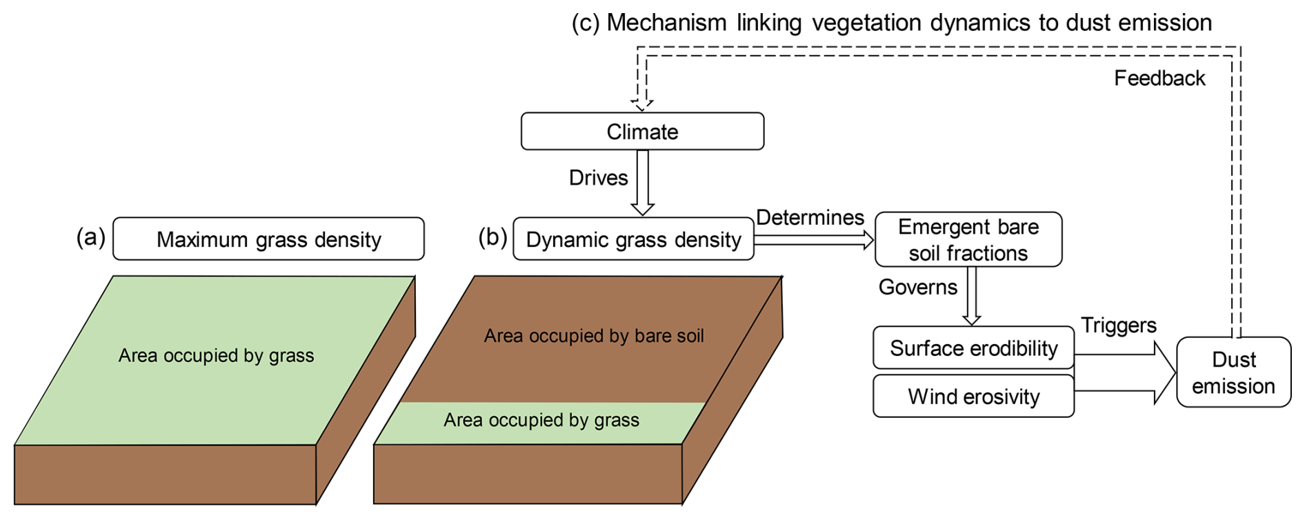
Figure 1 Conceptual framework of grassland density under varying resource availability and its link to dust emission. With high resource availability, grassland density is able to reach the maximum density (a), while low resource availability dynamically results in lower grassland density (b). The conceptual framework (c) illustrates the mechanism linking vegetation dynamics to dust emission. The schematic shows how climatic drivers control dynamic grassland density, which in turn determines the bare soil fraction and surface erodibility. Dust emission is triggered when the surface is exposed to sufficient wind erosivity, creating a potential feedback loop with the climate system.

Grassland dynamics can be expressed as the variation of “grassland density” or “plant cover”. The term “density” in an ecosystem can have multiple definitions, including population density, measured as the number of individuals per area (Zhu et al., 2015), or mass density, expressed as mass per unit area (Rietkerk et al., 2002). In this study, we focus on population density, defined as the number of individuals per unit area. Here, each individual represents a conceptual unit that occupies 1 m² of land, rather than a physical plant. Accordingly, the unit of grassland density in this study is expressed as m² m⁻². For instance, a hectare of grassland with a density of 1 contains 10 000 individuals, occupying a total area of 10 000 m² ha⁻¹ (Fig. 1a). A density of 0.25 therefore corresponds to 2500 individuals occupying 2500 m² ha⁻¹ (Fig. 1b). In this framework, grassland density thus relates to the geometrically fractional occupancy of conceptual individuals, and differs from “plant cover” which refers to the optically projected vegetation coverage in grasslands. Although regional estimates are available (Booth et al., 2005; Dusseux et al., 2014; John et al., 2018; Melville et al., 2019; Diatta et al., 2023), spatially explicit global estimates of grassland density remain challenging, due to inconsistent definitions of grassland density (Rietkerk et al., 2002) and the inherent difficulties of direct measurement (Vogel and Masters, 2001; Hamada et al., 2021). Global spatially explicit fractional vegetation cover data, on the other hand, has been estimated through remote sensing FCOVER product from Copernicus Land Monitoring Service (Copernicus Land Monitoring Service, 2020).

In this study, we use the land surface model ORCHIDEE (trunk version, r9010), which is part of the IPSL-CM Earth System Model (Boucher et al., 2020). Currently, ORCHIDEE prescribes a globally fixed grassland density by default, implying that all the global grasslands are stocked with the maximum possible number of conceptual individuals. Consequently, the model simulates frequent mortality events driven by this density limit, particularly in (semi-)arid grid cells. In addition, a fixed density does not respond to resource availability, which hinders the study of dust emission responses in the presence of grassland when the land surface model is coupled to an atmospheric model (Boucher et al., 2020). Finally, the fixed density makes an evaluation of the model using observed or remotely sensed vegetation density and plant cover meaningless.

To address the limitations of the fixed grassland density in ORCHIDEE, we revised the model to simulate a dynamic grassland density, with the aims of: (a) simulating the response of the bare soil fraction in grasslands to environmental changes, providing a foundation for predicting the long-term spatiotemporal dynamics of dust emissions in future work; (b) enhancing grassland survival, particularly in (semi-)arid regions; and (c) better representing the grassland leaf area index (LAI), which is a key variable in simulating land–atmosphere processes such as photosynthesis, transpiration, albedo and the energy budget. To these aims, we replaced the fixed density approach with a physiology-based approach to simulate grassland density in ORCHIDEE, and ran simulations with both approaches to: (1) evaluate our simulated grassland density against regional field-based data; (2) compare the simulated fractional vegetation cover (FVC) with satellite-based dataset; (3) assess whether dominant grassland types are consistent with their relative contributions to grassland density, and analyse the emergent relationship between precipitation and grassland density; (4) compare the frequency of mortality events between the fixed and dynamic approach for grassland density; (5) quantify the responses of mortality events in grasslands to aridity; and (6) evaluate the simulated leaf area index (LAI) against remotely sensed observations.

2 Methods

2.1 The land surface model ORCHIDEE

ORCHIDEE is a process-based land surface model capable of simulating the carbon, nitrogen, water, and energy cycles, including vegetation dynamics, biogeochemical fluxes, and plant competition (Krinner et al., 2005; Naudts et al., 2015; Vuichard et al., 2019). In ORCHIDEE trunk version r9010, each grid cell may contain up to 15 plant functional types (PFTs), representing eight different types of forests, four types of grasslands, two types of croplands, and bare soil (defined as a separate PFT). Each PFT has a value for its fraction (V_fra), and the sum of V_fra from all 15 PFTs is equal to 1 within each grid cell. The value of V_fra is derived from a land cover map that is in turn obtained from post-processing of remote sensing observations (Poulter et al., 2015; ESA, 2017).

ORCHIDEE distinguishes four grassland types: temperate C₃ grassland, tropical C₃ grassland, boreal C₃  rassland, and C₄ grassland. C₃ and C₄ plants use the C₃ or C₄ photosynthesis pathways, respectively (Taylor et al., 2010). In light of this study's emphasis on (semi-)arid grasslands, boreal C₃ grassland was excluded from the analysis. For each PFT, ORCHIDEE simulates processes such as photosynthesis, phenology, carbon and nitrogen allocation, senescence, turnover, and mortality, based on PFT-specific parameter sets.

2.2 Grassland density

2.2.1 Fixed density approach

The grassland density in ORCHIDEE is calculated as:

$$\begin{array}{}\text{(1)}& D=N_{\max }\end{array}$$

where D refers to grassland density, defined as the fractional area occupied by conceptual individuals (m² m⁻²). By default, the number of conceptual individuals (N_max) in grassland is set to be 10 000 per hectare, with each occupying 1 m² of land. Consequently, the default vegetation density for grasslands in the model is fixed at 1 m² m⁻².

2.2.2 Dynamic density approach

A grassland with the abundant resources (i.e., water, light, nitrogen, temperature, and CO₂) is able to support high grassland density (Fig. 1a) with high biomasses per conceptual individual. In contrast, for grasslands with limited resources, both the density and the individual biomass might be low (Fig. 1b). In the fixed density approach, for grasslands with limited resources, the available resources per conceptual individual might be too limited to sustain sufficient reserve and labile carbon, thereby limiting vegetation growth. In the model, the carbon and nitrogen biomass of a conceptual individual are distributed among different pools (Fig. 2), including leaf (C_leaf), stem (C_stem), root (C_root), fruit (C_fruit), reserve (C_reserve), and labile (C_labile). Carbon and nitrogen in the leaf, stem, root, and fruit pools are allocated to specific structural components, whereas carbon and nitrogen in the reserve and labile pools are non-structural and can be found throughout the plant. Reserve carbon and nitrogen refer to a more stable pool, whereas labile carbon and nitrogen represent a rapidly mobilized pool (Gupta and Kaur, 2000). Reserve and labile carbon and nitrogen are considered primary sources for immediate regrowth following defoliation or the alleviation of stress (Volaire, 1995). In this study, we considered the sum of reserve and labile carbon for subsequent calculations.

The dynamic density approach simulates grassland density by adjusting the population to the maximum number of conceptual individuals that can be sustained by the available resources (Fig. 2). This adjustment is performed on a daily basis, primarily in response to the total reserve and labile carbon levels.

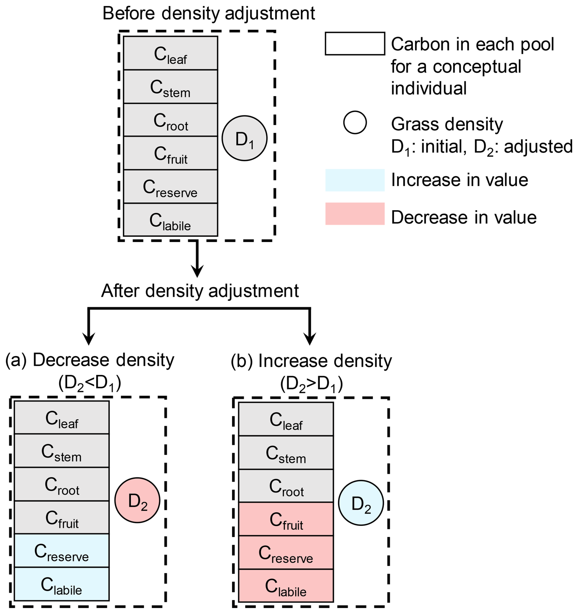
Figure 2 Schematic of the carbon (C) redistribution mechanism during density adjustments. The model simulates the transition from an initial state with density D₁ (top panel) to two possible scenarios after adjustment to density D₂ (bottom panels): a decrease in density (a) or an increase in density (b). Blue indicates an increase and red indicates a decrease in values for both carbon pools (rectangles) and grassland density (circles).

When the reserve and labile carbon in the plant drop below their respective target values and this condition persists over a longer time period, a mortality risk ensues (Volaire, 1995). The dynamic density approach in ORCHIDEE accounts for this case by decreasing the number of conceptual individuals when the total reserve and labile carbon falls below a simulated target value. Therefore, the labile and reserve carbon are redistributed among the fewer conceptual individuals (Fig. 2a), whose chances for future survival have increased. The carbon in other compartments (leaf, stem, root and fruit) in each conceptual individual remains constant when the number of conceptual individuals is decreased (Fig. 2a). The nitrogen content of each compartment in a conceptual individual is updated by multiplying the previous nitrogen content by the ratio of the previous density to the current density. A minimum density of 0.05 is set to avoid numerical errors in the model.

The ORCHIDEE model distinguishes eight phenological stages (P_S): (1) Planting: emergence of new plant, (2) Buds: appearance of buds, (3) Leaf: onset of leaf, (4) Growth: presence of canopy, (5) Pre-senescence: cessation of vegetation growth, (6) Senescence: senescence of plant, (7) Dormancy: dormancy of plant and (8) Death: death of plant. It has been reported previously (e.g. Volaire, 1995; Sarath et al., 2014; Keep et al., 2021) that during vegetation senescence, the reserve or labile carbon experiences a peak influx of carbon reallocated from leaves, and during dormancy, reserves are conserved for the upcoming growing season. Therefore, grassland density is only decreased during the following phenological stages: pre-senescence, senescence, and dormancy, when the reserve and labile carbon should attain their annual peak. A decrease in grassland density in one timestep of the model is calculated as follows:

$$\begin{array}{}\text{(2)}& \left\{\begin{array}{l}{C}_{\mathrm{all}}\times D_{\mathrm{1}}=\left(C_{\mathrm{all}}-C_{\mathrm{res},\mathrm{1}}-C_{\mathrm{lab},\mathrm{1}}\right)\times D_{\mathrm{2}}+T_{\mathrm{res}}+T_{\mathrm{lab}}\\ D_{\mathrm{2}}=\frac{\left(C_{\mathrm{all}}\times D_{\mathrm{1}}-T_{\mathrm{res}}-T_{\mathrm{lab}}\right)}{\left(C_{\mathrm{all}}-C_{\mathrm{res},\mathrm{1}}-C_{\mathrm{lab},\mathrm{1}}\right)}\end{array}\right.\end{array}$$

where C_all, C_res, and C_lab are the carbon biomasses of all compartments, the reserve, and the labile pool of a conceptual individual, respectively, with units of grams of carbon per individual (g C per individual); the indices 1 and 2 refer to the value before and after the density adjustment; T_res and T_lab are the targets for reserve carbon and labile carbon in the PFT (g C m⁻²), respectively, which are calculated in ORCHIDEE as:

$$\begin{array}{}\text{(3)}& {\displaystyle }\begin{array}{rl}{T}_{\mathrm{res}}=& \min \left[\mathit{\beta }\times \left(B_{\mathrm{root}}+B_{\mathrm{stem},\mathrm{above}}+B_{\mathrm{stem},\mathrm{below}}\right),\right.\\ & \left.{\displaystyle \frac{\exp (\mathrm{LAI}\times k)-\mathrm{1}}{k\times {\mathrm{SLA}}_{\mathrm{init}}}}\times \left(\mathrm{1}+{\displaystyle \frac{\mathit{\delta }}{\mathit{\lambda }}}\right)\right]\end{array}\text{(4)}& {\displaystyle }\begin{array}{rl}{T}_{\mathrm{lab}}=& \max \left[t\times \mathit{\gamma }\times \left(N_{\mathrm{leaf}}+N_{\mathrm{root}}+N_{\mathrm{fruit}}+N_{\mathrm{stem},\mathrm{above}}\right.\right.,\\ & \left.+N_{\mathrm{stem},\mathrm{below}}\right)\left.,\mathrm{10}\times {\mathrm{GPP}}_{\mathrm{week}}\right]\end{array}\end{array}$$

where β is the fraction of stem mass stored in the reserve pool during the growing season (unitless); B_root, B_stem,above, and B_stem,below are the carbon biomasses of the root, aboveground stem, and belowground stem, respectively, for a given PFT (g C m⁻²); k is the extinction coefficient of the leaf nitrogen content profile within the canopy (unitless); SLA_init is the initial specific leaf area at the bottom of the canopy (m² g⁻¹ C); δ is the fraction of maximum root biomass covered by reserve biomass (unitless); λ is a scaling factor converting stem mass into root mass (unitless); t is the turnover coefficient of the labile carbon pool (unitless); γ is the parameter used to calculate the labile pool (unitless); N_leaf, N_root, N_fruit, N_stem,above and N_stem,below are the nitrogen biomasses of the leaf, root, fruit, aboveground stem, and belowground stem in the PFT, respectively (g N m⁻²); and GPP_week is the weekly gross primary productivity (g C m⁻² d⁻¹).

When the carbon content in both reserve and labile pools exceeds their respective targets, and carbon is present in the fruit pool, the excessive carbon from the fruit, reserve, and labile pools will be used to create new conceptual individuals. After updating the number of conceptual individuals, the carbon in labile and reserve pools is reset to their target values, and the carbon in fruit pool becomes zero (Fig. 2b). The density is only increased during the phenological stage labelled as “Growth”. This approach for increasing grassland density reflects asexual recruitment of perennial plants (Blair et al., 2013), which is implemented in the model using conceptual units rather than actual plants. The carbon in other compartments (leaf, stem and root) in each conceptual individual remains constant. Nitrogen is treated using the same method as that applied to decreasing density. An increase in grassland density is calculated as follows:

$$\begin{array}{}\text{(5)}& \left\{\begin{array}{l}{C}_{\mathrm{all}}\times D_{\mathrm{1}}=\left(C_{\mathrm{all}}-C_{\mathrm{res},\mathrm{1}}-C_{\mathrm{lab},\mathrm{1}}-C_{\mathrm{fruit},\mathrm{1}}\right)\times D_{\mathrm{2}}+T_{\mathrm{res}}+T_{\mathrm{lab}}\\ D_{\mathrm{2}}=\frac{\left(C_{\mathrm{all}}\times D_{\mathrm{1}}-T_{\mathrm{res}}-T_{\mathrm{lab}}\right)}{\left(C_{\mathrm{all}}-C_{\mathrm{res},\mathrm{1}}-C_{\mathrm{lab},\mathrm{1}}-C_{\mathrm{fruit},\mathrm{1}}\right)}\end{array}\right.\end{array}$$

where C_fruit,1 refers to the carbon biomass from the fruit pool at the conceptual individual level before density adjustment (g C per individual).

2.3 Model evaluation against regional field observations and global dataset

Two independent datasets were used for model evaluation. First, we compared the simulated grassland density directly against regional field-based observations. Second, we compared the fractional vegetation cover (FVC) – derived from the simulated grassland density in ORCHIDEE – against a global satellite-based dataset.

In order to directly assess the ecological realism of the simulated grassland density, we compared model outputs with field-based estimates from five published regional case studies. These studies span a range of grassland ecosystems: a temperate European grassland in France (Dusseux et al., 2014), the Eurasian steppe on the Mongolian Plateau (John et al., 2018), a meadow in the USA (Booth et al., 2005), a Sahelian rangeland in Senegal (Diatta et al., 2023), and a grass-shrub community in Australia (Melville et al., 2019), as listed in Table 1.

Table 1 Evaluation of simulated grassland density from ORCHIDEE against field-based estimates from various grassland sites (all values in m² m⁻²).

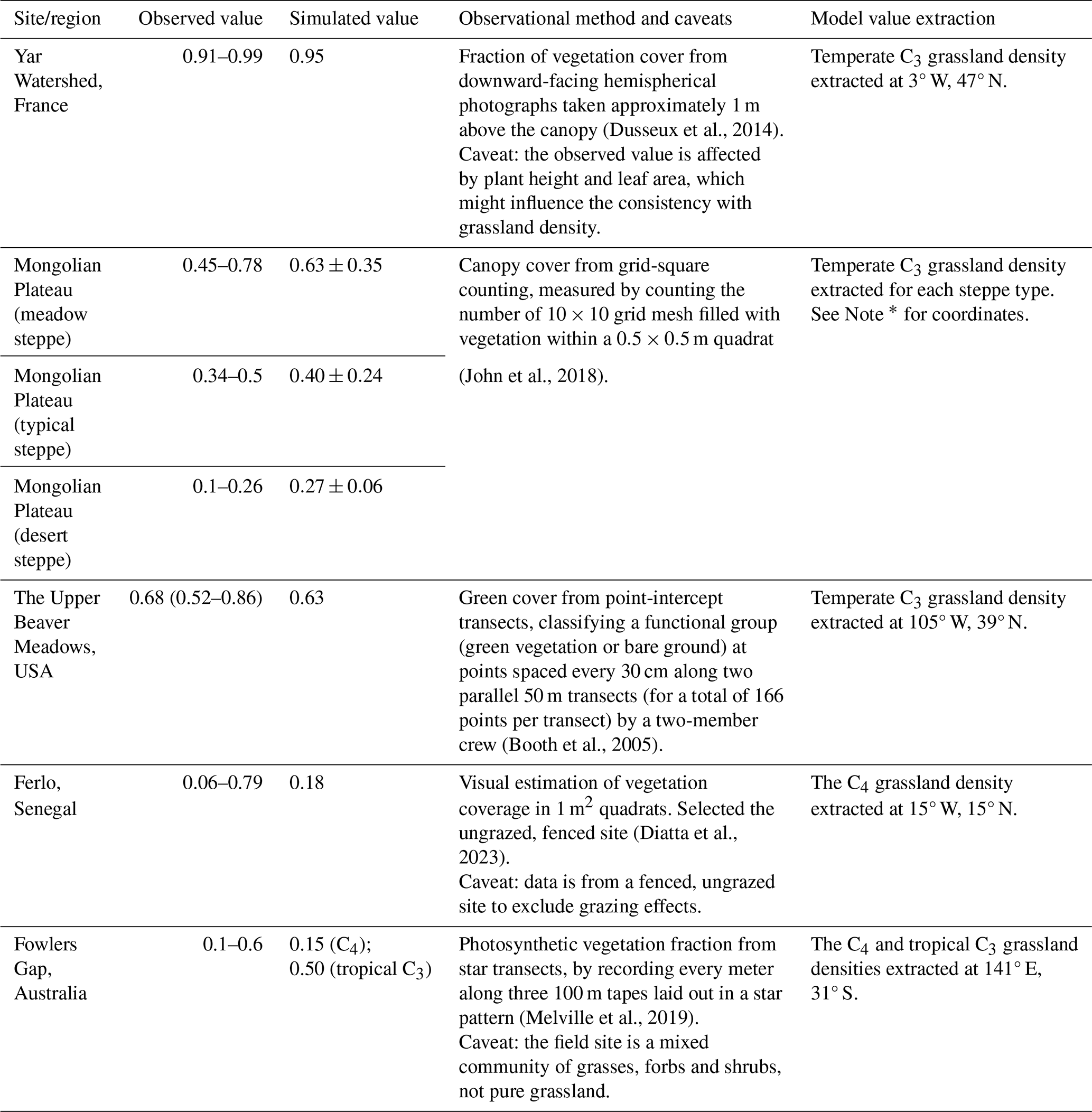
^* Note: according to Fig. 1 in John et al. (2018), we delineated three types of steppe on the Mongolian Plateau in ORCHIDEE: 97–103° E, 45–47° N in the meadow steppe, excluding other steppe types within this rectangle; 111–117° E, 39–47° N in the typical steppe, excluding forest meadow and meadow steppe within this range; 89–111° E, 39–45° N in the desert steppe, excluding desert and typical steppe areas.

We acknowledge that the metrics from field-based observation are not identical to the grassland density defined in our study. However, the five case studies provide metrics that are thought to be sufficiently similar to be compared to the metric in ORCHIDEE, i.e., the fractional area occupied by conceptual individuals (Fig. 1a and b). The case-studies provide the area-based geometric estimates – either by counting points classified as vegetation within quadrats (John et al., 2018; Diatta et al., 2023), along transects (Booth et al., 2005; Melville et al., 2019), or from downward-facing hemispherical photographs to estimate green vegetation cover (Dusseux et al., 2014). Detailed descriptions of each dataset, including observed and corresponding simulated values, measurement methods, and caveats of the selected methods, are provided in Table 1. The hemispherical photography method may be influenced by plant height and leaf area (Dusseux et al., 2014); the effects of grazing were controlled by selecting fenced sites (Diatta et al., 2023); and the observational sites included not only grasses but also forbs and shrubs, although grasses were dominant (Melville et al., 2019).

Furthermore, the simulated fractional vegetation cover was compared against the Copernicus Land Monitoring Service FCOVER product (Copernicus Land Monitoring Service, 2020). We selected the year 2004 for this comparison, as it matches the static global land cover map used throughout this study. The FCOVER product (originally at ∼0.003° resolution) was regridded to our model's 2°×2° resolution using RemapCon (Jones, 1998; Goudiaby et al., 2024) in the Climate Data Operators library for Linux. To ensure a fair comparison, we calculated the corresponding fractional vegetation cover (FVC) specifically from the targeted grassland PFTs within ORCHIDEE using the equation:

$$\begin{array}{}\text{(6)}& \begin{array}{rl}\mathrm{FVC}& =D_{\mathrm{temp}{\mathrm{C}}_{\mathrm{3}}}\times V_{\mathrm{fra},\mathrm{temp}{\mathrm{C}}_{\mathrm{3}}}+D_{{\mathrm{C}}_{\mathrm{4}}}\times V_{\mathrm{fra},{\mathrm{C}}_{\mathrm{4}}}\\ & +D_{\mathrm{trop}{\mathrm{C}}_{\mathrm{3}}}\times V_{\mathrm{fra},\mathrm{trop}{\mathrm{C}}_{\mathrm{3}}}\end{array}\end{array}$$

where $D_{\mathrm{temp}{\mathrm{C}}_{\mathrm{3}}}$, $D_{{\mathrm{C}}_{\mathrm{4}}}$, and $D_{\mathrm{trop}{\mathrm{C}}_{\mathrm{3}}}$ are the simulated grassland density (1.0 for the fixed density approach, 0.05–1.0 for our new dynamic density approach) and $V_{\mathrm{fra},\mathrm{temp}{\mathrm{C}}_{\mathrm{3}}}$, $V_{\mathrm{fra},{\mathrm{C}}_{\mathrm{4}}}$, and $V_{\mathrm{fra},\mathrm{trop}{\mathrm{C}}_{\mathrm{3}}}$ are the fractional area of each grassland PFT (temperate C₃, C₄, tropical C₃) within one grid cell.

Given that this study aims to improve grassland density simulation, the comparison of FVC focused specifically on grasslands. To isolate the target ecosystems where grasslands dominate and exclude the canopy cover from other vegetation as much as possible, we applied a (semi-)arid region mask based on the aridity index map by Zomer et al. (2022).

2.4 Determination of PFT dominance and co-existence

We used the fraction of vegetation type (V_fra), defined as the ratio of the area covered by a given PFT to the total area of the grid cell, as the basis for classification. In this study, we defined a grassland PFT as “dominant” in a given grid cell if two conditions were simultaneously met: (1) its V_fra was 0.5 or higher, and (2) the V_fra of other grassland PFTs was lower than 0.1. When two or more grassland PFTs had V_fra values above 0.1, they were considered to co-exist.

2.5 Mortality events in grasslands

In reality, under very arid conditions, plants may be unable to grow during unfavourable years (Blair et al., 2013; Bodner and Robles, 2017). However, seed banks or rhizomes in the soil can enable regrowth when environmental conditions become favourable again (Blair et al., 2013). In ORCHIDEE, transferring carbon from reserve to leaves initiates the growing season for deciduous vegetation, but it does not account for a long-term reserve pool that can retain reserves over several years. Under unfavourable conditions, the reserves will deplete, preventing vegetation from re-growing in the following years. In ORCHIDEE, this can be monitored through phenological stage, which is set to one of the eight stages of the plant (see above).

When, at the end of the growing season, the reserve and labile carbon pools are empty, the grassland is considered dead in ORCHIDEE, and its phenological stage is set to “Death”. At the start of the next growing season, a new grassland is planted by the model, and its phenological stage is updated to “Planting”. The initial biomass from the planted grassland is taken directly from the atmosphere, thus bypassing germination and the early stages of plant development. The transition of the phenological stages from “Death” to “Planting” is recorded and counted as a single mortality event. If the environmental conditions become favourable again, the grassland will continue to grow. If not, it will die again. Therefore, the vegetation in each grid cell might experience repeated mortality events over decades, as it is replanted following each mortality event (Fig. S1 in the Supplement).

As long as these mortality events remain infrequent, they have little impact on the simulated fluxes because the cumulated photosynthesis by far exceeds the carbon used to initialize the grassland biomass. If, however, the mortality and replanting cycles become frequent, the repetitive addition of the initial carbon may become substantial compared to carbon assimilation through photosynthesis. For example, in tropical C₃ grassland at grid cell (59° E, 39° N) using the fixed density approach, frequent mortality events resulted in unrealistic productivity patterns, characterized by abrupt post-mortality spikes resulting from the addition of the initial biomass when replanting (Fig. S1).

Grasslands are modelled as perennial vegetation in ORCHIDEE; hence, a skilful model is expected to simulate infrequent mortality events in grasslands, reflecting the inherent resilience and stability of grassland ecosystems. We defined a threshold for such “infrequent mortality” as fewer than five times over a 51-year simulation period. This benchmark was supported by ecological records of prolonged droughts, such as the 1930s Dust Bowl in the Great Plains (Blair et al., 2013) and a decade-long drought in southern Arizona (Bodner and Robles, 2017). The events caused widespread mortality in perennial grasslands, implying that mortality on a decadal scale (i.e., approximately once per decade) is realistic under extreme conditions. Consequently, exceeding such a frequency might indicate unrealistic model behaviour. Therefore, reducing the number of mortality events is considered an indication of model improvement for the representation of grasslands.

To quantify the impact of PFT mapping errors on simulated grassland mortality, we first identified all grassland grid cells where mortality events occurred in the simulation using the dynamic density approach (Fig. S2). Next, a set of criteria was established to identify “constrained regions” where the persistence of grassland vegetation is considered unlikely. A grid cell was classified as constrained if it met at least one of the following three conditions: (1) location within a hyper-arid zone: In these zones, little vegetation can survive, and vascular plants are often restricted to ephemeral streams receiving runoff (Huang et al., 2016; Groner et al., 2023). (2) Critically low LAI: the observed LAI for viable grasslands is typically greater than 0.1 (Si et al., 2012; Haynes et al., 2019), which suggests regions with mean annual LAI < 0.1 are unsuitable for growth. (3) Risk of ecosystem breakdown: Calculated aridity (Eq. 8) greater than 0.83 is associated with ecosystem breakdown (Berdugo et al., 2020). Finally, we quantified the proportion of grid cells with simulated mortality (for all grass PFTs) that occurred in these constrained regions.

2.6 Leaf area index (LAI) for grasslands

Remote sensing-based LAI observations (Myneni et al., 2021; Wan et al., 2024) were used to evaluate model output of LAI for grasslands. We utilized two observational (satellite-based) datasets: MODIS LAI (2004–2020), originally at a resolution of 1 km with a 4 d temporal frequency (Myneni et al., 2021), and Sentinel-2 data for 2019 at a spatial resolution of 10 m (Wan et al., 2024). In order to compare them with the 2°×2° global simulations in ORCHIDEE, both datasets were aggregated to the spatial resolution of the simulations. In both cases, LAI values were filtered based on land cover classification, to retain only grassland pixels. For MODIS, the grassland classification was based on MCD12Q1 land cover product (Myneni et al., 2021). The resulting grassland grid cells were then spatially regridded using a first-order conservative remapping for grid cells classified as grassland, which preserves the total integrated quantity during spatial interpolation, implemented via RemapCon (Jones, 1998; Goudiaby et al., 2024) in the Climate Data Operators library (CDO) for Linux. For Sentinel-2, grassland pixels were identified using the GLC_FCS30D land cover dataset (Zhang et al., 2024). The LAI values were aggregated by computing the arithmetic mean of all high-resolution pixels classified as grassland (code 130) within each 2°×2° grid cell, using Python scripts.

Leaf area index is a central variable in climate models as it is one of the functional links between the land surface and the atmosphere. Thus, a skilful land surface model is expected to simulate realistic spatial and temporal patterns in LAI. LAI is the product of leaf carbon mass and specific leaf area (SLA). In ORCHIDEE, SLA varies vertically through the canopy. To account for this vertical variation, LAI is calculated using a dynamic SLA formulation, as expressed in Eq. (7), where the extinction coefficient k represents the vertical profile of leaf nitrogen content within the canopy. This calculation is performed at the PFT level as follows:

$$\begin{array}{}\text{(7)}& \mathrm{LAI}={\displaystyle \frac{\log \left(\mathrm{1}+k\times B_{\mathrm{leaf}}\times {\mathrm{SLA}}_{\mathrm{init}}\right)}{k}}\end{array}$$

where B_leaf refers to the leaf biomass (g C m⁻²) calculated as the product of individual leaf biomass (g C per individual) and grassland density.

The land cover map used in ORCHIDEE was derived from the ESA CCI Land Cover dataset (ESA, 2017) and converted into PFT fractional maps using a cross-walking table (Poulter et al., 2015). However, neither observational dataset distinguishes specific types of grasslands. To enable comparison, all grassland PFTs in ORCHIDEE were merged into a single grassland category by computing the weighted average LAI across PFTs, using the fraction of vegetation type (V_fra) for each grassland PFT as the weighting factor. Only grid cells where the total V_fra of grassland PFTs exceeded 0.1 in ORCHIDEE were included for the LAI analysis.

2.7 Aridity

Aridity (A) serves as an important indicator of water scarcity (Berdugo et al., 2020), and is calculated as:

$$\begin{array}{}\text{(8)}& A=\mathrm{1}-{\displaystyle \frac{P}{E_{\mathrm{PET}}}}\end{array}$$

where P is precipitation, taken from input forcing data, and E_PET refers to potential evapotranspiration simulated in ORCHIDEE. A high aridity value, e.g., 0.5 or more, indicates that the region is limited in water resources.

2.8 Tuning of C₄ grassland parameters

Field observations indicate that C₄ grasslands are generally more drought-tolerant than C₃ grasslands (Taylor et al., 2010). However, in ORCHIDEE, the simulated density of C₄ grasslands was too high under strong water limitations (Figs. S3, S4a and S5c). This suggested that the model underestimated the sensitivity of C₄ grasslands to water stress, leading to an overestimation of grassland density in these areas. This issue was addressed by recalibrating PFT-specific parameters for C₄ grasslands, related to the targets for reserve and labile carbon (see below) and the water stress function (see below). The adjustments were tested in southern Africa for C₄ grasslands, and the recalibrated parameters were retained as they improved the correlation between precipitation and grassland density (Fig. S4).

The first parameter that was recalibrated controls the target level for reserve and labile carbon, which is a critical driver of grassland density in the dynamic density approach. The adjustment consisted of applying a scaling factor to the target for reserve and labile carbon. A value of 1 (Fig. S5c) indicates that targets remain at the default state, whereas values of 0.5 and 0.75 (Fig. S5a and b) represent lower carbon targets, and values of 1.25 and 1.5 (Fig. S5d and e) represent higher carbon targets, corresponding to less and more stringent growth requirements, respectively.

As shown in Fig. S5f, this analysis revealed that the average density (diamonds) over this region remained high (greater than 0.9) and relatively insensitive across most factors, with only a slight drop for a scaling factor of 1.5. In contrast, the spatial variability (represented by the 5th–95th percentile range) was more sensitive to the scaling factor. This range was narrow for factors of 0.5 and 0.75 but widened significantly for values greater than 1. This widening, particularly at 1.5, was driven by a significant drop in the 5th percentile, indicating much greater spatial heterogeneity because a larger portion of grid cells was experiencing lower density (as also seen in Fig. S5e). Although a scaling factor of 1.5 slightly decreased the regional mean, it introduced a spatial variability that better reflected real-world heterogeneity. Therefore, a value of 1.5 was applied to increase the target level for reserve and labile carbon in C₄ grasslands.

The second parameter controls the water stress for transpiration, which ranges from 1 (no stress) to 0 (severe stress). By default, the function of water stress (W_stress) for transpiration is formulated as follows:

$$\begin{array}{}\text{(9)}& W_{\mathrm{stress}}=\min \left(\mathrm{1},\max \left(\mathrm{0},{\displaystyle \frac{\mathit{\theta }-{\mathit{\theta }}_{\mathrm{wilt}}}{{\mathit{\theta }}_{\mathrm{nostress}}-{\mathit{\theta }}_{\mathrm{wilt}}}}\right)\right)\times R_{\mathrm{profile}}\end{array}$$

where θ refers to soil moisture (kg m⁻²), θ_wilt refers to soil moisture at the wilting point (kg m⁻²), θ_nostress is the soil moisture when there is no water stress (kg m⁻²), and R_profile is the normalized root mass or length fraction (unitless).

This water stress function can be switched to an exponential formulation with a parameter α, written as below:

$$\begin{array}{}\text{(10)}& \begin{array}{rl}{W}_{\mathrm{stress}}& =\min \left(\mathrm{1},\exp \left[-\mathit{\alpha }\times \left({\displaystyle \frac{{\mathit{\theta }}_{\mathrm{fc}}-{\mathit{\theta }}_{\mathrm{wilt}}}{{\mathit{\theta }}_{\mathrm{nostress}}-{\mathit{\theta }}_{\mathrm{wilt}}}}\right)\right.\right.\\ & \left.\left.\times \left({\displaystyle \frac{{\mathit{\theta }}_{\mathrm{nostress}}-\mathit{\theta }}{\mathit{\theta }-{\mathit{\theta }}_{\mathrm{wilt}}}}\right)\right]\right)\times R_{\mathrm{profile}}\end{array}\end{array}$$

where θ_fc refers to soil moisture at field capacity (kg m⁻²), and the value for parameter α can range from 0 to 10, with higher values indicating the plant is more limited by water stress (Raoult et al., 2021). In this study, values of α=1, 2, 4, and 8 were tested for southern Africa (Fig. S6).

As shown in Fig. S6f, the model was relatively insensitive to the choice between the linear formulation and exponential formulations for low α values (e.g., α=1, 2). In these cases, both the mean density and the 5th–95th percentile range remained high and stable, indicating uniformly high grassland density. The impact became pronounced at higher α values. At α=4, the percentile range began to widen (driven by a drop in the 5th percentile), indicating an increase in spatial heterogeneity. This effect was strongest at α=8, where both the mean density and the 5th percentile dropped significantly. This latter setting resulted in the widest variability range, reflecting the much lower densities seen in the corresponding spatial map (Fig. S6e). Therefore, α=8 was selected for the global simulations to enhance water stress sensitivity of C₄ grasslands.

2.9 Simulations

All simulation experiments started with a 200-year spin-up at a spatial resolution of 2°×2° at a global scale while cycling over the CRU-JRA climate forcing from 2004 to 2020 (Harris et al., 2020), which aligns with the period of MODIS LAI observations. In these simulations, the CO₂ concentration was set to 350 ppm globally, and the land cover map was for the year 2004, derived from ESA CCI Land Cover dataset (Poulter et al., 2015; ESA, 2017). The year 2004 was chosen as it corresponds to the starting year of the MODIS data for LAI used in this study. Land cover change was not accounted for and the fixed density approach was used for the spin-up. During the spin-up, the soils are brought to equilibrium every 15 years with the 15-year average litter inputs. The nitrogen cycle in the ORCHIDEE model requires that the semi-analytical spin-up is repeated about 10 times before an equilibrium is reached (Vuichard et al., 2019). After 150 years of simulation, we checked that the soil passive carbon pools had reached an equilibrium, with the values fluctuating within a 20 % range over the remaining 51 simulation years (Lardy et al., 2011). Once the soil carbon and nitrogen pools were in equilibrium, the simulation experiment branched off with two configurations using the fixed density approach (Sect. 2.2.1), and the dynamic density approach (Sect. 2.2.2).

The simulation results from the two configurations were analysed by comparing the grassland density, mortality, the response of mortality in grassland to aridity, and the mean annual grassland LAI. To align with the 17-year period (2004–2020) of the CRU-JRA forcing data, we present the averaged values for grassland density and mean annual LAI over the same period. The mortality events were accumulated and analysed over 51 simulation years taken after the model had reached equilibrium following the initial 150 years of the spin-up.

3 Results

3.1 Spatial distribution of simulated grassland density

With the dynamic density approach, the globally simulated grassland density varied between the minimum and maximum threshold values of 0.05 and 1, respectively (Fig. 3). Throughout the 17-year period (2004–2020), 56 % of the grid cells in temperate C₃ grasslands, 66 % in the C₄ grasslands, and 33 % in the tropical C₃ grasslands maintained the maximum density (Fig. 3a–c). In contrast, grassland density reached the minimum value in fewer than 1 % of the grid cells across all three grassland types. The majority of grassland grid cells had a density ranging between 0.9 and 1, i.e., 75 % of temperate C₃ grasslands, 79 % of C₄ grasslands, and 59 % of tropical C₃ grasslands (Fig. 3d–f).

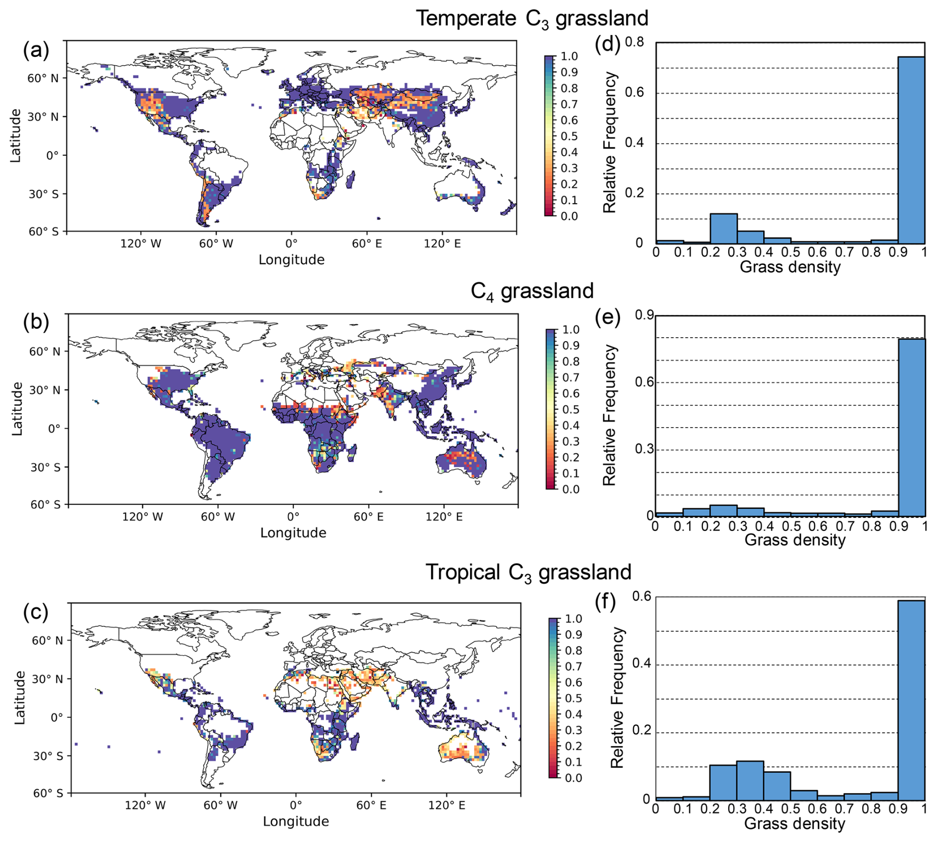
Figure 3 Global distribution (a–c) and frequency histograms (d–f) of simulated grassland density for three grassland types. Global maps show the 17-year average (2004–2020) grassland density simulated with the dynamic density approach for (a) temperate C₃, (b) C₄, and (c) tropical C₃ grasslands. The corresponding histograms (d–f) show the relative frequency of simulated density values for each grassland type.

Temperate C₃ grasslands in eastern USA, Europe, eastern China, and New Zealand were simulated at the maximum density, in contrast to areas such as western USA, Middle East and northern China where ORCHIDEE simulated lower densities. The C₄ grasslands were simulated at a lower than maximum density in India, Sahel, southern Africa and middle Australia. By contrast, in tropical C₃ grasslands, densities between the minimum and the maximum were simulated in regions such as the Middle East, northern Africa, southern Australia, and southern Africa, whereas the maximum density was simulated in South America and southern east Asia.

3.2 Evaluation of simulated grassland density

The simulated grassland density was compared against direct field-based estimates for five regional case studies (Table 1). Over temperate grassland in France, the simulated density of 0.95 was within the observed range of 0.91 to 0.99 (Dusseux et al., 2014). This consistency extended to the Upper Beaver Meadows site in North America, with a simulated density of 0.63 that approached the observed mean of 0.68 (Booth et al., 2005). For the desert steppe (with the cold desert climate) of the Mongolian Plateau, the simulated value of 0.27 was just outside the observed range of 0.10–0.26 (John et al., 2018). Furthermore, simulated average densities for typical steppes characterized by the semi-arid climate (0.40) and meadow steppes characterized by the subarctic climate (0.63) fell within their respective observed ranges of 0.34–0.50 and 0.45–0.78 (John et al., 2018). In the Sahelian fenced rangeland of Senegal, the simulated density of 0.18 was in the low range of the large observed range of 0.06 to 0.79. Finally, for the mixed grass-shrub community in Australia, both the simulated C₄ (0.15) and tropical C₃ (0.50) grass densities were consistent with the field-based range of 0.1 to 0.6 (Melville et al., 2019).

The dynamic density approach was further evaluated against a comparison of FVC with a global satellite-based FCOVER product (Copernicus Land Monitoring Service, 2020) (Fig. S7). The spatial correlation (Pearson's r) between the model and the FCOVER data increased from r=0.11 with the fixed density approach to r=0.24 with the dynamic density approach. The dynamic density approach also exhibited a lower RMSE (0.22) compared to the fixed density approach (0.26). This improvement was particularly evident in western United States, Asia, southern Africa, and Australia, where the dynamic scheme simulated a lower and more realistic FVC (Fig. S7c), in better agreement with the FCOVER dataset, compared to the fixed density approach (Fig. S7b). Such regional-scale improvement is consistent with the findings from the regional field-based comparisons.

As a reminder for the following results, the land cover map represents the fractional area covered by each PFT (V_fra) within one grid cell, whereas grassland density reflects the fractional area occupied by conceptual individuals within the grassland PFT. A high V_fra for a given PFT indicates that the PFT is the dominant vegetation type in that area, but it does not necessarily mean that the PFT has a high vegetation density. However, under natural and undisturbed conditions, our expectation is that when a PFT is dominant (explained in Sect. 2.4), its vegetation density should be higher than that of other PFTs with lower V_fra. Conversely, when multiple PFTs coexist (Sect. 2.4), their densities should be similar. Therefore, we calculated the relative contribution of each of the three grassland types to the total grassland density (Fig. 4b), allowing us to focus on their proportional importance rather than their absolute values.

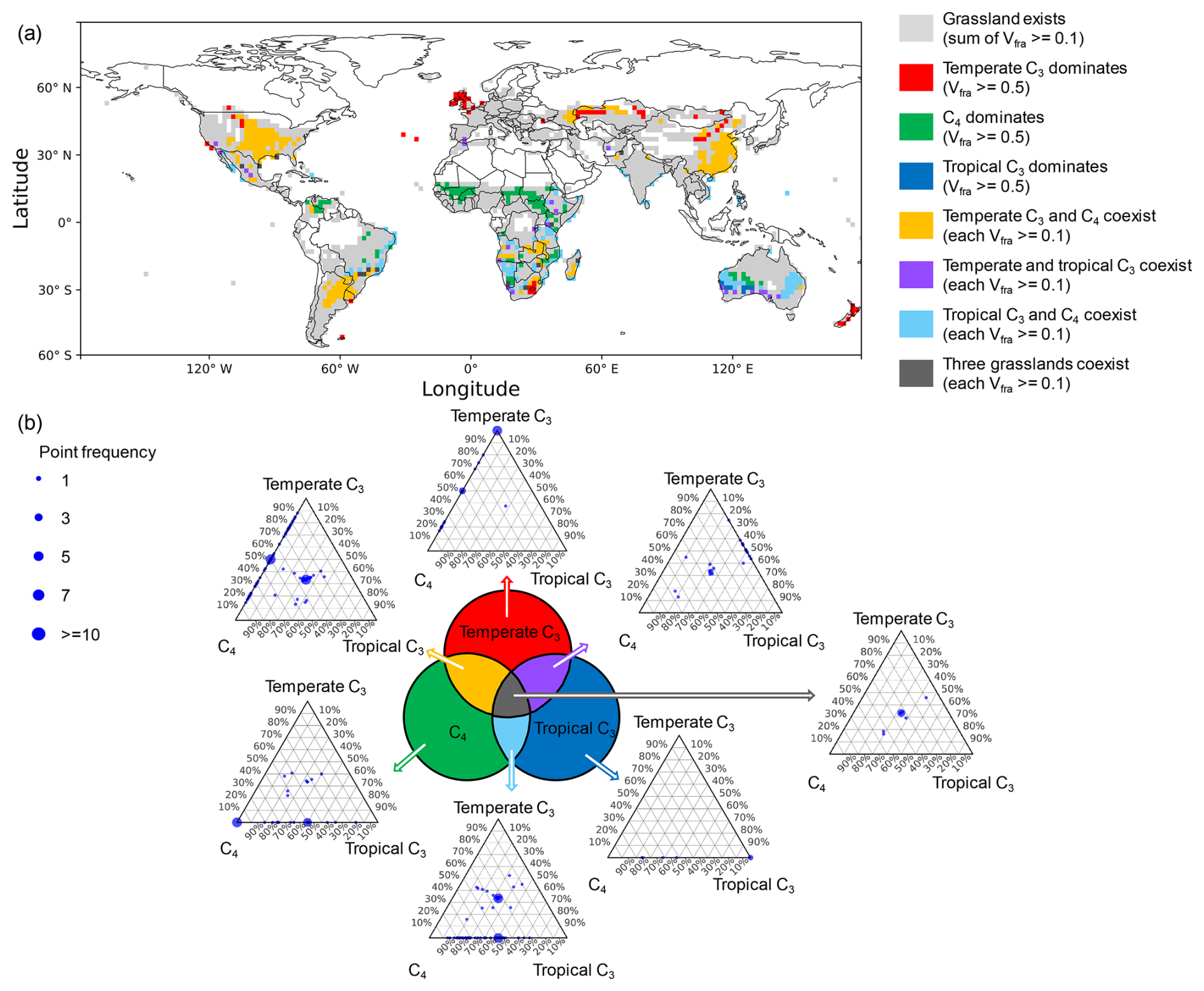
Figure 4 Global distribution of grassland categories and their relative grassland density mixtures. (a) Grassland classification based on fraction of vegetation type (V_fra). Grey areas indicate where the total grassland V_fra is ≥0.1. These areas are further classified into seven categories: (1)t temperate C₃-dominated (V_fra of temperate C₃ grassland ≥ 0.5 while V_fra in other grassland PFTs < 0.1, red); (2) C₄-dominated (V_fra of C₄ grassland ≥ 0.5 while V_fra in other grassland PFTs < 0.1, green); (3) tropical C₃-dominated (V_fra of tropical C₃ grassland ≥ 0.5 while V_fra in other grassland PFTs < 0.1, blue); (4) temperate C₃ and C₄ co-existence (V_fra≥0.1 for both types while V_fra in tropical C₃ grassland  < 0.1, yellow); (5) temperate and tropical C₃ co-existence (V_fra≥0.1 for both types while V_fra in C₄ grassland < 0.1, purple); (6) tropical C₃ and C₄ co-existence (V_fra≥0.1 for both types while V_fra in temperate C₃ grassland < 0.1, cyan); (7) three grassland types co-existence (V_fra≥0.1 for all grassland types, dark grey). (b) Ternary plots showing the relative proportions of normalized grassland density for the three grassland types (temperate C₃, C₄ and tropical C₃) within each grid cell. Each subplot corresponds to one of the seven grassland categories in (a). Point size represents the frequency of occurrence at a given PFT mixture.

The land cover map for each grassland type (Fig. S8) provides information on V_fra. Based on this, grassland categories (Fig. 4a) were classified using the V_fra thresholds introduced in Sect. 2.4. Grid cells with a total V_fra≥0.1 for all grassland types are marked in light grey, representing regions of significant grassland presence. Within these areas, seven distinct grassland categories were identified. Specifically, among these grid cells with grassland presence, 3 % of grid cells were dominated by temperate C₃ grasses (red), 5 % by C₄ grasses (green), and 0.4 % by tropical C₃ grasses (blue). Co-existence patterns included: temperate C₃ and C₄ grasses (12 %, yellow), temperate and tropical C₃ grasses (1 %, purple), tropical C₃ and C₄ grasses (6 %, cyan), and all three grassland types co-existing (0.7 %, dark grey).

Figure 4b shows ternary plots illustrating the grassland density mixtures among the three grass PFTs. In these plots, the position of each point indicates the relative proportion of grassland density from the three grassland PFTs within that grid cell: temperate C₃ (top apex), C₄ (bottom left), and tropical C₃ (bottom right). To achieve this, the densities of the three PFTs in each grid cell were normalized such that their sum equals 1, thereby highlighting their relative contributions. Point size corresponds to the frequency of similar PFT mixtures across grid cells, with larger points indicating higher occurrence. As expected, points tended to cluster near the apex corresponding to the dominant PFT in grid cells where a single grassland type prevailed, reflecting a higher proportional contribution of that PFT to overall grassland density. Deviations occurred where non-dominant PFTs contributed to grassland density but appeared with lower frequency. In cases where two PFTs coexist, points were predominantly distributed along the edges between the respective apices, while for the coexistence of three-PFTs, points shifted toward the centre of the triangle, indicating a more balanced contribution of grassland density among the three grassland types.

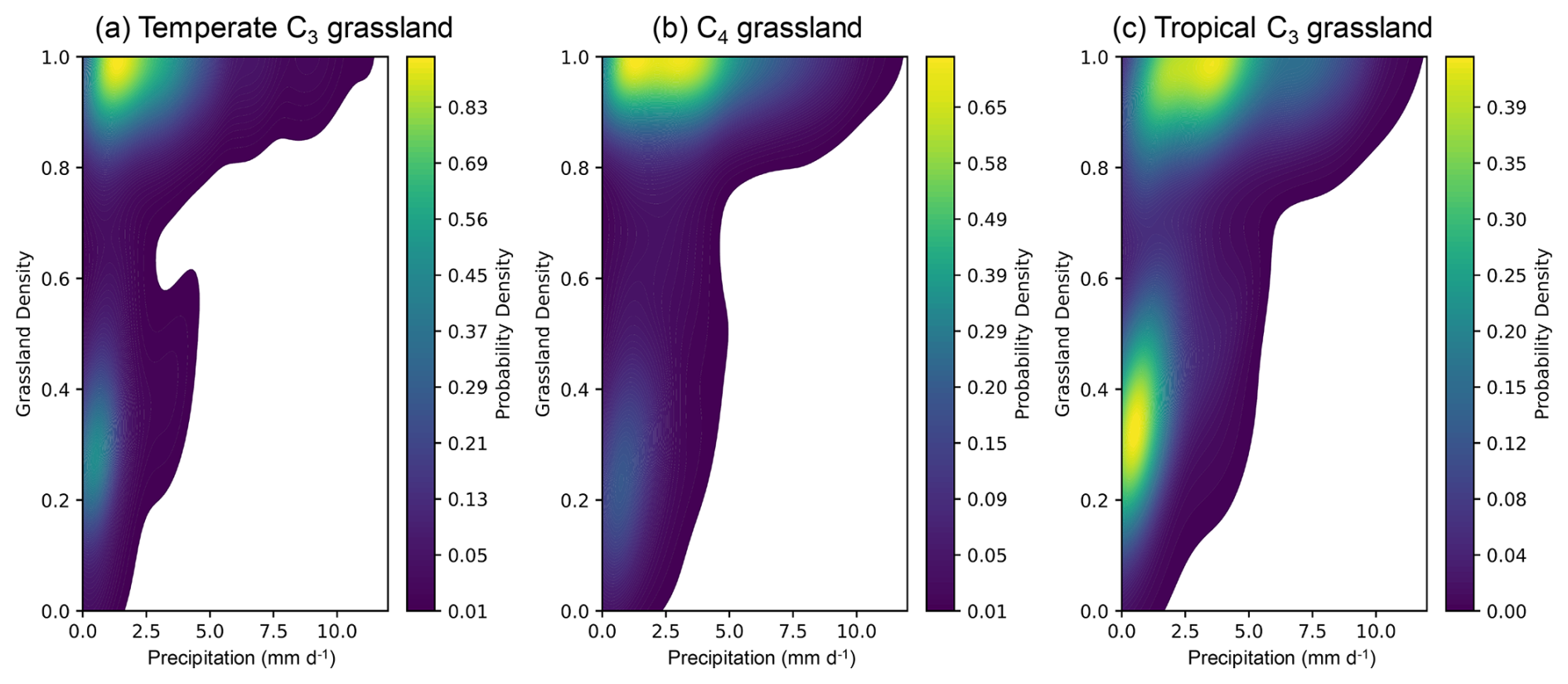
Figure 5 Relationship between precipitation and grassland density. The two-dimensional kernel density estimation (2D KDE) plots illustrate the correlation between precipitation and grassland density for temperate C₃ (a), C₄ (b), and tropical C₃ (c) grasslands. Lighter colours indicate higher probability densities, while darker colours represent lower probability densities. Grassland density and precipitation values were averaged over the period 2004–2020.

Two-dimensional kernel density estimation (2D KDE) plots (Fig. 5) illustrated the distribution of grassland density along the precipitation gradient for three grass PFTs. Grassland density exhibited a positive correlation with precipitation for all three grass PFTs, forming two distinct clusters separated by a grassland density value of approximately 0.7. Above this value, grassland density increased with precipitation. The peak probability density (indicated in yellow) for all grass PFTs occurred at grassland density values between 0.9 and 1, and at precipitation rates ranging from 0.5 to 4 mm d⁻¹. When grassland density was below 0.7, a positive trend with precipitation remained evident, particularly for tropical C₃ grasslands.

3.3 Mortality events simulated in grasslands

The fixed density approach, used in this study as the reference, prescribes the grassland density at unity, implying grasslands are fixed at their maximal density regardless of whether the environmental conditions are favourable. The grassland survival in the model depends on productivity per conceptual individual, which is represented as the gross primary productivity (GPP) per conceptual individual. When this value drops below an arbitrary threshold of 10⁻⁴ g C m⁻² d⁻¹ per conceptual individual, ORCHIDEE considers it insufficient for grassland survival and kills the vegetation. Over the 17-year period (2004–2020), in the fixed density approach, 40 %, 32 %, and 58 % of grid cells in temperate C₃, C₄, and tropical C₃ grasslands, respectively, fell below this critical productivity threshold albeit with different frequencies (Fig. S9a–c). By implementing the dynamic density approach, these proportions decreased to 24 %, 26 %, and 34 %, respectively (Fig. S9d–f).

Over 51 simulation years, the mortality of temperate C₃ grasslands with the dynamic density approach was reduced in 98 % (Fig. 6d) of the grid cells when compared to the fixed density approach (Fig. 6a). Similarly, C₄ grasslands (Fig. 6e) and tropical C₃ grasslands (Fig. 6f) showed a reduction in 97 % and 99 % of the grid cells, respectively. With the dynamic density approach, 51 % of the grid cells in temperate C₃ grasslands experienced zero mortality events over the 51-year simulation period, compared to 55 % for C₄ grasslands and 50 % for tropical C₃ grasslands. The dynamic density approach helped address the high frequency of mortality events simulated with the fixed density approach (Fig. 6a–c), with paired t-tests showing a significant reduction in the mortality for temperate C₃ grasslands (n=1526 grid cells, p<0.001), C₄ grasslands (n=1776 grid cells, p<0.001), and tropical C₃ grasslands (n=1001 grid cells, p<0.001).

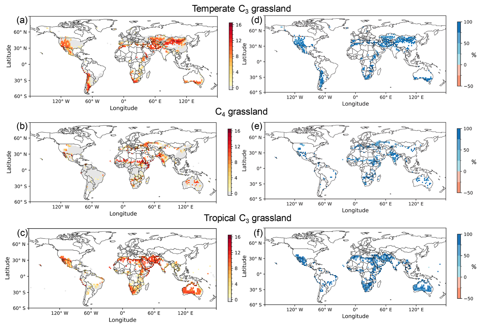
Figure 6 Counts of mortality events using the fixed density approach (a–c) and the relative mortality reduction using the dynamic density approach (d–f) for temperate C₃ grasslands (a, d), C₄ grasslands (b, e), and tropical C₃ grasslands (c, f). The number of mortality events was accumulated over a 51-year test simulation, driven by climate forcing data from 2004 to 2020 and conducted after a 150-year spin-up period that allowed the model to reach equilibrium. The relative reduction was calculated by subtracting the number of mortality events in the dynamic density approach from those in the fixed density approach, and then dividing the result by the number of events in the fixed density approach. Positive values (in blue) signify that the dynamic density approach reduced mortality, while negative values (in red) signify an increase.

Despite applying the dynamic density approach, the mortality events still remained (Fig. S2). Of these, 97 % of mortality cells occurred in “constrained regions” which are in reality not well suited for grassland survival (Sect. 2.5). This result indicates that the simulated mortality is primarily attributable to potential errors in the PFT maps, which incorrectly classified grasslands in regions which are in reality not well suited for grasslands.

3.4 Relationship between aridity and mortality events on grasslands

We examined the correlation between aridity and mortality events for both density approaches over a 51-year simulation driven by climate forcing data from the 2004–2020 period. In the fixed density approach, in which grassland density does not respond to resource availability, mortality events occurred within an aridity range of 0.3 to 1 (Fig. 7a–c) in temperate C₃ grasslands, C₄ grasslands and tropical C₃ grasslands. For the dynamic density approach (Fig. 7d–f), mortality occurred at a higher aridity compared to the fixed density approach (Fig. 7a–c). Specifically, to reach the frequent mortality events (assumed to occur 5 times or more over 51 years, Sect. 2.5), the aridity threshold under the fixed density approach was 0.3 for all three grassland types (Fig. 7a–c). In contrast, the dynamic density approach significantly increased the aridity threshold for reaching frequent mortality events to 0.7 for C₄ grasslands and 0.9 for both temperate and tropical C₃ grasslands (Fig. 7d–f).

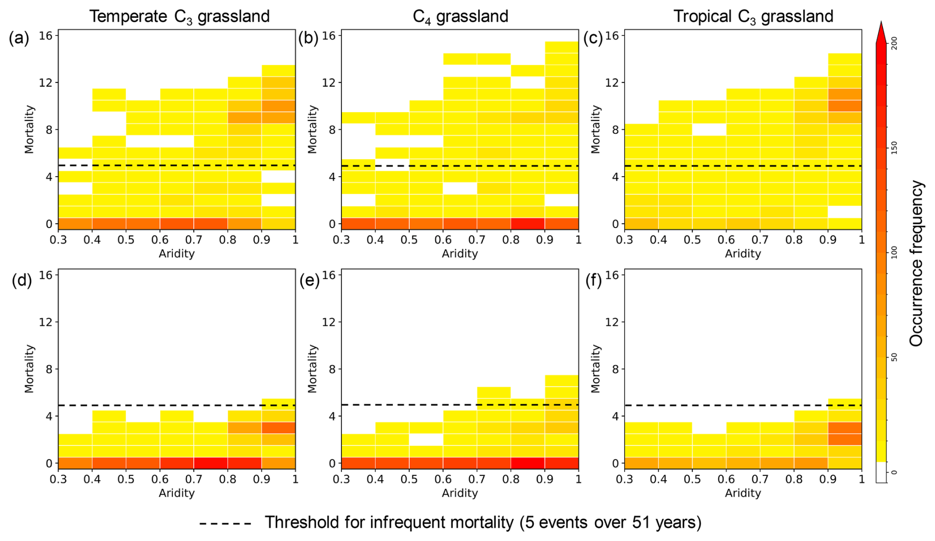
Figure 7 Relationship between aridity and mortality events over three types of grassland. Panels (a)–(c) show the relationship using the fixed density approach, while panels (d)–(f) show it using the dynamic density approach. The grassland types are temperate C₃ (a, d), C₄ (b, e), and tropical C₃ (c, f). The mortality events were accumulated over 51 simulation years, and the aridity was calculated for the same period. The dashed line at five mortality events marks the threshold, separating “infrequent mortality” from more frequent events.

The dynamic density approach effectively suppressed mortality events, particularly under arid conditions. For instance, when aridity exceeds 0.9, fewer than seven mortality events were simulated in the dynamic density approach (Fig. 7d–f). To quantify the overall impact, we aggregated mortality events for 51 simulation years across all grassland PFTs and grid cells. When aridity was lower than 0.9, the total number of mortality events decreased by a factor of 6, from 5872 (fixed density approach) to 999 (dynamic density approach). The reduction reached a factor of 4 under higher aridity (aridity ≥ 0.9), with the event count decreasing from 6123 to 1467.

3.5 Comparison between simulated and observed LAI in grasslands

In this section, we assessed the simulated grassland LAI not merely as a value for direct comparison with observations, but more importantly, as a crucial indicator of improved ecosystem function under the dynamic density approach – specifically, its ability to sustain productivity and reduce mortality.

MODIS remote sensing observations were used to determine the presence of grasslands. Grasslands were considered present in pixels where the MODIS vegetation mask indicated that grassland should be present and where the observed LAI was greater than 0.1 (Tian et al., 2004; Hajj et al., 2014; Lawal et al., 2022). For 60% of the grid cells identified by MODIS as grasslands presence, ORCHIDEE simulated grassland with a LAI > 0.1 in both approaches. Among these grid cells, 64 % showed no mortality events with the fixed density approach. This proportion increased to 86 % with the dynamic density approach. Furthermore, among the grid cells that exhibited mortality with the fixed density approach, 97 % showed a reduction in mortality in the dynamic density approach.

In both approaches, simulated mean annual LAIs were generally lower than observed LAIs in grasslands (Fig. 8a). This underestimation was especially pronounced in South Asia, South America, and Central Africa, with differences ranging from −0.5 to −3 (Fig. 8b and c). Conversely, simulated LAIs were higher than observations (differences of +0.5 to +3) mainly in southwest China and Mongolia. In Australia and southern Africa, the differences were less pronounced. Furthermore, grassland LAI from Sentinel-2 data (2019) was consistent with the LAI simulated by the dynamic density approach in southern Africa and Australia (Wan et al., 2024; Fig. S10). Compared to the fixed density approach, the dynamic density approach resulted in a higher mean annual LAI for 26 % of the grid cells and a lower LAI for the remaining 74 % (Fig. 8d).

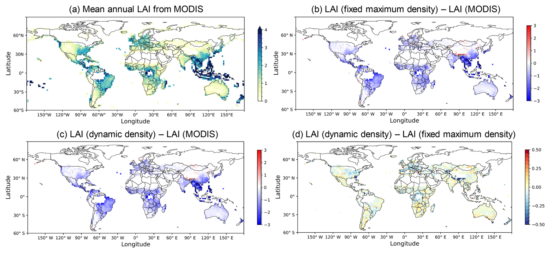
Figure 8 Comparison of simulated and observed mean annual LAI for grasslands averaged from 2004 to 2020. (a) Observed mean annual LAI from MODIS. Differences in mean annual LAI are shown as residual maps: (b) fixed density approach minus MODIS, (c) dynamic density approach minus MODIS, and (d) dynamic density approach minus fixed density approach. The figure and analyses were limited to grid cells where the sum of V_fra values from the three grassland types exceeds 0.1.

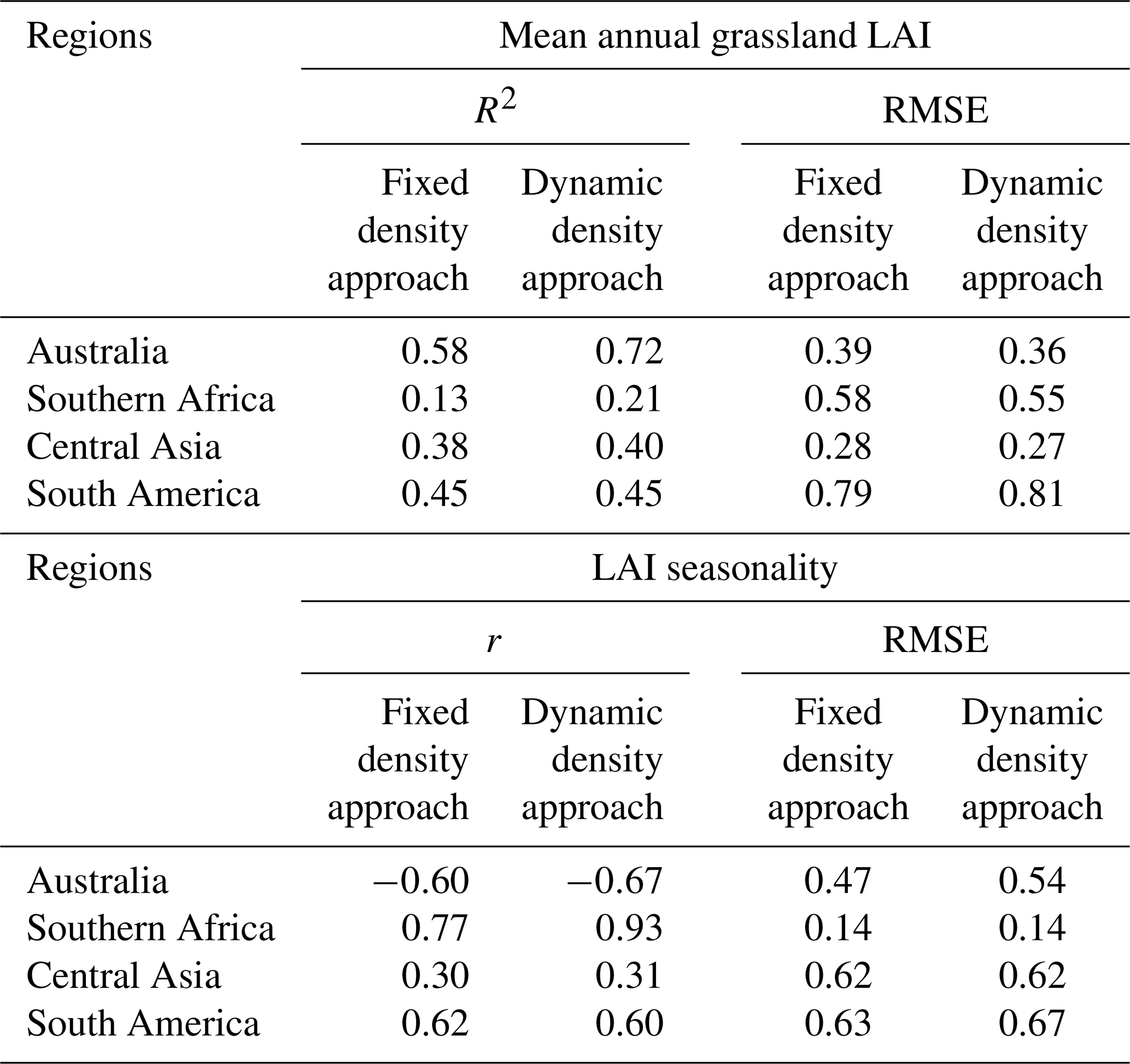
To refine the LAI analysis, a mask was applied to (semi-)arid regions identified by Zomer et al. (2022), focusing on water-stressed environments. Globally, compared with the MODIS dataset (Fig. 8a), the Pearson correlation coefficient (r) increased from 0.51 to 0.56, and the RMSE decreased from 0.60 to 0.59 when transitioning from the fixed density to the dynamic density approach. Spatially, statistical analysis was conducted for the four representative semi-arid regions: Australia, southern Africa, Central Asia, and South America (Fig. S11a), which were chosen as they represent the large contiguous grassland ecosystems within the semi-arid domain on their respective continents. In all four regions, the coefficient of determination (R²) improved or remained unchanged under the dynamic density approach (Fig. S11b–e, Table 2), while RMSE decreased in three regions (Australia, Central Asia, and southern Africa). Moreover, the dynamic density approach enhanced the seasonal dynamics in southern Africa (Fig. S12b, Table 2), successfully capturing the dry-season LAI minimum (August–October) that the fixed density approach failed to reproduce. The new dynamic density approach increased the seasonal correlation (r) with MODIS from 0.77 to 0.93, compared to the fixed density approach. In contrast, seasonality in Australia (Fig. S12a) and South America (Fig. S12d) did not show improvements (Table 2).

Table 2 Statistical comparison of simulated grassland LAI (from this study) against MODIS LAI across four regions: Australia, southern Africa, Central Asia, and South America. Statistics include the coefficient of determination (R²) and RMSE for mean annual LAI, and Pearson's r and RMSE for LAI seasonality.

The ratio of the relative difference in LAI to the relative difference in mortality between the two approaches was computed at the level of PFTs (Fig. 9). The analysis focused on grid cells where: (1) the grassland density was less than unity in the dynamic density approach, and (2) mortality occurred with the fixed density approach. The first condition was chosen because LAI is influenced by density only when it is below unity (according to Eq. 7). The second condition was applied to illustrate mortality reduction in the dynamic density approach and to prevent invalid ratio calculations. A ratio lower than 1 indicates that LAI reduces very little while mortality decreases significantly, suggesting that plant productivity is allocated in a way that better supports vegetation fitness. In contrast, a ratio greater than 1 reflects a substantial decrease in LAI with only a small reduction in mortality. The results showed that 84 %, 81 % and 75 % grid cells in temperate C₃, C₄, and tropical C₃ grasslands, respectively, had ratios below 1 (Fig. 9).

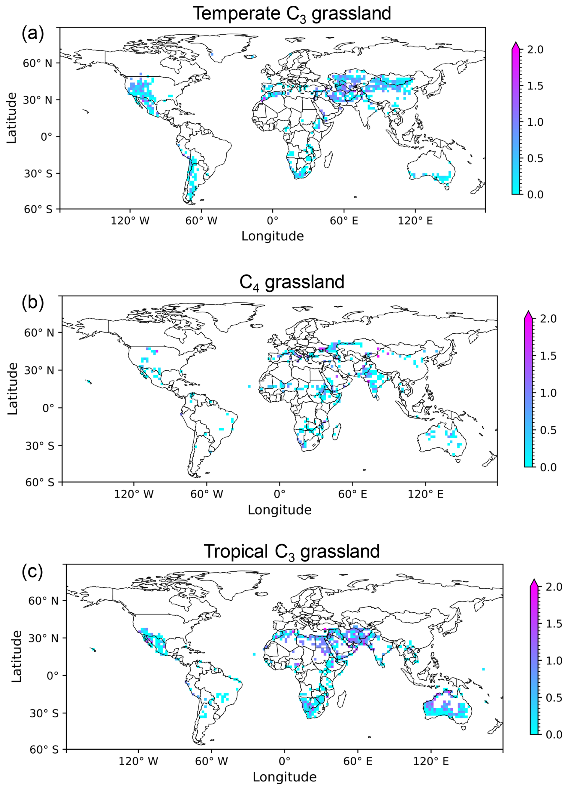
Figure 9 Ratio of the relative difference in LAI to the relative difference in mortality events between the fixed and dynamic density approaches for temperate C₃ grasslands (a), C₄ grasslands (b), and tropical C₃ grasslands (c). The relative difference was calculated by subtracting the value in the fixed density approach from that in the dynamic density approach, then dividing by the value in the fixed density approach. To ensure valid calculations, both LAI and mortality values were required to be greater than zero in the fixed density approach. Mortality events were accumulated over a 17-year period for this analysis, and LAI values were averaged over the same time span.

4 Discussion

4.1 The implementation of dynamic grassland density

In ORCHIDEE, the recruitment scheme is represented as asexual recruitment, based on the assumption that grasslands are dominated by perennial species. Most perennial grasses primarily reproduce asexually through clonal stems derived from belowground tissues, while sexual reproduction via seeds plays a comparatively smaller role (Blair et al., 2013). In contrast, annual plants rely exclusively on seeds for yearly regeneration. While our model's assumption captures the dominant strategy in perennial grasslands, we acknowledge it as a limitation: the model may underperform in ecosystems where sexual reproduction and persistent seed banks are the primary drivers of recruitment.

Despite this simplification, this study introduces a novel approach in ORCHIDEE r9010 to calculate grassland density as a trade-off between the carbon pools (e.g., reserve and labile carbon) in conceptual individuals and the total number of conceptual individuals. This differs from other models that simulate a dynamic grassland density, such as the spatial patch dynamics model PATCHMOD (Wu and Levin, 1994) and the individual and process-based grassland model GRASSMIND (Wirth et al., 2021), which simulate more explicit demographic processes. By contrast, our simplified yet effective approach (see results and discussion below) allows dynamic grassland density to be simulated at the typical scale of a grid cell in the land surface model ORCHIDEE, i.e., between 50 km × 50 km and 200 km × 200 km, enabling a global and computationally efficient representation of grassland dynamics.

The evaluation against five case studies (Table 1) gives confidence in the model's ability to represent grassland density across different grass PFTs and locations. The close agreement at all the five sites suggests our model accurately captures the central tendency of grassland density. Despite these encouraging results, this evaluation should be interpreted with caution due to several key uncertainties. The primary challenge is the conceptual mismatch between our simulated “density” and the observational metrics. The mismatch was mitigated by selecting the closest available conceptual analogues (Sect. 2.3). However, the discrepancies cannot be fully eliminated. For example, in the Australian grass-shrub community (Melville et al., 2019), the field-based metric unavoidably includes shrubs, thus resulting in higher values compared to a pure grassland ecosystem. While the close agreement (Table 1) suggests the dynamic density approach captured the dominant grass trend, the shrublands in Australia might also be misclassified as grasslands in the PFT maps in ORCHIDEE, which would lead to our model simulating grasslands in the shrub-contaminated areas. This alignment may therefore stem partly from this PFT misclassification. In addition, the scale mismatch between plot-level field data and the model's coarse grid-cell resolution is another source of uncertainty, particularly in heterogeneous landscapes like the Mongolian Plateau. Despite this spatial discrepancy, the result that our simulated value range aligned with the observed range suggests the new approach captures the ecological gradient across different steppes: with higher values in meadow steppe, medium values in typical steppe, and lower values in desert steppe (Booth et al., 2005; Dusseux et al., 2014; John et al., 2018; Melville et al., 2019; Diatta et al., 2023).

As shown in the results (Sect. 3.2), the direct FVC comparison against the FCOVER satellite product (Copernicus Land Monitoring Service, 2020) also supported the new dynamic density approach, which improved both spatial correlation (r) and RMSE. There are two main caveats in this comparison, which likely explain the deviation from observations: (1) in (semi-)arid regions, the FCOVER product includes all green vegetation (e.g., shrubs, crops), whereas our calculation was focused only on the grassland PFTs we improved. (2) The current model does not yet account for key disturbances like grazing or fire, which are known to affect FVC and are implicitly included in the satellite observations (Chang et al., 2016, 2021). Nevertheless, the fact that our new scheme showed a clear improvement despite these known mismatches underscores the robustness of the new dynamic density approach.

Despite the evidence of model improvements, the global observations of grassland density remain challenging due to incomplete and inconsistent datasets. Grassland density is known to be strongly influenced by resource availability, particularly water (Schneider et al., 2008; John et al., 2018). Our results demonstrate that ORCHIDEE effectively captures a positive relationship between precipitation and simulated grassland density, with density declining notably under low annual precipitation. For ORCHIDEE, this relationship is an emerging property, as a relationship between precipitation and grassland density was not coded as such. It can therefore be concluded that the proposed approach is able to simulate grassland density as the outcome of essential processes such as competition, survival, and mortality under varying resource availability (Deblauwe et al., 2008).

Additionally, such a precipitation-density relationship is also a valuable diagnostic indicator to identify and evaluate potential biases in model behaviour. In some cases, the model maintained maximum grassland density despite scarce precipitation. For instance, while C₄ grasses are known for their resilience to extreme conditions (Taylor et al., 2010), our model simulates their density at maximum levels even when precipitation falls below 1 mm d⁻¹ – an overly optimistic outcome. As part of this study, we have already recalibrated the dynamic density approach – with a focus on C₄ grasslands in southern Africa (Figs. S5 and S6) – to increase the model's sensitivity to low precipitation. Applying this recalibration globally leads to a generally improved performance, with the model capturing a plausible emergent relationship between precipitation and density in most grasslands. Despite this improvement, the aforementioned counterintuitive result is not entirely eliminated. Therefore, future model investigations should focus on understanding the conditions that lead to this result, and on developing more adaptive parameterizations.

While the use of the fraction of vegetation type (V_fra) as a proxy offers a method to evaluate grassland density, it also introduces uncertainties. If the land cover map is accurate, high V_fra could be interpreted as an indicator of favourable climatic conditions for a given PFT. Low V_fra may reflect unfavourable climatic conditions, but it may also be attributed to non-climatic factors, which are not considered in this study, such as fire, grazing, and human management (Chang et al., 2016, 2021). In addition, the land cover map may overlook subpixel vegetation structure of grasslands. For example, an area with a homogeneous mixture of grass and bare soil may be classified entirely as grassland with a high V_fra, even though the actual grassland density might be lower due to the sparse vegetation. Conversely, in locations where a remote sensing product can resolve distinct patches of grass and bare soil, only the grass-covered areas may be identified as grassland, while adjacent bare soil is classified as separate bare soil. In such cases, grassland density may be high, but V_fra appears low. This could also account for the cases where PFTs with negligible V_fra still exhibited substantial grassland density. It highlights the importance of considering bare soil distribution in the classification of grassland PFTs from land cover maps, particularly when interpreting or validating grassland density.

In this study, we introduced and evaluated a novel, computationally efficient approach to simulate dynamic grassland density within ORCHIDEE. Our analysis highlights two primary avenues for future improvement: refining the model's internal process-based responses and better constraining uncertainties arising from external drivers. Internally, the counterintuitive persistence of grasses under extreme water stress (e.g., C₄ grasses) warrants refining water stress parameters and reserve and labile carbon targets to better capture: (1) the response of grasslands to climate and (2) the density of co-existing grassland PFTs. Externally, acknowledging the limitations of proxies like V_fra and the influence of non-climatic factors underscores the importance of incorporating disturbances such as agricultural practices and grazing. Addressing these internal and external factors will be crucial for advancing ORCHIDEE's capability to accurately simulate the geographical distribution and dynamic density of global grasslands.

4.2 Reduced mortality events with the dynamic density approach

The vegetation in semi-arid regions, where extreme conditions are unfavourable for growth, tends to have low productivity and is prone to mortality events (Fig. S9; Wang et al., 2022). In ORCHIDEE, carbon starvation could result in grassland mortality during lasting droughts. Following a drought, the model establishes a new grassland, at the beginning of the next growing season. However, if mortality events are frequent (in this study assumed as five or more events over 51 simulation years), it suggests that the grasslands are not viable in ORCHIDEE, which contradicts the vegetation map that indicates that grassland is present at that location. Therefore, frequent mortality events of grassland might indicate a shortcoming in either the model or the PFT map. In the dynamic density approach, more grid cells with grasslands were able to maintain growth compared to the fixed density approach (Fig. S9), resulting in a significant reduction in mortality events over grasslands.

To separate model limitations from shortcomings in the PFT map, we therefore identified simulated mortality events that occurred in constrained regions (see Sect. 2.5). Except for these regions, grasslands are expected to survive in the corresponding ORCHIDEE grid cell, and the mortality in ORCHIDEE should occur infrequently and be mainly driven by drought. The finding that 97 % of the grid cells with simulated mortality occurred within these constrained regions suggests that these mortality events are less likely an artefact of the model's new dynamic density approach, and more likely a consequence of potential errors in the PFT map (Poulter et al., 2011; Reinhart et al., 2022), where non-viable land may be misclassified as grassland. Consequently, these PFT maps derived from satellite-based products should be used with caution, as such potential misclassifications could be a primary driver of unrealistic mortality in the simulation.

The remaining occurrence of mortality events with the dynamic density approach suggests that in (semi-)arid regions, simulated plant resistance to water stress might be underestimated during drought, leading to too early mortality once soil moisture falls below the wilting point. In ORCHIDEE, the wilting point is defined as a threshold in volumetric soil water content, below which leaves reach irreversible wilting (Wiecheteck et al., 2020). This threshold is not PFT-specific; instead, it is determined solely by soil properties, with different soil textures (e.g., loamy sand vs. loam) assigned different wilting point values in the model. However, recent studies indicate that the wilting point is more accurately characterized as a plant-specific hydraulic trait rather than a universal soil property (Bartlett et al., 2016; Marchin et al., 2020). For instance, some arid-adapted species can survive at soil water potentials below the conventional soil-defined wilting point (Bartlett et al., 2012; Bartlett et al., 2016). Consequently, the model's reliance on a conservative, soil-based threshold – rather than PFT-specific hydraulic traits that reflect true drought tolerance (Bartlett et al., 2016) – likely leads to mortality events earlier than observed.

Furthermore, adjusting photosynthetic capacity, stomatal conductance and the wilting point as a function of the environment (Chebbo et al., 2025) may better reflect plant resilience to prolonged water stress. Since ORCHIDEE model uses fixed parameter values within a PFT, a potential improvement would be to introduce spatial variation in these traits to reflect species variation across climate gradients. One practical approach would be to compute these parameters as functions of long-term mean precipitation, thereby distinguishing between dryer and wetter climatic regions. This would be consistent with the evidence that perennial grasses can modify their drought-tolerant traits to enhance survival under extreme dry conditions (Norton et al., 2016; Guo et al., 2017). For example, species like Danthonia californica, Geranium dissectum and Alopecurus pratensis dominate in wet regions, while Lupinus bicolor, Bromus hordeaceus and Cenchrus ciliaris are common in dry regions (Gubsch et al., 2011; Sandel et al., 2011; Kattge et al., 2020). In addition to spatial differentiation, another improvement would be to allow temporal variation in these parameters so that they can adjust to changes in growing conditions, capturing processes of acclimation or longer-term adaptation. Implementing such temporal dynamics, however, is more challenging – especially in already extremely dry regions – because it remains uncertain whether species can further adjust their physiology or whether they are able to survive near fundamental physiological limits (Vandegeer et al., 2020). Nonetheless, incorporating spatial (species variation) and temporal (acclimation and adaptation) adjustments would provide a more realistic representation of plant responses to drought in ORCHIDEE.

4.3 The aridity threshold for frequent mortality events in grasslands

To facilitate the analysis in this study, “frequent mortality” is defined as occurring five times or more over a 51-year simulation period, based on ecological records of widespread, drought-driven mortality in perennial grasslands (Blair et al., 2013; Bodner and Robles, 2017). While this provides a reasonable benchmark, we acknowledge that it is a simplified assumption. Future research could further evaluate the robustness of our findings across a range of threshold values and ecosystems.

Given the same high aridity, grasslands tend to die less frequently in the dynamic density approach compared to the fixed density approach. The sensitivity to drought was not coded as such but emerged from the model's dynamics, suggesting that adjusting vegetation density is an effective strategy for adapting to difficult growing conditions. This is consistent with the observed spatial self-organisation in grasslands that has been explained as an adaptation to water availability (Rietkerk et al., 2002).

Aridities of 0.54, 0.69, and 0.83 have been found to result in vegetation decline, soil degradation, and systemic breakdown respectively (Berdugo et al., 2020). With the dynamic density approach, frequent mortality events were triggered only at the aridity thresholds: 0.7 for C₄ grasslands, and 0.9 for temperate and tropical C₃ grasslands. This finding aligns with the aridity threshold for systemic breakdowns (0.83) reported by Berdugo et al. (2020). The dynamic density approach thus reproduced a realistic response of grasslands to aridity. Moreover, if the thresholds reported by Berdugo et al. (2020) are globally valid, this could suggest an inconsistency in the land cover maps used by ORCHIDEE where 30 % of the grasslands are prescribed at locations with an aridity exceeding 0.83. This threshold was also used to judge the contribution of potential PFT map errors to the remaining mortality events (Sect. 2.5, Fig. S2). At these locations, the mortality of the grassland PFTs might be a realistic representation of grassland ecology. In arid regions, drought-adapted species such as succulents (Buckland et al., 2023), halophytes (Hussain et al., 2023) and phreatophytes (Sommer and Froend, 2014) are expected instead of grasses. None of these are explicitly accounted for in the PFT maps. If their vegetation cover is sufficient to be seen from space, these vegetation types might all be classified as grasslands in the PFT map (Poulter et al., 2015).

4.4 Implications of grassland LAI in ORCHIDEE

With the dynamic density approach, simulated mean annual LAI is expected to be lower than that in the fixed density approach. This is because, according to Eq. (7), LAI is a function of both the leaf biomass of a conceptual individual and the number of conceptual individuals. Our study demonstrated that 74 % of the grid cells had a lower mean annual LAI when dynamic grassland density was accounted for (Fig. 8d). A 26 % proportion of grid cells showed higher simulated LAI values with the dynamic density approach, which may be attributed to a trade-off effect (Jongejans et al., 2006). On one hand, grassland density is reduced to alleviate growth stress caused by limited resource availability (Harper, 1977). On the other hand, decreased plant density in resource-limited conditions (e.g., water, nutrients) alleviates competition among plants and improves individual biomass growth (Springer, 2021). Although grassland density is lower, the individual leaf biomass increases due to improved growing conditions. As a consequence, this trade-off may explain the slightly higher LAI with the dynamic density approach for these 26 % proportion of grid cells.

The global and regional quantitative assessment against the MODIS dataset demonstrates that the dynamic density approach yields consistent, albeit modest improvements in grassland LAI (Figs. S11 and S12). However, this analysis also reveals that the overall global improvement is minor, and that the issue of LAI seasonality persists. It is important to note that LAI seasonality is driven by the phenology subroutine in ORCHIDEE, which was not modified by our new dynamic density approach. Improving this phenology remains a separate, long-standing challenge in Earth System Models. This underlying issue is relevant, though, as these persistent phenological issues likely contribute to the remaining mortality events in our simulations.

The underestimation of grassland LAI in ORCHIDEE compared to MODIS was not fully resolved with the dynamic density approach. This remaining model-data discrepancy likely stems from uncertainties in both the observational data and the model structure. From the MODIS perspective, the derivation of the LAI product using a global-scale process model by MODIS may affect its accuracy and lead to an overestimation of LAI by approximately 2 %–15 % (Fensholt et al., 2004). On the ORCHIDEE side, hydrological processes are the key factor (MacBean et al., 2020); the underestimation might be partially explained by the runoff-to-precipitation ratio (Critchley et al., 2013) and the representation of evapotranspiration (Burchard-Levine et al., 2022) under water-limited conditions. Furthermore, uncertainties in key biophysical parameters, such as the Specific Leaf Area (SLA) used to convert leaf biomass to LAI, may also constrain simulated leaf growth. Addressing this issue likely requires a multi-faceted strategy; future work should therefore focus on improving surface hydrology representation, refining plant functional parameters via data assimilation, and expanding model evaluation using a broader set of remote sensing products.

This study goes beyond a direct comparison of simulated and observed LAI by exploring how observed LAI can inform on the likelihood that grassland is present at a given location. While land cover maps may include classification uncertainties, incorporating observational LAI – particularly when LAI exceeds 0.1 – improves the reliability of mortality event analyses. In the dynamic density approach, the low frequency of mortality in regions with observed LAI from MODIS > 0.1 suggests that grasslands can persist by adjusting their density to current climatic conditions (Tian et al., 2004; Hajj et al., 2014; Lawal et al., 2022). Therefore, the need for re-establishing grasslands by the model is greatly reduced. In contrast, the fixed density approach leads to frequent mortality events in some regions, followed by a substantial influx of carbon from the biomass of the re-established grassland. As a result, model outputs may suggest unrealistically high productivity solely due to the frequent need to re-establish the vegetation. By comparison, the dynamic density approach ensures the survival of the grassland community by allowing for density reduction, at the cost of potentially lower productivity and LAI values compared to the fixed density approach. However, the ratio between the relative reductions in LAI and mortality (Fig. 9) indicates a beneficial trade-off, where the reduction in LAI is less pronounced than the reduction in mortality events for the majority of grid cells.

4.5 Consequences for PFT maps

Poulter et al. (2015) provide a cross-walking table that helps assign land cover classes from remote sensing products into PFTs used in ORCHIDEE. However, such an approach may introduce inconsistencies, as the dynamic density approach in this study simulates a bare soil fraction within grasslands based on grassland density. The areas classified as bare soil may in reality contain sparse or seasonal vegetation that should be represented by a grassland or shrubland PFT, especially in semi-arid systems. Future model implementations could improve realism by replacing the fixed “bare soil” PFT with a dynamic representation of bare ground. In addition, the presence of mapped grasslands in regions that are classified as hyper-arid (Zomer et al., 2022), exhibit extremely low observed LAI, or exceed the ecological threshold for “systemic breakdown” (Berdugo et al., 2020) highlights a critical uncertainty in these external PFT maps. This finding underscores the need to investigate whether grasslands can realistically persist in these regions. Improving the realism of the land cover maps would subsequently reduce potential biases in vegetation dynamics and mortality events in ORCHIDEE, especially in dryland ecosystems where vegetation is sparse but not entirely absent.

5 Conclusions and future perspectives

The default grassland representation in ORCHIDEE, which applies a fixed density, does not adequately reflect the sparse and low-density vegetation typically found in resource-limited regions, such as semi-arid areas. This mismatch – between a static high density in the model and the limited ecological capacity to sustain such density under low resource availability – results in frequent and unrealistic mortality events. Therefore, this study proposed a simple yet effective approach to simulate a dynamic grassland density in the land surface model ORCHIDEE. The core of this approach is to link grassland density directly to the plant's carbon status, which serves as an integrated indicator of vegetation vitality. Specifically, grassland density decreases when reserve and labile carbon in the plant are insufficient, while it increases when reserve, labile and fruit carbon are abundant (Fig. 2).

Compared to the fixed density approach, the implementation of dynamic grassland density in ORCHIDEE led to several notable improvements: (1) grassland density is now simulated within the range of 0.05–1 globally, aligning with five regional case studies, leading to a better representation of bare soil in grasslands, and positively correlating with annual precipitation as an emerging property. (2) Mortality events are substantially reduced over grasslands in ORCHIDEE. (3) Incorporating dynamic grassland density raises the aridity thresholds for frequent mortality events in grasslands, with this behaviour emerging from the new approach rather than being explicitly prescribed. (4) The lower mean annual LAI values simulated by the dynamic density approach modestly improve model agreement with observations both globally and regionally, and maintain a realistic level of ecosystem productivity, while the approach dramatically reduces grassland mortality, thereby enhancing the model's ecological realism. (5) The dynamic density approach eliminates the need to assign arbitrary bare soil fractions when constructing PFT maps, as the bare soil fraction emerges dynamically from the simulation, thereby improving the realism and consistency of land cover representation.

Furthermore, the improvements pave the way for estimating the dust emission from bare soil in semi-arid grasslands. Integrating this capability will enhance dust emission estimates and provide a more comprehensive understanding of land–atmosphere feedbacks in Earth System Models (Fig. 1c).

This study also suggests several areas where grassland simulations in ORCHIDEE could be improved: (1) refining the phenological processes and parameters for C₄ grasslands, including adjustments to reserve and labile carbon targets, as well as optimization of parameters in the water stress function. (2) Developing a more robust mechanism for triggering mortality events in grasslands, especially under extreme climate conditions. (3) Improving the parametrization of hydrology and phenology to enhance LAI simulation. (4) Enhancing vegetation classification in ORCHIDEE by incorporating more accurate vegetation maps, and explicitly representing sparse grasslands or mixed bare soil and vegetation areas in semi-arid regions, except in regions that are fully bare such as deserts.