rsofun v5.1: a model-data integration framework for simulating ecosystem processes

Mechanistic vegetation models serve to estimate terrestrial carbon fluxes and climate impacts on ecosystems across diverse biotic and abiotic conditions. Systematically informing them with data is key for enhancing their predictive accuracy and estimating uncertainty. Here, we demonstrate and evaluate the Simulating Optimal FUNctioning (rsofun) R package, which provides a computationally efficient implementation of the P-model for site-scale simulations of ecosystem photosynthesis and the acclimation of photosynthetic traits, complemented with functionalities for Bayesian model-data integration and the estimation of model parameters and prediction uncertainty. We estimated model parameters simultaneously from observed time series of ecosystem gross primary productivity (GPP), and from globally distributed data on leaf carbon-13 isotopic discrimination (Δ¹³C) and the ratio of the maximum biochemical rates of carboxylation to electron transport ($V_{\mathrm{cmax}}/J_{\max }$). The multi-target calibration yielded unbiased predictions for all variables simultaneously and produced similar distributions of prediction–observation residuals for both calibration and out-of-sample test data, indicating that the model generalises robustly across diverse environments. We found that a step-wise approach to successive model integration and calibration yielded best results, and that correlations among parameters related to the representation of water stress effects underpinned non-robust parameter estimations. This likely indicates a dominant source of model structural uncertainty related to the representation of the response of photosynthesis to dry conditions in soil and air.

1 Introduction

The modelling of land ecosystem processes and structure, water, and carbon fluxes relies on both mechanistic and statistical approaches (Dietze et al., 2018; Hartig et al., 2012; Van Oijen et al., 2005). Mechanistic models are formulated as mathematical descriptions of functional relationships between the abiotic environment and ecosystem states, rates, and dynamics. These descriptions reflect available theory and general empirical patterns and provide a means for translating hypotheses about governing principles and causal relationships into testable predictions (Marquet et al., 2014), and for upscaling model-based estimates in geographical space and to novel environmental conditions. However, mechanistic models rely also on empirical descriptions of processes at varying levels of abstraction.

Mechanistic models have model parameters that are either specified or fitted to data. A great advantage of mechanistic models is that they explicitly link known physical constants with process representations (e.g., molecular mass of CO₂ for diffusion and assimilation, or the gravitational constant and viscosity of water for its transport and transpiration). Other parameters may be specified based on independent measurements under controlled conditions (e.g., the activation energy of Arrhenius-type metabolic rates), or represent measurable plant functional traits, taken as constant over time and within plant functional types (PFTs – the basic unit in mechanistic vegetation models). Both types of parameters have traditionally been directly specified in models (“direct parameterization”, Hartig et al., 2012). Yet other model parameters may not be directly observable and describe processes that are not explicitly resolved but can be described at a higher level of abstraction. Such parameters are often fitted to observational data such that the agreement between one (or several) related model predictions and observations is optimised. Parameter estimation for mechanistic vegetation models typically employs generic optimization algorithms or Bayesian statistical approaches and is often used to specify diverse types of parameters (except for universal physical constants). Bayesian methods have the advantage that they enable a systematic assessment of the correlation structure among multiple fitted parameters, provide a means to consider uncertainty in inputs, observations, models, and available prior information, generate probabilistic parameter estimations and model predictions, and provide a basis to quantify the constraints by various calibration target data and to identify errors arising from model structural choices (Bagnara et al., 2015; Dietze et al., 2018; Hartig et al., 2012; van Oijen, 2017; Raj et al., 2016; Van Oijen et al., 2005; Xiao et al., 2019).

As the number of parameters increases in state-of-the-art mechanistic vegetation models, taking into account multiple PFTs and ecosystem components (e.g. soil, microbes, hydrology), larger amounts of data and computing resources are required to fully explore the parameter space (Hartig et al., 2012). This poses a limitation for systematic model-data integration and Bayesian parameter estimation. Eco-evolutionary optimality (EEO) principles have been proposed for reducing model complexity and for a robust grounding of models in governing principles (Franklin et al., 2020; Harrison et al., 2021). They enable parameter-sparse representations, limit the distinction of separate PFTs, and may enable better model generalisations to novel environmental regimes. As such EEO principles make predictions of plant functional traits that would otherwise have to be prescribed – typically as temporally fixed model parameters. Parameters in EEO models are considered to be universally valid, e.g., across different PFTs. Ideally, they represent known physical constants or quantities that can be measured independently. However, not all can be measured directly, e.g., the marginal cost of water in Cowan and Farquhar (1977), or the unit cost ratio in Prentice et al. (2014) and need to be fitted to data.

The P-model (Prentice et al., 2014; Wang et al., 2017; Stocker et al., 2020) is an example of an EEO-guided model for terrestrial photosynthesis and its acclimation. It avoids the requirement for prescribing PFT-specific parameters of photosynthesis and stomatal regulation but instead predicts them from universal EEO principles for the full range of environmental conditions across the Earth's (C₃ photosynthesis-dominated) biomes. Through its representation of the vegetation as a big leaf (Bonan et al., 2021; De Pury and Farquhar, 1997), it represents the scaling between leaf traits and ecosystem-level photosynthetic CO₂ uptake (gross primary productivity, GPP). However, despite its foundation on EEO theory and resulting parameter-sparseness, a small set of model parameters remains (Stocker et al., 2020) (Table 2) and must be fitted to data.

Here, we explore the respective constraints provided by ecosystem-level fluxes and leaf-level traits for a probabilistic (Bayesian) multi-target estimation of the P-model parameters. The selection of observational target data types is motivated by their known effectiveness in model calibration and parameter estimation from previous work (Prentice et al., 2014; Wang et al., 2017; Stocker et al., 2020). Specifically, we use observations-based GPP time series from multiple eddy covariance measurement sites, and compilations of globally distributed measurements of leaf traits, including the leaf carbon isotopic fractionation relative to the atmosphere (Δ¹³C, hereafter shortened to Δ), and the ratio of the maximum biochemical rate of carboxylation to electron transport ($V_{\mathrm{cmax}}/J_{\max }\equiv \mathrm{VJ}$). Data from these two leaf traits have previously been used for independently estimating separate model parameters in the P-model (Wang et al., 2017). In Stocker et al. (2020), these independently estimated model parameters where then specified for model simulations (direct parametrization), and were not subject to model parameter calibration. Here, we demonstrate how the combined consideration of diverse data types within a Bayesian model-data integration framework – combining ecosystem flux data and leaf traits data – enables the simultaneous estimation of a comprehensive set model parameters that control functional dependencies of processes at multiple organisational levels – from the leaf to the canopy. This enables a better understanding of interdependencies between model parameters and a more reliable estimation of model prediction uncertainty.

Unbalanced observations of multiple calibration targets can lead to parameter estimates that compensate structural errors in the model, as shown previously with synthetic data (MacBean et al., 2016; Oberpriller et al., 2021; Cameron et al., 2022). We are therefore interested in the questions (i) if the P-model can be calibrated in a consistent manner to these targets resulting in unbiased parameter estimates (relative to expected ranges based on our process-based interpretation of each parameter), and (ii) if the calibrated model generates unbiased predictions with consistent precision on independent test data set.

We start by providing a brief description of the P-model and introduce the P-model implementation in the Simulating Optimal FUNctioning rsofun version v5.1 modelling framework, made available as an R package (Stocker et al., 2025). A more comprehensive description of the P-model can be found in Stocker et al. (2020). rsofun implements the P-model and its connection to data through Bayesian parameter optimisation and analysis. We demonstrate the functionalities implemented in and accessible through rsofun with different calibration setups – i.e., different combinations of model parameters subjected to Bayesian calibration and different observational data types used for calibration. Alternative calibration setups serve to elucidate the role of different observations in constraining estimates for different model parameters. rsofun functionalities demonstrated here include the flexible specification of likelihood functions for connecting model predictions to specific data types, Bayesian model calibration using Monte Carlo Markov Chain sampling, the analysis of posterior distributions of estimated parameters, and the estimation of prediction uncertainty, probabilistic predictions of GPP, VJ, and Δ, and their evaluation against out-of-sample test data.

2 Methods

2.1 P-model description

The P-model predicts the acclimation of leaf-level photosynthesis to a (slowly varying) environment based on EEO principles. It thereby yields a parameter-sparse representation of ecosystem-level quantities, generalising across (C₃ photosynthesis-dominated) vegetation types and biomes. The P-model combines established theory for C₃ photosynthesis following the Farquhar–von Caemmerer–Berry (FvCB) model (Farquhar et al., 1980) with the Least-Cost hypothesis for the optimal balancing of water loss and carbon gain (Prentice et al., 2014), and the coordination hypothesis (Wang et al., 2017), which states that the light and Rubisco-limited assimilation rates (as described by the FvCB model) are equal for representative daytime environmental conditions.

The theory results in a prediction of the ratio of leaf-internal to ambient CO₂ concentration ($c_{\mathrm{i}}:c_{\mathrm{a}}\equiv \mathit{\chi }$) as a function of the atmospheric environment, characterised by the following meteorological variables: daytime mean air temperature T (°C), daytime mean vapor pressure deficit D (Pa), and the atmospheric CO₂ partial pressure (c_a, Pa).

$$\begin{array}{}\text{(1)}& {\displaystyle }& {\displaystyle }\mathit{\chi }={\displaystyle \frac{{\mathrm{\Gamma }}^{*}}{c_{\mathrm{a}}}}+\left(\mathrm{1}-{\displaystyle \frac{{\mathrm{\Gamma }}^{*}}{c_{\mathrm{a}}}}\right){\displaystyle \frac{\mathit{\xi }}{\mathit{\xi }+\sqrt{D}}}\text{(2)}& {\displaystyle }& {\displaystyle }\mathit{\xi }=\sqrt{{\displaystyle \frac{\mathit{\beta }\left(K+{\mathrm{\Gamma }}^{*}\right)}{\mathrm{1.6}{\mathit{\eta }}^{*}}}}\end{array}$$

Γ^* is the photorespiratory compensation point (Pa). η^* is the ratio the (temperature-dependent) viscosity of water, relative to its value at 25 °C, and K is the Michaelis–Menten coefficient for photosynthesis (Pa). β (unitless) is the unit cost ratio of carboxylation to transpiration in the EEO framework of Prentice et al. (2014), and is calibrated to data here (see Table 1). The functional dependency of Γ^* on temperature and atmospheric pressure, the dependency of η^* on temperature, and the dependency of K on temperature and atmospheric pressure are described in detail in Stocker et al. (2020) based on published work (Farquhar et al., 1980; Bernacchi et al., 2001; Huber et al., 2009). Involved parameters are held fixed here and are not calibrated.

A set of corollary predictions, physically and physiologically consistent with the predicted χ, follow. The following predicted quantities are used for model-data integration here. A complete description of the mathematical derivation of these quantities from first principles is given in Stocker et al. (2020).

2.1.1 Isotope fractionation by photosynthesis

χ directly controls isotopic discrimination of carbon assimilates (Δ) relative to the atmospheric signature (δ¹³C_a) (Farquhar et al., 1989, 1982; Lavergne et al., 2020).

$$\begin{array}{}\text{(3)}& \mathrm{\Delta }=a_{\mathrm{\Delta }}+\left(b_{\mathrm{\Delta }}-a_{\mathrm{\Delta }}\right)\mathit{\chi }-f_{\mathrm{\Delta }}{\displaystyle \frac{{\mathrm{\Gamma }}^{*}}{c_{\mathrm{a}}}}\end{array}$$

Here, parameters represent the isotope fractionation from CO₂ diffusion in air (a_Δ=4.4 ‰, Craig, 1953), from Rubisco carboxylation (b_Δ=27 ‰), and from photorespiration (f_Δ=8.0 ‰, Ubierna and Farquhar, 2014). Also these parameters were held fixed here and not subjected to calibration.

2.1.2 Maximum rates of carboxylation and electron transport

For daytime conditions, averaged over multiple days, the P-model assumes the Rubisco carboxylation-limited and the electron transport-limited rates of photosynthesis to be equal:

$$\begin{array}{}\text{(4)}& A_C=A_J.\end{array}$$

Following the Farquhar–von Caemmerer–Berry (FvCB) model for C₃ photosynthesis (Farquhar et al., 1980; von Caemmerer and Farquhar, 1981), the maximum rate of carboxylation V_cmax can thus be expressed as

$$\begin{array}{}\text{(5)}& V_{\mathrm{cmax}}={\mathit{\phi }}_{\mathrm{0}}{I}_{\mathrm{abs}}{\displaystyle \frac{m^{\prime }}{m_{\mathrm{C}}}},\end{array}$$

with

$$\begin{array}{}\text{(6)}& m_{\mathrm{C}}={\displaystyle \frac{c_{\mathrm{i}}-{\mathrm{\Gamma }}^{*}}{c_{\mathrm{i}}+K}},\end{array}$$

and with

$$\begin{array}{}\text{(7)}& m^{\prime }=m\sqrt{\mathrm{1}-{\left({\displaystyle \frac{c^{*}}{m}}\right)}^{\mathrm{2}/\mathrm{3}}}\end{array}$$

and

$$\begin{array}{}\text{(8)}& m={\displaystyle \frac{c_{\mathrm{i}}-{\mathrm{\Gamma }}^{*}}{c_i+\mathrm{2}{\mathrm{\Gamma }}^{*}}}.\end{array}$$

Here, φ₀ is the intrinsic quantum yield of photosystem II (mol mol⁻¹) which depends on the leaf temperature T (see Eq. 14) – here taken as identical to air temperature. c^* (unitless) is the unit cost of electron transport and is treated as a calibratable model parameter (see Table 2 for an overview of calibrated model parameters). I_abs is the photosynthetic photon flux density absorbed by the leaf.

Equation (7) accounts for a limited electron transport capacity (J_max) such that m^′ can also be written as

$$\begin{array}{}\text{(9)}& m^{\prime }=m{\displaystyle \frac{\mathrm{1}}{\sqrt{\mathrm{1}+{\left(\frac{\mathrm{4}{\mathit{\phi }}_{\mathrm{0}}{I}_{\mathrm{abs}}}{J_{\max }}\right)}^{\mathrm{2}}}}}.\end{array}$$

Again using A_C=A_J, J_max can be solved for and can be expressed as

$$\begin{array}{}\text{(10)}& J_{\max }={\displaystyle \frac{\mathrm{4}{\mathit{\phi }}_{\mathrm{0}}{I}_{\mathrm{abs}}}{\sqrt{L^{-\mathrm{2}}-\mathrm{1}}}},\end{array}$$

with

$$\begin{array}{}\text{(11)}& L=V_{\mathrm{cmax}}{\displaystyle \frac{c_{\mathrm{i}}+\mathrm{2}{\mathrm{\Gamma }}^{*}}{{\mathit{\phi }}_{\mathrm{0}}{I}_{\mathrm{abs}}\left(c_{\mathrm{i}}+K\right)}}.\end{array}$$

The ratio $\mathrm{VJ}=V_{\mathrm{cmax}}/J_{\max }$ is finally calculated by dividing respective values obtained with Eqs. (5) and (10).

2.1.3 Gross primary productivity

Gross primary productivity (GPP) can be expressed in the form of a light use efficiency model (Prentice et al., 2024; Bao et al., 2022; Monteith, 1972):

$$\begin{array}{}\text{(12)}& \mathrm{GPP}=\mathrm{fAPAR}\cdot \mathrm{PPFD}\cdot \mathrm{LUE},\end{array}$$

with fAPAR being the fraction of absorbed photosynthetically active radiation (unitless), PPFD being the photosynthetic photon flux density, PPFD (mol s⁻¹ m⁻²), and LUE (g C mol⁻¹) being the light use efficiency, calculated as

$$\begin{array}{}\text{(13)}& \mathrm{LUE}={\mathit{\phi }}_{\mathrm{0}}\left(T\right)f_{\mathit{\beta }}\left(\mathit{\theta }\right)M_{\mathrm{C}}{m}^{\prime }.\end{array}$$

Here, f_β is the unitless soil moisture stress function, varying between 0 and 1 (see Eq. 15), with θ representing the plant-available soil water content in mm. M_C is the molar mass of C (12.0107 g mol⁻¹). Note that the application of Eq. (12) assumes GPP to scale linearly with absorbed light. This functional relationship is assumed here to describe the relationship between multi-day sums of GPP and PAR and emerges from the assumption of the Coordination Hypothesis (Wang et al., 2017). However, it cannot be expected to describe the functional dependencies at shorter time scales, where the limitation by the electron transport capacity (J_max) becomes effective (Mengoli et al., 2022; Farquhar et al., 1980).

Such acclimation is considered by employing the P-model theory to gradually varying environmental conditions (P, D, CO₂, and PAR) where variations are damped by a low-pass filter with a characteristic, empirically determined time scale τ (days) (see Eq. A1 for the definition of the low-pass filter).

2.1.4 Quantum yield efficiency

The temperature dependency of the quantum yield efficiency φ₀ is empirically parametrized as:

$$\begin{array}{}\text{(14)}& \begin{array}{rl}{\mathit{\phi }}_{\mathrm{0}}\left(T\right)=& {\mathit{\phi }}_{\mathrm{0}}^{*}\left(\mathrm{1}+a_{\mathit{\phi }}{\left(T-b_{\mathit{\phi }}\right)}^{\mathrm{2}}\right),\\ & \mathrm{bounded}\mathrm{to}\mathrm{the}\mathrm{range}\left[\mathrm{0},{\mathit{\phi }}_{\mathrm{0}}^{*}\right].\end{array}\end{array}$$

This is in contrast to the formulation used in Stocker et al. (2020), where a_φ and b_φ were effectively prescribed and not subjected to calibration.

2.1.5 Soil moisture stress

Soil moisture stress is computed as

$$\begin{array}{}\text{(15)}& f_{\mathit{\beta }}\left(\mathit{\theta }\right)=\left\{\begin{array}{ll}\mathrm{1}-\frac{{\left(\mathit{\theta }-{\mathit{\theta }}^{*}\right)}^{\mathrm{2}}}{{\mathit{\theta }}^{*\mathrm{2}}}& \mathrm{if}\mathit{\theta }\le {\mathit{\theta }}^{*},\\ \mathrm{1}& \mathrm{if}\mathit{\theta }>{\mathit{\theta }}^{*}\end{array}\right.\end{array}$$

where θ^* (mm) represents the threshold below which GPP is reduced. The soil water balance is simulated with a bucket model of soil water content (uniform total water storage capacity), whereby the dynamics of θ (mm) considers daily precipitation, the snow melt, a Priestley-Taylor-based evapotranspiration estimate, and runoff when the bucket is full. Except for implicitly enforcing $f_{\mathit{\beta }}(\mathit{\theta }=\mathrm{0})=\mathrm{0}$ here, this formulation follows the description in Stocker et al. (2020) and is based on the SPLASH model (Davis et al., 2017).

2.2 Calibration setups

Different calibration setups were used to illustrate the constraints imposed by the different calibration targets for fitting different sets of parameters (Table 1).

Table 1 Overview of targets used and parameters estimatable in the six calibration setups. For parameter description and units, see Table 2. Entries “S3” mean the posterior of that setup had been used as (truncated) prior.

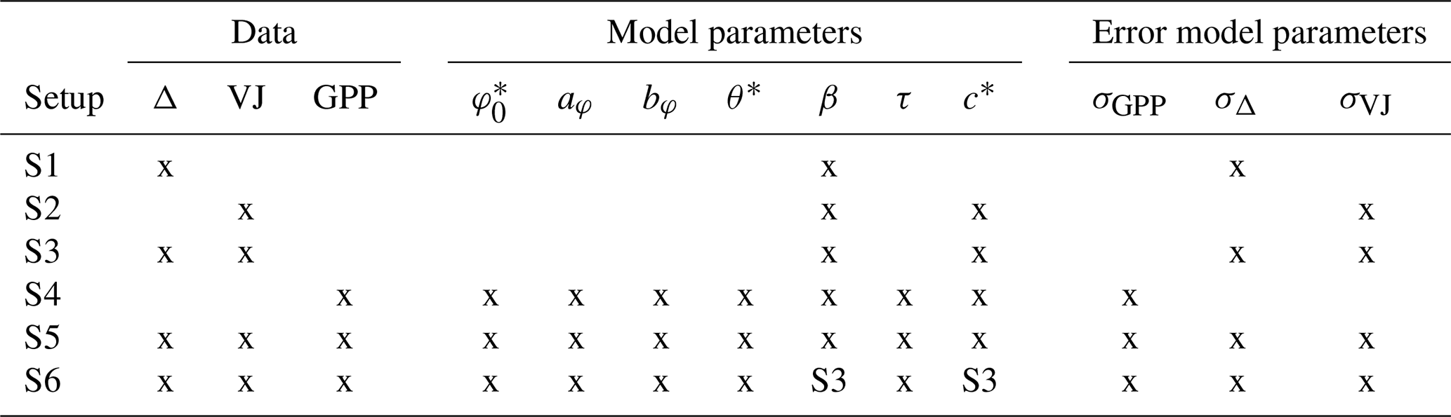
Table 2 Model parameters, their descriptions, and estimated values from different setups. Values refer to the Maximum A Posteriori (MAP) estimates. Values in square brackets represent the lower and upper bounds of uniform prior distributions or truncated normal prior distributions. 𝒩 represents a normal distribution with its mean and variance in parenthesis. Parameters that were held fixed are shown as empty cells.

^a Truncated to [0.0, 40.0]. ^b  Truncated to [187.5 to 228.2].

The choice of calibration setups was guided by our expectation of constraints on different model parameters, provided by the different target data types, given the model structure. Using common priors across (most) setups, the resulting parameter estimates can illustrate the constraints imposed by data alone. Setup S1 is chosen in view of the expected constraint of Δ data on model parameter β, Setup S2 for the expected constraint of VJ data on model parameters β and c^*, Setup S3 for these data combined constraint on both parameters simultaneously. Setup S4 analyses the constraint of GPP data on all model parameters simultaneously. Setup S5 analyses the constraint of using all three data types on all model parameters simultaneously. Setup S6 reduces the “freedom” of Setup S5 in that the posteriors from Setup 3 for β and c^* were used as priors. This corresponds to a stepwise approach and was chosen in view of results obtained for Setup S5.

We use the implementation of P-model in the rsofun R package (Stocker et al., 2025) to model daily gross primary productivity, GPP, and leaf-level traits, namely the ratio of the rates of photosynthetic capacities in the FvCB model, VJ, and the isotopic fractionation of assimilated carbon, Δ. Implementation details of the rsofun framework are provided in Appendix B.

Three latent (not directly observable) parameters govern the optimality-guided water-carbon trade-off: the unit cost ratio, β, (governing the balancing of maintaining the carboxylation capacity versus the transpiration stream), the marginal cost of maintaining the electron transport rate, c^*, and the quantum yield efficiency φ₀ (parametrized with ${\mathit{\phi }}_{\mathrm{0}}^{*}$, a_φ, b_φ).

The parameters τ, β, c^* have previously been calibrated separately to data and have been been specified as fixed model parameters in the P-model (Stocker et al., 2020; Wang et al., 2017). Here they were instead calibrated simultaneously to multiple calibration targets, together with additional parameters.

For simplicity, the same θ^*, the soil water volume (mm) below which plants are stressed, was used across all sites.

Three different calibration targets were used in this study. Δ represents accumulated assimilates and is influenced by stomatal opening through the leaf-internal to ambient carbon dioxide ratio. Equation (2) indicates its dependency on the parameter β. VJ is assumed constant throughout the season. Observations of this ratio (Eqs. 5 and 10) are expected to inform the model parameters β and c^*. GPP(t) observations represent daily values of ecosystem-level photosynthetic CO₂ uptake fluxes (with acclimation of LUE(t)). Equations (3)–(12) illustrate the dependence of these observations to model parameters β, c^*, as well as θ^*, τ, ${\mathit{\phi }}_{\mathrm{0}}^{*}$, a_φ, and b_φ.

Note that V_cmax and J_max both scale nearly linearly with φ₀ (Eqs. 5 and 10). This dependency to φ₀ mostly cancels out when considering the ratio of the two VJ.

2.3 Calibration target and test data

The data set consisted of 50 sites with GPP flux time series (172 055 site-dates in total), 49 sites with a total of 597 individual VJ observations (multiple individual plants and/or species per site sampled), and 325 sites with a total of 2357 Δ observations. Data for all variables were split by sites for model calibration (training) and out-of-sample testing (Fig. 2 and listed in Table S2). The split into training and test data sets was performed in a stratified manner according to vegetation type and land cover class (Beck et al., 2018; Copernicus Climate Change Service, 2019; Hufkens and Stocker, 2025) to ensure balanced representations of each stratum in the test and training data set. Sites, classified as croplands or wetlands were removed, as well as any site with five or less complete years of data. We additionally required that a site contained more than 12 years of good-quality gap-free GPP data to be available as a training site. We used GPP data from 12 sites for training and data from the remaining 38 sites for testing. The VJ and the Δ data were split such that data from roughly 50 % of all sites in each stratum were used for training and testing, respectively.

GPP observations were taken from FluxDataKit (FDK v3.4.2) (Hufkens and Stocker, 2025; Pastorello et al., 2020), which combines published releases of consistently processed eddy-covariance data from multiple regional networks (Ukkola, 2020; Warm Winter 2020 Team et al., 2022; Drought 2018 Team et al., 2020). GPP estimated through the nighttime flux partitioning was used (variable “GPP_NT_VUT_REF”, Reichstein et al., 2005). For model calibration and evaluation, we filtered data to retain only (daily) values that were computed with at least 80 % measured or good-quality gap-filled (half-hourly) values. Based on visual inspection, the following site-year combinations exhibited spurious patterns and were additionally removed: ES-LJu, year 2006; US-Ho2, year 2007; CH-Dav, year 2010; US-Whs years 2016 and 2017.

Observations of VJ were obtained from the data compilation of Smith et al. (2019), containing data reported for top canopy from multiple sources (De Kauwe et al., 2016; Keenan and Niinemets, 2016; Smith and Dukes, 2017; Kattge et al., 2011; Wang et al., 2018; Fürstenau Togashi et al., 2018; Togashi et al., 2018; Domingues et al., 2010; Ferreira Domingues et al., 2015; Serbin et al., 2015; Tarvainen et al., 2013; Ellsworth, 2016; Rogers et al., 2017).

Observations of carbon-13 isotope discrimination in leaf material (Δ) were taken from a global data set (Cornwell et al., 2018; Cornwell, 2025), subsetting only observations that were marked as C₃ plants. We used Δ values that were derived from the isotopic signature of leaf material in relation to the atmospheric signature at the date and latitude measurements were made.

2.4 Forcing data

For simulations of GPP time series, daily meteorological measurements, obtained in parallel with GPP observations, were used as model forcing. Daily forcing data was taken from FluxDataKit (FDK v3.4.2) (Hufkens and Stocker, 2025; Pastorello et al., 2020) and was derived from half-hourly data. The required daily variables are listed in Tab. S1. We used mean daytime air temperature and vapor pressure deficit (based on half-hourly values during daylight conditions), daily minimum and maximum temperatures, daily sum of precipitation, and daily means of net radiation, atmospheric pressure and CO₂ concentration.

For predictions of the two leaf traits (Δ, VJ), the P-model was forced with average climate conditions during the growing season, derived from the global WorldClim data set (Fick and Hijmans, 2017) (comprising monthly averages of daily minimum, maximum and average temperature, vapor pressure, and solar radiation) and considering geographic positions of the sites.

The monthly WorldClim data were temporally disaggregated to daily values through polynomial interpolation (daily minimum, maximum, and average temperatures, cloud cover fraction, solar radiation, and vapor pressure). Interpolated daily maximum and minimum temperatures were then combined to an average daytime temperature using location-based day length assuming a sinusoidal temperature profile (Davis et al., 2017; Peng et al., 2023). The average daytime vapor pressure deficit (D) was derived from the average vapor pressure and daily maximum and minimum temperature.

Daily values were averaged to conditions representing the growing season. Growing season was defined as the period with daily average temperature above 0 °C. Then, daytime temperature, vapor pressure deficit D and solar radiation were averaged (mean) across all days of the growing season and used as model forcing (T, D, PAR) for a non-temporally resolved single prediction of VJ or Δ for each site. Atmospheric pressure P was derived from the ETOPO-1 digital elevation model (NOAA National Geophysical Data Center, 2009), using site positions and assuming standard atmospheric pressure. CO₂ was taken from yearly mean values from the Mauna Loa record (Keeling et al., 2017), using the corresponding observation year (or the year 2000 if observation year was unavailable).

2.5 Bayesian calibration

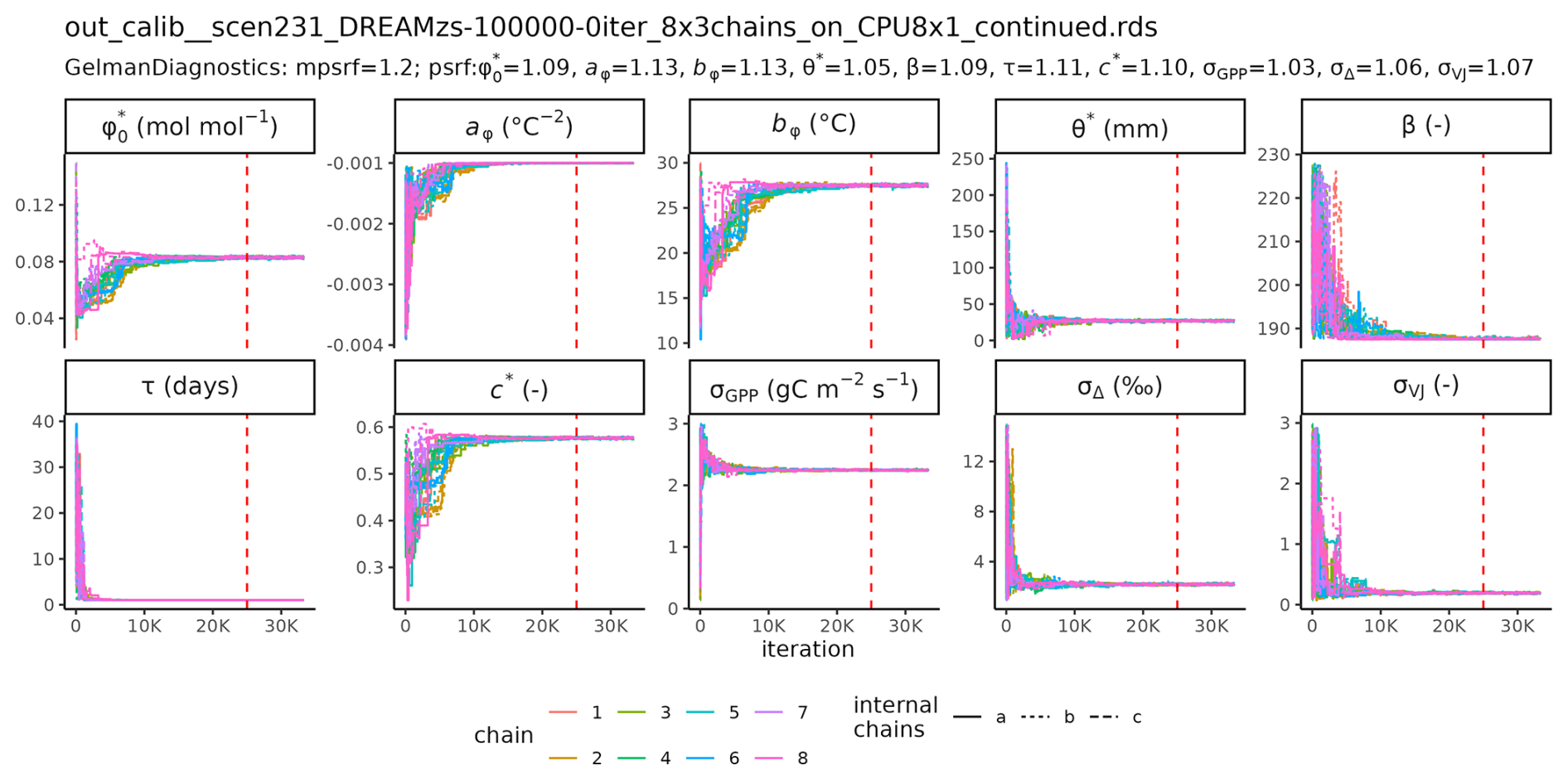
We estimated model parameters β, c^*, τ, ${\mathit{\phi }}_{\mathrm{0}}^{*}$, a_φ, b_φ, and θ^* (see Table 2 for a description of parameters) in multiple combinations of parameters and target data (Sect. 2.3 and Table 1). Parameter estimation was done through a Bayesian calibration approach, using Markov chain Monte Carlo (MCMC) sampling (Clark, 2004; Dietze et al., 2013), using the DREAMzs sampling algorithm (Vrugt et al., 2009) as implemented in BayesianTools (Hartig et al., 2023). Eight independent chains were run, each for 100 000 iterations split among three internal chains, burn-in period was set to 30 000 and convergence was checked visuall with trace plots and Gelman–Rubin statistics (Gelman and Rubin, 1992). Parameters were calibrated to all sites' data simultaneously and are thus assumed to be universal across space and environmental conditions.

2.5.1 Likelihood

The choice of likelihood summarized our assumptions about different sources of uncertainties. Uncertainties in model inputs (parameters p and forcings x), in model structure f, and in the measured observations y of all target types (van Oijen, 2017) combine as

$$y+{\mathit{\epsilon }}_y=f\left(p,x+{\mathit{\epsilon }}_x\right)+{\mathit{\epsilon }}_f$$

where ε_y and ε_f represent (unknown) observational errors and model structural errors, respectively. ε_x is the error in the forcing data.

For all target variables, we assumed an additive and normally distributed model error term around the model prediction (Trotsiuk et al., 2020) and expressed the fit to observed data via the Gaussian log-likelihood

$$\begin{array}{}\text{(16)}& {\displaystyle }\mathcal{L}(p\mid y)={\displaystyle \frac{\mathrm{1}}{\sqrt{\mathrm{2}\mathit{\pi }{\mathit{\sigma }}^{\mathrm{2}}}}}\exp \left(-{\displaystyle \frac{\mathrm{1}}{\mathrm{2}{\mathit{\sigma }}^{\mathrm{2}}}}(y-f(p,x){)}^{\mathrm{2}}\right)\end{array}$$

with target-specific standard deviations σ_GPP, σ_Δ, and σ_VJ. These standard deviations of the error model were estimated together with the model parameters (Table 2). Individual observations were considered independent from each other, thus the total likelihood for a dataset simply multiplied the likelihoods of each observation. With this likelihood, we neglected input error ε_x=0 and lumped together observational uncertainties and model structural uncertainties into a single “mismatch” or “residual” uncertainty (van Oijen, 2017; Dietze et al., 2013).

Since the P-model is conceived as a single-big-leaf model (Fig. 1), it represents average properties and fluxes for the whole canopy. The estimated residual uncertainty thus contains also a potential uncertainty due to the scale mismatch between observation and model. Moreover, across-tree and across-species variabilities are also included since the likelihood was computed for each VJ and Δ observations of individual trees.

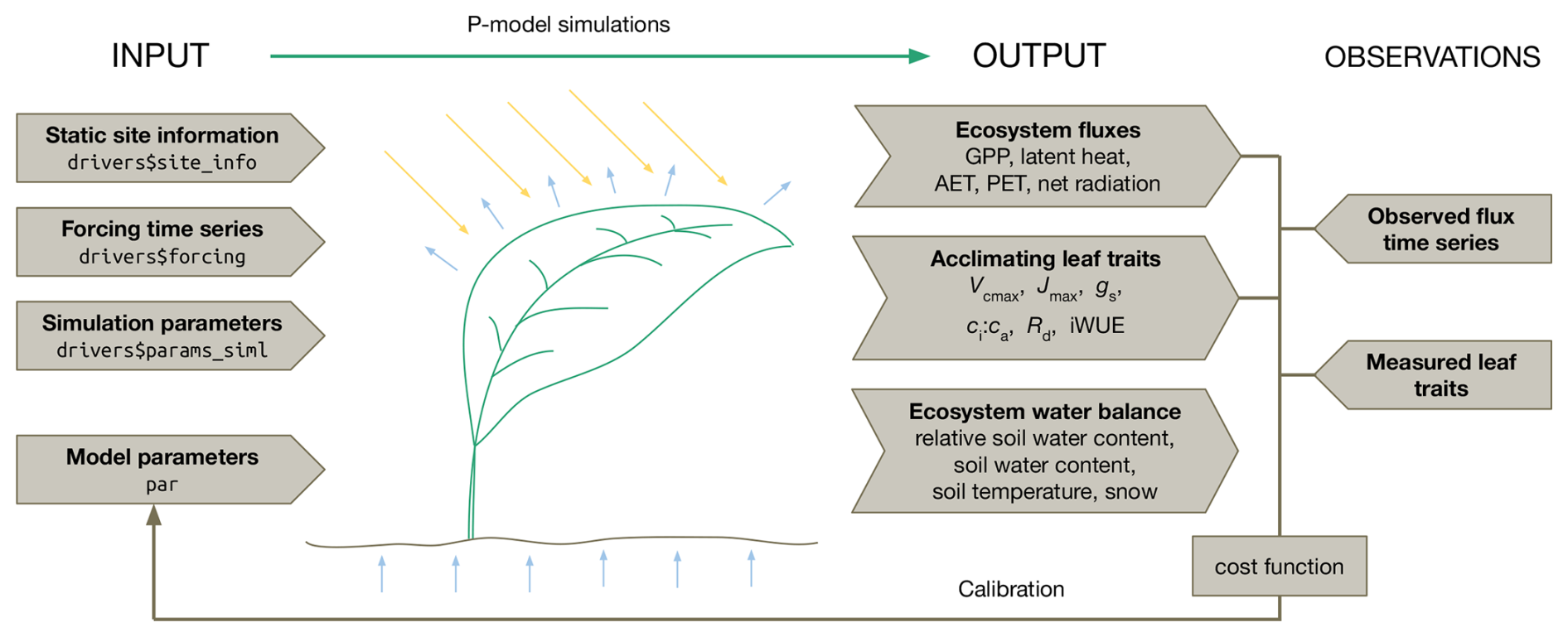
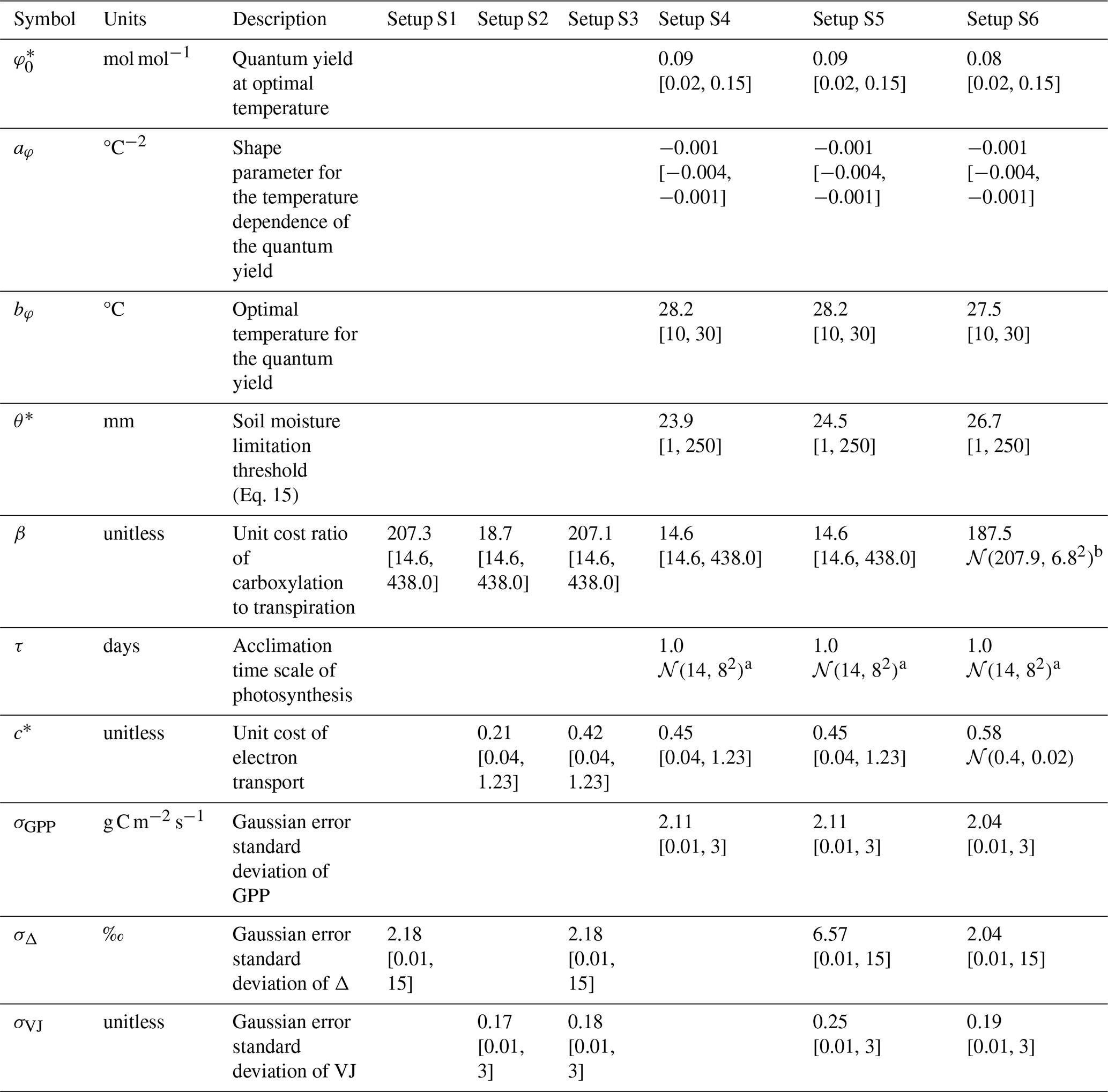
Figure 1 P-model inputs, outputs, and target observations for the parameter estimation. The model takes as inputs static site information, time series of meteorological forcings, simulation parameters, and common model parameters for all sites. The simulation returns a time series of several ecosystem fluxes, acclimating leaf traits and ecosystem states. By comparing these outputs with measured traits and flux data in a Bayesian calibration routine, model parameters can be estimated. The structure (named list) of the input data object (driver) used for the model call within the rsofun R package is given in the “arrow boxes” on the left. Variable names of predicted quantities are given in the “arrow boxes” under “output” and are described in the main text.

Figure 2 Global maps of site locations (red dots) with observations of the three target variables in the training and test data sets for (a) GPP, (b) VJ, (c) Δ.

While describing leaf-level quantities at relatively high mechanistic detail, the link between the leaf and the canopy-scale was not explicitly resolved. Instead, an empirical approach for leaf-to-canopy scaling of GPP was employed by treating the quantum yield parameter φ₀ to be representative for the canopy-scale and allowing it to be calibrated to ecosystem-level GPP flux data.

2.5.2 Priors

Prior distributions were defined based on prior knowledge and kept the same across all calibration setups, except for setup S6, where the posteriors of the model parameters β and c^* estimated from setup S3, were used as priors (Table 2 and shown in grey in Fig. 3). These posteriors from setup S3 were characterized as uni-variant normal distribution. For β, it was additionally truncated to the mean ± three times the standard deviation.

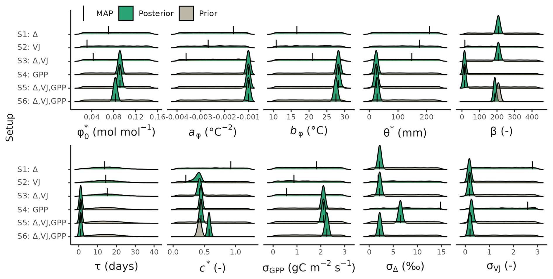
Figure 3 Prior and posterior distributions of the calibrated model parameters and error model terms for different setups. The maximum a posteriori (MAP) estimates are indicated with a solid line. See Table 2 for parameter descriptions.

The prior knowledge on the acclimation time scale τ was approximated by a normal distribution (with mean and variance of 𝒩(14, 8²)) based on prior findings (Mäkelä et al., 2004; Liu et al., 2024; Mengoli et al., 2022) and truncated to the range from 0 to 40 d. For all other parameters, uniform priors with distinct ranges were used. Ranges for β, c^*, and ${\mathit{\phi }}_{\mathrm{0}}^{*}$ were specified to range between 10 % and 300 % of published estimates of 146 (unitless), 0.41 (unitless), and 0.05 mol mol⁻¹, respectively, (Stocker et al., 2020; Wang et al., 2017). We chose wide uniform priors with the aim that posteriors would solely be informed by the used observations. The optimal temperature b_φ and shape parameter a_φ were specified to range between 10 and 30 °C and −0.004 and −0.001 °C⁻². The soil moisture limitation threshold θ^* was specified to range between 1 and 250 mm. Given the lack of prior knowledge on the error parameters characterizing the combined structural and observational uncertainty large, uninformative priors were assumed.

2.6 Prediction uncertainty

The parameter sets generated by the MCMC chains provide the basis for model prediction including an estimation of the uncertainty in the predictions on the train and test data set. Here, we propagated both characterized uncertainties: the parametric and the residual (structural and observational) uncertainty.

Retaining 20 samples from the combined Markov chains, representative of the joint parameter posterior distribution (including parameter correlations), we ran the P-model for each set of parameters to predict the target variables for the test and training data set. These 20 sets of predictions represented the parametric uncertainty of the model.

Additionally, for each prediction (i.e. target, site, and date combination) three observational errors were drawn from the residual error model (characterized by σ_GPP, σ_Δ, and σ_VJ) and added to the prediction. These 60 sets of predictions represented the combined parametric and residual uncertainty of the model. These samplings appeared sufficient, since results did not change upon sampling 50×10 parameter/error pairs. A third comparison with observations was based on one set of predictions using the Maximum A Posteriori estimate as a single set of parameters and without considering the residual uncertainty.

3 Results

3.1 Calibrated parameters

MCMC sampling with DREAMzs of 8 parallel, independent chains took between 2.5 h (S2) and 68 h (S6) to reach 100 000 iterations for the setups S1 to S6. The trace plot of the chain of setup S6, including computations of the scale reduction factors (Gelman and Rubin, 1992) are reported in the Appendix (Fig. C1).

Posterior distributions of the estimated parameters varied across the different setups (Fig. 3). Setup S1 (using only Δ as observational target) constrained β to a maximum a posteriori (MAP) of 207 (unitless), a median of 208 and with an inter-quartile range (IQR) from 203 to 213 and the residual prediction error σ_Δ to a MAP of 2.18 (unitless), which corresponds to a 10 % of the mean of predicted Δ. Other parameters were not informed by the calibration and their posteriors remained largely identical to their prior distributions. This reflects model structural dependencies of parameters and predicted quantities (Δ is independent of the other model parameters, see Eq. 3).

Setup S2 (using only VJ as observational target) constrained c^* to a MAP of 0.214 (unitless), (median of 0.397, IQR from 0.347 to 0.428). As revealed by the posterior correlation analysis, β and c^∗ showed a strong correlation (r=0.86, Fig. C2). These compensating effects were disentangled when simultaneously calibrating to Δ and VJ in setup S3. This constrained β to a MAP of 207.1 (unitless), (median of 207.9, IQR from 203.5 to 212.3) and c^* to MAP of 0.419 (unitless) (median of 0.425, IQR from 0.410 to 0.439), slightly higher than in setup S2, and avoided the correlation of posteriors (Figs. 3 and C3). The error model parameters associated with the two targets Δ and VJ were estimated to MAPs of 2.18 ‰ and 0.178 (unitless).

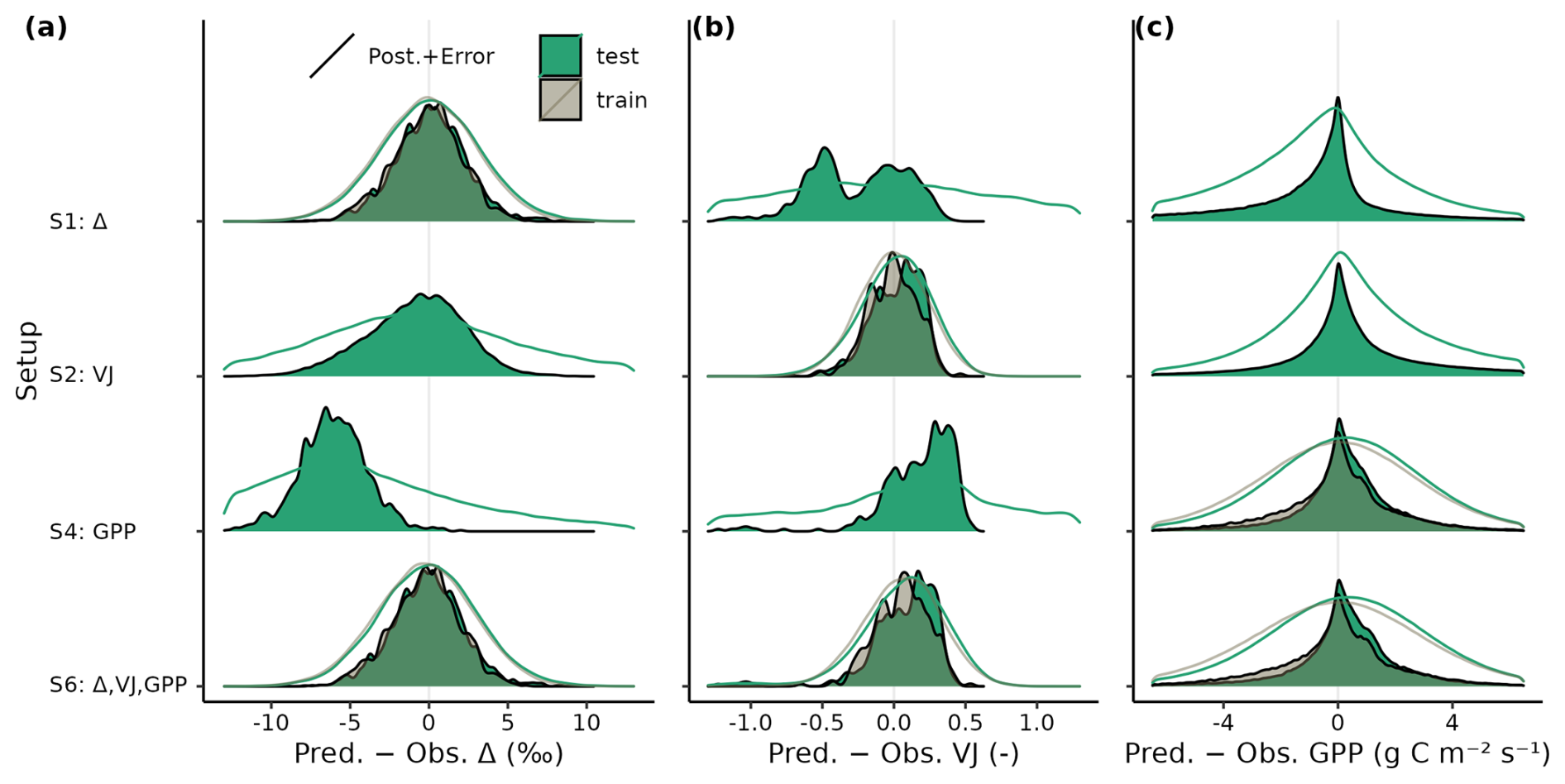
Figure 4 Density plot of residuals between predicted and observed (a) Δ, (b) VJ and (c) GPP from the training (grey) and test sets (green) for calibration setups S1, S2, S4, and S6. Model output is computed with parametric uncertainty (filled area, based on 20 samples from the posterior distribution) and residual uncertainty (solid line, based on 3 samples from error model). Model outputs are compared against individual observations (dates from all sites pooled for GPP, and individual observations of each site for Δ and VJ).

Setups that use GPP as observational target and uninformed priors – setups S4, and S5 – yield estimates of β that are at the lower bound of the uniform prior range – i.e. 14.6 (unitless) –, while τ is estimated to be exactly 1 d. This indicates that GPP observations “push” estimates of β towards extremely high unit costs of transpiration in relation to carboxylation, and that no smoothing of the daily meteorological conditions (Eq. A1) was necessary to optimize the likelihood of observing the GPP data. However, while improving the likelihood of GPP, the fit with Δ observations was deteriorated in these setups, as indicated by an offset between model predictions and observations (Figs. 4 and 5). Only setup S6, using GPP in combination with a truncated and prior for β, informed by the reduced setup S3, mitigates this offset. Also here, the posterior estimate of β came to lie at the border of the truncated region – 14.6 (unitless). The error model parameter associated with the GPP target was estimated to a MAP of 2.04 g C m⁻² s⁻¹ in setup S6, which was slightly smaller than the error in setups S4 and S5. In the posterior parameters of setup S6, correlations of r=0.89 remain between ${\mathit{\phi }}_{\mathrm{0}}^{*}$ and c^* and of r=0.81 between φ₀ and b_φ (Fig. C4).

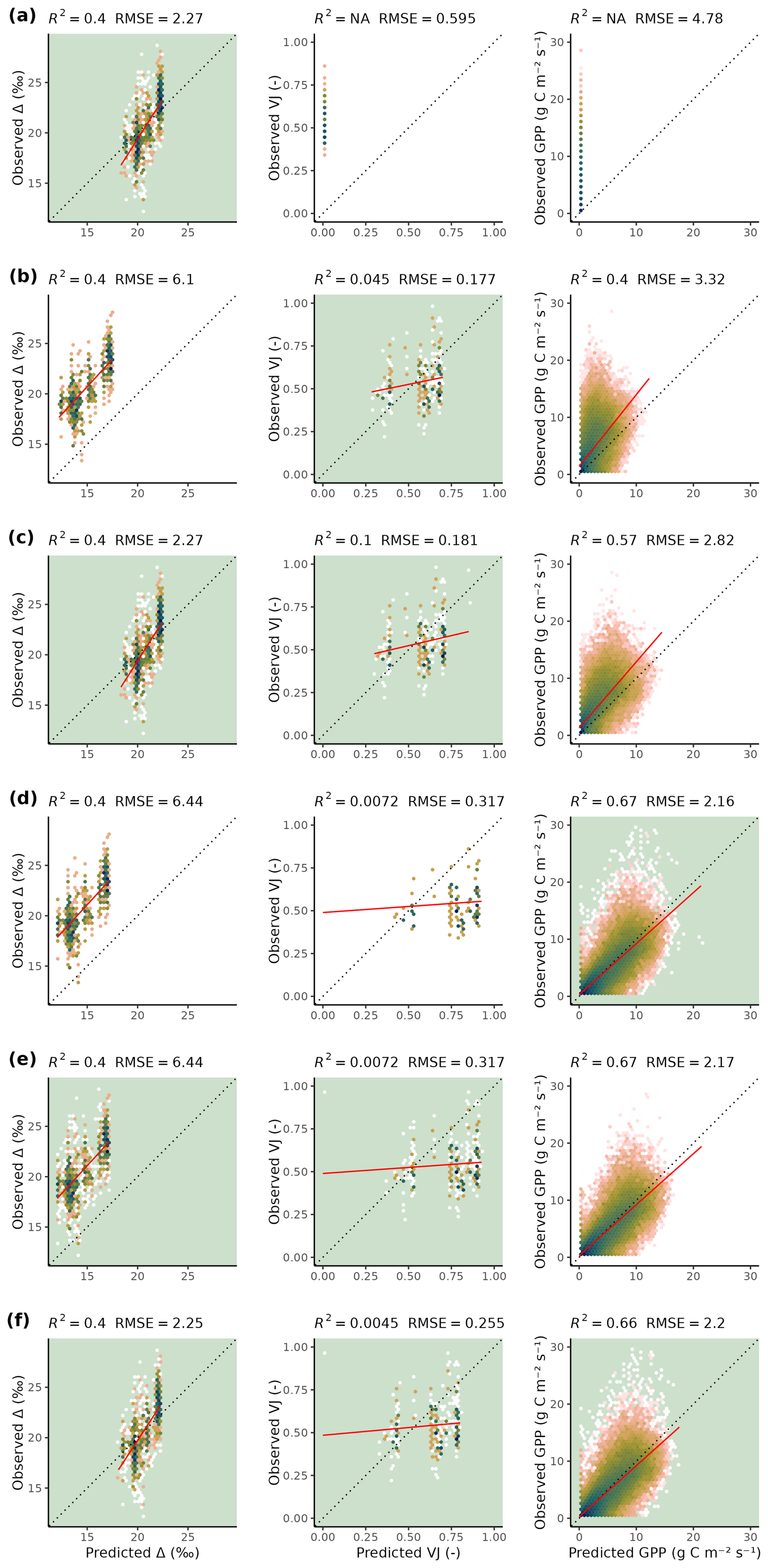
Figure 5 Predicted versus observed values for different target variables (Δ, VJ, and GPP along columns) and calibration setups (S1, S2, S3, S4, S5, and S6, along rows), evaluated on the test set. Model output is computed with Maximum A Posteriori parameter values (MAP) for each calibration setup. Note that the MAP parameters from setup S1 result in null-predictions of VJ and GPP. Color indicates density, red line indicates a linear regression. Green panel backgrounds indicate which variables were used as targets for model calibration in the corresponding setup. Model outputs are compared against individual observations (predicted and observed daily GPP values from all sites pooled and site-specific predictions against all observations from the respective site for Δ and VJ).

3.2 Prediction uncertainty

Model predictions were unbiased and residuals were of similar magnitude when evaluated on the test and on the training data sets (Fig. 4), which indicates a good generalizability of the parametrized model. Including structural and observational uncertainties on top of parametric uncertainties only slightly increased the deviations between predicted and observed targets in setup S6, with strongest relative increases for GPP.

Δ and GPP predictions based on MAP parameter sets of setup S6 showed no magnitude-dependent bias (linear slopes of regressions between predicted and observed values were close to 1), whereas VJ showed a prediction range that appears too large when compared to the observed range (slope close to 0, Fig. 5). Setup S6 showed a slightly worse root mean squared error (RMSE) than setup S5 for GPP, but clearly reduced RMSE for Δ and VJ.

Time series of GPP of a few select years on training site data showed that the model successfully reproduced seasonal patterns and differences across site in GPP for most sites (Fig. C5), with some shortcomings in accurate simulations of GPP during under dry conditions, as seen for site US-Var, and a general low bias for the moist tropical site of GF-Guy. The model also tends to systematically overestimate GPP in the early growing season at US-MMS and US-PFa – a known bias (Luo et al., 2023).

4 Discussion

This study showed that a model for ecosystem photosynthesis and its acclimation to the environment can be robustly parameterised and that its predictions of multiple variables generalise well across a wide range of environmental conditions. Multiple model parameters can be estimated simultaneously by using diverse calibration target data types, combining ecosystem flux time series and static, species-specific traits data. This demonstrates how the explicit representation of connections between traits and process rates enable model-data integration on the basis of diverse observations, obtained at multiple organisational levels – from the leaf to the canopy. The robustness of the parameter estimates is indicated by the convergence of the MCMC chains (Fig. C1) and the resulting narrow posterior distributions of Bayesian parameter estimates (Fig. 3). Despite being calibrated to only a relatively small set of sites with GPP data (N=12), the calibrated model generalizes well, as validated against an independent and much larger set of test data for GPP from 38 sites (Figs. 4 and 5).

Our results confirmed the expectation that the use of multiple observational targets yields more robust parameter estimates compared to a calibration setup that relies on a single data source, and that specific observation types imposed constraints for specific model parameters. Leaf carbon fractionation observations, Δ, allowed to constrain the unit cost ratio of carboxylation to transpiration, β (Fig. 3). Observed ratios of the biochemical rates of carboxylation to electron transport, VJ, constrained β and c^*, albeit with strong correlations between them, indicating compensating effects and a lack of robustness in resulting parameter estimates (Figs. 3 and C2). The combination of both these observation types allowed to constrain both parameters simultaneously, avoiding correlations between parameter estimates. This indicates that the use of two observational targets simultaneously made use of their complementary information content for parameter estimation in our model (Fig. C3).

Despite the general robustness of parameter estimates, we found several limitations and aspects that indicate challenges for model calibration in our case. When observations of GPP were included in calibration setups, parameter estimates of β differed strongly from results obtained from setups that used only observations of Δ and tended towards the lower margin of the uniform prior range – substantially lower than the value used for direct parameterisation of the model in previous work (Wang et al., 2017). β represents the ratio between the unit cost of carboxylation to transpiration within the EEO modelling framework applied here (Prentice et al., 2014). An extremely low value of β implies relatively high costs associated with transpiration, which is driven by vapor pressure deficit D. The calibration tending towards low values of β potentially reflects a compensating effect for the lack of GPP reductions under conditions of dry soils, e.g., during the dry summer periods at the site US-Var (Fig. C5). In other words, this apparent lack of robustness of parameter estimate may indicate a misspecification of the model structure. This interpretation could be tested with targeted setups (e.g., removing dry sites from the calibration data set) or by alternative specifications of the soil moisture stress that better accounts for its limiting effect on GPP.

To address this challenge and avoid unexpectedly low estimates of the unit cost ratio parameter β, we resorted to a step-wise Bayesian calibration (MacBean et al., 2016) and used the posterior distribution of setup S3 as a prior in setup S6. This resulted in the disappearance of offsets in Δ observation, a c^* closer to, but not at, the upper limit of the prior (MAP = 0.58), and a sightly lower ${\mathit{\phi }}_{\mathrm{0}}^{*}$ than in GPP-only setup (S4) or in the unconstrained GPP-Δ-VJ setup (S5). The step-wise posterior estimation and prior specification of P-model parameters in setup S6 yielded estimates of all parameters that compared favourably with previous estimates (Stocker et al., 2020; Wang et al., 2017). This study estimated (MAP): β=208 (unitless, compared with 146 and the range from 200 to 240), $c*=\mathrm{0.58}$ (unitless, compared with 0.41), and ${\mathit{\phi }}_{\mathrm{0}}^{*}=\mathrm{0.05}$ mol mol⁻¹ (compared to 0.05). However, the MAP estimate of τ=1, indicated an instantaneous acclimation appeared to yield better agreement of model output with daily GPP observations, than a delayed acclimation using smoothed versions of the environmental conditions. This contrasts with previous estimations of the acclimation time scale being on the order of 14 to 15 d (Mäkelä et al., 2004; Liu et al., 2024; Mengoli et al., 2022).

Remaining correlations in posterior parameters of setup S6 between ${\mathit{\phi }}_{\mathrm{0}}^{*}$ and c^* indicate some equifinality. These compensating effects indicate another potential implicit “misinterpretation” of what the parameter c^* represents in setup S2 versus setup S6, and/or model structural error and inaccurate process representation. The Bayesian approach allows propagating the effect of this into predictive uncertainties by using posterior distributions instead of point-estimates of parameters. Still, this entanglement might be resolved in future calibrations by fixing one of these two parameters or by using additional observations. Future work is needed to look into causes of this posterior variability of c^*, identify potential observational constraints, and potentially to revise related model structures.

The calibrated model of setup S6 showed unbiased predictions against observations in an independent test data set, indicating the model's generalizability. Based on the universal validity of the EEO parameters across plant functional types and biomes, the calibrated P-model can may be scaled to new locations sites and environmental conditions. However, it should be noted that our estimates of prediction uncertainty and the finding of robust generalisability only applies to environmental conditions that are within the domain of (or similarly distanced to) sites used for training and testing here (Ludwig et al., 2023). Further caveats apply. The choice of the specification of soil moisture stress, which uses a single global parameter θ^*, may be overly simplistic for describing diverse physiological responses to dry-downs across sites characterised by different soil texture (Fu et al., 2022; Wankmüller et al., 2024) and the model neglects the highly variable rooting zone water storage capacities across space globally (Stocker et al., 2023). Although generalization to the test data set did globally show unbiased predictions across all sites (Fig. 4), shortcomings were visible for certain sites (e.g., US-Var, Fig. 5) and warrant a re-consideration and potential revision of the related process representations. An improved representation of soil moisture stress effects and across-site variations of critical soil moisture thresholds and storage capacities may potentially also mitigate the need for targeted interventions into the calibration procedure, e.g., through the truncation of the prior for β or the step-wise approach to model calibration. More specifically, θ^* could potentially be expressed by additionally considering soil structural information (Wankmüller et al., 2024), which could be provided as additional information for each site. Alternatively, the Bayesian approach allows for the use of hierarchical models (van Oijen, 2017) that could make use of potential, globally available predictors (or covariates) for the site-specific parameters.

Generally, design choices related to the Bayesian likelihood specification and parameter calibration were adequate to showcase the sensitivity of parameter estimates across setups and retrieve an unbiased, generalizable model. While simple, the additive Gaussian error model chosen for the likelihood was sufficient to illustrate the constraints. However, more appropriate functional forms could be used – for example, ones that account for the fact that GPP values should be non-negative and that observational errors tend to scale with the magnitude of the flux (Cameron et al., 2022), or that better separate observation uncertainty from model structural uncertainty (van Oijen, 2017). Independent estimates of observation uncertainty could be included as fixed parameters or as informed priors. This would potentially lead to a reduced residual error representing more closely the structural model uncertainty. Potential estimates for these could be the error on GPP measurements or errors of a trait measurement to represent the model scale (i.e. the ecosystem-level averages across species instead of individual observations). Alternatively, fitting to average observations instead of individual observations might reduce the (independent) observational errors. This would mean fitting to averaged traits over different species at a given site or weekly cumulative fluxes instead of daily values.

A strength of the Bayesian approach is to update model parameters iteratively with additional data by using previous posteriors as new prior distributions. Our illustration of this approach in setup S6 relied on manual extraction and specification of these distributions. A future development step for the rsofun framework would thus be to support easier specifications of these type of stepwise calibration (MacBean et al., 2016) directly through the model interface.

The model employed here, the P-model, describes light absorption, utilisation, and CO₂ uptake at an aggregated organisational scale – the canopy-level. Despite this simplified representation, we found that parameter interactions and structural model errors can to lead biases in parameter estimates. The stepwise calibration approach allowed to rectify (likely biased) estimates of β that deviated from estimates used in previous work (Prentice et al., 2014; Wang et al., 2017; Stocker et al., 2020). This violated the initial aim of simultaneously estimating all parameters, but is interpreted here as an indication of where to find structural deficiencies and target model improvements (Oberpriller et al., 2021). More comprehensive vegetation models of larger scope, e.g., Dynamic Global Vegetation Models (Sitch et al., 2024), will likely face similar challenges, considering that structural deficiencies are unavoidable and more parameter interactions may arise through feedbacks in the soil-plant system. Our findings indicate that stepwise approaches to model calibration can be a solution to this challenge.

While this study looked at seven model parameters simultaneously, several other parameters were held fixed, namely those involved in describing temperature and pressure dependencies of physical and physiological quantities, isotope fractionation, etc. This simplified the calibration and parameter estimation task, but assumed that the uncertainty stemming from these is negligible for the prediction of target variables. This is a strong assumption and may be relaxed in future attempts at calibrating P-model.

Lastly, the chosen likelihood ignored input data uncertainty ε_x. For sites from which GPP estimates were obtained, we expect small uncertainty in meteorological variables thanks to local measurements. In contrast, fAPAR data is obtained from satellite remote sensing data, which is likely to include uncertainties. For sites from which Δ and VJ data was obtained, input forcing was based on a global dataset of high spatial resolution (∼1 km around the equator). However, topographical effects and related micro-climata that deviate from the larger climate could be remaining sources of errors.

The rsofun R package provides a user-friendly and efficient implementation of the P-model and off-the-shelf model-data assimilation functionalities through its connection to the BayesianTools R package (Hartig et al., 2023), while maintaining flexibility for altered calibration setups and likelihood definitions. P-model's computational efficiency offered the potential for effective model parameter and uncertainty estimation using Bayesian statistical methods in combination with flux and traits data here.

Our model implementation as an R package takes inspiration from the r3PG forest model (Trotsiuk et al., 2020), and our implementation of model-data integration on the basis of ecosystem data serves similar, yet reduced aims and functionalities compared to PEcAn (https://pecanproject.github.io/index.html, last access: 25 November 2025) (LeBauer et al., 2013). rsofun is designed to be minimally reliant on package dependencies and connections to specific data, while limiting the scope to a predefined set of process models (currently P-model, BiomeE at an experimentation stage). rsofun and the implementation of our simulations and analyses shown here in accompanying code (see code availability statement) and package vignettes provide a blueprint for model-data assimilation for modelling terrestrial photosynthesis.

5 Conclusions

This study used rsofun (available as an R package) to calibrate latent P-model parameters to a set of flux and traits data, obtained from 193 training sites and 231 test sites. Predictions across all test sites showed that the calibrated model generalized well, not showing any biases and similar prediction residuals between train and test data. The Bayesian calibration also exhibited challenges. Structural uncertainty, the imbalanced data set, and a potentially too simplistic likelihood lead to biased parameter estimates and predictions in the first calibration attempt. An alternative calibration setup made use of a stepwise calibration and the hierarchical design of the model structure and predictions, enabling a successive model integration and parameter calibration. The necessity for this approach to obtain robust and reliable parameter estimations may indicate model structural deficiencies, which we identified here as primarily being related to the representation of effects by dryness in soil and air.

Appendix A: Acclimation

Damped acclimation to daily environmental conditions was considered for the GPP prediction, while for Δ and VJ predictions used growing season average conditions.

The the low-pass filter of characteristic time scale τ (days) is defined as

$$\begin{array}{}\text{(A1)}& \begin{array}{rl}T(t+\mathrm{1})=& T\left(t\right)+{\displaystyle \frac{\mathrm{1}}{\mathit{\tau }}}\left(T^{\prime }\right(t+\mathrm{1})-T(t\left)\right),\\ & \mathrm{initialized}\mathrm{as}T\left(\mathrm{0}\right)=T^{\prime }\left(\mathrm{0}\right),\end{array}\end{array}$$

where T is the low-pass filtered quantity (here temperature) and T^′ the daily observations, resulting in a daily time series of the damped quantity. Equivalent expressions with the same τ are used for P, D, CO₂, and PAR.

Appendix B: The rsofun model framework

rsofun implements the P-model (Stocker et al., 2020) and provides off-the-shelf methods for Bayesian (probabilistic) parameter and prediction uncertainty estimation. rsofun is distributed as an R package on R's central and public package repository. rsofun also implements the BiomeE vegetation demography model (Weng et al., 2017, 2015). The latter is not further described here and is implemented at an experimental stage in rsofun version v5.1. The P-model implementation in rsofun is designed for time series simulations by accounting for temporal dependencies in the acclimation to a continuously varying environment. Function wrappers in R make the simulation workflow user-friendly and all functions and input forcing data structures are comprehensively documented (https://geco-bern.github.io/rsofun, last access: 25 November 2025).

In rsofun, model parameters can be calibrated using a calibration function calib_sofun( ), providing two modes of calibration, one based on generalised simulated annealing (GenSA R package) for global optimization (Xiang et al., 2013) and one based on Markov chain Monte Carlo (MCMC) implemented by the BayesianTools R package, giving access to a wide variety of Bayesian methods (Hartig et al., 2023). The former being fast, while the latter provides more informed parameter optimization statistics (Clark, 2004; Dietze et al., 2013). This gives the option for both exploratory and more in-depth analysis of estimated parameters. A set of standard cost functions are provided for the calibration, facilitating the exploration of various metrics or target variables and the specification of calibrated model parameters. Furthermore, the vignettes accompanying the package (https://geco-bern.github.io/rsofun/articles/, last access: 25 November 2025) explain how to customise the calibration cost functions and interpret the calibration results.

Appendix C: Posterior parameter estimates

C1 Posterior parameter sampling

Figure C1 Trace plot of MCMC sampling of all parameters in setup S6.

C2 Posterior parameter correlations

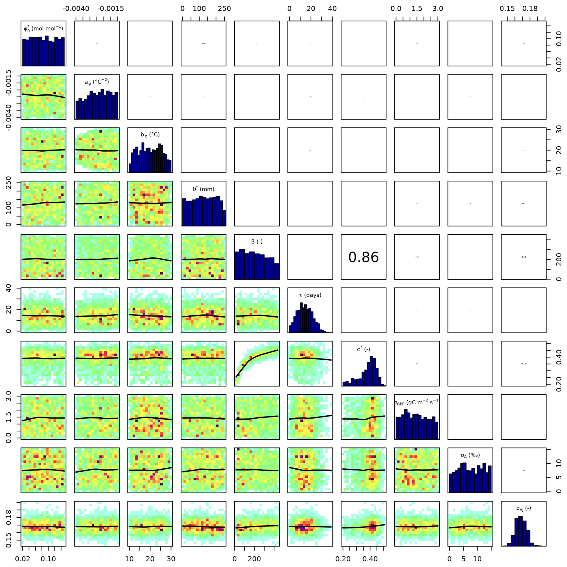
Figure C2 Parameter correlation of posterior parameters in setup S2 with 100 000 iterations and 30 000 burn-in.

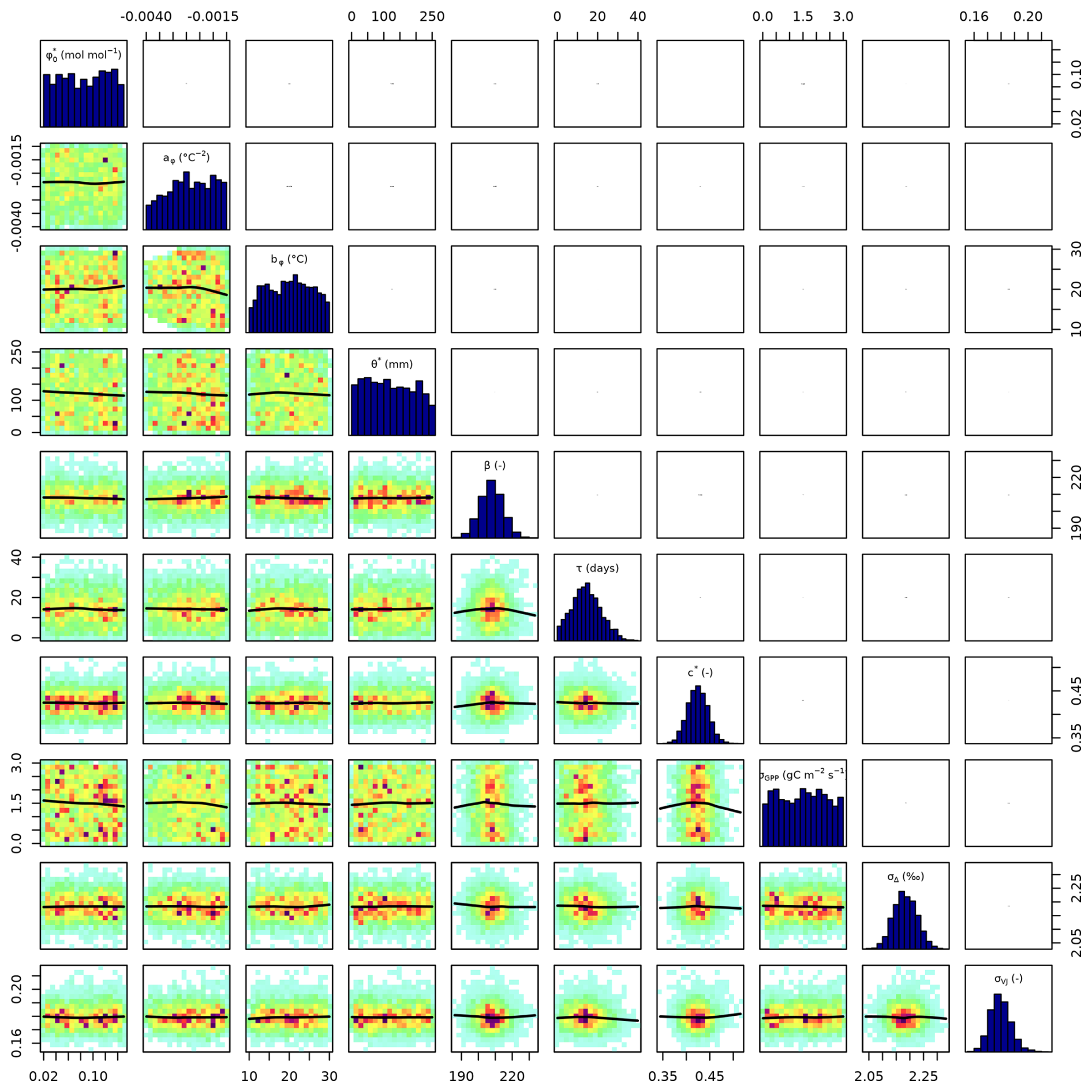
Figure C3 Parameter correlation of posterior parameters in setup S3 with 100 000 iterations and 30 000 burn-in.

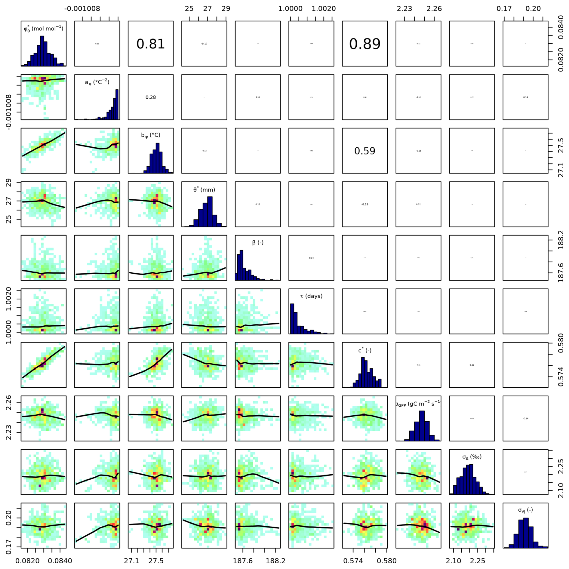
Figure C4 Parameter correlation of posterior parameters in setup S6 with 100 000 iterations and 30 000 burn-in.

C3 Posterior parameter predictions

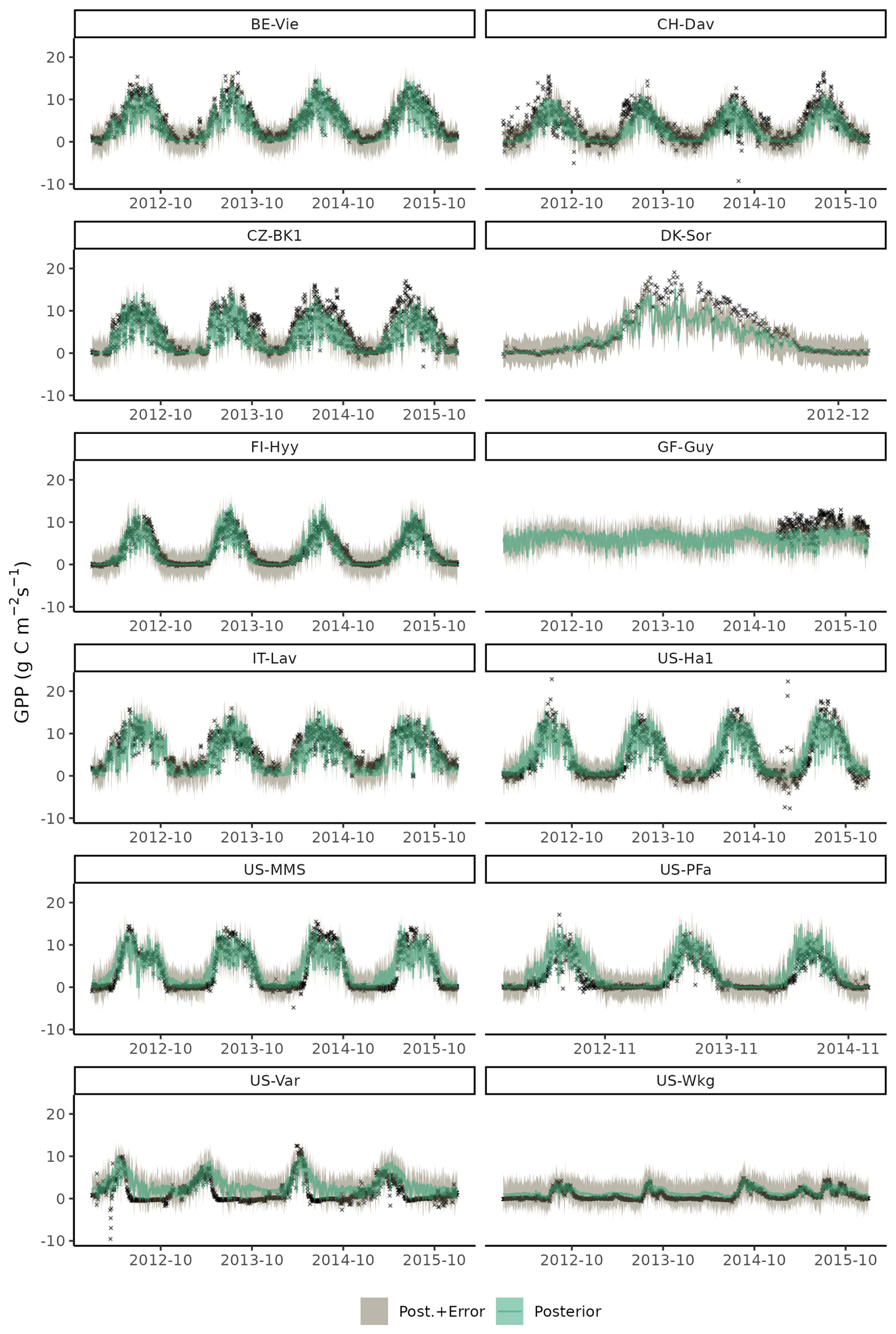
Figure C5 Time series plot of observed (black crosses) and modelled daily gross primary production (GPP) for setup S6 for years 2012 to 2015 of the training data set. Model output is computed with parametric uncertainty (green shaded area, based on 20 samples from the posterior) and structural uncertainty (grey shaded area, based on 3 samples from error model).