A new metrics framework for quantifying and intercomparing atmospheric rivers in observations, reanalyses, and climate models

We present a new atmospheric river (AR) analysis and benchmarking tool, namely Atmospheric River Metrics Package (ARMP). It includes a suite of new AR metrics that are designed for quick analysis of AR characteristics via statistics in gridded climate datasets such as model output and reanalysis. This package can be used for climate model evaluation in comparison with reanalysis and observational products. Integrated metrics such as mean bias and spatial pattern correlation are efficient for diagnosing systematic AR biases in climate models. For example, the package identifies the fact that, in CMIP5 and CMIP6 (Coupled Model Intercomparison Project Phases 5 and 6) models, AR tracks in the South Atlantic are positioned farther poleward compared to ERA5 reanalysis, while in the South Pacific, tracks are generally biased towards the Equator. For the landfalling AR peak season, we find that most climate models simulate a completely opposite seasonal cycle over western Africa. This tool can also be used for identifying and characterizing structural differences among different AR detectors (ARDTs). For example, ARs detected with the Mundhenk algorithm exhibit systematically larger size, width, and length compared to the TempestExtremes (TE) method. The AR metrics developed from this work can be routinely applied for model benchmarking and during the development cycle to trace performance evolution across model versions or generations and set objective targets for the improvement of models. They can also be used by operational centers to perform near-real-time climate and extreme event impact assessments as part of their forecast cycle.

1 Introduction

Atmospheric rivers (ARs) are dynamically driven synoptic-scale filamentary structures of water vapor jets that play important roles in the global water cycle and regional weather and hydrology (Ralph et al., 2013; Gimeno et al., 2014; Shields et al. 2019; Payne et al. 2020; O'Brien et al., 2022). These narrow, concentrated corridors of moisture in the atmosphere can carry an immense amount of water, often compared to the flow of multiple major rivers combined (Ralph and Dettinger, 2011), and account for more than 90 % of extratropical poleward water vapor transport (Zhu and Newell, 1998; Newman et al., 2012; Ullrich et al., 2021). When making landfall or interacting with topography, ARs can produce extreme weather, including heavy rainfall and strong winds, in turn leading to severe flooding and landslides. These effects can devastate natural landscapes, agricultural fields, and human infrastructure and disrupt businesses and services, leading to significant economic losses (Ralph et al., 2006; Leung and Qian, 2009; Neiman et al., 2011; Neiman et al., 2013; Gershunov et al., 2019). However, ARs are also essential for delivering water for agriculture, ecosystems, and human consumption; in the western United States alone they are responsible for one-third to one-half of total annual precipitation (Ralph and Dettinger, 2011).

Because ARs can be responsible for both beneficial and detrimental impacts, understanding and modeling of these features, particularly in light of climate change, constitute an important topic. To date, however, proposed definitions of ARs have yet to be widely adopted (Ralph et al., 2018), which has in turn made it difficult to draw conclusions about how these features may be changing. Numerical algorithms for objective identification of ARs, namely AR detectors (ARDTs) (e.g., Neiman et al., 2009; Dettinger et al., 2011; Ralph et al., 2013; Mundhenk et al., 2016; Ullrich and Zarzycki, 2017; Ullrich et al., 2021), have widely facilitated broader studies of AR characteristics and impacts (Shields et al., 2019b; Rutz et al., 2019; O'Brien et al., 2022). However, as ARDTs are usually designed with particular research questions in mind, the lack of a unified framework that is applicable to different ARDTs in a collective way has challenged the benchmarking and intercomparison of the models' representation of ARs. The analysis workflow and code in one study cannot be easily applied in another study using a different ARDT. Consequently, studies like intercomparison of ARDTs or analysis based on an ensemble of ARDTs cannot be readily executed without extensive collaboration or community efforts. In addition, research of this kind cannot be easily repeated or updated when newer versions of ARDTs have been developed or newer observational data products have become available. As such, a universal analysis framework that is independent of ARDT is in demand in our AR research community.

Within AR research, one major branch focuses on evaluating the performance of forecast or climate models in simulating ARs. Since the number of climate models under active development and used in the research community has increased substantially in recent decades, with many supporting multiple configurations and parameterization choices, routine evaluation of ARs during model development life cycles requires a quantitative climate data assessment evaluation workflow that allows comparing AR characteristics from different ARDTs. We believe progress in improving our understanding of ARs and their impacts could be accelerated with a dedicated tool for calculating AR statistics and evaluation metrics in climate models and gridded data products. Preferably, such an analysis tool should be seamlessly applicable to multiple data sources (including observations, forecast, reanalysis, and different models) with simply a few commands, minimizing user effort to manage inconsistencies in the data format, coordinate system, and spatial coverage of different data.

In this paper, we propose a new AR analysis framework that includes a diverse suite of metrics that is designed for easy quantification of AR characteristics and statistics in all types of gridded climate data, with the expectation that such a metric suite would be efficient for ARDT intercomparison and climate model evaluation. Following the Introduction, Sect. 2 describes the general design and workflow of the AR metrics tool. Section 3 presents several model evaluation and ARDT intercomparison application examples using the metrics evaluation package. Discussion and future development plans are in Sect. 4.

2 AR metrics package design and workflow

2.1 Metrics workflow

Figure 1 shows the general design and workflow of the AR Metrics Package (ARMP). The input data include AR objects and optional climate variables of relevance to ARs, such as precipitation, winds, and temperature. The AR tags can be produced by any regional or global ARDT, including those based on relative (e.g., TempestExtremes or TE; Ullrich and Zarzycki, 2017; Ullrich et al., 2021), fixed relative (e.g., Mundhenk_v3; Mundhenk et al., 2016), and absolute (e.g., Lora_v2; Skinner et al., 2020, 2023) thresholds on the moisture field.

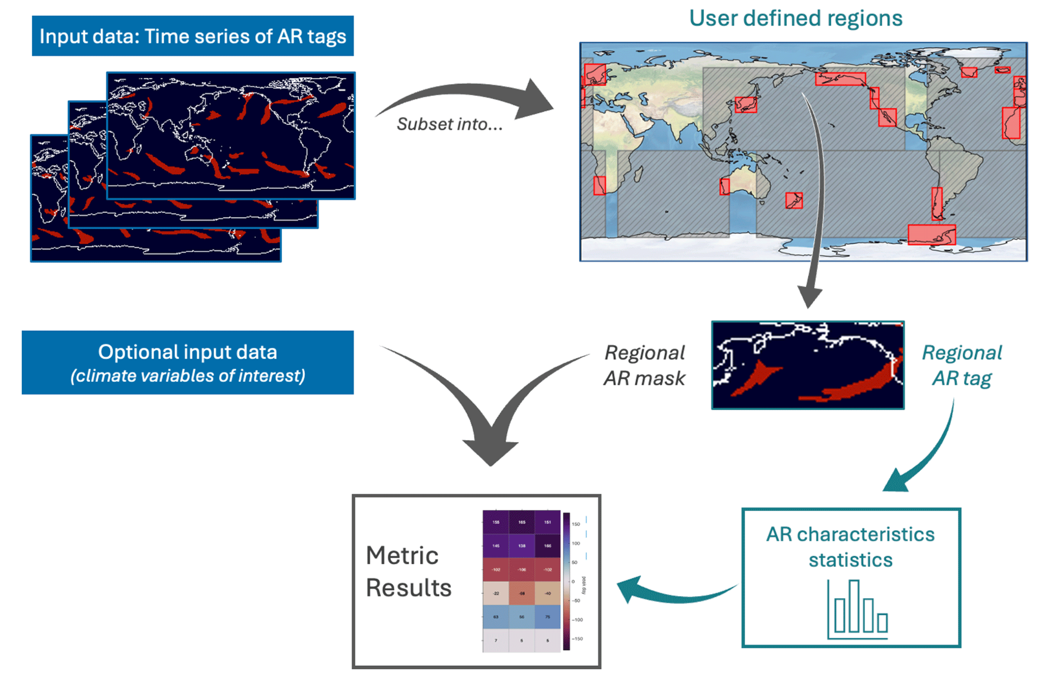
Figure 1 AR metric tool workflow. Input data include time slices of AR tags from ARDTs of user choice and optional climate data associated with ARs. The data are then subset into user-defined rectangular domains (blue boxes for ocean basins, red boxes for landfall regions) for regional tags and masks. User-preferred statistical tools are applied to the regional AR tags to obtain AR characteristics. Finally, AR characteristics and AR masked climate data are presented as metric results.

AR metrics are calculated in user-defined geographic domains. The upper right panel in Fig. 1 shows examples of regions that were selected for landfalling AR diagnostics (red boxes in the panel; lat–long boundaries are listed in Table S3 in the Supplement). These regions, mostly located along the west coast of continents, are known to have frequently observed AR landfalls (Guan and Waliser, 2017; Algarra et al., 2020). We purposely use rectangular region boundaries for simplicity and to avoid masking files; numerous tools are already available for sub-selection of data using latitude–longitude boundaries.

Apart from metrics for AR landfall regions, rectangular region subsetting is also useful for analyzing AR geometric features over global oceans. Currently there are five ocean basins pre-defined in the framework – the North Pacific, South Pacific, North Atlantic, South Atlantic, and southern Indian Ocean (blue boxes in Fig. 1, upper right panel; lat–long coordinates in Table S3). The analysis domains are fully customizable with specified latitude and longitude boundaries from local (depending on spatial data resolution) to global scales.

The regional segments of AR tags can then be used stand-alone as regionally cropped AR objects for feature metrics calculation. In this paper we provide five metrics application examples in Sect. 3, such as AR geometry, frequency, and landfall seasonality. Alternatively, the regional tags can be used as masks for AR-associated weather as well as dynamical and thermodynamical processes. An example of evaluating AR precipitation in climate models is given Sect. 3.

For AR geometrical metrics, statistics gauging the consistency of latitude, longitude, width, length, and size are required as intermediate input data to the workflow. In the examples presented in this paper, we use the BlobStats tool (Ullrich et al., 2021) to calculate these statistics, where latitude and longitude are weighted by the moisture field, width, and length are based on principal component analysis (PCA; Inda-Díaz et al., 2021), and size is based on a count of the number of contiguous grid cells in the feature. This tool can be called and run within the AR metrics framework, although it requires an additional installation. Users can also optionally use their preferred statistical tool for AR geometry calculation and then feed the data back to the metrics workflow.

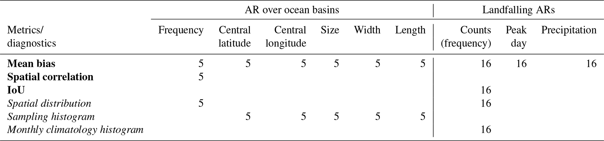
The metrics and diagnostics are integrated into the framework, which can be customized and expanded subject to the objective of research. Table 1 lists all the AR metrics and diagnostics used in this study. The AR metrics are composed of AR properties (as shown in the top row) and evaluation metrics. Similarly, the AR diagnostics are composed of AR properties and statistical diagnostics. The regions that these metrics are applied to are indicated by the numbers in the table.

Table 1 List of AR metrics and diagnostics in this study. Numbers in the table indicate the numbers of regions where the metrics are applied. Each column is one AR property. Bolded items are model evaluation metrics, and items in italic form are diagnostics of AR properties.

2.2 Software structure, coding environment, and data format

The metrics code is open-source and Python-based, and it handles gridded AR tag and climate data using Xarray (https://xarray.pydata.org, last access: 31 December 2023, Hoyer and Hamman, 2017) and its extension xCDAT package (Xarray Climate Data Analysis Tools, https://xcdat.readthedocs.io, last access: 31 December 2023, Vo et al., 2024). It also leverages several utility functions in the PCMDI Metrics Package (PMP; Lee et al., 2024), such as the regional regridding tool, land–sea mask, and portrait plot. These packages are compatible with one another, readily available, and easy to install. The code repository can be accessed at https://github.com/PCMDI/ARMP (last access: 31 December 2023), and relevant wiki documents including a demo Jupyter notebook are provided with installation instructions and application examples.

The code consists of seven major components: workflow controller, I/O, data QAQC, functional utilities, regional statistics, benchmarking metrics, and graphics. It accepts AR masks and climate data files in NetCDF format as input data. Input file names are listed in a pointer file as a configuration parameter to the metrics package. Output files are in NetCDF format for intermediate and diagnostic outputs and JSON format for computed metrics. The regional statistics module integrates a few commonly used statistics for AR properties (e.g., AR frequency and AR precipitation) and newly developed statistics (e.g., AR landfall peak day). External statistical tools, e.g., BlobStats for calculating AR geometry, can also be called from this package. These statistics are then fed into the metrics module. AR metrics included in this framework are described in Sect. 2.3.

The metrics tool can be applied to data with different resolution, domain (e.g., a list of data files with mixed global and regional spatial extent), and coordinate system (e.g., 180 or 360° longitude coordinates; monotonically decreasing latitude coordinates), minimizing the effort required to prepare the input data files. It is compatible with CF-compliant NetCDF files as well as some non-compliant data structures. It also aims to intelligently flag imperfect data, including files with corrupted data values or with an incorrect date/time calendar.

2.3 AR benchmarking metrics

Metrics have been widely used to quantify climate model performance (Taylor, 2001; Gleckler et al., 2008; Wilks, 2011; Zarzycki et al., 2021). In the AR community, a set of common metrics has also been increasingly employed over the past few years, such as mean bias (Guan and Waliser, 2017; Chapman et al., 2019), weighted ensemble mean bias (Massoud et al., 2019), RMSE and relative RMSE (Guan and Waliser 2017), spatial pattern correlation (Chapman et al., 2019; Huang et al., 2020), ratio of spatial standard deviation (O'Brien et al., 2022), and skill scores for assessing AR predictions (Wick et al., 2013; DeFlorio et al., 2018; Nardi et al., 2018) and model performance (Zhang et al., 2024). While these quantitative measures are case-specific and depend on the aim of these studies, there is value in synthesizing commonly used metrics into one comprehensive analysis tool. Here we describe a suite of diverse metrics used in this study, including both commonly used and newly proposed metrics.

2.3.1 Mean bias

We use mean bias to measure how close a climate data product is to an appropriately chosen reference dataset. The statistical significance of the mean bias is measured using the Z test. For the sake of completeness, the mathematical formulas for the mean bias and z score are given in the Appendix. Under this test, the difference between the means of two samples is considered to be statistically significant at the 95 % confidence level if the magnitude of the z score is greater than 1.96. When comparing across different variables, a commonly used measure is the normalized bias, with the data normalized by the standard deviation of the reference field. In this study, we simply use the z score as the normalized bias, as it incorporates both bias and statistical significance in one succinct formula.

2.3.2 Spatial pattern similarity

The spatial pattern correlation is a measure used to quantify the similarity between two spatial fields without reflecting the magnitude of the difference. Here we compute the spatial pattern correlation using the Pearson correlation coefficient. The statistical significance of correlation is determined by the two-tailed p value of the cumulative distribution function (CDF) of the t statistic. The mathematical formula for the Pearson correlation coefficient and its corresponding significance test is given in the Appendix. Given that ARs have notable seasonal and interannual latitudinal shifts, we propose a new method to estimate the effective sample size n_e as the number of principal component analysis (PCA) modes required to explain more than 95 % of the total variance in the AR tag data. The cumulative variance explained by the principal components is expressed as

$$\begin{array}{}\text{(1)}& n_{\mathrm{e}}=min\left\{n_{\mathrm{e}}|{\displaystyle \frac{{\sum }_{i=\mathrm{1}}^{n_{\mathrm{e}}}{\mathit{\lambda }}_i}{{\sum }_{i=\mathrm{1}}^p{\mathit{\lambda }}_i}}>\mathrm{0.95}\right\},\end{array}$$

where λ_i represents the eigenvalues of the spatial correlation matrix of the data, and p is the total number of principal components. Estimating n_e based on ERA5 reanalysis data, we find that the effective sample sizes for spatial pattern correlation are generally small, ranging from 14–27 PCs necessary to explain more than 95 % of total variance for the five ocean basins (Table S4 in the Supplement).

2.3.3 Temporal detection similarity

The AR binary occurrence time series is a time series variable equal to 1 when an AR is present in a given region and zero otherwise. The overlap between two AR occurrence time series is measured by the intersection over union (IoU) metric. The metric is written as

$$\begin{array}{}\text{(2)}& \text{IoU}(A,B)={\displaystyle \frac{\mathrm{\Sigma }|A\cap B|}{\mathrm{\Sigma }|A\cup B|}},\end{array}$$

where A and B are binary AR occurrence time series. The IoU is useful for gauging the degree of temporal similarity of ARs detected in different ARDTs.

3 Metrics applications

In this section, we present five example applications using the metrics tool for assessing ARs in climate models, including evaluation of AR frequency and characteristics, comparison of ARs in high- and low-resolution simulations, sensitivity of ARs to the choice of ARDT, precipitation bias associated with ARs, and landfalling AR seasonality.

3.1 AR tag and climate data

We compare the TE ARDT for the 6-hourly integrated water vapor transport (IVT) data from three reanalysis products – ERA5 (Hersbach et al., 2020), MERRA-2 (Gelaro et al., 2017), and JRA-55C (Kobayashi et al., 2015) to obtain AR tags for reanalyses. Given its longer data record and finer model resolution, we use ERA5 as the default reference in this study. To demonstrate how results are sensitive to the choice of ARDTs, we then use the fixed relative (Mundhenk_v3) tags from ERA5 data.

To evaluate ARs in climate models, we use the archived AR tags from the Atmospheric River Tracking Method Intercomparison Project (ARTMIP) Tier 2 experiment, which is based on the coupled CMIP (Coupled Model Intercomparison Project) model simulations for the historical and 21st century projection periods (Shield et al., 2019a; Rutz et al., 2019; O'Brien et al., 2022). The tag data include six of the CMIP5 models (CCSM4, CSIRO-Mk3-6, CanESM2, IPSL-CM5A-LR, IPSL-CM5B-L, and NorESM1-M) and three of the CMIP6 models (BCC-CSM2-MR, IPSL-CM6A-LR, MRI-ESM2-0). Grid information for these models is listed in Table S1. All the tag data are at 6-hourly temporal frequency. For model evaluation purposes in our application examples, only TE tags from the archive are selected.

We further use simulations from the Energy Exascale Earth System Model (E3SM; Golaz et al., 2019; Caldwell et al., 2019) high-resolution (HR, 0.25°, ∼ 28 km grid) and low-resolution (LR, 1°, ∼ 111 km grid) experiments to examine the sensitivity of ARs to model resolution. Comparison of the grid parameters of the two models is also shown in Table S2. Except for their different horizontal grid spacing, both E3SM-HR and E3SM-LR use an identical set of physical parameters, and the simulations follow a similar protocol of the Coupled Model Intercomparison Project Phase 6 (CMIP6; Eyring et al., 2016).

3.2 Basic AR characteristics in CMIP5 and CMIP6 models

3.2.1 AR frequency

We first analyze the pattern of AR occurrence frequency over a 10-year period (1979–1988) for the five major ocean basins from Sect. 2.2. From the spatial distribution of the AR frequency, we calculate the pattern correlation between selected climate models and ERA5. The spatial pattern correlation coefficient is shown in Fig. 2. Notably the correlations are statistically significant for all models and regions. This suggests that climatologically, all climate models simulate AR density and spatial distribution that broadly resemble reanalysis on the planetary scale. This is evidenced in the spatial AR occurrence density maps in Fig. 3a–b and d–e.

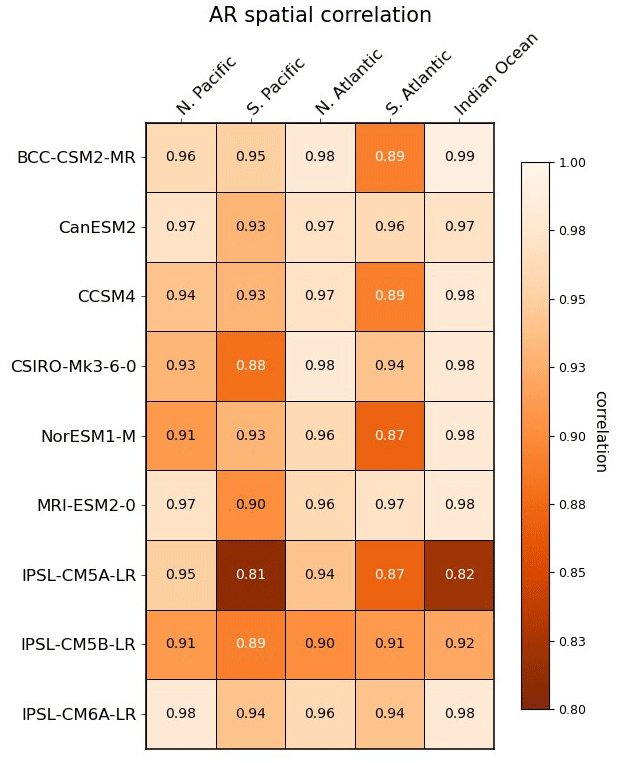
Figure 2 Spatial pattern correlation of AR frequency for the period 1979–1989 between ERA5 and climate models for major ocean basins.

The high spatial correlation (e.g., in Fig. 3, r = 0.88 in the South Pacific and r = 0.98 in the North Atlantic) is mainly a result of the similar spatial gradient (as in Fig. 3a–b and d–e) of the AR frequencies rather than a similar magnitude of frequency at each grid point in the two datasets. For instance, if the AR frequency values on one map are doubled compared to those on the other map, the spatial patterns, or spatial structures of the two, can still be perfectly correlated. Since climatologically ARs are largely clustered along the storm track, with nearly no occurrence over a large portion of the basin domain, it is natural that the pattern correlations are significant in most cases. Similar high pattern correlations of AR frequencies are also noted in other studies (e.g., Huang et al., 2020; Guan et al., 2023). In other words, the spatial correlation coefficient is not that indicative for the magnitude resemblance of the AR spatial frequency. Therefore, these metric results can be better interpreted together with AR frequency maps with spatial gradient.

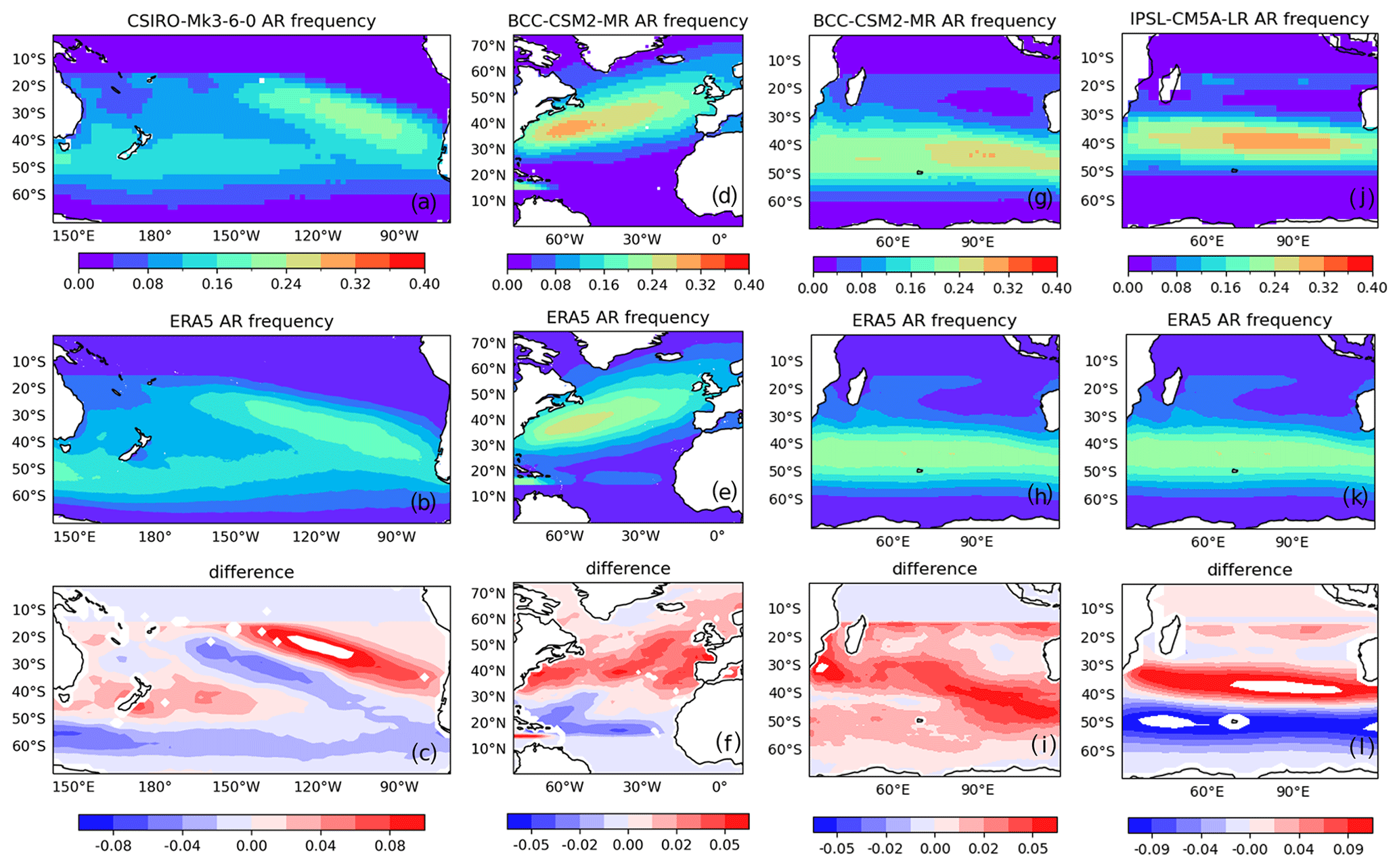
Figure 3 AR frequency in the South Pacific for (a) CSIRO-MK3-6-0, (b) ERA5, and their difference (c) as in panels (a)–(b). Panels (d)–(f), (g)–(i), and (j)–(l) are the same as (a)–(c) but for AR frequency in the North Atlantic for BCC-CM2-MR, Indian Ocean for BCC-CM2-MR, and Indian Ocean for IPSL-CM5A-LR, respectively.

While the spatial correlation coefficient synthesizes the level of pattern consistency, difference maps further reveal spatial discrepancies. For example, Fig. 3c shows that South Pacific AR tracks shift farther towards the Equator in the CSIRO model than in ERA5, while in the North Atlantic basin (Fig. 3f), AR tracks are displaced more poleward in the BCC model. The further north AR location is likely associated with the poleward jet stream bias in CMIP6 models (Bracegirdle et al., 2020; Harvey et al., 2020). Another example is the AR frequency distribution over the Indian Ocean for BCC-CSM-MR (Fig. 3g–i) and IPSL-CM5A-LR (Fig. 3j–l). Even though, compared to ERA5, both models show significant spatial correlation in Fig. 2 (r=0.99 and r=0.82 respectively), the spatial bias pattern in IPSL-CM5A-LR exhibits a more apparent latitudinal shift than in BCC-CSM-MR.

3.2.2 AR geometric features in major ocean basins

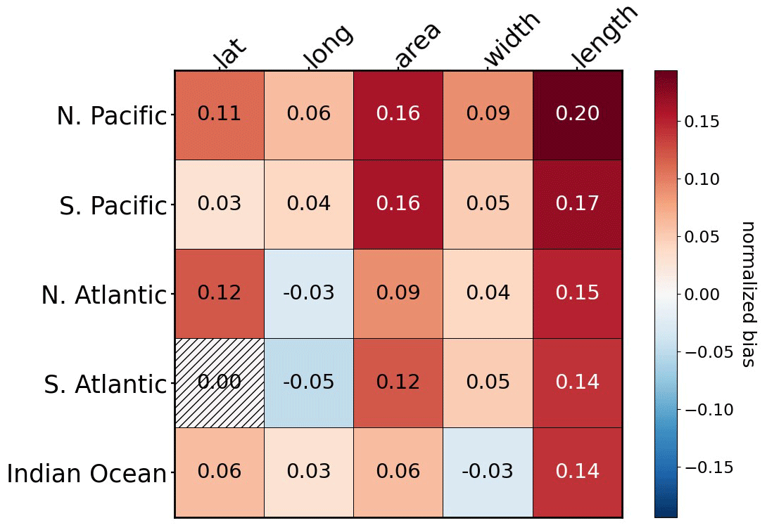
The portrait plots in Fig. 4 show normalized biases (as a z score) of AR characteristics in climate models for the five major ocean basins. Several striking results emerge. For instance, in the North Pacific, the CMIP5 and CMIP6 AR geometries, in terms of width and length, are significantly smaller than the ERA5 reanalysis. One possible cause of such biases is that the AR blobs detected with TE in the relatively lower-resolution climate models are geometrically less curvy and less pointy at the ends; for example, Fig. S2 shows an example time slice of AR blobs in the ERA5 and BCC model. It is clear that the highlighted AR blob in the BCC model exhibits a “cut-off” feature at both ends and is thus shorter in length than the ERA5 reanalysis. And although visually the blob is wider, the PCA-based width is actually narrower due to its less curvy blob geometry. In contrast, for all other ocean basins, the AR sizes (area) are generally bigger in climate models. The figures also show notable latitudinal model AR biases such that, compared to the reanalysis, ARs tend to shift towards higher latitudes in the North and South Atlantic and are biased towards the Equator in the South Pacific and Indian Ocean. To assist in understanding these geographical biases, a set of AR frequency maps over global ocean basins for each climate model is provided in the Supplement.

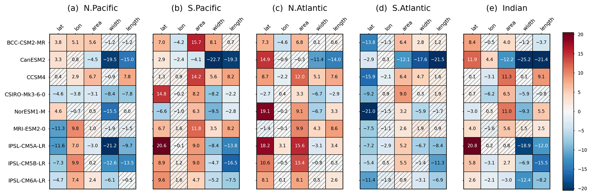
Figure 4 AR characteristic bias (normalized as a Z score) in climate models for major ocean basins. Hatching indicates that the differences are statistically insignificant.

Figure 4 also helps identify outliers of a specific model or variable. For example, although most climate models tend to simulate larger ARs than observed (indicated by the positive values in the area columns), one notable exception is the CanESM2 model, which has significantly smaller AR width, length, and area than other models and ERA5 reanalysis. Taking a closer look at the AR width and length in the North Pacific in Fig. 5, we see that CanESM2 simulates more smaller (< 1.8×10⁶ km²) ARs and fewer larger (> 1.8×10⁶ km²) ARs than the reanalysis, resulting in negative mean biases. This type of histogram helps us better understand the AR distribution discrepancies.

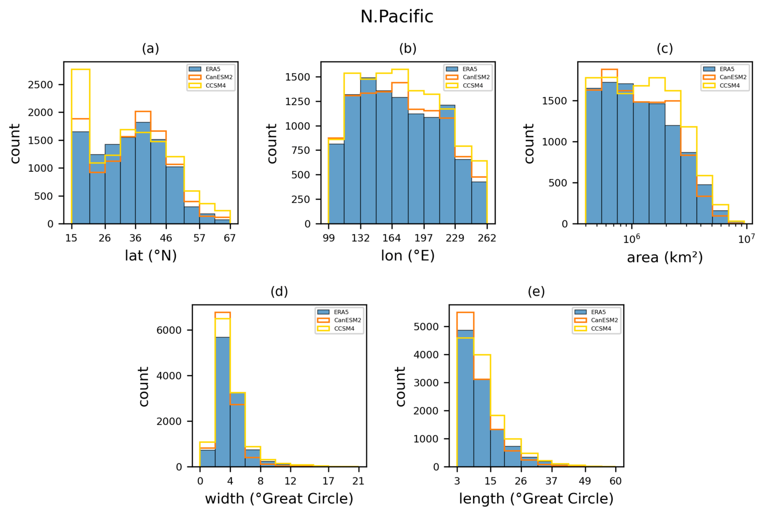
Figure 5 North Pacific AR characteristic distribution for (a) central latitude, (b) central longitude, (c) area, (d) width, and (e) length in the ERA5 reanalysis, CanESM2, and the CCSM4 model.

Another example is from the CCSM4 model simulations. The higher bounds of the model histogram in nearly all fields indicate that the CCSM4 model simulates more ARs than the reanalysis, with bigger size indicated as taller area bars in Fig. 5c. The higher AR counts (∼ 500 more counts than ERA5) in the model are mostly located in the high latitudes and the tropics south of 20° N (Fig. 5a), spreading across all longitudes (Fig. 5b). Figure 5d and e show that the additional ARs in CCSM4 are narrower and/or longer in shape. These differences may arise from various characteristics of the models, such as the dynamical core (e.g., finite volume in CCSM4, T63 triangular spectral truncation in CanESM2, spectral transform in ERA5), grid resolution (see Table S1), and effect of data assimilation (Buizza et al., 2018) in the ERA5 system.

3.3 ARs in high- and low-resolution E3SM simulations

We now apply the metrics and diagnostics identified in Sect. 2.3 to E3SM HR and LR simulations. ARs in both HR and LR exhibit similar structural differences compared to ERA5 (Fig. 6a, b). They are bigger in terms of area, width, and length and biased towards higher latitudes in the North Pacific and South Atlantic, as indicated by the positive numbers. Zonally, ARs in E3SM are more westward distributed in the North Pacific (positive biases) and more eastward distributed in the North Atlantic and South Pacific (negative biases). One difference we see between the two experiments is that in the North Atlantic basin, AR tracks in the HR are shifted more northward than in the LR simulation.

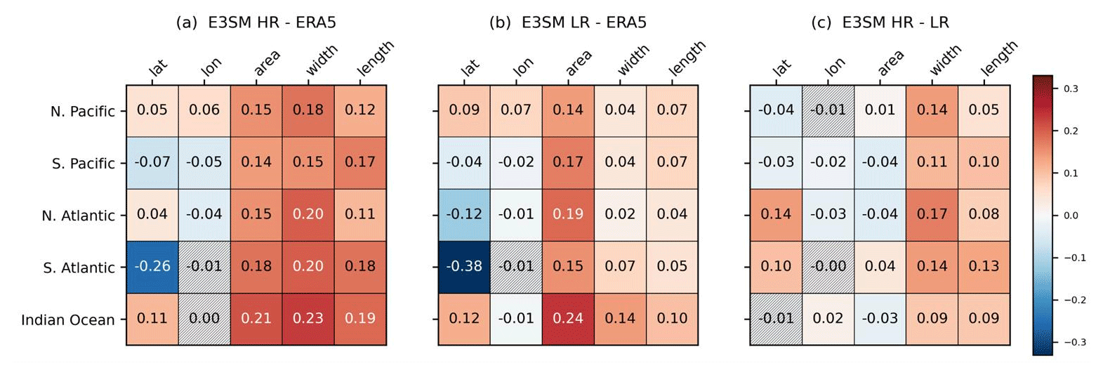
Figure 6 AR characteristic bias in E3SM (a) HR and (b) LR simulations. Panel (c) shows the difference between HR and LR. Hatching indicates that the differences are statistically insignificant.

Figure 6c shows AR differences between the E3SM HR and LR models. The most noticeable difference is that the HR simulates wider and longer ARs than the LR model over all ocean basins. The AR size, in the area column, however, shows mixed results which are not consistent with systematic biases in width and length. This is probably because of different AR geometric properties in the HR and LR simulations. For example, in Fig. S4 in the Supplement, the highlighted AR blob in the North Atlantic is longer but smaller in the LR compared to the one in the HR simulation. Latitudinally, AR distributions a show hemispheric contrast; compared to the LR, ARs in HR are located more southward in the Pacific sector but more northward in the Atlantic sector.

Figure 7 shows the AR characteristic distribution in the North Pacific for E3SM HR, LR, and ERA5. Apparently, E3SM produces more AR events than the reanalysis in nearly all fields and across all scales. We also evaluated the precipitation associated with landfalling ARs in California in both HR and LR simulations, as in Fig. 8. It is notable that both models simulate systematically higher precipitation than ERA5 for all rainfall intensity categories. It is also clear that the precipitation bias in HR simulation is larger than LR simulation, except in the light rainfall (< ∼ 6 mm d⁻¹) category. Similarly, a better topographic representation in the high-resolution version of the model does not improve precipitation simulation, as is also reported in Harrop et al. (2023), especially when the bias in the low-resolution model is substantially high.

Figure 7 AR characteristic distribution of (a) width (° great circle), (b) area (km²), (c) length (° great circle), (d) central latitude (° N), and (e) central longitude (° E) in the North Pacific for ERA5, E3SM HR, and LR simulations.

3.4 Sensitivity of AR characteristics to ARDT

ARDTs are generally threshold-based, mostly using the intensity of moisture transport with some geographical constraints that limit the AR spatial extent and some geometrical constraints that preserve their nature as “long and narrow” filaments of moisture. The different choices made by ARDT developers essentially amount to different definitions of ARs (O'Brien et al., 2022), all of which are qualitatively consistent with the definition in the AMS glossary (Ralph et al., 2018). For example, the Mundhenk algorithm (Mundhenk et al., 2016) calculates integrated water vapor transport (IVT) anomalies relative to the historical period and uses a fixed relative threshold to identify ARs that are above a certain percentile of the historical simulation. The TempestExtremes (TE; Ullrich et al., 2021) method, as another example, uses a relative threshold on the Laplacian of the IVT field rather than the IVT field itself.

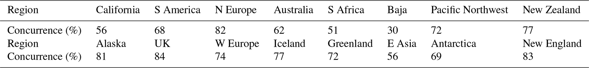
In this application of the metrics package, we examine how ARs in ERA5 are sensitive to the choice of ARDT. In addition to TE-based AR tags, we use AR tags detected using the Mundhenk_v3 algorithm for comparison. Despite significant differences in their associated algorithms, results from ARTMIP showed that their performance was similar and close to the mean among all ARDTs (Shields et al., 2019b). Table 2 shows agreement of landfalling ARs detected using these two ARDTs as percent values of IoU (AR concurrence normalized by total occurrence of the ARs in both methods). The level of consistency ranges from 56 % to 83 %, which suggests that TE and Mundhenk detect ARs concurrently most of the time, but with asynchronous discrepancies, possibly regarding the timing of landfall and the end of the AR life cycle.

Table 2 AR landfall concurrence in Mundhenk and TE, normalized by total counts of AR landfall detected in both ARDTs for different regions. Values are shown in percentage.

For AR characteristics over the oceans, the Mundhenk method detects larger ARs in area, width, and length compared to TE (Fig. 9). Such differences are attributable to the different thresholds for tagging the moisture field in the two ARDTs. The results presented here are obtained from the default criteria; i.e., in TE, ARs are tagged when the Laplacian of the IVT ≦ −20 000, while Mundhenk uses a static 250 kg m⁻¹ s⁻¹ threshold on the IVT field. We might expect different results by altering these threshold numbers. ARs are also present at more northward latitudes with Mundhenk than TE as indicated by positive biases. Zonally, AR distributions exhibit more hemispherical contrast, with Mundhenk showing more westward-located (positive biases) ARs in the Pacific sector but more eastward-located (negative biases) ARs in the Atlantic sector. Apart from TE and Mundhenk, examples of AR geometry patterns from a few other ARDTs are shown in Fig. S3, all showing the results from different criteria for moisture tagging.

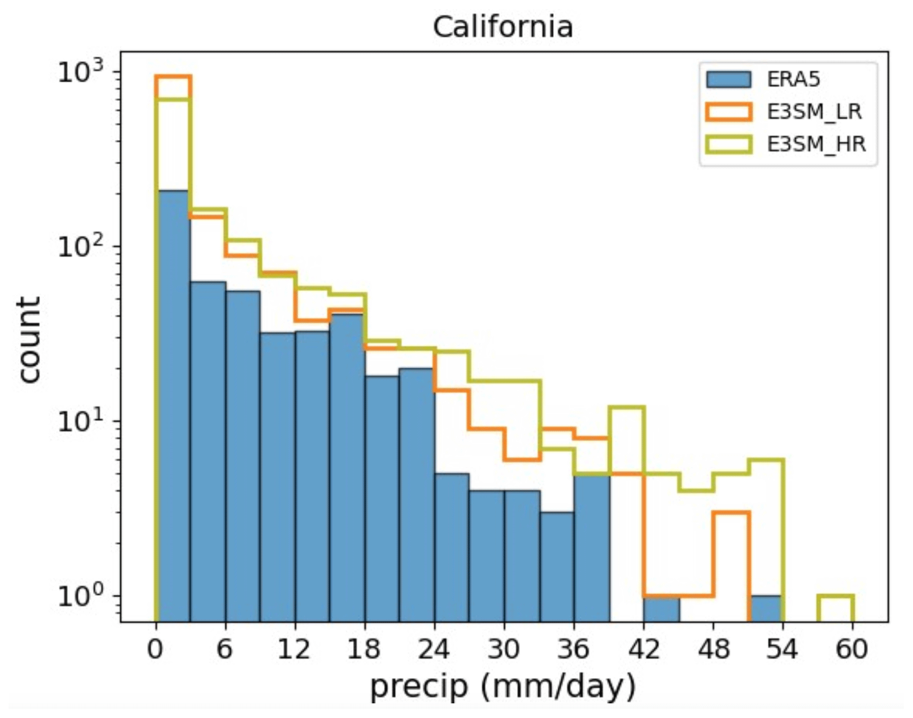
Figure 8 Landfalling AR precipitation histogram in California from 1990–1999 in the ERA5 reanalysis, E3SM HR, and LR simulations.

Figure 9 AR characteristic difference between Mundhenk and TE in ERA5.

3.5 Landfalling AR precipitation in CMIP5/6 models

Apart from comparing AR properties, one useful capability of the ARMP is for analyzing and quantifying any climate fields that are associated with ARs, e.g., precipitation, which is an important indicator of the intensity of a landfalling AR. Here we evaluate landfalling AR precipitation in the CMIP5 and CMIP6 models, with the ERA5 reanalysis and MSWEP (Beck et al., 2017) gridded product as a reference. Figure 10 shows that compared to the observations, landfalling precipitation differences in the models are generally much larger than in reanalysis. The models show dry biases in most regions that are particularly large (up to −7.7 mm d⁻¹) in California, the Pacific Northwest, Iceland, and Greenland.

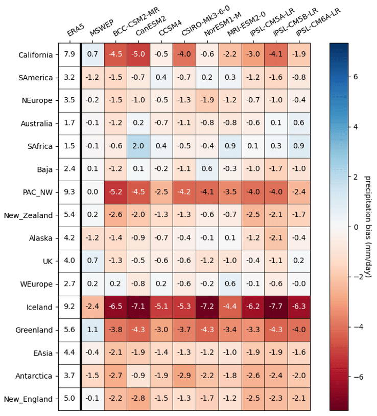
Figure 10 Landfalling AR precipitation bias in climate models relative to ERA5 (the first column). The MSWEP data are also included in the second column as additional reference data, shown as the difference from ERA5.

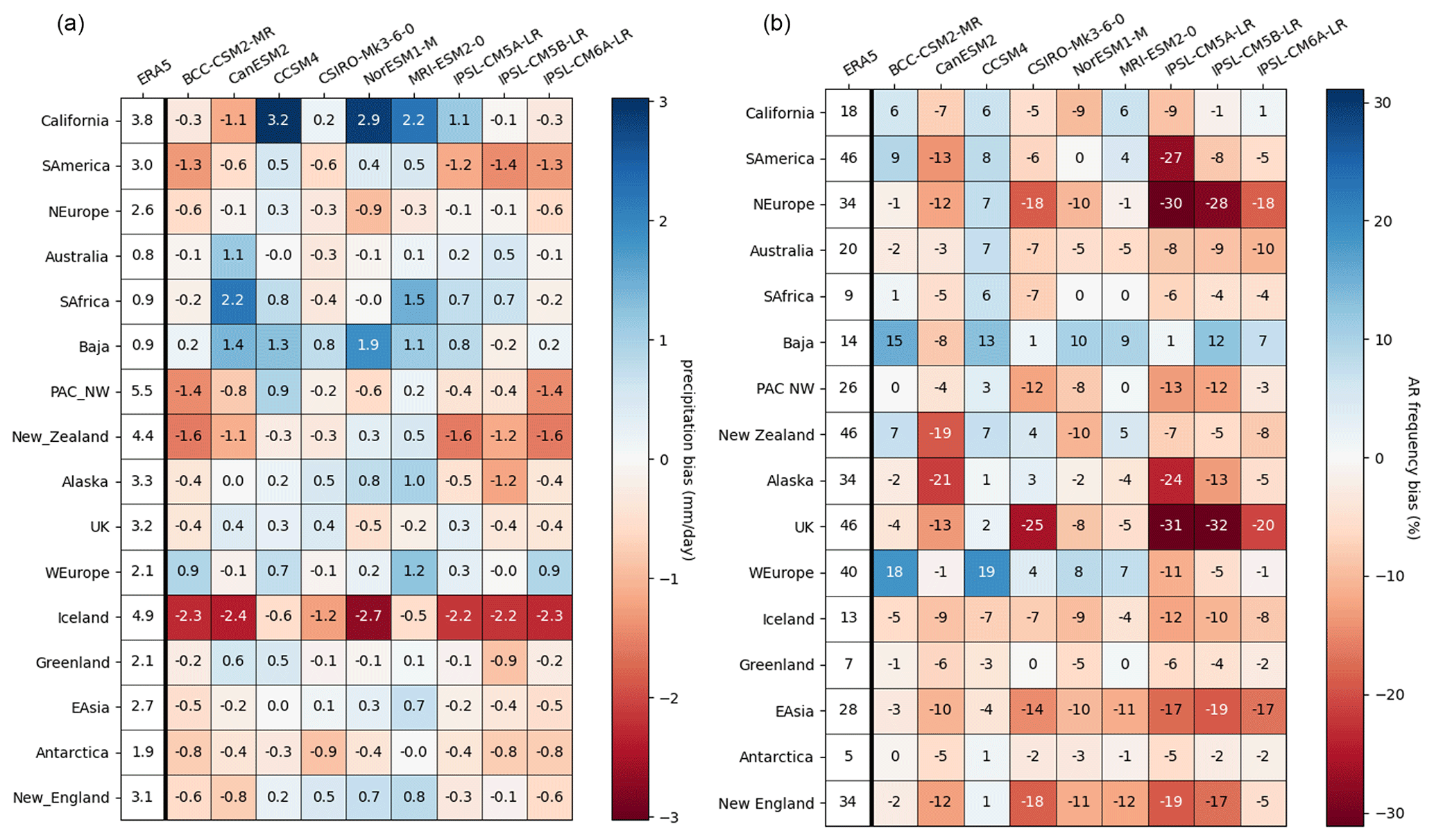
As it is unclear if these biases are mainly due to general precipitation biases or AR activity bias, we further examine model precipitation bias diagnostics regardless of AR activity (Fig. 11a) and AR frequency bias metrics (Fig. 11b) separately. For total precipitation in the models, structural biases as in Fig. 10 are absent, but AR landfall is less frequent in the Pacific Northwest, Iceland, and Greenland. This suggests that the systematic dry AR precipitation biases over these regions are primarily due to the insufficient number of landfalling ARs in the models. For California, similar results do not hold for all the models; for example, total precipitation in CCSM4 is 3.4 mm d⁻¹ higher than the reanalysis, and AR landfall is 6 % more frequent, but the AR-related rainfall has a dry bias of −0.5 mm d⁻¹. This suggests that landfalling ARs in CCSM4 are less intense, suggesting a potential direction for model improvement.

Figure 11 (a) Total precipitation bias and (b) landfalling AR frequency bias.

3.6 Landfalling AR peak day

3.6.1 Comparison among reanalyses

The seasonality of AR landfall is one of the important metrics for understanding AR variability and impacts. Here we analyze landfalling AR seasonality over various regions of the globe among three reanalysis products. We perform a Fourier transform on the 10-year long-term daily mean AR histogram to find its peak date based on the phase of the first Fourier mode. Results indicate that the AR peak days agree well among reanalyses for most regions, with small differences of only a few days. Large discrepancies are noted for Australia and western Africa: in Australia, AR landfall peaks nearly a month behind in JRA-55C compared to MERRA-2, while in western Africa, AR landfall in MERRA-2 peaks 46 d behind ERA5.

Details of these differences are depicted in the histogram plots. For West Africa, AR landfall has two peaks in ERA5 and MERRA-2, one being in September, followed by another peak in November. In ERA5, the peak in November is the main peak, while in MERRA-2, the September peak is comparable to the November peak, resulting in an earlier peak day from the Fourier phase spectrum. JRA-55C, in contrast, has only one peak in November, and the AR landfall event counts are fewer than the other two products over the entire year, indicative of smaller year-to-year variability.

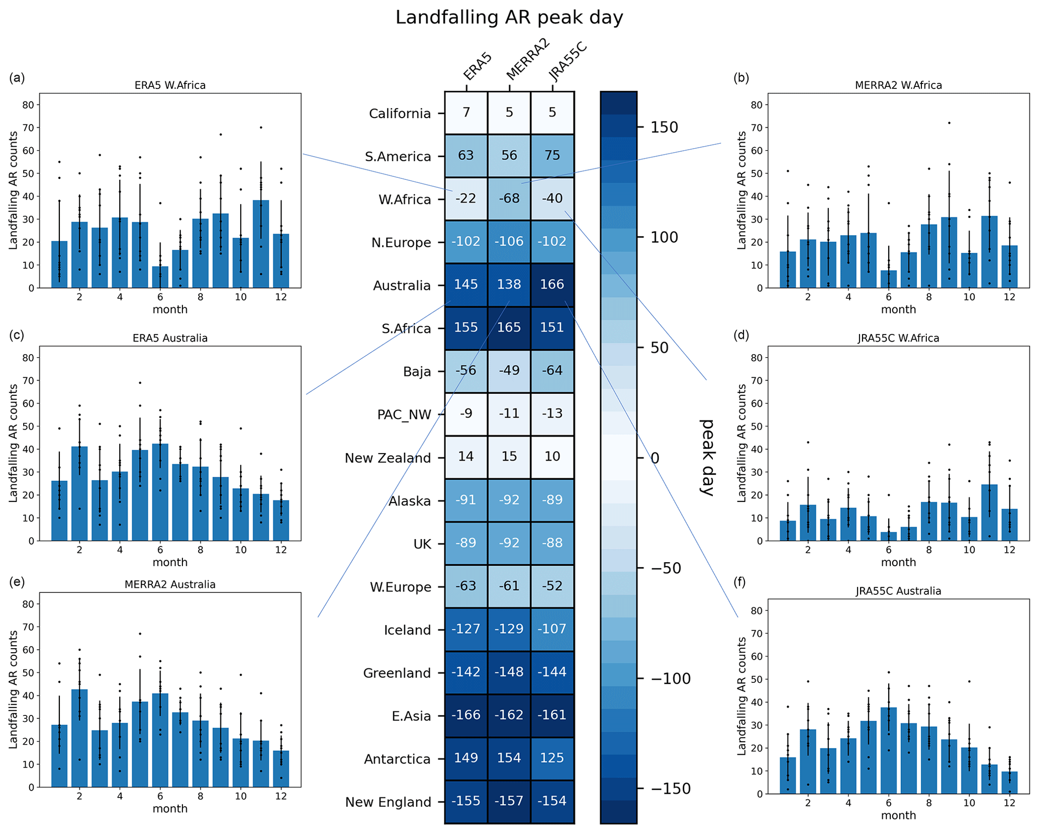
Figure 12 Landfalling AR peak day in ERA5, MERRA-2, and JRA55C reanalysis. Panels (a)–(f) show examples of probability distribution. The height of the blue bars indicates the time mean counts. Black dots represent the peak day for each individual year, and vertical bars are the standard deviation range in the 10-year data from 1979–1988.

The seasonal distribution of AR landfall in Australia in the three reanalyses exhibits similar differences to those in western Africa. In ERA5 and MERRA-2, there are two peaks in February and June, but only one peak is present in JRA-55C in June. This explains the relative late peak day in JRA-55C. While the main peak in ERA5 is in June, in MERRA-2, the main peak is in February, which is consistent with the result from the metrics that MERRA-2 has the earliest peak day. Similarly, JRA-55C has a smaller number of landfalling ARs, although the interannual variability is comparable to the other two reanalyses.

3.6.2 AR seasonality in climate models

Figure 13 shows CMIP5 and CMIP6 model performance in simulating the AR peak season compared to ERA5 reanalysis. To explore how model biases compare to the discrepancies among reanalyses, we also include AR peak day bias for MERRA-2 and JRA-55C reanalysis in the two left columns of the metrics plot. Perhaps unsurprisingly, the model spread is much larger than the spread among reanalysis products, which are tightly constrained by data assimilation.

Figure 13 Landfalling AR peak day bias in reanalyses and models compared with ERA5.

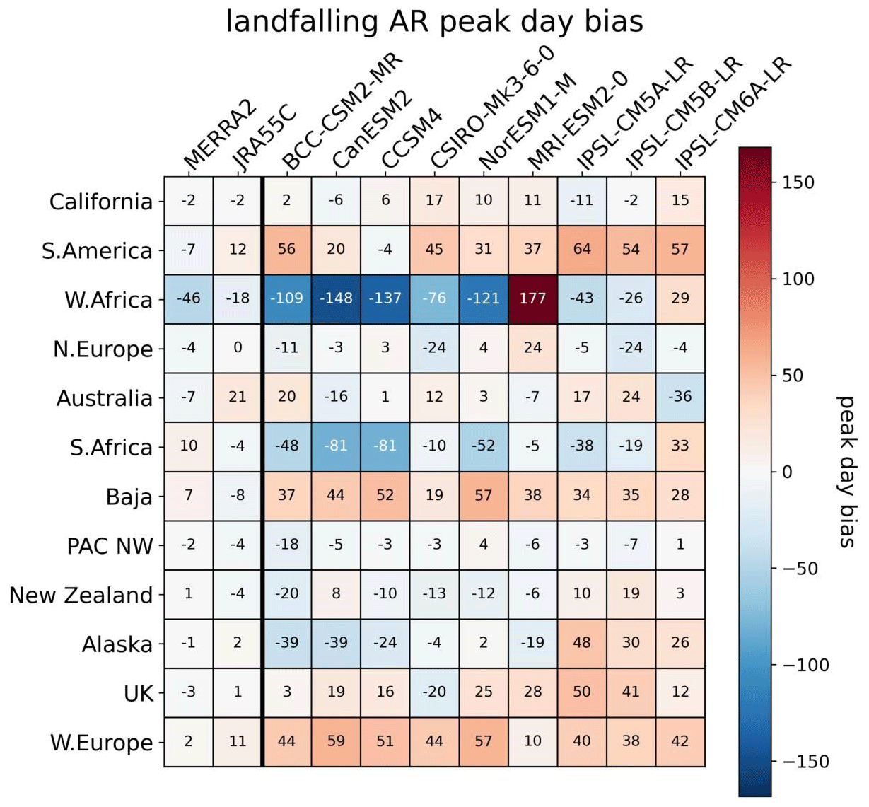
In regions like South America, Baja, the UK, and western Europe, the models show systematic late peak biases, and in South Africa, AR peaks earlier than the reanalyses. The exact cause of these structural biases in the models is likely indicative of persistent and ubiquitous timing issues in the shift of the storm track that is common among models. It is worth noting that the model biases in the West Africa region are significantly larger than other regions, with peak day difference up to 6 months compared to the reanalysis. Looking at the AR count histograms over the course of the year in this region in the CCSM3 and MRI-ESM2-0 models (Fig. 14), it is clear that AR landfall seasonality in both models is completely out of phase with ERA5. This is especially true for the MRI-ESM2-0 model, where AR landfall peaks in June, which is in opposition to the climatology in ERA5. The large discrepancy is probably because of the large spread in the atmospheric circulations in climate models over the West Africa region, as a large spread among CMIP5/6 models in capturing atmospheric dynamic responses (Monerie et al., 2020), the lack of jet–rainfall coupling (Whittleson et al., 2017), and bias in simulating mesoscale convective systems (Jenkins et al., 2002) in climate models are noted. Although high-resolution regional modeling may be capable of improving rainfall in this region (Sylla et al., 2012), the dynamics–rainfall coupling does not appear to be improved in high-resolution global models such as E3SM (Caldwell et al., 2019; Golaz et al., 2019). Therefore, challenges remain in modeling the AR water cycle in western Africa.

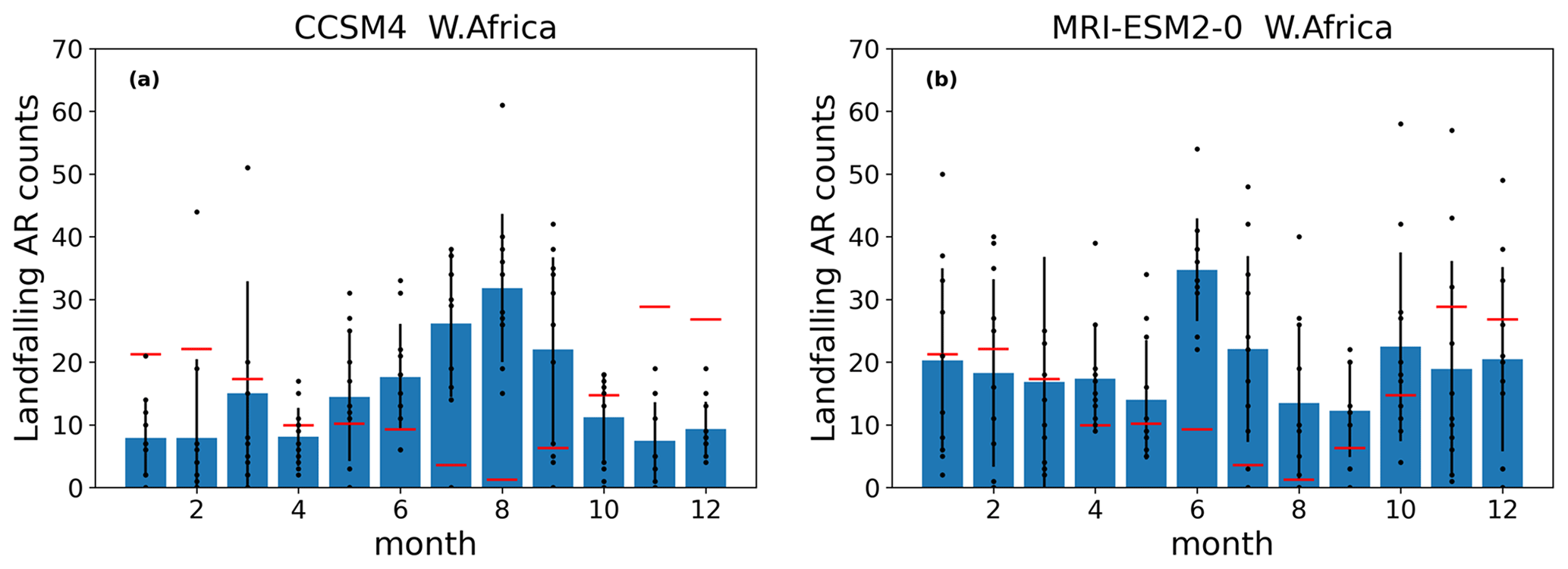
Figure 14 Landfalling AR counts in (a) CCSM4 and (b) MRI-ESM2-0 for the western Africa region. The height of the blue bars indicates the time mean counts. Vertical lines represent the standard deviations. Black dots represent counts for each individual year. Red bars show ERA5 values as the reference.

4 Summary and discussion

In this study we have introduced a metrics framework, namely ARMP, for the objective evaluation of ARs in climate models and reanalysis, and illustrated the potential for its use with five example case studies to illustrate the scope of potential applications. The metrics-based analyses are designed for systematic diagnosis of AR biases in climate models. In our example application applying the package to CMIP5 and CMIP6 models, we have shown that AR tracks in the South Atlantic are positioned farther poleward compared to the ERA5 reanalysis, while in the South Pacific, tracks are biased towards the Equator. Over western Africa, we found that most climate models do a poor job at capturing the AR peak season, while it is generally consistent among reanalyses.

In the application of comparing AR characteristics represented in high- and low-resolution model simulation, while biases are not generally reduced in high-resolution configurations, substantial differences are noted between the two simulations. For example, in the North Atlantic basin, AR tracks in the E3SM-HR are shifted more northward than in the E3SM-LR simulation. In addition to model evaluation and model and reanalysis intercomparison, we have shown how our metrics package can be used to identify structural differences resulting from the choice of AR detector (ARDT). For instance, we demonstrated that ARs detected with the Mundhenk method are systematically larger in size, width, and length compared to TE.

The workflow and metrics presented in this study can be used for a variety of other applications, e.g., to contrast the differences between AR features in historical and future scenarios as simulated by climate models. Objectively quantifying projected changes in landfall frequency, duration, and intervals between landfall events is of particular interest. Further confidence in this and other model evaluation applications can be gained by assessing what impact the choice of the ARDT can have on any conclusions concerning model quality. Our tool makes this and other sensitivity tests more tractable.

Our metrics package assembles a suite of established and newly introduced AR metrics into one framework, facilitating objective evaluation of ARs with a diverse suite of input data, as well as intercomparison of ARs as simulated by multiple climate models. These metrics can be routinely applied for model benchmarking and during development cycles to monitor changes in AR characteristics across model versions or generations and be used to set objective targets for the improvement of models. One expected application is the routine benchmarking of AR in simulations with increasingly higher-resolution models. More frequent metrics evaluation of simulated ARs such as this could further our understanding of model bias and error characteristics and potentially assist developers in making choices associated with new model versions. Furthermore, it can provide a quantitative measure for operational centers to perform near-real-time climate and extreme event impact assessments along with their forecast cycles, which can facilitate the decision-making process.

The collection of metrics included in our metrics package will be augmented to gauge additional AR characteristics. At the time of the submission of this paper, it is being configured to be a part of the PMP. Looking forward, we welcome community contributions to successive development of the package. Inspired by Zarzycki et al. (2021), there is also a potential that these metrics can be applied for research beyond ARs, such as mesoscale meteorological features, regional hydrological extremes such as floods and droughts, and large-scale climate modes.

Appendix A

This section includes mathematical expressions of commonly used model evaluation metrics.

A1 Mean bias

The mean bias is mathematically expressed as

$$\begin{array}{}\text{(A1)}& \overline{b}=\overline{x}-\overline{y},\end{array}$$

where $\overline{x}$ is the arithmetic mean of the test variable x with sample size n, given by

$$\begin{array}{}\text{(A2)}& \overline{x}={\displaystyle \frac{\mathrm{1}}{n}}{\sum }_{i=\mathrm{1}}^n{x}_i.\end{array}$$

Similarly, $\overline{y}$ is the arithmetic mean of the reference variable.

The statistical significance of the mean bias is measured using the Z test, with the test statistics (z score) formulated as

$$\begin{array}{}\text{(A3)}& z={\displaystyle \frac{({\overline{x}}_{\mathrm{1}}-{\overline{x}}_{\mathrm{2}})-({\overline{\mathit{\mu }}}_{\mathrm{1}}-{\overline{\mathit{\mu }}}_{\mathrm{2}})}{\sqrt{\frac{s_{\mathrm{1}}^{\mathrm{2}}}{n_{\mathrm{1}}-\mathrm{1}}+\frac{s_{\mathrm{2}}^{\mathrm{2}}}{n_{\mathrm{2}}-\mathrm{1}}}}},\end{array}$$

where ${\overline{x}}_i$ is the sample arithmetic mean, μ_i is the population mean, s_i is sample variance, and n_i is sample size. A positive z score indicates that the value is above the mean. The higher the z score, the further above the mean the value is, and vice versa. A result is considered statistically significant at the 95 % confidence level if the magnitude of the z score is greater than 1.96.

When comparing across different variables, a commonly used measure is the normalized bias, with the data normalized by the standard deviation of the reference field. In this study, we simply use z score as the normalized bias, as it incorporates both bias and statistical significance in one succinct formula.

A2 Spatial pattern similarity

The spatial pattern correlation is a measure used to quantify the similarity between two spatial fields without reflecting the magnitude of the difference. Here we compute the spatial pattern correlation using the Pearson correlation coefficient:

$$\begin{array}{}\text{(A4)}& r={\displaystyle \frac{{\sum }_{i=\mathrm{1}}^n(x_i-\overline{x})(y_i-\overline{y})}{\sqrt{{\sum }_{i=\mathrm{1}}^n(x_i-\overline{x}{)}^{\mathrm{2}}}\sqrt{{\sum }_{i=\mathrm{1}}^n(y_i-\overline{y}{)}^{\mathrm{2}}}}},\end{array}$$

where x_i and y_i are the values of the two spatial patterns at location i (or grid point i in gridded data product), $\overline{x}$ and $\overline{y}$ are the means of the values of the two patterns, and n is the total number of locations. This equation essentially measures the degree to which the values of the two spatial patterns vary together. If they vary together perfectly, r will be 1. If they vary together inversely, r will be −1. If there's no linear relationship between the patterns, r will be 0.

The statistical significance of correlation is determined by the two-tailed p value of the cumulative distribution function (CDF) of the t statistic as

$$\begin{array}{}\text{(A5)}& p=\mathrm{2}\times (\mathrm{1}-\mathrm{CDF}(t\left)\right).\end{array}$$

The the t statistic t is given by

$$\begin{array}{}\text{(A6)}& t=r\times {\displaystyle \frac{\sqrt{n_{\mathrm{e}}}}{\sqrt{\mathrm{1}-r^{\mathrm{2}}}}},\end{array}$$

where r is the correlation coefficient, and n_e is the effective sample size, although there are a number of methods to estimate the effective geographic sample size (e.g., Griffith, 2013).