Advances in land surface forecasting: a comparison of LSTM, gradient boosting, and feed-forward neural networks as prognostic state emulators in a case study with ecLand

The most useful weather prediction for the public is near the surface. The processes that are most relevant for near-surface weather prediction are also those that are most interactive and exhibit positive feedback or have key roles in energy partitioning. Land surface models (LSMs) consider these processes together with surface heterogeneity and, when coupled with an atmospheric model, provide boundary and initial conditions. They forecast water, carbon, and energy fluxes, which are an integral component of coupled atmospheric models. This numerical parametrization of atmospheric boundaries is computationally expensive, and statistical surrogate models are increasingly used to accelerate experimental research. We evaluated the efficiency of three surrogate models in simulating land surface processes for speeding up experimental research. Specifically, we compared the performance of a long short-term memory (LSTM) encoder–decoder network, extreme gradient boosting, and a feed-forward neural network within a physics-informed multi-objective framework. This framework emulates key prognostic states of the Integrated Forecasting System (IFS) land surface scheme of the European Centre for Medium-Range Weather Forecasts (ECMWF), ecLand, across continental and global scales. Our findings indicate that, while all models on average demonstrate high accuracy over the forecast period, the LSTM network excels in continental long-range predictions when carefully tuned, extreme gradient boosting (XGB) scores consistently high across tasks, and the multilayer perceptron (MLP) provides an excellent implementation time–accuracy trade-off. While their reliability is context-dependent, the runtime reductions achieved by the emulators in comparison to the full numerical models are significant, offering a faster alternative for conducting experiments on land surfaces.

1 Introduction

While the forecasting of climate and weather system processes has long been a task for numerical models, recent developments in deep learning have introduced competitive machine learning (ML) systems for numerical weather prediction (NWP) (Bi et al., 2023; Lam et al., 2023; Lang et al., 2024). Land surface models (LSMs), even though being an integral part of numerical weather prediction, have not yet caught the attention of the ML community. LSMs forecast water, carbon, and energy fluxes, and, in coupling with an atmospheric model, they provide the lower boundary and initial conditions (Boussetta et al., 2021; De Rosnay et al., 2014). The parametrization of land surface states not only affects the predictability of Earth and climate systems on sub-seasonal scales (Muñoz-Sabater et al., 2021) but also affects the short- and medium-range skill of NWP forecasts (De Rosnay et al., 2014). Beyond their online integration with NWPs, offline versions of LSMs provide research tools for experiments on the land surface (Boussetta et al., 2021), the diversity of which, however, is limited by substantial computational resource requirements and often moderate runtime efficiencies (Reichstein et al., 2019).

Emulators constitute statistical surrogates for numerical simulation models that, by approximating the latter, aim for increasing computational efficiency (Machac et al., 2016). While the construction of emulators can itself require substantial computational resources, their subsequent evaluation usually runs orders of magnitude faster than the original numerical model (Fer et al., 2018). For this reason, emulators have found application, for example, in modular parametrization of online weather forecasting systems (Chantry et al., 2021), in replacing the MCMC sampling procedure in Bayesian calibration of ecosystem models (Fer et al., 2018), or in generating forecast ensembles of atmospheric states for uncertainty quantification (Li et al., 2024). Beyond their computational efficiency, surrogate models with high parametric flexibility have the potential to correct process misspecification in a physical model when fine-tuned to observations (Wesselkamp et al., 2024d).

Modelling approaches used for emulation range from low-parametrized, auto-regressive linear models to highly non-linear and flexible neural networks (Baker et al., 2022; Chantry et al., 2021; Meyer et al., 2022; Nath et al., 2022). In the global land surface system M-MESMER, a set of simple AR1 regression models is used to initialize the numerical LSM, resulting in a modularized emulator (Nath et al., 2022). Numerical forecasts of gross primary productivity and hydrological targets were successfully approximated by Gaussian processes (Baker et al., 2022; Machac et al., 2016), the advantage of which is their direct quantification of prediction uncertainty. When it comes to highly diverse or structured data, neural networks have shown to deliver accurate approximations, for example, for gravity wave drags and urban surface temperature (Chantry et al., 2021; Meyer et al., 2022). In most fields of machine learning, specific types of neural networks are now the best approach to representing fit and prediction. One exception is so-called tabular data, i.e. data without spatial or temporal interdependencies (as opposed to vision and sound), where extreme gradient boosting is still the go-to approach (Grinsztajn et al., 2022; Shwartz-Ziv and Armon, 2022).

The ecLand scheme is the land surface scheme that provides boundary and initial conditions for the Integrated Forecasting System (IFS) of the European Centre for Medium-Range Weather Forecasts (ECMWF) (Boussetta et al., 2021). Driven by meteorological forcing and spatial climate fields, it has a strong influence on the NWP (De Rosnay et al., 2014) and also constitutes a standalone framework for offline forecasting of land surface processes (Muñoz-Sabater et al., 2021). The modular construction of ecLand offers potential for element-wise improvement of process representation and thus a stepwise development towards increased computational efficiency. Within the IFS, ecLand also forms the basis of the land surface data assimilation system, updating the land surface state with synoptic data and satellite observations of soil moisture and snow. Emulators of physical systems have been shown to be beneficial in data assimilation routines, allowing a quick estimation and low maintenance of the tangent linear model (Hatfield et al., 2021). Together with the potential to run large ensembles of land surface states at a much reduced cost, this would be a potential application of the surrogate models introduced here.

Long short-term memory (LSTM) networks have gained popularity in hydrological forecasting as rainfall–runoff models for predicting stream flow temperature and also soil moisture (Bassi et al., 2024; Kratzert et al., 2019b; Lees et al., 2022; Zwart et al., 2023). Research on the interpretability of LSTM networks has found correlations between the model cell states and spatially or thematically similar hydrological units (Lees et al., 2022), suggesting the specific usefulness of LSTM for representing variables with dynamic storages and reservoirs (Kratzert et al., 2019a). As emulators, LSTM networks have shown to be useful for sea-surface-level projection in a variational manner with Monte Carlo dropout (Van Katwyk et al., 2023).

While most of these studies trained their models on observations or reanalysis data, our emulator learns the representation from ecLand simulations directly. To our knowledge, a comparison of models without memory mechanisms to an LSTM-based neural network for global land surface emulation has not been conducted before.

We emulate seven prognostic state variables of ecLand, which represent core land surface processes: soil water volume and soil temperature, each at three depth layers, and snow cover fraction at the surface layer. The represented variables would allow their coupling to the IFS, yet the emulators do not replace ecLand in its full capabilities. However, these three state variables represent the core of the current configuration of ecLand. We specifically focus on the utility of memory mechanisms, highlighting the development of a single LSTM-based encoder–decoder model compared to an extreme gradient boosting (XGB) approach and a multilayer perceptron (MLP), which all perform the same tasks. The LSTM architecture builds on an encoder–decoder network design introduced for flood forecasting (Nearing et al., 2024). To compare forecast skill systematically, the three emulators were compared in long-range forecasting against climatology (Pappenberger et al., 2015). In this work, the emulators are evaluated on ecLand simulations only, i.e. on purely synthetic data, while we anticipate their validation and fine-tuning on observations for future work.

2 Methods

2.1 The land surface model: ecLand

The ecLand scheme is a tiled ECMWF scheme for surface exchanges over land that represents surface heterogeneity and incorporates land surface hydrology (Balsamo et al., 2011; ECMWF, 2017). The ecLand scheme computes surface turbulent fluxes of heat, moisture, and momentum and skin temperature over different tiles (vegetation, bare soil, snow, interception, and water) and then calculates an area-weighted average for the grid box to couple with the atmosphere (Boussetta et al., 2021). For the overall accuracy of the atmospheric model, accurate land surface parametrizations are essential (Kimpson et al., 2023), as they, for example, determine the sensible and latent heat fluxes and provide the lower boundary conditions for enthalpy and moisture equations in the atmosphere (Viterbo, 2002). We emulate three prognostic state variables of ecLand that represent core land surface processes: soil water volume (m³ m⁻³) and soil temperature (K) at each of the three depth layers (each at 0–7, 7–21, and 21–72 cm), and snow cover fraction (%) aggregated at the surface layer.

2.2 Data sources

As a training database, global simulation and reanalysis time series from 2010 to 2022 were compiled to zarr format at an aggregated 6-hourly temporal resolution. Simulations and climate fields were generated from ECMWF development cycle CY49R2, ecLand forced by ERA5 meteorological reanalysis data (Hersbach et al., 2020).

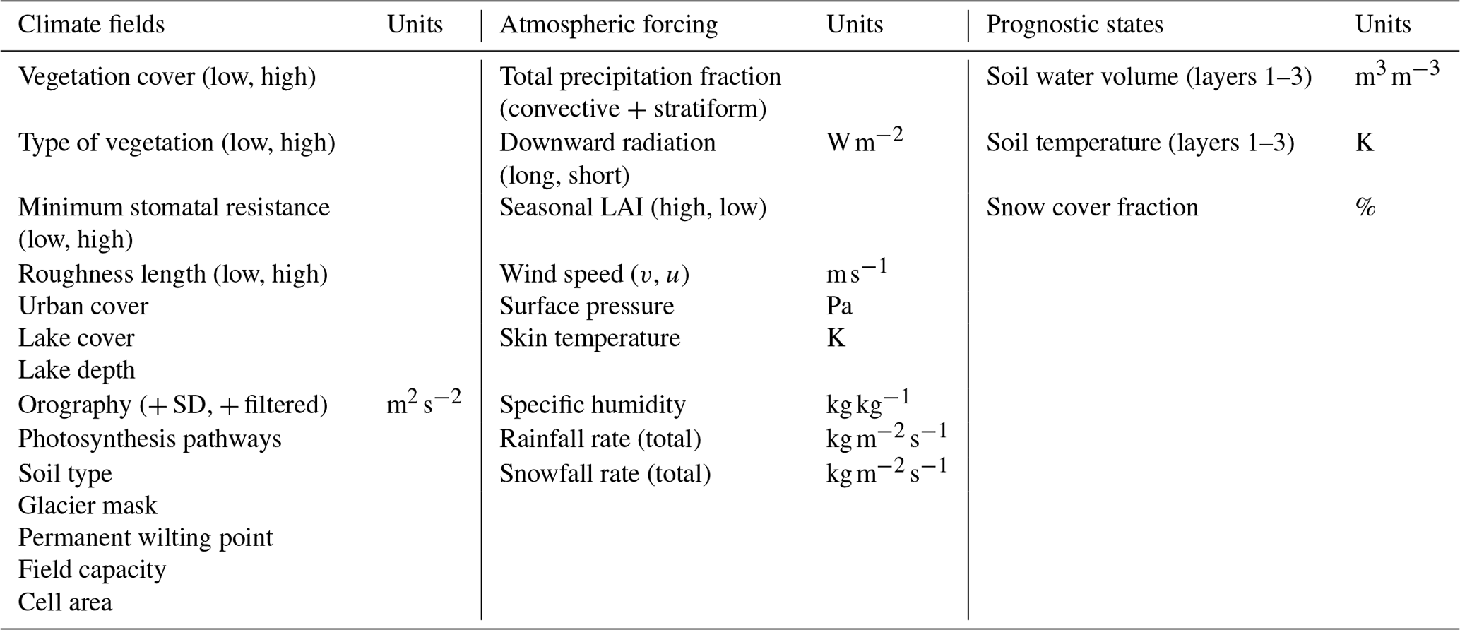
There are three main sources of data used for the creation of the database. The first is a selection of surface physiographic fields from ERA5 (Hersbach et al., 2020) and their updated versions (Boussetta et al., 2021; Choulga et al., 2019; Muñoz-Sabater et al., 2021), used as static model input features (X). The second is a selection of atmospheric and surface model fields from ERA5, used as static and dynamic model input features (Y). The third is ecLand simulations, constituting the model's dynamic prognostic state variables (z) and hence emulator input and target features. A total of 41 static, seasonal, and dynamical features were used to create the emulators; see Table 1 for an overview of input variables and details on the surface physiographic and atmospheric fields below.

2.2.1 Surface physiographic fields

Surface physiographic fields have gridded information of the Earth's surface properties (e.g. land use, vegetation type, and distribution) and represent surface heterogeneity in the ecLand of the IFS (Kimpson et al., 2023). They are used to compute surface turbulent fluxes (of heat, moisture, and momentum) and skin temperature over different surfaces (vegetation, bare soil, snow, interception, and water) and to calculate an area-weighted average for the grid box for coupling with the atmosphere. To trigger all different parametrization schemes, the ECMWF model uses a set of physiographic fields that do not depend on the initial condition of each forecast run or the forecast step. Most fields are constant: surface albedo is specified for 12 months to describe the seasonal cycle. Depending on the origin, initial data come at different resolutions and different projections and are then firstly converted to a regular latitude–longitude grid (EPSG:4326) at ∼1 km at Equator resolution and secondly to a required grid and resolution. Surface physiographic fields used in this work consist of orographic, land, water, vegetation, soil, and albedo fields (see Table 1 for the full list of surface physiographic fields); for more details, see IFS documentation (ECMWF, 2023).

2.2.2 ERA5

Climate reanalyses combine observations and modelling to provide calculated values of a range of climatic variables over time. ERA5 is the fifth-generation reanalysis from ECMWF. It is produced via 4D-Var data assimilation of the IFS cycle 41R2 coupled to a land surface model (ecLand; Boussetta et al., 2021), which includes lake parametrization by Flake (Mironov, 2008) and an ocean wave model (WAM). The resulting data product provides hourly values of climatic variables across the atmosphere, land, and ocean at a resolution of approximately 31 km with 137 vertical sigma levels up to a height of 80 km. Additionally, ERA5 provides associated uncertainties of the variables at a reduced 63 km resolution via a 10-member ensemble of data assimilations. In this work, ERA5 hourly surface fields at ∼31 km resolution on the cubic octahedral reduced Gaussian grid (i.e. Tco399) are used. The Gaussian grid's spacing between latitude lines is not regular, but lines are symmetrical along the Equator; the number of points along each latitude line defines longitude lines, which start at longitude 0 and are equally spaced along the latitude line. In a reduced Gaussian grid, the number of points on each latitude line is chosen so that the local east–west grid length remains approximately constant for all latitudes (here, the Gaussian grid is N320, where N is the number of latitude lines between a pole and the Equator).

Table 1 Input and target features to all emulators from the data sources. The left column shows the observation-derived static physiographic fields, the middle column shows ERA5 dynamic physiographic and meteorological fields, and the right column shows ecLand-generated dynamic prognostic state variables.

2.3 Emulators

We compare a long short-term memory (LSTM) neural network, extreme gradient boosting (XGB) regression trees, and a feed-forward neural network (which we refer to as multilayer perceptron, MLP). To motivate this setup and pave the way for discussing effects of (hyper)parameter choices, a short overview of all approaches is given. All analyses were conducted in Python. XGB was developed in dmlc's XGBoost Python package (https://xgboost.readthedocs.io/en/stable/python/index.html, last access: 11 July 2024). The MLP and LSTM were developed in the PyTorch lightning framework for deep learning (https://lightning.ai/docs/pytorch/stable/, last access: 11 July 2024). Neural networks were trained with the Adam algorithm for stochastic optimization (Kingma and Ba, 2017). Model architectures and algorithmic hyperparameters were selected through combined Bayesian hyperparameter optimization with the Optuna framework (Akiba et al., 2019) and additional manual tuning. The Bayesian optimization minimizes the neural network validation accuracy, specified here as mean absolute error (MAE), over a predefined search space for free hyperparameters with the Tree-structured Parzen Estimator (Ozaki et al., 2022). The resulting hyperparameter and architecture choices which were used for the different approaches are listed in the Supplement.

2.3.1 MLP

For the creation of the MLP emulator, we work with a feed-forward neural network architecture of connected hidden layers with ReLU activations and dropout layers, model components which are given in detail in the Supplement or in Goodfellow et al. (2016). The MLP was trained with a learning rate scheduler. L2 regularization was added to the training objective via weight decay. The size and width of hidden layers, as well as hyperparameters, were selected together in the hyperparameter optimization procedure. Instead of forecasting absolute cell-wise prognostic state variables z_t, the MLP predicts the 6-hourly increment, $\frac{\widehat{\mathrm{d}\mathit{z}}}{\mathrm{d}t}$. It is trained on a stepwise roll-out prediction of future state variables at a pre-defined lead time at given forcing conditions; see details in the section on optimization.

2.3.2 LSTM

LSTM networks are recurrent networks that consider long-term dependencies in time series through gated units with input and forget mechanisms (Hochreiter and Schmidhuber, 1997). In explicitly providing time-varying forcing and state variables, LSTM cell states serve as long-term memory, while LSTM hidden states are the cells' output and pass on stepwise short-term representations stepwise. In short notation (Lees et al., 2022), a one-step-ahead forward pass followed by a linear transformation can be formulated as

$$\begin{array}{c}{\displaystyle }{\mathit{h}}_t,{\mathit{c}}_t=f({\mathit{x}}_t,{\mathit{h}}_{t-\mathrm{1}},{\mathit{c}}_{t-\mathrm{1}},\mathit{\theta })\\ {\displaystyle }{\widehat{\mathit{z}}}_t=\mathit{A}{\mathit{h}}_t+\mathit{b},\end{array}$$

where h_t−1 denotes the hidden state, i.e. output estimates from the previous time step; c_t−1 is the cell state from the previous time step; and θ is the time-invariant model weights. We stacked multiple LSTM cells to an encoder–decoder model with transfer layers for hidden and cell state initialization and for transfer to the context vector (see Fig. 1) (Nearing et al., 2024). A look-back l of the previous static and dynamic feature states is passed sequentially to the first LSTM cells in the encoder layer, while the l prognostic state variables z initialize the hidden state h₀ after a linear embedding. The output of the first LSTM layer cells become the input to the deeper LSTM layer cells, and the last hidden state estimates are the final output from the encoder. Followed by a non-linear transformation with hyperbolic tangent activation, the hidden cell states are transformed into a weighted context vector s. Together with the encoder, the cell state (c_t, s) initializes the hidden and cell states of the decoder. The decoder LSTM cells again take as input static and dynamic features sequentially at lead times $t=\mathrm{1},\mathrm{\dots },\mathit{\tau }$ but not the prognostic states variables. These are estimated from the sequential hidden states of the last LSTM layer cells, transformed to target size with a linear forecast head before prediction. LSTM predicts absolute state variables z_t while being optimized on z_t and $\mathrm{d}{\widehat{\mathit{z}}}_t$ simultaneously; see section on optimization.

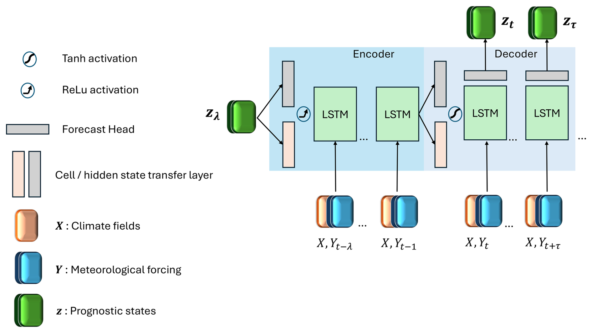
Figure 1 LSTM architecture. The blue shaded area indicates the encoder part, where the model is driven by a look-back λ of meteorological forcing and state variables. The light-blue shaded area indicates the decoder part that is initialized from the encoding to unroll LSTM forecasts from the initial time step t up to a flexibly long lead time of τ.

2.3.3 XGB

Extreme gradient boosting (XGB) is a regression tree ensemble method that uses an approximate algorithm for best-split finding. It computes first- and second-order gradient statistics in the cost function, performing similarly to gradient descent optimization (Chen and Guestrin, 2016), where each new learner is trained on the residuals of the previous ones. Regularization and column sampling aim for preventing overfitting internally. XGB is known to provide a powerful benchmark for time series forecasting and tabular data (Chen and Guestrin, 2016; Chen et al., 2020; Shwartz-Ziv and Armon, 2022). Like the MLP, it is trained to predict the cell-wise increment ${\widehat{\mathrm{d}\mathit{z}}}_t$ of prognostic state variables but only for a one-step-ahead prediction.

2.4 Experimental setup

We distinguish the experimental analysis into three parts that vary in the usage of the training database: (1) model development, (2) model testing, and (3) global model transfer.

The models were developed and for the first time evaluated on a low state resolution (ECMWF's TCO199 reduced Gaussian grid; see section on data sources) and temporal subset from the training database, i.e. on a bounding box of 7715 grid cells over Europe with time series of 6 years from 2016 to 2022. For details on the development database, model selection, and model performances, see Sect. S3 in the Supplement.

The selected models were recreated on a high-state-resolution (TCO399) continental-scale European subset with 10 051 grid cells. Models were trained on 5 years, 2015–2020, with the year 2020 as validation split and evaluated on the year 2021 for the scores we report in the main part. Note that, for the computation of forecast horizons, the two test years 2021 and 2022 were used; see details in the section on forecast horizons. With this same data-splitting setup, the analysis was repeated in transferring the candidates to the low-resolution (TCO199) global data set with a total of 47 892 grid cells. The low global resolution on one hand allowed a systematic comparison of the three models because high-resolution training with XGB was prohibited by the required working memory. On the other hand, this extrapolation scenario created an unseen problem for the models that were selected on a continental and high-resolution scale, which is reflected in the resulting scores.

2.5 Optimization

2.5.1 Loss functions

The basis of the loss function ℒ for the neural network optimization was PyTorch's SmoothL1Loss (https://pytorch.org/docs/stable/generated/torch.nn.SmoothL1Loss.html, last access: 11 July 2024), a robust loss function that combines L1 norm and L2 norm and is less sensitive to outliers than pure L1 norm (Girshick, 2015). Based on a pre-defined threshold parameter β, smooth L1 transitions from L2 norm to L1 norm above the threshold.

SmoothL1Loss ℒ is defined as

$$\begin{array}{}\text{(1)}& \mathcal{L}(\widehat{\mathit{z}},\mathit{z})=\left\{\begin{array}{ll}\mathrm{0.5}(\widehat{\mathit{z}}-\mathit{z}{)}^{\mathrm{2}}\frac{\mathrm{1}}{\mathit{\beta }},& \text{if }|\widehat{\mathit{z}}-\mathit{z}|<\mathit{\beta }\\ |\widehat{\mathit{z}}-\mathit{z}|-\mathrm{0.5}\mathit{\beta },& \text{otherwise},\end{array}\right.\end{array}$$

with β=1. All models were trained to minimize the incremental loss ℒ_s, that is, the differences between the estimates of the seven prognostic state increments ${\widehat{\mathrm{d}\mathit{z}}}_t$ and the full model's prognostic state increments dz_t simultaneously as the sum of losses over all states. We opted for a loss function equally weighted by variables to share inductive biases among the non-independent prognostic states (Sener and Koltun, 2018). When aggregating over all training lead times $t=\mathrm{1},\mathrm{\dots },\mathit{\tau }$, ℒ_s and grid cells $i=\mathrm{1},\mathrm{\dots },p$,

$$\begin{array}{}\text{(2)}& {\mathcal{L}}_{\mathrm{s}}(\widehat{\mathrm{d}\mathit{z}},\mathrm{d}\mathit{z})=\sum _t^{\mathit{\tau }}\sum _i^p{\mathcal{L}}_t({\widehat{\mathrm{d}\mathit{z}}}_{t,i},\mathrm{d}{\mathit{z}}_{t,i}),\end{array}$$

whereas, when computing a roll-out loss ℒ_r stepwise,

$$\begin{array}{}\text{(3)}& {\mathcal{L}}_{\mathrm{r}}(\widehat{\mathrm{d}\mathit{z}},\mathit{z})={\displaystyle \frac{\mathrm{1}}{\mathit{\tau }}}\sum _t^{\mathit{\tau }}\sum _i^p{\mathcal{L}}_t({\mathit{z}}_{t-\mathrm{1},i}+{\widehat{\mathrm{d}\mathit{z}}}_{t,i},{\mathit{z}}_{t,i}).\end{array}$$

Prognostic state increments are essentially the first differences from one time step to the next that are normalized again by the global standard deviation of the model's state increments SD_dz before computation of the loss (Keisler, 2022). Due to the forecast models' structural differences, loss functions were individually adapted:

MLP

The combined loss function for the MLP is the sum of the incremental loss ℒ_s and the roll-out loss ℒ_r. For the roll-out loss ℒ_r, ℒ was aggregated over grid cells p and accumulated after an auto-regressive roll-out over lead times τ before being averaged out by division by τ (Keisler, 2022).

LSTM

The combined loss function for the LSTM is the sum of the incremental loss ℒ_s, where the $\mathrm{d}{\widehat{\mathit{z}}}_t$ were derived from ${\widehat{\mathit{z}}}_t$ after the forward pass and the loss ℒ computed on decoder estimates of prognostic states variables, a functionality that leverages the potential of our LSTM structure.

XGB

Here, we trained only from one time step to the next; i.e. at a lead time of τ=1, the incremental loss ℒ_s=ℒ_r. Without a SmoothL1Loss implementation provided in dmlc's XGBoost, we trained XGB with both the Huber loss and the default L2 loss. The latter initially providing better results, we chose the default L2 norm as the loss function for XGB with the regularization parameter λ=1.

2.5.2 Normalization

As prognostic target variables are all lower-bounded by zero, we tested both z-scoring and max scoring. The latter yielded no significant improvement; thus we show our results with z-scored target variables. For neural network training but not for fitting XGB, static, dynamic, and prognostic state variables were all normalized with z-scoring towards their continental or global spatiotemporal mean $\stackrel{\mathrm{‾}}{z_j}$ and unit standard deviation SD_j as

$$\begin{array}{}\text{(4)}& z_{t,j}={\displaystyle \frac{z_{t,j}-\stackrel{\mathrm{‾}}{z_j}}{{\mathrm{SD}}_j}}.\end{array}$$

Prognostic target state increments were normalized again by the global standard deviation of increments before computing the loss (see Sect. 2.5.1) to smooth magnitudes of increments (Keisler, 2022). State variables were back-transformed to original scale before evaluation.

2.5.3 Spatial and temporal sampling

Sequences were sampled randomly from the training data set, while validation happened sequentially. MLP and XGB were trained on all grid cells simultaneously in both the continental and global setting, while LSTM was trained on the full continental data set but was limited by GPU memory in the global task. We overcame this limitation by randomly subsetting grid cells in the training data into the largest possible, equally sized subsets which were then loaded along with the temporal sequences during the batch sampling.

2.6 Evaluation

Three scores are used for model validation during the model development phase and in validating architecture and hyperparameter selection: the root-mean-square error (RMSE), the mean absolute error (MAE), and the anomaly correlation coefficient (ACC). Firstly, scores were assessed objectively in quantifying forecast accuracy of the emulators against ecLand simulations directly with RMSE and MAE. Doing so, scores were aggregated over lead times τ, grid cells p, or both. The total RMSE was computed as

$$\begin{array}{}\text{(5)}& \text{RMSE}=\sqrt{{\displaystyle \frac{{\sum }_{\mathit{\tau },p}(\mathit{z}-\widehat{\mathit{z}}{)}^{\mathrm{2}}}{n}}},\end{array}$$

with n being the total sample size. Equivalently, the total MAE was computed as

$$\begin{array}{}\text{(6)}& \text{MAE}={\displaystyle \frac{{\sum }_{\mathit{\tau },p}|\mathit{z}-\widehat{\mathit{z}}|}{n}}.\end{array}$$

Beyond accuracy, the forecast skill of emulators was assessed using a benchmark model, measured with the ACC (see below) relative to the long-term naïve climatology c of ecLand, forced by ERA5 (see Sect. 2.2). The climatology is the 6-hourly mean of prognostic state variables over the last 10 years preceding the test year, i.e. the years 2010 to 2020. While climatology is a hard-to-beat benchmark specifically in long-term forecasting, the persistence is a benchmark for short-term forecasting (Pappenberger et al., 2015). For verification against climatology, we compute the target-wise anomaly correlation coefficient (ACC) over lead times as

$$\begin{array}{}\text{(7)}& {\text{ACC}}_{t,j}={\displaystyle \frac{\stackrel{\mathrm{‾}}{({\widehat{z}}_{t,j}-c_{t,j})(z_{t,j}-c_{t,j})}}{\sqrt{\stackrel{\mathrm{‾}}{({\widehat{z}}_{t,j}-c_{t,j}{)}^{\mathrm{2}}}\stackrel{\mathrm{‾}}{(z_{t,j}-c_{t,j}{)}^{\mathrm{2}}}}}}\end{array}$$

at each $t=\mathrm{1},\mathrm{\dots },\mathit{\tau }$, where the overbar denotes averaging over grid cells $i=\mathrm{1},\mathrm{\dots },p$. This way, the nominator represents the average spatial covariance of emulator and numerical forecasts with climatology as the expected sample mean. Hence, it indicates the mean squared skill error towards climatology, and the denominator indicates its variability. The aggregated scores that are shown in Tables 3–5 represent the temporally arithmetic mean. ACC is bounded between 1 and −1, and an ACC of 1 indicates perfect representation of forecast error variability, an ACC of 0.5 indicates a similar forecast error to that of the climatology, an ACC of 0 indicates that forecast error variability dominates and the forecast has no value, and an ACC approaching −1 indicates that the forecast has been very unreliable (Owens and Hewson, 2018). ACC is undefined when the denominator is zero. This is the case when either the emulator anomaly, the ecLand anomaly, or both are zero because forecast and climatology perfectly align or because they cancel out at summation to the mean.

2.6.1 Forecast horizons

Forecast horizons of the emulators are defined by the decomposition of the RMSE (Bengtsson et al., 2008) into the emulator's variability around climatology (i.e. anomaly), ecLand's variability around climatology, and the covariance of both. The horizon is the point in time at which the forecast error reaches saturation level, that is, when the covariance of emulator and ecLand anomalies approaches zero, as does the ACC.

We analysed predictive ability and predictability by computing the ACC for all lead times from 6 h to approx. 1 year, i.e. lead times $t=\mathrm{1},\mathrm{\dots },\mathit{\tau }$, with τ being 1350. As this confounds the seasonality with the lead time, we compute these for every starting point of the prediction, requiring two test years (2021 and 2022).

Forecast horizons based on the emulators' skill in standardized anomaly towards persistence were equivalently computed but with persistence as a benchmark for shorter timescales; this was only done for 3 months, from January to March 2021.

The analysis was conducted on two exemplary regions in northern and southern Europe that represent very different orography conditions and in prognostic land surface states, specifically in snow cover. For details on the regions and on the horizons computed with standardized anomaly skill, see Sects. S1 and S4 respectively.

3 Results

The improvement in evaluation runtimes achieved by emulators toward the physical ecLand was significant. Iterating the forecast over a full test year at 31 km spatial resolution, XGB evaluates in 5.4 min, LSTM evaluates in 3.09 min, and MLP evaluates in 0.05 min (i.e. 3.2 s) on average. In contrast, ecLand integration over a full test year on 16 CPUs at 31 km spatial resolution takes approximately 240 min (i.e. 4 h). The slow runtime of the LSTM compared to the MLP emulator is caused by a spatial chunking procedure that was not optimized for this work but could be improved in the future.

3.1 Aggregated performances

3.1.1 Europe

All emulators approximated the numerical LSM with high average total accuracies (all RMSEs<1.58 and MAEs<0.84) and confident correlations (all ACC>0.72) (see Table 2 and Fig. 2). The LSTM emulator achieved the best results across all total average scores on the European scale. It decreased the total average MAE by ∼25 % towards XGB and by ∼37 % towards the MLP and the total average RMSE by ∼42 % towards XGB and ∼38 % towards the MLP. In the total average ACC, the LSTM scored 20 % higher than the MLP and 15 % than XGB, also being the only emulator that achieved an ACC>0.9. While the MLP outperforms XGB in total average RMSE by ∼5 %, XGB scores better than the MLP in MAE by ∼27 %.

Table 2 Emulator total average scores (unitless), aggregated over variables, time, and space from the European and global model testing. The best model scores for each task are highlighted in bold.

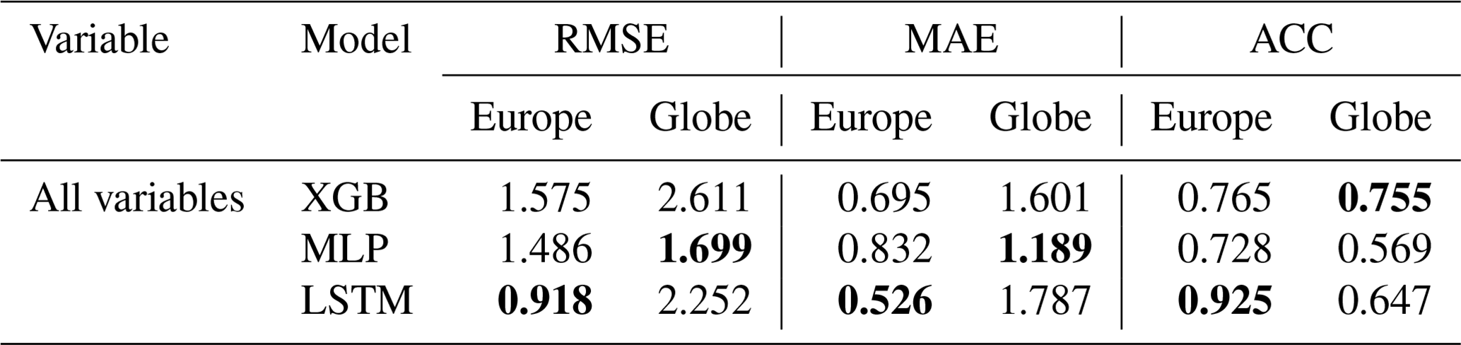
Figure 2 (a) Total aggregated distributions of (log) scores averaged over lead times, i.e. displaying the variation among grid cells. (b) The distribution of the anomaly correlation in space on the European subset (b.1 XGB, b.2 MLP, b.3 LSTM). (c) Model forecasts over test year 2021 for grid cell with minimum and maximum RMSE values (LSTM).

Table 3 Emulator average scores (RMSE, MAE in m³ m⁻³) on soil water volume forecasts for the European subset, aggregated over space and time from the European and global model testing. The best model scores for each task are highlighted in bold.

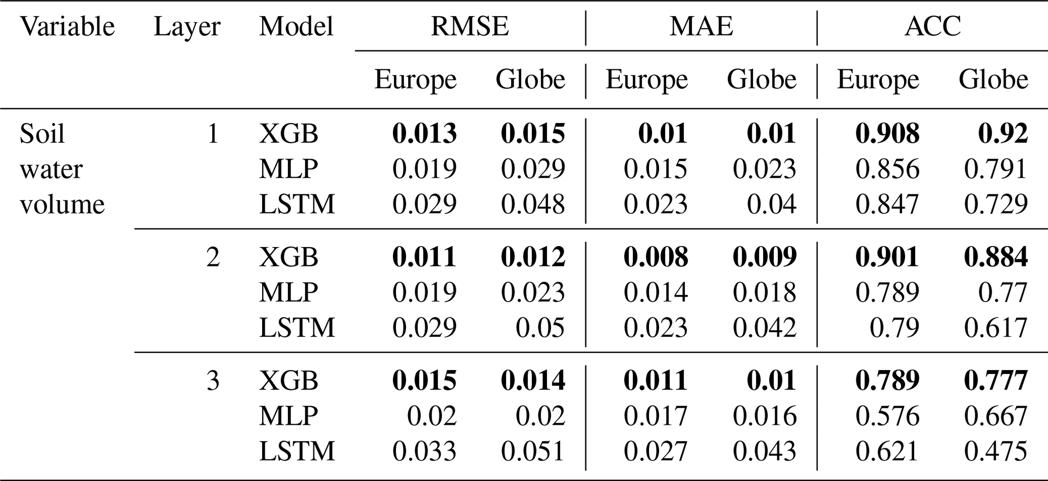
At variable level, results differentiate into model-specific strengths. In soil water volume, XGB outperforms the neural network emulators by up to 60 % (m³ m⁻³) in the first- and second-layer MAEs towards the LSTM and up to over 40 % (m³ m⁻³) towards the MLP (see Table 3). While the representation of anomalies by specifically the LSTM decreases towards lower soil layers with an ACC of only 0.6214 at the third soil layer, it remains consistently higher for XGB with an ACC still >0.789 at soil layer 3.

Table 4 Emulator average scores (RMSE, MAE in K) on soil temperature forecasts for the European subset, aggregated over space and time. The best model scores for each task are highlighted in bold.

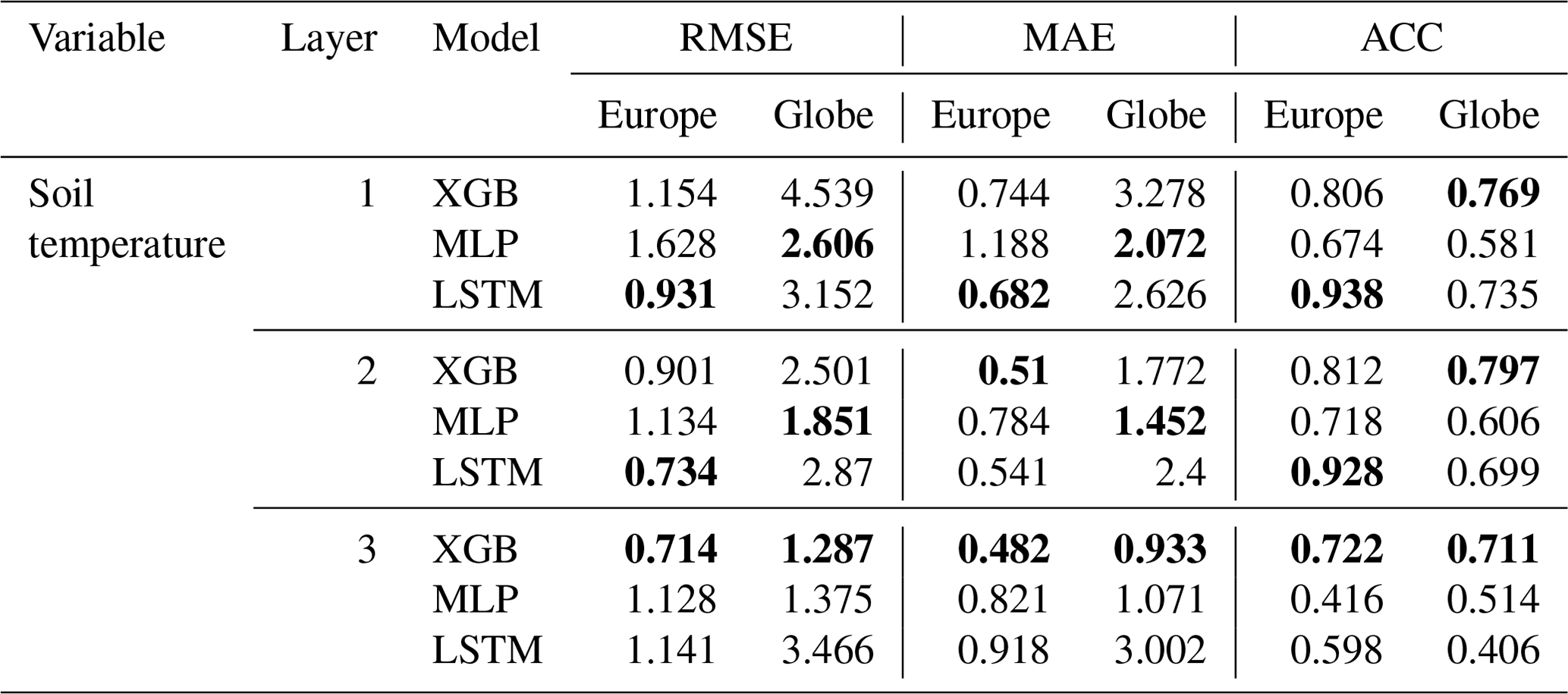
In soil temperature approximation, LSTM achieves best accuracies at higher soil levels with up to 7 % (K) improvement in MAE towards XGB and ACCs >0.92, but XGB outperforms LSTM at the third soil level with a nearly 50 % (K) improvement (see Table 4). The MLP does not stand out with high scores on the continental scale. However, in terms of accuracy, we found an inverse ranking in the model development procedure during which LSTM outscored XGB in soil water volume but struggled with soil temperature approximations; for the interested reader, we refer to the Supplement.

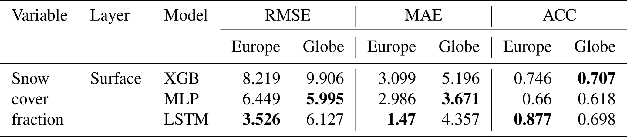
In snow cover approximation, the LSTM emulator enhances accuracies by over ∼50 % in MAE towards both the XGB and the MLP emulator and scores highest in anomaly representation with an ACC of ∼0.87 compared to an ACC of ∼0.66 for the MLP and only ∼0.74 for the XGB (see Table 5).

Table 5 Emulator average scores (RMSE, MAE in %) on snow cover fraction forecasts for the European subset, aggregated over space and time. The best model scores for each task are highlighted in bold.

3.1.2 Globe

Score ranking on the global scale varies strongly from the continental scale (see Table 2). In total average accuracies, the MLP outperforms XGB by over 30 % and LSTM by up to ∼25 % in RMSE and improves MAE more than 15 % towards both. In anomaly correlation, however, it scores last, whereas XGB achieves the highest total average of over 0.75. Consistent with scores on the continental scale is the high performance of XGB in soil temperature (see Table 3). It significantly outperforms the LSTM by ∼60 % (K) in RMSE and up to nearly 75 % (K) in MAE in all layers and outperforms the MLP by up to 50 % (K) in MAE at the top layer. Anomaly persistence for all models degrades visibly towards the lower soil layers, while that of the LSTM does so most relative to MLP and XGB. Like on the continental scale, XGB also outperforms the other candidates in soil temperature forecasts in all but the medium layer, where the MLP gets higher scores in MAE and RMSE but not in ACC (see Table 4). LSTM does not stand out with any scores on the global scale.

3.2 Spatial and temporal performances

3.2.1 Europe

When summarizing temporally aggregated scores as boxplots to a total distribution over space (see Fig. 2a), the long tails of XGB scores become visible, whereas the MLP indicates most robustness. This is reflected in the geographic distribution of scores at the example of ACC (see Fig. 2c.1 and c.2), where the area of low anomaly correlation is largest for XGB, ranging over nearly all of northern Scandinavia, while MLP and LSTM have smaller and more segregated areas of clearly low anomaly correlation. The LSTM shows a homogenously high ACC over most of central Europe except the Alps, while it also degrades in areas of coastal weather conditions, visible along the Norwegian and Spanish coastlines.

3.2.2 Globe

Like the results from the continental analysis, we again find long upper tails of outliers for XGB in total spatial distribution of accuracies, both in RMSE and MAE, and only a few outliers for MLP and LSTM. The anomaly correlation distribution changed towards longer lower tails for MLP and LSTM and a shorter lower tail for XGB. We should, however, take care when interpreting the results of the total average ACC, as it remains largely undefined in regions without much noise in snow cover or soil water volume and globally represents mainly patterns of soil temperature.

3.3 Forecast horizons

Forecast horizons were computed for two European regions, where the northern one represents the area of lowest emulator skill (see Fig. 2b.1–b.3) and the southern one represents an area of stronger emulator skill. Being strongly correlated with soil water volume, these two regions differ specifically in their average snow cover fraction (see Fig. 4, top row). The displayed horizons were computed over all prognostic state variables simultaneously, while their interpretation is related to horizons computed for prognostic state variables separately; for the corresponding figures, refer to the Supplement.

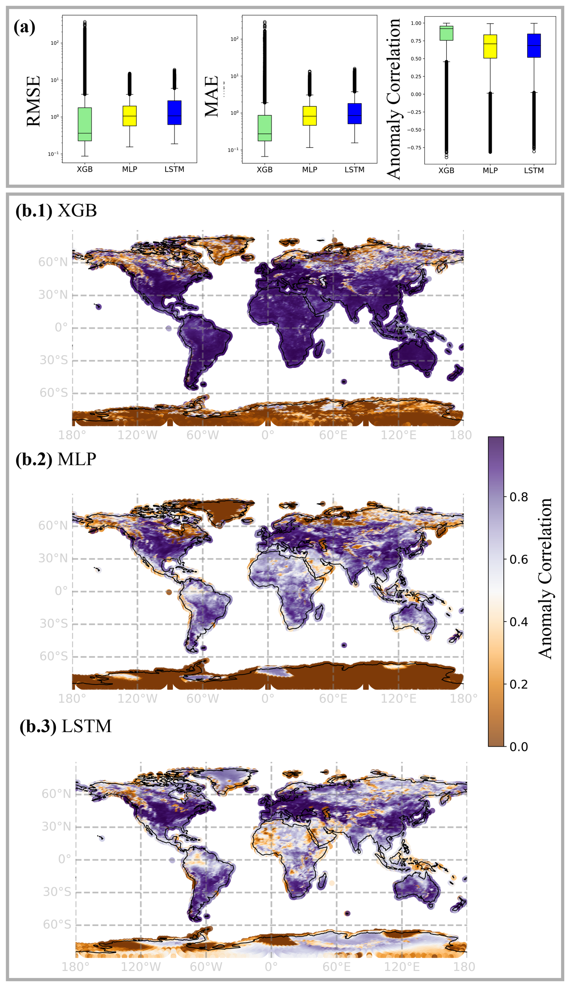
Figure 3 (a) Total aggregated distributions of (log) scores averaged over lead times, i.e. displaying the variation among grid cells. (b) The distribution of the anomaly correlation in space on the global dataset (b.1: XGB, b.2: MLP, b.3: LSTM). Note that ACC remained undefined for regions of low signal in snow cover and soil water volume; see Sect. S4.3.

In the north, predictive skill depended on an interaction of how far ahead a prediction was made (the lead time) and the day of year on which the prediction was made. In the best case, the LSTM, summer predictions were poor (dark patches in Fig. 4 heat maps) but only when initialized in winter. Or, in other words, one can make good predictions starting in winter but not in summer. Vertical structures indicate a systematic model error that appears at specific initialization times and is independent of prediction date, for example, in XGB forecasts that are initialized in May (see Fig. 4 heat maps). Diagonal dark structures in the heat maps indicate a temporally consistent error and can be interpreted as physical limits of system predictability, where the different initial forecast time does not affect model scores.

All models show stronger limits in predictability and predictive ability in the northern European region (see Fig. 4, left column). MLP and XGB struggled with representing seasonal variation towards climatology at long lead times, while LSTM is strongly limited by a systematic error in certain regions. Initializing the forecast on 1 January 2021, MLP drops below an ACC of 80 % repeatedly from initialization on and then to an ACC below 10 % at the beginning of May. LSTM performance is more robust at the beginning of the year but later decreases strongly to less than 10 % ACC in mid-May. On the one hand, this represents two different characteristics of model errors: MLP forecasts for snow cover fraction are less than zero for some grid cells, while LSTM forecasts for snow cover fraction falsely remain at very high levels for some grid cells, not predicting the snowmelt in May (see Sect. S4.1 in the Supplement). On the other hand, this represents a characteristic error due to change in seasonality: the snowmelt in this region in May happens abruptly, and all emulators repeatedly over- or underpredict the exact date.

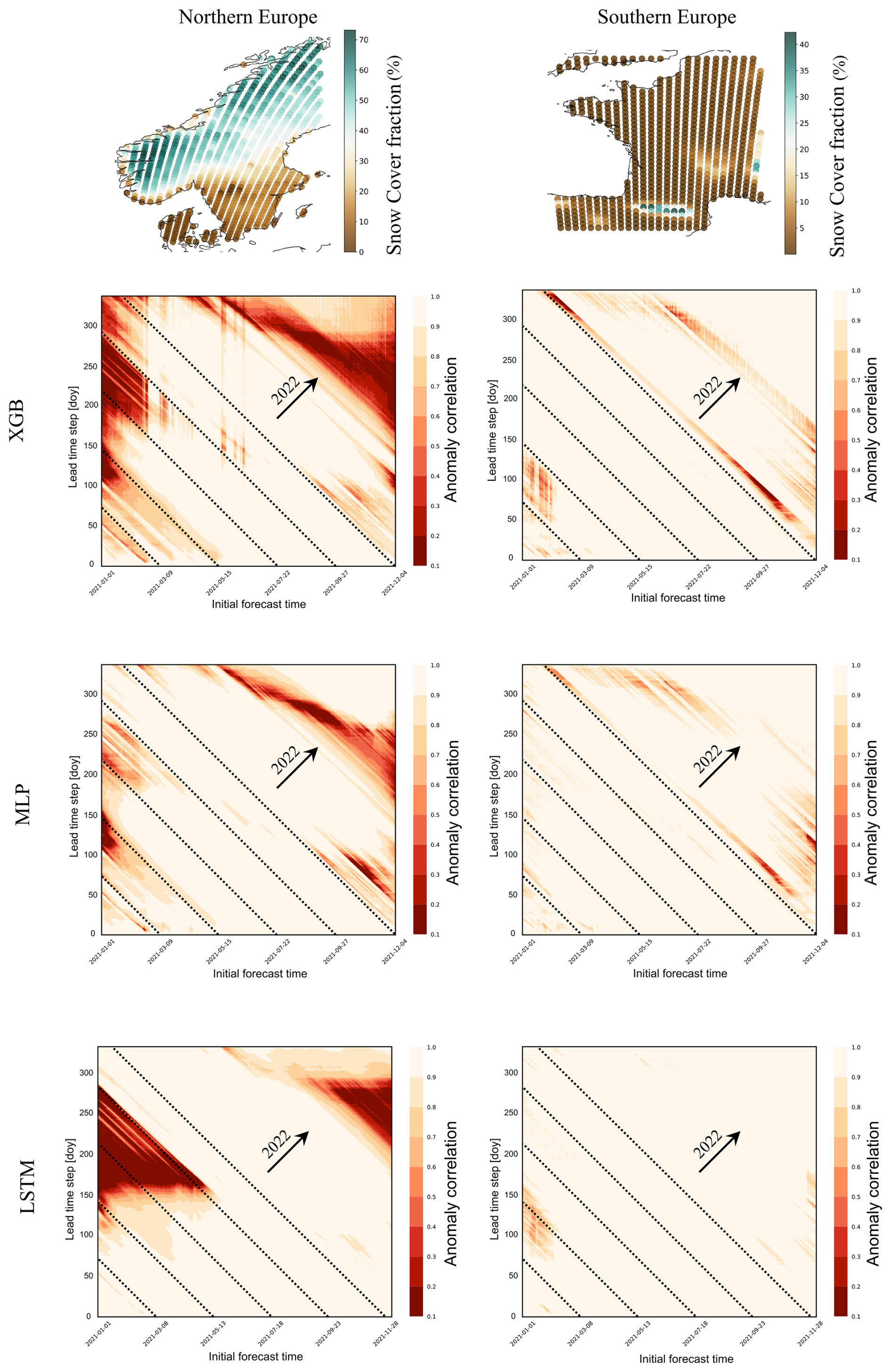
Figure 4 Top row: European subregions for computations of forecast skill horizons and their yearly average snow cover fraction (%), predicted by ecLand. Rows 2–4: emulator forecast skill horizons in the subregions, aggregated over prognostic state variables, computed with the anomaly correlation coefficient (ACC) at 6-hourly lead times (y axis) over approx. 1 year, displayed as a function of the initial forecast time (x axis). The horizon is the time at which the forecast has no value at all, i.e. when ACC is 0 (or below 10 %). The dashed diagonal lines indicate the day of the test year 2021 as labelled on the x axis, and the arrows indicate where forecasts reach the second test year 2022.

4 Discussion

In the comparative analysis of emulation approaches for land surface forecasting, three primary models – long short-term memory (LSTM) networks, multilayer perceptrons (MLPs), and extreme gradient boosting (XGB) – have been evaluated to understand their effectiveness across different operational scenarios. Evaluating emulators over the test period yielded a significant runtime improvement toward the numerical model for all approaches (see Sect. 3). While all models achieved high predictive scores, they differ in their demand of computational resources (Cui et al., 2021), and each one offers unique advantages and faces distinct challenges, impacting their suitability for various forecasting tasks. In this work, we present the first steps towards enabling quick offline experimentation on the land surface with ECMWF's land surface scheme ecLand and towards decreasing computational demands in coupled data assimilation.

4.1 Approximation of prognostic land surface states

The total evaluation scores of our emulators indicate good agreement with ecLand simulations. Among the seven individual prognostic land surface states, emulators achieve notably different scores, and, in the transfer from the high-resolution continental to the low-resolution global scale, their performance rankings change. On average, neural network performances degrade towards the deeper soil layers, while XGB scores remain relatively stable. Also, the neural network scores drop in the extrapolation from continental to global scale, while XGB scores for this task remain constantly high.

In a way, these findings are not surprising. It is known that neural networks are highly sensitive to selection bias (Grinsztajn et al., 2022) and tuning of hyperparameters (Bouthillier et al., 2021), suboptimal choices of which may destabilize variance in predictive skill. Previous and systematic comparisons of XGB and deep neural networks have demonstrated that neural networks can hardly be transferred to new data sets without performance loss (Shwartz-Ziv and Armon, 2022). On tabular data, XGB still outperforms neural networks in most cases (Grinsztajn et al., 2022), unless these models are strongly regularized (Kadra et al., 2021). The disadvantage of neural networks might lie in the rotational invariance of MLP-like architectures, due to which information about the data orientation gets lost, and in their instability regarding uninformative input features (Grinsztajn et al., 2022).

Inversely to expectations and preceding experiments, in the European data set relative to the two other models, the LSTM scored better in the upper-layer soil temperatures than in forecasting soil water volume and decreased in scores towards lower layers with slower processes. For training on observations, the decreasing LSTM predictive accuracy for soil moisture with lead time is discussed (Datta and Faroughi, 2023), but reasons arising from the engineering side remain unclear. In an exemplary case of a single-objective deterministic streamflow forecast, a decrease in recurrent neural network performance has been related to an increasing coefficient of variation (Guo et al., 2021). In our European subregions, the signal-to-noise ratio of the prognostic state variables (computed as the averaged ratio of mean and standard deviation) is up to 10 times higher in soil temperature than in soil water volume states (see Sect. S2.1). While a small signal of the latter may induce instability in scores, it does not explain the decreasing performance towards deeper soil layers with slow processes, where we expected an advantage of the long-term memory.

Stein's paradox tells us that joint optimization may lead to better results if the target is multi-objective but not if we are interested in single targets (James and Stein, 1992; Sener and Koltun, 2018). While, from a process perspective, multi-objective scores are less meaningful than single ones, this is what we opted for due to efficiency. The unweighted linear loss combination might be suboptimal in finding effective parameters across all prognostic state variables (Chen et al., 2017; Sener and Koltun, 2018), yet, being strongly correlated, we deemed their manual weighting inappropriate. An alternative to this provides adaptive loss weighting with gradient normalization (Chen et al., 2017).

4.2 Evaluation in time and space

We used aggregated MAE and RMSE accuracies as a first assessment tool to conduct model comparison, but score aggregation hides model-specific spatiotemporal residual patterns. Furthermore, both scores are variance-dependent, favouring low variability in model forecasts even though this may not be representative of the system dynamic (Thorpe et al., 2013). Assessing the forecast skill over time as the relative proximity to a subjectively chosen benchmark helps to disentangle areas of strengths and weaknesses in forecasting with the emulators (Pappenberger et al., 2015). The naïve 6-hourly climatology as a benchmark highlights periods where emulator long-range forecasts on the test year are externally limited by seasonality, i.e. system predictability, and where they are internally limited by model error, i.e. the model's predictive ability. Applying this strategy in two exemplary European subregions showed that all emulators struggle most in forecasting the period from late summer to autumn, unless they are initialized in summer (see Fig. 3). Because forecast quality is most strongly limited by snow cover (see Sect. S4.1), we interpret this as the unpredictable start of snowfall in autumn. External predictability limitations seem to affect the LSTM overall less than the two other models, and XGB specifically drifts at long lead times.

From a geographical perspective inferred from the continental scale, emulators struggle to forecast prognostic state variables in regions with complicated orography and strong environmental gradients. XGB scores vary seemingly randomly in space, while neural network scores exhibit spatial autocorrelation. A meaningful inference about this, however, can only be conducted in assessing model sensitivities to physiographic and meteorological fields through gradients and partial dependencies. While the goal of this work is to introduce our approach to emulator development, this can be investigated in future analyses.

4.3 Emulation with memory mechanisms

Without much tuning, XGB challenges both LSTM and MLP for nearly all variables (see Tables 2–4). In training on observations for daily short-term and real-time rainfall–runoff prediction, XGB and LightXGB were shown before to perform equally to, or outperform, LSTM networks (Chen et al., 2020; Cui et al., 2021). Nevertheless, models with memory mechanism, such as the encoder–decoder LSTM, remain a promising approach for land surface forecasting regarding their differentiability (Hatfield et al., 2021), their flexible extension of lead times, exploring the effect of long-term dependencies, or inference from the context vector that may help identify the process-relevant climate fields (Lees et al., 2022).

The LSTM architecture assumes that the model is well defined in that the context vector perfectly informs the hidden-decoder states. If that assumption is violated, potential strategies are to create a skip-connection between context vector and forecast head or to consider input of time-lagged variables or self-attention mechanisms (Chen et al., 2020). With attention, the context vector becomes a weighted sum of alignments that relates neighbouring positions of a sequence, a feature that could be leveraged for forecasting quick processes such as snow cover or top-level soil water volume.

Comparing average predictive accuracies across different training lead times indicates that training at longer lead times may enhance short-term accuracy of the LSTM at the cost of training runtime (see Sect. S2). A superficial exploration of encoder length indicates no visible improvement on target accuracies, if not a positive tendency towards shorter sequences. This needs an extended analysis for understanding, yet, without a significant improvement by increased sequence length, GRU cells might provide a simplified and less parametrized alternative to LSTM cells. They were found to perform equally well on streamflow forecast performance before, while reaching higher operational speed (Guo et al., 2021).

4.4 Emulators in application

LSTM networks with a decoder structure are valued for their flexible and fast lead time evaluation, which is crucial in applications where forecast intervals are not consistent. The structure of LSTM is well suited for handling sequential data, allowing it to perform effectively over different temporal scales (Hochreiter and Schmidhuber, 1997). They provide access to gradients, which facilitates inference, optimization, and usage for coupled data assimilation (Hatfield et al., 2021). Nevertheless, the complexity of LSTM networks introduces disadvantages: despite their high evaluation speed and accuracy under certain conditions, they require significant computational resources and long training times. They are also highly sensitive to hyperparameters, making them challenging to tune and slow to train, especially with large data sets.

MLP models stand out for their implementation, training, and evaluation speed with rewarding accuracy, making them a favourable choice for scenarios that require rapid model deployment. They are tractable and easy to handle, with a straightforward setup that is less demanding computationally than more complex models. MLPs also allow access to gradients, aiding in incremental improvements during training and quick inference (Hatfield et al., 2021). Despite these advantages, MLPs face challenges with memory scaling during training at fixed lead times, which can hinder their applicability in large-scale or high-resolution forecasting tasks.

XGB models are highly regarded for their robust performance with minimal tuning, achieving high accuracy not only in sample applications but also in transfer to unseen problems (Grinsztajn et al., 2022; Shwartz-Ziv and Armon, 2022). Their simplicity makes them easy to handle, even for users with limited technical expertise in machine learning. However, the slow evaluation speed of XGB becomes apparent as data set complexity and size increase. Although generally more interpretable than deep machine learning tools, XGB is not differentiable, limiting its application in coupled data assimilation (Hatfield et al., 2021), even though research on differentiable trees is ongoing (Popov et al., 2019).

4.5 Experimentation with emulators

In the IFS, the land surface is coupled to the atmosphere via skin temperature (ECMWF, 2023), the predictability of which is known to be influenced specifically by soil moisture (Dunkl et al., 2021). This is the interface with the numerical model where a robust surrogate could act online to improve forward (i.e. parametrization; Brenowitz et al., 2020) or backward (i.e. data assimilation; Hatfield et al., 2021) procedures, and it motivates the experiment from the perspective of hybrid forecasting models (Irrgang et al., 2021; Slater et al., 2023). However, because offline training ignores the interaction with the atmospheric model, emulator scores will not directly translate to the coupled performance, and of course additional experiments would be necessary (Brenowitz et al., 2020). As the current standalone models, emulators provide a pre-trained model suite (Gelbrecht et al., 2023) and can be used for experimentation on the land surface. The computation of forecast horizons is an example for such an experiment, seen as a step toward a predictability analysis of land surface processes. Full predictability analyses are commonly conducted with model ensembles (Guo et al., 2011; Shukla, 1981), the simulation of which can be done more quickly with emulators than with the numerical model (see evaluation runtimes, Sect. 3).

We want to stress at this point that, to avoid misleading statements, evaluation of the emulators on observations is required. In the context of surrogate models, two inherent sources of uncertainty are specifically relevant: firstly, the structural uncertainty by statistical approximation of the numerical model and, secondly, the uncertainty arising by parametrization with synthetic (computer-model-generated) data (Brenowitz et al., 2020; Gu et al., 2018). Both sources can cause instabilities in surrogate models that could translate when coupled with the IFS (Beucler et al., 2021), but that also should be quantified when drawing conclusions from the standalone models outside of the synthetic domain. Consequently, a reliable surrogate model for online or offline experimentation requires validation, and enforcing additional constraints may be advantageous for physical consistency (Beucler et al., 2021).

5 Conclusion

To conclude, the choice between LSTM, MLP, and XGB models for land surface forecasting depends largely on the specific requirements of the application, including the need for speed, accuracy, and ease of use. Each model's computational demands, flexibility, and operational overhead must be carefully considered to optimize performance and applicability in diverse forecasting environments. When it comes to accuracy, combined model ensembles of XGB and neural networks have been shown to yield the best results (Shwartz-Ziv and Armon, 2022), but accuracy alone will not determine a single best approach (Bouthillier et al., 2021). Our comparative assessment underscores the importance of selecting the appropriate emulation approach based on a clear understanding of each model's strengths and limitations in relation to the forecasting tasks at hand. By developing the emulators for ECMWF's numerical land surface scheme ecLand, we pave the way towards a physics-informed ML-based land surface model that in the long run can be parametrized with observations. We also provide a pre-trained model suite to improve land surface forecasts and future land reanalyses.