Matter (v1): an open-source MPM solver for granular matter

Simulating the mechanics and flow of granular media requires numerical methods that can handle extreme deformations, along with accurate constitutive models capable of capturing phenomena such as elasticity, shear banding, viscous behavior, compressibility, intergranular attractive forces and rate-dependent friction. In pursuit of this, this article introduces Matter, a Material Point Method (MPM) solver equipped with a range of models to describe dry and cohesive granular media. Rooted in a finite strain elastoplastic framework with a multiplicative decomposition of the deformation gradient, this solver features Drucker-Prager models, overstress models, critical state mechanics models as well as the μ(I)-rheology. This includes the recently proposed “critical state μ(I)-rheology model” for cohesive and compressible flows. Moreover, Matter provides a simple way of dealing with complex terrains and introduces a novel material-induced frictional boundary condition. Implemented in C$++$ with few required dependencies and parallelized on shared memory, it represents a lightweight yet computationally efficient option for laptops and desktops.

1 Introduction

Sand, snow, powders and other granular materials typically undergo large deformations, display changes in topology and even experience phase transitions between solid- and fluid-like behavior. Therefore, simulating the dynamics of these media as continua can be a challenging endeavor. As a hybrid Eulerian-Lagrangian method, the Material Point Method (MPM) has since its original formulation in the 1990s established itself as a popular numerical method capable of simulating materials undergoing very large deformations and topology changes. Although the original formulation of MPM is often attributed to Sulsky et al. (1994), it can also be viewed as an extension of Particle-In-Cell (PIC) methods (Harlow, 1964), in particular the FLuid-Implicit-Particle method (FLIP) (Brackbill et al., 1988), to solid mechanics problems, especially problems involving history-dependent materials. Simply put, MPM updates the state of Lagrangian (material) points which carry material properties such as mass, deformation gradient and velocity, while also using an Eulerian grid which facilitates solving the weak form of the momentum balance equation in a manner similar to the Finite Element Method (FEM). As such, MPM offers the advantage of completely avoiding mesh distortion issues in a conceptually simple approach where boundary conditions can be applied as easily as in FEM. Although its similarity to FEM is undoubtedly an advantage, MPM does not inherit all the well-established convergence and stability properties that have been developed over FEM's long history. Nevertheless, earlier criticism related to cell-crossing instabilities and numerical dissipation in MPM has been resolved by the community (e.g., Steffen et al., 2008a; Jiang et al., 2017; Fei et al., 2021). Due to its hybrid nature, MPM comes with a larger memory footprint compared to both FEM and meshless methods such as the Smoothed-Particle Hydrodynamics (SPH). However, it does not necessarily demonstrate a poorer performance compared to SPH as such a meshless scheme requires keeping track of the neighboring discretization points (Raymond et al., 2018; Vacondio et al., 2021). Methods similar in concept to MPM, incorporating the hybrid idea, include the Particle Finite Element Method (PFEM) (Idelsohn et al., 2004) and the Finite Element Method with Lagrangian Integration Points (FEMLIP) (Moresi et al., 2003). In the former, originally conceived for fluid problems and later applied to solids (Oliver et al., 2007), mesh points move in space like Lagrangian particles and remeshing occurs every time the distortion becomes significant (Cremonesi et al., 2020).

There exist several open-source implementations of MPM. Among the first publicly available projects are Uintah MPM (Davison De St. Germain et al., 2000), Nairn MPM (Nairn, 2015), Anura3D (Anura3D, 2017), MPM3D-F90 (Zhang et al., 2017), as well as MPM-GIMP (Wallstedt, 2011) which is an implementation of the algorithm presented in Bardenhagen and Kober (2004). More recent projects include CB-Geo (Kumar et al., 2019), Karamelo (de Vaucorbeil et al., 2021) as well as the Matlab learning environment AMPLE (Coombs and Augarde, 2020). The efficient implementation fMPMM in Matlab (Wyser et al., 2020) and the implementation by Iaconeta et al. (2019) in Kratos (Dadvand et al., 2010) should also be mentioned here. Recently, the computer graphics community has seen a number of MPM implementations in the general framework of the programming language Taichi (Hu et al., 2019), including MLS-MPM (Hu et al., 2018a) and ASFLIP (Fei et al., 2021). The communities have also recently been enriched with several open-source MPM implementations for GPU architectures. One of the earlier is GMPM (Gao et al., 2018) for single-GPU and Claymore (Wang et al., 2020) for multi-GPU architectures. In the context of granular flow, a sparse-memory-encoding GPU framework was recently described by Chen et al. (2025).

Each of the above-mentioned open-source codes offers its own advantages and is typically designed to address specific types of problems, be it in the graphics community or in the engineering communities. In the context of modeling granular matter, however, the existing codes display a limited availability of constitutive laws and rheologies to capture the breadth of such materials which may display elastic behavior, undergo plastic deformation and/or act as a viscous fluid depending on the conditions. Under small/slow deformations, granular media act as elastoplastic solids and appropriate constitutive models must accurately capture their internal frictional behavior and transition into a critical state (Radjai et al., 2017). Under large/fast deformations, granular media behave as a pressure-dependent viscoplastic fluid, and it is generally accepted that dense granular flows follow the so-called μ(I)-rheology (GDR MiDi, 2004; Jop et al., 2006). While materials like sand generally exhibit limited compressibility, snow can undergo much larger variations in its density, e.g., during an avalanche. Even more complicated, cohesive granular media such as snow present additional complexities due to the presence of intergranular forces that influence both their mechanical and flow properties. The study of the flow of cohesive granular media has seen a significant boost in recent years, e.g., with new models or proposed alterations to existing rheologies (Rognon et al., 2006, 2008; Radjai and Richefeu, 2009; Khamseh et al., 2015; Berger et al., 2015; Badetti et al., 2018; Vo et al., 2020; Abramian et al., 2020; Mandal et al., 2020, 2021; Macaulay and Rognon, 2021; Ku et al., 2023; Blatny et al., 2024).

This article introduces Matter (Blatny and Gaume, 2025), an open-source MPM solver encompassing a wide range of models to capture the complex and diverse behavior of granular media, including cohesive and highly compressible granular media. Most notably, it implements the μ(I)-rheology, as well as the recent critical state μ(I)-rheology, both of which can be used with a user-prescribed cohesion and frictional boundary conditions that can optionally be related to the internal friction of the material. It is intended for users studying fundamental granular mechanics as well as those interested in large-scale practical applications. The remainder of this article is organized as follows. First, the governing equations and their discretized form are outlined, followed by an introduction to the finite strain formulation in which all the different constitutive models are formulated. Second, the algorithm is detailed, and the handling of terrains and boundaries is specified. Third, details of the implementations are discussed and verified before finally a few use cases are demonstrated.

2 Theory, discretization and model selection

In this section, MPM is introduced as a numerical continuum scheme for approximating solutions to the momentum and mass conservation laws subject to constitutive models.

2.1 Governing balance laws

The conservation of mass and linear momentum are given by

$$\begin{array}{}\text{(1)}& {\displaystyle \frac{\mathrm{D}\mathit{\rho }(\mathit{x},t)}{\mathrm{D}t}}+\mathit{\rho }(\mathit{x},t)\mathrm{\nabla }\cdot \mathit{v}(\mathit{x},t)=\mathrm{0}\end{array}$$

and

$$\begin{array}{}\text{(2)}& \mathit{\rho }(\mathit{x},t){\displaystyle \frac{\mathrm{D}\mathit{v}(\mathit{x},t)}{\mathrm{D}t}}=\mathrm{\nabla }\cdot \mathit{\sigma }(\mathit{x},t)+\mathit{\rho }(\mathit{x},t)\mathit{g},\end{array}$$

respectively, where ρ is the mass density, v is the velocity, σ is the symmetric Cauchy stress tensor and $\mathrm{D}/\mathrm{D}t$ denotes the material time derivative. In Eq. (2) it is assumed that the only external body force present is the one resulting from the gravitational acceleration g.

2.2 Discretization

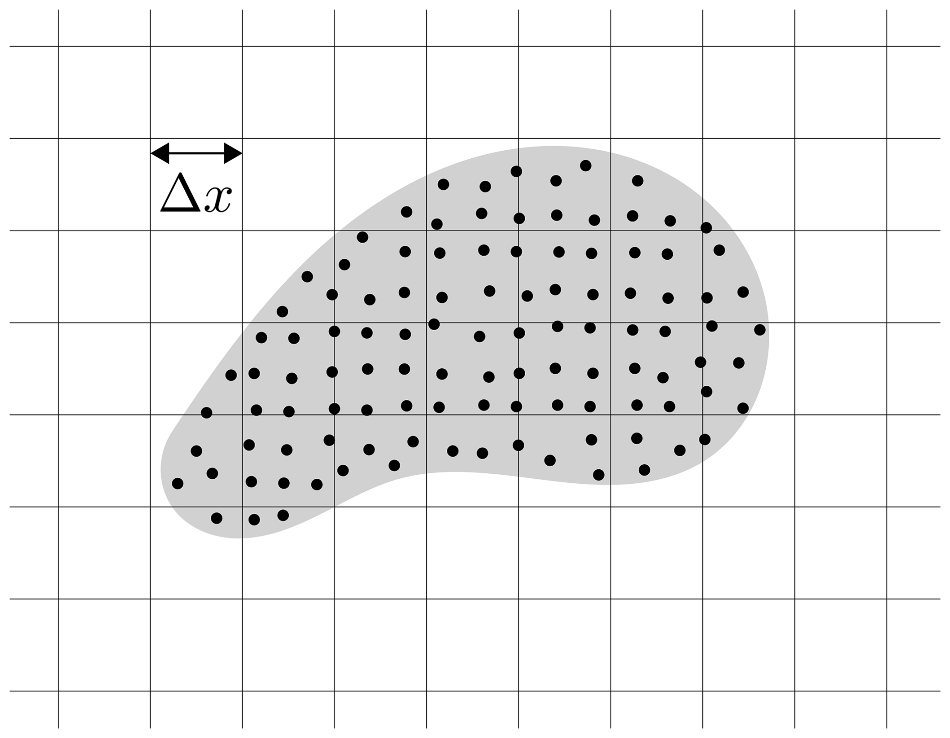
Similarly to FEM, the numerical discretization of MPM starts with the weak form of the governing partial differential equations introduced above. While information is stored on the material points which move in space, the momentum conservation equation is solved on a stationary mesh which usually takes the form of a regular and uniform grid (see Fig. 1).

Figure 1 A body discretized into N_particles particles with N_nodes background grid nodes.

The notation used in this and the next sections can be summarized as follows:

• The domain of the body is described by a finite number N_particles particles and a finite number N_nodes grid nodes.

• Subscript p means the quantity is associated with particle $p\in [\mathrm{1},\mathrm{\dots },N_{\mathrm{particles}}]$.

• Subscript i means the quantity is associated with grid node $i\in [\mathrm{1},\mathrm{\dots },N_{\mathrm{nodes}}]$.

• Superscript n means the quantity is evaluated at time tⁿ associated with time step n∈ℕ.

In order to interpolate between particles and grid nodes, interpolation functions N_i(x) which are strictly non-negative are considered such that ${\mathit{x}}_p={\sum }_i{\mathit{x}}_i{N}_i\left({\mathit{x}}_p\right)\forall p$. Conservation of mass is automatically fulfilled as the total mass of the system ∑_pm_p is the sum of all particle masses which remain constant in time. The volume V_p is, however, not necessarily constant in time.

In the framework of the standard (i.e., updated Lagrangian) MPM the weak form of the momentum conservation equation must be discretized on the grid in the Eulerian configuration. Following closely the derivation in Jiang et al. (2016), Klár (2016) and Pradhana (2017), the spatial and temporal discretization of the momentum equation on the Eulerian grid nodes i assuming a time step size Δt can be derived (neglecting the boundary term) as

$$\begin{array}{}\text{(3)}& {\displaystyle \frac{m_i^n{\mathit{v}}_i^{n+\mathrm{1}}-m_i^n{\mathit{v}}_i^n}{\mathrm{\Delta }t}}=-\sum _p{V}_p^n{\mathit{\sigma }}_p^n\mathrm{\nabla }{N}_{\mathit{i}}\left({\mathit{x}}_p^n\right)+m_i^n\mathit{g}\end{array}$$

where now the left hand side represents the change in momentum while the right hand side represents the internal and external forces. The following remarks should be made:

• This is an updated Lagrangian MPM, which is by far the most popular variant of MPM. This variant can be thought of as the equivalent to the updated Lagrangian FEM discretization, where the quadrature points are now the material points which can move in space and the quadrature weights are now the particle volumes. For this reason, MPM is sometimes referred to as a variant of FEM (de Vaucorbeil et al., 2020b; Nguyen et al., 2023). A total Lagrangian variant of MPM has been proposed by de Vaucorbeil et al. (2020a) in analogy to the total Lagrangian FEM.

• An explicit time discretization is assumed as the variables on the right-hand side of Eq. (3) are evaluated at time tⁿ. While implicit formulations of MPM also exist, explicit MPM remains the most popular in the literature. Although implicit schemes are computationally more expensive than explicit integration (due to the need of solving a nonlinear system of equations at each time step), larger time steps are allowed. This is in contrast to explicit schemes where the time step size must be severely restricted (Sołowski et al., 2021).

• The weak form above is derived with mass lumping. Commonly applied in explicit MPM, mass lumping is a simplification also commonly adopted in explicit FEM schemes. This avoids having to invert the full mass matrix, also bringing about improved stability, however, it may result in increased energy dissipation (Love and Sulsky, 2006; de Vaucorbeil et al., 2020b).

The reader is referred to, e.g., de Vaucorbeil et al. (2020b), Sołowski et al. (2021) and Nguyen et al. (2023) for a more detailed overview of current MPM schemes.

2.3 Finite strain elastoplasticity

In the well-established finite strain framework of a multiplicative decomposition of the deformation gradient F=F^EF^P (Lee, 1969), Matter adopts Hencky's elasticity model which gives a linear relation between the Kirchhoff stress τ=det(F)σ and the Hencky strain ε^E,

$$\begin{array}{}\text{(4)}& \mathit{\tau }={\displaystyle \frac{\partial \widehat{\mathrm{\Psi }}\left({\mathit{\epsilon }}^E\right)}{\partial {\mathit{\epsilon }}^E}}=\mathit{\lambda }\mathrm{tr}\left({\mathit{\epsilon }}^E\right)\mathit{I}+\mathrm{2}G{\mathit{\epsilon }}^E,\end{array}$$

where λ and G are the two Lamé parameters. Here, the strain energy density function $\widehat{\mathrm{\Psi }}$ takes the same functional form as in the Saint-Venant-Kirchhoff model expressed in terms of the Hencky strain instead of the Green strain. The superscript on the Hencky strain serves as a reminder that only the elastic part of the strain promotes stresses. In the context of this isotropic and hyperelastic model, it can be shown that the Kirchhoff stress τ and the Hencky strain ε^E constitute a work-conjugate pair. This, as well as other admirable properties, in particular in relation to hypoelastic models, are presented and derived in Bruhns et al. (1999) and Xiao and Chen (2002).

A yield surface $y(\mathit{\tau },\mathrm{\dots })=\mathrm{0}$, defined through the yield function y, determines the onset of permanent, plastic, deformations. Not considering overstress models (Sect. 2.7), the yield surface defines admissible states y≤0 where plastic deformations are restricted to y=0. The velocity gradient l is assumed additively decomposed as $\mathit{l}={\mathit{l}}^E+{\mathit{l}}^P$. The plastic part of the velocity gradient is determined through the flow rule as

$$\begin{array}{}\text{(5)}& {\mathit{l}}^P=\dot{\mathit{\gamma }}{\displaystyle \frac{\partial g}{\partial \mathit{\tau }}},\end{array}$$

i.e., with a magnitude determined by the plastic multiplier $\dot{\mathit{\gamma }}$ and a direction provided through the plastic potential function g=g(τ). The Kuhn–Tucker conditions must be fulfilled,

$$\begin{array}{}\text{(6)}& \dot{\mathit{\gamma }}\ge \mathrm{0},y\le \mathrm{0},\dot{\mathit{\gamma }}y=\mathrm{0},\end{array}$$

although in the context of overstress models (Sect. 2.7) these restrictions may be relaxed.

Solving the finite strain elastoplastic problem can be accomplished following Simo (1992). An elastic predictor is calculated assuming no plasticity and corrected in case the yield condition is violated. Denoting the Hencky strain ε^E,trial predicted in an elastic step from time tⁿ, this “trial” state is corrected in the return mapping to the new state ${\mathit{\epsilon }}^{E,n+\mathrm{1}}$ at time tⁿ⁺¹ as

$$\begin{array}{}\text{(7)}& {\mathit{\epsilon }}^{E,n+\mathrm{1}}={\mathit{\epsilon }}^{E,\mathrm{trial}}-{\mathit{l}}^P\mathrm{\Delta }t\end{array}$$

which is derived in detail in Blatny (2023). Consequently, the plastic Hencky strain occurring in a time step Δt can be quantified as $\mathrm{\Delta }{\mathit{\epsilon }}^{P,n+\mathrm{1}}={\mathit{l}}^P\mathrm{\Delta }t$.

The above elastoplastic problem can be solved in three or two spatial dimensions. In Matter, the two-dimensional solver option assumes plane strain conditions. From the Lamé parameters, one may construct a Young's modulus $E=\frac{G(\mathrm{3}\mathit{\lambda }+\mathrm{2}G)}{\mathit{\lambda }+G}$ and Poisson's ratio $\mathit{\nu }=\frac{\mathit{\lambda }}{\mathrm{2}(\mathit{\lambda }+G)}$, however, under plane strain conditions, it is often common to define plane strain moduli $E_{\mathrm{2}\mathrm{D}}=\frac{E}{\mathrm{1}-{\mathit{\nu }}^{\mathrm{2}}}$ and ${\mathit{\nu }}_{\mathrm{2}\mathrm{D}}=\frac{\mathit{\nu }}{\mathrm{1}-\mathit{\nu }}$. In the remainder of this article, aligned with the adopted code convention, only (the three-dimensional definitions of) E and ν will be used, and the plane strain definitions can be calculated by the user separately if desired.

Specific elasto-viscoplastic constitutive models that define yield functions and flow rules for granular media are outlined in the remainder of this section, highlighting the wide variety of options available. All models in Matter are formulated in terms of the stress invariants

$$\begin{array}{}\text{(8)}& p=-{\displaystyle \frac{\mathrm{1}}{d}}\mathrm{tr}\left(\mathit{\tau }\right)\end{array}$$

and

$$\begin{array}{}\text{(9)}& q={\displaystyle \frac{\mathrm{1}}{\sqrt{\mathrm{2}}}}\left|\right|\mathrm{dev}\left(\mathit{\tau }\right)\left|\right|\end{array}$$

where p is termed the isotropic pressure and q the equivalent shear stress, using the notation $\left|\right|\mathit{A}\left|\right|=\sqrt{\mathit{A}:\mathit{A}}=\sqrt{\mathrm{tr}\left(\mathit{A}\mathit{A}\right)}$ and $\mathrm{dev}\left(\mathit{A}\right)=\mathit{A}-\frac{\mathrm{1}}{d}\mathrm{tr}\left(\mathit{A}\right)\mathit{I}$ for a symmetric second-order tensor A. The invariant $\sqrt{\mathrm{3}}q$ is often termed the von Mises equivalent stress. Note that the two-dimensional solver, i.e., when d=2, uses $p=({\mathit{\tau }}_{\mathrm{1}}+{\mathit{\tau }}_{\mathrm{2}})/\mathrm{2}$ and $q=\frac{\mathrm{1}}{\mathrm{2}}|{\mathit{\tau }}_{\mathrm{1}}-{\mathit{\tau }}_{\mathrm{2}}|$ where τ₁ and τ₂ denote the principal stresses. This follows from the common choice, under plane strain conditions, of assuming ν=0.5 for yield and plastic flow, see, e.g., Tian (2009), Wojciechowski (2018) and references therein.

2.4 Von Mises

The von Mises model (von Mises, 1913) has a yield function given by

$$\begin{array}{}\text{(10)}& y(p,q)=q-q_y\end{array}$$

where q_y>0 is the von Mises yield stress. The plastic flow rule is generally chosen associative, i.e., g=y. Often used to describe ductile metals, it has also been used to model soils under undrained conditions (Yu, 2006). However, due to its pressure-independency, its applicability for granular media in general is limited.

2.5 Drucker–Prager

The Drucker–Prager model (Drucker and Prager, 1952) extends the von Mises model with pressure-dependency,

$$\begin{array}{}\text{(11)}& y(p,q)=q-q_y\left(p\right),\mathrm{where}{q}_y=\mathit{\mu }p+q_c\end{array}$$

where μ>0 is the internal friction and q_c≥0 is a cohesive stress (or shear strength). Since an associative flow rule would result exclusively in volume increase, i.e., tr(l^P)≠0, this model is often complemented with a non-associative rule, typically using the von Mises plastic potential, i.e., g=q. In Matter, such a flow rule is implemented and combined with the standard “cone tip projection” to address the singularity in the Drucker–Prager yield surface (see e.g., Blatny et al., 2023). As a result of this singularity treatment, some permanent volumetric expansion under tension will occur, which can optionally be suppressed using the volume correction scheme of Pradhana (2017).

A strain-softening Drucker–Prager model is also introduced, in which q_c is no longer a constant, but decreases with the equivalent plastic shear strain ${\mathit{\epsilon }}_S^P$ according to a softening parameter ξ≥0 through

$$\begin{array}{}\text{(12)}& q_c=q_c^{\mathrm{0}}{e}^{-\mathit{\xi }{\mathit{\epsilon }}_S^P}\end{array}$$

where $q_c^{\mathrm{0}}>\mathrm{0}$ is the initial cohesive stress before any deformation occurs. The equivalent plastic shear strain ${\mathit{\epsilon }}_S^P$ is a non-negative scalar defined by

$$\begin{array}{}\text{(13)}& {\mathit{\epsilon }}_S^P=\int \left|\right|\mathrm{dev}\left({\mathit{l}}^P\right)\Vert \mathrm{d}t\approx \sum _n\left|\right|\mathrm{dev}\left(\mathrm{\Delta }{\mathit{\epsilon }}^{P,n}\right)\Vert .\end{array}$$

This formulation of the strain-softening Drucker-Prager model has been used in e.g., Blatny et al. (2021) and Blatny et al. (2023). If ξ→∞, this model promotes a brittle behavior as the cohesion would be immediately removed after initial failure. Other formulations of the strain-softening behavior are also possible.

2.6 Modified Cam–Clay

Critical State Soil Mechanics (CSSM) (Schofield and Wroth, 1968) is a well-established theory in the geomechanics/geotechnics community for describing the mechanics of granular media as elastoplastic solids. This theory is conceived from the idea that there exists a critical state where shear deformations can go on without further changes to volume and stress. In particular, a Critical State Line (CSL) can be defined in (p,q)-space along which all such critical states can exist. Although there are different models that incorporate the main ideas of CSSM, the Modified Cam–Clay (MCC) model is arguably one of the most commonly used in numerical implementations. First formulated by Roscoe and Burland (1968), the MCC model is characterized by an evolving yield surface of ellipsoidal shape in principal stress space.

An MCC yield function that incorporates cohesion can be defined as

$$\begin{array}{}\text{(14)}& y(p,q)=q-q_y\left(p\right),\mathrm{where}{q}_y=\mathit{\mu }\sqrt{\left(p+\mathit{\beta }{p}_c\right)\left(p_c-p\right)},\end{array}$$

where μ>0 defines the slope of the CSL, p_c≥0 is an isotropic compressive strength and β≥0 is a dimensionless measure of cohesion. All critical states (on the CSL) are found on a Drucker-Prager-like surface $q=\mathit{\mu }(p+\mathit{\beta }{p}_c)$, and for exactly this reason the symbol μ is here also used for the slope of the CSL. In Eq. (14), −βp_c represents the isotropic tensile strength, and β can therefore also be described as the ratio between tensile and compressive strength. The case β=0 represents the cohesionless case. In this case, the material can not sustain any tensile stress states. If β>0, there will always be a non-zero tensile strength (unless p_c=0 which represents the stress-free state).

An associative flow rule is used, that is, g=y. As such, both dilation and compaction can occur. An imposed hardening law ensures that the yield surface will shrink or expand, respectively, until critical state is reached. Two hardening laws are considered, both dependent on the equivalent plastic volumetric Hencky strain ${\mathit{\epsilon }}_V^P$ defined as

$$\begin{array}{}\text{(15)}& {\mathit{\epsilon }}_V^P=\int \mathrm{tr}\left({\mathit{l}}^P\right)\mathrm{d}t\approx \sum _n\mathrm{tr}\left(\mathrm{\Delta }{\mathit{\epsilon }}^{P,n}\right).\end{array}$$

The first hardening law is given by

$$\begin{array}{}\text{(16)}& p_c\left({\mathit{\epsilon }}_V^P\right)=p_c^{\mathrm{0}}{e}^{-\mathit{\xi }{\mathit{\epsilon }}_V^P}\end{array}$$

reminiscent of the hardening laws typically used in Cam–Clay models. The second, as presented in Gaume et al. (2018) inspired by Ortiz and Pandolfi (2004), is given by

$$\begin{array}{}\text{(17)}& p_c\left({\mathit{\epsilon }}_V^P\right)=K\sinh \left(-\mathit{\xi }{\mathit{\epsilon }}_V^P+{\sinh }^{-\mathrm{1}}\left({\displaystyle \frac{p_c^{\mathrm{0}}}{K}}\right)\right)\end{array}$$

where in both cases ξ≥0 is a dimensionless parameter and $p_c^{\mathrm{0}}\ge \mathrm{0}$ is an initial compressive strength before any plastic compaction/dilation has occurred. In Eq. (17), $K=\mathit{\lambda }+\mathrm{2}G/d$ is the bulk modulus.

2.7 Overstress models

The above models are restricted to rate-independent plasticity. Viscoplasticity, i.e., rate-dependent plasticity, may be introduced with various approaches. Here, the general overstress model of Perzyna (1963, 1966) is considered. In this approach, a rate-independent yield surface y=0 defines the onset of viscoplastic deformation which occurs for y>0, and a separate expression for the plastic strain rate is imposed. This is in contrast to, e.g., the consistency model (Wang et al., 1997) where the yield surface itself evolves with the rate of deformation and this model can therefore obey all three Kuhn–Tucker relations. Interestingly, both approaches are in the end to a certain extent identical (Heeres et al., 2002).

Following the approach of Perzyna, given a yield stress q_y potentially dependent on p, the plastic shear strain rate ${\dot{\mathit{\gamma }}}_S=\sqrt{\mathrm{2}}\left|\right|\mathrm{dev}\left({\mathit{l}}^P\right)\left|\right|$ is imposed using the formulation of Perić (1993), in particular,

$$\begin{array}{}\text{(18)}& {\dot{\mathit{\gamma }}}_S=\left\{\begin{array}{ll}\mathrm{0}& \mathrm{if}y<\mathrm{0}\\ \frac{\mathrm{1}}{t_{\mathrm{visc}}}\left({\left(\frac{q}{q_y\left(p\right)}\right)}^{\mathrm{1}/s}-\mathrm{1}\right)& \mathrm{if}y\ge \mathrm{0}\end{array}\right.\end{array}$$

where t_visc is a viscous time determining the viscosity of the material and s is a non-negative exponent. The formulation of Perić (1993) has the advantage of recovering the rate-independent limit as s→0 (Neto et al., 2008). The yield stress q_y(p) in Eq. (18) can be chosen as that from von Mises, i.e., Eq. (10), Drucker–Prager, i.e., Eq. (11) or Modified Cam–Clay, i.e., Eq. (14), respectively. Not considering the elastic behavior below yield, the overstress model of Eq. (18) with the choice of a von Mises yield describes Herschel–Bulkley viscoplasticity (Herschel and Bulkley, 1926). If s=1, this reduces to a Bingham fluid (Bingham, 1922).

2.8 The μ(I)-rheology

The μ(I)-rheology (GDR MiDi, 2004; Jop et al., 2006) is a well-established continuum description of dense granular flow where the apparent internal friction depends on a non-dimensional number termed the inertial number I defined by the pressure, shear rate as well as the grain diameter d_g and grain density ρ_g. Following the general idea of Dunatunga and Kamrin (2015), this rheology can be incorporated in an elastoplastic framework as a Drucker-Prager model, Eq. (11), with varying friction μ=μ(I). The typical functional form of μ(I) from Jop et al. (2005) is assumed where μ is bounded by a lower value μ₁ and an upper value μ₂, in particular,

$$\begin{array}{}\text{(19)}& \mathit{\mu }\left(I\right)={\mathit{\mu }}_{\mathrm{1}}+{\displaystyle \frac{{\mathit{\mu }}_{\mathrm{2}}-{\mathit{\mu }}_{\mathrm{1}}}{I_{\mathrm{0}}/I+\mathrm{1}}}={\mathit{\mu }}_{\mathrm{1}}+{\displaystyle \frac{{\mathit{\mu }}_{\mathrm{2}}-{\mathit{\mu }}_{\mathrm{1}}}{\mathit{\omega }\frac{\sqrt{\stackrel{\mathrm{‾}}{p}}}{{\dot{\mathit{\gamma }}}_S}+\mathrm{1}}}\end{array}$$

where I₀ is a constant parameter and for convenience defining $\mathit{\omega }=\frac{I_{\mathrm{0}}}{d_g\sqrt{{\mathit{\rho }}_g}}$. As such, this model has three rheological parameters, μ₁, μ₂ and ω, in addition to the cohesion q_c and the two elastic moduli. In order to treat cohesive problems, i.e., when the pressure p can become negative, the inertial number in Eq. (19) is defined following Berger et al. (2015) and Vo et al. (2020) as

$$\begin{array}{}\text{(20)}& I={\displaystyle \frac{{\dot{\mathit{\gamma }}}_S{d}_g}{\sqrt{\stackrel{\mathrm{‾}}{p}/{\mathit{\rho }}_g}}}\end{array}$$

where an effective pressure

$$\begin{array}{}\text{(21)}& \stackrel{\mathrm{‾}}{p}=p+q_c/{\mathit{\mu }}_{\mathrm{1}}\end{array}$$

is introduced by adding to p the isotropic tensile strength (i.e., the minimal p). Note that, as a result of the particular definitions of p and q in Eqs. (8) and (9), this model is able to retrieve the expected Bagnold solution under (cohesionless) flow on inclined planes when the diagonal stress components can be assumed equal.

Beyond the case of idealized monodisperse granular media, the μ(I)-rheology model in Matter can be considered as simply describing a transition in internal friction from a lower bound μ₁ to an upper bound μ₂. The rate at which this transition occurs is fully governed by the parameter ω. In applications to natural phenomena, such as snow avalanches, where parameter values are less obvious and not as well documented as in systems like, e.g., spherical glass beads, calibration of ω becomes necessary, provided that μ₁ and μ₂ are known or can be reasonably inferred.

2.9 Critical state μ(I)-rheology

The critical state μ(I)-rheology introduced by Blatny et al. (2024) is available in Matter for modeling compressible and cohesive granular flow, and the reader is referred to this article for further details and for the validation of its implementation. This model is conceived as a combination of the MCC model from Sect. 2.6 and the μ(I)-rheology from Sect. 2.8. In essence, this model constructs the CSL to be dependent on the inertial number I such that in the flowing limit it retrieves the properties of the μ(I)-rheology. The inertial number is defined similarly as in Eq. (20), using

$$\begin{array}{}\text{(22)}& \stackrel{\mathrm{‾}}{p}=p+\mathit{\beta }{p}_c\end{array}$$

instead of Eq. (21) following an analogous reasoning, and employing the same functional form of μ(I) as in Eq. (19).

2.10 Summary

As a summary, the various constitutive models in the finite strain elastoplastic framework of Matter are listed below with their key characteristics and typical use cases.

• The von Mises model is suited for ductile materials with negligible pressure effects. It is generally not appropriate for granular media, since it does not include pressure dependence and ignores friction. It is a rate-independent model.

• The Drucker–Prager model applies to granular soils and sands with friction and, if required, cohesion. It introduces a pressure-dependent yield criterion while remaining rate-independent. Optionally, it can be supplied with strain-softening and a scheme for suppressing volume increase.

• The Modified Cam–Clay model is used for both cohesionless and cohesive granular media, particularly clays and soils that exhibit significant plastic volumetric changes. It is capable of capturing hardening/softening, and critical state behavior, and is also rate-independent.

• Overstress models (including Bingham and Herschel–Bulkley) are appropriate for granular suspensions, slurries, or other viscous and creeping flows. They can also be employed for viscous regularization purposes.

• The μ(I)-rheology describes dense granular flows, both cohesive and cohesionless, by incorporating a shear-rate-dependent friction coefficient.

• The critical state μ(I)-rheology extends this framework to dense granular flows with significant plastic volumetric changes, such as snow avalanches. It also relies on a shear-rate-dependent friction coefficient.

In addition to being able to combine the solid and liquid granular phase, the elastoplastic MPM approach has some clear advantages over fluid solvers that implement the μ(I)-rheology. First, due to the introduction of elasticity, there is no need for regularization for low inertial numbers as is otherwise required (Barker and Gray, 2017). Second, no special treatment of the free-surface is necessary as MPM by construction handles this naturally. Third, connectivity to the boundary is not required and lift-offs are trivially handled.

3 Algorithm

In this section, Matter's algorithm is introduced in the context of finite strain elastoplasticity.

The MPM community has distinguished schemes that update the particle stresses before or after the grid velocity updates, the former known as Update Stress First (USF) and the latter as Update Stress Last (USL). The algorithm described here considers USL as well as the Modified USL (MUSL) (Sulsky et al., 1995). Notably, USL schemes are by some claimed to be superior to USF in terms of stability and convergence (Wallstedt and Guilkey, 2008; de Vaucorbeil et al., 2020b).

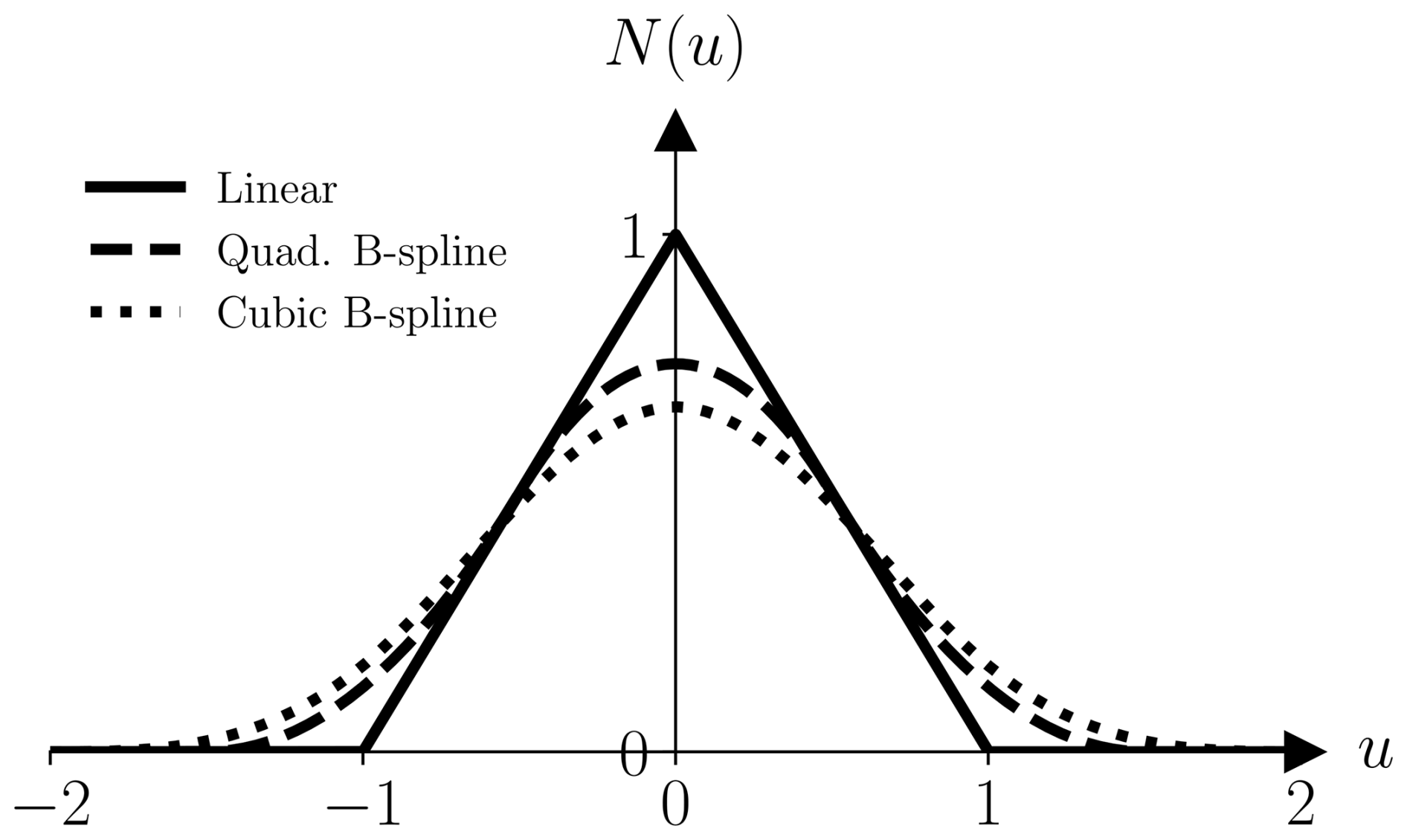
In order to overcome the so-called cell-crossing issues typically associated with the original formulation of MPM, Matter relies on B-spline interpolation functions as proposed by Steffen et al. (2008a). In particular, given a grid spacing Δx, the interpolation function between a grid node i and a particle p may be written

$$\begin{array}{}\text{(23)}& N_i\left({\mathit{x}}_p\right)=\prod _{\mathit{\alpha }=\mathrm{1}}^{d}N\left({\displaystyle \frac{x_{p\mathit{\alpha }}-x_{i\mathit{\alpha }}}{\mathrm{\Delta }x}}\right)\end{array}$$

where α denotes the component. Here, N(u) could, e.g., be the quadratic B-spline

$$\begin{array}{}\text{(24)}& N\left(u\right)=\left\{\begin{array}{ll}\frac{\mathrm{3}}{\mathrm{4}}-|u{|}^{\mathrm{2}},& \mathrm{if}\left|u\right|<\frac{\mathrm{1}}{\mathrm{2}}\\ \frac{\mathrm{1}}{\mathrm{2}}(\frac{\mathrm{3}}{\mathrm{2}}-|u|{)}^{\mathrm{2}},& \mathrm{if}\frac{\mathrm{1}}{\mathrm{2}}\le \left|u\right|<\frac{\mathrm{3}}{\mathrm{2}}\\ \mathrm{0},& \mathrm{otherwise}\end{array}\right.\end{array}$$

as illustrated in Fig. 2. As such, particles are influenced by grid nodes up until a distance 1.5Δx away. Higher-order B-splines are also considered, in particular cubic B-splines, which require an increased local support. Although cubic B-splines provide greater accuracy and smoothness within the interior domain and help mitigate numerical fracture, their performance near boundaries can degrade due to the increased local support required. Consequently, for simulations where near-boundary behavior is critical, quadratic B-splines may offer a more robust and reliable alternative. Other approaches used by the MPM community to suppress cell-crossing instabilities include the Generalized Interpolation Material Point Method (GIMP) (Bardenhagen and Kober, 2004) and Moving Least Square MPM (MLS-MPM) (Hu et al., 2018b).

Figure 2 Interpolation functions.

After distributing particles over the domain of the body, they are initiated with a mass m_p, an initial volume $V_p^{\mathrm{0}}$, an initial velocity ${\mathit{v}}_p^{\mathrm{0}}=\mathbf{0}$ (when initially at rest) and a deformation gradient ${\mathit{F}}_p^{\mathrm{0}}=\mathit{I}$ (when initially undeformed). Then, for each time step n of size Δt, the computational steps are outlined below, and a summary is presented in Algorithm 1.

Algorithm 1 An explicit B-spline (M)USL (A)PIC/(A)FLIP MPM scheme.

Initialize m_p, V_p, x_p according to material domain and density

Initialize v_p=0, F^E=I

For n=0, …, max time steps:

1. Initiate or adapt grid to material domain

2. Adapt time step: $\mathrm{\Delta }t=\min \left(C_{\mathrm{cfl}}\mathrm{\Delta }x/{max}_p\left|\right|{\mathit{v}}_p^{n+\mathrm{1}}|{|}_{L_{\mathrm{2}}},C_{\mathrm{elastic}}\mathrm{\Delta }x/\sqrt{E/\mathit{\rho }}\right)$

3. Interpolate particle mass and velocity to grid:

(a) $m_i^n=\sum _p{m}_p{N}_i\left({\mathit{x}}_p^n\right)$

EITHER (b) (if PIC/FLIP) ${\mathit{v}}_i^n=\frac{\mathrm{1}}{m_i^n}\sum _p{m}_p{\mathit{v}}_p^n{N}_i\left({\mathit{x}}_p^n\right)$

OR (c) (if APIC/AFLIP) ${\mathit{v}}_i^n=\frac{\mathrm{1}}{m_i^n}\sum _p{m}_p\left({\mathit{v}}_p^n+{\mathit{B}}_p^n{\mathit{D}}_p^{-\mathrm{1}}({\mathit{x}}_i^n-{\mathit{x}}_p^n)\right)N_i\left({\mathit{x}}_p^n\right)$

(d) (if MIBF, Sect. 4.3) ${\mathit{\mu }}_{b,i}^n=\frac{\mathrm{1}}{\sum _p{N}_i\left({\mathit{x}}_p^n\right)}\sum _p{\mathit{\mu }}_{m,p}{N}_i\left({\mathit{x}}_p^n\right)$

4. Update grid velocity: ${\mathit{v}}_i^{n+\mathrm{1}}={\mathit{v}}_i^n+\frac{\mathrm{\Delta }t}{m_i^n}{\mathit{f}}_i^n$ where ${\mathit{f}}_i^n=-\sum _p{V}_p^{\mathrm{0}}\frac{\partial \mathrm{\Psi }\left({\mathit{F}}^{E,n}\right)}{\partial {\mathit{F}}^E}\left({\mathit{F}}^{E,n}{)}^T\mathrm{\nabla }{N}_i\right({\mathit{x}}_p^n)+m_i^n\mathit{g}$ is the grid force

5. Apply boundary conditions on grid: e.g., ${\mathit{v}}_{i\in D}^{n+\mathrm{1}}=\mathrm{0}$ for non-slip

6. Update particle velocity:

(a) ${\mathit{v}}_p^{\mathrm{PIC}}=\sum _{i\in \mathrm{grid}}{\mathit{v}}_i^{n+\mathrm{1}}{N}_i\left({\mathit{x}}_p^n\right)$

(b)${\mathit{v}}_p^{\mathrm{FLIP}}={\mathit{v}}_p^n+\sum _{i\in \mathrm{grid}}({\mathit{v}}_i^{n+\mathrm{1}}-{\mathit{v}}_i^n)N_i\left({\mathit{x}}_p^n\right)$

(c) ${\mathit{v}}_p^{n+\mathrm{1}}=C_{\mathrm{transfer}}{\mathit{v}}_p^{\mathrm{FLIP}}+(\mathrm{1}-C_{\mathrm{transfer}}){\mathit{v}}_p^{\mathrm{PIC}}$

(d) (if APIC/AFLIP) ${\mathit{B}}_p^{n+\mathrm{1}}=\sum _{i\in \mathrm{grid}}{\mathit{v}}_i^{n+\mathrm{1}}({\mathit{x}}_i^n-{\mathit{x}}_p^n{)}^T{N}_i({\mathit{x}}_p^n)$

7. (If MUSL) revisit step 3 by interpolating ${\mathit{v}}_p^{n+\mathrm{1}}$ from step 4 to the grid, thus overwriting ${\mathit{v}}_i^{n+\mathrm{1}}$

8. Compute trial elastic strain:

(a) ${\mathit{F}}_p^{E,\mathrm{trial}}=\left(\mathit{I}+\mathrm{\Delta }t\sum _{i\in \mathrm{grid}}{\mathit{v}}_i^{n+\mathrm{1}}{\left(\mathrm{\nabla }{N}_i\left({\mathit{x}}_p^n\right)\right)}^T\right){\mathit{F}}_p^{E,n}$

(b) SVD of ${\mathit{F}}_p^{E,\mathrm{trial}}={\mathit{U}}_p^E{\mathbf{\Sigma }}_p^{E,\mathrm{trial}}({\mathit{V}}_p^E{)}^T$

(c) ${\mathit{\epsilon }}_p^{E,\mathrm{trial}}=\ln {\mathbf{\Sigma }}_p^{E,\mathrm{trial}}$

9. If $y\left(\mathit{\tau }\left({\mathit{\epsilon }}_p^{E,\mathrm{trial}}\right)\right)>\mathrm{0}$, perform return mapping: ${\mathit{\epsilon }}_p^{E,n+\mathrm{1}}=\mathrm{RM}({\mathit{\epsilon }}_p^{E,\mathrm{trial}},\mathrm{\dots })$ where RM is the return mapping and update elastic deformation gradient ${\mathit{F}}_p^{E,n+\mathrm{1}}={\mathit{U}}_p^E{e}^{{\mathit{\epsilon }}_p^{E,n+\mathrm{1}}}({\mathit{V}}_p^E{)}^T$, otherwise accept trial state.

10. Update positions: ${\mathit{x}}_p^{n+\mathrm{1}}={\mathit{x}}_p^n+\mathrm{\Delta }t{\mathit{v}}_p^{\mathrm{PIC}}$.

3.1 Step 1: initiate or adapt grid

A regular background Eulerian grid is adapted to cover the material domain by an excess given by the support of the chosen B-spline. Typically, the grid cell size Δx is chosen such that there are at least four and eight particles per grid cell in two and three spatial dimensions, respectively. In order to improve computational efficiency, the grid is expanded or contracted to only cover the material domain, keeping Δx constant with time.

3.2 Step 2: update size of time step

The size of the time step is adapted following the Courant–Friedrichs–Lewy (CFL) condition,

$$\begin{array}{}\text{(25)}& \mathrm{\Delta }t\le C_{\mathrm{cfl}}{\displaystyle \frac{\mathrm{\Delta }x}{\underset{p}{max}\left(\left|\right|{\mathit{v}}_p^{n+\mathrm{1}}|{|}_{L_{\mathrm{2}}}\right)}}\end{array}$$

and is at the same time restricted through the elastic wave speed such that

$$\begin{array}{}\text{(26)}& \mathrm{\Delta }t\le C_{\mathrm{elastic}}{\displaystyle \frac{\mathrm{\Delta }x}{\sqrt{E/\mathit{\rho }}}}\end{array}$$

where C_cfl≤1 and C_elastic≤1 are appropriate positive constants chosen to obtain a stable scheme.

3.3 Step 3: transfer mass and velocity from particles to grid

The mass and velocity on each grid node are determined by interpolating the masses and velocities of all particles within the support of the interpolation functions. The grid mass is calculated as

$$\begin{array}{}\text{(27)}& m_i^n=\sum _{p=\mathrm{1}}^{N_{\mathrm{particles}}}{m}_p{N}_i\left({\mathit{x}}_p^n\right).\end{array}$$

In the original formulation of MPM (using a PIC or FLIP scheme as will be explained further in Step 6), the grid velocity is

$$\begin{array}{}\text{(28)}& {\mathit{v}}_i^n={\displaystyle \frac{\mathrm{1}}{m_i^n}}\sum _{p=\mathrm{1}}^{N_{\mathrm{particles}}}{m}_p{\mathit{v}}_p^n{N}_i\left({\mathit{x}}_p^n\right)\end{array}$$

which preserves momentum. However, considering velocities as locally affine on each particle, transfer schemes that preserve affine velocity fields can be formulated where

$$\begin{array}{}\text{(29)}& {\mathit{v}}_i^n={\displaystyle \frac{\mathrm{1}}{m_i^n}}\sum _{p=\mathrm{1}}^{N_{\mathrm{particles}}}{m}_p\left({\mathit{v}}_p^n+{\mathit{G}}_p^n({\mathit{x}}_i^n-{\mathit{x}}_p^n)\right)N_i\left({\mathit{x}}_p^n\right)\end{array}$$

with ${\mathit{G}}_p={\mathit{B}}_p{\mathit{D}}_p^{-\mathrm{1}}$ similar to a velocity gradient where D_p is similar to an inertia tensor¹. It can be shown that D_p is approximately $\frac{\mathrm{1}}{\mathrm{4}}(\mathrm{\Delta }x{)}^{\mathrm{2}}\mathit{I}$ for a uniform grid using quadratic B-splines (Jiang et al., 2015; Nguyen et al., 2023).

3.4 Step 4: update grid velocity

Assuming a forward Euler time integration, the grid velocity at the next time step is

$$\begin{array}{}\text{(30)}& {\mathit{v}}_i^{n+\mathrm{1}}={\mathit{v}}_i^n+{\displaystyle \frac{\mathrm{\Delta }t}{m_i^n}}{\mathit{f}}_i^n\end{array}$$

where the grid forces are, using $\mathit{\tau }=\frac{\partial \widehat{\mathrm{\Psi }}\left({\mathit{\epsilon }}^E\right)}{\partial {\mathit{\epsilon }}^E}=\frac{\partial \mathrm{\Psi }\left({\mathit{F}}^E\right)}{\partial {\mathit{F}}^E}{{\mathit{F}}^E}^T$,

$$\begin{array}{}\text{(31)}& {\mathit{f}}_i^n=-\sum _{p=\mathrm{1}}^{N_{\mathrm{particles}}}{V}_p^{\mathrm{0}}{\displaystyle \frac{\partial \mathrm{\Psi }\left({\mathit{F}}^{E,n}\right)}{\partial {\mathit{F}}^E}}\left({\mathit{F}}^{E,n}{)}^T\mathrm{\nabla }{N}_i\right({\mathit{x}}_p^n)+m_i^n\mathit{g}\end{array}$$

where $V_p^{\mathrm{0}}$ is the initial particle volume.

3.5 Step 5: apply boundary conditions

Appropriate boundary conditions are enforced on grid velocities ${\mathit{v}}_{i\in D}^{n+\mathrm{1}}$ where i∈D denotes the set of grid points inside the domain D given by the level sets describing the objects/terrain. This is outlined in detail in Sect. 4.

3.6 Step 6: transfer grid velocity to particles

Define the particle velocities

$$\begin{array}{}\text{(32)}& {\displaystyle }& {\displaystyle }{\mathit{v}}_p^{\mathrm{PIC}}=\sum _{i\in \mathrm{grid}}{\mathit{v}}_i^{n+\mathrm{1}}{N}_i\left({\mathit{x}}_p^n\right),\text{(33)}& {\displaystyle }& {\displaystyle }{\mathit{v}}_p^{\mathrm{FLIP}}={\mathit{v}}_p^n+\sum _{i\in \mathrm{grid}}({\mathit{v}}_i^{n+\mathrm{1}}-{\mathit{v}}_i^n)N_i\left({\mathit{x}}_p^n\right).\end{array}$$

In a PIC scheme, the particle velocity at n+1 is taken as

$$\begin{array}{}\text{(34)}& {\mathit{v}}_p^{n+\mathrm{1}}={\mathit{v}}_p^{\mathrm{PIC}}\end{array}$$

while in a FLIP scheme

$$\begin{array}{}\text{(35)}& {\mathit{v}}_p^{n+\mathrm{1}}={\mathit{v}}_p^{\mathrm{FLIP}}.\end{array}$$

A highly dissipative scheme, PIC does not preserve angular momentum in the grid-to-particle transfer, leading to rotational artifacts. The FLIP scheme partly improves angular momentum conservation and reduces dissipation by only transferring the velocity increments. However, this may promote a more pronounced “ringing instability” (Love and Sulsky, 2006). Stomakhin et al. (2013) suggested a weighted combination of the PIC and FLIP transfer schemes, creating a trade-off between reducing dissipation associated with PIC on the one hand and suppressing instabilities associated with FLIP on the other hand. In such a PIC-FLIP scheme, the particle velocity at n+1 is taken as

$$\begin{array}{}\text{(36)}& {\displaystyle }{\mathit{v}}_p^{n+\mathrm{1}}& {\displaystyle }=C_{\mathrm{transfer}}{\mathit{v}}_p^{\mathrm{FLIP}}+(\mathrm{1}-C_{\mathrm{transfer}}){\mathit{v}}_p^{\mathrm{PIC}}\text{(37)}& {\displaystyle }& {\displaystyle }=\sum _{i\in \mathrm{grid}}{\mathit{v}}_i^{n+\mathrm{1}}{N}_i\left({\mathit{x}}_p^n\right)+C_{\mathrm{transfer}}({\mathit{v}}_p^n-\sum _{i\in \mathrm{grid}}{\mathit{v}}_i^n{N}_i({\mathit{x}}_p^n\left)\right)\end{array}$$

where $C_{\mathrm{transfer}}\in [\mathrm{0},\mathrm{1}]$ sets the PIC-FLIP combination ratio. Lower values of C_transfer result in more dissipation.

Later, affine PIC (APIC) was proposed by Jiang et al. (2015), conserving angular momentum in both transfers, thus resolving rotations. With a stability similar to PIC without massive dissipation, the dissipation of APIC is comparable to that of FLIP. In an APIC scheme, the particle velocity at n+1 follows Eq. (34) while the particle-to-grid transfer is accomplished through Eq. (29). Therefore, an update of B_p is also necessary, in particular,

$$\begin{array}{}\text{(38)}& {\mathit{B}}_p^{n+\mathrm{1}}=\sum _i{\mathit{v}}_i^{n+\mathrm{1}}({\mathit{x}}_i^n-{\mathit{x}}_p^n{)}^T{N}_i({\mathit{x}}_p^n).\end{array}$$

Recently, Fei et al. (2021) introduced AFLIP which reduces dissipation further. A generalization of APIC, this was based on following an analogous approach to how PIC was combined with FLIP. In this new transfer scheme, the grid-to-particle transfer can be written exactly as Eq. (36), and using Eq. (38) to update B_p. The parameter C_transfer now represents an APIC-AFLIP ratio, with C_transfer=0 meaning pure APIC and C_transfer=1 meaning pure AFLIP. A choice of C_transfer closer to unity significantly reduces dissipation compared to APIC.

Matter offers PIC, FLIP, APIC and AFLIP. In the context of USF MPM, these different transfer schemes have been critically compared in Duverger et al. (2024) to which the reader is referred for details. In general, the use of APIC is recommended due to its robustness and strong mathematical foundation, however, in highly dynamic and rate-dependent scenarios where numerical dissipation becomes significant, the AFLIP method is often preferred. Including the older transfer schemes, PIC and FLIP, allows for assessing the sensitivity of the problem to numerical dissipation, which can pose a challenge in MPM simulations. There exist also other recent transfer schemes, e.g., polynomial PIC (Fu et al., 2017), which is generalization of APIC using locally polynomial (as opposed to locally affine) approximations to the grid velocity field, and power PIC (Qu et al., 2022) based on the power particle idea of de Goes et al. (2015).

3.7 Step 7: re-interpolate grid velocities

When using MUSL (Sulsky et al., 1995) instead of USL, we must revisit Step 3 by interpolating ${\mathit{v}}_p^{n+\mathrm{1}}$ from Step 4 to the grid, thus overwriting ${\mathit{v}}_i^{n+\mathrm{1}}$. This is an optional step that may enhance the stability of the simulation.

3.8 Step 8: compute trial strain

In an “elastic predictor – plastic corrector” scheme, the deformation gradient is first updated in a trial step, assuming the body deforms purely elastically. In a forward Euler step, the trial step can be written as

$$\begin{array}{}\text{(39)}& {\displaystyle }{\mathit{F}}_p^{E,\mathrm{trial}}& {\displaystyle }={\mathit{F}}_p^{E,n}+\mathrm{\Delta }t\mathrm{\nabla }{\mathit{v}}^{n+\mathrm{1}}\left({\mathit{x}}_p\right){\mathit{F}}_p^{E,n}\text{(40)}& {\displaystyle }& {\displaystyle }=\left(\mathit{I}+\mathrm{\Delta }t\sum _{i\in \mathrm{grid}}{\mathit{v}}_i^{n+\mathrm{1}}{\left(\mathrm{\nabla }{N}_i\left({\mathit{x}}_p^n\right)\right)}^T\right){\mathit{F}}_p^{E,n}.\end{array}$$

The singular value decomposition of the trial elastic deformation gradient is

$$\begin{array}{}\text{(41)}& {\mathit{F}}_p^{E,\mathrm{trial}}={\mathit{U}}_p^{E,\mathrm{trial}}{\mathbf{\Sigma }}_p^{E,\mathrm{trial}}({\mathit{V}}_p^{E,\mathrm{trial}}{)}^T.\end{array}$$

Assume an elastic model based on Hencky strain is used such that the trial elastic Hencky strain is given by

$$\begin{array}{}\text{(42)}& {\mathit{\epsilon }}_p^{E,\mathrm{trial}}=\ln {\mathbf{\Sigma }}_p^{E,\mathrm{trial}}\end{array}$$

which from a computational perspective can be represented as a d-dimensional vector.

Figure 3 Compression of a cube of side length L with E=1 MPa and ν=0.3, using PIC-FLIP with C_transfer=0.99. (a) Stress-strain curve from finest discretization. (b) Convergence in the relative error of the measured bulk modulus K under finer discretization. Adapted from Blatny (2023).

3.9 Step 9: check yield criterion and return mapping

The Kirchhoff stress $\mathit{\tau }\left({\mathit{\epsilon }}_p^{E,\mathrm{trial}}\right)$ is calculated based on Hencky's elasticity model, and if the yield criterion is satisfied, then

$$\begin{array}{}\text{(43)}& {\mathit{F}}_p^{E,n+\mathrm{1}}={\mathit{F}}_p^{E,\mathrm{trial}}\mathrm{if}y\left(\mathit{\tau }\left({\mathit{\epsilon }}_p^{E,\mathrm{trial}}\right)\right)\le \mathrm{0}.\end{array}$$

On the other hand, if the yield criterion is not satisfied, plastic deformations occurred, and a projection to the yield surface must be made according to the plastic flow rule as

$$\begin{array}{}\text{(44)}& {\mathit{\epsilon }}_p^{E,n+\mathrm{1}}={\mathit{\epsilon }}_p^{E,\mathrm{trial}}-\mathrm{\Delta }t{\dot{\mathit{\gamma }}}_p^{n+\mathrm{1}}{\displaystyle \frac{\partial g\left(\mathit{\tau }\left({\mathit{\epsilon }}_p^{E,n+\mathrm{1}}\right)\right)}{\partial \mathit{\tau }}}\end{array}$$

which is given here as an implicit equation. If g is constant (e.g., perfect plasticity + associative plastic flow), this becomes a much simpler equation to solve. The elastic deformation gradient at n+1 is then obtained as

$$\begin{array}{}\text{(45)}& {\mathit{F}}_p^{E,n+\mathrm{1}}={\mathit{U}}_p^{E,\mathrm{trial}}{e}^{{\mathit{\epsilon }}_p^{E,n+\mathrm{1}}}{\left({\mathit{V}}_p^{E,\mathrm{trial}}\right)}^T.\end{array}$$

3.10 Step 10: update particle positions

The particle positions are updated according to

$$\begin{array}{}\text{(46)}& {\mathit{x}}_p^{n+\mathrm{1}}={\mathit{x}}_p^n+\mathrm{\Delta }t{\mathit{v}}_p^{\mathrm{PIC}}\end{array}$$

regardless of the choice of transfer scheme, whether that is PIC, FLIP, APIC or AFLIP.

4 Terrain and objects

Terrain and objects are described as level sets. This is similar to the treatment in e.g., Zhao et al. (2023a), although only objects with imposed movements are considered in the context of this work. The terrain and objects can either be analytically constructed or provided as .vdb files (OpenVDB, 2012). Analytically creating a terrain or an object requires defining two functions: (1) an “inside”-function which, given a point in space, checks if the point is inside the object, and (2) a “normal”-function which, given a point on the surface of the object, provides the outward unit normal vector at this point. This can be accomplished by deriving from the provided ObjectGeneral class. For the common problem of a finite and/or moving plate, a special ObjectPlate is available.

As mentioned in Sect. 3.5, boundary conditions are enforced on the grid velocities. Thus, every grid node found to be inside the level sets has its velocity altered according to the specified boundary condition. The different options are listed below.

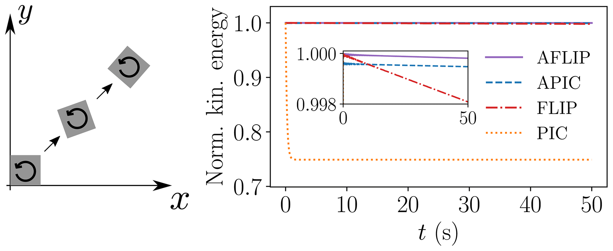
Figure 4 Elastic box with E=1 MPa and ν=0.3 undergoing rotation and translation. The normalized kinetic energy of the solid is plotted, using various particle-grid transfer schemes. Given an imposed initial angular velocity of 1 rad s⁻¹, the material has completed one rotation in 2π≈6 s. The inset plot is a zoomed view in order to distinguish FLIP, APIC and AFLIP.

4.1 No-slip

No-slip boundary conditions are realized by overwriting the grid velocities with the velocity of the object/terrain. In particular, in the case of a stationary object D, the grid nodes inside the D have their velocities updated as

$$\begin{array}{}\text{(47)}& {\mathit{v}}_{i\in D}^{n+\mathrm{1}}=\mathrm{0}.\end{array}$$

4.2 Frictional slip

Frictional slip can also be accomplished. As outlined in Blatny et al. (2024), an approximation to Coulomb's friction law on the grid velocities can be considered. Introducing a boundary friction parameter μ_b≥0, the velocity v relative to the boundary is obtained as

$$\begin{array}{}\text{(48)}& \begin{array}{rl}& {\mathit{v}}_{i\in D}^{n+\mathrm{1}}=\\ & \left\{\begin{array}{ll}{\mathit{v}}_T^{*}-{\mathit{\mu }}_b\left|\right|{\mathit{v}}_N^{*}|{|}_{L_{\mathrm{2}}}\frac{{\mathit{v}}_T^{*}}{\left|\right|{\mathit{v}}_T^{*}|{|}_{L_{\mathrm{2}}}}& \mathrm{if}\left|\right|{\mathit{v}}_T^{*}|{|}_{L_{\mathrm{2}}}>{\mathit{\mu }}_b|\left|{\mathit{v}}_N^{*}\right|{|}_{L_{\mathrm{2}}},\\ \mathbf{0}& \mathrm{otherwise}.\end{array}\right.\end{array}\end{array}$$

where v^* denotes the relative velocity (at time n+1) before the boundary condition is considered, and ${\mathit{v}}_T^{*}$ and ${\mathit{v}}_N^{*}$ are its tangential and normal components, respectively. In the special case μ_b=0, the tangential component of the relative velocity remains unchanged while the normal component vanishes. The boundary condition shown in Eq. (48) is typically only applied on grid nodes where ${\mathit{v}}_N^{*}$ indicates movement into the boundary such that the material can separate from the boundary.

Figure 5 Illustration of the influence of the particle-grid transfer scheme on the granular collapse. Here, all snapshots are taken at time t=0.22 s with $\mathrm{\Delta }{t}_{\mathrm{1}}=\mathrm{0.5}\mathrm{\Delta }x/\sqrt{E/\mathit{\rho }}$. Note that FLIP and AFLIP were used with C_transfer=0.99. Adapted from Blatny (2023).

4.3 Material-induced boundary friction (MIBF)

In the above situation, the boundary friction is constant in space and time, with μ_b being a parameter prescribed by the user. Consider an avalanche whose core is a dense granular flow well described by the μ(I)-rheology (see Sect. 2.8 and 2.9). In this situation, one might want the boundary friction to be given directly by the local value of the basal layer's varying (internal) friction μ, consequently giving the user one less parameter to prescribe. More generally, consider the situation where a non-constant material property μ_m, which may also depend on flow conditions, can be constructed. Such a spatiotemporal frictional boundary condition is accomplished in Matter by interpolating μ_m to the grid at every time step as shown in Step 3d in Algorithm 1. It is called Material-Induced Boundary Friction (MIBF) because the friction of the boundary is determined by a material property. If μ_m does not vary in time and space, MIBF reduces to the case of a constant boundary friction.

5 Verification tests

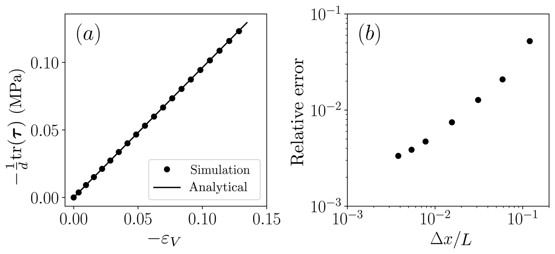
As a simple check of the finite strain elastic Hencky's model, consider here the compression of an elastic box. The volumetric Hencky strain ε_V=tr(ε) is measured, and according to Eq. (4), the relation $-\frac{\mathrm{1}}{d}\mathrm{tr}\left(\mathit{\tau }\right)=-K{\mathit{\epsilon }}_V$ should hold. Figure 3 shows that the measured stress response is consistent with the imposed elastic model and demonstrates convergence of the measured bulk modulus under finer discretization. For a more detailed analysis of the convergence properties of MPM, the reader is referred to, e.g., Steffen et al. (2008a, b). In particular, it should be noted that the introduction of boundaries, as was needed in this specific example to compress the material, may reduce the rate of convergence. In fact, this may be more pronounced with higher-order B-splines as these increase the local support of the interpolation, thus increasing the geometric error.

In order to evaluate the various particle-grid transfer schemes (PIC, FLIP, APIC, AFLIP) and to which extent they suffer from numerical dissipation, a simple problem of an elastic box undergoing translation and rotation in the absence of gravity is considered. This is sketched in Fig. 4 which also shows the evolution of the kinetic energy with time as the solid undergoes several rotations. Clearly, APIC and AFLIP conserve the kinetic energy well and much better than both PIC and FLIP, with AFLIP conserving the most energy. Notably, PIC suffers from severe dissipation and is unable to complete a full rotation, instead continuing only with translation corresponding to the drop in kinetic energy by 25 % shown in Fig. 4.

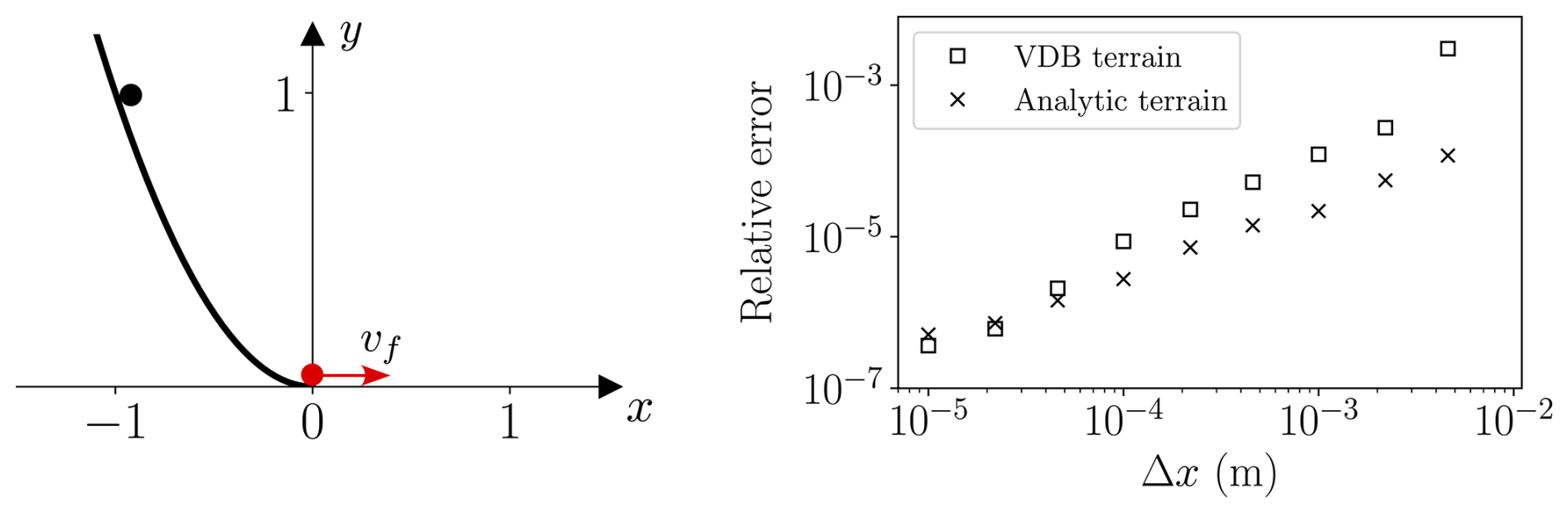
Figure 6 Verification of level set boundaries. A particle initially at rest at (−1, 1) is constrained to a frictionless boundary given by y=x². The relative error between the measured bottom velocity and the expected value $v_f=\sqrt{\mathrm{2}g}$ is plotted. Two different simulations are performed, one with an analytically specified level set and another with an OpenVDB level set.

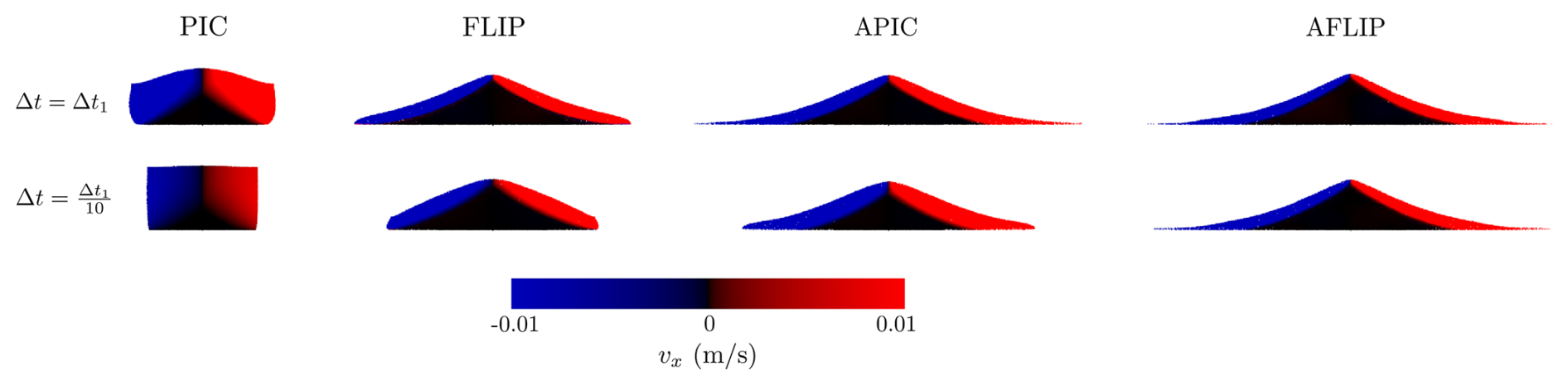
The above rotating box was a simple toy problem designed specifically to demonstrate the potentially severe effect of particle-grid transfer schemes in systems involving rotations. Choosing a minimally dissipative transfer scheme is especially important when modeling granular mechanics and flow problems as these are typically highly dynamic systems. Even in the relatively simple case of granular collapse under gravity, clear differences can be observed depending on the transfer scheme used, which is demonstrated in Fig. 5. This figure shows a collapse of a cohesionless Drucker-Prager granular material (see Sect. 2.5) at a specific time slightly before the material should come to rest on the horizontal non-slip surface. With a reasonable choice of Δt restricted by the elastic wave speed, it is observed that FLIP, APIC and AFLIP give approximately similar results, while PIC induces too much numerical dissipation resulting in a delayed and viscous response. If Δt is forced 10 times smaller, 10 times as many particle-grid transfers occur, thus inducing more numerical dissipation. In that case, it can be observed from the last row in Fig. 5 that only AFLIP is visually unaffected by this large increase in particle-grid transfers.

Various aspects of the implementation of the boundary conditions are checked in Figs. 6–8, respectively. Figure 6 shows that no significant differences between analytically specified level sets and OpenVDB level sets can be observed in this specific case of a particle following a frictionless parabola under gravity. In particular, both approaËches lead to second-order convergence under mesh refinement. In the case of frictional slip, Fig. 7 demonstrates that the material will slip if and only if θ>tan (μ_b). Furthermore, it confirms that the speed of the material sliding down various inclinations is consistent with the expected value from Coulomb's friction law. Figure 8 shows a particular variation of the setup described in the previous figure, where an artificially constructed material property μ_m=0.1t is used in the MIBF framework to provide a non-constant boundary friction μ_b. Although time is not a material property, such as, e.g., internal friction, this particular choice of a material property to use in MIBF allows for an analytical verification of its implementation.

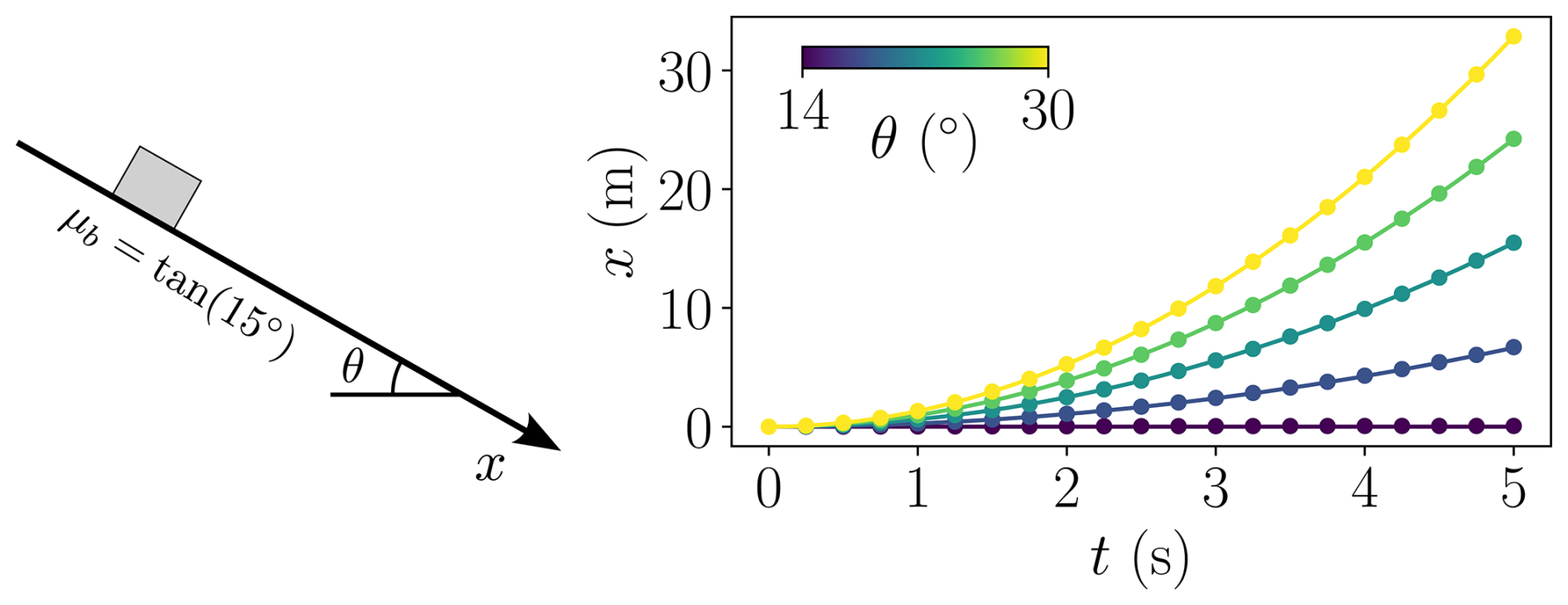
Figure 7 Verification of frictional boundary conditions. Mean position x (dots) of a stiff box sliding on a frictional plane with μ_b=tan(15°) on various inclinations θ. Analytical solutions (continuous lines) are given by $x=\max \left(\mathrm{0},\frac{\mathrm{1}}{\mathrm{2}}g\left(\sin \mathit{\theta }-{\mathit{\mu }}_b\cos \mathit{\theta }\right)t^{\mathrm{2}}\right)$.

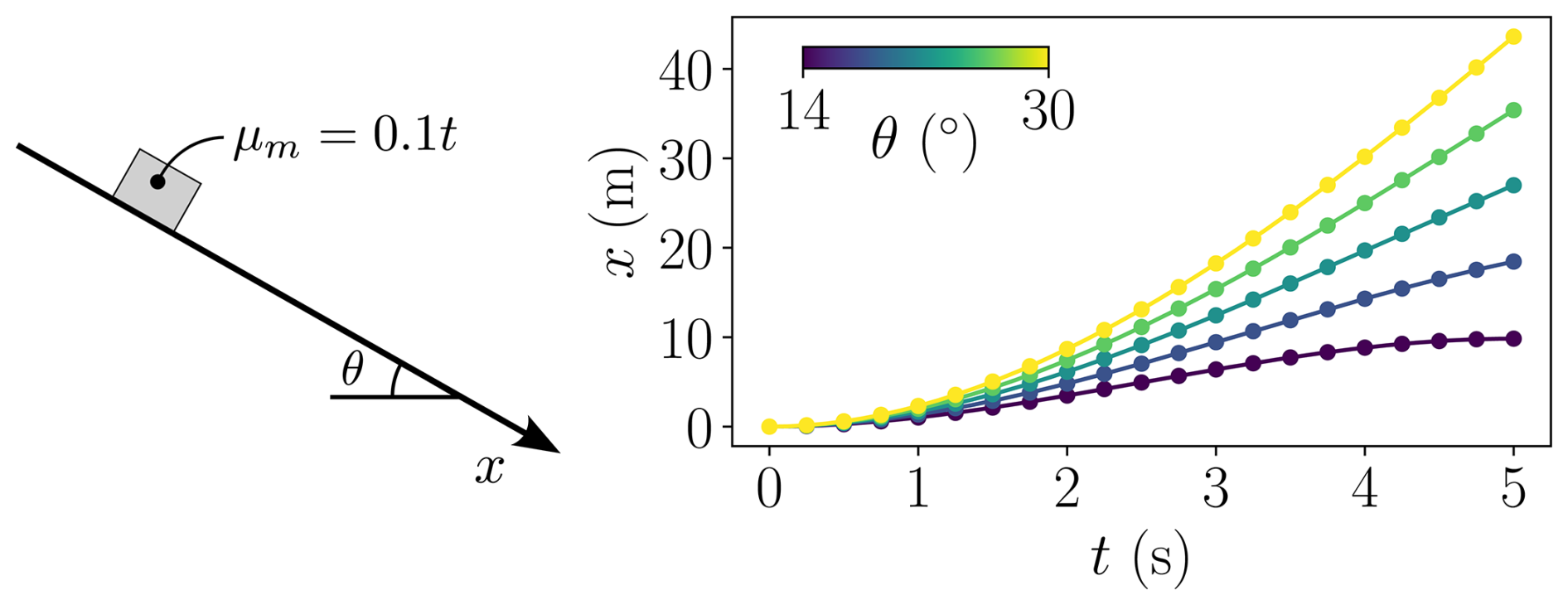
Figure 8 Verification of MIBF implementation. Same setup as Fig. 7, but now MIBF is used where μ_m=0.1t is given as an artificially constructed material property which at each time step is interpolated to the grid as shown in Step 3d in Algorithm 1. Analytical solutions (continuous lines) are given by $x=\max \left(\mathrm{0},\frac{\mathrm{1}}{\mathrm{2}}g(\sin \mathit{\theta }-\frac{\mathrm{1}}{\mathrm{3}}\mathrm{0.1}t\cos \mathit{\theta })t^{\mathrm{2}}\right)$.

6 Implementation, dependencies and performance

Matter is implemented in C$++$ and parallelized on shared memory using OpenMP (Dagum and Menon, 1998). The algorithm involves nested loops over particles and grid nodes. In order to reduce the computational complexity, these are generally implemented as outer loops over particles with the inner loop only summing over the grid nodes within the local support of the interpolation functions. Vectors and tensors are handled using the header-only linear algebra library Eigen (Gael and Benoit, 2010).

Depending on the problem at hand, the initial sampling of particle positions can affect the results. Regular sampling of the particles is generally discouraged as this may in some cases promote unwanted artifacts during deformation. To this end, Poisson disk distribution sampling (Bridson, 2007) is offered in Matter which relies on the single-header zero-dependencies implementation tph_poisson (Hinks, 2018). If using the provided particle sampling functions samplingParticles, the grid size Δx is determined to ensure a user-provided number of particles per grid cell (typically at least 4 in two dimensions and 8 in three dimensions). Particle data are saved at every chosen time frame as binary .ply files using the single-header zero-dependency code tinyply (Diakopoulos, 2018), In fact, the only required non-header-only dependency in addition to OpenMP is CMake (Hoffman, 2000). OpenVDB (OpenVDB, 2012) is only required in the case where an object or terrain level set is provided as a .vdb file. Such files may also be used to provide the level set which defines the domain of particle sampling. To this end, the samplingParticlesVdb function takes a .vdb file as input.

Table 1 Timing of a three-dimensional 0.1 m × 0.05 m × 0.1 m confined granular collapse, using E=1 MPa, ν=0.3 ρ=1000 kg m⁻³ and the cohesionless Drucker–Prager model (Sect. 2.5) with μ=0.58. The computation time is measured until t=0.4 s after equilibrium was reached. Initial discretization with 8 particles per grid cell volume Δx³. Using 8 threads in all cases, Computer A is a 2018 desktop workstation with Intel Xeon Gold 6136 CPUs with 192 GB RAM and Computer B is a 2023 Apple MacBook M3 laptop with 8 GB RAM.

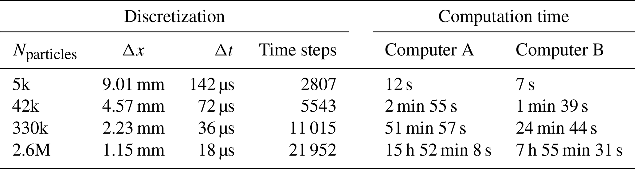
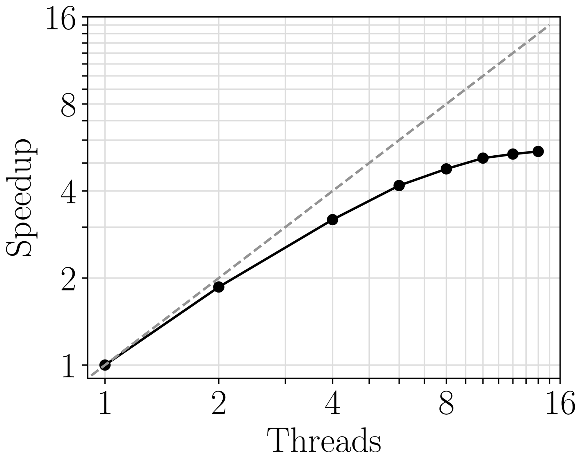
The implementation described above, along with the use of OpenVDB for complex terrain handling and OpenMP for shared-memory parallelization, contributes to the computational efficiency of the code. Table 1 lists some computation times for a granular collapse under gravity on a horizontal plane using an increasingly fine discretization. For the finest discretization (here 2.6 million particles), Fig. 9 shows the speedup with increasing threads, suggesting a max speedup of not more than 6. In comparison, de Vaucorbeil et al. (2021) reports speedups on Karamelo with shared-memory parallelization to around 8. Speedup may depend on the system and compiler, and a detailed analysis of this has not been conducted.

Figure 9 Speedup with number of threads in the simulation with 2.6M particles presented in last row in Table 1 using Computer A.

7 Examples

Figures 10–12 demonstrate some three-dimensional granular collapse and flow simulations using different constitutive models on small/simple and large/complex terrains. Figure 10 shows a cohesive granular collapse where the material is described by the Drucker–Prager model of Sect. 2.5. In addition to the tilted bottom plate, the collapse is restricted by a back wall and two side walls, all using the available plate objects described in Sect. 4. The material is visualized according to the plastic shear strain rate, highlighting the shear bands along which significant deformation occurs during the collapse. A similar visualization of the plastic shear strain rate is also used in Fig. 11 which shows granular flow through a silo where the material is described by the elastoplastic μ(I)-rheology of Sect. 2.8. Here, the silo is created analytically, specifically as a hyperbolic tangent curve $x=\tanh \left(y\right)+\mathrm{1}$ rotated along the vertical y-axis with a cut y=y_cut to define the silo opening through which the material flows. Using a mountain provided as a .vdb-file, Fig. 12 shows the flow of a material described by an overstress model (Sect. 2.7) with a Drucker–Prager yield. Enforcing MIBF, the non-constant internal friction is used as the basal friction. Notably, Fig. 12 also demonstrates that particle lift-off from the terrain is possible.

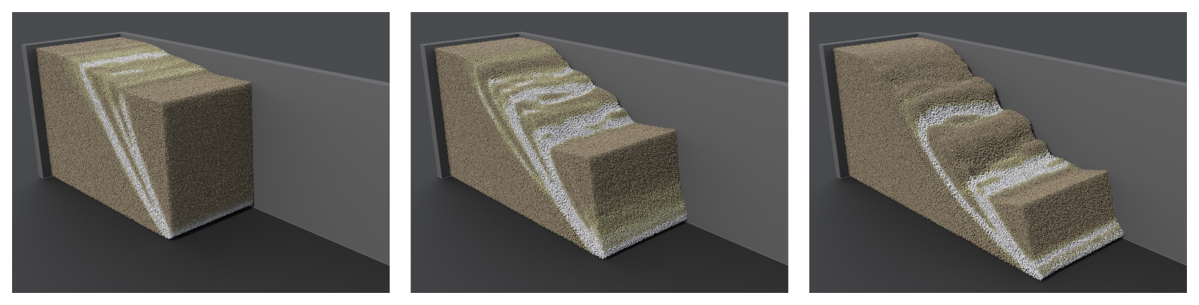
Figure 10 Three-dimensional cohesive granular collapse on a 10° tilted non-slip terrain using the cohesive Drucker-Prager model (μ=0.58 and q_c=100 Pa). The initial dimensions of the granular column was $\mathrm{20}\times \mathrm{14}\times \mathrm{10}$ cm, discretized with 1.6 million particles with initially 8 particles per grid cell. The displayed snapshots are taken at 0.1, 0.2 and 0.3 s, respectively, after release. Using 8 Intel Xeon Gold 6136 CPUs, the compute time between each of these snapshots were approximately 1 h and 10 min with Δt restricted by the choice of E=1 MPa and ρ=1000 kg m⁻³. The left side wall is not shown in order to visualize the material inside. The material is colored according to its plastic shear strain rate ${\dot{\mathit{\gamma }}}_S$, with brighter (whiter) colors representing higher strain rates, thus highlighting the shear bands.

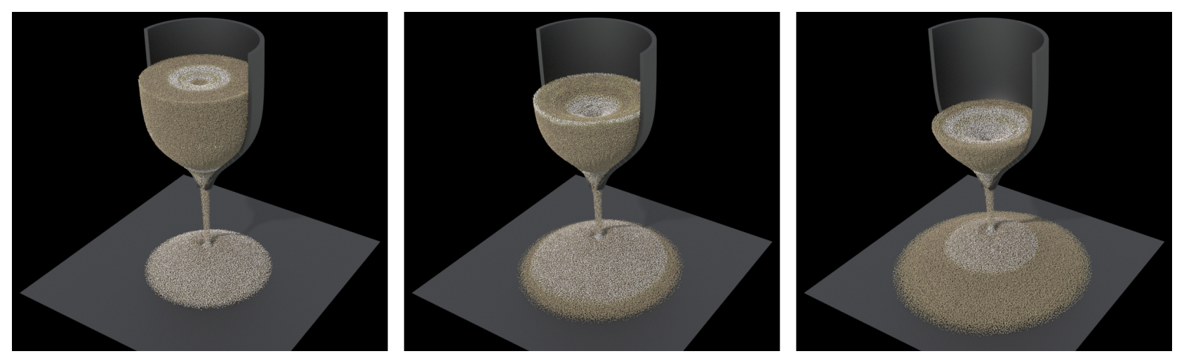
Figure 11 Three-dimensional flow from a silo using the elastoplastic μ(I)-rheology (μ₁=0.58, μ₂=0.84, ω=2.2 kg^−½ m^½). With a maximum radius of 2 m and height of 4 m, the silo is elevated 4 m above the ground where the deposit comes to rest. Only half of the silo boundary is shown. The displayed snapshots are taken at 50, 100 and 150 s, respectively, after release. With a discretization of 1 million particles, initially 8 particles per grid cell, running on 8 Intel Xeon Gold 6136 CPUs, the compute time between each snapshot was approximately 12 h with Δt restricted by the choice of E=1 MPa and ρ=1550 kg m⁻³. The material is colored according to its plastic shear strain rate ${\dot{\mathit{\gamma }}}_S$, with brighter (whiter) colors representing higher strain rates, thus highlighting the shear bands.

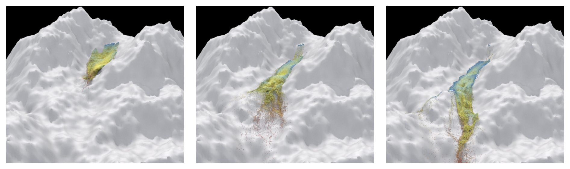
Figure 12 Three-dimensional flow on complex terrain with MIBF, using an overstress model with (t_visc=0.12 s, s=1) combined with a non-cohesive Drucker-Prager yield (μ=0.36). The displayed snapshots are taken at 6, 10 and 14 s, respectively, after release. Using 425k particles and Δx=0.43 m (with initially 8 particles per grid cell) the computation time from the leftmost to rightmost snapshot during 8 s was 47 min on 8 Intel Xeon Gold 6136 CPUs.

8 Concluding remarks

This article has presented Matter, an open-source MPM solver with a wide selection of elasto-viscoplastic models to describe the mechanics and rheology of granular media. The few cases presented in this article provide a glimpse into its capabilities in simulating granular media, from small-scale laboratory settings to flow on large-scale complex terrains. This includes terrains with various boundary conditions, including the proposed method of material-induced boundary friction. Built on a verified finite strain elastoplastic framework, Matter leverages recent advances in MPM particle-grid transfer schemes that reduce numerical dissipation.

The main limitations of the software should be highlighted. For example, modeling granular media immersed in or interacting with water or other fluids is beyond the scope of this software. Along these lines, the MPM community has proposed various strategies for handling multiple phases on one or more grids (e.g., Yerro et al., 2015; Higo et al., 2025), or proposed CFD coupling strategies (e.g., Higo et al., 2010; Tran et al., 2024). Moreover, including more than one type of material in the same simulation is currently not supported. Nevertheless, different constitutive parameters can be assigned to different particles with minimal modifications to the code. In addition, schemes to circumvent volumetric locking could also be considered in the future, in particular with the simple and elegant method of Zhao et al. (2023b). Although Matter represents a lightweight and efficient option for most problems that can be run on laptops and desktops, its current implementation is not optimized for sparse problems for which excessive simulation times can be witnessed. This could be addressed primarily by transitioning away from dense Eigen grids, however, the current strategy ensures a readable and adaptable code.

With the growing interest in understanding and modeling cohesive granular flow, particularly cohesive flows, this software aims to be a useful tool for both fundamental research and practical applications. This includes real-scale natural hazard applications, e.g., snow avalanches. While such mass movements are typically assessed with depth- or thickness-integrated models (Sampl and Zwinger, 2004; Christen et al., 2010; Tonnel et al., 2023), Matter represents an alternative three-dimensional approach to simulate these processes. Future developments aim to incorporate more advanced constitutive models for granular rheology, including non-local models, which are not yet considered. The community is also encouraged to contribute by integrating their own models into the framework.