ClimLoco1.0: CLimate variable confidence Interval of Multivariate Linear Observational COnstraint

Projections of future climate are key to society's adaptation and mitigation plans in response to climate change. Numerical climate models provide projections, but the large dispersion between them makes future climate very uncertain. To refine them, approaches called observational constraints (OCs) have been developed. They constrain an ensemble of climate projections using some real-world observations. However, there are many difficulties in dealing with the large literature on OC: the methods are diverse, the mathematical formulation and underlying assumptions are not always clear, and the methods are often limited to the use of the observations of only one variable. To address these challenges, this article proposes a new statistical model called ClimLoco1.0, which stands for “CLimate variable confidence Interval of Multivariate Linear Observational COnstraint”. It describes, in a rigorous way, the confidence interval of a projected variable (its best guess associated with an uncertainty at a confidence level) obtained using a multivariate linear OC. The article is built up in increasing complexity by expressing three different cases – the last one being ClimLoco1.0, the confidence interval of a projected variable: unconstrained, constrained by multiple real-world observations assumed to be noiseless, and constrained by multiple real-world observations assumed to be noisy. ClimLoco1.0 thus accounts for observational noise (instrumental error and climate-internal variability), which is sometimes neglected in the literature but is important as it reduces the impact of the OC. Furthermore, ClimLoco1.0 accounts for uncertainty rigorously by taking into account the quality of the estimators, which depends, for example, on the number of climate models considered. In addition to providing an interpretation of the mathematical results, this article proposes graphical interpretations based on synthetic data. ClimLoco1.0 is compared to some methods from the literature at the end of the article and is used in a real case study in the appendix.

1 Introduction

Numerical climate models are no exception to the often quoted statement “all models are wrong, but some are useful” from Box (1976). Indeed, their climate projections (simulated responses to a scenario of greenhouse gas and aerosol emissions) are useful to assess future climate change, but they vary widely from one climate model to another (e.g. Fig. 4.2 in IPCC in: Lee et al., 2021; Bellomo et al., 2021). There are now several dozen climate models around the world.

To assess the future value of a climate variable, such as global temperature in 2100, a traditional approach is to examine the distribution of projections of the variable simulated by an ensemble of climate models. The climate variable projected by climate models is hereafter referred to as the projected variable. The mean and standard deviation, which characterise the distribution of the projected variable, are usually used to define the so-called best guess and uncertainty of the projected variable, respectively (Collins et al., 2013). However, this uncertainty is generally high, and the best guess may be biased. To incorporate knowledge of real-world observations, statistical methods called observational constraints (OCs) or emergent constraints (Brunner et al., 2020a; O'Reilly et al., 2024) examine the distribution of the projected variable given real-world observations of an observable variable to obtain a constrained distribution. Such OC approaches are now used in the reports of the Intergovernmental Panel on Climate Change (IPCC) from 2021. They have huge implications for our society. The literature on OC methods is flourishing, but there are many difficulties in using them.

Firstly, the large number of existing OC methods makes it very difficult to choose one. Some methods average the projections of climate models, with weights that depend on the ability of the models to reproduce real-world observations of a given observable variable (Brunner et al., 2020; Giorgi and Mearns, 2002; Olson et al., 2018). Some methods use climate models to learn a relationship between the projected variable and a related observable variable and use this relationship and a real-world observation of that observable variable to predict the value of the projected variable. This relationship may be linear (Cox et al., 2018; Weijer et al., 2020; Bracegirdle and Stephenson, 2012; Karpechko et al., 2013) or non-linear (Schlund et al., 2020; Li et al., 2021; Forzieri et al., 2021). Other methods statistically provide the constrained distribution as the probability density function of the projected variable given the real-world observation of an observable variable (Bowman et al., 2018; Ribes et al., 2021). This diversity illustrates the lack of consensus on which approach to use. Methods are developed individually and need to be compared to better understand their differences and similarities, as done, for example, in Brunner et al. (2020a).

Secondly, the approaches and assumptions used to compute the constrained distribution can vary widely between articles and are not always reported. For example, their calculation does not always take into account the instrumental error associated with the real-world observation. Some papers provide clarification, e.g. Williamson and Sansom (2019), which proposed a comprehensive review of the underlying assumptions and uncertainty calculation in OC methods based on linear regression. However, some elements are still missing from the literature. For example, the terms “very likely”, “unlikely” etc. used by the IPCC (Mastrandrea et al., 2011) come from an underlying statistical model that provides a confidence interval, i.e. an interval that contains the projected variable value with a given confidence level. OC methods rarely use or describe a confidence interval. There is therefore a need for a proper statistical description of the theoretical basis of OCs, including confidence intervals, and a full description of the underlying statistical assumptions (Hegerl et al., 2021).

Thirdly, OC articles often use a univariate framework, i.e. they constrain the projected variable using only one observable variable. This may be surprising given the complexity of the climate system, which suggests that the spread between climate model projections may be related to multiple processes. For example, Cox et al. (2018) constrained the equilibrium climate sensitivity (ECS) using a measure of temperature variability. A few studies, particularly those using non-linear regression, employed a multivariate framework, but these are still rare. For example, Schlund et al. (2020) constrained future spatio-temporal gross primary production (GPP) by past spatio-temporal GPP and temperature.

To address these challenges, this article proposes a statistical model called ClimLoco1.0, which stands for “CLimate variable confidence Interval of Multivariate Linear Observational COnstraint”. ClimLoco1.0 expresses the confidence interval of a climate variable constrained using a linear multivariate observational constraint that takes into account observational noise. ClimLoco1.0 can also be used in univariate as well as multivariate form. This is the first version, 1.0, calling for further improvements to better account for all uncertainties. This article builds ClimLoco1.0 in progressively increasing complexity by expressing the confidence interval of the projected variable as (Sect. 2) unconstrained, (Sect. 3) as constrained by noiseless real-world observations, and (Sect. 4) as constrained by a noisy real-world observation, as represented in Fig. 1. The latter corresponds to ClimLoco1.0. Since the devil can be hidden in the details, the article presents the statistical procedure in a rigorous and clear manner, based on mathematical demonstrations. Moreover, the use of this complex statistical procedure is justified by illustrations of the underestimation of the uncertainty usually made in the literature by not using rigorous CIs. These results are then compared with some of the most widely used methods in the literature (Sect. 5): statistical methods as in Bowman et al. (2018) or Ribes et al. (2021) and methods based on linear regression as in Cox et al. (2018). Finally, the assumptions are summarised and discussed (Sect. 6).

In addition to providing the mathematical demonstrations, the appendices supply three valuable pieces of information. (i) A summary of the mathematical results in Tables A1 and A2. (ii) A section that explains all the key statistical concepts useful for understanding all the details of the article (Appendix B). (iii) A case study, illustrating the use of ClimLoco1.0 and testing its sensitivity to some parameters (Appendix I). The (Python) code and data that accompany the article are provided, as well as a user-friendly, simple example to replicate ClimLoco1.0.

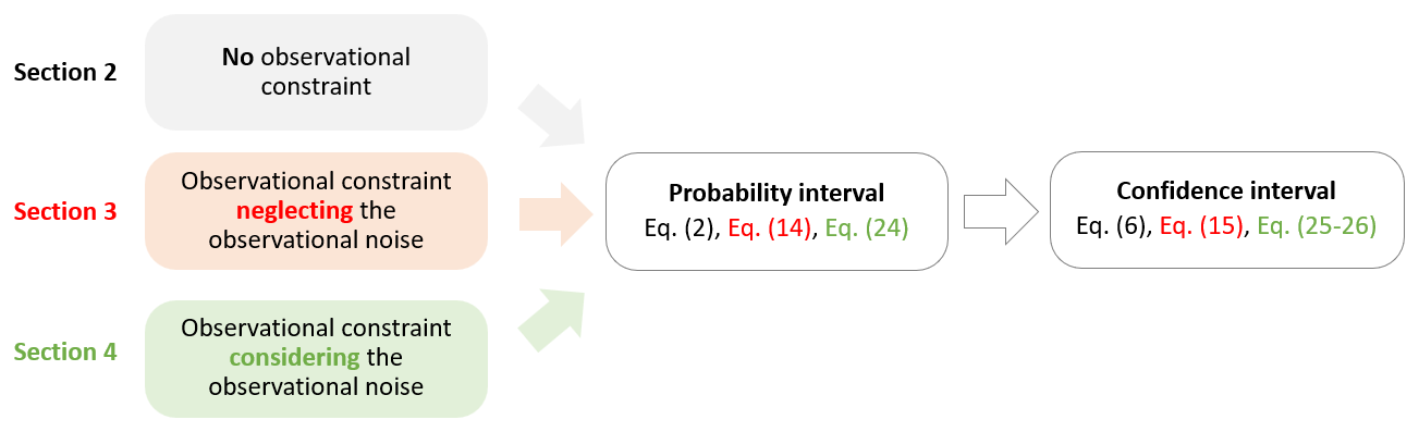
Figure 1 Flowchart of the study. ClimLoco1.0 is built in increasing complexity through three different sections: no observational constraint (OC), the OC neglecting the observational noise, and finally the OC considering the observational noise. Each section is also built in increasing complexity: neglecting the uncertainty due to the limited sample size (probability interval), then considering it (confidence interval).

2 Confidence interval of Y unconstrained

In order to anticipate society's adaptation and mitigation plans in response to climate change, it is necessary to estimate the value of a future variable called the projected variable and denoted Y, e.g. the global temperature in 2100. A common approach is to use an ensemble of climate model projections, e.g. CMIP6 (Coupled Model Intercomparison project version 6), which give different values of Y. Y is therefore a random variable; the dispersion between the climate model projections results from the randomness of Y.

To properly estimate the value of Y, this section defines the confidence interval (CI) of Y. It provides a best guess of Y value (centre of the interval) and an associated uncertainty (width of the interval) at a given confidence level. This section gradually builds up the CI of Y in increasing complexity. Firstly, it defines the probability interval (PI) of Y obtained assuming that the theoretical distribution of Y is known. Secondly, it defines the CI of Y obtained using this distribution estimated based on an ensemble of climate models. These two types of intervals are illustrated and interpreted using a synthetic example.

As stated above, the PI of Y is built using the theoretical distribution of Y. Here, this distribution is assumed to be Gaussian: $Y\sim \mathcal{N}({\mathit{\mu }}_Y,{\mathit{\sigma }}_Y^{\mathrm{2}})$, where μ_Y and ${\mathit{\sigma }}_Y^{\mathrm{2}}$ are respectively the expectation and variance of Y. The PI of Y is the interval that contains Y values with a probability of 1−α:

$$\begin{array}{}\text{(1)}& \mathrm{IP}\left({\mathit{\mu }}_Y-z{\mathit{\sigma }}_Y\le Y\le {\mathit{\mu }}_Y+z{\mathit{\sigma }}_Y\right)=\mathrm{1}-\mathit{\alpha },\end{array}$$

where z is the quantile of order $\mathrm{1}-\mathit{\alpha }/\mathrm{2}$ of a distribution 𝒩(0,1). For example, the 90 % PI (α=0.1) is obtained with z=1.65. In the IPCC, this 90 % probability corresponds to the term “very likely”, while “likely” stands for the 66 % probability, etc. The level of probability, i.e. 1−α, is a choice of the user. In the following, the PI of Y associated with a probability of 1−α described in Eq. (1) is denoted:

$$\begin{array}{}\text{(2)}& {\mathrm{PI}}_{\mathrm{1}-\mathit{\alpha }}\left(Y\right)=\left[{\mathit{\mu }}_Y\pm z{\mathit{\sigma }}_Y\right].\end{array}$$

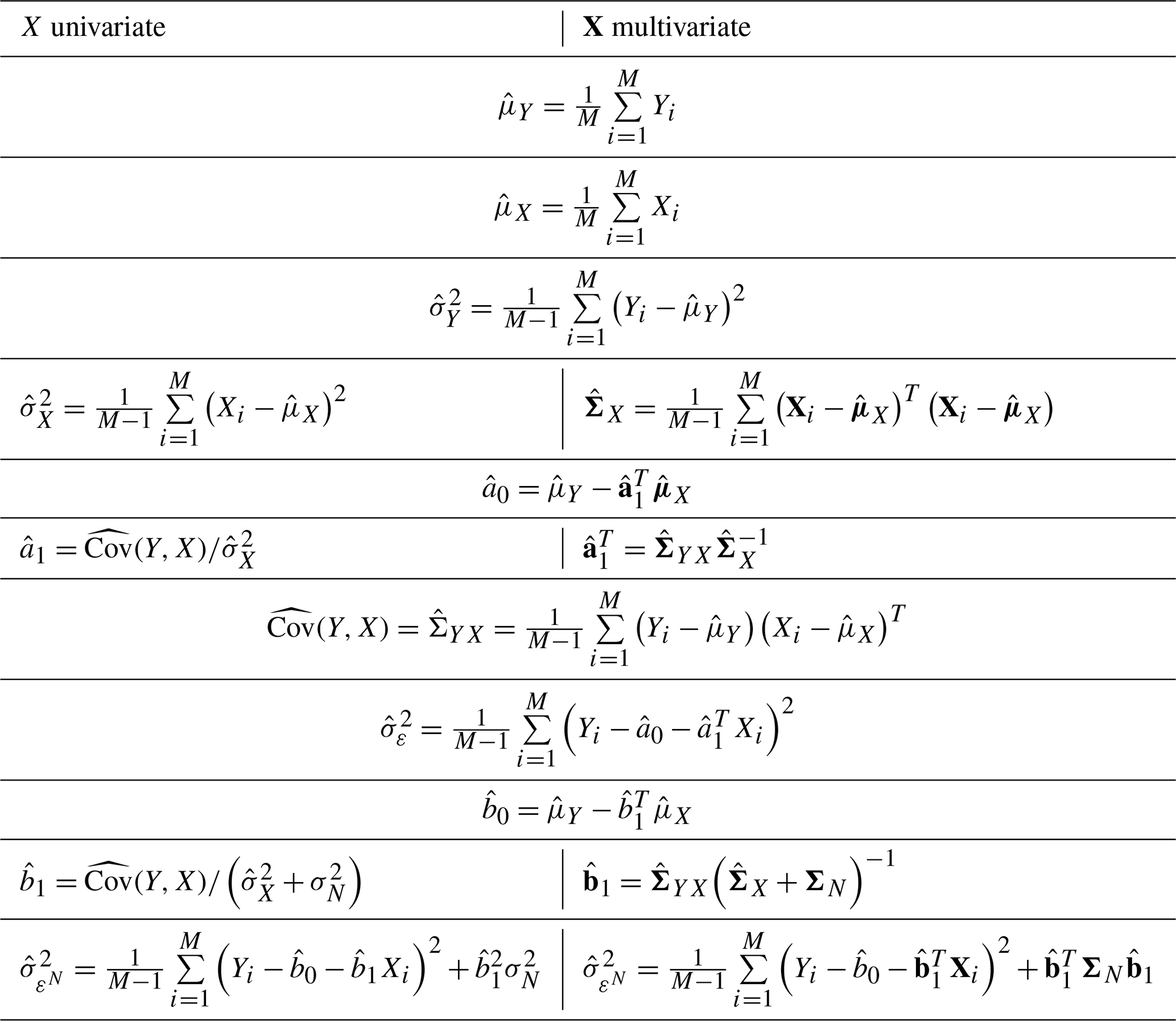
In fact, the expectation μ_Y and the standard deviation σ_Y are unknown. The PI described by Eq. (2) is therefore unknown. However, μ_Y and σ_Y can be estimated from an ensemble of climate model projections chosen by the user, for example, from CMIP6. This ensemble of M climate model projections yields a sample of M random variables, denoted (Y₁, …, Y_M). These random variables are assumed to be independent and to follow the same law as Y, which is assumed to be $\mathcal{N}({\mathit{\mu }}_Y,{\mathit{\sigma }}_Y^{\mathrm{2}})$. As a reminder, all the assumptions used in the article are summarised and discussed later in a dedicated section (Sect. 6). The classical estimators of the expectation μ_Y and variance ${\mathit{\sigma }}_Y^{\mathrm{2}}$ are:

$$\begin{array}{}\text{(3)}& {\displaystyle }& {\displaystyle }{\widehat{\mathit{\mu }}}_Y={\displaystyle \frac{\mathrm{1}}{M}}\sum _{i=\mathrm{1}}^M{Y}_i,\text{(4)}& {\displaystyle }& {\displaystyle }{\widehat{\mathit{\sigma }}}_Y^{\mathrm{2}}={\displaystyle \frac{\mathrm{1}}{M-\mathrm{1}}}\sum _{i=\mathrm{1}}^M{\left(Y_i-{\widehat{\mathit{\mu }}}_Y\right)}^{\mathrm{2}}.\end{array}$$

The literature usually replaces μ_Y and σ_Y with their estimators ${\widehat{\mathit{\mu }}}_Y$ and ${\widehat{\mathit{\sigma }}}_Y$ to estimate the PI [μ_Y±zσ_Y], which gives the interval [${\widehat{\mathit{\mu }}}_Y\pm z{\widehat{\mathit{\sigma }}}_Y$]. This interval has no clear statistical meaning. In fact, ${\widehat{\mathit{\mu }}}_Y$ and ${\widehat{\mathit{\sigma }}}_Y$ are random variables that depend on M, the number of climate models used. The quality of these two estimators affects the quality of the interval. It can be shown (see Appendix C) that using these estimators ${\widehat{\mathit{\mu }}}_Y$ and ${\widehat{\mathit{\sigma }}}_Y$, the values of Y are contained in the following interval with a probability of 1−α:

$$\begin{array}{}\text{(5)}& \begin{array}{rl}\mathrm{IP}& \left({\widehat{\mathit{\mu }}}_Y-t^{M-\mathrm{1}}{\widehat{\mathit{\sigma }}}_Y\sqrt{\mathrm{1}+{\displaystyle \frac{\mathrm{1}}{M}}}\le Y\le {\widehat{\mathit{\mu }}}_Y\right.\\ & \left.+t^{M-\mathrm{1}}{\widehat{\mathit{\sigma }}}_Y\sqrt{\mathrm{1}+{\displaystyle \frac{\mathrm{1}}{M}}}\right)=\mathrm{1}-\mathit{\alpha },\end{array}\end{array}$$

where t^M−1 is the quantile of a Student distribution with M−1 degrees of freedom associated with the probability 1−α. For example, with a confidence level of 90 % (α=0.1), t³⁰=1.70 and t⁵=2.02.

A subtle point is that this interval described in Eq. (5) is not a probability interval (PI) but a so-called confidence interval (CI). For example, the 90 % PI of Y is an interval that has a 90 % probability of containing Y values. It has deterministic bounds that frame a random variable. The CI of Y has random bounds, which also frame a random variable. In fact, the CI of Y described in Eq. (5) has random bounds because ${\widehat{\mathit{\mu }}}_Y$ and ${\widehat{\mathit{\sigma }}}_Y$ are random variables. Thus, different sample realisations, e.g. from different ensembles of climate models, will lead to different realisations of this CI. There is a confidence of 90 % that one realisation of the CI contains Y. In other words, out of 100 realisations of the 90 % CI, 90 should contain the value of the random variable Y. This is illustrated in Fig. 2, which shows 100 realisations of this CI of Y (error bars) at a 90 % confidence level, as well as 100 realisations of Y (red dots). This specific type of CI is also often called a prediction interval.

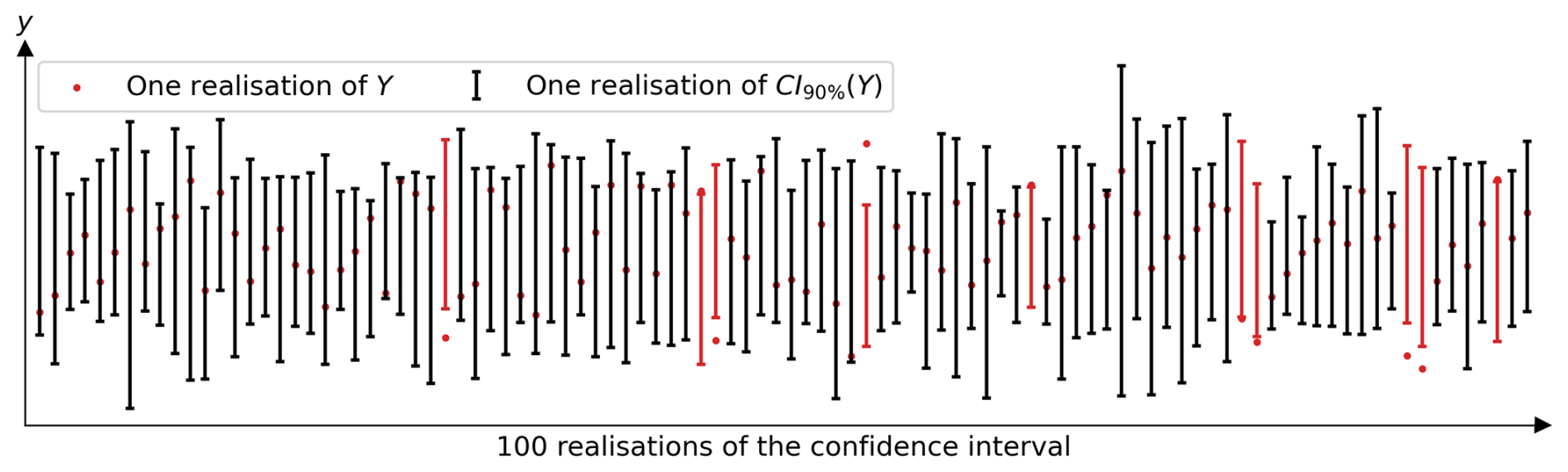
Figure 2 100 random realisations of the 90 % CI (confidence interval) of Y, CI_90 %(Y) described in Eq. (6), and 100 realisations of the random variable Y (red dots). Each realisation of the CI comes from a sample of M=10 random realisations of Y. Since the confidence level is 90 %, it is expected that 90 out of 100 CI realisations contain the realisation of Y, which is the case in this figure. The 10 CIs that did not contain the realisation of Y are shown in red.

The CI of Y associated with a confidence level of 1−α is then denoted:

$$\begin{array}{}\text{(6)}& {\mathrm{CI}}_{\mathrm{1}-\mathit{\alpha }}\left(Y\right)=\left[{\widehat{\mathit{\mu }}}_Y\pm t^{M-\mathrm{1}}{\widehat{\mathit{\sigma }}}_Y\sqrt{\mathrm{1}+{\displaystyle \frac{\mathrm{1}}{M}}}\right].\end{array}$$

Now that the CI of Y is defined, it allows us to study the effect of the number of climate models considered (M) on this CI. Throughout the paper, the same synthetic example is used, defined in Appendix D. It provides the theoretical PI of Y, which is unknown in reality and estimated by the CI of Y. It also provides one realisation of the CI of Y using a small (M=5) sample (Y₁, …, Y_M), and another using a large sample (M=30). These different samples can, for example, represent different ensembles of climate models (CMIP5, CMIP6, HighResMIP, …). Figure 3 shows the probability interval of Y, PI_1−α(Y) defined in Eq. (2), and the realisations of the two CI of Y (M=5 and M=30), CI_1−α(Y) defined in Eq. (6). In reality, the PI is unknown. This synthetic example allows us to compare the estimates with the truth.

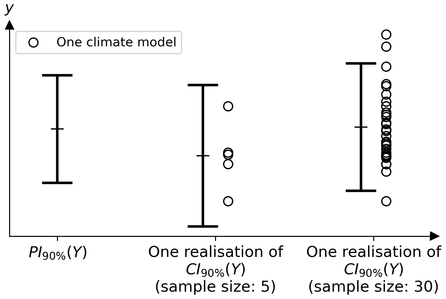
Figure 3 Synthetic example comparing the 90 % PI (probability interval) of Y (left), described in Eq. (2), with two realisations of the 90 % CI (confidence interval) of Y (middle and right), described in Eq. (6). The first realisation is obtained from the small sample of M=5 climate models, while the second is obtained from the large sample of M=30. We compare the realisations of CI with the PI, the truth that is unknown in reality. The details of the data simulation are given in Appendix D.

There are two important remarks about the CI of Y described in Eq. (6). Firstly, it converges in probability to the PI of Y described in Eq. (2) as M, the number of climate models considered, increases. Indeed, as M becomes large, the estimates ${\widehat{\mathit{\mu }}}_Y$ and ${\widehat{\mathit{\sigma }}}_Y$ (Eqs. 3 and 4) converge (in probability) to μ_Y and σ_Y, and the Student quantile converges to a Gaussian quantile. This is illustrated in Fig. 3, by comparing the PI of Y (left error bar) with the realisations of the CI of Y (middle and right error bars). Indeed, the large sample gives a CI of Y (right interval, at $\mathrm{CI}=[\mathrm{0.1}\pm \mathrm{1.9}]$) closer to the PI of Y (left interval, at $\mathrm{PI}=[\mathrm{0}\pm \mathrm{1.6}]$) than the small sample (middle interval, at $\mathrm{CI}=[-\mathrm{0.8}\pm \mathrm{2.2}]$). To accurately estimate both the centre and the width of the CI of Y, which represent the best guess and the uncertainty, respectively, it is therefore necessary to have as large a sample as possible. Secondly, the fewer the models, the larger the CI of Y. It is intuitive that estimating the CI of Y with less data will give a more uncertain result. Indeed, in Eq. (6), the terms t^M−1 and $\sqrt{\mathrm{1}+\frac{\mathrm{1}}{M}}$ are larger when M is smaller. These two aspects highlight the importance of having as many climate models as possible. However, the climate models considered must be independent, and the simulated variables must follow the same distribution as the real variables – two assumptions necessary for the calculation that are not fully satisfied (Knutti et al., 2017).

In the literature, the PI of Y, i.e. [μ_Y±zσ_Y], is often estimated as the empirical interval [${\widehat{\mathit{\mu }}}_Y\pm z{\widehat{\mathit{\sigma }}}_Y$]. However, as seen previously, this interval has no statistical basis, whereas CI${}_{\mathrm{1}-\mathit{\alpha }}\left(Y\right)=\left[{\widehat{\mathit{\mu }}}_Y\pm t^{M-\mathrm{1}}{\widehat{\mathit{\sigma }}}_Y\sqrt{\mathrm{1}+\frac{\mathrm{1}}{M}}\right]$ contains Y values with a given probability. The relative error of the interval width caused by using the wrong interval [${\widehat{\mathit{\mu }}}_Y\pm z{\widehat{\mathit{\sigma }}}_Y$] instead of the CI is therefore quantified as relative error in the width of this wrong interval (zσ_Y) compared to the width of the CI $\left(t^{M-\mathrm{1}}{\widehat{\mathit{\sigma }}}_Y\sqrt{\mathrm{1}+\frac{\mathrm{1}}{M}}\right)$:

$$\begin{array}{}\text{(7)}& E_{\mathrm{1}}={\displaystyle \frac{\left|z-t^{M-\mathrm{1}}\sqrt{\mathrm{1}+\frac{\mathrm{1}}{M}}\right|}{t^{M-\mathrm{1}}\sqrt{\mathrm{1}+\frac{\mathrm{1}}{M}}}}.\end{array}$$

This relative error, which depends on the sample size (M) and the confidence level (1−α) controlling z and t, is plotted as a function of these two parameters in Fig. 4. For typical sample sizes of ensembles of climate models, between 5 and 50, the relative error is between 3 % and 30 %. For example, with a confidence level of 68 % (z=1, “likely” in IPCC language) and a sample size of 20 climate models, the relative error is 5 %. Since the width of the interval represents the uncertainty, this means that the uncertainty is underestimated by 5 %, which is even higher for smaller sample sizes or higher confidence levels. This highlights the importance of using the rigorous formula provided in this article to express uncertainty more accurately.

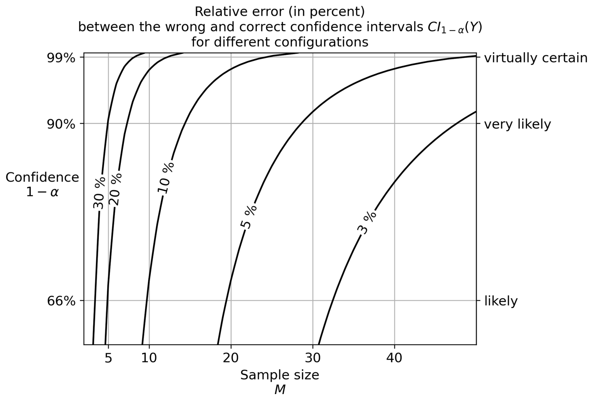
Figure 4 Uncertainty quantification errors caused by using the wrong interval instead of the correct one, that is, $\left[{\widehat{\mathit{\mu }}}_Y\pm z{\widehat{\mathit{\sigma }}}_Y\right]$ instead of $\left[{\widehat{\mathit{\mu }}}_Y\pm t^{M-\mathrm{1}}{\widehat{\mathit{\sigma }}}_Y\sqrt{\mathrm{1}+\frac{\mathrm{1}}{M}}\right]$. This relative error is described in Eq. (7). The contours correspond to relative errors of 30 %, 20 %, 10 %, 5 %, and 3 %.

Without even mentioning observational constraints, this section provides statistically sound formulae for estimating an interval that contains the value of a future variable from the projections of an ensemble of M climate models at a given confidence level, using confidence intervals. This brings a rigorous insight to climate science, where the simple mean and standard deviation are commonly used. The next part applies the same methodology to a linear observational constraint.

3 Confidence interval of Y constrained by a noiseless observation

Observational constraint (OC) methods have been developed to estimate more accurately the value of a projected variable Y. These methods “constrain” the distribution of Y by a “real-world” observation, denoted x₀, of an observable variable X. X has to be chosen by the user, as well as the observational dataset providing x₀. In this section, the real-world observation is assumed to be noiseless (no observational noise, e.g. due to instrumental errors). This assumption is relaxed in the next section which defines ClimLoco1.0. The general formulation presented in this article can be applied to the choice of any arbitrary variables X and Y. The variable Y constrained by the observation x₀ of X is written as $Y|X=x_{\mathrm{0}}$.

As mentioned in the Introduction, many articles in the literature use univariate OCs, i.e. only one observable variable X is used to constrain Y. This can be very limiting, especially when Y depends on many processes, which is often the case in climate science. Therefore, an important contribution of this article is to give the formulation in a multivariate form, i.e. X∈ℝ^p with p the number of observable variables. However, for the sake of clarity, only the results for the univariate formulations are presented in the main part of the article. The multivariate formulations are given in Table A1.

This section gradually builds up the CI of $Y|X=x_{\mathrm{0}}$ in increasing complexity. Firstly, it defines the probability interval (PI) of Y built using the theoretical distribution of $Y|X=x_{\mathrm{0}}$ by assuming that this distribution is known. Secondly, it defines the CI of $Y|X=x_{\mathrm{0}}$ obtained using this distribution estimated based on an ensemble of climate models. These two types of intervals are illustrated and interpreted using a synthetic example.

As stated above, the PI of $Y|X=x_{\mathrm{0}}$ is build using the theoretical distribution of $Y|X=x_{\mathrm{0}}$. Here, this distribution is assumed to be Gaussian: $Y|X=x_{\mathrm{0}}\sim \mathcal{N}({\mathit{\mu }}_{Y|X=x_{\mathrm{0}}},{\mathit{\sigma }}_{Y|X=x_{\mathrm{0}}}^{\mathrm{2}})$, where ${\mathit{\mu }}_{Y|X=x_{\mathrm{0}}}$ and ${\mathit{\sigma }}_{Y|X=x_{\mathrm{0}}}^{\mathrm{2}}$ are, respectively, the expectation and variance of $Y|X=x_{\mathrm{0}}$. In the following, the PI of $Y|X=x_{\mathrm{0}}$ associated with a probability of 1−α is denoted as:

$$\begin{array}{}\text{(8)}& {\mathrm{PI}}_{\mathrm{1}-\mathit{\alpha }}\left(Y|X=x_{\mathrm{0}}\right)=\left[{\mathit{\mu }}_{Y|X=x_{\mathrm{0}}}\pm z{\mathit{\sigma }}_{Y|X=x_{\mathrm{0}}}\right],\end{array}$$

where z is the quantile of order $\mathrm{1}-\mathit{\alpha }/\mathrm{2}$ of a distribution 𝒩(0,1). In order to express the terms ${\mathit{\mu }}_{Y|X=x_{\mathrm{0}}}$ and ${\mathit{\sigma }}_{Y|X=x_{\mathrm{0}}}^{\mathrm{2}}$ in Eq. (8), a linear regression framework is used:

$$\begin{array}{}\text{(9)}& \begin{array}{rl}Y=& \mathbb{E}\left[Y\right|X]+\mathit{\epsilon },\\ & \mathrm{where}\mathbb{E}\left[Y\right|X]=a_{\mathrm{0}}+a_{\mathrm{1}}X,\mathit{\epsilon }\sim \mathcal{N}\left(\mathrm{0},{\mathit{\sigma }}_{\mathit{\epsilon }}\right).\end{array}\end{array}$$

The coefficients a₀ and a₁ are the intercept and the slope of the linear regression of Y on X, respectively, and ε is a random variable representing the regression error with σ_ε its standard deviation. Using this linear regression model, it can be shown (see the proof in Appendix E) that the terms ${\mathit{\mu }}_{Y|X=x_{\mathrm{0}}}$ and ${\mathit{\sigma }}_{Y|X=x_{\mathrm{0}}}^{\mathrm{2}}$ can be expressed as:

$$\begin{array}{}\text{(10)}& {\displaystyle }& {\displaystyle }{\mathit{\mu }}_{Y|X=x_{\mathrm{0}}}=a_{\mathrm{0}}+a_{\mathrm{1}}{x}_{\mathrm{0}}\text{(11)}& {\displaystyle }& {\displaystyle }={\mathit{\mu }}_Y+\mathit{\rho }{\displaystyle \frac{{\mathit{\sigma }}_Y}{{\mathit{\sigma }}_X}}\left(x_{\mathrm{0}}-{\mathit{\mu }}_X\right),\text{(12)}& {\displaystyle }& {\displaystyle }{\mathit{\sigma }}_{Y|X=x_{\mathrm{0}}}^{\mathrm{2}}={\mathit{\sigma }}_{\mathit{\epsilon }}^{\mathrm{2}}\text{(13)}& {\displaystyle }& {\displaystyle }=\left(\mathrm{1}-{\mathit{\rho }}^{\mathrm{2}}\right){\mathit{\sigma }}_Y^{\mathrm{2}},\end{array}$$

where μ_X and μ_Y are the expectations of X and Y, σ_X and σ_Y are the standard deviations of X and Y, and ρ is the linear correlation between X and Y. The PI of Y constrained by X=x₀ described by Eq. (8) can then be rewritten as:

$$\begin{array}{}\text{(14)}& {\mathrm{PI}}_{\mathrm{1}-\mathit{\alpha }}\left(Y|X=x_{\mathrm{0}}\right)=\left[a_{\mathrm{0}}+a_{\mathrm{1}}{x}_{\mathrm{0}}\pm z{\mathit{\sigma }}_{\mathit{\epsilon }}\right].\end{array}$$

To illustrate this, the same synthetic case study as before is used, detailed in Appendix D. The PI of Y constrained is shown in Fig. 5a and b (in red) and is compared with the PI of Y unconstrained (in black) in Fig. 5b. The constraint on Y has two effects: (a) it changes the best guess (centre of the interval) and (b) it reduces the uncertainty (width of the interval).

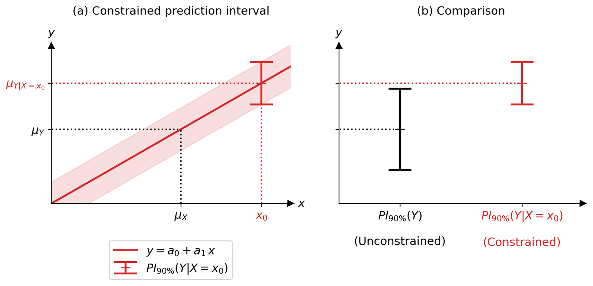
Figure 5 (a) Example showing the 90 % probability interval (PI) of the projected variable Y constrained by the observation x₀ of an observable variable X, as described by Eq. (14). (b) Comparison between the 90 % PI of Y constrained (red) and unconstrained (black) as described by Eqs. (14) and (2), respectively. The values of means, variances, etc. are given in Appendix D.

• a.

  When Y is constrained ($\mathrm{PI}\left(Y\right|X=x_{\mathrm{0}})$), it has a different best guess (centre of interval) than when it is unconstrained (PI(Y)). We interpret this in two different ways, using Eqs. (10) and (11). The first equation gives a graphical interpretation: the constrained expectation of Y is directly the real-world observation fed into the regression. This is illustrated in Fig. 5a. The second equation is useful to understand the correction between the best guess of Y constrained and unconstrained: ${\mathit{\mu }}_{Y|X=x_{\mathrm{0}}}-{\mathit{\mu }}_Y=\mathit{\rho }\frac{{\mathit{\sigma }}_Y}{{\mathit{\sigma }}_X}(x_{\mathrm{0}}-{\mathit{\mu }}_X)$. It depends on two terms: the regression slope $\mathit{\rho }\frac{{\mathit{\sigma }}_Y}{{\mathit{\sigma }}_X}$, which depends in particular on the correlation between X and Y, and the difference between the real-world observation and the theoretical centre of the climate models distribution on X. It is called here (x₀−μ_X) the theoretical multi-model bias. In other words, the constrained best guess of Y (${\mathit{\mu }}_{Y|X=x_{\mathrm{0}}}$) is a corrected version on the unconstrained best guess of Y (μ_Y), knowing the theoretical multi-model bias of X (x₀−μ_X) and the relationship between X and Y $\left(\mathit{\rho }\frac{{\mathit{\sigma }}_Y}{{\mathit{\sigma }}_X}\right)$. In the example of Fig. 5a, there is a positive theoretical multi-model bias associated with a positive relationship between X and Y, thus a correction to a higher best guess (${\mathit{\mu }}_{Y|X=x_{\mathrm{0}}}>{\mathit{\mu }}_Y$). Observational constraints are generally used to reduce uncertainty, but the correction of the best guess between constrained and unconstrained is very important and should not be forgotten, as it allows for correcting the multi-model bias.

• b.

  When Y is constrained, it has a lower uncertainty (width of $\mathrm{PI}\left(Y\right|X=x_{\mathrm{0}})$) than when it is unconstrained (width of PI(Y)). We interpret this in two different ways, using Eqs. (12) and (13). Equation (12) provides a graphical interpretation: the uncertainty of Y when constrained is directly the regression error. The 90 % regression error is represented by the red tube in Fig. 5a. Equation (13) expresses the variance of $Y|X=x_{\mathrm{0}}$ as the variance of Y multiplied by 1−ρ², which is between 0 and 1. The uncertainty of Y constrained by observation is therefore smaller than the uncertainty of Y unconstrained: this is the desired reduction in uncertainty. The stronger the correlation between X and Y, the greater the reduction in uncertainty. In the example shown in Fig. 5b, the strong correlation (0.85) between X and Y reduces the uncertainty well; the red interval is narrower than the black one.

The use of the PI of Y constrained, Eq. (14), requires knowledge of the theoretical parameters a₀, a₁, and σ_ε, which are unknown in reality. To estimate them, an ensemble of M climate models chosen by the user, e.g. CMIP6, HighResMIP, (etc.) is used. It is written (X₁, Y₁), …, (X_M, Y_M) as a sample of M pairs of random variables (X, Y). They are assumed to be independent and to follow the same law as (X, Y), which is assumed to be bivariate Gaussian. This sample allows to define the estimators ${\widehat{a}}_{\mathrm{0}}$, ${\widehat{a}}_{\mathrm{1}}$, and ${\widehat{\mathit{\sigma }}}_{\mathit{\epsilon }}$ of a₀, a₁, and σ_ε (see formulas in Table A2). To estimate $\mathrm{PI}\left(Y\right|X=x_{\mathrm{0}})$, one may want to replace the theoretical parameters by the estimated ones, which gives the following interval: $\left[{\widehat{a}}_{\mathrm{0}}+{\widehat{a}}_{\mathrm{1}}{x}_{\mathrm{0}}\pm z{\widehat{\mathit{\sigma }}}_{\mathit{\epsilon }}\right]$. However, as seen in the previous section, this interval has no statistical meaning. Instead, it is shown in Appendix F that the estimated parameters lead to the following confidence interval (CI) of $Y|X=x_{\mathrm{0}}$:

$$\begin{array}{}\text{(15)}& \begin{array}{rl}{\mathrm{CI}}_{\mathrm{1}-\mathit{\alpha }}\left(Y|X=x_{\mathrm{0}}\right)& =\left[{\widehat{a}}_{\mathrm{0}}+{\widehat{a}}_{\mathrm{1}}{x}_{\mathrm{0}}\right.\\ & \left.\pm t^{M-\mathrm{2}}{\widehat{\mathit{\sigma }}}_{\mathit{\epsilon }}\sqrt{\mathrm{1}+{\displaystyle \frac{\mathrm{1}}{M}}+{\displaystyle \frac{{\left(x_{\mathrm{0}}-{\widehat{\mathit{\mu }}}_X\right)}^{\mathrm{2}}}{M{\widehat{\mathit{\sigma }}}_X^{\mathrm{2}}}}}\right].\end{array}\end{array}$$

The corresponding expression when X is multivariate is given in Table A1. The definitions of the estimators are provided in Table A2.

To illustrate these mathematical results, Fig. 6 uses the same synthetic case study as before. It shows the realisations of two samples (X₁, Y₁), …, (X_M, Y_M): one of size M=5 and the other of size M=30. The realisation of each sample corresponds to each row. As shown in Fig. 6a, these two different sample realisations lead to two different realisations of the estimated linear relationship $y={\widehat{a}}_{\mathrm{0}}+{\widehat{a}}_{\mathrm{1}}x$ (red line) and the constrained confidence intervals (red interval). The red shading represents the ${\mathrm{CI}}_{\mathrm{90}\mathit{\%}}\left(Y\right|X=x_{\mathrm{0}})$ obtained for different positions of the observation x₀. Figure 6b compares the realisations of the CI of Y unconstrained CI_90 %(Y) and constrained ${\mathrm{CI}}_{\mathrm{90}\mathit{\%}}\left(Y\right|X=x_{\mathrm{0}})$ and the PI of Y constrained ${\mathrm{PI}}_{\mathrm{90}\mathit{\%}}\left(Y\right|X=x_{\mathrm{0}})$.

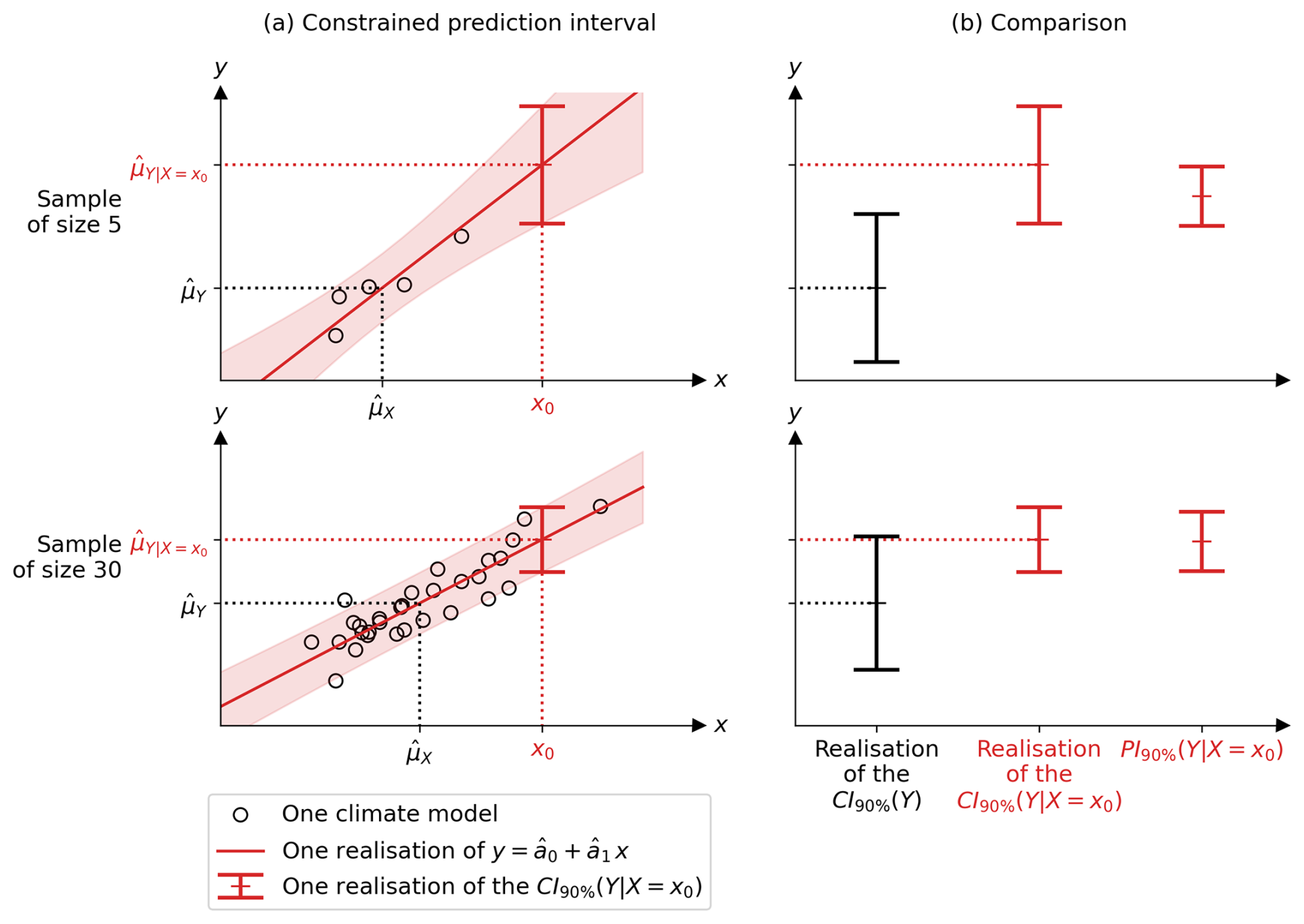
Figure 6 Synthetic example showing (a) the first column, two realisations of the 90 % confidence interval (CI) of Y constrained by the observation x₀ of X, described in Eq. (15). The two realisations come from two different samples (X₁, Y₁), …, (X_M, Y_M) of size M=5 and M=30 (black circles) and correspond to the two rows of the figure. The estimated linear regression and its 90 % error are shown as the red line and shading, respectively. (b) The second column compares, in red, the confidence (middle) and probability (right) intervals of the constrained Y. The larger sample (second row) gives a better CI than the smaller one (first row), which is closer to the PI. Panel (b) also compares the CI of Y constrained (middle) and unconstrained (left, in black). The details of the data simulation are given in Appendix D. ${\widehat{\mathit{\mu }}}_X$ and ${\widehat{\mathit{\mu }}}_Y$ are the unconstrained means of X and Y, while ${\widehat{\mathit{\mu }}}_{Y|X=x_{\mathrm{0}}}$ is the constrained mean of Y. The observation x₀ is assumed to be noiseless.

On the one hand, there are two similarities between the CI of Y constrained ($Y|X=x_{\mathrm{0}}$) and unconstrained (Y). Firstly, the CI of Y constrained described by Eq. (15) converges (in probability) to the PI of Y constrained described by Eq. (8) as the sample size M increases. Consequently, the CI obtained from a large sample (second panel) is closer to the PI than the one obtained from a small sample (first panel), as shown in Fig. 6b. Secondly, the CI of $Y|X=x_{\mathrm{0}}$ is larger when the sample size M is smaller, due to the term $t^{M-\mathrm{2}}\sqrt{\mathrm{1}+\frac{\mathrm{1}}{M}+\frac{(x_{\mathrm{0}}-{\widehat{\mathit{\mu }}}_X{)}^{\mathrm{2}}}{M{\widehat{\mathit{\sigma }}}_X^{\mathrm{2}}}}$ in Eq. (15). To summarise these two similarities between the unconstrained and constrained cases: a larger sample leads to a more correct and precise estimate of Y.

On the other hand, there are two important differences between the CI of Y constrained and unconstrained. Firstly, the centre of the $\mathrm{CI}\left(Y\right|X=x_{\mathrm{0}})$ is the observation fed into the regression, as described in Eq. (15). Using the previous equations, the difference between the centre (best guess) of the CI of Y constrained and unconstrained can be expressed as ${\widehat{\mathit{\mu }}}_{Y|X=x_{\mathrm{0}}}-{\widehat{\mathit{\mu }}}_Y={\widehat{a}}_{\mathrm{1}}(x_{\mathrm{0}}-{\widehat{\mathit{\mu }}}_X)$. This correction of the best guess depends on the estimated slope between X and Y, ${\widehat{a}}_{\mathrm{1}}$, and on what is called here the multi-model mean bias at X, $(x_{\mathrm{0}}-{\widehat{\mathit{\mu }}}_X)$. In other words, the constraint corrects the multi-model bias on Y, knowing the multi-model bias on X and the relationship between X and Y. This is illustrated in Fig. 6. Secondly, there is a difference in the square root term between the CI of Y constrained and unconstrained. The CI of Y constrained is larger by the amount $(x_{\mathrm{0}}-{\widehat{\mathit{\mu }}}_X{)}^{\mathrm{2}}/M{\widehat{\mathit{\sigma }}}_X^{\mathrm{2}}$. If the observation is far from the samples, this quantity is large, which makes the interval width (uncertainty) larger. In other words, the linear relationship is more uncertain away from the samples, in unknown territory. Furthermore, the latter term is multiplied by $\mathrm{1}/M$, which means that the linear relationship is more certain when obtained from a large sample size. This is illustrated in Fig. 6a on the small sample (first row): the constrained confidence interval grows rapidly as one moves away from the samples (black circles).

In summary, the equations and figures show the two benefits of OC: there is a correction to the best guess and a reduction in uncertainty, between the CI of Y unconstrained and constrained. To maximise the reduction in uncertainty, there is a need for as many (independent) climate models as possible.

As seen previously, to get a real estimate of the PI of Y constrained, namely [$a_{\mathrm{0}}+a_{\mathrm{1}}{x}_{\mathrm{0}}\pm z{\mathit{\sigma }}_{\mathit{\epsilon }}$], the correct approach is to use the CI of Y constrained, namely $\left[{\widehat{a}}_{\mathrm{0}}+{\widehat{a}}_{\mathrm{1}}{x}_{\mathrm{0}}\pm t^{M-\mathrm{2}}{\widehat{\mathit{\sigma }}}_{\mathit{\epsilon }}\sqrt{\mathrm{1}+\frac{\mathrm{1}}{M}+\frac{{\left(x_{\mathrm{0}}-{\widehat{\mathit{\mu }}}_X\right)}^{\mathrm{2}}}{M{\widehat{\mathit{\sigma }}}_X^{\mathrm{2}}}}\right]$. However, the literature sometimes uses [${\widehat{a}}_{\mathrm{0}}{\widehat{a}}_{\mathrm{1}}{x}_{\mathrm{0}}\pm z{\widehat{\mathit{\sigma }}}_{\mathit{\epsilon }}$], which has no statistical basis. The relative error in the interval width caused by using the wrong one instead of the correct one is therefore quantified as:

$$\begin{array}{}\text{(16)}& E_{\mathrm{2}}={\displaystyle \frac{\left|z-t^{M-\mathrm{2}}\sqrt{\mathrm{1}+\frac{\mathrm{1}}{M}+\frac{{\left(x_{\mathrm{0}}-{\widehat{\mathit{\mu }}}_X\right)}^{\mathrm{2}}}{M{\widehat{\mathit{\sigma }}}_X^{\mathrm{2}}}}\right|}{t^{M-\mathrm{2}}\sqrt{\mathrm{1}+\frac{\mathrm{1}}{M}+\frac{{\left(x_{\mathrm{0}}-{\widehat{\mathit{\mu }}}_X\right)}^{\mathrm{2}}}{M{\widehat{\mathit{\sigma }}}_X^{\mathrm{2}}}}}}.\end{array}$$

This relative error described by Eq. (16) depends on three parameters: (i) the sample size, M, (ii) the confidence level, 1−α, which controls z and t, and (iii) the standardised real-world observation, $\frac{{\left(x_{\mathrm{0}}-{\widehat{\mathit{\mu }}}_X\right)}^{\mathrm{2}}}{{\widehat{\mathit{\sigma }}}_X^{\mathrm{2}}}$. The relative error is shown in Fig. 7 for a fixed confidence level of 68 %, as a function of M (x-axis) and $\frac{{\left(x_{\mathrm{0}}-{\widehat{\mathit{\mu }}}_X\right)}^{\mathrm{2}}}{{\widehat{\mathit{\sigma }}}_X^{\mathrm{2}}}$ (y-axis). With a typical sample size of climate model ensembles between 5 and 50, the relative error is between 3 % and 30 %. In other words, using the wrong interval instead of the correct one implies an underestimation of the uncertainty between 3 % and 30 %. For example, using an ensemble of M=20 climate models, the error starts at 5 % and can easily exceed 10% if the observation is far from the ensemble of climate models (y-axis). This highlights the need to rigorously consider the performance of the estimators in order to correctly estimate the uncertainty using the rigorous CI defined in this article.

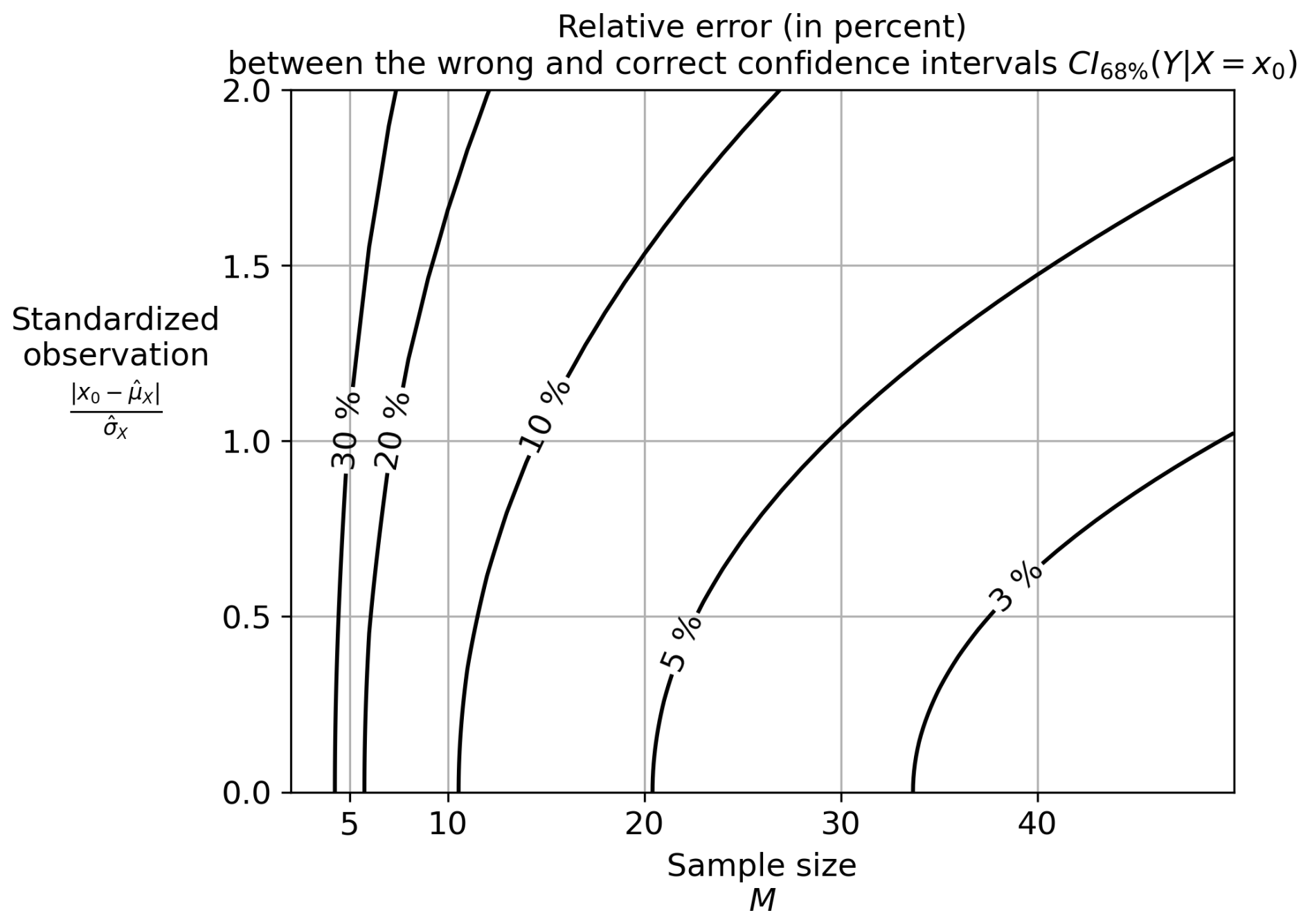
Figure 7 Uncertainty quantification error when constraining Y by using the wrong interval instead of the correct one, that is, $\left[{\widehat{a}}_{\mathrm{0}}+{\widehat{a}}_{\mathrm{1}}{x}_{\mathrm{0}}\pm z{\widehat{\mathit{\sigma }}}_{\mathit{\epsilon }}\right]$ instead of $\left[{\widehat{a}}_{\mathrm{0}}+{\widehat{a}}_{\mathrm{1}}^T{x}_{\mathrm{0}}\pm t^{M-\mathrm{2}}{\widehat{\mathit{\sigma }}}_{\mathit{\epsilon }}\sqrt{\mathrm{1}+\frac{\mathrm{1}}{M}+\frac{{\left(x_{\mathrm{0}}-{\widehat{\mathit{\mu }}}_X\right)}^{\mathrm{2}}}{M{\widehat{\mathit{\sigma }}}_X^{\mathrm{2}}}}\right]$. This error is described in Eq. (16). The error values are shown by the contours ranging from 3 % to 30 %. They are given as a function of the sample size (x-axis) and the distance between the observation and the multi-model ensemble. The confidence level is fixed at 68 % (i.e. z=1), a value often used in the literature.

4 ClimLoco1.0

The previous results were obtained under the assumption that the real-world observation x₀ is not noisy. In reality, x₀ is affected by observational noise, which is taken into account in this section, inspired by the theory of measurement error models (Fuller, 2009). Some papers define observational noise as internal variability (e.g. Brunner et al., 2020), others as measurement error (e.g. Hall et al., 2019), and others as both (e.g. Ribes et al., 2021). We argue here that both internal variability and measurement error should be taken into account, as both affect the real-world observation. Let X^N be the noisy version of X, linked by the noise model defined in Bowman et al. (2018):

$$\begin{array}{}\text{(17)}& X^N=X+N,\mathrm{with}N\sim \mathcal{N}\left(\mathrm{0},{\mathit{\sigma }}_N^{\mathrm{2}}\right)\mathrm{and}N⟂⟂X,\end{array}$$

where N is a random variable representing the observation noise, assumed to be Gaussian, centred, and independent of X. Its variance ${\mathit{\sigma }}_N^{\mathrm{2}}$ is assumed to be known. The projected variable Y constrained by the observation $x_{\mathrm{0}}^N$ of X^N affected by the observation noise is denoted $Y|X^N=x_{\mathrm{0}}^N$.

This section constructs ClimLoco1.0, which is the confidence interval of $Y|X^N=x_{\mathrm{0}}^N$, in increasing complexity, following the same steps as in the previous two sections. Firstly, it defines the probability interval (PI) of $Y|X^N=x_{\mathrm{0}}^N$ obtained using the theoretical distribution of $Y|X^N=x_{\mathrm{0}}^N$ by assuming that the distribution of $Y|X^N=x_{\mathrm{0}}^N$ is known. Secondly, it defines the CI of $Y|X^N=x_{\mathrm{0}}^N$ obtained using this distribution estimated based on an ensemble of climate models. These two types of intervals are illustrated and interpreted using a synthetic example. These different steps that construct ClimLoco1.0 are crucial to define and understand with rigour the best guess and uncertainty of any variable constrained by a noisy observation.

As stated above, the PI of $Y|X^N=x_{\mathrm{0}}^N$ is built using the theoretical distribution of $Y|X^N=x_{\mathrm{0}}^N$. Here, this distribution is assumed to be Gaussian: $Y|X^N=x_{\mathrm{0}}^N\sim \mathcal{N}({\mathit{\mu }}_{Y|X^N=x_{\mathrm{0}}^N}$, ${\mathit{\sigma }}_{Y|X^N=x_{\mathrm{0}}^N}^{\mathrm{2}})$, where ${\mathit{\mu }}_{Y|X^N=x_{\mathrm{0}}^N}$ and ${\mathit{\sigma }}_{Y|X^N=x_{\mathrm{0}}^N}^{\mathrm{2}}$ are, respectively, the expectation and variance of $Y|X^N=x_{\mathrm{0}}^N$. The following interval is the PI of $Y|X^N=x_{\mathrm{0}}^N$, i.e. it contains $Y|X^N=x_{\mathrm{0}}^N$ values with a probability of 1−α:

$$\begin{array}{}\text{(18)}& {\mathrm{PI}}_{\mathrm{1}-\mathit{\alpha }}\left(Y|X^N=x_{\mathrm{0}}^N\right)=\left[{\mathit{\mu }}_{Y|X^N=x_{\mathrm{0}}^N}\pm z{\mathit{\sigma }}_{Y|X^N=x_{\mathrm{0}}^N}\right],\end{array}$$

where z is the quantile of order $\mathrm{1}-\mathit{\alpha }/\mathrm{2}$ of a distribution 𝒩(0,1). This interval contains realisations of Y with a given confidence 1−α controlling z. To express the parameters ${\mathit{\mu }}_{Y|X^N=x_{\mathrm{0}}^N}$ and ${\mathit{\sigma }}_{Y|X^N=x_{\mathrm{0}}^N}^{\mathrm{2}}$, a linear regression framework is used, as in the previous section:

$$\begin{array}{}\text{(19)}& \begin{array}{rl}Y& =\mathbb{E}\left[Y\right|X^N]+{\mathit{\epsilon }}^N,\\ & \mathrm{where}\mathbb{E}\left[Y\right|X^N]=b_{\mathrm{0}}+b_{\mathrm{1}}{X}^N,{\mathit{\epsilon }}^N\sim \mathcal{N}\left(\mathrm{0},{\mathit{\sigma }}_{{\mathit{\epsilon }}^N}\right),\end{array}\end{array}$$

and where b₀ and b₁ are the intercept and slope of the linear model, respectively, and ε^N is a random variable representing the regression error with ${\mathit{\sigma }}_{{\mathit{\epsilon }}^N}$ its standard deviation. This linear regression is the regression of Y on X^N. However, climate models do not suffer from observational noise (instrumental error and internal variability): they provide realisations of X, not X^N. In fact, climate models do not suffer from instrumental error, but they can be affected by internal variability. However, the impact of internal variability can be reduced, for example, by averaging the members of a given climate model (different realisations run from different initial conditions). As climate models provide realisations of X and not X^N, it can be difficult to express the linear coefficients b₀ and b₁. However, using the model noise described by Eq. (17), which relates X^N to X, it is possible to obtain the expressions of b₀ and b₁ and hence the expression of ${\mathit{\mu }}_{Y|X^N=x_{\mathrm{0}}^N}$ and ${\mathit{\sigma }}_{Y|X^N=x_{\mathrm{0}}^N}^{\mathrm{2}}$. In fact, it can be shown (see Appendix G) that:

$$\begin{array}{}\text{(20)}& {\displaystyle }& {\displaystyle }{\mathit{\mu }}_{Y|X^N=x_{\mathrm{0}}^N}=b_{\mathrm{0}}+b_{\mathrm{1}}{x}_{\mathrm{0}}^N\text{(21)}& {\displaystyle }& {\displaystyle }={\mathit{\mu }}_Y+\mathit{\rho }{\displaystyle \frac{{\mathit{\sigma }}_Y}{{\mathit{\sigma }}_X}}{\displaystyle \frac{\mathrm{1}}{\mathrm{1}+\mathrm{1}/{\mathrm{SNR}}^{\mathrm{2}}}}\left(x_{\mathrm{0}}^N-{\mathit{\mu }}_X\right),\text{(22)}& {\displaystyle }& {\displaystyle }{\mathit{\sigma }}_{Y|X^N=x_{\mathrm{0}}^N}^{\mathrm{2}}={\mathit{\sigma }}_{{\mathit{\epsilon }}^N}^{\mathrm{2}}\text{(23)}& {\displaystyle }& {\displaystyle }=\left(\mathrm{1}-{\displaystyle \frac{{\mathit{\rho }}^{\mathrm{2}}}{\mathrm{1}+\mathrm{1}/SN{R}^{\mathrm{2}}}}\right){\mathit{\sigma }}_Y^{\mathrm{2}},\end{array}$$

where ρ is the correlation between X and Y and $\mathrm{SNR}={\mathit{\sigma }}_X/{\mathit{\sigma }}_N$ is the signal-to-noise ratio (where X is the signal and N is the noise). Using correlation and signal-to-noise ratio to express the equations is inspired by Bowman et al. (2018). Equations (21) and (23) are very useful because they use parameters related to X, not X^N. The parameters b₀, b₁, and ${\mathit{\sigma }}_{{\mathit{\epsilon }}^N}^{\mathrm{2}}$ can thus be computed using the sample of X, which is noiseless. This formalisation is possible because of the theory of measurement error models developed by Fuller (2009). Using Eqs. (20) and (22), the PI of $Y|X^N=x_{\mathrm{0}}^N$ described Eq. (18) can be rewritten:

$$\begin{array}{}\text{(24)}& {\mathrm{PI}}_{\mathrm{1}-\mathit{\alpha }}\left(Y|X^N=x_{\mathrm{0}}^N\right)=\left[b_{\mathrm{0}}+b_{\mathrm{1}}{x}_{\mathrm{0}}^N\pm z{\mathit{\sigma }}_{{\mathit{\epsilon }}^N}\right].\end{array}$$

These results are interpreted mathematically and graphically using the same synthetic case study as before, detailed in Appendix D. Figure 8a shows the PI of Y constrained by a noisy observation, ${\mathrm{PI}}_{\mathrm{1}-\mathit{\alpha }}\left(Y\right|X^N=x_{\mathrm{0}}^N)$ (green interval). It also shows how it is constructed by plotting the linear regression $y=b_{\mathrm{0}}+b_{\mathrm{1}}x$ (green line) and its error ${\mathit{\sigma }}_{{\mathit{\epsilon }}^N}$ (green shading). For comparison, it also shows the linear regression and its error obtained when the observational noise is neglected, as in the previous section, in red. Figure 8b compares ${\mathrm{PI}}_{\mathrm{1}-\mathit{\alpha }}\left(Y\right|X^N=x_{\mathrm{0}}^N)$ (green) with the PI of Y constrained by a noiseless observation (red) and unconstrained (black), respectively, ${\mathrm{PI}}_{\mathrm{1}-\mathit{\alpha }}\left(Y\right|X=x_{\mathrm{0}})$ and PI_1−α(Y).

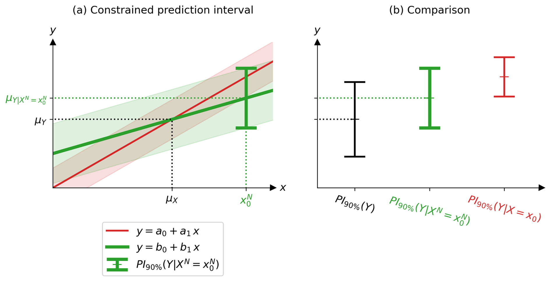
Figure 8 (a) Example showing, in green and bold, the 90 % probability interval (PI) of the projected variable Y constrained by the noisy observation $x_{\mathrm{0}}^N$, as described by Eq. (24). The green colour (bold line) corresponds to the case where the observation is noisy, while the red colour (non-bold line) corresponds to the case where the observation is considered noiseless, as in the previous section. (b) Comparison between the 90 % PI of Y unconstrained (black, on the left), constrained by a noisy observation (green, in the middle), and constrained by a noiseless observation (red, on the right) corresponding, respectively, to Eq. (2), Eq. (24), and Eq. (14). The values of the means, variances, etc. are given in Appendix D.

The expression of the PI of Y constrained by a noisy observation ($\mathrm{PI}\left(Y\right|X^N=x_{\mathrm{0}}^N)$) has a form close to that in which the observational noise was neglected, as in the previous section ($\mathrm{PI}\left(Y\right|X=x_{\mathrm{0}})$). As before, the expectation of Y constrained is directly the real-world observation fed into the regression (see Eq. 20), and the variance of Y constrained is the variance of the regression error (see Eq. 22). The constraint corrects the expectation (see Eq. 21) and reduces the variance (see Eq. 23). However, the difference between including or not including the observational noise (difference between green and red in Fig. 8) lies in a term called here the attenuation coefficient: $\mathrm{1}/(\mathrm{1}+\mathrm{1}/{\mathrm{SNR}}^{\mathrm{2}})$. The slope considering the observational noise, b₁, is attenuated compared to the slope neglecting the observational noise, a₁: $b_{\mathrm{1}}=a_{\mathrm{1}}/(\mathrm{1}+\mathrm{1}/{\mathrm{SNR}}^{\mathrm{2}})$. The larger the observational noise, the greater the attenuation. This is illustrated in Fig. 8a, where the linear relationship is stronger when the observational noise is neglected (red) than when it is included (green). In this example, there is as much signal as noise (SNR=1). The attenuation coefficient is therefore 50 %. In reality, depending on the application, the observational noise can be very small, although it is difficult to estimate, especially for low-frequency internal variability, which can lead to serious overconfidence (Bonnet et al., 2021). This attenuation coefficient, $\mathrm{1}/(\mathrm{1}+\mathrm{1}/{\mathrm{SNR}}^{\mathrm{2}})$, weakens both the expectation correction and the variance reduction, as described in Eqs. (21) and (23), respectively. This highlights the need to account for observational noise; otherwise the PI of Y constrained will be overconfident, with too strong an expectation correction.

The use of the PI of $Y|X^N=x_{\mathrm{0}}^N$ described by Eq. (24) requires knowledge of the parameters b₀, b₁, and ${\mathit{\sigma }}_{{\mathit{\epsilon }}^N}$, which are unknown in reality. As in the previous section, an ensemble of M climate model projections is used to estimate them. The estimators of a₀, a₁, and ${\mathit{\sigma }}_{{\mathit{\epsilon }}^N}$ are given in Table A2. Using them, it is shown in Appendix H that the confidence interval (CI) of Y constrained by a noisy observation is:

$$\begin{array}{}\text{(25)}& \begin{array}{rl}{\mathrm{CI}}_{\mathrm{1}-\mathit{\alpha }}& \left(Y|X^N=x_{\mathrm{0}}^N\right)=\left[{\widehat{b}}_{\mathrm{0}}+{\widehat{b}}_{\mathrm{1}}{x}_{\mathrm{0}}^N\pm t^{M-\mathrm{2}}{\widehat{\mathit{\sigma }}}_{{\mathit{\epsilon }}^N}\right.\\ & \left.\sqrt{\mathrm{1}+{\displaystyle \frac{\mathrm{1}}{M}}+{\displaystyle \frac{{\left(x_{\mathrm{0}}^N-{\widehat{\mathit{\mu }}}_X\right)}^{\mathrm{2}}}{M\left({\widehat{\mathit{\sigma }}}_X^{\mathrm{2}}+{\mathit{\sigma }}_N^{\mathrm{2}}\right)}}}\right].\end{array}\end{array}$$

When X is multivariate, its expression is:

$$\begin{array}{}\text{(26)}& \begin{array}{rl}{\mathrm{CI}}_{\mathrm{1}-\mathit{\alpha }}& \left(Y|{\mathbf{X}}^N={\mathbf{x}}_{\mathrm{0}}^N\right)=\left[{\widehat{b}}_{\mathrm{0}}+{\widehat{\mathbf{b}}}_{\mathrm{1}}^T{\mathbf{x}}_{\mathrm{0}}\pm t^{M-\mathrm{1}-p}{\widehat{\mathit{\sigma }}}_{{\mathit{\epsilon }}^N}\right.\\ & \left.\sqrt{\mathrm{1}+{\displaystyle \frac{\mathrm{1}}{M}}+{\left({\mathbf{x}}_{\mathrm{0}}-{\widehat{\mathit{\mu }}}_X\right)}^T{\displaystyle \frac{{\left({\widehat{\mathbf{\Sigma }}}_X+{\mathbf{\Sigma }}_N\right)}^{-\mathrm{1}}}{M}}\left({\mathbf{x}}_{\mathrm{0}}-{\widehat{\mathit{\mu }}}_X\right)}\right],\end{array}\end{array}$$

where p is the number of features in X and Σ_X and Σ_N are the variance-covariance matrices of X and N, respectively. The confidence interval of Y constrained by a noisy observation (${\mathrm{CI}}_{\mathrm{1}-\mathit{\alpha }}\left(Y\right|X^N=x_{\mathrm{0}}^N)$) described in Eq. (26) is the statistical model called “CLimate variable confidence Interval of Multivariate Linear Observational COnstraint” (ClimLoco1.0). To illustrate these mathematical results, Fig. 9 shows two realisations of ClimLoco1.0: one realisation from the sample (X₁, Y₁), …, (X_M, Y_M) of size M=5 and one realisation from the sample of size M=30, taken from the same synthetic example as before. In Fig. 9a, each sample realisation gives a different realisation of the linear relationship $y={\widehat{b}}_{\mathrm{0}}+{\widehat{b}}_{\mathrm{1}}x$ (green line) and a realisation of the confidence interval constrained by a noisy observation described in Eq. (25) (green interval). The green shading represents the ${\mathrm{CI}}_{\mathrm{90}\mathit{\%}}\left(Y\right|X^N=x_{\mathrm{0}}^N)$ obtained for different positions of the observation $x_{\mathrm{0}}^N$. For comparison, this Fig. 9a shows in red the ${\mathrm{CI}}_{\mathrm{90}\mathit{\%}}\left(Y\right|X=x_{\mathrm{0}})$ for different positions of x₀ (red shading). This enables us to compare the difference in the width and centre of the intervals, whether the observational noise is considered or neglected. Fig. 9b compares the CI of Y: unconstrained (CI_90 %(Y), in black), constrained by a noiseless observation (${\mathrm{CI}}_{\mathrm{90}\mathit{\%}}\left(Y\right|X=x_{\mathrm{0}})$, in red), and constrained by a noisy observation (ClimLoco1.0, ${\mathrm{CI}}_{\mathrm{90}\mathit{\%}}\left(Y\right|X^N=x_{\mathrm{0}}^N)$, in green).

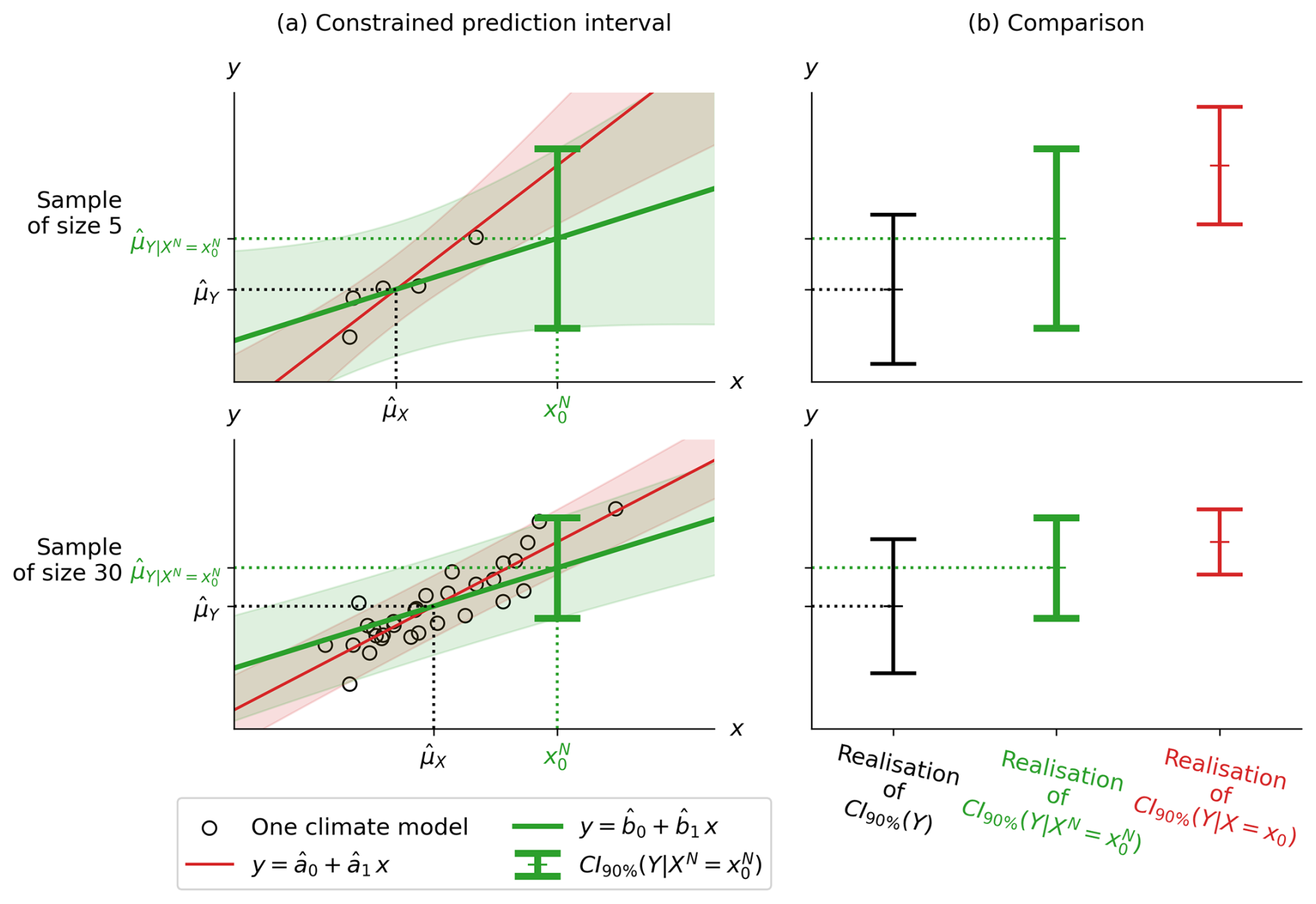
Figure 9 Synthetic example showing (a) the first column with two realisations of the confidence interval (CI) of Y constrained by noisy and noiseless observations, shown in green (bold) and red (non-bold), respectively, at a 90 % confidence level. The shadings correspond to the intervals obtained from different positions of the observation. The first and second rows correspond to a realisation of a sample of size M=5 and M=30, respectively. (b) The second column compares the CIs of Y unconstrained (black, on the left), constrained by a noiseless observation (red, on the right), and constrained by a noisy observation (green, in the middle) corresponding, respectively, to Eq. (6),  Eq. (25), and  Eq. (15). The details of the data simulation are given in Appendix D.

When comparing the CI of Y constrained by a noisy vs. noiseless observation (green vs. red in Fig. 9b), the same conclusions are reached as when comparing PI of Y constrained by noisy vs. noiseless observation; there is a decrease in the reduction of uncertainty (interval width) and in the correction of the best guess (interval centre). In other words, observational noise weakens the constraint. When comparing the two rows of Fig. 9, corresponding to a small (first row) and a large sample (second row), the large sample leads to narrower CI. The CI is more precise when estimated from more data. This is visible in all three expressions of the CI discussed in this article through the effect of the term M. Moreover, this synthetic example uses strong observational noise (SNR=1). Combined with a small sample (first row of Fig. 9) this tends to make the $\mathrm{CI}\left(Y\right|X^N=x_{\mathrm{0}}^N)$ large, meaning that the uncertainty is large. Therefore, the $\mathrm{CI}\left(Y\right|X^N=x_{\mathrm{0}}^N)$ is larger than the CI(Y) in the second row: the constraint has not reduced the uncertainty, which is surprising. However, this is an extreme case, combining both high observational noise and small sample size. In summary, low observational noise combined with a high correlation between X and Y leads to a strong constraint, which means a strong best guess correction (centre of the confidence interval) and a strong uncertainty reduction (width of the confidence interval). Uncertainty is also affected by the sample size: the larger the sample size, the greater the uncertainty reduction. The best guess correction is also affected by the distance between the observation and the multi-model mean ($x_{\mathrm{0}}-{\widehat{\mathit{\mu }}}_X$), which is called in this article the “multi-model bias”. The larger the bias, the greater the correction.

The main contributions of this section are to provide the statistical model ClimLoco1.0, the confidence interval of the projected variable constrained by a noisy observation, to express and illustrate it graphically as an attenuated linear regression, and to highlight the need to take this observational noise into account and to have a sample size as large as possible. Figure 10 is proposed as an illustrative summary of a comparing the CI of Y unconstrained, of Y constrained by a noiseless observation, and of Y constrained by a noisy observation. This figure is built using synthetic data detailed in Appendix D.

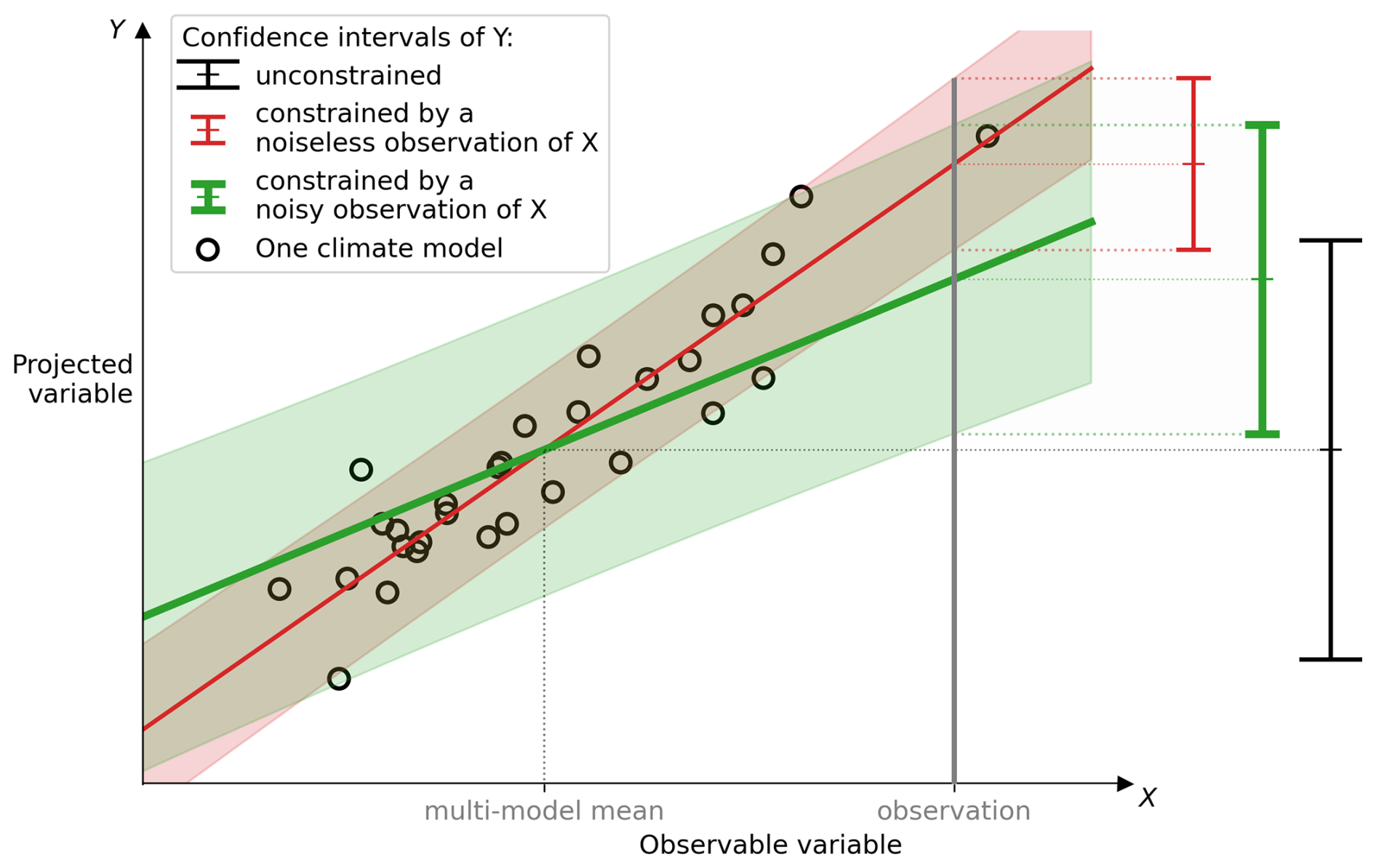
Figure 10 Graphical representation of the effect of considering observational noise in a linear observational constraint (OC). (i) In red (non-bold), the observational noise is neglected. (ii) In green (bold), the observational noise is considered, which is more rigorous. The latter confidence interval (CI) corresponds to the statistical model ClimLoco1.0, presented in this article. (i) When observational noise is neglected, a linear relationship is defined between a past observable variable X and a future variable Y using an ensemble of climate models (black circles). The slope and error of the relationship between X and Y are shown as the red line and shading, respectively. A real-world observation of X is then fed into the linear relationship to obtain the CI of Y constrained (red interval, non-bold). Compared with the CI of Y unconstrained (black interval, with the large tails), the CI of Y constrained (red interval, non-bold) has a reduced uncertainty (interval width) and a corrected best guess (interval centre). The intensity of the best guess correction (between unconstrained and constrained) depends on the slope between X and Y and the difference between the multi-model mean and the observation (the “multi-model bias”). (ii) However, it does not take into account the uncertainty associated with the real-world observation. When taken into account, observational noise reduces the slope (green line, in bold) of the linear relationship and increases its error (green shading). Consequently, the CI of Y constrained by a noisy observation (green interval, bold) has less uncertainty reduction and a smaller best guess correction than the CI of Y constrained by a noiseless observation (red interval, non-bold). All three CIs use a 90 % confidence level.

5 Comparison with the literature

In this section, the results of this article are compared with those of some of the most widely used approaches in the observational constraint literature: (a) Ribes et al. (2021) and Bowman et al. (2018) and (b) Cox et al. (2018).

• a.

  Both Ribes et al. (2021) and Bowman et al. (2018) use statistical approaches to constrain Y by real-world observations. One can demonstrate (not shown here) that these two articles yield equivalent expressions for the expectation and variance of $Y|X^N=x_{\mathrm{0}}^N$. The main difference between them is that the first article considers the variables X and Y as univariate and the second as multivariate, respectively. It can be seen that these articles have the same expressions for the expectation and variance of $Y|X^N=x_{\mathrm{0}}^N$ as those obtained in Eqs. (21) and (23). This means that the approaches of both Ribes et al. (2021) and Bowman et al. (2018) are equivalent to using a linear regression model (multivariate and univariate, respectively). As seen in the previous section, this regression is corrected for the observational noise. This is an important result for interpreting these methods using linear regression, as is done in our article. Furthermore, an important caveat to this equivalence is that there is a well-known risk of overfitting when using multivariate linear regression, i.e. learning incorrect relationships between features by over-fitting the data. This risk is greater when the number of variables is large and the number of climate models used to learn the regression is small. The multivariate method developed by Ribes et al. (2021) therefore presents a risk of overlearning.

  Furthermore, the articles by Bowman et al. (2018) and Ribes et al. (2021) only gave the theoretical expressions for the expectation and variance of $Y|X^N=x_{\mathrm{0}}^N$. These theoretical values are in reality unknown. They did not provide details of the exact expression of the estimates, which – as previously seen using confidence intervals – leads to a higher uncertainty due to the limited sample size. This can be neglected when the sample size is very large, but it becomes very important when the sample size is small, as shown in the previous section (see Eq. 6). In climate science, sample sizes are usually small (especially when considering high-resolution models; Bauer et al., 2021), so that we argue here that this uncertainty must be included in the estimates.

• b.

  When referring to observational constraints, an often quoted figure comes from Eyring et al. (2019), Box 1. This method is used in several papers, e.g. Bracegirdle and Stephenson (2012), Brient (2020). This figure is interpreted here using the well-known paper by Cox et al. (2018). Our approach leads to a different expression for the expectation and variance of Y constrained by a noisy observation than the approach of Cox et al. (2018), for which we argue our disagreement here. Cox et al. (2018) studies the distribution of Y using the law of total probability (see Eq. 15 in Cox et al., 2018). Written differently, using the laws of total expectation and variance, the expectation and variance of this distribution can be expressed as:

  $$\begin{array}{}\text{(27)}& {\displaystyle }& {\displaystyle }\mathbb{E}\left[Y\right]=\mathbb{E}\left[\mathbb{E}\right[Y\left|X\right]],\text{(28)}& {\displaystyle }& {\displaystyle }\mathbb{V}\left(Y\right)=\mathbb{E}\left[\mathbb{V}\right[Y\left|X\right]]+\mathbb{V}[\mathbb{E}\left[Y\right|X\left]\right].\end{array}$$

  Using a linear regression between Y and X, noted $Y=a_{\mathrm{0}}+a_{\mathrm{1}}X+\mathit{\epsilon }$, it gives:

  $$\begin{array}{}\text{(29)}& {\displaystyle }& {\displaystyle }\mathbb{E}\left[Y\right]=a_{\mathrm{0}}+a_{\mathrm{1}}\mathbb{E}\left[X\right],\text{(30)}& {\displaystyle }& {\displaystyle }\mathbb{V}\left(Y\right)=\mathbb{V}\left(\mathit{\epsilon }\right)+a_{\mathrm{1}}^{\mathrm{2}}\mathbb{V}\left(X\right).\end{array}$$

  Cox et al. (2018) assumes that X follows a distribution centred around the observation ($\mathbb{E}\left[X\right]=x_{\mathrm{0}}^N$) and with a variance equal to the observational noise variance ($\mathbb{V}\left(X\right)={\mathit{\sigma }}_N^{\mathrm{2}}$). Consequently,

  $$\begin{array}{}\text{(31)}& {\displaystyle }& {\displaystyle }\mathbb{E}\left[Y\right]=a_{\mathrm{0}}+a_{\mathrm{1}}{x}_{\mathrm{0}}^N,\text{(32)}& {\displaystyle }& {\displaystyle }\mathbb{V}\left(Y\right)=\mathbb{V}\left(\mathit{\epsilon }\right)+a_{\mathrm{1}}^{\mathrm{2}}{\mathit{\sigma }}_N^{\mathrm{2}}.\end{array}$$

  This corresponds to the figure in Eyring et al. (2019), Box 1: the best guess is directly the observation fed into the regression (a₀+a₁x₀), and the total uncertainty is the sum of regression uncertainty (𝕍(ε)) and the observational uncertainty propagated through the regression ($a_{\mathrm{1}}^{\mathrm{2}}{\mathit{\sigma }}_N^{\mathrm{2}}$).

We suggest that there are two main problems with this approach. Firstly, Cox et al. (2018) use two different distributions of the same variable X: one from the climate models to learn the linear relationship $Y=a_{\mathrm{0}}+a_{\mathrm{1}}X+\mathit{\epsilon }$ and one from the noisy observation. However, the climate models have a different X distribution from the observation: $\mathbb{E}\left[X\right]={\mathit{\mu }}_X\ne x_{\mathrm{0}}^N$ and $\mathbb{V}\left(X\right)={\mathit{\sigma }}_X^{\mathrm{2}}\ne {\mathit{\sigma }}_N^{\mathrm{2}}$. The variable X cannot have two different expectations or two different variances; therefore, Eqs. (31) and (32) written above are incorrect from our point of view. It is necessary to distinguish the variable X, whose distribution is given by the climate models, and the variable X^N, which is observed from the real world with observational noise, as is done in this article. Secondly, the constrained variable should be denoted $Y|X^N=x_{\mathrm{0}}^N$, not just Y. This has a major effect on the resulting equations. Indeed, Eqs. (29) and (30) are correct, but they do not constrain either the expectation or the variance of Y.

This conclusion is consistent with Hall et al. (2019), who states that “care must be taken to characterise the uncertainty in the observational values of the X variable. The translation of observed X-values into predicted Y-values is not trivial. It is certainly not as simple as finding the intersection of the most likely value of observed X and the regression line relating Y to X and `reading' the predicted Y value. Instead, both observed X and predicted Y must be treated statistically”. The clarification proposed here may help to move in this direction.

A key feature of this article is the use of multiple observable variables simultaneously (i.e. a multivariate approach). Most approaches in the literature are univariate. However, we identified some multivariate approaches. As mentioned in this section, Ribes et al. (2021) use a linear multivariate approach. The other approaches in the literature are mainly non-linear, making use of the large amount of information provided by multiple variables in more complex regression models. However, due to the non-linearity, it is not possible to formulate an analytical expression for the confidence interval. For instance, Schlund et al. (2020) constrain future gross primary production (GPP) using a regression model based on random forest (gradient-boosted regression trees) that takes into account past GPP, temperature, precipitation, etc. To estimate uncertainty, the non-linear model is locally approximated by a linear one.

6 Discussion of the assumptions

The different assumptions used to obtain ClimLoco1.0 are all compiled in the following list. Climate models are supposed to be (i) random and independent realisations of the same (ii) Gaussian distributions as (iii) reality. (iv) The observations are noisy realisations of reality, with additive Gaussian noise that is independent of X. Its covariance is assumed to be known. Each assumption is detailed below. If possible, we evaluate its impact on the results and provide insights into how it could be addressed in the next version of ClimLoco1.0.

• i.

  ClimLoco1.0 assumes that climate models are independent and equally plausible. This assumption is used by most OC methods, except those that assign weights to climate models (e.g. Brunner et al., 2019). However, defining confidence intervals using weighted samples without these assumptions is challenging, and this is an area in which ClimLoco1.0 could be improved. In ClimLoco1.0, these assumptions virtually give too much importance to dependent climate models, as if there were duplicates in the data. Groups of dependent climate models are closer together in the (X, Y) space, as observed for climate models belonging to the same institute, for example. Groups of models that are close together pull the best guess towards them and reduce the inter-model spread, leading an underestimation of the uncertainty.

• ii.

  The assumption that the distributions are Gaussian is clearly recognised as potentially questionable, e.g. in regard to precipitation. If the distribution is not centred, the confidence interval should not be centred either. If the distribution has significant tails, the limits of the confidence interval must be further apart. The greater the difference between the distribution and a Gaussian distribution, the less accurate ClimLoco1.0 will be in estimating the limits of the confidence interval. However, we did not estimate here whether this impact is significant or negligible. To address this issue in future developments of ClimLoco1.0 using non-Gaussian distributions, we recommend employing a bootstrap method to empirically derive a confidence interval. Bootstrapping involves repeatedly resampling the dataset with replacement to create different sub-datasets. Each sub-dataset yields a different observational constraint result. These distributions are then used to compute a confidence interval. However, in this case, no analytical expression of the confidence interval can be derived, as this remains an empirical approach.

• iii.

  It is necessary to assume that climate models have the same distributions as reality; otherwise, they cannot be used to predict the future. However, as mentioned in Sanderson et al. (2021), the relationship between x and y emerging from climate models may be due to shared errors and may not actually exist. Therefore, multiple lines of evidence must be used to validate this relationship before it can be applied. Employing an incorrect relationship will lead to an incorrect confidence interval.

• iv.

  It also seems reasonable to assume that the observational noise has a centred distribution, as the instrument error and internal variability are expected to be centred. In many cases, the Gaussianity of the distribution of the observations may also be a reasonable assumption. This is demonstrated in our case study using HadCRUT 5 (see Sect. I). Assuming that the observational noise is independent of the climate model distribution is also reasonable, since the instrumental error and real-world internal variability are not related to climate models. However, by assuming that the covariance of the observational noise is known, we neglect the uncertainty arising from its estimation. In our case study, we use HadCRUT 5 to estimate the covariance matrix of the observational noise. As it provides 200 ensemble members, the estimation error of the covariance matrix should be very low. Finally, internal variability is considered only for the observations in ClimLoco1.0, even though it is also present in climate models. Depending on the climate variable used, this could slightly increase the uncertainty. One promising approach is to consider the distribution of values from each climate model, as outlined in Olson et al. (2018).

7 Conclusions

A confidence interval for future climate, i.e. a best guess of the future climate with uncertainty given at a confidence level, can be obtained from an ensemble of climate model projections. However, the large dispersion between climate model projections makes this interval large, and consequently the future climate very uncertain. To refine it, methods called observational constraints (OCs) combine climate model projections with some real-world observations (cf. Lee et al. (2021)). These methods are now increasingly used (O'Reilly et al., 2024), even by potential stakeholders at the national level (e.g. Ribes et al., 2022). They therefore deserve to be rigorously described in their assumptions and mathematical description. However, there are many challenges in dealing with the literature of OC. There is a wide variety of OC methods, which are sometimes difficult to reproduce and may lack mathematical detail, which are usually limited to the use of a single observable variable to constrain, and which do not strictly use confidence intervals, which are essential to correctly define uncertainty.

To address these challenges, this article proposes a new (1.0) statistical method, ClimLoco, which stands for “CLimate variable confidence Interval of Multivariate Linear Observational COnstraint”. ClimLoco1.0 describes the confidence interval of a projected variable constrained by a noisy observation using a linear multivariate framework. It is inspired by the theory of measurement error models from Fuller (2009). We found that constraining a projected variable has two effects: it corrects the best guess of the projected variable according to the multi-model bias (the difference between the multi-model mean and the real-world observation) and reduces the associated uncertainty.

Compared with the existing literature, ClimLoco1.0 provides a more rigorous expression of uncertainty through the use of confidence intervals. This takes into account the quality of the estimators of the best guess and the uncertainty of a projected variable, which depends in particular on the number of climate models used. We have therefore emphasised the need to have as large an ensemble of models as possible, in order to obtain the most accurate estimates. In addition, ClimLoco1.0 takes into account the observational noise in a rigorous framework, which is important to correctly estimate the uncertainty. We find a new graphical interpretation (cf. Fig. 10), of the effect of observational noise, which weakens the constraint (less reduction of uncertainty and a smaller change in the best guess). This article is intended to be didactic, building the statistical model ClimLoco1.0 step by step, from the unconstrained case to the case constrained by noisy observations, and illustrating each step with univariate examples.

In addition, the results are compared with some of the most commonly used methods in the literature: “statistical” methods (e.g. Bowman et al., 2018; Ribes et al., 2021) and “linear regression” methods (e.g. Cox et al., 2018). There are strong similarities between the statistical methods of Bowman et al. (2018) and Ribes et al. (2021) and the multivariate linear regression OC developed in this article. We argue that there is an equivalence between their methods and a multiple linear regression. This implies that the methods are subject to the risk of overfitting (i.e. learning incorrect relationships between features by over-fitting the data). The use of methods to limit overfitting, such as ridge regression, seems to be a promising perspective in this respect. However, since Bowman et al. (2018) and Ribes et al. (2021) did not use confidence intervals, they neglect the quality of the estimators, which depends on the number of climate models considered. They therefore underestimate the uncertainty. There is a major discrepancy between our method and that of Cox et al. (2018), which is now widely used for linear regression OCs. We highlight problems in the underlying mathematics and propose a new figure (Fig. 10), which may be more appropriate than Fig. 1 from Eyring et al. (2019), to describe exactly how linear OC works in a geometric sense.

The statistical model ClimLoco1.0 is an effort to better account for uncertainties and bring more clarity to OC methods. However, there are still some challenges to overcome, for example, considering non-Gaussian distributions, dependence between climate models, non-linear regression, etc. These are interesting perspectives to build more advanced versions of ClimLoco1.0. Finally, finding equivalences between OC methods, as performed here, can be very useful to bring more clarity to the large literature of OC methods. For example, Karpechko et al. (2013) succeeded in converting a linear regression into climate model weights, but neglected the observational noise.

As an extension of this article, Appendix I illustrates the use of ClimLoco1.0 in a real case study and performs some sensitivity tests. The Python code and data, along with a simple, user-friendly example to replicate ClimLoco1.0, are provided via the “Code and data availability” section.

Appendix A: Summary

Table A1 Confidence intervals (CI) of Y unconstrained, constrained by a noiseless observation, and constrained by a noisy observation. Within each case, the results when X is univariate (X∈IR) and when X is multivariate (X∈IR^p) are both given. Since the first case does not depend on X, it is the same whether X is univariate or multivariate. The different estimators are listed in Table A2 and described in the main part of the article.

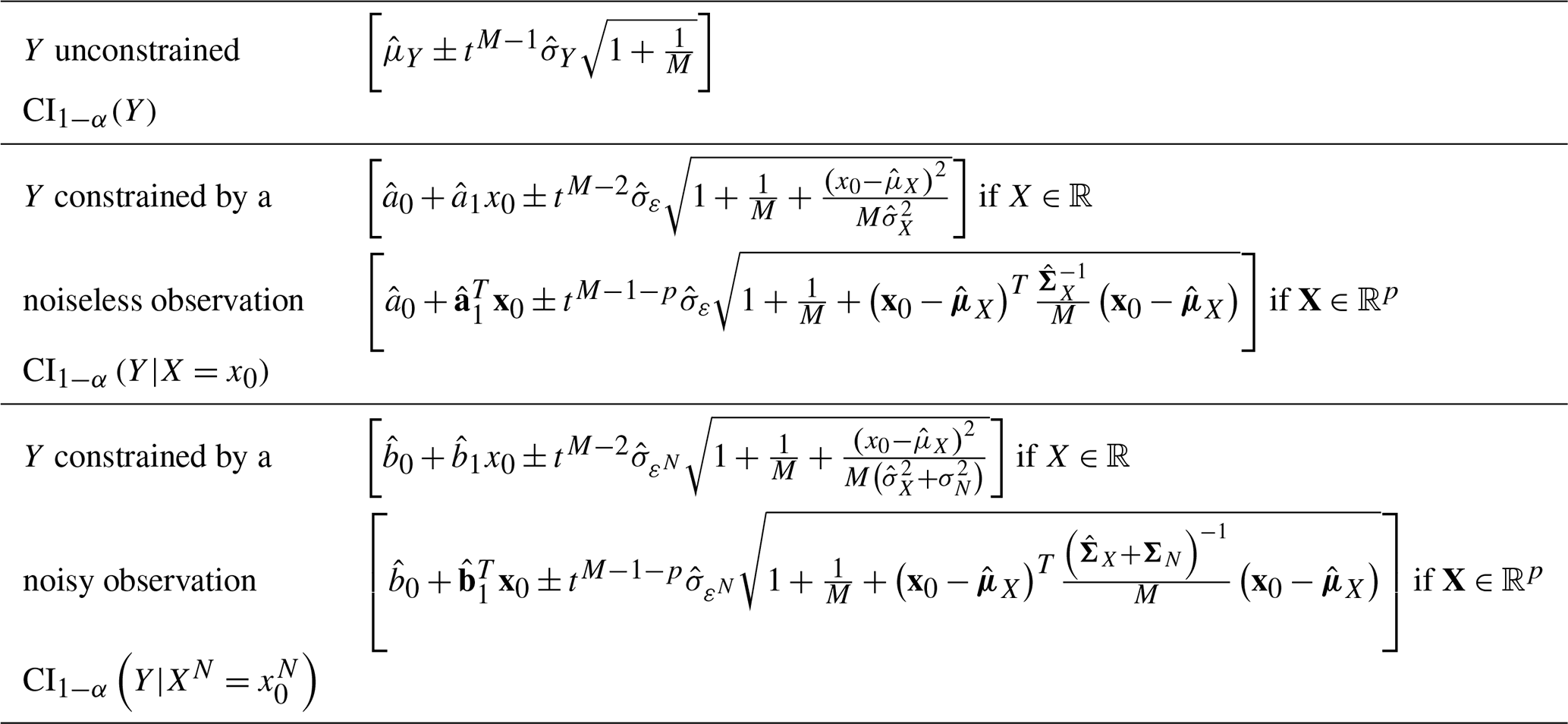
Table A2 Definition of the estimators used in this article, when X is univariate (X∈IR) and when X is multivariate (X∈IR^p).

Appendix B: Key statistical concepts

This section outlines the key statistical concepts required to grasp the construction of ClimLoco1.0. The demonstrations and formulas can be found in the article.

Y is a variable representing, for example, the global mean surface air temperature (GSAT) in 2100. Its actual value is unknown, but we assume that its distribution – also known as a probability density function (PDF) – is known. For example, Y can follow a Gaussian PDF, as illustrated in Fig. B1a. Y is called a random variable because it takes random values that follow the probability given by its PDF. These random values are called realisations of Y. This PDF can be used to compute a probability interval, i.e. an interval containing the actual value of Y with a given probability. The 90 % probability interval of Y is shown in Fig. B1a, where a probability level of 90 % corresponds to 90% of the area under the PDF (shown in grey). In this example, the GSAT anomaly in 2100 lies within the interval [2.9, 4.1 °C] with a probability of 90 %. The probability level, denoted 1−α in our article, is a user-selectable parameter. A higher probability level would give a wider interval as there is a greater chance that it will contain the actual value. It is common to use a probability level of 68 %, as this corresponds to ± 1 standard deviation for a Gaussian PDF.

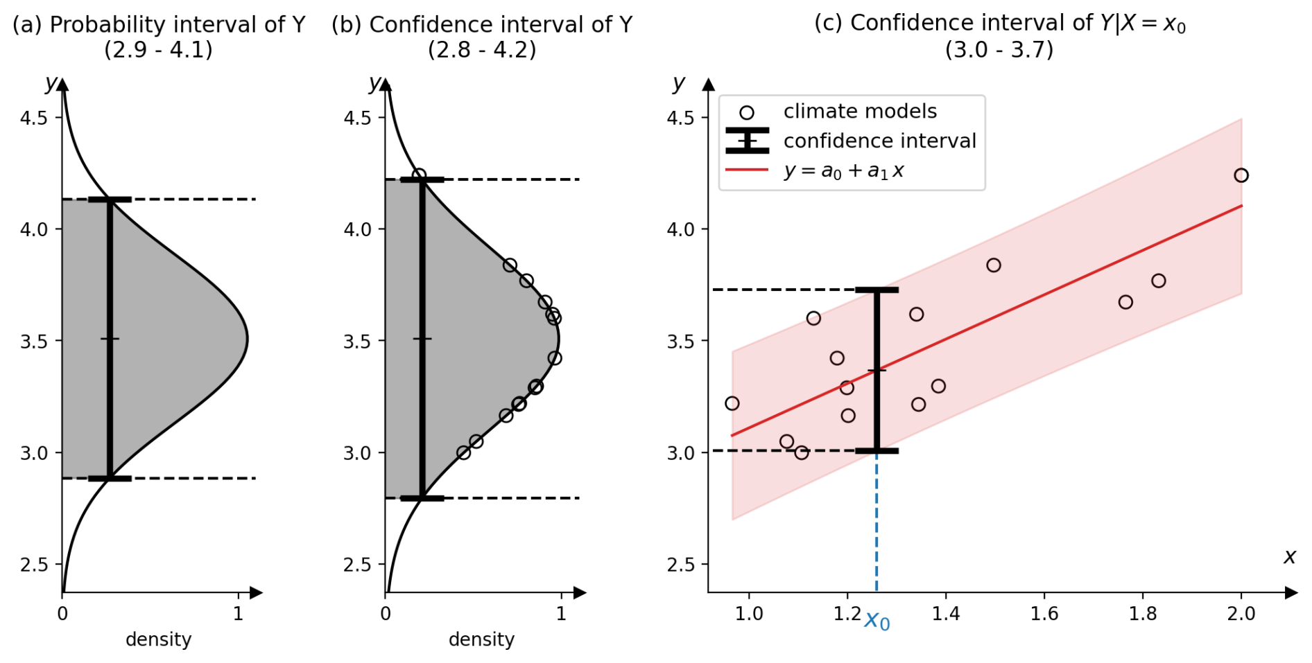
Figure B1 Example of a 90 % probability and confidence interval of Y (a, b) and a confidence interval of $Y|X=x_{\mathrm{0}}$ (c). Y is the global mean surface air temperature (GSAT), averaged over the period 2081–2100 and expressed in degrees Celsius (°C). X is the GSAT average in 2015–2024, also in °C. Here, 15 climate models are considered. For more information, see Sect. I.

However, in a real case, the parameters of the PDF of Y are unknown. In climate science, we use climate models to estimate these parameters. Each climate model simulates Y, producing a variable called Y_i. Running a climate model produces a realisation, denoted by y_i. Assuming that each Y_i follows the same PDF as Y, the M climate models yield a sample of M random variables, denoted by (Y₁,, …, Y_M). The realisation of this sample is denoted as (y₁, …, y_M). The expectation and standard deviation can be estimated using this sample to estimate the PDF. However, the estimators of the expectation and standard deviation introduce errors due to the limited sample size (M). Therefore, we cannot simply take the probability interval of this estimated PDF, as is often seen in the literature. When these errors are considered, the resulting interval is wider and is associated with a Student's t-distribution with M−1 degrees of freedom. The number of degrees of freedom of a Student's t-distribution controls its shape, making it closer to a Gaussian PDF when it is small and with a higher spread when it is large. As different realisations of the sample give different intervals, the term “confidence interval” is used instead of “probability interval”. A confidence interval is sometimes also called a prediction interval. Using the previous example of the 2100 anomaly of GSAT, the 90 % confidence interval is [2.8, 4.2 °C], as illustrated in Fig. B1b.

To obtain a refined interval, we can use the PDF of Y given the observation x₀ of a random variable X, denoted $Y|X=x_{\mathrm{0}}$. As before, the parameters of the PDF of $Y|X=x_{\mathrm{0}}$ are unknown but can be estimated using a sample of climate models. As demonstrated in this article, this can be represented by a linear relationship between X and Y: $Y=a_{\mathrm{0}}+a_{\mathrm{1}}X+\mathit{\epsilon }$, where a₀ is the intercept, a₁ is the slope, and ε is the regression error. The confidence interval and the linear relationship are illustrated in Fig. B1c, using the same example as before. In this example, the 90 % confidence interval of $Y|X=x_{\mathrm{0}}$ is [3.0, 3.7 °C]. This is smaller than the confidence interval of Y, owing to the additional information provided by the observation x₀. Finally, when X is multivariate, this is equivalent to multivariate linear regression: $Y=a_{\mathrm{0}}+{\mathbf{a}}_{\mathrm{1}}^T\mathbf{X}+\mathit{\epsilon }$, where a₁ is a p-dimensional vector and X is a matrix with p columns (and M rows), with p denoting the number of variables.

Appendix C: Confidence interval of Y

The goal of this appendix is to find the confidence interval of Y. For this purpose, it is assumed that Y follows a Gaussian distribution: $Y\sim \mathcal{N}({\mathit{\mu }}_Y,{\mathit{\sigma }}_Y^{\mathrm{2}})$. To estimate μ_Y and ${\mathit{\sigma }}_Y^{\mathrm{2}}$, it uses a sample of M random variables, denoted by (Y₁, …, Y_M), given by an ensemble of M climate models. These random variables are assumed to be independent and to follow the same law as Y. The classical estimators of the expectation and variance are:

$$\begin{array}{ll}{\displaystyle }& {\displaystyle }{\widehat{\mathit{\mu }}}_Y={\displaystyle \frac{\mathrm{1}}{M}}\sum _{i=\mathrm{1}}^M{Y}_i\mathrm{and}{\widehat{\mathit{\sigma }}}_Y^{\mathrm{2}}={\displaystyle \frac{\mathrm{1}}{M-\mathrm{1}}}\sum _{i=\mathrm{1}}^M{\left(Y_i-{\widehat{\mathit{\mu }}}_Y\right)}^{\mathrm{2}}.\\ {\displaystyle }& {\displaystyle }\mathrm{On}\mathrm{the}\mathrm{one}\mathrm{hand},E\left[{\widehat{\mathit{\mu }}}_Y\right]={\displaystyle \frac{\mathrm{1}}{M}}\sum _{i=\mathrm{1}}^{M}E\left[Y_i\right]={\displaystyle \frac{\mathrm{1}}{M}}\sum _{i=\mathrm{1}}^M{\mathit{\mu }}_Y={\mathit{\mu }}_Y\\ {\displaystyle }& {\displaystyle }\mathrm{and}\mathrm{Var}\left({\widehat{\mathit{\mu }}}_Y\right)={\displaystyle \frac{\mathrm{1}}{M^{\mathrm{2}}}}\sum _{i=\mathrm{1}}^M\mathrm{Var}\left(Y_i\right)={\displaystyle \frac{\mathrm{1}}{M^{\mathrm{2}}}}\sum _{i=\mathrm{1}}^M{\mathit{\sigma }}_Y^{\mathrm{2}}={\displaystyle \frac{{\mathit{\sigma }}_Y^{\mathrm{2}}}{M}}\\ {\displaystyle }& {\displaystyle }\Rightarrow {\widehat{\mathit{\mu }}}_Y\sim \mathcal{N}\left({\mathit{\mu }}_Y,{\displaystyle \frac{{\mathit{\sigma }}_Y^{\mathrm{2}}}{M}}\right)\end{array}$$

$$\begin{array}{ll}{\displaystyle }& {\displaystyle }\Rightarrow Y-{\widehat{\mathit{\mu }}}_Y\sim \mathcal{N}\left(\mathrm{0},{\mathit{\sigma }}_Y^{\mathrm{2}}\left(\mathrm{1}+{\displaystyle \frac{\mathrm{1}}{M}}\right)\right)\\ {\displaystyle }& {\displaystyle }\Rightarrow {\displaystyle \frac{Y-{\widehat{\mathit{\mu }}}_Y}{{\mathit{\sigma }}_Y\sqrt{\mathrm{1}+\frac{\mathrm{1}}{M}}}}\sim \mathcal{N}(\mathrm{0},\mathrm{1})\\ {\displaystyle }& {\displaystyle }\mathrm{On}\mathrm{the}\mathrm{other}\mathrm{hand},{\widehat{\mathit{\sigma }}}_Y^{\mathrm{2}}={\displaystyle \frac{\mathrm{1}}{M-\mathrm{1}}}\sum _{i=\mathrm{1}}^M{\left(Y_i-{\widehat{\mathit{\mu }}}_Y\right)}^{\mathrm{2}}\\ {\displaystyle }& {\displaystyle }\Rightarrow (M-\mathrm{1}){\displaystyle \frac{{\widehat{\mathit{\sigma }}}_Y^{\mathrm{2}}}{{\mathit{\sigma }}_Y^{\mathrm{2}}}}=\sum _{i=\mathrm{1}}^M{\displaystyle \frac{{\left(Y_i-{\widehat{\mathit{\mu }}}_Y\right)}^{\mathrm{2}}}{{\mathit{\sigma }}_Y^{\mathrm{2}}}}\\ {\displaystyle }& {\displaystyle }\mathrm{As}{\displaystyle \frac{\left(Y_i-{\widehat{\mathit{\mu }}}_Y\right)}{{\mathit{\sigma }}_Y}}\sim \mathcal{N}(\mathrm{0},\mathrm{1})\\ {\displaystyle }& {\displaystyle }\mathrm{then}(M-\mathrm{1}){\displaystyle \frac{{\widehat{\mathit{\sigma }}}_Y^{\mathrm{2}}}{{\mathit{\sigma }}_Y^{\mathrm{2}}}}\sim {\mathit{\chi }}^{\mathrm{2}}(M-\mathrm{1})\end{array}$$

Or

$$\left\{\begin{array}{l}U\sim \mathcal{N}(\mathrm{0},\mathrm{1})\\ V\sim {\mathit{\chi }}^{\mathrm{2}}\left(n\right)\\ U⟂⟂V\end{array}\right.\Rightarrow {\displaystyle \frac{U}{\sqrt{V/n}}}\sim \mathrm{St}\left(n\right),$$

with $⟂⟂$ as the sign of independence and St(n) as the student distribution with n degrees of freedom. Consequently, by noting $U=\frac{Y-{\widehat{\mathit{\mu }}}_Y}{{\mathit{\sigma }}_{\mathit{\epsilon }}\sqrt{\mathrm{1}+\frac{\mathrm{1}}{M}}}$ and $V=(M-\mathrm{1})\frac{{\widehat{\mathit{\sigma }}}_Y^{\mathrm{2}}}{{\mathit{\sigma }}_Y^{\mathrm{2}}}$, this implies that: $\frac{U}{\sqrt{V/(M-\mathrm{1})}}=\frac{Y-{\widehat{\mathit{\mu }}}_Y}{{\widehat{\mathit{\sigma }}}_Y\sqrt{\mathrm{1}+\frac{\mathrm{1}}{M}}}\sim \mathrm{St}(M-\mathrm{1})$.

The confidence interval is thus: $\left[{\widehat{\mathit{\mu }}}_Y\pm t^{M-\mathrm{1}}{\widehat{\mathit{\sigma }}}_Y\sqrt{\mathrm{1}+\frac{\mathrm{1}}{M}}\right]$, where t^M−1 is the quantile of a Student with M−1 degrees of freedom.

Appendix D: Simulation of the synthetic example

To illustrate the mathematical results, the same synthetic example is used throughout the article. It is simulated from two different realisations coming from two samples (X₁, Y₁), …, (X_M, Y_M): one with M=30 and the other with M=5. The random variables X and Y have a centred reduced normal distribution (${\mathit{\mu }}_X={\mathit{\mu }}_Y=\mathrm{0}$, ${\mathit{\sigma }}_X={\mathit{\sigma }}_Y=\mathrm{1}$). The correlation between X and Y is chosen as ρ=0.85. The linear relation between Y and X is therefore defined by $Y=a_{\mathrm{0}}+a_{\mathrm{1}}X+\mathit{\epsilon }$ with a₀=0 and a₁=0.85. It is simulated from a realisation of the sample (X₁, …,.X_M) and a realisation of the sample (ε₁, …, ε_M) with M=30 values. Then a sample of (Y₁, …, Y_M) is obtained using the relation $Y=a_{\mathrm{0}}+a_{\mathrm{1}}X+\mathit{\epsilon }$. This gives the realisation of the first sample of size M=30. The realisation of the second sample of size M=5 is obtained by taking the first five values. For the observation, the value x₀=2.2 is used, and the observational noise standard deviation is chosen as ${\mathit{\sigma }}_N={\mathit{\sigma }}_X=\mathrm{1}$ (a signal-to-noise ratio of 1). For the sake of illustration, Fig. 10 uses the same data with two different parameters: x₀=3 and ρ=0.9.

Appendix E: Probability interval of $Y|X=x_{\mathrm{0}}$

The goal of this section is to find the probability interval (PI) of Y constrained by the observation x₀ of X. It is denoted by ${\mathrm{PI}}_{\mathrm{1}-\mathit{\alpha }}\left(Y\right|X=x_{\mathrm{0}})$ and contains the values of $Y|X=x_{\mathrm{0}}$ with a given probability 1−α. To obtain this interval, the following Gaussian assumption is used: $Y|X=x_{\mathrm{0}}\sim \mathcal{N}({\mathit{\mu }}_{Y|X=x_{\mathrm{0}}}$, ${\mathit{\sigma }}_{Y|X=x_{\mathrm{0}}}^{\mathrm{2}})$. Under this assumption, the PI of Y constrained can be written as:

$$\begin{array}{}\text{(E1)}& {\mathrm{PI}}_{\mathrm{1}-\mathit{\alpha }}\left(Y|X=x_{\mathrm{0}}\right)=\left[{\mathit{\mu }}_{Y|X=x_{\mathrm{0}}}\pm z{\mathit{\sigma }}_{Y|X=x_{\mathrm{0}}}\right]\end{array}$$

where z is the quantile of order $\mathrm{1}-\mathit{\alpha }/\mathrm{2}$ of a centred reduced normal distribution. To obtain the expressions of the parameters ${\mathit{\mu }}_{Y|X=x_{\mathrm{0}}}$ and ${\mathit{\sigma }}_{Y|X=x_{\mathrm{0}}}$, a multiple linear regression framework is used:

$$\begin{array}{}\text{(E2)}& \begin{array}{rl}Y& =\mathbb{E}\left[Y\right|X]+\mathit{\epsilon }\\ & \mathrm{with}\mathbb{E}\left[Y\right|X]=a_{\mathrm{0}}+a_{\mathrm{1}}^{T}X\end{array}\end{array}$$

with Y∈IR, X∈IR^p, a₀∈IR, and a₁∈IR^p being the coefficients of the regression of Y on X and ε∈IR being the regression error. Using the latter equation, it is established (solution of the least square) that $\mathit{\epsilon }⟂⟂X$, 𝔼[ε]=0, $a_{\mathrm{1}}^T={\mathrm{\Sigma }}_{YX}{\mathrm{\Sigma }}_X^{-\mathrm{1}}$, and $a_{\mathrm{0}}={\mathit{\mu }}_Y-a_{\mathrm{1}}^T{\mathit{\mu }}_X$. The terms ${\mathit{\mu }}_{Y|X=x_{\mathrm{0}}}=\mathbb{E}\left[Y\right|X=x_{\mathrm{0}}]$ and ${\mathit{\sigma }}_{Y|X=x_{\mathrm{0}}}^{\mathrm{2}}=\mathbb{V}\left(Y\right|X=x_{\mathrm{0}})$ are then expressed using this multiple linear regression.

$$\begin{array}{}\text{(E3)}& \mathbb{E}\left[Y|X=x_{\mathrm{0}}\right]=a_{\mathrm{0}}+a_{\mathrm{1}}^T{x}_{\mathrm{0}}\end{array}$$

$$\begin{array}{ll}{\displaystyle }& {\displaystyle }={\mathit{\mu }}_Y+a_{\mathrm{1}}^T\left(x_{\mathrm{0}}-{\mathit{\mu }}_X\right)\mathrm{because}{a}_{\mathrm{0}}={\mathit{\mu }}_Y-a_{\mathrm{1}}^T{\mathit{\mu }}_X\\ {\displaystyle }& {\displaystyle }\Rightarrow \mathbb{E}\left[Y|X=x_{\mathrm{0}}\right]={\mathit{\mu }}_Y+{\mathrm{\Sigma }}_{YX}{\mathrm{\Sigma }}_X^{-\mathrm{1}}\left(x_{\mathrm{0}}-{\mathit{\mu }}_X\right)\\ {\displaystyle }& {\displaystyle }\mathrm{because}{a}_{\mathrm{1}}^T={\mathrm{\Sigma }}_{YX}{\mathrm{\Sigma }}_X^{-\mathrm{1}}\\ {\displaystyle }& {\displaystyle }\mathbb{V}\left(Y|X=x_{\mathrm{0}}\right)=\mathbb{V}\left(\left(a_{\mathrm{0}}+a_{\mathrm{1}}^{T}X+\mathit{\epsilon }\right)|X=x_{\mathrm{0}}\right)\\ {\displaystyle }& {\displaystyle }=\mathbb{V}\left(\mathit{\epsilon }|X=x_{\mathrm{0}}\right)\\ {\displaystyle }& {\displaystyle }\Rightarrow \mathbb{V}\left(Y|X=x_{\mathrm{0}}\right)=\mathbb{V}\left(\mathit{\epsilon }\right)\mathrm{because}\mathit{\epsilon }⟂⟂X\\ {\displaystyle }& {\displaystyle }=\mathbb{V}\left(Y-a_{\mathrm{0}}-a_{\mathrm{1}}^{T}X\right)\\ {\displaystyle }& {\displaystyle }=\mathbb{V}\left(Y\right)+\mathbb{V}\left(-a_{\mathrm{1}}^{T}X\right)+\mathrm{2}\mathrm{Cov}\left(Y,-a_{\mathrm{1}}^{T}X\right)\\ {\displaystyle }& {\displaystyle }=\mathbb{V}\left(Y\right)+a_{\mathrm{1}}^T\mathbb{V}\left(X\right)a-\mathrm{2}\mathrm{Cov}(Y,X)a\\ {\displaystyle }& {\displaystyle }={\mathit{\sigma }}_Y^{\mathrm{2}}+a_{\mathrm{1}}^T{\mathrm{\Sigma }}_{X}a-\mathrm{2}{\mathrm{\Sigma }}_{YX}a\\ {\displaystyle }& {\displaystyle }={\mathit{\sigma }}_Y^{\mathrm{2}}+{\mathrm{\Sigma }}_{YX}{\mathrm{\Sigma }}_X^{-\mathrm{1}}{\mathrm{\Sigma }}_X{\mathrm{\Sigma }}_X^{-\mathrm{1}}{\mathrm{\Sigma }}_{XY}-\mathrm{2}{\mathrm{\Sigma }}_{YX}{\mathrm{\Sigma }}_X^{-\mathrm{1}}{\mathrm{\Sigma }}_{XY}\\ {\displaystyle }& {\displaystyle }\mathrm{because}{a}_{\mathrm{1}}^T={\mathrm{\Sigma }}_{YX}{\mathrm{\Sigma }}_X^{-\mathrm{1}}\\ {\displaystyle }& {\displaystyle }\Rightarrow \mathbb{V}\left(Y|X=x_{\mathrm{0}}\right)={\mathit{\sigma }}_Y^{\mathrm{2}}-{\mathrm{\Sigma }}_{YX}{\mathrm{\Sigma }}_X^{-\mathrm{1}}{\mathrm{\Sigma }}_{XY}\end{array}$$

When X is univariate (p=1), the results can be written:

$$\begin{array}{ll}{\displaystyle }& {\displaystyle }\mathbb{E}\left[Y|X=x_{\mathrm{0}}\right]={\mathit{\mu }}_Y+\mathit{\rho }{\displaystyle \frac{{\mathit{\sigma }}_Y}{{\mathit{\sigma }}_X}}\left(x_{\mathrm{0}}-{\mathit{\mu }}_X\right)\\ {\displaystyle }& {\displaystyle }\mathbb{V}\left(Y|X=x_{\mathrm{0}}\right)=\left(\mathrm{1}-{\mathit{\rho }}^{\mathrm{2}}\right){\mathit{\sigma }}_Y^{\mathrm{2}}\end{array}$$

with $\mathit{\rho }=\frac{\mathrm{Cov}(Y,X)}{{\mathit{\sigma }}_X{\mathit{\sigma }}_Y}$ as the correlation between X and Y. The PI can consequently be noted:

$${\mathrm{PI}}_{\mathrm{1}-\mathit{\alpha }}\left(Y|X=x_{\mathrm{0}}\right)=\left[a_{\mathrm{0}}+a_{\mathrm{1}}^T{x}_{\mathrm{0}}\pm z{\mathit{\sigma }}_{\mathit{\epsilon }}\right]$$

or else:

$$\begin{array}{ll}{\displaystyle }{\mathrm{PI}}_{\mathrm{1}-\mathit{\alpha }}\left(Y|X=x_{\mathrm{0}}\right)& {\displaystyle }=\left[{\mathit{\mu }}_Y+{\mathrm{\Sigma }}_{YX}{\mathrm{\Sigma }}_X^{-\mathrm{1}}\left(x_{\mathrm{0}}-{\mathit{\mu }}_X\right)\right.\\ {\displaystyle }& {\displaystyle }\left.\pm z\sqrt{{\mathit{\sigma }}_Y^{\mathrm{2}}-{\mathrm{\Sigma }}_{YX}{\mathrm{\Sigma }}_X^{-\mathrm{1}}{\mathrm{\Sigma }}_{XY}}\right].\end{array}$$

Appendix F: Confidence interval of $Y|X=x_{\mathrm{0}}$

The goal of this appendix is to find the confidence interval of Y given an observation x₀ of X, named $\mathrm{CI}\left(Y\right|X=x_{\mathrm{0}})$, using an ensemble of M climate models. This ensemble yields a sample of M pairs of random variables, denoted (X₁, Y₁), …, (X_M, Y_M). They are assumed to be independent and to follow the same law as (X, Y), which is assumed to be Gaussian. The relationship between X and Y is assumed to be linear:

$$\begin{array}{}\text{(F1)}& \begin{array}{rl}Y& =\mathbb{E}\left[Y\right|X]+\mathit{\epsilon }\\ & \mathrm{with}\mathbb{E}\left[Y\right|X]=a_{\mathrm{0}}+a_{\mathrm{1}}^{T}X\end{array}\end{array}$$

with Y∈IR, X∈IR^p. a₀∈IR and a₁∈IR^p are the coefficients of the regression of Y on X and ε∈IR is the regression error. The estimators of a₀, a₁, etc. detailed in Table A2 are used. The properties of the estimators ${\widehat{a}}_{\mathrm{0}}$ and ${\widehat{a}}_{\mathrm{1}}$ are well established: $\mathbb{E}\left[{\widehat{a}}_{\mathrm{0}}\right]=a_{\mathrm{0}}$, $\mathbb{E}\left[{\widehat{a}}_{\mathrm{1}}\right]=a_{\mathrm{1}}$, $\mathbb{V}\left({\widehat{a}}_{\mathrm{0}}\right)=\frac{{\mathit{\sigma }}_{\mathit{\epsilon }}^{\mathrm{2}}}{M}\left(\mathrm{1}+{\widehat{\mathit{\mu }}}_X^T{\widehat{\mathrm{\Sigma }}}_X^{-\mathrm{1}}{\widehat{\mathit{\mu }}}_X\right)$, $\mathbb{V}\left({\widehat{a}}_{\mathrm{1}}\right)=\frac{{\mathit{\sigma }}_{\mathit{\epsilon }}^{\mathrm{2}}}{M}{\widehat{\mathrm{\Sigma }}}_X^{-\mathrm{1}}$, and $\mathrm{Cov}({\widehat{a}}_{\mathrm{0}},{\widehat{a}}_{\mathrm{1}})=-\frac{{\mathit{\sigma }}_{\mathit{\epsilon }}^{\mathrm{2}}}{M}{\widehat{\mathit{\mu }}}_X^T{\widehat{\mathrm{\Sigma }}}_X^{-\mathrm{1}}.$

$$\begin{array}{ll}{\displaystyle }& {\displaystyle }\mathrm{On}\mathrm{the}\mathrm{one}\mathrm{hand},E\left[{\widehat{\mathit{\mu }}}_{Y|X=x_{\mathrm{0}}}\right]=E\left[{\widehat{a}}_{\mathrm{0}}+{\widehat{a}}_{\mathrm{1}}^T{x}_{\mathrm{0}}\right]\\ {\displaystyle }& {\displaystyle }=a_{\mathrm{0}}+a_{\mathrm{1}}^T{x}_{\mathrm{0}}\\ {\displaystyle }& {\displaystyle }\mathrm{and}\mathrm{Var}\left({\widehat{\mathit{\mu }}}_{Y|X=x_{\mathrm{0}}}\right)=\mathrm{Var}\left({\widehat{a}}_{\mathrm{0}}+{\widehat{a}}_{\mathrm{1}}^T{x}_{\mathrm{0}}\right)\\ {\displaystyle }& {\displaystyle }=\mathrm{Var}\left({\widehat{a}}_{\mathrm{0}}\right)+\mathrm{Var}\left({\widehat{a}}_{\mathrm{1}}^T{x}_{\mathrm{0}}\right)+\mathrm{2}\mathrm{Cov}\left({\widehat{a}}_{\mathrm{0}},{\widehat{a}}_{\mathrm{1}}^T{x}_{\mathrm{0}}\right)\\ {\displaystyle }& {\displaystyle }={\displaystyle \frac{{\mathit{\sigma }}_{\mathit{\epsilon }}^{\mathrm{2}}}{M}}\left(\mathrm{1}+{\widehat{\mathit{\mu }}}_X^T{\widehat{\mathrm{\Sigma }}}_X^{-\mathrm{1}}{\widehat{\mathit{\mu }}}_X\right)+x_{\mathrm{0}}^T{\displaystyle \frac{{\mathit{\sigma }}_{\mathit{\epsilon }}^{\mathrm{2}}}{M}}{\widehat{\mathrm{\Sigma }}}_X^{-\mathrm{1}}{x}_{\mathrm{0}}-\mathrm{2}{\displaystyle \frac{{\mathit{\sigma }}_{\mathit{\epsilon }}^{\mathrm{2}}}{M}}{\widehat{\mathit{\mu }}}_X^T{\widehat{\mathrm{\Sigma }}}_X^{-\mathrm{1}}{x}_{\mathrm{0}}\\ {\displaystyle }& {\displaystyle }={\displaystyle \frac{{\mathit{\sigma }}_{\mathit{\epsilon }}^{\mathrm{2}}}{M}}\left[\left(\mathrm{1}+{\widehat{\mathit{\mu }}}_X^T{\widehat{\mathrm{\Sigma }}}_X^{-\mathrm{1}}{\widehat{\mathit{\mu }}}_X\right)+x_{\mathrm{0}}^T{\widehat{\mathrm{\Sigma }}}_X^{-\mathrm{1}}{x}_{\mathrm{0}}-\mathrm{2}{\widehat{\mathit{\mu }}}_X^T{\widehat{\mathrm{\Sigma }}}_X^{-\mathrm{1}}{x}_{\mathrm{0}}\right]\\ {\displaystyle }& {\displaystyle }={\displaystyle \frac{{\mathit{\sigma }}_{\mathit{\epsilon }}^{\mathrm{2}}}{M}}\left(\mathrm{1}+{\left(x_{\mathrm{0}}-{\widehat{\mathit{\mu }}}_X\right)}^T{\widehat{\mathrm{\Sigma }}}_X^{-\mathrm{1}}\left(x_{\mathrm{0}}-{\widehat{\mathit{\mu }}}_X\right)\right)\\ {\displaystyle }& {\displaystyle }\Rightarrow {\widehat{\mathit{\mu }}}_{Y|X=x_{\mathrm{0}}}\sim \mathcal{N}\left(a_{\mathrm{0}}+a_{\mathrm{1}}^T{x}_{\mathrm{0}},{\displaystyle \frac{{\mathit{\sigma }}_{\mathit{\epsilon }}^{\mathrm{2}}}{M}}\left(\mathrm{1}+{\left(x_{\mathrm{0}}-{\widehat{\mathit{\mu }}}_X\right)}^T\right.\right.\\ {\displaystyle }& {\displaystyle }\left.\left.{\widehat{\mathrm{\Sigma }}}_X^{-\mathrm{1}}\left(x_{\mathrm{0}}-{\widehat{\mathit{\mu }}}_X\right)\right)\right)\\ {\displaystyle }& {\displaystyle }\mathrm{Or}Y{|}_{X=x_{\mathrm{0}}}\sim \mathcal{N}\left(a_{\mathrm{0}}+a_{\mathrm{1}}^T{x}_{\mathrm{0}},{\mathit{\sigma }}_{\mathit{\epsilon }}^{\mathrm{2}}\right)\\ {\displaystyle }& {\displaystyle }\Rightarrow Y{|}_{X=x_{\mathrm{0}}}-{\widehat{\mathit{\mu }}}_{Y|X=x_{\mathrm{0}}}\sim \mathcal{N}\left(\mathrm{0},{\mathit{\sigma }}_{\mathit{\epsilon }}^{\mathrm{2}}\left(\mathrm{1}+{\displaystyle \frac{\mathrm{1}}{M}}+{\left(x_{\mathrm{0}}-{\widehat{\mathit{\mu }}}_X\right)}^T\right.\right.\\ {\displaystyle }& {\displaystyle }\left.\left.{\displaystyle \frac{{\widehat{\mathrm{\Sigma }}}_X^{-\mathrm{1}}}{M}}\left(x_{\mathrm{0}}-{\widehat{\mathit{\mu }}}_X\right)\right)\right)\\ {\displaystyle }& {\displaystyle }\Rightarrow U\sim \mathcal{N}(\mathrm{0},\mathrm{1})\mathrm{with}\\ {\displaystyle }& {\displaystyle }U={\displaystyle \frac{Y{|}_{X=x_{\mathrm{0}}}-{\widehat{\mathit{\mu }}}_{Y|X=x_{\mathrm{0}}}}{{\mathit{\sigma }}_{\mathit{\epsilon }}\sqrt{\mathrm{1}+\frac{\mathrm{1}}{M}+{\left(x_{\mathrm{0}}-{\widehat{\mathit{\mu }}}_X\right)}^T\frac{{\widehat{\mathrm{\Sigma }}}_X^{-\mathrm{1}}}{M}\left(x_{\mathrm{0}}-{\widehat{\mathit{\mu }}}_X\right)}}}\end{array}$$

$$\begin{array}{ll}{\displaystyle }& {\displaystyle }\mathrm{On}\mathrm{the}\mathrm{other}\mathrm{hand},\mathrm{noting}V=(M-\mathrm{1}-p){\displaystyle \frac{{\widehat{\mathit{\sigma }}}_{\mathit{\epsilon }}^{\mathrm{2}}}{{\mathit{\sigma }}_{\mathit{\epsilon }}^{\mathrm{2}}}}\\ {\displaystyle }& {\displaystyle }=\sum _{\mathrm{1}=\mathrm{1}}^M{\displaystyle \frac{{\left(Y_i-{\widehat{a}}_{\mathrm{0}}-{\widehat{a}}_{\mathrm{1}}^T{X}_i\right)}^{\mathrm{2}}}{{\mathit{\sigma }}_{\mathit{\epsilon }}^{\mathrm{2}}}}\\ {\displaystyle }& {\displaystyle }\mathrm{As}{\displaystyle \frac{Y_i-{\widehat{a}}_{\mathrm{0}}-{\widehat{a}}_{\mathrm{1}}^T{X}_i}{{\mathit{\sigma }}_{\mathit{\epsilon }}}}\sim \mathcal{N}(\mathrm{0},\mathrm{1})\\ {\displaystyle }& {\displaystyle }\mathrm{Then}V\sim {\mathit{\chi }}^{\mathrm{2}}(M-\mathrm{1}-p)\end{array}$$

Or

$$\begin{array}{ll}{\displaystyle }& {\displaystyle }\left\{\begin{array}{l}U\sim \mathcal{N}(\mathrm{0},\mathrm{1})\\ V\sim {\mathit{\chi }}^{\mathrm{2}}\left(n\right)\\ U⟂⟂V\end{array}\right.\Rightarrow {\displaystyle \frac{U}{\sqrt{V/n}}}\sim \mathrm{St}\left(n\right),\\ {\displaystyle }& {\displaystyle }\Rightarrow {\displaystyle \frac{U}{\sqrt{V/(M-\mathrm{1})}}}\\ {\displaystyle }& {\displaystyle }={\displaystyle \frac{Y{|}_{X=x_{\mathrm{0}}}-{\widehat{\mathit{\mu }}}_{Y|X=x_{\mathrm{0}}}}{{\widehat{\mathit{\sigma }}}_{\mathit{\epsilon }}\sqrt{\mathrm{1}+\frac{\mathrm{1}}{M}+{\left(x_{\mathrm{0}}-{\widehat{\mathit{\mu }}}_X\right)}^T\frac{{\widehat{\mathrm{\Sigma }}}_X^{-\mathrm{1}}}{M}\left(x_{\mathrm{0}}-{\widehat{\mathit{\mu }}}_X\right)}}}\\ {\displaystyle }& {\displaystyle }\sim \mathrm{St}(M-\mathrm{1}-p).\end{array}$$

The confidence interval of Y constrained is consequently:

$$\begin{array}{ll}{\displaystyle }{\mathrm{CI}}_{\mathrm{1}-\mathit{\alpha }}& {\displaystyle }\left(Y|X=x_{\mathrm{0}}\right)=\left[{\widehat{\mathit{\mu }}}_{Y|X=x_{\mathrm{0}}}\pm t^{M-\mathrm{1}-p}{\widehat{\mathit{\sigma }}}_{\mathit{\epsilon }}\right.\\ {\displaystyle }& {\displaystyle }\left.\sqrt{\mathrm{1}+{\displaystyle \frac{\mathrm{1}}{M}}+{\left(x_{\mathrm{0}}-{\widehat{\mathit{\mu }}}_X\right)}^T{\displaystyle \frac{{\widehat{\mathrm{\Sigma }}}_X^{-\mathrm{1}}}{M}}\left(x_{\mathrm{0}}-{\widehat{\mathit{\mu }}}_X\right)}\right].\end{array}$$

In univariate (p=1), this gives:

$$\begin{array}{ll}{\displaystyle }{\mathrm{CI}}_{\mathrm{1}-\mathit{\alpha }}& {\displaystyle }\left(Y|X=x_{\mathrm{0}}\right)=\left[{\widehat{\mathit{\mu }}}_{Y|X=x_{\mathrm{0}}}\pm t^{M-\mathrm{2}}{\widehat{\mathit{\sigma }}}_{\mathit{\epsilon }}\right.\\ {\displaystyle }& {\displaystyle }\left.\sqrt{\mathrm{1}+{\displaystyle \frac{\mathrm{1}}{M}}+{\displaystyle \frac{{\left(x_{\mathrm{0}}-{\widehat{\mathit{\mu }}}_X\right)}^{\mathrm{2}}}{M{\widehat{\mathit{\sigma }}}_X^{\mathrm{2}}}}}\right].\end{array}$$

Appendix G: Probability interval of $Y|X^N=x_{\mathrm{0}}^N$

The goal of this section is to find the probability interval (PI) of Y constrained by the noisy observation $x_{\mathrm{0}}^N$ of X^N. It is denoted by PI${}_{\mathrm{1}-\mathit{\alpha }}\left(Y\right|X^N=x_{\mathrm{0}}^N)$ and contains the values of $Y|X^N=x_{\mathrm{0}}^N$ with a given probability 1−α. To obtain this interval, the following Gaussian assumption is used: $Y|X^N=x_{\mathrm{0}}^N\sim \mathcal{N}({\mathit{\mu }}_{Y|X^N=x_{\mathrm{0}}^N}$, ${\mathit{\sigma }}_{Y|X^N=x_{\mathrm{0}}^N}^{\mathrm{2}})$. Under this assumption, the PI of Y constrained can be written as:

$${\mathrm{PI}}_{\mathrm{1}-\mathit{\alpha }}\left(Y|X=x_{\mathrm{0}}\right)=\left[{\mathit{\mu }}_{Y|X^N=x_{\mathrm{0}}^N}\pm z{\mathit{\sigma }}_{Y|X^N=x_{\mathrm{0}}^N}\right],$$

where z is the quantile of order $\mathrm{1}-\mathit{\alpha }/\mathrm{2}$ of a centred reduced normal distribution. To obtain the expressions of the parameters ${\mathit{\mu }}_{Y|X^N=x_{\mathrm{0}}^N}$ and ${\mathit{\sigma }}_{Y|X^N=x_{\mathrm{0}}^N}$, a multiple linear regression framework is used:

$$\begin{array}{}\text{(G1)}& \begin{array}{rl}Y& =\mathbb{E}\left[Y\right|X^N]+{\mathit{\epsilon }}^N,\\ & \mathrm{with}\mathbb{E}\left[Y\right|X^N]=b_{\mathrm{0}}+b_{\mathrm{1}}^T{X}^N,\end{array}\end{array}$$

with Y∈IR, X^NIR^p, b₀∈IR, and b₁∈IR^p being the coefficients of the regression of Y on X^N and ε^N∈IR being the regression error. Using the same methodology as in Sect. E, it can be demonstrated that:

$$\begin{array}{ll}{\displaystyle }\mathbb{E}\left[Y|X^N=x_{\mathrm{0}}^N\right]& {\displaystyle }=b_{\mathrm{0}}+b_{\mathrm{1}}^T{x}_{\mathrm{0}}^N\\ {\displaystyle }& {\displaystyle }={\mathit{\mu }}_Y+{\mathrm{\Sigma }}_{Y{X}^N}{\mathrm{\Sigma }}_{X^N}^{-\mathrm{1}}\left(x_{\mathrm{0}}-{\mathit{\mu }}_X\right)\\ {\displaystyle }& {\displaystyle }\mathbb{V}\left(Y|X^N=x_{\mathrm{0}}^N\right)=\mathbb{V}\left({\mathit{\epsilon }}^N\right)\\ {\displaystyle }& {\displaystyle }={\mathit{\sigma }}_Y^{\mathrm{2}}-{\mathrm{\Sigma }}_{Y{X}^N}{\mathrm{\Sigma }}_{X^N}^{-\mathrm{1}}{\mathrm{\Sigma }}_{X^{N}Y}.\end{array}$$

To link X^N and X, the noisy and noiseless versions of X, the noise model defined in Bowman et al. (2018) is used:

$$X^N=X+N,\mathrm{with}N\sim \mathcal{N}\left(\mathrm{0},{\mathrm{\Sigma }}_N\right).$$

As the observational noise N is unrelated to the climate models, N is independent of X and Y. Consequently, ${\mathrm{\Sigma }}_{X^N}={\mathrm{\Sigma }}_X+{\mathrm{\Sigma }}_N$ and ${\mathrm{\Sigma }}_{Y{X}^N}=\mathrm{Cov}(Y,X+N)=\mathrm{Cov}(Y,X)={\mathrm{\Sigma }}_{YX}$. Thus, the previous equations can be written as:

$$\begin{array}{ll}{\displaystyle }& {\displaystyle }\mathbb{E}\left[Y|X^N=x_{\mathrm{0}}\right]={\mathit{\mu }}_Y+{\mathrm{\Sigma }}_{YX}{\left({\mathrm{\Sigma }}_X+{\mathrm{\Sigma }}_N\right)}^{-\mathrm{1}}\left(x_{\mathrm{0}}^N-{\mathit{\mu }}_X\right)\\ {\displaystyle }& {\displaystyle }\mathbb{V}\left(Y|X^N=x_{\mathrm{0}}\right)={\mathit{\sigma }}_Y^{\mathrm{2}}-{\mathrm{\Sigma }}_{YX}{\left({\mathrm{\Sigma }}_X+{\mathrm{\Sigma }}_N\right)}^{-\mathrm{1}}{\mathrm{\Sigma }}_{XY}\end{array}$$

In univariate (p=1), this gives:

$$\begin{array}{ll}{\displaystyle }& {\displaystyle }\mathbb{E}\left[Y|X^N=x_{\mathrm{0}}\right]={\mathit{\mu }}_Y+{\displaystyle \frac{\mathrm{Cov}(Y,X)}{{\mathit{\sigma }}_X^{\mathrm{2}}+{\mathit{\sigma }}_N^{\mathrm{2}}}}\left(x_{\mathrm{0}}^N-{\mathit{\mu }}_X\right)\\ {\displaystyle }& {\displaystyle }\mathbb{V}\left(Y|X^N=x_{\mathrm{0}}\right)={\mathit{\sigma }}_Y^{\mathrm{2}}-{\displaystyle \frac{{\mathrm{Cov}}^{\mathrm{2}}(Y,X)}{{\mathit{\sigma }}_X^{\mathrm{2}}+{\mathit{\sigma }}_N^{\mathrm{2}}}}.\end{array}$$

Using the correlation $\mathit{\rho }=\frac{\mathrm{Cov}(Y,X)}{{\mathit{\sigma }}_X{\mathit{\sigma }}_Y}$ and the signal-to-noise ratio $\mathrm{SNR}=\frac{{\mathit{\sigma }}_X}{{\mathit{\sigma }}_N}$, this gives:

$$\begin{array}{ll}{\displaystyle }& {\displaystyle }{\mathit{\mu }}_{Y|X^N=x_{\mathrm{0}}^N}={\mathit{\mu }}_Y+\mathit{\rho }{\displaystyle \frac{{\mathit{\sigma }}_Y}{{\mathit{\sigma }}_X}}{\displaystyle \frac{\mathrm{1}}{\mathrm{1}+\mathrm{1}/{\mathrm{SNR}}^{\mathrm{2}}}}\left(x_{\mathrm{0}}^N-{\mathit{\mu }}_X\right)\\ {\displaystyle }& {\displaystyle }{\mathit{\sigma }}_{Y|X^N=x_{\mathrm{0}}^N}^{\mathrm{2}}=\left(\mathrm{1}-{\displaystyle \frac{{\mathit{\rho }}^{\mathrm{2}}}{\mathrm{1}+\mathrm{1}/{\mathrm{SNR}}^{\mathrm{2}}}}\right){\mathit{\sigma }}_Y^{\mathrm{2}}.\end{array}$$

The prediction interval of Y constrained by a noisy observation can thus be written as:

$${\mathrm{PI}}_{\mathrm{1}-\mathit{\alpha }}\left(Y|X^N=x_{\mathrm{0}}^N\right)=\left[b_{\mathrm{0}}+b_{\mathrm{1}}^T{x}_{\mathrm{0}}\pm z{\mathit{\sigma }}_{{\mathit{\epsilon }}^N}\right]$$

or else:

$$\begin{array}{ll}{\displaystyle }{\mathrm{PI}}_{\mathrm{1}-\mathit{\alpha }}& {\displaystyle }\left(Y|X^N=x_{\mathrm{0}}^N\right)=\left[{\mathit{\mu }}_Y+{\mathrm{\Sigma }}_{YX}{\left({\mathrm{\Sigma }}_X+{\mathrm{\Sigma }}_N\right)}^{-\mathrm{1}}\right.\\ {\displaystyle }& {\displaystyle }\left.\left(x_{\mathrm{0}}-{\mathit{\mu }}_X\right)\pm z\sqrt{{\mathit{\sigma }}_Y^{\mathrm{2}}-{\mathrm{\Sigma }}_{YX}{\left({\mathrm{\Sigma }}_X+{\mathrm{\Sigma }}_N\right)}^{-\mathrm{1}}{\mathrm{\Sigma }}_{XY}}\right].\end{array}$$

Appendix H: Confidence interval of $Y|X^N=x_{\mathrm{0}}^N$

The goal of this appendix is to find the confidence interval of Y given an observation $x_{\mathrm{0}}^N$ of X^N, $\mathrm{CI}\left(Y\right|X^N=x_{\mathrm{0}}^N)$, using an ensemble of M climate models. This ensemble yields a sample of M pairs of random variables, denoted (X₁, Y₁), …, (X_M, Y_M). They are assumed to be independent and to follow the same law as (X, Y), which is assumed to be Gaussian. The relationship between X^N and Y is assumed to be linear:

$$\begin{array}{}\text{(H1)}& \begin{array}{rl}Y& =\mathbb{E}\left[Y\right|X^N]+{\mathit{\epsilon }}^N\\ & \mathrm{with}\mathbb{E}\left[Y\right|X^N]=b_{\mathrm{0}}+b_{\mathrm{1}}^T{X}^N\end{array}\end{array}$$

with Y∈IR, X^N∈IR^p. b₀∈IR and b₁∈IR^p are the coefficients of the regression of Y on X^N and ε^N∈IR is the regression error. Based on the same methodology as previously used (see Appendix F), the confidence interval of Y constrained by a noisy observation is:

$$\begin{array}{ll}{\displaystyle }{\mathrm{CI}}_{\mathrm{1}-\mathit{\alpha }}& {\displaystyle }\left(Y|X^N=x_{\mathrm{0}}^N\right)=\left[{\widehat{b}}_{\mathrm{0}}+{\widehat{b}}_{\mathrm{1}}^T{x}_{\mathrm{0}}\pm t^{M-\mathrm{1}-p}{\widehat{\mathit{\sigma }}}_{{\mathit{\epsilon }}^N}\right.\\ {\displaystyle }& {\displaystyle }\left.\sqrt{\mathrm{1}+{\displaystyle \frac{\mathrm{1}}{M}}+{\left(x_{\mathrm{0}}-{\widehat{\mathit{\mu }}}_{X^N}\right)}^T{\displaystyle \frac{{\mathrm{\Sigma }}_{X^N}^{-\mathrm{1}}}{M}}\left(x_{\mathrm{0}}-{\widehat{\mathit{\mu }}}_{X^N}\right)}\right]\end{array}$$

Using the noise model that links X^N to X (Bowman et al., 2018): $X^N=X+N$ , with $N\sim \mathcal{N}(\mathrm{0},{\mathrm{\Sigma }}_N)$ and $N⟂⟂X$, then ${\widehat{\mathit{\mu }}}_{X^N}={\widehat{\mathit{\mu }}}_X$ and ${\mathrm{\Sigma }}_{X^N}^{-\mathrm{1}}={\mathrm{\Sigma }}_X^{-\mathrm{1}}+{\mathrm{\Sigma }}_N^{-\mathrm{1}}$. The confidence interval of $Y|X^N=x_{\mathrm{0}}^N$ can therefore be written:

$$\begin{array}{ll}{\displaystyle }{\mathrm{CI}}_{\mathrm{1}-\mathit{\alpha }}& {\displaystyle }\left(Y|X^N=x_{\mathrm{0}}^N\right)=\left[{\widehat{b}}_{\mathrm{0}}+{\widehat{b}}_{\mathrm{1}}^T{x}_{\mathrm{0}}\pm t^{M-\mathrm{1}-p}{\widehat{\mathit{\sigma }}}_{{\mathit{\epsilon }}^N}\right.\\ {\displaystyle }& {\displaystyle }\left.\sqrt{\mathrm{1}+{\displaystyle \frac{\mathrm{1}}{M}}+{\left(x_{\mathrm{0}}-{\widehat{\mathit{\mu }}}_X\right)}^T{\displaystyle \frac{{\left({\mathrm{\Sigma }}_X+{\mathrm{\Sigma }}_N\right)}^{-\mathrm{1}}}{M}}\left(x_{\mathrm{0}}-{\widehat{\mathit{\mu }}}_X\right)}\right].\end{array}$$

The estimators of b₀, b₁, etc. are detailed in Table A2. In univariate (p=1), the confidence interval of $Y|X^N=x_{\mathrm{0}}^N$ can be written as:

$$\begin{array}{ll}{\displaystyle }{\mathrm{CI}}_{\mathrm{1}-\mathit{\alpha }}& {\displaystyle }\left(Y|X^N=x_{\mathrm{0}}^N\right)=\left[{\widehat{b}}_{\mathrm{0}}+{\widehat{b}}_{\mathrm{1}}^T{x}_{\mathrm{0}}\pm t^{M-\mathrm{2}}{\widehat{\mathit{\sigma }}}_{{\mathit{\epsilon }}^N}\right.\\ {\displaystyle }& {\displaystyle }\left.\sqrt{\mathrm{1}+{\displaystyle \frac{\mathrm{1}}{M}}+{\displaystyle \frac{{\left(x_{\mathrm{0}}-{\widehat{\mathit{\mu }}}_X\right)}^{\mathrm{2}}}{M\left({\widehat{\mathit{\sigma }}}_X^{\mathrm{2}}+{\mathit{\sigma }}_N^{\mathrm{2}}\right)}}}\right].\end{array}$$

Appendix I: Case study and sensitivity tests

ClimLoco1.0 is used here to constrain the future (2081–2100 mean) global mean surface air temperature (GSAT). This demonstrates how ClimLoco1.0 can be used, which should make it easier to understand, replicate, and adapt. It is also used to perform sensitivity and comparison tests. (1) The sensitivity of the results to the choice of observed variable is tested, as well as the value of using multiple observed variables. (2) The results of ClimLoco1.0 are compared with those of two methods from the literature. (3) The assumption that the distributions are Gaussian is tested.

I1 Sensitivity to the choice of the observed variable(s)

In order to constrain the variable Y, the user must select one or more observable variables X. This section compares the results of ClimLoco1.0 when constraining Y, the 2081–2100 mean global mean surface air temperature (GSAT), relative to 1850–1900, by three different sets of observed variables:

1. X₁ the 2015–2024 mean of GSAT, relative to 1850–1900,

2. X₂ the 1970–2014 trend of GSAT, relative to 1850–1900,

3. $X=(X_{\mathrm{1}},X_{\mathrm{2}})$.

We use the projections of 32 CMIP6 climate models, using the SSP2-4.5 scenario. The observations are taken from HadCRUT5, which provides 200 members. The corresponding code and data are provided with the article (see “code and data availability”). The periods 2015–2024 for the mean and 1970–2014 for the trend have been chosen because they produce high inter-model correlations with Y.

Figure I1 illustrates the first two cases. The values of the 90 % confidence intervals obtained in the three cases are given in Table I1.

Table I1 ClimLoco1.0 results using different choices of X to constrain Y, the mean anomaly of GSAT for the period 2081–2100. The reference period is 1850–1900. X₁ is the mean anomaly of GSAT for the period 2015–2024. X₂ is the 1970–2014 trend anomaly of GSAT.

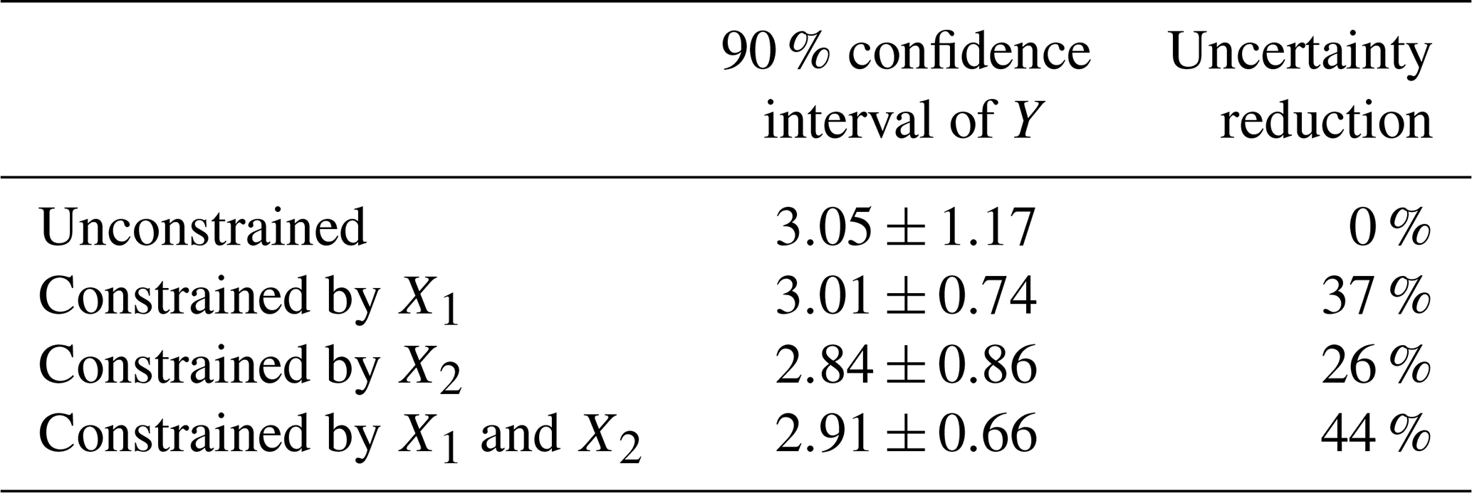
Compared with the case with no constraints, both X₁ and X₂ help to reduce the uncertainty by 37 % and 26 %, respectively (see Table I1), due to their high inter-model correlations with Y (0.78 and 0.68, respectively). The difference in uncertainty reduction is mainly due to the difference in correlation. There is also a difference in the constrained guess obtained using X₁ or X₂. This is due to the difference between the observation and multi-model mean, which is smaller for X₁ than for X₂, see Fig. I1. In summary, ClimLoco1.0 is sensitive to the choice of X. This influences the results depending on the correlation between X and Y, as well as the difference between the multi-model mean and the observation of X.

Using both X₁ and X₂ to constrain Y results in an even stronger uncertainty reduction (44 %) and the constrained guess lies between those obtained using only X₁ and X₂ individually. This illustrates the advantage of using a multivariate approach: the additional information gained helps to reduce uncertainty further and obtain a more balanced result by considering more data.

I2 Comparison with the literature

The main part of the article compares two types of approach to ClimLoco1.0 from a mathematical point of view. The first is based on the work of Bowman et al. (2018) and the second on that of Cox et al. (2018). We compare ClimLoco1.0 and these two methods when Y is constrained by X₁ (see the previous section). The resulting confidence intervals are shown in the first row of Table I2. Because there are many climate models and a high signal-to-noise ratio (i.e. low observational noise), there are few differences between the three results. To demonstrate the advantages of our method of rigorously accounting for uncertainty arising from the limited number of climate models and observational noise, we reduce the number of climate models considered (second row) and increase the observational noise (third row).

Table I2 The 90 % confidence interval of Y, the mean anomaly of GSAT between 2081 and 2100, is constrained by X₁, the mean anomaly of GSAT between 2015 and 2024. The reference period is 1850–1900. The columns correspond to the various methods employed to estimate the confidence interval. The first row was obtained using the original data. The second row uses a subset of five climate models selected from the original 32. The third row virtually increases the observational noise variance (by decreasing the signal-to-noise ratio, SNR). The bold values in each column highlight the impact of the dataset on each method in term of uncertainties.

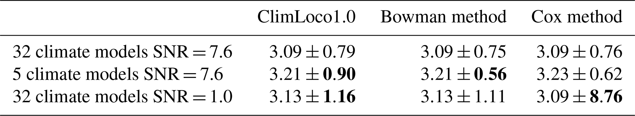
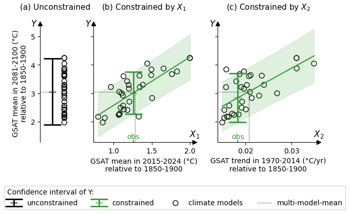
Figure I1 Illustration of different constraints on the future global mean surface air temperature (GSAT). Y, the GSAT 2081–2100 mean anomaly, is either (a) unconstrained, (b) constrained by the GSAT 2015–2024 mean anomaly, or (c) constrained by the GSAT 1970–2014 trend anomaly. The confidence intervals are displayed at a confidence level of 90 %.

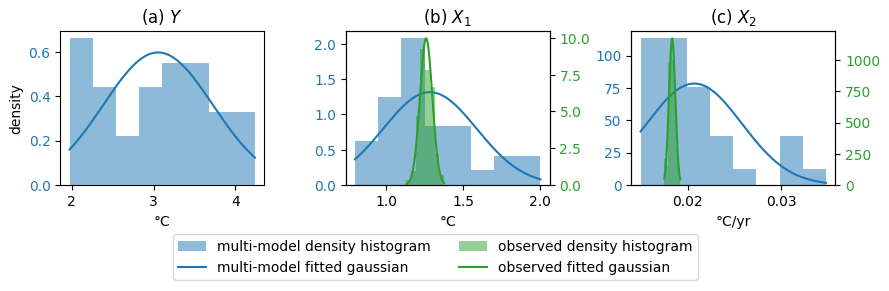
Figure I2 Comparison between the histograms and Gaussian distributions for different variables. Y is the 2081–2100 mean GSAT anomaly. The reference period is 1850–1900. X₁ is the 2015–2024 mean GSAT anomaly. X₂ is the 1970–2014 trend of GSAT anomaly. The blue histograms show the results from the 32 climate models. The green histograms show the results from 200 members of the HadCRUT5 reanalysis.

Compared with ClimLoco1.0, Bowman et al. (2018) method does not consider uncertainties arising from the limited number of climate models. Consequently, its total uncertainty is always lower than the total uncertainty in ClimLoco1.0 (column 1 vs. 2 in Table I2), especially when there are few climate models (second row).

When the observational noise is 10 times stronger than the inter-model spread (SNR = 0.1), as in the third row of Table I2, the observation is very poorly used in ClimLoco1.0. Indeed, the constrained result is very close to the unconstrained one (3.13±1.16 vs. 3.05±1.17, respectively). The constraint is attenuated by the observational noise, as explained in the main text Sect. 4. The method from Cox et al. (2018) does not attenuate the constraint by the observational noise. It considers the observation the same regardless of whether it is of good or bad quality. In this high observational-noise case, it results in a very strong uncertainty (3.09±8.76).

To summarise, this test illustrates what is demonstrated in the mathematical comparison of methods (Sect. 5). When the number of climate models is low and/or the observational noise is high, it is important to rigorously consider the uncertainties arising from these two sources.

I3 Test if the distributions are Gaussian

One of the assumptions used in the article is that the distributions are Gaussian. Figure I2 shows the density histograms for the realisations of X₁, X₂, and Y. These are compared with Gaussian distributions with the same mean and variance. The histograms of the 200 members of HadCRUT 5 are close to Gaussian distributions for these variables. However, this is not the case for the histograms of climate models. The Gaussian assumption does not appear to be verified here, resulting in deformed confidence intervals. Improving ClimLoco to enable consideration of other distributions is a promising perspective.