Tuning parameters of a sea ice model using machine learning

We developed a new method for tuning sea ice rheology parameters, which consists of two components: a new metric for characterising sea ice deformation patterns and a machine learning (ML)-based approach for tuning rheology parameters. We applied the new method to tune the brittle Bingham–Maxwell rheology (BBM) parameterisation, which was implemented and used in the next-generation sea ice model (neXtSIM). As a reference dataset, we used sea ice drift and deformation observations from the RADARSAT Geophysical Processing System (RGPS).

The metric characterises a field of sea ice deformation with a vector of values. It includes well-established descriptors such as the mean and standard deviation of deformation, the structure–function of the spatial scaling analysis, and the density and intersection of linear kinematic features (LKFs). We added more descriptors to the metric that characterises the pattern of ice deformation, including image anisotropy and Haralick texture features. The developed metric can describe ice deformation from any model or satellite platform.

In the parameter tuning method, we first run an ensemble of neXtSIM members with perturbed rheology parameters and then train a machine learning model using the simulated data. We provide the descriptors of ice deformation as input to the ML model and rheology parameters as targets. We apply the trained ML model to the descriptors computed from RGPS observations. The developed ML-based method is generic and can be used to tune the parameters of any model.

We ran experiments with tens of members and found optimal values for four neXtSIM BBM parameters: scaling parameter for compressive strength (P₀≈5.1 kPa), cohesion at the reference scale (c_ref≈1.2 MPa), internal friction angle tangent (μ≈0.7) and ice–atmosphere drag coefficient (C_A≈0.00228). A neXtSIM run with the optimal parameterisation produces maps of sea ice deformation visually indistinguishable from RGPS observations. These parameters exhibit weak interannual drift related to changes in sea ice thickness and corresponding changes in ice deformation patterns.

1 Introduction

Sea ice dynamics in highly compact ice result from the interaction between surface stress on the ice supplied by wind and ocean currents and the emerging internal stress in the ice. In sea ice models, the internal stress is calculated by a set of equations commonly referred to as rheology. Virtually all large-scale sea ice models used for sea ice forecasting and climate modelling use the so-called viscous–plastic (VP) rheology of Hibler (1979) or more numerically efficient derivatives thereof. Additionally, the elastic–plastic–anisotropic (EAP) approach was introduced by parameterising the anisotropy of the ice stress through interactions of diamond-shaped floes (e.g. Tsamados et al., 2013; Wilchinsky and Feltham, 2004). The free parameters of the VP rheology have been estimated in various traditional sensitivity experiments (e.g. Panteleev et al., 2020, 2023), and their values are generally considered fixed by the community today.

A new branch of brittle rheologies has been proposed and extended by Girard et al. (2011), Dansereau et al. (2016) and Ólason et al. (2022), with the latest version, i.e. the brittle Bingham–Maxwell (BBM) rheology, implemented and used in the next-generation sea ice model (neXtSIM) (e.g. Rampal et al., 2016, 2019); neXtSIM, with the BBM rheology, has already been used in several scientific studies (e.g. Boutin et al., 2022, 2023; Korosov et al., 2023; Regan et al., 2023) and is used for operational sea ice forecasts (Williams et al., 2021), and the BBM rheology has been implemented in SI3, i.e. the sea ice component of the NEMO model (Brodeau et al., 2024). However, the free parameters of the BBM rheology have only been briefly explored, and their range and relation to other model components and parameters remain unclear.

The BBM rheology, like the other brittle rheologies, is a damage-propagation model. It parameterises the density of fractures (the mechanical weakness of sea ice) at the subgrid scale with a scalar damage variable. In this framework, undamaged ice is fully elastic, and damage increases when the local stresses reach the Mohr–Coulomb failure criterion. An increase in damage results in a decrease in elasticity, simulating the fracturing of the ice. Once fractured, the ice can also deform viscously, simulating the permanent deformation of fractured ice. This permanent viscous deformation is limited in convergence by resistance to ridge formation, which is also accounted for by the BBM rheology.

As pointed out in Ólason et al. (2022), the BBM rheology has many parameters, with some well-defined constants and some poorly constrained. These parameters strongly and nonlinearly impact the patterns of sea ice drift and deformation simulated by the model. Visually, the differences between observed and simulated deformation fields can guide the selection of a model parameter value. Still, such manual tuning can become complicated when several parameters must be considered. This work aims to develop a set of metrics for quantitative comparison of the simulated and observed sea ice deformation fields and to use these metrics for tuning BBM parameters utilising a deep learning approach.

2 A brief introduction to the BBM rheology

The constitutive model of the BBM rheology consists of a parallel dashpot and a friction element, connected in series with a spring (see Fig. A1). The spring represents elastic ice deformation, the dashpot represents viscous deformation when the ice is fractured and the friction element represents the resistance of broken ice to ridge formation. In a simple 1D case, these regimes can be summarised as follows (with σ, σ_E and σ_v denoting total, elastic and viscous internal stresses, and ε, ε_E and ε_v denoting total, elastic and viscous deformations). Note that due to the serial connectivity, the elastic stress always equals the total stress, i.e. σ_E=σ.

• When sea ice is undamaged, viscous stress is zero, and total deformation is fully reversible (elastic): d=0, σ_v=0 and ε=ε_E, where damage is a single scalar to parameterise the fracture density at the subgrid scale. The damage value is altered whenever the local stress exceeds the Mohr–Coulomb failure criterion.

• When ice is damaged and diverging, the friction element is inactive; therefore, the viscous stress equals the elastic and total stress. Deformation is both elastic and viscous: d>0, σ>0, ${\mathit{\sigma }}_{\mathrm{v}}={\mathit{\sigma }}_{\mathrm{E}}=\mathit{\sigma }$ and $\mathit{\epsilon }={\mathit{\epsilon }}_{\mathrm{E}}+{\mathit{\epsilon }}_{\mathrm{v}}$.

• When ice is damaged and converging with weak internal stress, the friction element is active, viscous stress is zero and all deformations are elastic. d>0, $P_{max}<\mathit{\sigma }<\mathrm{0}$, σ_v=0 and ε=ε_E, where P_max is a compressive ice strength threshold that separates the elastic behaviour from the elastic and stress-dissipative behaviour of damaged sea ice.

• When ice is damaged and converging with strong internal stresses, the friction element is inactive; therefore, the viscous stress is equal to the elastic and total stress, and deformation is both elastic and viscous: d>0, $\mathit{\sigma }<P_{max}$, ${\mathit{\sigma }}_{\mathrm{v}}=\mathit{\sigma }-P_{max}$ and $\mathit{\epsilon }={\mathit{\epsilon }}_{\mathrm{E}}+{\mathit{\epsilon }}_{\mathrm{v}}$.

Accounting for two components of the internal stress tensor (normal stress, σ_N, and tangent stress, τ), we can generalise the equation for the viscous stress as follows:

$$\begin{array}{}\text{(1a)}& {\displaystyle }{\mathit{\sigma }}_{\mathrm{v}}& {\displaystyle }=(\mathrm{1}+\stackrel{\mathrm{̃}}{P})\mathit{\sigma };\text{(1b)}& {\displaystyle }\stackrel{\mathrm{̃}}{P}& {\displaystyle }=\left\{\begin{array}{ll}\frac{P_{max}}{{\mathit{\sigma }}_N}& \text{ for }{\mathit{\sigma }}_N<-P_{max},\\ -\mathrm{1}& \text{ for }-P_{max}<{\mathit{\sigma }}_N<\mathrm{0},\\ \mathrm{0}& \text{ for }{\mathit{\sigma }}_N>\mathrm{0},\end{array}\right.\end{array}$$

where the threshold P_max separates the elastic and viscoelastic regimes and can be computed following the results of Hopkins (1998) and Hibler (1979):

$$\begin{array}{}\text{(2)}& P_{max}=P_{\mathrm{0}}{\left({\displaystyle \frac{h}{h_{\mathrm{0}}}}\right)}^H{e}^{C(\mathrm{1}-A)},\end{array}$$

where h is sea ice thickness, h₀=1 m is a constant reference thickness, $H=\mathrm{3}/\mathrm{2}$ is the exponent of the compression factor, P₀ is a constant reference stress, C<0 is compaction parameter and A is ice concentration.

The time derivative of total stress (see details in Ólason et al., 2022) is

$$\begin{array}{}\text{(3)}& \dot{\mathit{\sigma }}=E\mathit{K}:\dot{\mathit{\epsilon }}-{\displaystyle \frac{\mathit{\sigma }}{\mathit{\lambda }}}\left(\mathrm{1}+\stackrel{\mathrm{̃}}{P}+{\displaystyle \frac{\mathit{\lambda }\dot{d}}{\mathrm{1}-d}}\right),\end{array}$$

where elasticity is a function of damage and concentration:

$$\begin{array}{}\text{(4)}& E=E_{\mathrm{0}}(\mathrm{1}-d)e^{C(\mathrm{1}-A)}.\end{array}$$

$\mathit{K}:\dot{\mathit{\epsilon }}$ is the stiffness tensor operation:

$$\begin{array}{}\text{(5)}& \left(\begin{array}{c}(\mathit{K}:\dot{\mathit{\epsilon }}{)}_{\mathrm{11}}\\ (\mathit{K}:\dot{\mathit{\epsilon }}{)}_{\mathrm{22}}\\ (\mathit{K}:\dot{\mathit{\epsilon }}{)}_{\mathrm{12}}\end{array}\right)={\displaystyle \frac{\mathrm{1}}{\mathrm{1}-{\mathit{\nu }}^{\mathrm{2}}}}\left(\begin{array}{ccc}\mathrm{1}& \mathit{\nu }& \mathrm{0}\\ \mathit{\nu }& \mathrm{1}& \mathrm{0}\\ \mathrm{0}& \mathrm{0}& \mathrm{1}-\mathit{\nu }\end{array}\right)\left(\begin{array}{c}{\dot{\mathit{\epsilon }}}_{\mathrm{11}}\\ {\dot{\mathit{\epsilon }}}_{\mathrm{22}}\\ {\dot{\mathit{\epsilon }}}_{\mathrm{12}}\end{array}\right),\end{array}$$

where λ is the viscous relaxation time:

$$\begin{array}{}\text{(6)}& \mathit{\lambda }={\mathit{\lambda }}_{\mathrm{0}}(\mathrm{1}-d{)}^{\mathit{\alpha }-\mathrm{1}},\end{array}$$

with E₀ (undamaged elasticity), ν (Poisson's ratio), λ₀ (undamaged viscous relaxation time) and α>0 being constants.

Damage occurs in the BBM rheology whenever the simulated stress in a grid cell or element is outside the failure envelope (or yield curve). The failure envelope of the BBM rheology is the Mohr–Coulomb criterion:

$$\begin{array}{}\text{(7)}& \mathit{\tau }=\mathit{\mu }{\mathit{\sigma }}_N+c,\end{array}$$

where μ is the internal friction coefficient, and c is the cohesion. Following Bouillon and Rampal (2015), we let the cohesion scale with model resolution as

$$\begin{array}{}\text{(8)}& c\sim c_{\text{ref}}\sqrt{{\displaystyle \frac{l_{\text{ref}}}{\mathrm{\Delta }x}}},\end{array}$$

where Δx is the distance between model node points, and c_ref is the cohesion at the reference length scale, i.e. l_ref=10 cm, where the cohesion was measured to be of the order of 1 MPa (Schulson et al., 2006).

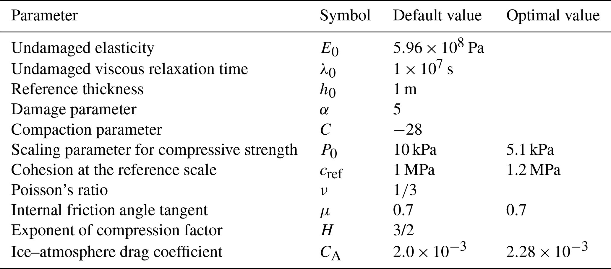
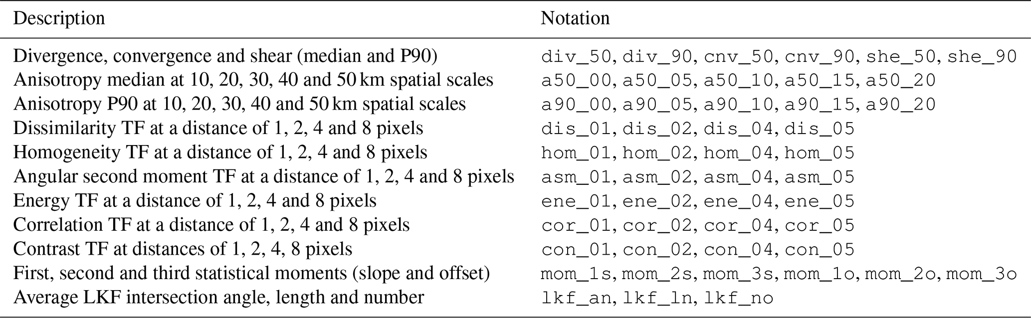
The aforementioned parameters of the neXtSIM BBM rheology are summarised in Table 1. The ice–atmosphere drag coefficient C_A is also added to the table (although, strictly speaking, it is not a rheology parameter) as it controls the amount of energy transferred from wind and ocean to sea ice and strongly affects the sea ice drift speed and, respectively, sea ice deformation. According to Ólason et al. (2022), such parameters as P₀ and c_ref require tuning using satellite observations at large spatial and temporal scales. Given that the rheology parameters nonlinearly affect the field of sea ice deformation, a metric based on satellite-derived deformation should be used, and the tuning should capitalise on nonlinear methods, such as deep learning.

Table 1 The default and optimised (see Sect. 5.4) parameters of the BBM rheology.

3 Data

We used the Lagrangian sea ice motion data from the RADARSAT Geophysical Processing System (RGPS) (Kwok et al., 2008) for tuning the above rheology parameters. The dataset contains trajectories of virtual buoys tracked using pattern-matching techniques on synthetic aperture radar (SAR) imagery from RADARSAT-2. The buoys are initialised by the RGPS in mid-December in the western Arctic on a regular grid with 10 km spacing on individual SAR images. The position of each virtual buoy is tracked from one image to another overlapping image during the entire winter season (December–May). The trajectory is terminated if a virtual buoy cannot be tracked due to a loss of similarity between SAR images or the absence of images. New virtual buoys are initialised in the regions with a low density of the tracked buoys that appear due to sea ice divergence or disappearance of older buoys. The average time between overlapping RADARSAT-2 image acquisitions is 3 d, but it may vary from 0.5 to 10 d. Therefore, the timing of virtual buoy positions is highly heterogeneous, even for neighbour trajectories (see Appendix A for details).

4 Methodology

4.1 Overview of the parameter tuning algorithm

In our approach, we compute a set of descriptors that characterise patterns in the fields of observed and simulated sea ice deformation. Since the correlation between the descriptors and model parameters is weak (see Fig. 6), we could not use linear-regression-based methods (e.g. Ensemble Kalman filter; Massonnet et al., 2014; Zhang et al., 2021; Chen et al., 2024) and chose a deep learning (DL) approach instead. In our DL approach for tuning the neXtSIM parameter values, we train a neural network based on the modelling results and apply it to actual observations. The inputs for the neural network are the descriptors of the sea ice deformation, and the target is a value of a rheological parameter.

The algorithm for DL parameter tuning can be summarised as follows:

1. We choose the neXtSIM rheology parameters for tuning and perturb their values to generate an ensemble. Let ϕ_m,n denote the mth parameter for the nth member of the ensemble, then ϕ_m denotes a vector of the mth parameter for all members.

2. An ensemble of neXtSIM instances is run with the same forcings but with different rheology parameters:

   $$\begin{array}{}\text{(9)}& {\stackrel{\mathrm{̃}}{\mathit{x}}}_{n,t+\mathrm{1}}=\mathcal{M}(t,{\stackrel{\mathrm{̃}}{\mathit{x}}}_{n,t};{\mathit{\varphi }}_n),\end{array}$$

   where $\stackrel{\mathrm{̃}}{\mathit{x}}$ is the sea ice model state (sea ice concentration, thickness, drift, etc.), ℳ is neXtSIM and t is time.

3. Let x denote only one model variable: sea ice drift. Then ℋ denotes the operator for computing a sea ice deformation field and a quantitative characterisation of ice deformation pattern y:

   $$\begin{array}{}\text{(10)}& {\mathit{y}}_{n,t}=\mathcal{H}\left({\mathit{x}}_{n,t}\right).\end{array}$$

   The size of y_n,t is much smaller than the ice deformation field. For example, a daily deformation field containing ∼10¹⁰ sea ice deformation values can be characterised by a vector with ∼50 values.

4. Let y denote a set of y_n,t vectors from all members and all time steps. Hereafter, y represents the deformation pattern descriptors or simply descriptors. A neural network 𝒩 is trained (operator 𝒯) with the deformation pattern descriptors (y) as input and the rheology parameters (ϕ_m) as the target:

   $$\begin{array}{}\text{(11)}& {\mathcal{N}}_m=\mathcal{T}(\mathit{y},{\mathit{\varphi }}_m).\end{array}$$

5. Deformation fields and deformation pattern descriptors are computed from the observed sea ice drift x^o for each time step t:

   $$\begin{array}{}\text{(12)}& {\mathit{y}}_t^{\mathrm{o}}=\mathcal{H}\left({\mathit{x}}_t^{\mathrm{o}}\right).\end{array}$$

6. The neural network is applied to the deformation pattern descriptors computed from the observed ice drift, and averaging (〈〉) is applied for computing the optimal value of a neXtSIM parameter:

   $$\begin{array}{}\text{(13)}& \begin{array}{r}{\displaystyle }{\mathit{\varphi }}_{m,t}^{\mathrm{o}}={\mathcal{N}}_m\left({\mathit{y}}_t^{\mathrm{o}}\right)\\ {\displaystyle }{\mathit{\varphi }}_m^{\mathrm{o}}=\langle {\mathit{\varphi }}_{m,t}^{\mathrm{o}}\rangle .\end{array}\end{array}$$

All these steps are described in detail below.

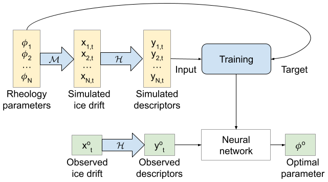
Figure 1 Scheme of machine learning (ML)-based tuning of neXtSIM parameters. Blue arrows denote operations with data. Yellow squares denote modelling data. Green squares denote observations. The operators ℳ and ℋ denote, respectively, neXtSIM simulations and computation of sea ice deformation descriptors.

4.2 Running an ensemble of neXtSIM instances

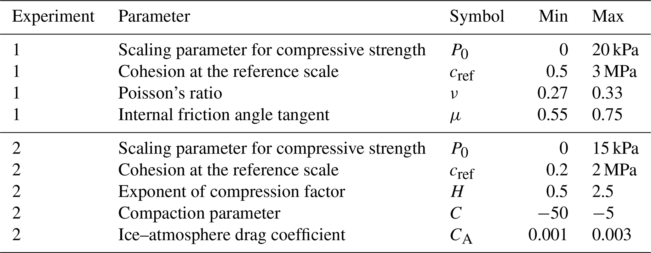
We ran two ensembles with neXtSIM instances. In the first experiment, the ensemble consisted of 50 members, and the values of four parameters were perturbed using the Latin hypercube method (McKay et al., 1979): P₀, c_ref, ν and μ. In the second experiment with 70 members, the following parameters were perturbed with the same method: P₀, c_ref, H, C and C_A. The H and C parameters were added as they control the influence of sea ice thickness on P_max. See the ranges of the perturbed parameters in Table 2.

Table 2 Ranges of parameters perturbed in two experiments.

The neXtSIM instances were run at a 10 km resolution mesh, covering the central Arctic Ocean. Ocean forcing from the TOPAZ4 reanalysis (Sakov et al., 2012) and atmosphere forcing from the ERA5 reanalysis (Hersbach et al., 2020) were used; neXtSIM exports snapshot outputs every hour with coordinates and connectivity of the nodes of the triangular mesh and model variables for each mesh element, including ice concentration, thickness, etc. End-to-end indexing of the model nodes allows for the identification of similar nodes on two snapshots and the computation of the displacement of the node, i.e. the simulated sea ice drift.

4.3 Preprocessing of neXtSIM data

To ensure comparability of sea ice drift and deformation from RGPS and neXtSIM, we subsample the model mesh using the mesh of satellite observations. First, for a given set of virtual RGPS buoys that have the same starting time and ending time (i.e. a single pair of SAR images is used for ice drift computation for these buoys), two model snapshots with the closest simulation time are selected from the neXtSIM outputs. Next, only the neXtSIM nodes near the RGPS nodes are selected on the first snapshot, and the corresponding nodes are chosen on the second snapshot (see Fig. A3 for an example). Nodes may disappear during simulation, or new nodes map appear due to convergence/divergence and consequent remeshing. In that case, a new Delaunay triangulation connectivity is computed between the nodes existing on the first and second snapshots. Further drift, deformation and descriptor calculations are performed on subsets of trajectories (same for RGPS or neXtSIM) with the same start and end times. They are somewhat limited in space (by the intersection area of two SAR images).

4.4 Computing the descriptors of the sea ice deformation

We compute the divergence and shear components of the deformation tensor and the total deformation rates using a standard method of contour integrals of velocity (Kwok, 2006) for each element of the mesh subset mentioned above. The following descriptors of the total deformation field are computed from each subset as described in the subsections below:

1. structure–function from the spatial scaling analysis;

2. image anisotropy at different spatial scales;

3. Haralick texture features at different spatial scales;

4. length, density, and angle of intersection of linear kinematic features (LKFs); and

5. mean and 90th percentile of ice deformation values.

4.4.1 Spatial scaling analysis

As described in Ólason et al. (2022), the deformation is computed at different spatial scales by iterative coarse-graining (Marsan and Weiss, 2010). First, the deformation is calculated on the native resolutions of RGPS and neXtSIM (which are very similar). Next, some nodes are randomly removed, the remaining node positions are triangulated, and deformation is computed again. The last step is repeated several times until at least three nodes remain in the subset. Information about the area of the element used for computing deformation is preserved. This iterative procedure is repeated several times, starting from the initial deformation field, to collect sufficient deformation observations computed at different spatial scales.

The spatial scale L is linked with the statistical moments Q of the total deformation probability density function using the following equation:

$$\begin{array}{}\text{(14)}& L_{\lg }={\mathit{\alpha }}_N+{\mathit{\beta }}_N{Q}_{\lg }^N,\end{array}$$

where α and β are coefficients found using the least squares method, N is the statistical moment order, and the subscript “lg” indicates logarithmic space. The Nth statistical moment is computed as $Q_{\lg }^N=\langle {\log }_{\mathrm{10}}\left(\right(\mathit{\epsilon }-\widehat{\mathit{\epsilon }}{)}^N)\rangle$, where $\widehat{\mathit{\epsilon }}$ is mean total deformation and 〈〉 denotes averaging.

Coarse-graining is performed on each deformation subset (see Sect. 3.3). Still, the α and β coefficients are computed using deformation values (and corresponding spatial scales) from all image pairs acquired within 3 d. Hereafter, the offset and scale of the first statistical moment are denoted mom_1o and mom_1s, respectively (and so on) (see Table 3).

4.4.2 Image anisotropy

Image anisotropy a_I characterises localisation of image intensity in a linear feature (Lehoucq et al., 2015). Anisotropy is high (up to 1) for images of bright, thin or long lines and is low (down to 0) for images with dark, thick or short lines. We compute the image anisotropy as

$$\begin{array}{}\text{(15)}& a_{\mathrm{I}}=\mathrm{1}-\sqrt{{\displaystyle \frac{{\mathit{\lambda }}_{\mathrm{1}}}{{\mathit{\lambda }}_{\mathrm{2}}}}},\end{array}$$

where λ₁ and λ₁ are the eigenvalues of the inertia matrix P:

$$\begin{array}{}\text{(16)}& \mathbf{P}=\sum _{\mathrm{box}}\left(\begin{array}{cc}{\mathit{X}}^{\mathrm{2}}& \mathit{X}\mathit{Y}\\ \mathit{X}\mathit{Y}& {\mathit{Y}}^{\mathrm{2}}\end{array}\right)\mathit{I},\end{array}$$

where X and Y are coordinates of the pixels of the image with intensities I (i.e. ice deformation in our case).

In our study, anisotropy is computed on triangular mesh elements as illustrated in Fig. 2. Only elements with deformation above 0.1 d⁻¹ are used to avoid the impact of noise in sea ice drift and deformation (Dierking et al., 2020). For computing a_I in a selected element, the nearest-neighbour elements are found, and values of deformation and the coordinates of the centres of the elements are used in Eqs. (15) and (16) (see Fig. 2, left column). For larger spatial scales (Fig. 2, second, third and fourth columns), values of the deformation and coordinates are collected from the neighbours of the neighbours. After processing a single mesh subset, each element is characterised by a vector of image anisotropy computed at spatial scales of 10, 20, 30, 40 and 50 km. For every 3 d, a median and 90th percentile (P90) of anisotropy from all elements of all mesh subsets are computed for each spatial scale and denoted hereafter as a50_00, a90_00 and so on (see Table 3).

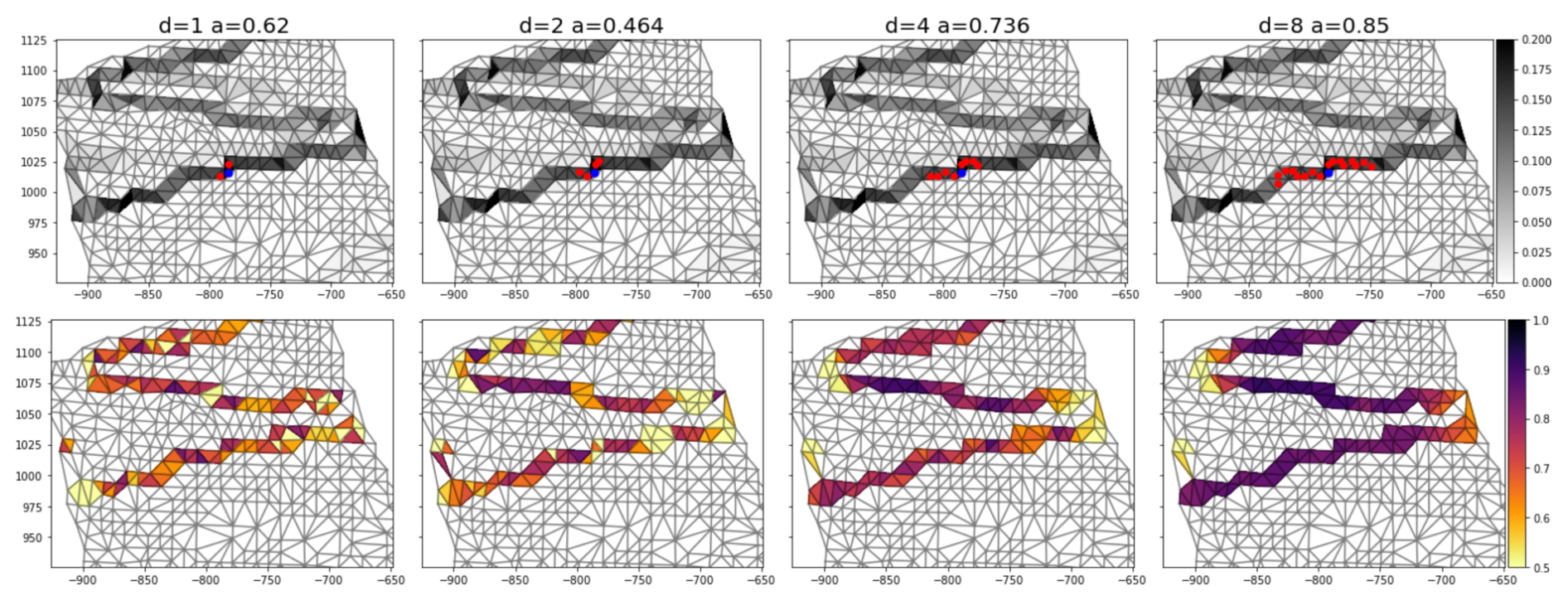
Figure 2 Computation of image anisotropy on a mesh subset. The upper row shows a mesh subset with values of ice deformation (d⁻¹), and the lower row shows values of anisotropy computed at different spatial scales. The blue dot on the upper row shows the location of an arbitrary element for which anisotropy was computed, and the red dots show the neighbours from which the deformation and coordinates were collected.

4.4.3 Texture features

Haralick texture features (TFs) are extensively used for quantitative characterisation of image texture in tasks dealing with image segmentation (Haralick et al., 1973; Zakhvatkina et al., 2017; Park et al., 2020). A grey-level co-occurrence matrix (GLCM) is computed at the first stage of the texture analysis. The GLCM is a 2D distribution of the probability of a pixel value and its neighbour value. The neighbours can be selected at varying orientations and distances from the central pixel. At the second stage of texture analysis, several simple algebraic formulas are applied to the GLCM to compute statistical moments of the distribution (mean, standard deviation, kurtosis, etc.) and more complex characteristics (energy, entropy, etc.).

In our study, we compute the GLCM from the triangular mesh elements. We accumulate information about an element and all its neighbours at a given distance in all directions in one GLCM. For one-edge distance, we use the values from three immediate neighbours; for two-edge distances, we use the values from neighbours of neighbours (excluding the central element and duplication), and so on, as shown in Fig. 3. We populate the GLCM with data from all elements from all mesh subsets acquired within 3 d. The following TFs are computed at distances of 1, 2, 4 and 8 edges using the scikit-image Python library (van der Walt et al., 2014): dissimilarity, homogeneity, angular second moment, energy, correlation and contrast. For the notation, see Table 3. Zakhvatkina et al. (2017) provides the exact formulas.

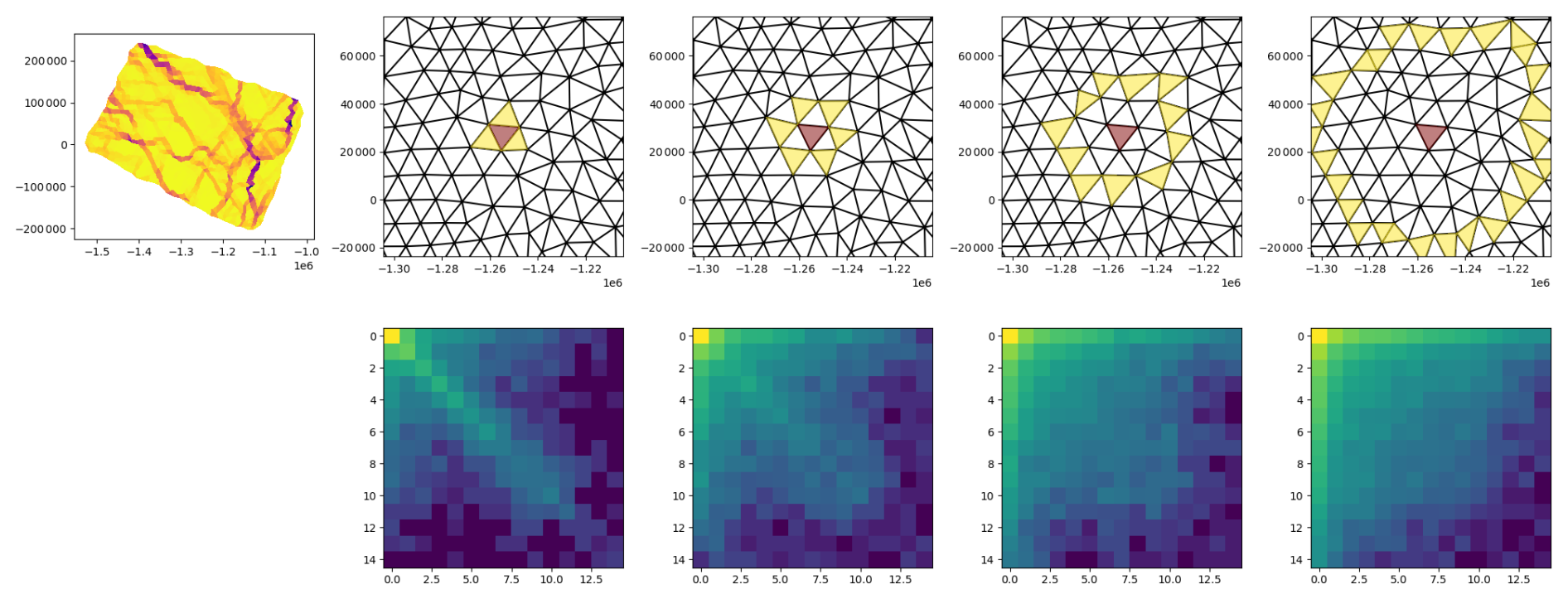
Figure 3 Scheme of the GLCM computation. The upper left map shows a mesh subset with values of total deformation from neXtSIM. The upper row shows the neXtSIM mesh with the central element coloured orange, and the neighbours at the one-, two-, four- and eight-edge distances are coloured yellow. The lower row of images shows corresponding GLCMs.

4.4.4 LKF intersection angle

Hutter et al. (2019) proposed a method for detecting linear kinematic features (LKFs) for RGPS and model data as well as several metrics for the characterisation of LKFs. These metrics are successfully applied to evaluate sea ice models in a large intercomparison experiment (Hutter and Losch, 2020). In our work, we rasterised the 3 d deformation maps on 12.5 km resolution grids and applied the LKF detection method of Hutter et al. (2019). The number of LKFs, average length of LKFs and average intersection angle of conjugate faults were used as the descriptors (see Table 3 for notation).

In addition to the descriptors listed above, the median and P90 of divergence, convergence, and shear were computed for each of the 3 d. Thus, a vector of descriptors constituted 49 values: median and P90 of deformation; median and P90 of image anisotropy computed at five spatial scales; six texture features at four distances; slopes and offsets of three statistical moments; and length, number, and intersection of LKFs. Table 3 shows the notation used hereafter in detail. Such vectors were generated from neXtSIM simulations for each day (using a sliding window of 3 d) from 5 December 2006 to 11 April 2007 for the first experiment and from 5 December 2006 to 15 May 2007 for the second experiment. Therefore, we had $\mathrm{127}\times \mathrm{50}=\mathrm{6350}$ and $\mathrm{161}\times \mathrm{70}=\mathrm{11}\mathrm{270}$ vectors for training the ML model in the first and second experiments.

Table 3 Descriptor notation.

4.5 Selection of usable descriptors

We test the applicability of these descriptors in two steps: on the one hand, we compare probability density functions (PDFs) for descriptors from RGPS and neXtSIM, and on the other hand, we use an autoencoder. In the first step, we scale the values of descriptors from the RGPS using the mean and standard deviation of the values from neXtSIM: $y_s=(y_o-\mathit{\mu })/\mathit{\sigma }$, where y_o represents all descriptors from the RGPS, and μ and σ are the mean and standard deviation, respectively, for all descriptors from neXtSIM.

The mean and standard deviation of the scaled descriptors are analysed, and only the descriptors with scaled standard deviation below 3 remain for further use. Six descriptors computed from RGPS data have significantly different values from the neXtSIM descriptors and are expected to mislead the training.

We trained an autoencoder (Hinton and Salakhutdinov, 2006; Vincent et al., 2008) with dense layers with 32, 16, 8, 16 and 32 neurons on the down-selected descriptors from neXtSIM. Due to the bottleneck, the autoencoder acts as a nonlinear principal component analysis. It can be used for anomaly detection either in the input features (Hinton and Salakhutdinov, 2006) or in input records (Vincent et al., 2008). We applied the autoencoder to the down-selected neXtSIM and RGPS descriptors and computed the root-mean-square difference (RMSD) between the input vector and the autoencoder output for neXtSIM and the RGPS. We excluded seven descriptors with high RMSE in RGPS data from further processing as these are anomalous compared to neXtSIM training data.

4.6 Training of machine learning algorithms

We trained two types of ML models with the values of deformation pattern descriptors as input and a single value of a neXtSIM parameter as a target: a linear regression (LR) model and a deep neural network (DNN). For both models, we split the dataset from neXtSIM into two parts (85:15) for training and validation. Training and validation data are taken from different months (selected randomly). The models are trained on neXtSIM data and then applied to all RGPS descriptors. We repeated this procedure 10 times with a new random permutation and averaged the inference results on the RGPS from each repetition. Eqs. (11) and (13) can be rewritten as follows with i being the index of repetition:

$$\begin{array}{}\text{(17a)}& {\displaystyle }{\mathcal{N}}_{m,i}& {\displaystyle }=\mathcal{T}({\mathit{y}}_{\mathit{i}},{\mathit{\varphi }}_{m,i}),\text{(17b)}& {\displaystyle }{\mathit{\varphi }}_{m,t,i}^{\mathrm{o}}& {\displaystyle }={\mathcal{N}}_{m,i}\left({\mathit{y}}_t^{\mathrm{o}}\right),\text{(17c)}& {\displaystyle }{\mathit{\varphi }}_m^{\mathrm{o}}& {\displaystyle }=\langle {\mathit{\varphi }}_{m,t,i}^{\mathrm{o}}\rangle .\end{array}$$

The LR model can be formulated as

$$\begin{array}{}\text{(18)}& {\mathit{\varphi }}_p={\mathbf{A}}_p\mathbf{Y},\end{array}$$

where ϕ_p is the vector of the pth model parameter for all 3 d periods, Y is a matrix with down-selected descriptors for all periods and A_p is a matrix with linear regression coefficients for that model parameter. Values in A_p are found using the least squares method. The LR model does not require a split into training/validation datasets. However, only the training dataset was compared with the DNN results.

The DNN model contains three hidden dense layers with 32, 16 and 8 fully connected neurons. We found this architecture optimal in a simple hyperparameter tuning experiment. The hidden layers use the rectified linear unit (ReLU) activation function, and the output layer uses linear activation. We trained the DNN with the Adam optimiser (Kingma and Ba, 2017), and the validation loss (computed as absolute error) decreased.

5 Results and discussions

5.1 Sea ice deformation fields from neXtSIM

Ólason et al. (2022) identified P₀ and c_ref as two parameters of their rheology that are poorly constrained and have a substantial visual impact on the deformation fields. Figure 4 compares total sea ice deformation derived from RGPS (first column) and neXtSIM runs from the first experiments with the highest and lowest values of P₀ and c_ref. Three dates were chosen for Fig. 4 in 2007 with low (15 February), moderate (25 January) and high (3 February) deformation events. These maps illustrate that both parameters significantly affect the pattern of sea ice deformation, but their influence is manifested differently. For example, the increase in P₀ results in broader and longer LKFs with higher deformation rates. These pronounced LKFs surround quite large floes; the background deformation remains relatively low. The increase in c_ref seems to affect the background deformation more – at the lowest c_ref value, the deformation between the main LKFs is mostly zero, and it increases with higher c_ref to become almost spatially homogeneous. Visually, it is hard to say which of these maps better matches the RGPS data, but we can use the similarity of deformation descriptors in PDFs as the metric. Nevertheless, optimisation of multiple rheology parameters is required to find the best match.

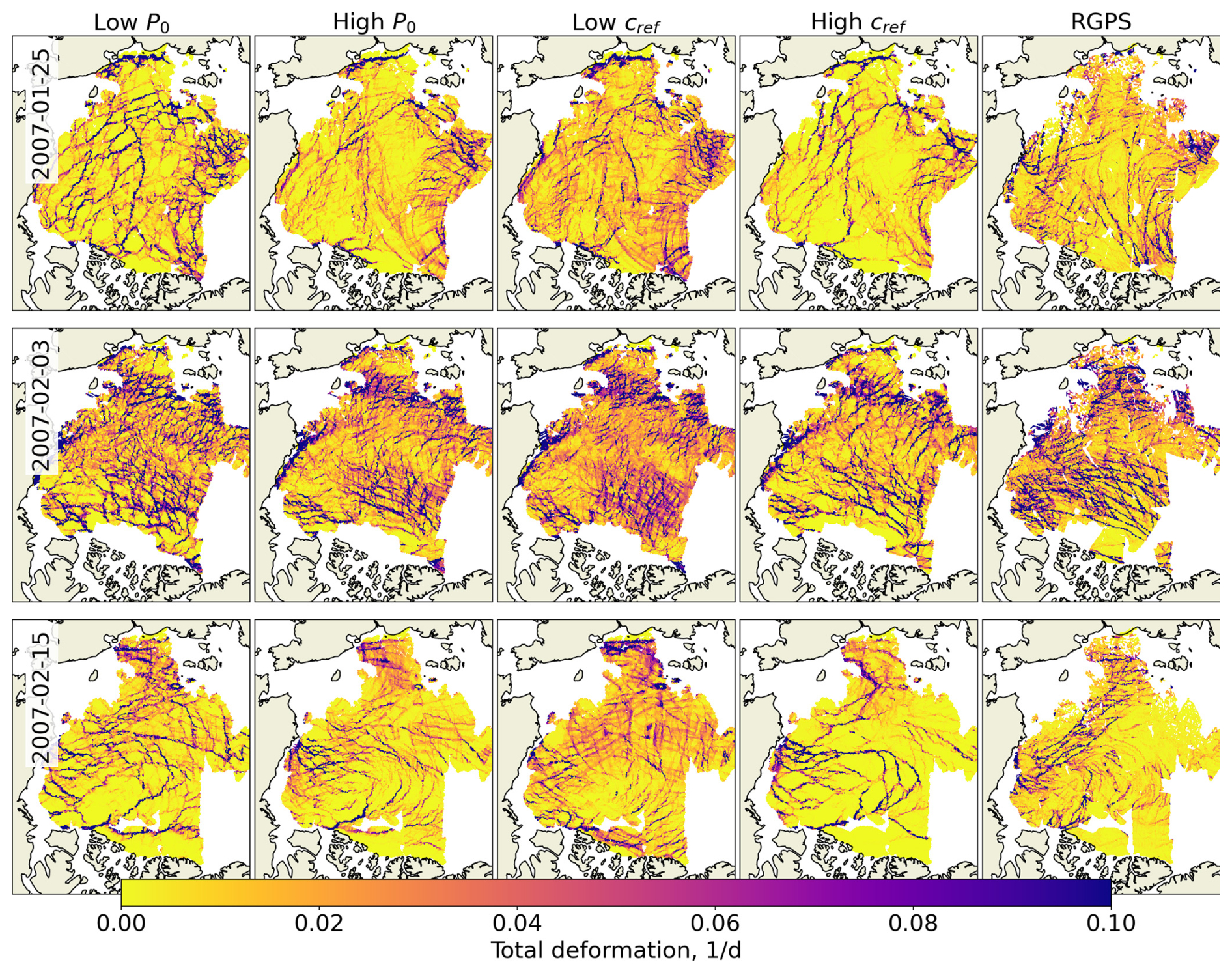
Figure 4 Maps of total deformation from RGPS and neXtSIM for three selected dates representing low, moderate and strong deformation events. Each map represents a 3 d mosaic; that is, the deformation is derived from pairs of RADARSAT-1 images (and corresponding neXtSIM snapshots) accumulated over 3 d, starting from the indicated date.

5.2 Deformation pattern descriptors

Figure 5 shows the PDFs of the deformation pattern descriptors computed from RGPS and the first neXtSIM experiment. Comparison of the PDFs from all neXtSIM runs (blue shaded area) with the PDFs from the run with the lowest (orange line) or the highest (green line) P₀ value illustrates that some descriptors (a50_00, a90_05, hom_02, con_01-08, etc.) are strongly affected by P₀ – their PDF peaks are distinctly different. Other descriptors (ASM_01-08, a50_10, etc.) have very similar PDFs without regard for the P₀ parameter. See Fig. A4 with PDFs of all deformation descriptors for reference.

The PDF of most RGPS-derived descriptors lies well within the range of neXtSIM-derived descriptors and peaks between the highest and lowest P₀ PDFs (a90_05, dis_04, mom_3o, etc.), suggesting that we can use these descriptors for parameter tuning. Some RGPS descriptors, however, show a completely different distribution (hom_08, cor_08, etc.), probably due to sensitivity to noise in observations. Such descriptors are not usable for parameter training and are excluded as described in Sect. 4.5.

Figure 6 shows the correlation of all descriptors with the values of all parameters from the first experiment. The correlations are generally relatively low, except for c_ref, which correlates with she_50 and cor_01 above 0.35. Results from the second experiment are pretty similar.

Figure 7 presents the mean and standard deviation of the RGPS-derived descriptors normalised by the mean and standard deviation of the neXtSIM descriptors. We use it at the first step of evaluating usability and selecting the descriptors. Only 43 descriptors computed from RGPS data show a relative mean value between −1.5 and 1.5 standard deviations of the neXtSIM descriptors. We exclude the following six descriptors from further processing: cor_08, a50_08, cor_01, ene_08, dis_08 and hom_08. The standard deviation of the RGPS descriptor a90_00 is very large compared to neXtSIM due to noise in the RGPS observations of ice drift and deformation (see Fig. 3, left panel).

Figure 8 compares root-mean-square difference (RMSD) between input and predictions of the autoencoder trained on normalised neXtSIM data and applied to neXtSIM and RGPS descriptors. The RMSD of neXtSIM-derived descriptors is below 1, showing that even a relatively shallow autoencoder (five layers with eight neurons in the bottleneck) can reproduce the variability of the descriptors well. When the same autoencoder is applied to the RGPS data, some of the descriptors (cnv_90, con_08, lkf_ln, lkf_no, a90_20, lkf_an and a90_00) have RMSD higher than the maximum neXtSIM RMSD. High RMSD indicates abnormal values, and we exclude the corresponding descriptors from further training.

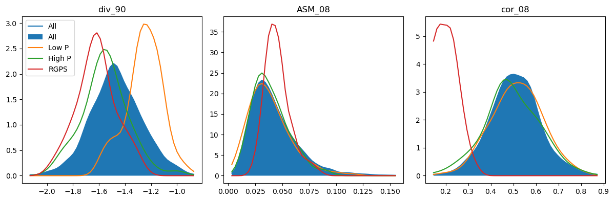
Figure 5 PDFs of a few deformation descriptors for RGPS (red), all neXtSIM runs (blue), and runs with lowest (orange) or highest values of P₀. The descriptor div_90 is promising as it shows strong sensitivity to the P₀ parameter, and the RGPS values vary within a similar range. The descriptors ASM_08 and cor_08 are less usable as they are either not sensitive to P₀ (i.e. ASM_08) or RGPS values are out of the training range (i.e. cor_08).

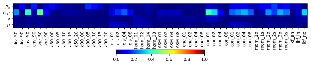
Figure 6 Correlations between four parameters of the first experiment and the deformation descriptors.

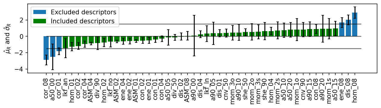
Figure 7 Relative values of the mean (shown by bar height) and standard deviation (shown by error bars) of descriptors computed from RGPS data. The blue colour shows the excluded descriptors.

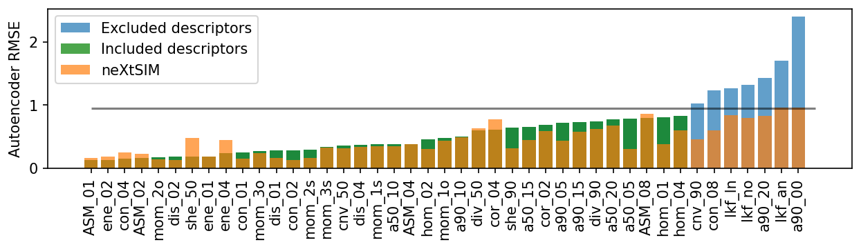
Figure 8 RMSD between input and output of the autoencoder trained on neXtSIM data and applied to neXtSIM (orange) and RGPS (blue or green). The blue colour shows RGPS descriptors excluded from further analysis.

5.3 Training and inference of ML models

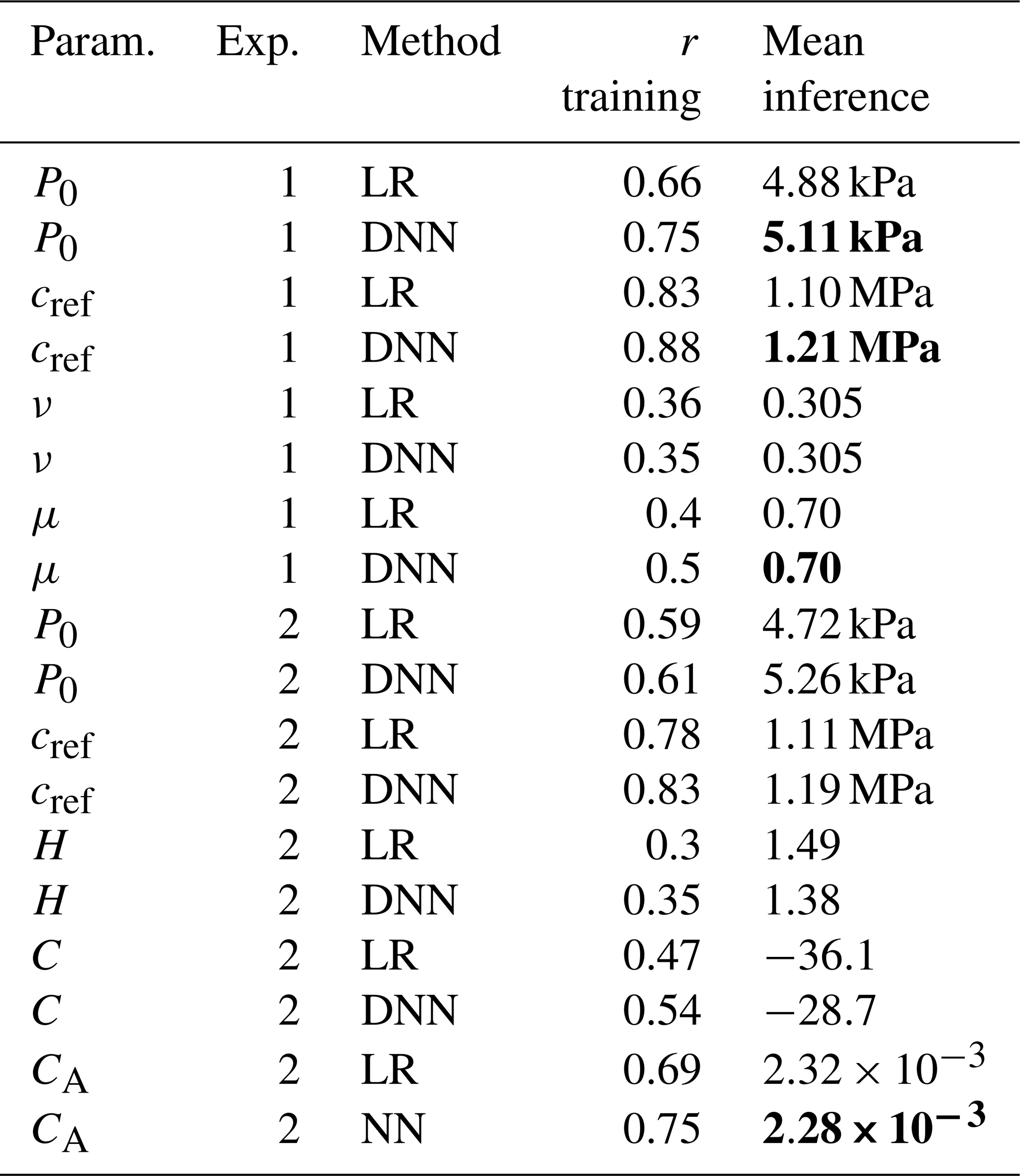
Figure 9 shows the DNN training results for the first (upper row) and second (lower row) experiments (see also Table 4). These scatterplots compare the actual and the predicted neXtSIM parameters from the test dataset from all 10 repetitions. In the first experiment, the DNN derives only the P₀ and c_ref with sufficient accuracy (correlations are 0.75 and 0.88, respectively). In the second experiment, the accuracy of the P₀ retrieval is somewhat lower (r=0.61), while the accuracy of the c_ref and C_A retrievals is high (correlations are 0.83 and 0.75, respectively). The DNN does not show any skill in retrieving ν or H parameters, and the accuracy of retrieving μ and C is somewhat higher for a short range of values. Still, overall, these four parameters cannot be derived with the machine learning approach. LR accuracy is lower (see Table 4), and the scatterplots are not shown.

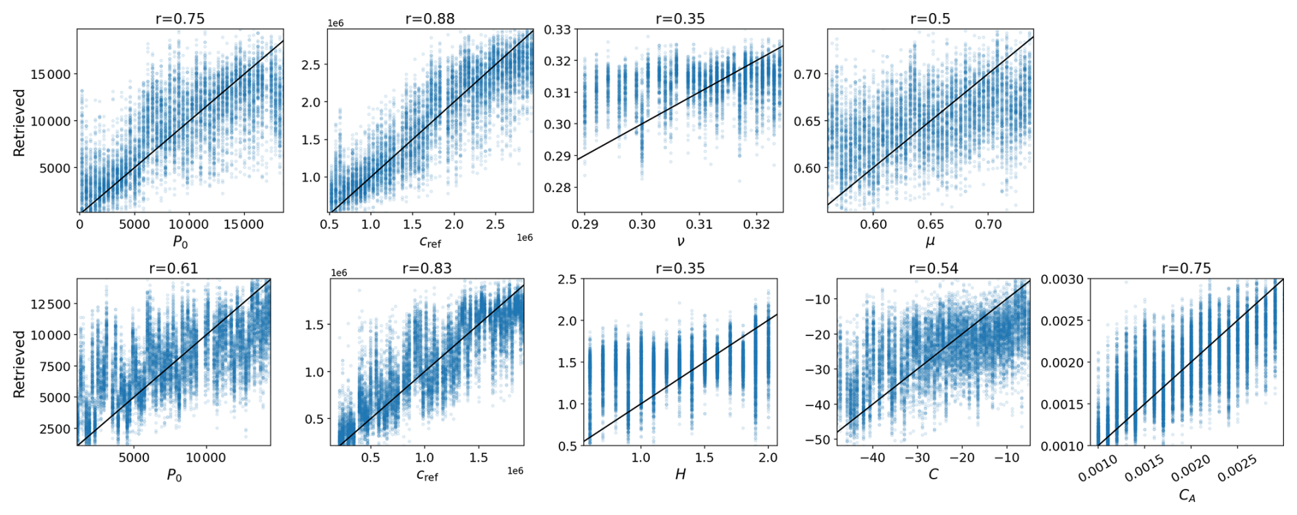
Figure 9 Comparison of the actual neXtSIM parameters (x axis) and the retrievals by the DNN. The upper row shows results from the first experiment, and the lower row shows the second experiment. The black lines show a 1:1 relation.

Figure 10 shows PDFs of parameters used for training (blue line) and derived from the RGPS data using DNN (orange line) and LR (green line) models in the two experiments mentioned above (upper and lower rows). In both experiments, PDFs of P₀ and c_ref parameters have a clear peak at ≈5000 kPa and ≈1.1 MPa, respectively. Notably, these peaks do not correspond to the centre of the distribution of the parameters used for training (blue line). We can observe similar behaviour for μ and C_A parameters, which also have relatively high retrieval accuracy for the testing data. For ν, H and C parameters, the situation is different – the accuracy of the retrievals for the testing data was low, and the retrievals from the RGPS data are centred on the distribution of training values.

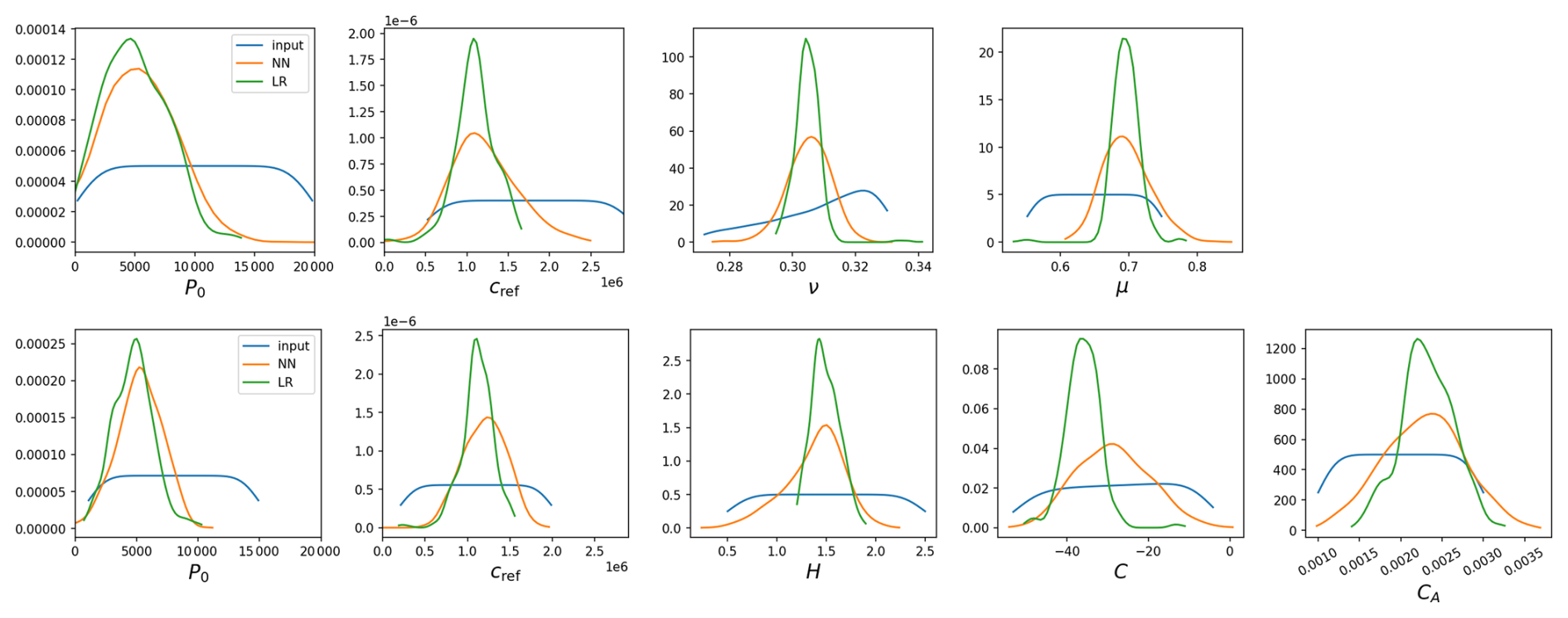
Figure 10 PDFs of parameters used for training (blue lines) and derived from RGPS descriptors using DNN (orange) and LR (green). The upper row shows the results from the first experiment, and the lower row shows results from the second experiment.

5.4 Optimal rheology parameters for neXtSIM

Since the training accuracy was high, the peaks of PDFs of RGPS-derived parameters are pronounced and have an offset from the centre of the input data distribution; we can conclude that the values of P₀, c_ref, μ and C_A parameters derived from RGPS can be used for optimal representation of the deformation patterns by neXtSIM. Table 4 lists the parameter values derived in different experiments and the accuracy of the model training. Note that the DNN always has higher accuracy than the LR model.

Table 4 Average values of neXtSIM parameters (Param.) derived from the RGPS. The optimal values are marked in bold.

We ran neXtSIM with the optimal parameter values, and Fig. 11 shows a comparison with RGPS for the three exact dates. We can see that the patterns of the divergence and shear fields are very similar for neXtSIM and RGPS concerning the density and orientation of LKFs, the magnitude of deformation, and (overall) the texture of the deformation field, thus confirming that the found parameters are indeed optimal.

We compared the PDFs of the deformation descriptors using the Kolmogorov–Smirnov (KS) test. The KS test is applied to the PDFs of deformation descriptors computed from neXtSIM and RGPS and is averaged over all usable descriptors. The average KS test is the lowest for the neXtSIM run with the optimal parameters (0.41) and is slightly lower than for the default parameters (0.49).

The simulated sea ice drift was validated against the RGPS drift by comparing the velocity vectors of each virtual buoy from RGPS data and the matching node on the neXtSIM mesh. The ice drift root-mean-square error for the run with optimal parameters is 0.04 m s⁻¹, slightly lower than for the run with the default parameters (0.05 m s⁻¹).

Sea ice thickness (SIT) from different runs was compared to the monthly average ice thickness from ICESat-1 in March 2007 (Zwally et al., 2014). SIT RMSE is the highest (≈1.3 m) for the runs with C_ref≈0.5 MPa, but no significant differences between the other runs were found (RMSE ≈1 m).

It is interesting to note similarities and differences between the parameters used by Ólason et al. (2022). We note that the values we get for ν, μ and H are very similar to those used by Ólason et al. (2022). This is to be expected for ν and μ, which are based on well-established values (see,  Weiss and Schulson, 2009; Mellor, 1986). Ólason et al. (2022) chose $H=\mathrm{3}/\mathrm{2}$ based on the modelling work of Hopkins (1998), but it is unclear whether this should be valid at the geophysical scale. The accuracy of our estimate for H is low, but it is reasonably close to $H=\mathrm{3}/\mathrm{2}$ and within the expected range of $H\in [\mathrm{1},\mathrm{2}]$.

In terms of the stress balance in the ice, C_A, P₀ and c_ref are the most important, as they determine the momentum transfer from atmosphere to ice, the resistance to ridging and the shear strength of the ice, respectively. Interestingly, our estimate of C_A is higher than the value used by Ólason et al. (2022); $\mathrm{2.28}\times {\mathrm{10}}^{-\mathrm{3}}$ vs. $\mathrm{2.0}\times {\mathrm{10}}^{-\mathrm{3}}$, resulting in more momentum transfer from the atmosphere to the ice. At the same time, both P₀ and c_ref are lower (5.11 vs. 10.0 kPa and 1.21 vs. 2.0 MPa, respectively). This results in an overall weaker ice cover compared to the parameters used by Ólason et al. (2022). It would, therefore, be reasonable to expect that our set of parameters would lead to an overestimate of the deformation, but this is not the case. This underlines the system's complexity and indicates that there may be multiple local minima in the parameter space, giving reasonable results. For such a system, using a systematic approach which samples the full parameter space – similar to what we propose here – is extremely beneficial.

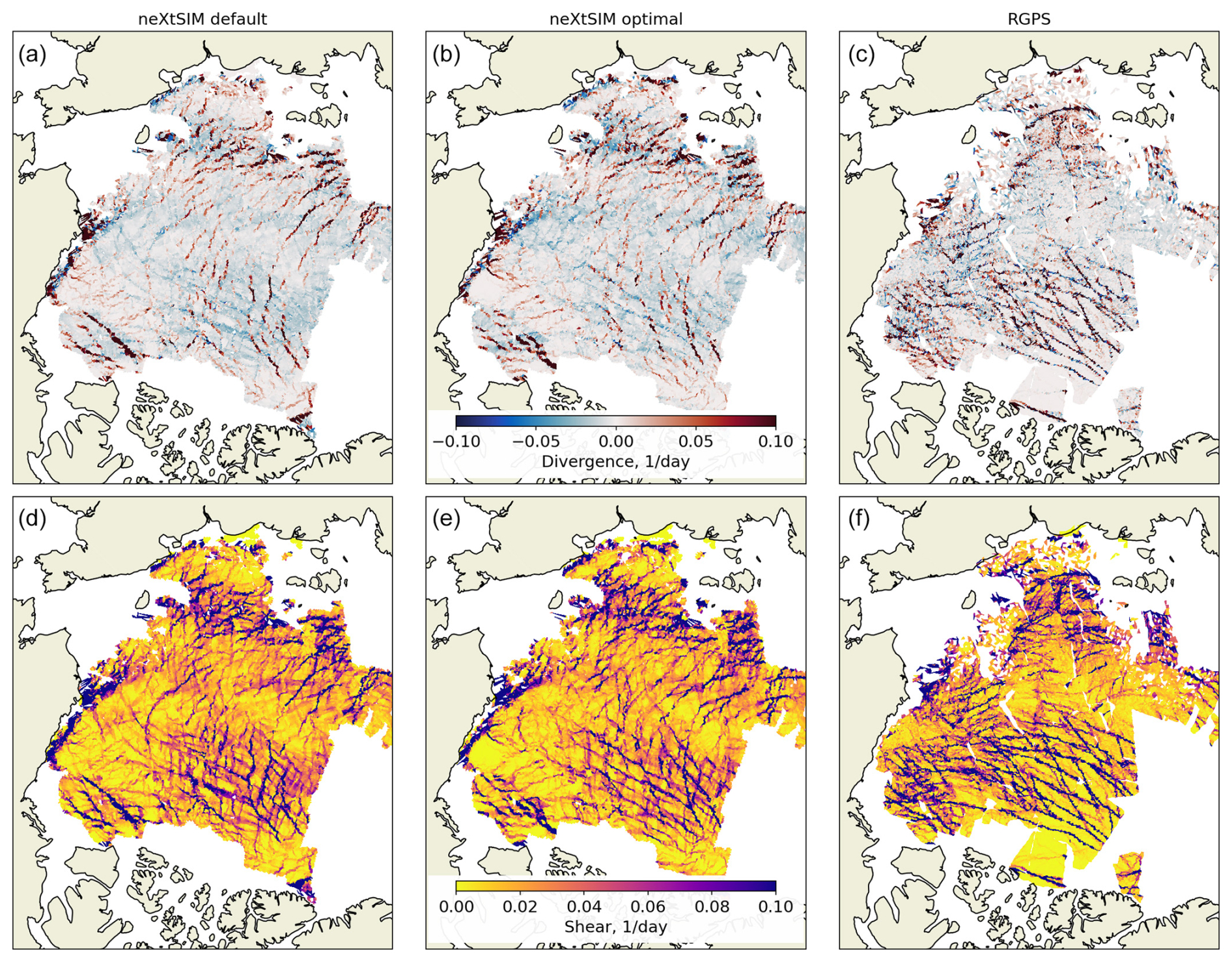
Figure 11 Maps of divergence and shear from the neXtSIM run with default parameters (a, d), optimal parameters (b, e) and from RGPS (c, f) for 3 February 2007.

5.5 Temporal variations of neXtSIM parameter values

The PDFs of parameters presented in Fig. 10 are derived from all RGPS descriptors computed in winter 2006–2007. However, we can also apply the ML model trained on neXtSIM data from winter 2006/07 to the RGPS data acquired since 1998. We applied the autoencoder described in Sects. 4.5 and 5.3 to the RGPS data from the earlier period to test if the trained ML model has sufficient generalisation skills. We could not detect any significant anomalies in these data. Since the encoder section of the autoencoder has the same architecture as the ML model used for inferring the rheology parameters, we can conclude that the ML model trained on data from winter 2006/07 is general enough to be applied to the earlier RGPS data. Figure 12 shows temporal variations of the derived optimal parameters on daily and interannual timescales. To create the latter plot, we computed the descriptors from the RGPS data for 1997–2008 and applied the DNN models trained on neXtSIM data from 2006–2007.

On daily timescales, the derived parameters show very high variability, reflecting frequent changes in the pattern of sea ice deformation due to varying atmospheric forcing. The DNN model from the first experiment is more sensitive to these variations and even produces unphysical negative values of P₀ during very high deformation at the beginning of February 2007. Despite substantial variability, the parameters are stable on the annual scale and do not show any significant trends.

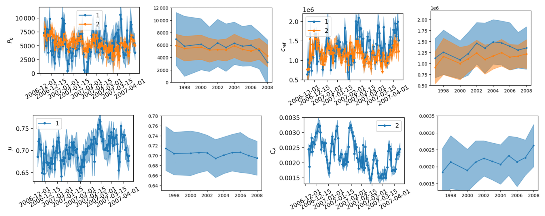
Figure 12 Time series of parameter values derived from RGPS for 1 year (left column) and several years (right column). Colour denotes the experiment, and the shaded area shows the standard deviation of samples produced by 10 neural networks for the daily values (left column) or the samples collected from the entire year (right column).

On the interannual scale, the parameters tend to change; P₀ and μ slightly decrease, while c_ref and A_C gradually increase. A gradual change in the observed pattern of sea ice deformation can explain this observation. In the 1990s, thicker ice had sparser and more pronounced LKFs (see Fig. 4: high P₀ and low c_ref maps). As ice became thinner, more background deformation appeared, LKFs became denser and the magnitude of deformation in LKFs slightly decreased (see Fig. 4: low P₀ and high c_ref maps). The impact of internal friction angle or air drag is not shown in Fig. 4, but the mechanisms are similar: higher Mohr–Coulomb slope allows the ice to resist breakup longer and creates larger floes (mimicking the earlier, thicker ice situation); a low air coefficient decreases ice drift and, consequently, ice deformation, which again corresponds to an earlier period of RGPS observations.

After the first experiments, we observed the interannual trends in the P₀ and c_ref parameters (see Fig. 12). This leads us to conclude that the weak dependence of these rheology parameters on ice thickness (and potentially concentration) indicates that the parameterisation of P_max (see Eq. 2) requires optimised tuning of H and C parameters. That was the motivation to run the second experiment and to retrieve values of H, C and C_A. Unfortunately, as Table 4 shows, the accuracy of ML models for these parameters is not sufficiently high, and we cannot derive their optimal values. Nevertheless, accounting for these parameters in the second experiment allowed us to train ML models that show fewer diurnal variations and are more stable on interannual timescales. Moreover, despite low accuracy, the ML models predict lower values of H (1.38) and C (−28.7) than the default ones. Dedicated experiments are needed to tune these parameters further.

6 Conclusions

We developed a new set of metrics for characterising the patterns in the sea ice deformation fields. These metrics are sensitive to the parameters of a sea ice model rheology and can be used to compare simulated and observed ice deformation for model evaluation or parameter tuning.

We developed a new method for tuning model parameters using machine learning. In our process, we train an ML model using simulated data and apply it to observations. In our case, the inputs to the ML model are the descriptors of sea ice deformation, and the targets are the sea ice rheology parameters. We tested a linear regression (LR) and a deep neural network (DNN) as ML models, and DNN always showed higher accuracy. This method can be applied to tune the parameters of any other model.

Using the new set of metrics and the new ML-based method, we found values of four BBM rheology parameters that were poorly constrained previously: scaling parameter for compressive strength (P₀≈5.1 kPa), cohesion at the reference scale (c_ref≈1.2 MPa), internal friction angle tangent (μ≈0.7) and ice–atmosphere drag coefficient (C_A≈0.00228).

Our experiments cover a wide range of weather and sea ice conditions: from thin young ice in the eastern Arctic to thick multiyear ice (MYI) near the Canadian Arctic Archipelago, from the beginning to the end of the freezing period and from calm days to winter storms. Presumably, the ML model trained on such heterogeneous data is general enough to be applied in regions with similar ice conditions, e.g. Laptev, Kara, Barents, and Lincoln seas in the Arctic or Weddell and Ross seas in the Antarctic. Applying neXtSIM in the Antarctic shows that the model reproduces the seasonal cycle of sea ice extent and that the BBM rheology simulates the sea ice drift with higher accuracy (Santana et al., 2024). In other regions (e.g. the marginal ice zone), where the conditions are quite different, the sea ice concentration is lower; the ice elasticity drops substantially (see Eq. 4); and the rheology is no longer sensitive to c_ref, P, or other parameters.

The tuned parameters exhibit weak interannual drift related to changes in sea ice thickness and corresponding changes in ice deformation patterns. Improving the dependence on thickness and concentration in the BBM rheology or tuning the corresponding parameters may reduce the drift and make the rheology completely independent of the ice thickness influence. Recent observations of ice drift and deformation obtained from Sentinel-1 SAR data processing are recommended for tuning the rheology to reflect the current situation and provide higher-accuracy forecasts.

Other parameters in our experiments (exponent of compression factor, Poisson's ratio, compaction parameter) did not impact the pattern of sea ice deformation, or the influence of other parameters masked their impact. Therefore, their values could not be derived using our method. Dedicated experiments are required to study the sensitivity of the proposed metrics to these parameters and to tune their values.

Appendix A: Additional figures

Figure A1 presents a scheme of the Bingham–Maxwell rheology, where a spring is connected in series with a block, where a dashpot and a friction element are connected in parallel.

Figure A2.A shows examples of RGPS trajectories spanning 150–180 d, and Fig. A2b shows positions of virtual buoys detected on SAR images acquired between 1 and 5 January 2007. Points are coloured by the time of image acquisition. Panel (c) in Fig. A2 shows the shear component of deformation computed from the drift of buoys shown on panel (b). The figure illustrates how heterogeneous the RGPS Lagrangian ice motion data are in space and time.

Figure A3 shows a colocation of a neXtSIM mesh (shown in black) and a triangulated subset from the RGPS dataset (shown in red). The RGPS subset is created by selecting starting and ending virtual buoy positions belonging to the same RADARSAT-1 images separated by 3 d. All nodes on the neXtSIM mesh within 10 km from the RGPS subset are selected (blue) and used for the computation of deformation.

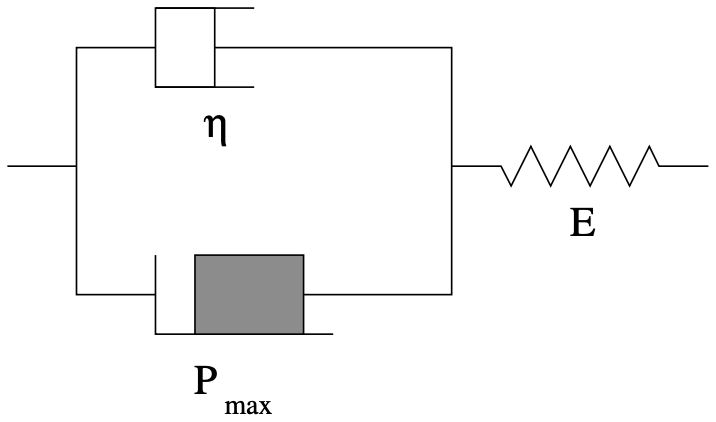
Figure A1 A schematic of the Bingham–Maxwell constitutive model showing a dashpot and a friction element connected in parallel, with both connected to a spring in series. The figure is adapted from Ólason et al. (2022).

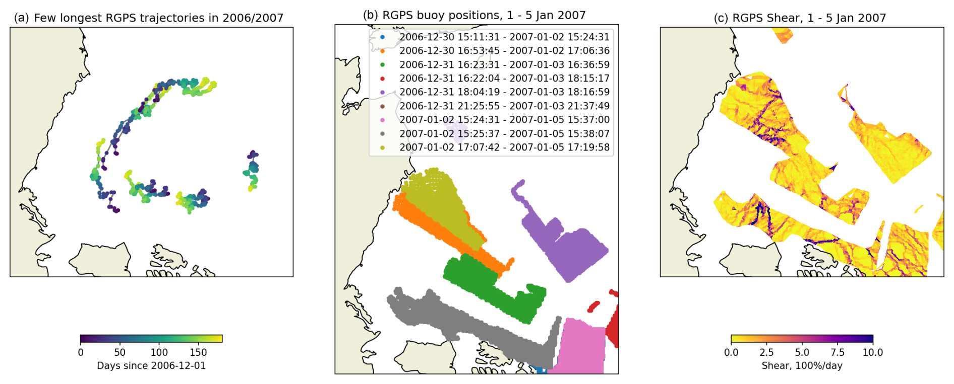
Figure A2 (a) Example trajectories of virtual buoys detected on RADARSAT-1 data by the RGPS between 1 December 2006 and 15 May 2007. (b) Position of virtual buoys on SAR images acquired between 1 and 5 January 2007. Points are coloured by the starting and ending image acquisition times, as shown in the legend. (c) Shear computed from the RADARSAT-1 image pairs shown on (b).

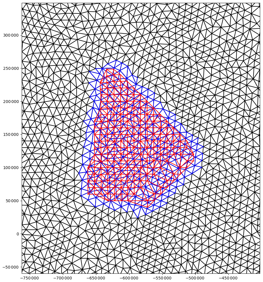
Figure A3 Illustration of the RGPS and neXtSIM mesh colocation. The neXtSIM mesh from one snapshot is shown in black. The RGPS mesh created by triangulation of virtual drifters detected on a pair of RADARSAT-2 images is shown in red. The neXtSIM mesh subsampled from the original mesh for colocation with the RGPS mesh is shown in blue.

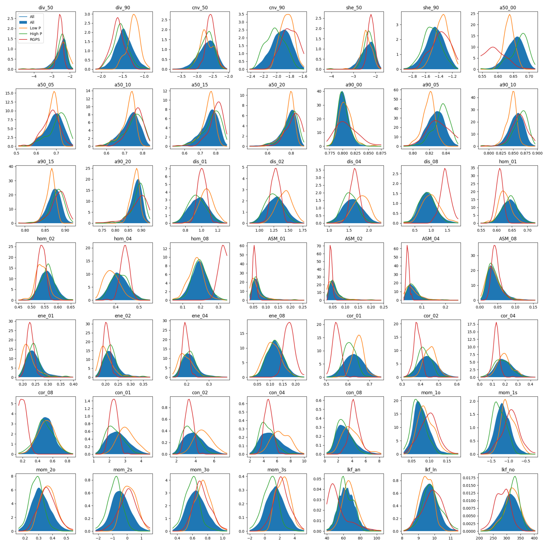
Figure A4 PDFs of all deformation descriptors for RGPS (red), all neXtSIM runs (blue), and runs with lowest (orange) or highest values of P₀.