Developing an eco-physiological process-based model of soybean growth and yield (MATCRO-Soy v.1): model calibration and evaluation

MATCRO-Soy is an eco-physiological process-based crop model for soybean (Glycine max L. (Merr.)). It was developed by modifying the parameters of MATCRO-Rice, which integrates crop growth processes with a land surface model. The original model was modified using data from the literature and field experiments conducted in countries around the world. The reliability of the model was extensively validated by comparing the simulated yields with observed yields at global, national, and grid-cell levels. Moderate correlations were detected between the yields predicted by MATCRO-Soy and yield data in the Food and Agriculture Organization's FAOSTAT database, with correlation coefficients of 0.81 (p<0.001) for the global average yield and 0.45 (p<0.01) for the global average detrended yield over a 34 year period (1981–2014). Furthermore, validation at the grid-cell level revealed a statistically significant correlation between the MATCRO-Soy simulated yield and the observed yield in 66 % of the grid cells in the global yield map. These results highlight the model's ability to reproduce soybean yield under different environmental conditions, integrating soil water availability and nitrogen fertilizer levels. The MATCRO-Soy model may enhance our understanding of crop physiology, especially crop responses to climate change. Its application may support efforts to reduce uncertainty in projections of the effects of climate change on soybean crops.

1 Introduction

Crop growth models are widely used for estimating yield, optimizing agricultural management practices, evaluating the effects of climate change, and informing decision-making about food security strategies (Adeboye et al., 2021; Cuddington et al., 2013; Hoogenboom, 2000). Given the significant impact of weather variability on global crop yields (Müller et al., 2017; Ray et al., 2015), process-based models can predict the effects of long-term climate change on productivity by accounting for the effects of key climatic factors on physiological processes that are represented in the model (Boote et al., 2013; Cuddington et al., 2013; Fodor et al., 2017; Jones et al., 2017; Marin et al., 2014; Stöckle and Kemanian, 2020). Process-based models explicitly incorporate the crucial eco-physiological processes of photosynthesis and stomatal conductance. Thus, the predictive ability of these models is improved under varying climate scenarios compared with that of models that focus on the empirical relationship between absorbed radiation and assimilation through radiation use efficiency (Jin et al., 2018). Hence, crop models are useful for capturing the complexity of soil–crop–climate interactions for ensuring food security, optimizing yields, promoting sustainability, and planning adaptation strategies (García-Tejero et al., 2011). Global-scale simulations are crucial for enhancing these efforts because they reflect the interactions between physiological processes and environmental factors, thereby supporting adaptive management practices and strengthening agricultural resilience.

The Agricultural Model Intercomparison and Improvement Project (AgMIP) has examined the performance of global gridded crop models (GGCMs) in simulating the potential impact of climate change on crop yields (Müller et al., 2017). The AgMIP has demonstrated that the simulated impacts of environmental factors on crop yields using a GGCM generally align with measured values, and that a model ensemble reduces uncertainty (Elliott et al., 2015). However, yield changes under future climate change scenarios show inconsistent results and greater variability in soybean (Glycine max L. (Merr.)) than in other crops, because of model discrepancies (Jägermeyr et al., 2021). Despite being a major crop, soybean has been studied less extensively than other crops in terms of its response to changing environments (Ruane et al., 2017; Kothari et al., 2022). Therefore, the development of a new soybean model is needed to reduce uncertainties in climate change impact assessments.

It is important to use diverse types of crop models and ensure model diversity to understand the uncertainties of simulations, because relying on a single model can lead to biased results. To our knowledge, there are only five process-based models for global-scale soybean yield estimation with leaf-level photosynthesis and stomatal conductance parameters; namely LPJ-GUESS (Ma et al., 2022), LPJmL (Wirth et al., 2024), ORCHIDEE-crop (Wu et al., 2016), PRYSBI2 (Sakurai et al., 2014), and JULES (Leung et al., 2020). Simulations for soybean using process-based models are relatively uncommon. Thus, further development and validation of process-based models that incorporate leaf-level photosynthesis and stomatal conductance parameters are essential.

MATCRO-Rice (Masutomi et al., 2016a, b) is an ecosystem process-based model for crops embedded into the land surface model of Minimal Advanced Treatments of Surface Interaction and Runoff (MATSIRO; Takata et al., 2003). The crop growth model is further explained in Sect. 2. MATCRO-Rice uses state variables to exchange information (e.g., temperature, soil moisture, transpiration, leaf area index, and photosynthesis rate) between the land surface model and crop growth model. The MATCRO-Rice model incorporates mechanisms related to photosynthesis and stomatal conductance to assess the impact of greenhouse gases on carbon and water fluxes on crop yield. Masutomi et al. (2019) described the implementation of ozone effects as one of these mechanisms, highlighting the model's capability to account for environmental stressors. Furthermore, MATCRO-Rice has been applied at the regional scale, and it has been used to measure climate impacts, which are important for developing adaptation strategies (Kinose et al., 2020; Masutomi, et al., 2016b).

Here, we developed a new process-based model for soybean, MATCRO-Soy v.1, which incorporates diverse biological processes and environmental interactions that drive plant growth and adaptation to changing conditions. Adapted from MATCRO-Rice, the new model was applied to soybean by parameterizing key processes using experimental data and findings from the literature. The current version of MATCRO-Soy (v.1) was evaluated in a global-scale simulation, following a calibration process that considered essential photosynthesis mechanisms. This paper presents the model description in Sect. 2, the calibration process in Sect. 3, and the model evaluation in Sects. 4 and 5.

2 Model description

MATCRO-Soy is based on MATCRO-Rice, a process-based model for rice growth and yield. Here, the MATCRO-Rice model has been modified for use in soybean. MATCRO-Rice is a combined land surface and crop growth model used to explore the land–atmosphere interaction in rice fields. Unlike MATCRO-Rice v.1, MATCRO-Soy focuses on yield simulation and omits the calculation of sensible and latent heat fluxes in the energy balance to reduce computational complexity while maintaining accuracy in simulating soybean growth and yield.

2.1 Overview of MATCRO-Soy

MATCRO-Soy includes three main modules: phenology, photosynthesis, and carbon partitioning (Fig. 1). The phenology module simulates crop phenological development over time based on heat unit accumulation. The module directs the progression of carbon assimilation and partitioning by monitoring plant developmental stages from sowing to harvest. The phenology module simulates developmental stages based on the developmental rate from sowing to harvest. The developmental stage influences key processes such as glucose production and allocation across plant organs. The photosynthesis module initially estimates gross primary production (GPP) and respiration at the leaf level using the Farquhar model (Farquhar et al., 1980), and then extends the estimation of net primary production (NPP) to the canopy level, following the concept introduced by de Pury and Farquhar (1997). It considers the electron-transport-limited rate of photosynthesis, Rubisco-limited photosynthesis, and leaf respiration to estimate NPP at the leaf level.

Figure 1 Flowchart diagram of soybean yield simulation by the MATCRO-Soy model.

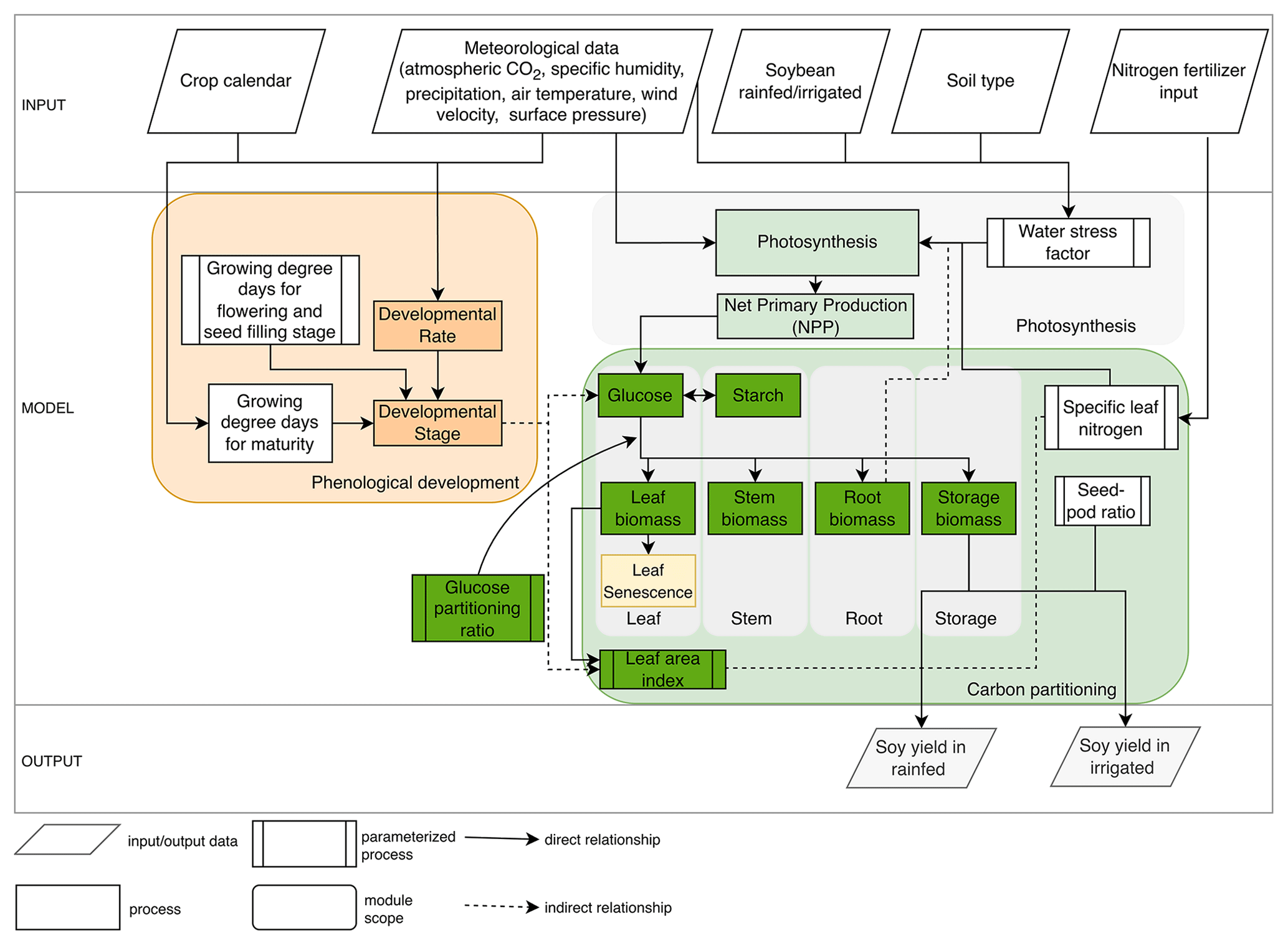
The photosynthesis and carbon partitioning modules are closely linked, because carbon assimilated from photosynthesis is subsequently allocated to different plant organs. The NPP is stored in glucose and starch reserves. The carbon partitioning module distributes glucose to different organs (i.e., leaf, stem, root, and storage organ) using a method derived from the school of de Wit, which simulates biosynthetic processes (de Vries et al., 1989). It also accounts for leaf senescence, which influences nutrient cycling, crop productivity, and the leaf area index, thereby affecting canopy photosynthesis. Leaf senescence is simulated as a function of crop developmental stage, as defined by the phenology module. MATCRO incorporates the amount of nitrogen per leaf area (specific leaf nitrogen, SLN) as a key determinant of photosynthetic capacity. Root depth can indirectly affect photosynthesis because it influences the plant's ability to access water and nutrients from soil layers, further influencing plant growth within the model framework.

The input data consisted of environmental variables obtained from meteorological forcings, soil type classifications, nitrogen fertilizer applications, and agricultural management practices such as irrigation and seed sowing. These inputs were crucial for setting the initial conditions and boundary parameters for the simulations. The output of MATCRO is crop yield (kg ha⁻¹) estimated for both irrigated and rainfed conditions on the basis of soil–crop interactions. First, we processed the parameterized growing degree days to maturity using crop calendar data to estimate the harvest time in the phenology module (see Sect. 2.2). The photosynthesis module includes limiting factors such as nitrogen fertilization and water stress, as detailed in Sect. 2.3. Then, crop growth is calculated based on developmental stage (Sect. 2.4). We conducted a parameterization process including phenological development, carbon partitioning, and photosynthesis limited by water stress and nitrogen uptake. The crop yield was estimated using the parameterized seed:pod ratio (see Sect. 2.5). The adjusted parameters in MATCRO-Soy are described in Sect. 2.6, where the key dynamic variables were parameterized over time to ensure a reliable estimate of carbon assimilation in soybean. This comprehensive approach allows MATCRO to account for the complex interactions among environmental conditions, crop physiology, and management practices, providing a robust framework for predicting crop yields and assessing agricultural productivity.

2.2 Crop phenological development

Phenological development refers to the timing of developmental events in response to environmental inputs. MATCRO calculates crop developmental stage (DVS) using an index ranging from 0–1, where DVS=0 is the sowing time and DVS=1 is maturity. This index is based on the integral of the temperature required to exceed the phenological changes. The module uses a formulation based on Bouman et al. (2001) as outlined in Eqs. (1)–(4) as follows:

$$\begin{array}{}\text{(1)}& {\displaystyle }& {\displaystyle }{\text{DVS}}_{\mathrm{t}}={\displaystyle \frac{{\text{GDD}}_{\mathrm{t}}}{{\text{GDD}}_{\mathrm{m}}}}\text{(2)}& {\displaystyle }& {\displaystyle }{\text{GDD}}_{\mathrm{t}}=\underset{\mathrm{0}}{\overset{t}{\int }}\text{DVR}\mathrm{d}{t}^{\prime }\text{(3)}& {\displaystyle }& {\displaystyle }{\text{GDD}}_{\mathrm{m}}=\underset{\mathrm{0}}{\overset{m}{\int }}\text{DVR}\mathrm{d}{t}^{\prime }\text{(4)}& {\displaystyle }& {\displaystyle }{\text{DVR}}_{\mathrm{t}}=\left\{\begin{array}{ll}\mathrm{0},& T_{\mathrm{t}}<T_{\mathrm{b}}\mathrm{|}{T}_{\mathrm{t}}>T_{\mathrm{h}}\\ T_{\mathrm{t}}-T_{\mathrm{b}},& T_{\mathrm{b}}<T_{\mathrm{t}}<T_{\mathrm{o}}\\ {\displaystyle \frac{(T_{\mathrm{o}}-T_{\mathrm{b}})(T_{\mathrm{h}}-T_{\mathrm{t}})}{(T_{\mathrm{h}}-T_{\mathrm{o}})}},& T_{\mathrm{o}}<T_{\mathrm{t}}<T_{\mathrm{h}}\end{array}\right.\end{array}$$

where GDD_t and GDD_m indicate the growing degree days (°C days) used to estimate the development of plants during the growing season at time t and at maturity (m), respectively; DVR represents the developmental rate at t; and T_t represents the temperature at t. The parameters T_b, T_o, and T_h (°C) are crop-specific and represent the base, optimum, and highest temperatures for crop development, respectively.

The impact of temperature on phenological stage can differ among crop stages, as Boote et al. (1998) observed that cardinal temperatures (T_b, T_h, T_o) may differ between vegetative and reproductive stages. We followed de Vries et al. (1989) for cardinal temperatures during the growing season. This study parameterized the developmental stages as flowering (DVS_f), seed-filling (DVS_s), and maturation (DVS_m) on the basis of mean values calculated from the available observations for each stage (listed in Table 2). Calculations for each stage were based only on experiments where corresponding data were available. MATCRO uses these DVS parameters to define the period of leaf dry weight loss due to leaf senescence and the remobilization of starch reserves from the stem (Masutomi et al., 2016a). It was assumed that the corresponding phenological times in soybean are the middle of the flowering stage and the seed-filling stage, because leaf loss starts within those periods.

2.3 Carbon assimilation process

In the photosynthesis module of MATCRO-Soy, carbon assimilation is based on canopy photosynthesis, which is estimated from leaf-level photosynthesis calculated in sunlit and shaded conditions (Dai et al., 2004). The calculation includes the stomatal conductance response to relative humidity (Collatz et al., 1991). The net carbon assimilation (A_n) in MATCRO is calculated using the Farquhar model as further described in Masutomi et al. (2016a), expressed in Eq. (5) as given as

$$\begin{array}{}\text{(5)}& A_{\mathrm{n}}=f(\text{PAR},{\text{CO}}_{\text{2leaf}},V_{max},P_{\mathrm{a}},\text{RH},T_{\text{leaf}},f_{\mathrm{w}},{\text{BB}}_{\mathrm{a}},{\text{BB}}_{\mathrm{b}})\end{array}$$

where A_n ($\mathrm{mol}\left({\mathrm{CO}}_{\mathrm{2}}\right){\mathrm{m}}^{-\mathrm{2}}{\mathrm{s}}^{-\mathrm{1}}$) represents net carbon assimilation contributing to NPP for biomass growth. It is a function of the intensity of absorbed photosynthetic active radiation (PAR, in $\mathrm{mol}\left(\mathrm{photon}\right){\mathrm{m}}^{-\mathrm{2}}{\mathrm{s}}^{-\mathrm{1}}$), the CO₂ concentration in the substomatal chamber (CO_2 leaf, in Pa(CO₂) Pa(Air)⁻¹), maximum Rubisco capacity per unit leaf area (V_max, in $\mathrm{mol}\left({\mathrm{CO}}_{\mathrm{2}}\right){\mathrm{m}}^{-\mathrm{2}}{\mathrm{s}}^{-\mathrm{1}}$), air pressure (P_a, in Pa), relative humidity (RH), leaf temperature (T_leaf, in K), water stress factor (f_w, dimensionless), the slope (BB_a, in $\mathrm{mol}\left({\mathrm{H}}_{\mathrm{2}}\mathrm{O}\right){\mathrm{m}}^{-\mathrm{2}}{\mathrm{s}}^{-\mathrm{1}}$) and intercept (BB_b, in $\mathrm{mol}\left({\mathrm{H}}_{\mathrm{2}}\mathrm{O}\right){\mathrm{m}}^{-\mathrm{2}}{\mathrm{s}}^{-\mathrm{1}}$) of the Ball–Berry model of the relationship between crop assimilation and stomatal conductance per unit leaf area, relative humidity at the leaf surface, and ambient CO₂ concentration (Ball, 1988). The leaf temperature is assumed to be the same as the air temperature to simplify the calculation.

Rubisco activity is a key variable used to assess the rate of carbon entry into the photosynthetic pathway, because Rubisco catalyzes the crucial initial step of RuBP (ribulose-1,5-bisphosphate) carboxylation in photosynthetic carbon assimilation in C₃ plants (Sage, 2002; Xu et al., 2022). In MATCRO, V_max in Eq. (5) is calculated as follows:

$$\begin{array}{}\text{(6)}& {\displaystyle }& {\displaystyle }{V}_{max}=V_{\text{mc}}{f}_{\mathrm{w}}\text{(7)}& {\displaystyle }& {\displaystyle }{V}_{\text{mc}}={\stackrel{\mathrm{‾}}{V}}_{\text{mc}}\exp (c-\mathrm{\Delta }H/R{T}_{\text{leaf}})\text{(8)}& {\displaystyle }& {\displaystyle }{\stackrel{\mathrm{‾}}{V}}_{\text{mc}}={\displaystyle \frac{{\int }_{\mathrm{0}}^{\text{LAI}}{V}_{\text{cmax}}\left(\text{LAI}\right)\mathrm{d}\text{LAI}}{\text{LAI}}}\end{array}$$

where V_max and V_mc are, respectively, the maximum Rubisco capacity per unit leaf area with and without the water stress factor (f_w); V_mc is determined with a generic temperature response as described by Bernacchi et al. (2001); c and ΔH represent a scaling constant (c=26.35) and activation energy ($\mathrm{\Delta }H=\mathrm{65.33}\mathrm{kJ}{\mathrm{mol}}^{-\mathrm{1}}$) of Rubisco's activity response to temperature changes; R is the molar gas constant in kJ mol⁻¹; ${\stackrel{\mathrm{‾}}{V}}_{\text{mc}}$ is the maximum Rubisco capacity averaged over the canopy; and V_cmax(LAI) denotes the vertical distribution of the maximum Rubisco capacity through the canopy, as determined by the vertical nitrogen distribution (see Eqs. 14 and 15). The water stress factor, f_w, is determined based on the root distribution function (f_r(i)) multiplied by the water stress function at each soil layer (f_wstress,t(i)). The results are then summed across five soil layers (depths of 0.05, 0.25, 1, 2, and 4 m below the ground surface), as given in Eqs. (9)–(13) as follows:

$$\begin{array}{}\text{(9)}& {\displaystyle }& {\displaystyle }{f}_{\mathrm{w}}=\sum _{i=\mathrm{1}}^{\mathrm{5}}{f}_{\mathrm{r}}\left(i\right)f_{\text{wstress},t}\left(i\right)\text{(10)}& {\displaystyle }& {\displaystyle }{f}_{\mathrm{r}}\left(i\right)=\left({\displaystyle \frac{\mathrm{3}}{\mathrm{2}}}\right){\displaystyle \frac{\left(z_{\mathrm{r}}^{\mathrm{2}}-i^{\mathrm{2}}\right)}{z_{\mathrm{r}}^{\mathrm{3}}}}\text{(11)}& {\displaystyle }& {\displaystyle }{z}_{\mathrm{r}}=min\left\{z_{\text{rootmax}},r_{\text{root}}(t-t_{\mathrm{e}})\right\}\end{array}$$

where f_r(i) is the distribution of roots in soil layer i (with value of 1–5). Root depth (z_r, in m) is calculated based on the root growth rate (r_root, m d⁻¹) in timestep t (day) after the time of emergence (t_e, in d), and is limited by the maximum root depth (z_rootmax, in m). t_e is assumed to be in the early developmental stage (0.012 of the growing period). The function f_wstress,t represents a simplified version of the relationship between the soybean transpiration ratio and transpirable soil water devised by Ray and Sinclair (1998), given in Eq. (12).

$$\begin{array}{}\text{(12)}& f_{\text{wstress},t}\left(i\right)=\left\{\begin{array}{ll}\frac{\mathrm{1}}{\mathrm{0.5}}\text{FAW}\left(i\right),& \text{if FAW}\left(i\right)\le \mathrm{0.5}\\ \mathrm{1},& \text{if FAW}\left(i\right)>\mathrm{0.5}\end{array}\right.\end{array}$$

The value of the water stress function at timestep t (f_wstress,t) depends on soil water availability at soil layer i (FAW_i), which is the estimated soil water content based on the water flux between the soil layers during crop growth calculated by

$$\begin{array}{}\text{(13)}& \text{FAW}\left(i\right)={\displaystyle \frac{\text{WSL}\left(i\right)-{\text{WSL}}_{\text{wilt}}}{{\text{WSL}}_{\text{FC}}-{\text{WSL}}_{\text{wilt}}}}\end{array}$$

where WSL(i), WSL_wilt, and WSL_FC represent the water levels in the soil layer i, at wilting point, and at field capacity, respectively. A value of f_wstress equal to 1 indicates no water stress because the fraction of available soil water is adequate for crop growth.

V_cmax(LAI) is the reference value for maximum Rubisco activity within the canopy ($\mathrm{mol}\left({\mathrm{CO}}_{\mathrm{2}}\right){\mathrm{m}}^{-\mathrm{2}}{\mathrm{s}}^{-\mathrm{1}}$) at leaf area index (LAI, in m² m⁻²) depth, limited by the exponential value of vertical distribution of leaf nitrogen (K_n), and the reference value for maximum Rubisco activity at the top of canopy (V_ctop, in $\mathrm{mol}\left({\mathrm{CO}}_{\mathrm{2}}\right){\mathrm{m}}^{-\mathrm{2}}{\mathrm{s}}^{-\mathrm{1}}$), calculated as follows:

$$\begin{array}{}\text{(14)}& {\displaystyle }& {\displaystyle }{V}_{\text{cmax}}\left(\text{LAI}\right)=V_{\text{ctop}}\exp (-K_{\mathrm{n}}\text{LAI})\text{(15)}& {\displaystyle }& {\displaystyle }{V}_{\text{ctop}}=max(a{\text{SLN}}^{\mathrm{2}}+b\text{SLN}+c,V_{\text{ctopmax}})\end{array}$$

For soybean, the V_ctop photosynthetic rate limited by the SLN is based on the relationship between Rubisco activity and leaf nitrogen content, as determined from experiments on soybean at the reproductive stage, summarized by Ainsworth et al. (2014), and for soybean at the reproductive stage, summarized by Qiang et al. (2022). This relationship is empirically represented by a polynomial quadratic equation limited by the maximum value of Rubisco activity at the top canopy (V_ctopmax in $\mathrm{mol}\left({\mathrm{CO}}_{\mathrm{2}}\right){\mathrm{m}}^{-\mathrm{2}}{\mathrm{s}}^{-\mathrm{1}}$). a, b, c are the quadratic coefficient, linear coefficient, and constant, respectively, from the relationship between the two variables based on data digitized using WebPlotDigitizer (Rohatgi, 2023).

MATCRO considers nitrogen fertilization input denoted as N_fert (unit: kg(N) ha⁻¹). This influences the amount of SLN (g(N) m⁻²), particularly under conditions of limited nitrogen availability (Cafaro La Menza et al., 2023; Thies et al., 1995). The SLN is determined by nitrogen supply (including biological nitrogen fixation, soil mineral nitrogen, and nitrogen fertilizer) and by plant demand. In MATCRO-Soy, the changes in SLN over the growing period are represented by a function derived from Cafaro La Menza et al. (2023), who observed SLN under wide range of low- and high-nitrogen fertilization conditions (see Fig. S1 in the Supplement). This function adjusts the SLN value during the crop growth period, and higher nitrogen fertilization levels result in a higher leaf nitrogen content. In the absence of empirical data for initial growth stages, the model assumes a gradual increase in nitrogen content. The simulated SLN under different nitrogen fertilization treatments is defined by

$$\begin{array}{}\text{(16)}& {\displaystyle }& {\displaystyle }\text{SLN}=\left\{\begin{array}{l}{\text{SLN}}_{Y\mathrm{0}}+{\displaystyle \frac{({\text{SLN}}_{Y\mathrm{1}}-{\text{SLN}}_{Y\mathrm{0}})(\text{DVS}-{\text{SLN}}_{X\mathrm{1}})}{{\text{SLN}}_{X\mathrm{1}}}},\\ \text{if DVS}<{\text{SLN}}_{X\mathrm{1}}\\ {\text{SLN}}_{Y\mathrm{2}}+{\displaystyle \frac{({\text{SLN}}_{Y\mathrm{2}}-{\text{SLN}}_{Y\mathrm{1}})(\text{DVS}-{\text{DVS}}_{\mathrm{f}})}{({\text{DVS}}_{\mathrm{f}}-{\text{SLN}}_{X\mathrm{1}})}},\\ {\text{if SLN}}_{X\mathrm{1}}\le \text{DVS}<{\text{DVS}}_{\mathrm{f}}\\ Y+{\displaystyle \frac{(Y-{\text{SLN}}_{Y\mathrm{2}})(\text{DVS}-{\text{DVS}}_{\mathrm{s}})}{({\text{DVS}}_{\mathrm{s}}-{\text{DVS}}_{\mathrm{f}})}},\\ {\text{if DVS}}_{\mathrm{f}}\le \text{DVS}<{\text{DVS}}_{\mathrm{s}}\\ {\text{SLN}}_{Y\mathrm{0}}+{\displaystyle \frac{({\text{SLN}}_{Y\mathrm{0}}-Y)(\text{DVS}-{\text{DVS}}_{\mathrm{m}})}{({\text{DVS}}_{\mathrm{m}}-{\text{DVS}}_{\mathrm{s}})}},\\ {\text{if DVS}}_{\mathrm{s}}\le \text{DVS}\le {\text{DVS}}_{\mathrm{m}}\end{array}\right.\text{(17)}& {\displaystyle }& {\displaystyle }Y={\text{SLN}}_{Y\mathrm{3},\mathrm{l}}+{\displaystyle \frac{{\text{SLN}}_{Y\mathrm{3},\mathrm{h}}-{\text{SLN}}_{Y\mathrm{3},\mathrm{l}}}{N_{\text{fert,high}}}}\times N_{\text{fert}}\end{array}$$

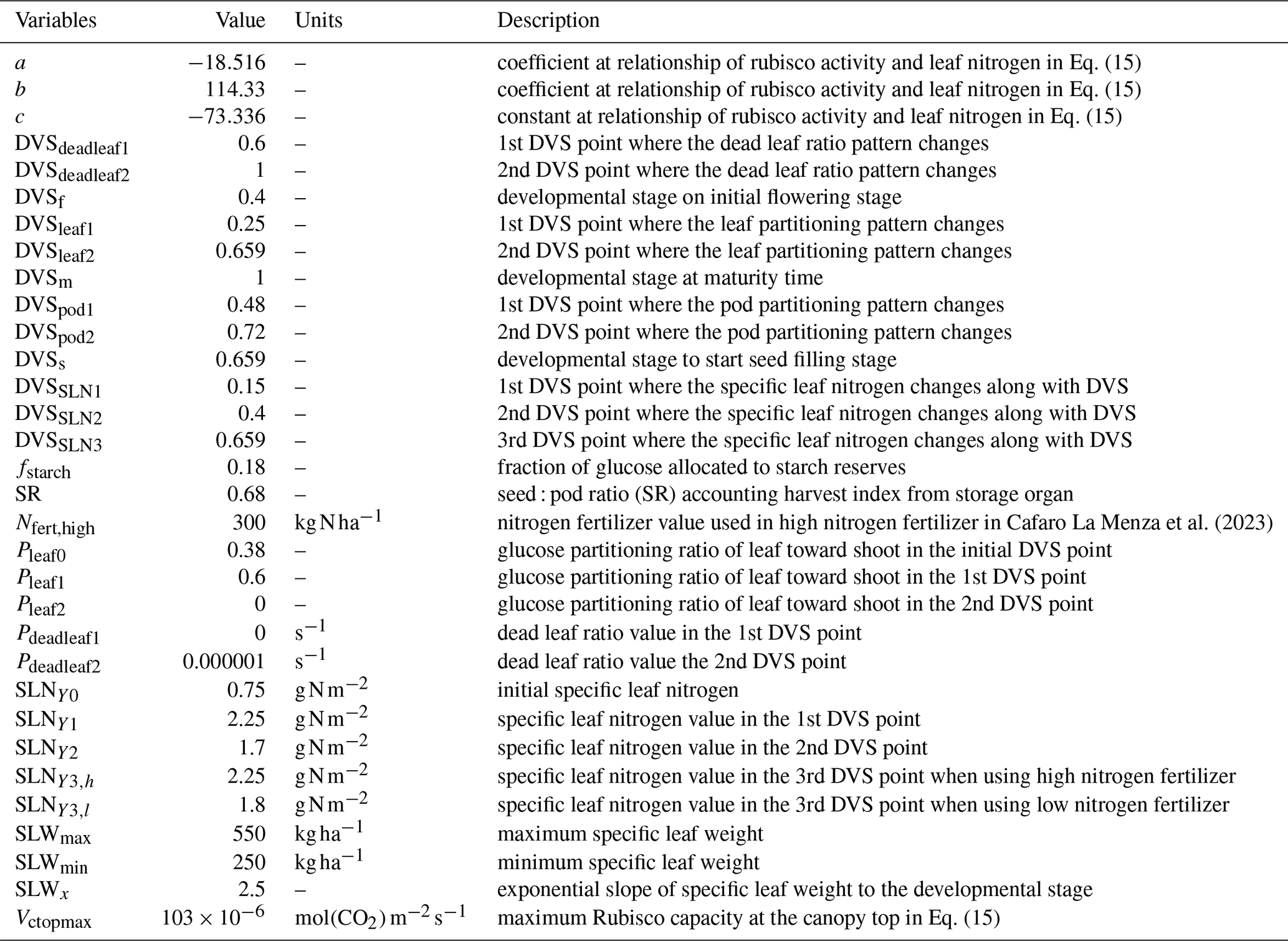
SLN values vary across different phenological stages, as the developmental stage (DVS) of soybean plants progresses from 0 (at sowing) to 1 (at harvest). DVS_f, DVS_s, DVS_m, and SLN_X1 are defined as the start of flowering, seed-filling, and maturity stages, and the point where the SLN pattern starts to change; with parameterized values of 0.4, 0.659, 1, and 0.15, respectively. SLN_Y0, SLN_Y1, SLN_Y2, SLN_Y3,l, and SLN_Y3,h represent SLN at the initial stage, early decline, pre-flowering increase, subsequent decline phases during the reproductive stage under no (l) and high (h) nitrogen inputs with values of 0.75, 2.25, 1.7, 0.75, and 1.8, respectively. N_fert,high refers to the high nitrogen fertilizer input used in the model for parameterization, as described in Table 2. Y is the observed gap in SLN between high- and low-nitrogen fertilizer treatments (g(N) m⁻²) (see Fig. S1 in the Supplement).

The growth stages were parameterized based on experimental datasets and align with those reported by Irmak et al. (2013), based on the growth stage classifications of Fehr and Caviness (1977). SLN primarily depends on nitrogen derived from biological fixation and soil nitrogen, either from natural sources or applied fertilizers. Nitrogen uptake, including biological nitrogen fixation and uptake from soil nitrogen, is implicitly captured through SLN that influences V_cmax (Eqs. 14 and 15), and SLN as affected by applied fertilizers (Eqs. 16 and 17).

2.4 Crop growth dynamics

The products of photosynthesis contribute to glucose reserves, which provide energy for growth during various developmental stages. The crop growth dynamics include a carbon biomass partitioning module to calculate the dry weight of each soybean organ (W_organ in kg ha⁻¹; see Eq. 18). This variable is the cumulative growth rate of dry weight (G_organ in $\mathrm{kg}{\mathrm{ha}}^{-\mathrm{1}}{\mathrm{s}}^{-\mathrm{1}}$) during the time from emergence to harvest. Further details on this module can be found in Masutomi et al. (2016a).

$$\begin{array}{}\text{(18)}& W_{\text{organ}}=f\left(G_{\text{organ}}\right)\end{array}$$

The W_organ is calculated separately for each soybean organ (i.e., leaf, stem, and pod including the seed, glucose reserves, and starch). The growth rate of dry weight (G_organ in $\mathrm{kg}{\mathrm{ha}}^{-\mathrm{1}}{\mathrm{s}}^{-\mathrm{1}}$) is calculated based on the parameters of conversion factor of dry weight from glucose to organ (F_glu-organ in $\mathrm{kg}{\mathrm{ha}}^{-\mathrm{1}}(\mathrm{kg}{\mathrm{ha}}^{-\mathrm{1}}{)}^{-\mathrm{1}}$) for leaf, stem, pod, root, and starch (listed in Table 1), and the ratio of glucose partitioned to organ (P_organ) for shoot, leaf, and pod (listed in Table 2). Shoot refers to aboveground biomass parts including the stem, leaf, and pod. G_organ is calculated for each organ and storage fraction (glucose, leaf, stem, pod, root, and starch) as described by:

$$\begin{array}{}\text{(19)}& {\displaystyle }& {\displaystyle }{G}_{\text{glu}}=f(W_{\text{leaf}}{A}_{\text{glu}},R_{\text{glu}})\text{(20)}& {\displaystyle }& {\displaystyle }{G}_{\text{leaf}}=G_{\text{glu}}{P}_{\text{shoot}}{P}_{\text{leaf}}{F}_{\text{glu-leaf}}\text{(21)}& {\displaystyle }& {\displaystyle }\begin{array}{rl}{\displaystyle }{G}_{\text{stem}}=& {\displaystyle }{G}_{\text{glu}}{P}_{\text{shoot}}(P_{\text{leaf}}-P_{\text{pod}})\\ {\displaystyle }& {\displaystyle }\times (\mathrm{1}-f_{\text{starch}})F_{\text{glu-stem}}\end{array}\text{(22)}& {\displaystyle }& {\displaystyle }{G}_{\text{pod}}=G_{\text{glu}}{P}_{\text{shoot}}{P}_{\text{pod}}{F}_{\text{glu-pod}}\text{(23)}& {\displaystyle }& {\displaystyle }{G}_{\text{root}}=G_{\text{glu}}(\mathrm{1}-P_{\text{shoot}})F_{\text{glu-root}}\text{(24)}& {\displaystyle }& {\displaystyle }{G}_{\text{starch}}=G_{\text{glu}}{P}_{\text{shoot}}(P_{\text{leaf}}-P_{\text{pod}})f_{\text{starch}}{F}_{\text{glu-starch}}\end{array}$$

where G_glu ($\mathrm{kg}{\mathrm{ha}}^{-\mathrm{1}}{\mathrm{s}}^{-\mathrm{1}}$) is the amount of glucose partitioned to soybean organs and reserves derived from a function of leaf dry weight (W_leaf in kg ha⁻¹), net carbon assimilation in glucose form (A_glu in $\mathrm{kg}\left(\mathrm{C}{\mathrm{H}}_{\mathrm{2}}\mathrm{O}\right){\mathrm{ha}}^{-\mathrm{1}}{\mathrm{s}}^{-\mathrm{1}}$), and glucose remobilized from starch reserves in the stem (R_glu in $\mathrm{kg}{\mathrm{ha}}^{-\mathrm{1}}{\mathrm{s}}^{-\mathrm{1}}$); A_glu is A_n that has been already converted from CO₂ to glucose using the conversion factor 1.08×10⁶ [$\mathrm{kg}{\mathrm{ha}}^{-\mathrm{1}}{\mathrm{h}}^{-\mathrm{1}}(\mathrm{mol}{\mathrm{m}}^{-\mathrm{2}}{\mathrm{s}}^{-\mathrm{1}}{)}^{-\mathrm{1}}$], which is the physical and chemical constant for the conversion; and R_glu is glucose remobilized from starch reserves in the stem, calculated using the ratio of the remobilization value. The R_glu is subtracted from the dry weight of starch reserves (W_starch). f_starch [$\mathrm{kg}{\mathrm{ha}}^{-\mathrm{1}}(\mathrm{kg}{\mathrm{ha}}^{-\mathrm{1}}{)}^{-\mathrm{1}}$] is the fraction of glucose allocated to starch reserves, calculated as stem dry weight loss.

Table 1 Crop-specific parameters used for MATCRO-Soy.

Table 2 Parameterized variables for soybean in MATCRO.

As shown in Eqs. (20)–(24), G_organ was calculated based on the conversion factor of dry weight (F_glu-organ) and ratio of glucose partitioned to that organ (P_organ). The calculations for P_organ are shown in Eqs. (25)–(27):

$$\begin{array}{}\text{(25)}& {\displaystyle }& {\displaystyle }{P}_{\text{shoot}}=\left\{\begin{array}{l}\mathrm{1}-P_{\text{root}},\text{if DVS}=\mathrm{0}\\ {\displaystyle \frac{\mathrm{1}-P_{\text{root}}({\text{DVS}}_{\mathrm{m}}-\text{DVS})}{{\text{DVS}}_{\mathrm{m}}}},\\ \text{if 0}<\text{DVS}<{\text{DVS}}_{\mathrm{m}}\\ \mathrm{1},\text{if DVS}\ge {\text{DVS}}_{\mathrm{m}}\end{array}\right.\text{(26)}& {\displaystyle }& {\displaystyle }{P}_{\text{leaf}}=\left\{\begin{array}{l}{P}_{\text{leaf0}}+{\displaystyle \frac{\text{DVS}}{{\text{DVS}}_{\text{leaf1}}}}(P_{\text{leaf1}}-P_{\text{leaf0}}),\\ \text{if DVS}<{\text{DVS}}_{\text{leaf1}}\\ P_{\text{leaf2}}-{\displaystyle \frac{(P_{\text{leaf2}}-P_{\text{leaf1}})}{{\text{DVS}}_{\text{leaf2}}-{\text{DVS}}_{\text{leaf1}}}}({\text{DVS}}_{\text{leaf2}}-\text{DVS}),\\ {\text{if DVS}}_{\text{leaf1}}\le \text{DVS}<{\text{DVS}}_{\text{leaf2}}\\ \mathrm{0},\text{if DVS}\ge {\text{DVS}}_{\text{leaf2}}\end{array}\right.\text{(27)}& {\displaystyle }& {\displaystyle }{P}_{\text{pod}}=\left\{\begin{array}{l}\mathrm{0},\text{if DVS}<{\text{DVS}}_{\text{pod1}}\\ {\displaystyle \frac{\text{DVS}-{\text{DVS}}_{\text{pod1}}}{{\text{DVS}}_{\text{pod2}}-{\text{DVS}}_{\text{pod1}}}},\\ {\text{if DVS}}_{\text{pod1}}\le \text{DVS}<{\text{DVS}}_{\text{pod2}}\\ \mathrm{1},\text{if DVS}\ge {\text{DVS}}_{\text{pod2}}\end{array}\right.\end{array}$$

P_leaf0, P_leaf1, P_leaf2 represent the leaf:shoot glucose partitioning ratio when leaf growth first starts to decline (leaf0), leaves stop growing (leaf1), and at maturity (leaf2), respectively. DVS_pod1and DVS_pod2 indicate the DVS values at which the pod:shoot glucose partitioning ratio begins to increase and eventually saturates, respectively (Fig. 2). Figure 2 in Sect. 3.2 visually represents the glucose partitioning ratio during crop growth as calibrated in this study.

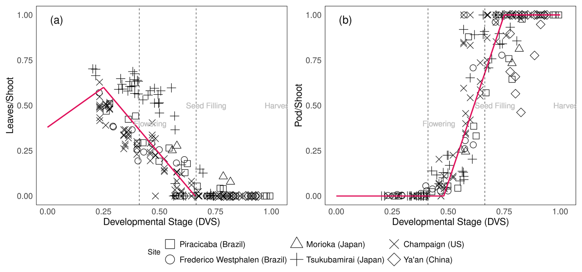
Figure 2 Glucose partitioning ratio to leaf from shoot (a) and glucose partitioning ratio to pod from shoot (b) during soybean plant development [$\text{DVS}=\mathrm{0}\left(\text{sowing}\right)-\mathrm{1}\left(\text{maturity}\right)$] at different experimental sites (square: Piracicaba, circle: Frederico Westphalen, triangle: Morioka, plus: Tsukubamirai, cross: Champaign, diamond: Ya'an. Red lines are segmented lines used for glucose partitioning in MATCRO-Soy. Dashed lines mark flowering, seed filling, and harvest times averaged across all experimental datasets.

During the calibration process, the glucose partitioned to each organ was adjusted for each developmental stage on the basis of experimental data, as further described in Sect. 3. However, in this module, the leaf dry weight decreases because of senescence. This is calculated as the loss of leaf dry weight (L_leaf in $\mathrm{kg}{\mathrm{ha}}^{-\mathrm{1}}{\mathrm{s}}^{-\mathrm{1}}$) derived from the calibration of the ratio of glucose partitioned into the dead leaf (P_dleaf in s⁻¹), as outlined in Eqs. (28) and (29).

$$\begin{array}{}\text{(28)}& {\displaystyle }& {\displaystyle }{L}_{\text{leaf}}=\left\{\begin{array}{l}\mathrm{0},\text{if DVS}<{\text{DVS}}_{\text{deadleaf1}}\\ P_{\text{dleaf}}(W_{\text{leaf}}+W_{\text{glu}}),\\ \text{if DVS}\ge {\text{DVS}}_{\text{deadleaf1}}\end{array}\right.\text{(29)}& {\displaystyle }& {\displaystyle }{P}_{\text{dleaf}}=P_{\text{deadleaf2}}{\displaystyle \frac{(\text{DVS}-{\text{DVS}}_{\text{deadleaf1}})}{(\mathrm{1}-{\text{DVS}}_{\text{deadleaf1}})}}\end{array}$$

The leaf area index (LAI) represents the leaf surface area relative to the ground area, calculated using Eq. (30). It directly influences the plant's ability to intercept solar radiation for photosynthesis.

$$\begin{array}{}\text{(30)}& \text{LAI}={\displaystyle \frac{W_{\text{leaf}}+W_{\text{glu}}}{\text{SLW}}}\end{array}$$

LAI is calculated from the estimated leaf dry weight (W_leaf, in kg ha⁻¹) and glucose reserves in leaves (W_glu, in kg ha⁻¹) divided by the specific leaf weight (SLW, in kg ha⁻¹). Glucose reserves are added to the leaf dry weight as a buffer, and affect leaf growth by storing carbohydrates that are not immediately required. SLW is the leaf dry weight per unit leaf area. The value of SLW dynamically changes during development according to the following exponential relationship:

$$\begin{array}{}\text{(31)}& \begin{array}{rl}{\displaystyle }\text{SLW}=& {\displaystyle }{\text{SLW}}_{max}+({\text{SLW}}_{\text{min}}-{\text{SLW}}_{max})\\ {\displaystyle }& {\displaystyle }\times \exp (-{\text{SLW}}_x\text{DVS})\end{array}\end{array}$$

where SLW_max, SLW_min, and SLW_x represent the maximum, minimum, and slope parameters, respectively, that define the values observed in the exponential relationship based on the experimental dataset summarized in Table 3.

2.5 Soybean yield estimation

Soybean yield is calculated from the pod dry weight at harvest (W_podharvest, in kg ha⁻¹) multiplied by the seed ratio parameter (SR), as given in Eq. (32).

$$\begin{array}{}\text{(32)}& \text{Yield}=W_{\text{podharvest}}\times \text{SR}\end{array}$$

SR was derived from experimental datasets summarized in Table 3 and represents the ratio of yield (seed, kg ha⁻¹) to W_podharvest at harvest time.

Table 3 Information about field experiments: Location, crop season, soybean variety and maturity group, water management, and nitrogen fertilizer, as well as the number of experiments for calibrating glucose partitioning ratio and evaluating soybean yield simulations.

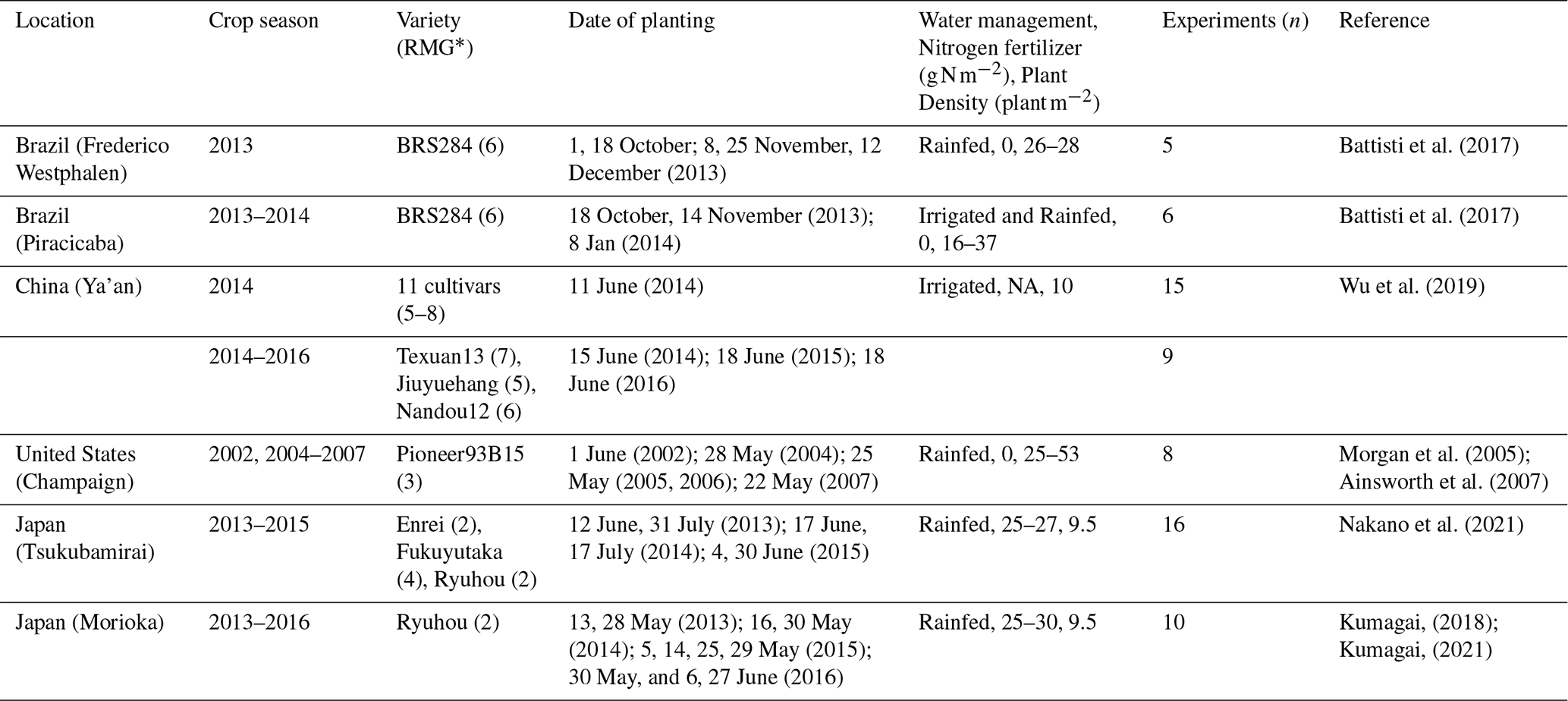
^* Relative maturity group.

2.6 Soybean-specific parameters

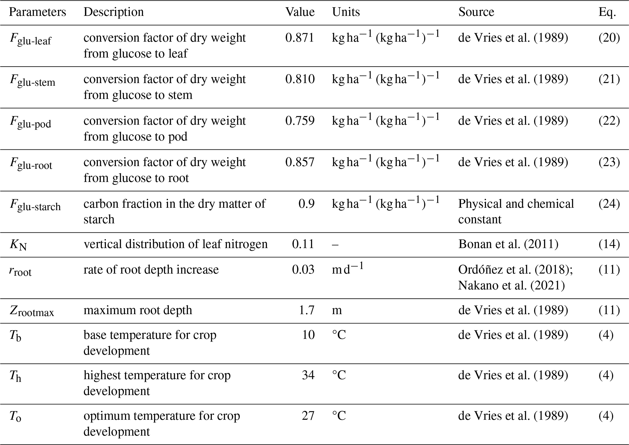
MATCRO-Soy shares several parameters with MATCRO-Rice because both plants are C₃ species. However, unlike cereal crops, soybean plants can fix nitrogen. This characteristic is represented through changes in SLN during crop growth, as described in Eqs. (16) and (17). The crop-specific parameters reflect the unique physiological and chemical processes involved in soybean growth, but still align with the general framework of MATCRO-Rice. Key parameter adjustments are outlined in Table 1, where MATCRO employs a set of specific parameters to simulate crop growth and yield. These parameters include factors related to carbon allocation, root growth characteristics, and crop development based on cardinal temperatures. By accurately representing the unique physiological and biochemical characteristics of soybean plants, these parameters improve the precision of the model in predicting soybean yield.

MATCRO-Soy is intended for use in global-scale simulations; hence, it uses a single global parameterization as a standardized set of parameters applied worldwide. It uses a unified approach for modelling crop behaviour across different regions. It is assumed that the parameter values from the different treatments and cultivars are independent. Table 2 lists variables parameterized within the model, including glucose partitioning, nitrogen, and photosynthetic capacity variables. Through the parameterization of these variables, the model can be adapted for various growing conditions and employed to assess the sensitivity of crop performance to different factors. These parameters are commonly used to evaluate the crop model's sensitivity to environmental changes and require further fine-tuning, as highlighted by simulations using other crop models (Battisti et al., 2018a).

3 Model calibration

The model's parameters were tuned using observed values for phenology and seasonality of biomass development. Once calibration was complete, the model continued to simulate crop growth, which encompasses phenological development, carbon assimilation, assimilate partitioning, and crop yield. We conducted calibrations to include various environmental conditions and soybean varieties documented in previous experimental studies as detailed in Sect. 3.1 and Table 3. The model calibration included parameterizing the dynamic biomass growth partitioning ratio for each organ (P_organ), leaf senescence, and specific leaf weight at each DVS. Other calibrations using the experimental dataset included the phenological stage, and the seed:pod ratio (SR). The crucial phenological stages (e.g., flowering and seed-filling) were calculated as the average value of the reported values in the experimental dataset. MATCRO applies this crop growth module following the method of the school of de Wit, comparing biomass growth with the observed values at various developmental stages. Shifts in partitioning and growth patterns were identified and used as reference points in the parameterization.

3.1 Description of site data used for calibration

The calibration process used experimental datasets reported in previous studies. The data were collected in field experiments across six different sites in four countries: Frederico Westphalen and Piracicaba (Brazil), Ya'an (China), Champaign (United States of America, US), Morioka and Tsukubamirai (Japan) (Table 3). The soybean cultivars grown at these experimental sites represented different maturity groups. A variety of management practices related to water management and nutrients were used in the field experiments. The farming practices differed among countries. The soybean plants were cultivated with a low planting density in China and Japan, but typically at higher planting densities in the US and Brazil. Nitrogen fertilizers were applied at most sites, but the mineral nitrogen content in soil at sites in Brazil and the US was sufficient to support crop growth. Soybean crops were planted between May and June in the US, China, and Japan, but in October or November in Brazil.

Weather data were derived from the records at the meteorological station nearest to the experimental site. The climatic conditions at the respective sites were as follows: daily mean air temperature ranges during the growing season of 18–30 °C in Frederico Westphalen (Brazil), 19–31 °C in Piracicaba (Brazil), 17–27 °C in Tsukubamirai (Japan), 14–25 °C in Morioka (Japan), 18–26 °C in Ya'an (China), and 15–28 °C in Champaign (US). The seasonal precipitation (mm) was 1669 mm in Frederico Westphalen (Brazil), 679 mm in Piracicaba (Brazil), 453 mm in Morioka (Japan), 865 mm in Tsukubamirai (Japan), 1012 mm in Ya'an (China), and 787 mm in Champaign (US). The amount of solar radiation also differed among the experimental sites; China received the least solar radiation and Brazil received the most during the experimental period (Fig. S2 in the Supplement). These data represent the diverse climatic conditions in soybean-producing countries. The field data used for calibration were collected across multiple crop seasons, specifically from 2002, 2003–2007 and from 2013–2016. These time periods were expected to capture the current climatic and environmental variability.

3.2 Biomass partitioning and specific leaf weight

The MATCRO-Soy model represents carbon assimilation by incorporating the carbon fraction in dry matter and that in glucose allocated to various plant organs. The glucose ratio for each organ was parameterized based on measurements of leaf weight, leaf senescence, stem weight, pod weight, and specific leaf weight across different developmental stages. To simulate glucose partitioning, we used Eqs. (25)–(29) to fit the segmented linear functions to the experimental dataset (Figs. 2 and 4) and the parameter values as shown in Table 2, as this value is used to obtain the average value of soybean partitioning behaviour. The segmented linear functions for glucose partitioning were manually determined by visual inspections of the plot. This approach was chosen because of the challenges in applying nonlinear optimization. Breakpoints in the developmental stage were determined based on assumed growth characteristics, such as the decrease in leaf development after the seed-filling stage and the start of pod formation after flowering. We assumed an increasing trend of glucose allocation to leaf and shoot development during the early stage when data were unavailable, with subsequent segments aligned with observed data trends. The calibrated glucose partitioning ratio varied across the varieties and environmental conditions and was derived by converting biomass growth into glucose allocation as outlined in Eqs. (19)–(24).

The parameterization reflected the observed data, as well as the linear growth of leaves and pods during the developmental stages. It was used for seed : pod ratio and phenology parameterization. The dashed lines in Figs. 2 and 3 indicate the estimated flowering and seed-filling stages, as determined by calculating the average time of phenological stages across all the experimental datasets. The independent dataset was used for evaluating the calibrated model at the point-scale level. After removing the calibration data, the simulated yield at the site scale showed a correlation coefficient of 0.68 and significant consistency (p-value<0.001) with observed data (Fig. S3 in the Supplement). The simulated data were also consistent with observed data for aboveground biomass weight, pod weight, and leaf area index, with correlation coefficients of 0.60–0.90.

Assimilated carbon is subsequently allocated to other parts of the plant. Compared with varieties grown at other sites, the soybean varieties grown in Tsukubamirai (Japan) tended to have lower partitioning to the stem during the vegetative stage. The ratio of glucose to leaves in Sichuan (China) was unexpectedly high near maturity in 2016, resulting in a low level of partitioning to pods because of low temperature and drought conditions. The storage organ biomass increases during the reproductive stage to produce pods and seeds, whereas the shoot senesces at the end of the maturity period. Hence, yield is estimated using seed weight (as determined by storage organ weight) and the parameterized seed:pod ratio. In Champaign (US), pod partitioning tended to occur early during pod initiation in early maturing varieties. It is also observed in another study as the dry weight of pods before the seed filling stage was relatively high in early maturing varieties (Kawasaki et al., 2018). Early pod initiation occurred in the soybean variety “Ryuhou” in Tsukubamirai in 2013 (Nakano et al., 2021). The dead leaf ratio parameter indicates the degree of leaf senescence after the seed-filling stage (Fig. 3), as calculated from the amount of leaf loss observed during the growing season.

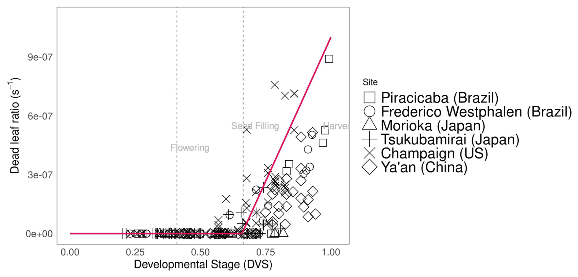
Figure 3 Dead leaf ratio (s⁻¹) during soybean plant development ($\text{DVS}=\mathrm{0}-\mathrm{1}$). Abbreviations and symbols are the same as in Fig. 2.

Specific leaf weight (SLW) is a significant parameter in crop growth parameterization and was calibrated to follow the measured data shown in Fig. 4. We used the measured leaf weight and leaf area index data from the experimental datasets described in 2.4 and Eq. (30) to calculate the ratio of leaf weight to leaf area (SLW) during different phenological stages. These ratios change over time, and vary among growing seasons and cultivars (Thompson et al., 1996; Slattery et al., 2017). In the figure, SLW from Champaign (US) was excluded because of discrepancies in the timing of leaf area and leaf weight biomass measurements. While the SLW varied among the sites, we fitted the model of SLW assuming a saturating exponential function of developmental stage (red line in Fig. 4). This pattern aligned well with the biological process, i.e., the SLW initially increases because of rapid biomass accumulation but saturates as the leaves mature.

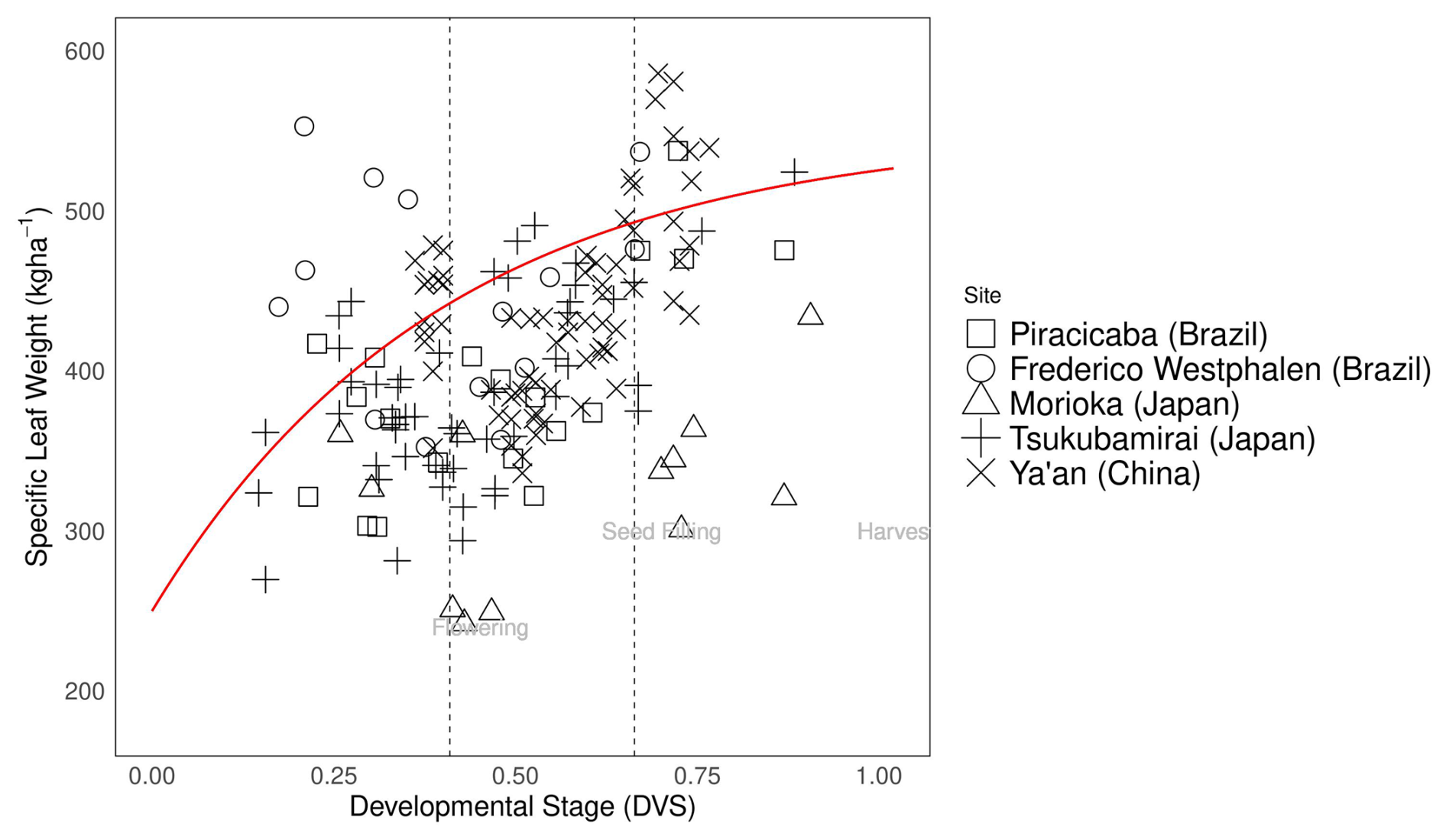
Figure 4 Specific leaf weight (kg ha⁻¹) during soybean plant development ($\text{DVS}=\mathrm{0}-\mathrm{1}$). Abbreviations and symbols are the same as in Fig. 2.

4 Model evaluation setup

MATCRO was developed in FORTRAN and coupled with the global climate model's output, simulated at a spatial resolution of 0.5°×0.5° and hourly–daily temporal resolution. The output of the model is gridded crop yield (kg ha⁻¹) as stored in netCDF file format in a global map with one harvest simulated per year. We evaluated the model's performance at global, country, and grid-cell levels for 34 years (1981–2014) at 0.5° spatial resolution with yearly harvested yield output. The accuracy of the simulated yield was assessed by comparison with reference global and country-level data from the Food and Agriculture Organization (FAOSTAT, 2024). The simulated grid-cell level yield was compared with Global Dataset of Historical Yield (GDHY) data, which are derived from statistical records, FAO data, and remote sensing data (Iizumi, 2019).

4.1 Simulation settings and data inputs

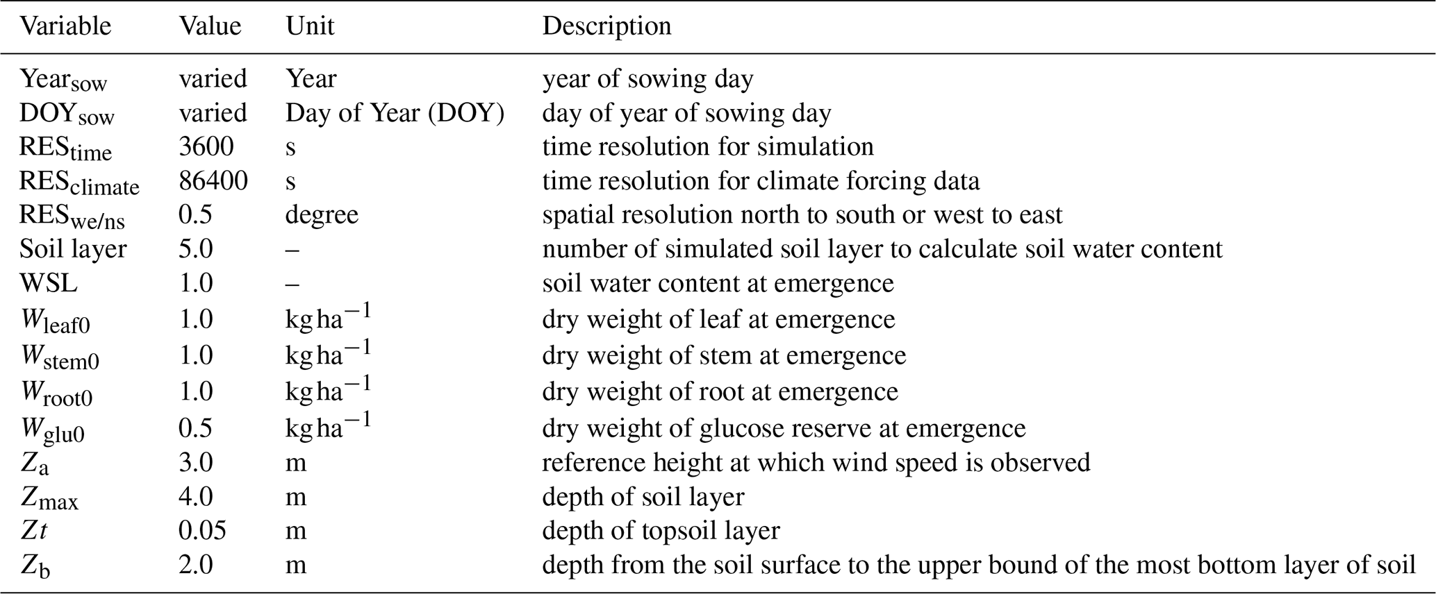
The parameters were set as shown in Table 4, covering the period of sowing years from 1980–2014, with various planting times across different regions. The model incorporated global daily climate data (86 400 s) as input data. Although the simulation framework was that of the established MATCRO-Rice v.1 (Masutomi et al., 2016b), several modifications were made to enhance its applicability at a global scale. Notably, the temporal resolution was adjusted from half-hourly (1800 s) to hourly (3600 s), allowing the model to maintain consistency in capturing critical processes such as diurnal variations in photosynthesis and transpiration, while optimizing computational efficiency. These adjustments ensured that the model was suitable for large-scale simulations while preserving essential physiological processes.

Table 4 Parameter settings for simulation.

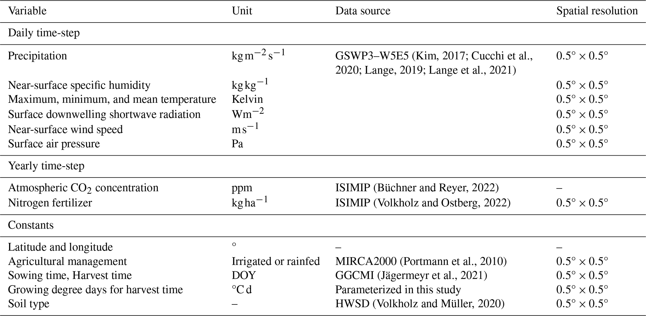
The model simulates soybean yield using input data as described in Table 5. It uses the following global input data: crop calendar from the Global Gridded Crop Model Intercomparison (GGCMI), which separates rainfed and irrigated systems; atmospheric CO₂ and climate data from the Inter-Sectoral Impact Model Intercomparison Project (ISIMIP), which provides bias-adjusted climate input data for historical data (GSWP3-W5E5 v2.0); soil classifications from the Harmonized World Soil Database (HWSD v1.2); and nitrogen fertilization for C₃ fixing crops of the ISIMIP, which is derived from the land use dataset (Hurtt et al., 2020). ISIMIP bias-adjusted data are used to maintain uniformity in the climate impact data across sectors and scales in the framework. This dataset, which is provided by ISIMIP, has a spatial resolution of 0.5° . To determine the growing degree days for maturity, we considered the phenological maturity time from the GGCMI crop calendar for harvest time and global ISIMIP climate data over 10 years (2000–2010) to capture the shifts in variability across the current evaluation years.

Table 5 Data input for MATCRO simulation.

4.2 Global yield evaluation methods

In this study, we assessed the statistical relationship between simulated yields and observed or reference data using the common metrics of Pearson's correlation coefficient (corr) as calculated using Eq. (33) with significance level (p-value), agreement between the simulated and observed results using root mean square error (RMSE) as calculated using Eq. (34), and relative bias, as calculated using Eq. (35), for time-series yield data as follows:

$$\begin{array}{}\text{(33)}& {\displaystyle }& {\displaystyle }\text{corr}={\displaystyle \frac{{\sum }_{i=\mathrm{1}}^n(X_i-\stackrel{\mathrm{‾}}{X})(Y_i-\stackrel{\mathrm{‾}}{Y})}{\sqrt{{\sum }_{i=\mathrm{1}}^n(X_i-\stackrel{\mathrm{‾}}{X}{)}^{\mathrm{2}}(Y_i-\stackrel{\mathrm{‾}}{Y}{)}^{\mathrm{2}}}}}\text{(34)}& {\displaystyle }& {\displaystyle }\text{RMSE}=\sqrt{{\displaystyle \frac{\mathrm{1}}{n}}\sum _{i=\mathrm{1}}^n(X_i-Y_i{)}^{\mathrm{2}}}\text{(35)}& {\displaystyle }& {\displaystyle }\text{relative bias}={\displaystyle \frac{\mathrm{1}}{n}}\sum _{i=\mathrm{1}}^n|X_i-Y_i|\times {\displaystyle \frac{\mathrm{1}}{\stackrel{\mathrm{‾}}{Y}}}\end{array}$$

where X_i and Y_i indicated simulated and observed values for each measurement; $\stackrel{\mathrm{‾}}{X}$ and $\stackrel{\mathrm{‾}}{Y}$ denote the mean of simulated and observed values for the harvested year annually; and i and n are the ith data point and total number of data, respectively. We used n=34 year for global-scale data, while the output after calibration was evaluated at the point-scale using $n=\mathrm{14}-\mathrm{122}$ of the available experimental datasets.

Detrended yield represents the time-series yield data for both simulated and observed values after removing the linear trend by subtracting the slope and intercept of the fitted linear regression (long-term yield trend). This approach enables the separation of short-term yield fluctuations from systemic long-term shifts. To provide a clear interpretation of the model's evaluation errors, yield fluctuations were evaluated separately for the long-term and detrended data using mean squared deviation (MSD) and its components (Gauch et al., 2003; Kobayashi and Salam, 2000), as outlined in Eq. (36):

$$\begin{array}{}\text{(36)}& {\text{MSD}}_{\mathrm{y}}={\text{SB}}_{\mathrm{y}}+{\text{SDSD}}_{\mathrm{y}}+{\text{LCS}}_{\mathrm{y}}\end{array}$$

where MSD_y is the square of RMSE for each long-term yield trend or detrended yield. Its components include mean squared bias (SB_y), difference in the magnitude of fluctuation, namely the squared difference between standard deviations (SDSD_y), and the lack of positive correlation weighted by the standard deviations (LCS_y) as proposed by Kobayashi and Salam (2000). These terms were calculated using Eqs. (37)–(41), as follows:

$$\begin{array}{}\text{(37)}& {\displaystyle }& {\displaystyle }{\text{SB}}_{\mathrm{y}}={\left(\stackrel{\mathrm{‾}}{X}-\stackrel{\mathrm{‾}}{Y}\right)}^{\mathrm{2}}\text{(38)}& {\displaystyle }& {\displaystyle }{\text{SDSD}}_{\mathrm{y}}={\left({\text{SD}}_X-{\text{SD}}_Y\right)}^{\mathrm{2}}\text{(39)}& {\displaystyle }& {\displaystyle }{\text{SD}}_X=\sqrt{{\displaystyle \frac{\mathrm{1}}{n}}\sum _{i=\mathrm{1}}^n{\left(X_i-\stackrel{\mathrm{‾}}{X}\right)}^{\mathrm{2}}}\text{(40)}& {\displaystyle }& {\displaystyle }{\text{SD}}_Y=\sqrt{{\displaystyle \frac{\mathrm{1}}{n}}\sum _{i=\mathrm{1}}^n{\left(Y_i-\stackrel{\mathrm{‾}}{Y}\right)}^{\mathrm{2}}}\text{(41)}& {\displaystyle }& {\displaystyle }{\text{LCS}}_{\mathrm{y}}={\text{SD}}_X{\text{SD}}_Y(\mathrm{1}-\text{corr})\end{array}$$

Higher SB_y, SDSD_y, and LCS_y indicate that model failed to simulate the mean of the measured yield, magnitude of fluctuation around the mean yield, and pattern of fluctuation in yield across n measurements, respectively. SD_X and SD_Y denote the standard deviation of simulated (X) and observed values (Y), respectively, and LCS_y depends on the correlation coefficient (corr).

5 Evaluation of model performance

We calculated soybean yield with a global-scale map based on the gridded data of irrigated and rainfed area from the MIRCA2000 dataset, which represents global agricultural land use around the year 2000 (Portmann et al., 2010), to get the actual yield value. We evaluated yield during the period of 1981–2014 because the MIRCA dataset was available within that period. The simulated yield at the global scale, and at the country scale for regional comparison, was determined by aggregating grid cell data to compute the mean soybean harvested area within each country grid as described below in Eq. (42):

$$\begin{array}{}\text{(42)}& \begin{array}{rl}{\displaystyle }& {\displaystyle }{\text{Yield}}_{\text{region}}=\\ {\displaystyle }& {\displaystyle \frac{{\sum }_{i=\mathrm{1}}^n\left[\right({\text{Yield}}_{\text{rf}}{)}_i({\text{Area}}_{\text{rf}}{)}_i+({\text{Yield}}_{\text{ir}}{)}_i\left({\text{Area}}_{\text{ir}}{)}_i\right]}{{\sum }_{i=\mathrm{1}}^n\left[\right({\text{Area}}_{\text{rf}}{)}_i+\left({\text{Area}}_{\text{ir}}{)}_i\right]}}\end{array}\end{array}$$

where Yield_region is the aggregated yield in a given region (country or global-scale) in kg ha⁻¹ from the grid cell number (i) ranging from 1 to n (total number of grid cells in the region); Yield_rf and Yield_ir are estimated yield under rainfed and irrigated conditions,and Yield_ir respectively; and Area_rf and Area_ir are the soybean rainfed and irrigated area (ha), and Area_ir respectively.

5.1 Model output yield as evaluated at the global and national scales

Figure 5a shows a time-series comparison from 1981–2014 between the global mean yields reported by FAOSTAT and those simulated by MATCRO-Soy. The results show that the model captured the upwards trend in yields over the period with a shallower slope compared with that of the reported yield data. The correlation coefficient was 0.81, and was significant (p<0.01); and the errors were RMSE of 298 kg ha⁻¹ and relative bias of 0.12. Notably, the simulated linear increase contributed to the higher correlation coefficient for the yield trends.

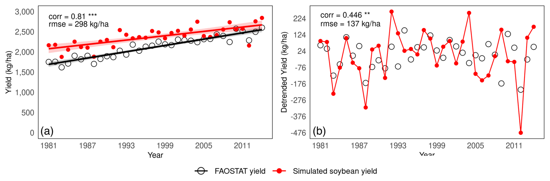
Figure 5 Time-series comparison between simulated yields by MATCRO-Soy and FAOSTAT reported yield data: (a) Global yield and long-term trend during 1981–2014, and (b) Detrended yield during 1981–2014. Correlation for detrended yield was calculated by subtracting linear trend. Symbols ***, **, and * denote p<0.001, 0.01, and 0.05, respectively.

Figure 5b compares the detrended global mean yield observed by FAOSTAT and the simulated value by MATCRO-Soy after removing the long-term linear trend across the study period. The detrended yield is the value after the long-term trend is subtracted from the original yield data. It isolates the variability primarily driven by climate fluctuations to evaluate interannual variability independent of long-term trends. However, it also removes longer-term signals (e.g., effects of technological improvements or increasing CO₂ concentrations). The correlation coefficient for the detrended yield data decreased to 0.446 (p<0.01). The model reproduced the interannual variations well with an RMSE of 137 kg ha⁻¹. Specifically, according to observed data, there were significant yield reductions in the years 1983, 1988, 2009, and 2012. Among these, the model successfully reproduced the yield reductions in three years (1983, 1988, and 2012), excluding 2009. Severe droughts occurred in those years, and the model's ability to capture these events is noteworthy.

We evaluated the model's performance for 10 major soybean-producing countries; Argentina, Brazil, China, India, Paraguay, the US, Italy, Russia, Bolivia, and Canada, which together account for 96 % of global soybean production (based on total average production from 2012–2021 reported in FAOSTAT). Figure 6 compares the simulated average yields per country and the reported average yields per country as reported in FAOSTAT for 1981–2014 with the ellipsoids indicating the distribution of the simulated yield values within the 90 % confidence range. The model reproduced the national average yield levels well for the top 10 producing countries, as indicated by a correlation coefficient of 0.519 (p<0.001) and an RMSE of 1085 kg ha⁻¹. The correlation coefficients were significant for six countries; Argentina, Brazil, India, Italy, Paraguay, and the US (see Fig. S4 in the Supplement for further evaluation of these six countries). Focusing on the US, Brazil, and Argentina, which together account for 69 % of global soybean production, the model's accuracy showed a correlation coefficient of 0.645 (p<0.001) and an RMSE of 916 kg ha⁻¹, although soybean production in Brazil was underestimated. When all 10 countries were considered, the correlation coefficient decreased to 0.291, although it remained statistically significant. These results demonstrate that the model performs reasonably well in capturing yield variations in major producing countries and achieves particularly lower bias in some countries (e.g., the US, Italy, and Canada).

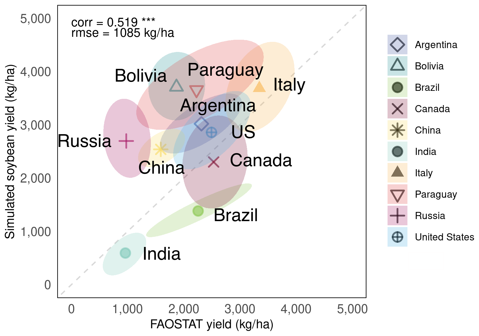
Figure 6 Comparison between average yields simulated by MATCRO-Soy and average yields reported by FAOSTAT for the 10 major soybean-producing countries during 1981–2014. Ellipsoid shows 90 % confidence range of annual yield.

A time series comparison of average yields for each of the 10 major soybean-producing countries is shown in Fig. 7. An evaluation of the long-term trends (Fig. 7a) revealed that MATCRO-Soy effectively captured the trends of increasing soybean production. The modelled and observed trends showed the strongest agreement in Brazil (0.91), followed by Argentina (0.62) and the US (0.64). The detrended yields revealed interannual variability (Fig. 7b). For these data, the modelled and observed data had the highest correlation coefficient in Paraguay (0.61), followed by the US (0.57) and Brazil (0.49), and the lowest correlation coefficients in China (0.18) and Bolivia (−0.32). These findings suggest that the model tends to perform with greater accuracy for countries with higher production levels, even in time series comparisons at the national level.

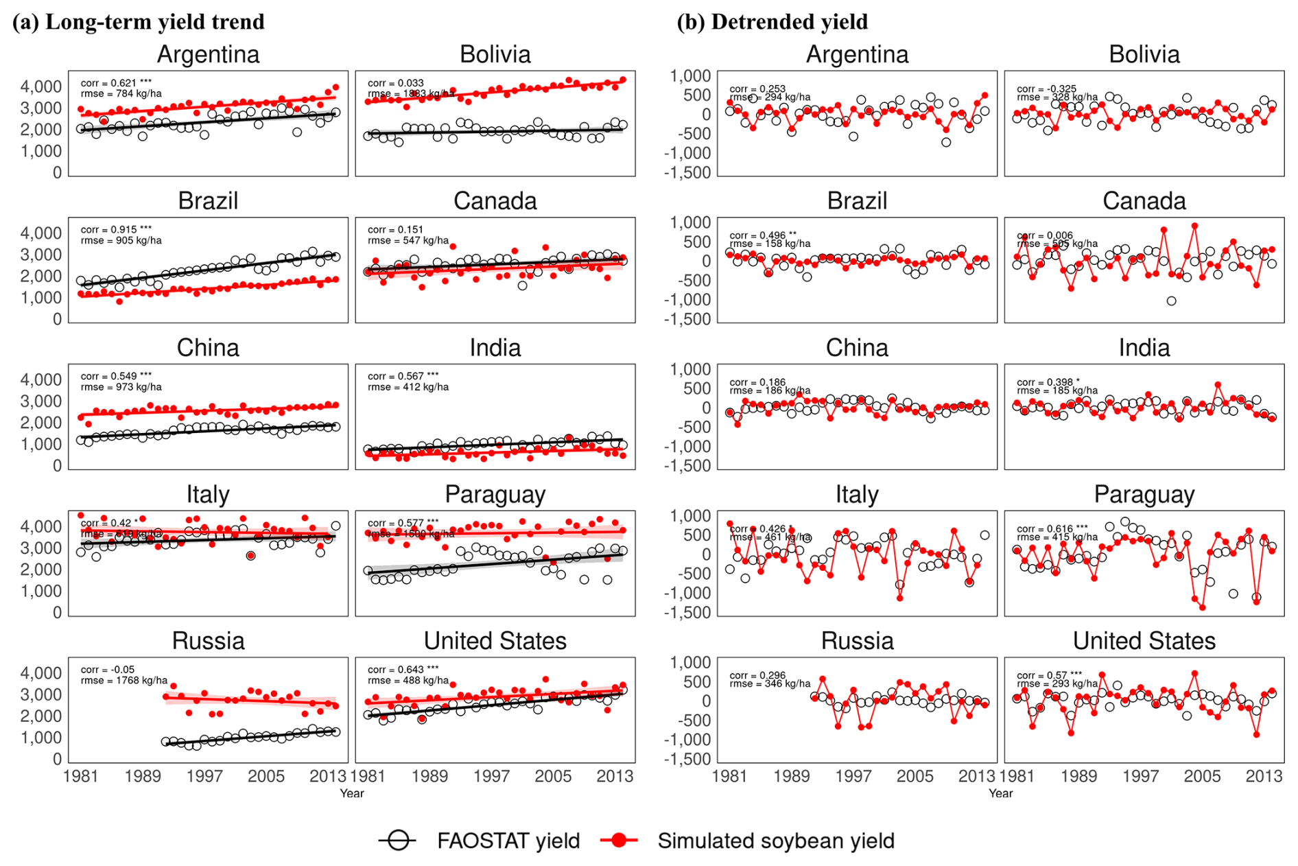
Figure 7 Time-series comparison between yields simulated by MATCRO-Soy (red circle) and yields reported by FAOSTAT (open circle) in 10 top soybean-producing countries during 1981–2014: (a) Long term yield trend in kg ha⁻¹ (solid line), (b) Detrended yield in kg ha⁻¹ after subtracting linear trend. Correlation coefficient and RMSE are shown in each panel. Symbols ***, **, and * denote p<0.001, 0.01, and 0.05, respectively. Shading near solid line is standard error with confidence interval of 95 %.

5.2 Temporal trends and variability

The model's performance was further assessed with the MSD components for yield, separated into yield, long-term yield trend, and detrended yield for both the global (Table S1 in the Supplement) and country scales (Tables S2–S4 in the Supplement). We separated the MSD into SB, SDSD, and LCS, which reflect errors in mean yield, magnitude of yield variability, and the pattern of year-to-year fluctuations, respectively. The greatest contributor to error at the global scale was SB, contributing approximately 71 % and 77 % of total MSD for yield and detrended yield, respectively (Table S1).

Figure 8 shows MSD components in the top six soybean-producing countries. In most countries, SB was the primary source of error. The highest MSD was in Paraguay, and was largely driven by SB, with a notable contribution from LCS. This indicates that the model simulated variability well but poorly captured the mean yield. The low MSD in the US was also driven by SB, but LCS also contributed to year-to-year variability. Meanwhile, LCS was the greatest contributor to yield error in Canada and Italy (Table S2) because of pronounced discrepancies in the simulated interannual variability. SDSD contributed to error only in Brazil, where the model underestimated the mean yield and the deviation. These results highlight that the mean yield bias is main source of error at the global and country scales, while LCS and SDSD contribute notably in specific regions where the model fails to capture the variability or the temporal pattern.

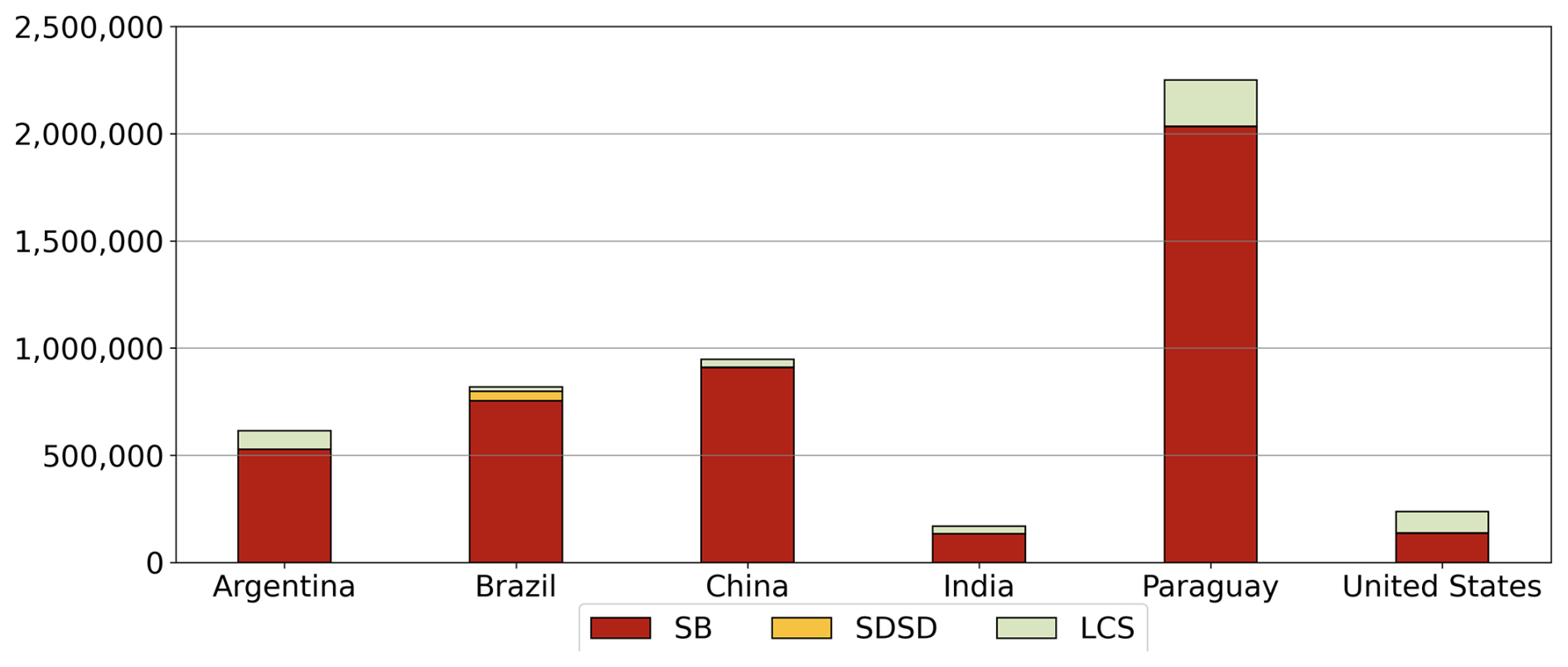
Figure 8 Mean squared deviation (MSD) components of squared bias (SB), sum of difference in standard deviation (SDSD), and lack of positive correlation (LCS) for yield error in top six soybean-producing countries.

5.3 Model performance at the grid-cell level

We evaluated MATCRO-Soy at the grid-cell level by comparing simulated yields with observed ones from the GDHY dataset reported by Iizumi (2019). Figure 9a and b show the simulated and observed yields averaged over 34 years, and Fig. 9c shows relative bias between them. Figure 10 shows the interannual correlation between simulated and observed yields for 34 years. The simulated yield was calculated for soybean-growing areas from the MIRCA2000 dataset, which offers broad spatial coverage where yield data for certain regions, including Canada, Russia, Australia, and many European and Asian countries, are missing in the GDHY dataset (Iizumi and Sakai, 2020). The density plot of the simulated yield showed more variability than did the GDHY data in Fig. 9. However, both datasets exhibited a density peak of approximately 2000–3000 kg ha⁻¹ and the simulated yield mostly overestimated the higher yield value. Figure 9a–c also show the distribution of simulated and observed yields.

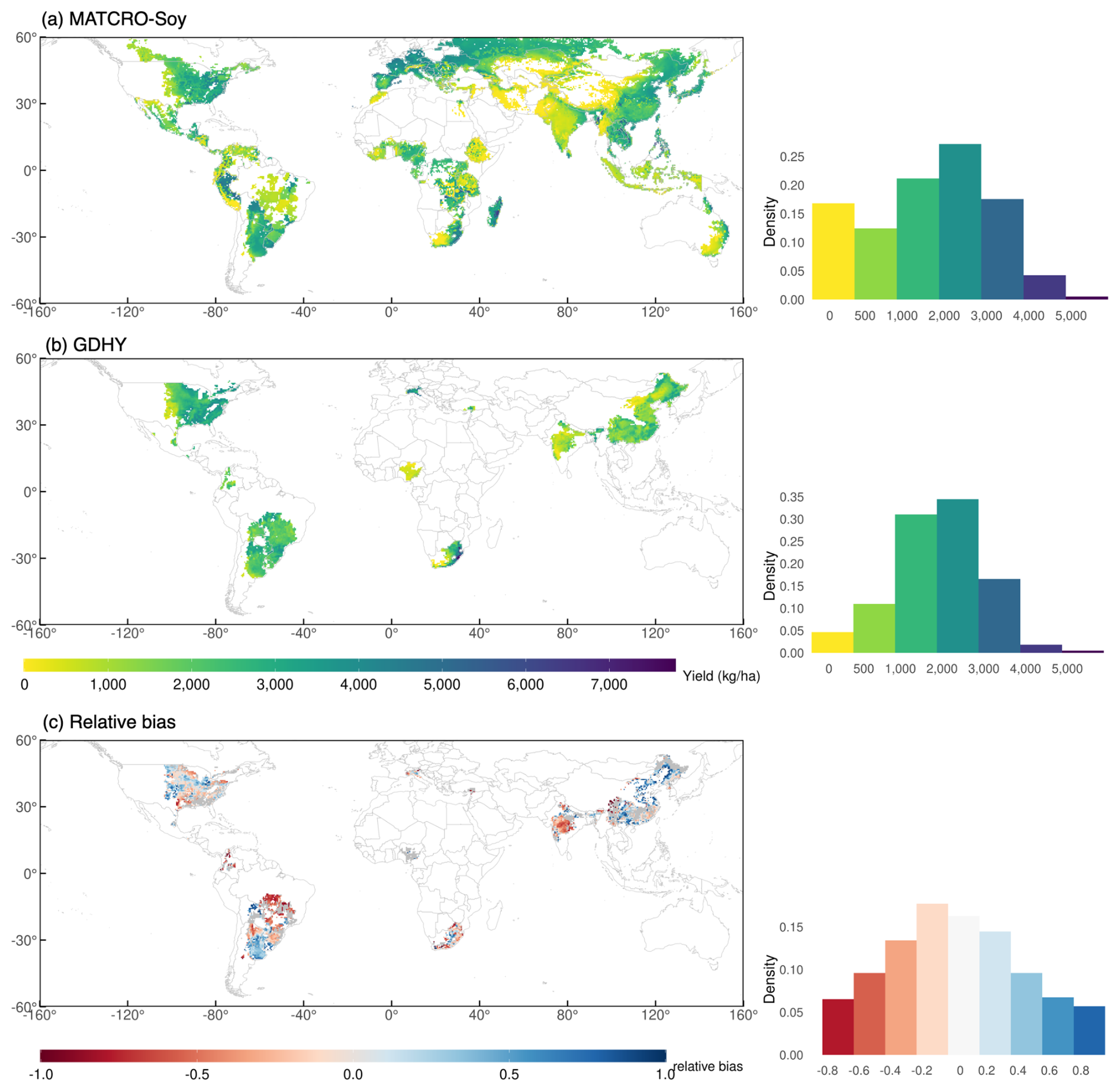
Figure 9 Global map of 34 year averaged (1981–2014) yield of GDHY dataset (a), simulated by MATCRO-Soy (b), and relative bias (c) with each density plot distribution. In (c), areas in grey are those where the correlation between simulated and observed yields was non-significant (p>0.05).

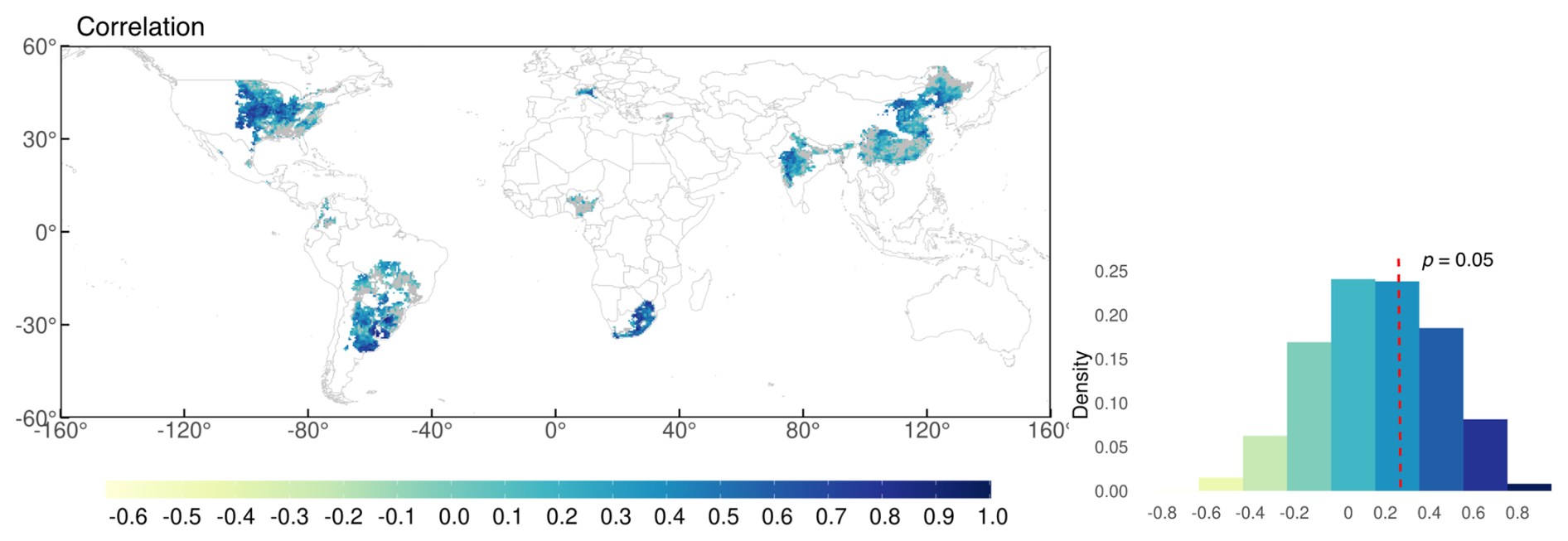
Figure 10 Time-series correlation between simulated and observed yield in 1981–2014 after removing trends from 5 year moving average (c). Grey colour depicts regions with non-significant correlations (p>0.05) in the map. Red dashed line shows the border of p=0.05 for the number of years (n=34) in the density distribution plot.

The relative bias map (Fig. 9c) highlights that overestimation was prominent in parts of South America (particularly Argentina), Russia, and China. In contrast, the model tended to underestimate yields in South Africa, India, and Brazil. Most of the grid cells in Brazil showed low yields, likely due to shorter growing periods in the input data compared with those in the field experimental data. These results aligned with the trends observed at the national scale, which were influenced by the aggregation process. During aggregation, the national-scale results represent the average performance across all grid cells, weighted by the number of grids within each region. Most grids had a relative bias of −0.2 to 0.2, accounting for 37 % of the total grid area. For areas shown in grey, the correlation was statistically insignificant. The density plot of simulated yield showed more variability compared with the GDHY data. However, both datasets exhibited a density peak at approximately 3000 kg ha⁻¹, and the simulated yield mostly overestimated the observed yield. Correlation coefficients were calculated for each grid cell between the simulated yield and the GDHY dataset after removing the moving-average to reveal interannual variation (Fig. 10). The correlation was significant in 66 % of the grid cells (p<0.05).

Figure 11 presents the relative RMSE (RMSE value compared with the observation value) between the simulated yields and GDHY datasets for detrended yield at the grid-scale. The RMSE values were relatively higher in some parts of Africa (particularly in Nigeria), the US, India, and China, and relatively lower in Brazil and Argentina. India and the US showed low RMSEs at the national-level, but some grid cells within both countries had higher relative RMSEs at the grid-cell level. Detailed information on the spatial variation in error and its components is provided in Fig. S6 in the Supplement for the long-term yield trend and Fig. S7 in the Supplement for the detrended yield.

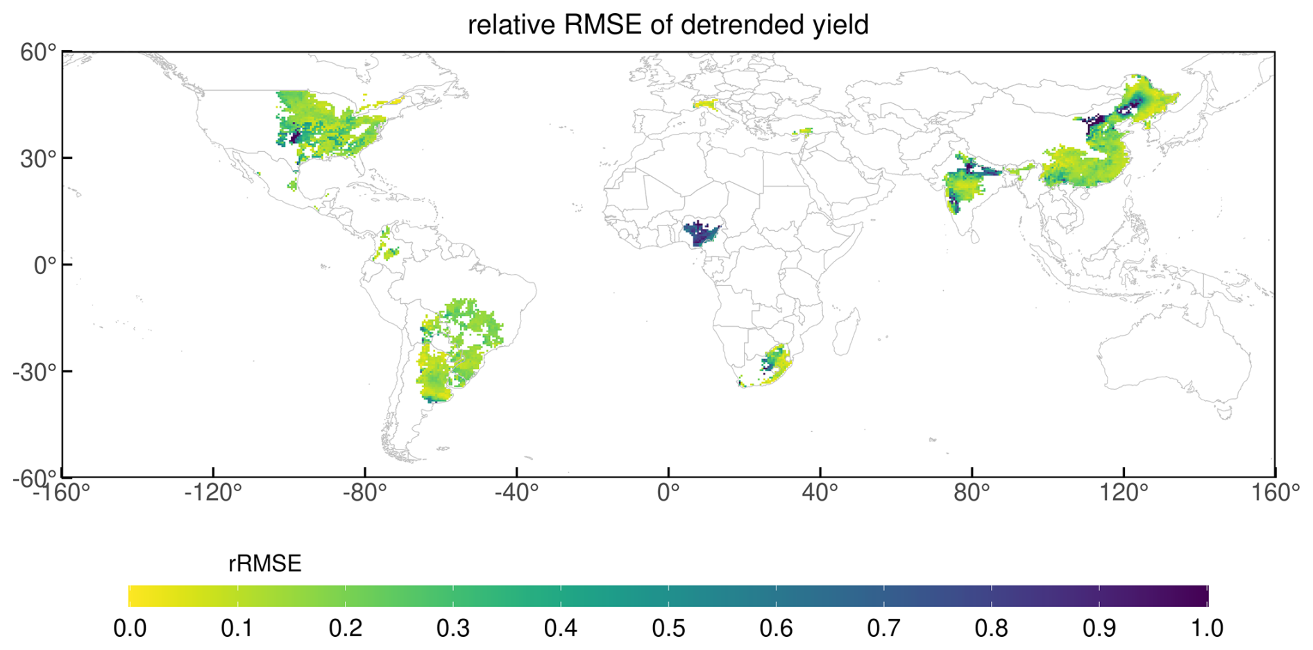
Figure 11 Relative RMSE calculation between simulated and observed yield for detrended yield at the grid-cell level.

5.4 Model performance at the leaf-level

We simulated the leaf-level variation in V_cmax at the site-scale for Champaign, US (the country with the highest soybean production), for the 2002 growing season. The global parameterization of MATCRO-Soy was used for this simulation (Fig. 12). The leaf-level simulated V_cmax values aligned closely with the measured data reported by Bernacchi et al. (2005) during the vegetative stage, but showed some deviations during the flowering to seed-filling stages (dotted line in Fig. 12). This alignment highlighted the ability of the model to represent essential photosynthetic processes influenced by leaf nitrogen content.

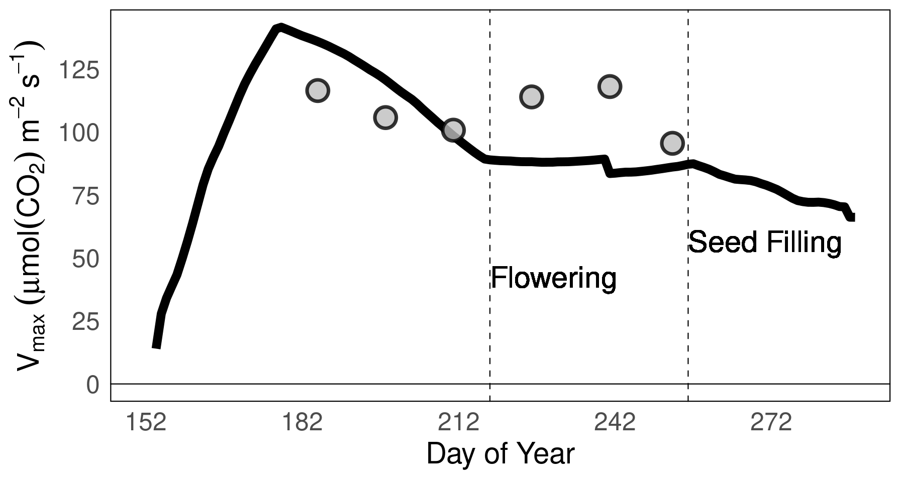
Figure 12 Maximum carboxylation capacity of Rubisco ($\mathrm{\mu }\mathrm{mol}\left({\mathrm{CO}}_{\mathrm{2}}\right){\mathrm{m}}^{-\mathrm{2}}{\mathrm{s}}^{-\mathrm{1}}$) during the growing period in Champaign (US) in 2002 as simulated using MATCRO-Soy (black line) and as measured (grey dots) by Bernacchi et al. (2005).

6 Discussion

6.1 Validation of MATCRO-Soy

In prior studies, soybean yield predictions often faced challenges in capturing crop responses to climatic variables. Our results show that the MATCRO-Soy model effectively captures the linear trend in soybean yields, with higher accuracy for long-term trends (corr=0.812) than for detrended yields (corr=0.446) (Fig. 5). This result for the global detrended yield improves upon that of the benchmark study of Müller et al. (2017), indicating that there is less variation in process-based models based on their statistical correlations. Another crop model, PRYSBI2, reached a significant correlation of 0.57 (p<0.050) based on long-term trends. However, model accuracy is enhanced when site-specific parameters are used. This has been demonstrated in regional-scale evaluations in previous studies, which were used for parameterization in this global simulation (Battisti et al., 2017; Kumagai, 2018, 2021; Morgan et al., 2005; Nakano et al., 2021; Wu et al., 2019). Those studies showed that integrating factors such as cultivar differences, ensembles of multiple crop models, nitrogen content, and more accurate measurement methods allow for a more reliable representation of local growing conditions and climate variability.

We examined the model's performance in predicting soybean yields for the 10 largest soybean-producing countries. As shown in Fig. 6, the RMSE was 1085 kg ha⁻¹ (average yield over 34 years). This value is similar to that reported in another study using the LPJ-GUESS model incorporating a biological nitrogen fixation module (Ma et al., 2022), where the RMSE was approximately 800 kg ha⁻¹ (average yield over 10 years). Evaluation of MATCRO-Soy's performance at the grid-cell level, as shown in Fig. 9, revealed that the correlation between simulated and observed yields was significant (p<0.05) in 66 % of the grid cells, with the value in most grid cells within the range of 0.2–0.6. These findings align with those of the benchmark study of Müller et al. (2017), who found that time-series correlations in GGCM-simulated soybean yields ranged from 0.25–0.65 because of various discrepancies in the data. These correlations were calculated using detrended values, which is a useful strategy for evaluating interannual variability and the model's sensitivity to climate fluctuations. However, detrending removes important long-term signals related to genetic improvements, cultivar and management changes, and/or increased CO₂ levels.

Analyses of the correlations between yield and detrended yield (Figs. 5 and 6) indicate that the model performed better (i.e., a higher correlation coefficient) when predicting long-term yield trends. MATCRO-Soy was able to capture the trend of increased atmospheric CO₂ and nitrogen fertilizer inputs, despite the interannual variability in climate conditions. Analyses of MSD and its components revealed that the lack of positive correlation was the major contributor to error in Canada and Italy among the 10 top soybean-producing countries (Table S2). The SB values were small for both Canada and Italy, suggesting that MATCRO-Soy accurately represents the average productivity despite its inability to capture the variability or amplitude of the yield trend over time within those regions. Factors such as changes in sowing date, land use, pest management, cultivar maturity group, and planting density may contribute to discrepancies in soybean yield under climate change (Battisti et al., 2018a; Marin et al., 2022). Hence, there is a need for improved parameterization to better represent the dynamics of yield variability in countries such as Canada and Italy.

The high yields in Argentina and Paraguay reflect the consistency of favourable growing conditions in those countries (Fig. 7a), particularly the alignment of daily temperatures and seasonal precipitation with critical growth stages. This result suggests that these regions are less susceptible to interannual variability, as well as being located in areas that receive more radiation for photosynthesis. The comparison of simulated and observed yields at the grid-cell level (Fig. 10) revealed weak correlations with no statistical significance in high-latitude countries with a low number of grid cells (e.g., Canada and Russia). Models that do not include daylength have a higher level of uncertainty (Battisti et al., 2018b). Moreover, the low simulated yield in India, which has a hot climate characterized by high mean daily temperatures of 27–28 °C (Fig. S5 in the Supplement) and low soil moisture during the growing season, highlights the capacity of the model to capture regional climatic challenges that impact productivity. These climatic challenges likely exacerbate heat stress during critical phenological stages, such as flowering and pod development, leading to reduced yields (Sinclair, 1986; Egli and Bruening, 2004). The contrasting regions of high and low soybean yields underscore the ability of the model to capture the complex interplay between climate and crop yields across diverse agroecological zones.

6.2 Model strength and application

MATCRO-Soy v.1 was developed as a process-based eco-physiological model that uses the Farquhar equation to simulate leaf-level photosynthesis. The Farquhar equation is a widely recognized framework in plant physiology that simulates the biochemical mechanisms of photosynthesis by describing the relationships among light intensity, CO₂ assimilation, and Rubisco activity (Farquhar et al., 1980; Scafaro et al., 2023). Through the integration of this equation into a gridded global crop model, MATCRO-Soy enhances the simulation of soybean growth and productivity under environmental changes in atmospheric CO₂ levels, temperature, and water availability. These factors are important for predicting and understanding how climate changes affect productivity. The calibration of MATCRO-Soy successfully represented the response of soybean plant growth to a wide range of climatic conditions, resulting in reliable global yield simulations using a single parameterization. While simplification may introduce errors, global tuning effectively minimizes these discrepancies in specific regions. This conclusion was also observed in Smith et al. (2014).

Improving photosynthetic efficiency is a key goal for crop improvement, particularly through enhancing stomatal conductance and modifying Rubisco, the enzyme responsible for carbon fixation (Xu et al., 2022). We used V_cmax as a photosynthetic parameter because it quantifies the activity of Rubisco, which catalyzes the conversion of CO₂ into organic compounds. The peak Rubisco activity during the reproductive stage corresponds with trends in SLN, and is implicitly affected by additional nitrogen fertilizer (Cafaro La Menza et al., 2023). It is also important to consider nitrogen fixation, because it is reduced under adverse environmental conditions such as flooding, water deficit, and low temperatures (Santachiara et al., 2019).

Prior to the global scale evaluation, the yield, LAI, aboveground biomass, and pod biomass simulated by MATCRO-Soy were further compared at the point-scale level with experimental datasets, with distinct datasets used for each step of calibration and evaluation (Fig. S3). While point-scale simulations employed the unified global parameters, the results demonstrated reasonable agreement with p<0.01 and bias of 30 %–63 % for harvested yield, seasonal LAI, aboveground biomass, and pod biomass. The highest bias was observed for seasonal LAI, which aligns with the underestimation of V_cmax during critical growth stages. Thus, MATCRO-Soy can reproduce photosynthesis parameters comparable to those of observed data at the site scale, although it overestimates these parameters at the reproductive stage (Fig. 12).

MATCRO-Soy uses high-quality data related to climatic factors, soil, and nitrogen fertilization to capture biophysical processes involved in soybean growth and yield formation. Its flexibility in terms of spatial resolution allows it to be applied across various scales, from grid-level to country to global. Moreover, MATCRO is easily coupled with climate and atmospheric CO₂ models to increase the accuracy of yield predictions through high-quality data inputs. This adaptability also enables integration with other land models, making it a valuable tool in both ecological and agricultural research. MATCRO-Soy can be continuously refined with new data and plant physiological knowledge, ensuring that it remains robust and adaptable. This adaptability makes it a valuable tool for researchers and policy-makers working towards sustainable agriculture and global food security.

The strength of MATCRO-Soy lies in its ability to simulate key physiological processes of soybean growth (e.g., photosynthesis, phenology, and biomass partitioning) under varying climatic conditions. Its process-based structure allows for sensitivity analysis for evaluation of further environmental impacts, such as effects of elevated CO₂ and temperature stress. MATCRO-Soy reasonably captures the temporal dynamics of yield formation. Fluctuations in yield are influenced not only by climatic conditions, but also by advances in technology, evolving agricultural practices, and modifications to crop management approaches. Although these impacts are outside the scope of model, their inclusion can further improve accuracy at the local scale. For example, including pest and crop interactions may enhance the model's capability to reflect local yield responses to climate-driven pest dynamics (Chen and Mccarl, 2001). The integration of crop models with remote sensing data will enhance their capability for monitoring and predicting crop productivity at finer spatial scales (Basso et al., 2001). However, it is important to acknowledge the limitations of the MATCRO-Soy model, particularly its ability to predict yield variations under extreme or rapidly changing climatic conditions. Continuous updates of the experimental dataset are necessary to maintain its relevance and accuracy in predicting future soybean yields.

6.3 Model challenges and future directions

In the evaluation process, we observed considerable interannual variability and spatial variability. In Brazil, there were many grid cells with a low, non-significant correlation between simulated and observed soybean yields (Fig. 9), but the correlation at the national-scale level was high (Fig. 7). This means that local climatic factors affect soybean yield in Brazil. However, MATCRO-Soy recognizes broader regional trends, fulfilling its aim to represent yield behaviour (Fig. 11). These findings highlight that the number of grid cells significantly influences the model's performance, with regions containing fewer grids being more sensitive to localized factors and spatial heterogeneity during aggregation. This emphasizes the importance of considering spatial resolution and representation when evaluating model performance.

Uncertainty in MATCRO-Soy is reflected by the challenges in evaluating the model at a global scale, particularly due to its assumption of globally homogeneous crop cultivars and the upscaling processes due to limited observed data. This means it is unrealistic to reproduce variability at the regional scale with high accuracy (Müller et al., 2017; Zaehle and Friend, 2010). This uncertainty is notably pronounced in the global aggregation of yield simulations at the grid-cell scale. Global aggregation can escalate substantially for specific combinations of aggregation units, crop model limitations, and years (Porwollik et al., 2017). Future assessments of models and projections of crop yields will require careful consideration of the significant contrast between different aggregation approaches used for individual countries or regions. To address this, we used harmonized ISIMIP data to minimize methodological bias, and developed the model with sufficient flexibility to reduce uncertainty (Yin, 2013).

Comparison of soybean yields simulated using bias-corrected climate data with FAO data revealed a large underestimation in 2002 and an overestimation in 2009 (Fig. 5). One possibility for these discrepancies in interannual variability is the influence of not accounted for extreme climatic events. Climatic events indicated by the Oceanic Niño index, a three-month running mean of SST anomalies in the Niño 3.4 region, show that La Niña was present at the end of 2002 and that El Niño occurred at the end of 2009 (NOAA/Climate Prediction Center, 2024). Some regions within major soybean-producing countries are significantly affected by El Niño events, further influencing yield variability (Anderson et al., 2017; Iizumi et al., 2014). Another reason why MATCRO-Soy tends to overestimate long-term yield trend is that its carbon assimilation module is sensitive to changes in the atmospheric CO₂ concentration.

While nitrogen fixation and uptake are implicitly constrained by the SLN parameter, the carbon cost economic approach explicitly represents the respiratory cost due to different nitrogen uptake pathways (Fisher et al., 2010). MATCRO-Soy simplifies the nitrogen fixation mechanism, and this may have contributed to yield overestimation in countries with low nitrogen inputs (e.g., Bolivia and Russia). However, the model still showed a relatively small bias in countries with high nitrogen fertilizer application (e.g., China), as well as in countries with low nitrogen fertilizer input (e.g., the US). This highlights an opportunity for future model development to incorporate a variable for the respiratory costs of biological nitrogen fixation. There are limited empirical data across cultivars, environments, and management systems, and this poses a challenge for yield predictions at the global scale. Further experiments on the respiratory costs of nitrogen fixation would improve our understanding of the physiological mechanisms of soybean plants under nitrogen-limited conditions.

Simulated yield increases throughout the year driven by the positive effects of increased atmospheric CO₂, a phenomenon known as the CO₂ fertilization effect, were reported in studies by Long et al. (2005) and Sakurai et al. (2014). The CO₂ fertilization response may become a more prominent source of overestimation in future projections if the model overestimates the crop response to elevated CO₂. Compared with simulations using statistical radiation use efficiency (Ai and Hanasaki, 2023), process-based models have this tendency because of the greater effect of CO₂ on photosynthesis. Therefore, further investigation is needed to fine-tune the CO₂ sensitivity of MATCRO-Soy and other process-based models, because photosynthesis is known to be downregulated under elevated CO₂ (Ainsworth et al., 2002; Zheng et al., 2019). This is especially important for adaptation studies, as reliable yield projections are critical for designing effective adaptation strategies under future climate scenarios.

Analyses of MATCRO-Soy simulation errors showed that the MSD component SB was the dominant contributor to errors in yield prediction at the global and country scales. This indicates that the bias was in the over- or underestimation of average yield, rather than in yield variability or the year-to-year yield pattern (Fig. 8). These results highlight the model's uncertainty in simulating mean yield in major soybean-producing countries with large cultivation areas. The model overestimated the long-term yield trend in some countries. Inaccurate representation of CO₂ fertilization effect may have contributed to the mean yield bias. Other factors that may contribute to this bias are the simplified assumption of no respiratory costs for symbiotic nitrogen fixation and insufficient representation of water stress responses. The accuracy of data inputs may partly reflect the inherent gap between field experiment data and national average yields, which are influenced by local farming practices. While these discrepancies between the country and global levels are insightful, it provides a valuable opportunity for model improvement.

The simulated yield was compared with that of the GDHY dataset at the grid-cell level. The GDHY dataset is derived from census and remote sensing data, and may have introduced uncertainties into the evaluation results. Comparative studies with other soybean models and refining MATCRO-Soy on the basis of these findings will contribute to a more comprehensive understanding of its capabilities and limitations. Incorporating additional datasets will further enhance the MATCRO-Soy model's representation of real-world conditions. McCormick et al. (2021) suggested that integrating machine learning models will improve accuracy through the calibration process with numerous datasets. However, the use of mechanistic models embedded in MATCRO to simplify the process has proven valuable for understanding and predicting the impacts of environmental factors on agricultural systems. This model can be used to identify potential adaptation strategies, such as changes in planting dates or the development of new crop varieties, to mitigate the adverse effects of climate change on soybean production. However, the application of this model at the field-scale requires high-quality data inputs and local parameter data.

7 Conclusions

We used MATCRO, which incorporates carbon assimilation modules based on C₃ photosynthesis of the Farquhar model, to simulate global soybean yield. The inputs were eco-physiological integrated gridded data related to climate, soil type, and nitrogen fertilization. Experimental datasets and information from previous studies were used to refine MATCRO-Soy so that it represents soybean growth under various environmental conditions. An evaluation of the global mean yields revealed a statistical correlation of 0.81 (p<0.001) between the simulated yields and yields reported by FAOSTAT without subtracting the long-term yield trend. The correlation value was lower between simulated yields and detrended yield data. On the basis of comparisons of modelled and observed yields over a 34 year period (1981–2014), the correlation coefficients were 0.45 (p<0.050) on the global scale and 0.52 (p<0.001) for the top 10 soybean-producing countries. At the grid-cell level, the correlation between modelled and observed yields were significant in 66 % of grid cells. Therefore, the model successfully captured long-term trends and interannual variability, demonstrating its capacity to reflect the impacts of climate factors. Moreover, MATCRO-Soy also modelled reasonable photosynthetic processes at the site-scale, demonstrating its ability to represent temporal variations. This result highlights the model's reliability and adaptability as a tool for understanding soybean growth and yield dynamics.

While MATCRO-Soy presents a valuable framework for understanding the impacts of climate change on global soybean production, many localized factors that influence soybean yield resulting from shifts in climate (e.g., pests and diseases) can lead to discrepancies in yield prediction. This highlights the need for high-quality data inputs. The integration of CO₂ dynamics in MATCRO enhances crop response modelling because it includes the carbon fertilization effect. This warrants further investigation, along with analyses of the effects of other greenhouse gases. The model may benefit from further refinement, particularly in its treatment of temperature extremes, transpirable soil water, and nitrogen uptake during the photosynthesis process. Integrating MATCRO with other environmental models will enhance its applicability in agricultural management, although we emphasize the necessity for field-scale calibration to improve its reliability. MATCRO-Soy provides an opportunity to estimate changes in global soybean production under future land-use or climate change scenarios to address the complexities of climate interactions with agricultural systems. Overall, MATCRO-Soy has proven to be useful in understanding eco-physiological processes at the global, country, and grid-cell levels, providing valuable insights for agricultural management and climate change adaptation.