Data-driven estimation of the hydrologic response using generalized additive models

Estimating the hydrologic response of watersheds to precipitation events is key to understanding streamflow generation processes. Impulse Response Functions, commonly referred to as the Instantaneous Unit Hydrograph (IUH) in hydrology, have been used for over 50 years to predict stormflow and compare catchment behaviors. These response functions are often strongly affected by modelers' choices of parameters and data preprocessing procedures, limiting their diagnostic utility and generalizability across different sites and time periods. With the increasing availability of compiled rainfall-runoff series, there is now a growing opportunity to develop new approaches that fully exploit such datasets. This paper introduces GAMCR, a novel data-driven approach that employs Generalized Additive Models (GAM) to estimate time-dependent Catchment Responses (CR). GAMCR is designed to capture the complex, nonlinear relationships between precipitation and runoff, offering a flexible and interpretable framework for the systematic analysis of hydrological responses. The model is successfully validated on synthetic data, where the true response functions are known. Additionally, we demonstrate the model's potential using observed data from six Swiss basins with distinct hydrological behaviors. Results are fully consistent with those obtained from ERRA, another recent data-driven approach with a very different architecture, as well as with the climate and physical properties of the sites. Overall, GAMCR is a modern and effective tool for leveraging rainfall-runoff datasets to investigate the controls on hydrologic responses in small to midsize basins under conditions similar to those studied here, and it provides a framework that can be further explored in other climatic and physiographic settings in future research.

1 Introduction

Precipitation is generally the main water input to a landscape and the fundamental driver of streamflow generation. Quantifying how much streamflow is produced after a rain event is essential for water resources management and flood prevention, and is also useful to characterize watershed behavior. The hydrologic response (or runoff response) is usually defined as the change in streamflow induced by a given input of precipitation (Ponce, 1995; Kirchner, 2022; Kirchner et al., 2023). Years of tracer studies have clarified that, apart from rare exceptions, such a response does not primarily consist of water that fell as precipitation during the same event, but rather by water already existing in the landscape (in the form of soil water and groundwater) that is quickly mobilized during the storm (Kirchner et al., 2000; McGuire and McDonnell, 2006; Botter et al., 2010; van der Velde et al., 2012; Kirchner, 2003; Knapp et al., 2025). The hydrologic response can be interpreted as reflecting the celerity with which increases in hydraulic potentials, induced by the new precipitation, propagate through the subsurface (McDonnell and Beven, 2014). Thus, stream water is generally much ”older” than the most recent rainfall (McDonnell et al., 2010), although it may respond within minutes after the onset of precipitation.

The hydrologic response is a fundamental catchment signature, but its estimation is not straightforward, because catchment behavior is often nonlinear and nonstationary, meaning that the effects of precipitation inputs are not simply additive, and the same rain can generate different hydrological responses, depending on when it falls (Kirchner, 2024; Beven, 2001). The first approaches to characterize the hydrologic response came from the need to make streamflow predictions for engineering design. These approaches were based on instantaneous unit hydrographs (IUH, Sherman, 1932), analogous to the concepts of impulse response functions or transfer functions in signal processing, which are probability density functions describing how impulses of precipitation are transformed into runoff. The IUH has been typically modeled as a parametric curve like a Gamma or Weibull distribution. To cope with the complexities of runoff generation processes, the classic IUH approaches rely heavily on the concept of effective rainfall (or rainfall excess, J_e), which is the fraction of rainfall that effectively mobilizes runoff. The effective rainfall is typically modeled as a (nonlinear) function of antecedent wetness (e.g. through the popular SCS Curve Number approach, Soil Conservation Service, 1985) and acts as a filter that separates the rainfall volumes that effectively produce runoff from those that evaporate or that recharge subsurface storage. The IUH is then assumed to be linear and time-invariant, enabling the use of standard convolution approaches to compute streamflow Q from an effective precipitation time series. The IUH theory, pioneered by the work of Sherman (1932) and further developed by Snyder (1955) and by Bruen and Dooge (1992), provided an effective and structured way to represent the relationship between (effective) rainfall and runoff. Several advances to IUH theory have been made over the years, including linking the IUH shape with basins' geomorphological properties (see Rigon et al., 2016). The IUH approach is also popular for teaching the rainfall-runoff transformation in many engineering programs (Mays, 2019).

Although IUH approaches are often successful at reproducing stormflow hydrographs, they typically require pre-processing steps to estimate effective precipitation, and to separate the hydrograph into stormflow vs. baseflow. These pre-processing steps limit the diagnostic capability of the IUH and its generality for comparing different sites and time periods. Rainfall-runoff data from hundreds of watersheds worldwide is increasingly available in harmonized databases that facilitate modeling and cross-site comparisons (e.g. Kratzert et al., 2023; do Nascimento et al., 2024). These emerging datasets create the possibility to characterize hydrological responses from many diverse watersheds, and thus to better understand their controlling factors. To characterize hydrological response without the constraints inherent in the IUH approach, Kirchner (2022) proposed a data-driven approach for estimating impulse response functions that account for nonlinear, nonstationary and heterogeneous system behavior. This approach was further developed for rainfall-runoff data and termed ensemble rainfall-runoff analysis, or ERRA (Kirchner, 2024). Although the ERRA approach shows considerable promise (e.g. Gao et al. (2025)), it is worth considering whether other approaches can be developed to exploit the power of machine learning for innovative explorations of hydrological response.

Building on these advancements and on the widespread availability of rainfall-runoff data, here we introduce GAMCR, a data-driven approach that employs Generalized Additive Models (GAM) to estimate time-dependent Catchment Responses (CR). We present the general model architecture and provide a series of synthetic and observed data examples to: (1) validate GAMCR and compare its performance with the ERRA approach, and (2) showcase the model's potential to estimate hydrological response at diverse watersheds, characterized by diverse properties and behaviors. Differently from ERRA, GAMCR aims to estimate the hydrologic response to each individual precipitation event using combinations of spline basis functions, with coefficients determined through machine learning techniques. This approach, though requiring to fit Generalized Additive Models, allows for greater flexibility since additional information (e.g., temperature, dam operations, or site-specific characteristics) can be incorporated into the model. The goal of GAMCR is to facilitate systematic comparisons of hydrological responses across sites where precipitation-runoff time series are available.

2 Model development

2.1 General convolution model

According to the classic convolution integral, streamflow Q is computed as the convolution of precipitation J with the stationary hydrologic response IUH, which in continuous time is expressed as:

$$\begin{array}{}\text{(1)}& Q\left(t\right)=\underset{\mathrm{0}}{\overset{\mathrm{\infty }}{\int }}J(t-\mathit{\tau })\mathrm{IUH}\left(\mathit{\tau }\right)\mathrm{d}\mathit{\tau }\end{array}$$

Here we use a discrete-time approximation to Eq. (1), generalized to allow the IUH to vary with time:

$$\begin{array}{}\text{(2)}& y_t=\sum _{T=\mathrm{0}}^{T_{\max }}{x}_{t-T}{h}_{t-T}\left(T\right)\mathrm{\Delta }T\end{array}$$

where y is the output flux (i.e., streamflow) at time t, x is the input flux (i.e., precipitation) T time steps earlier (i.e., at time t−T), and h_t−T(T) is a time-variable and non-unitary response function that reflects the streamflow response to precipitation falling at time t−T, as a function of lag time T. The dependence of h on the precipitation time t−T incorporates any dependence on internal and external forcings, such as precipitation intensity and wetness conditions at the time that rain falls.

At this stage we make very few assumptions about the shape that h can take. It is not a probability density function, meaning that its area can be smaller or larger than one. While in principle h can take negative values (if this is what the system under consideration does, and is reflected in its data), we will assume that h is always non-negative (see Sect. 2.2). By design, h refers to the response to precipitation falling over a specific time step t−T. Any two time steps are generally expected to initiate different responses, but Eq. (2) is obviously ill-posed because the array h_t−T(T) contains many more unknowns than can be constrained by the vectors y_t and x_t−T. Thus it is necessary to evaluate h_t−T(T) as an average over one or more ensembles of time steps (for example during which the precipitation intensity or antecedent wetness is within a given range). In particular, the ensemble responses introduced by Kirchner (2024) can be readily obtained in a post-processing step. Given an ensemble of time points ℰ, the Runoff Response Distribution (RRD, units of $\mathrm{1}/T$) is the average response weighted by precipitation intensity h over the selected time points ℰ:

$$\begin{array}{}\text{(3)}& {\mathrm{RRD}}_{\mathcal{E}}\left(T\right):={\displaystyle \frac{{\sum }_{t^{\prime }\in \mathcal{E}}{x}_{t^{\prime }}{h}_{t^{\prime }}\left(T\right)}{{\sum }_{t^{\prime }\in \mathcal{E}}{x}_{t^{\prime }}}},\end{array}$$

(where $t^{\prime }=t-T$ represents the time that precipitation falls), while the Nonlinear Response Function (NRF, units L/T²) is the average response multiplied by the corresponding precipitation intensity:

$$\begin{array}{}\text{(4)}& {\mathrm{NRF}}_{\mathcal{E}}\left(T\right):={\displaystyle \frac{\mathrm{1}}{\left|\mathcal{E}\right|}}\sum _{t^{\prime }\in \mathcal{E}}{x}_{t^{\prime }}{h}_{t^{\prime }}\left(T\right).\end{array}$$

2.2 GAMCR model

GAMCR is a machine learning model that estimates transfer functions from flux data. GAMCR models the catchment's response to any single precipitation event as a weighted sum of spline basis functions. The time-varying coefficients of these basis functions are estimated using machine learning techniques, specifically Generalized Additive Models. As a result, we use more technical language in this section and the next, drawing terminology from the data science literature.

The problem of learning time-dependent transfer functions from rainfall-runoff data is ill-posed, meaning that considering a too large model class might result in zero training loss but with poor test error. In the machine learning community, the standard approach to cope with such badly conditioned inverse problems is to exploit prior knowledge on the structure of the studied system to either shrink the class of target functions or to regularize the optimization problem (Arridge et al., 2019). Following this approach, GAMCR is built on three core principles.

1. First, GAMCR specifies a set of features that are assumed to be the main drivers of the catchment response to a given precipitation event. These features can be modified by the user if needed and should typically include information characterizing the catchment condition and the precipitation event considered.

2. Second, we assume that the catchment response to a precipitation event will vary smoothly as a function of this feature vector, a structural assumption similar to the one implicitly used in the approach by Kirchner (2022). This means we expect similar feature vectors to produce similar hydrologic responses.

3. Third, we expect the transfer functions, $T\mapsto h_{t^{\prime }}\left(T\right)$, to exhibit sharp peaks for short time lags, that progressively smooth out as the lag time T increases.

With these guiding principles, we model the transfer functions as follows:

$$\begin{array}{}\text{(5)}& h_{t^{\prime }}\left(T\right)=\sum _{\mathrm{\ell }=\mathrm{1}}^L{g}_{\mathrm{\ell }}\left({\mathit{z}}_{t^{\prime }}\right)b_{\mathrm{\ell }}\left(T\right),\end{array}$$

where ${\left(b_{\mathrm{\ell }}\right)}_{\mathrm{\ell }\in \left[L\right]}$ are B-splines constructed by considering an irregular spacing of knots, ${\mathit{z}}_t^{\prime }$ is a feature vector describing both the catchment conditions and the precipitation event at time t^′ and g_ℓ is a GAM. The basis functions ${\left(b_{\mathrm{\ell }}\right)}_{\mathrm{\ell }\in \left[L\right]}$ are illustrated in Fig. 1, highlighting that the knot density is much higher for shorter lags, while the knots become more spaced out for longer lags. This design enables the model to capture the large variability of the transfer functions at short lags, while still accounting for potentially long recessions. The feature vectors ${\mathit{z}}_{t^{\prime }}$ used in GAMCR are the intensity of the precipitation event at time t^′, the weighted averages of both the past precipitation and the past evapotranspiration over different time windows, and the sine and cosine of the fractional year.

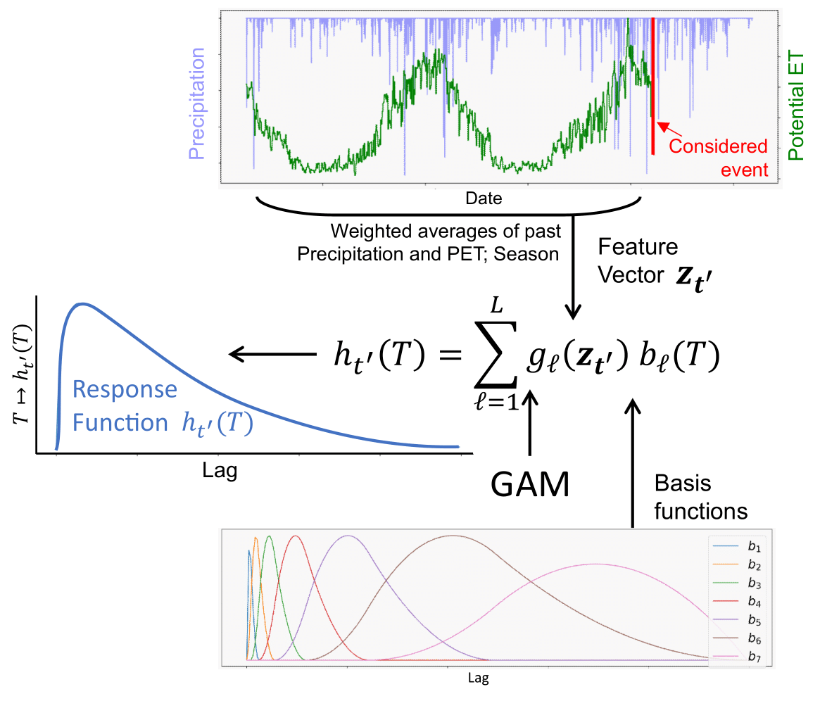
Figure 1 Overview of GAMCR. Given some precipitation event of interest occurring at time t^′, GAMCR computes a feature vector ${\mathit{z}}_{t^{\prime }}$ including information on the system up to time t^′. The response function is expressed as a weighted sum of spline basis functions, (b_ℓ)_ℓ∈[L], where the weights are derived from ${\mathit{z}}_{t^{\prime }}$ through L distinct Generalized Additive Models $\left(g_{\mathrm{\ell }}\right(\cdot ){)}_{\mathrm{\ell }\in \left[L\right]}$.

Since we model the functions ${\left(g_{\mathrm{\ell }}\right)}_{\mathrm{\ell }\in \left[L\right]}$ using GAMs, one can write

$$\begin{array}{}\text{(6)}& g_{\mathrm{\ell }}\left({\mathit{z}}_{t^{\prime }}\right)={\mathit{\xi }}_{t^{\prime }}^{\top }{\mathit{\gamma }}_{\mathrm{\ell }},\end{array}$$

where $({\mathit{\xi }}_{t^{\prime }}^{\top }{)}_{t^{\prime }}$ is the design matrix of the GAM. Each entry of ${\mathit{\xi }}_{t^{\prime }}$ corresponds to one of the spline basis functions evaluated at a given feature (i.e. a specific entry of ${\mathit{z}}_{t^{\prime }}$). We have:

$$\begin{array}{}\text{(7)}& \begin{array}{rl}& y_t=\sum _{\mathrm{\ell }=\mathrm{1}}^L{\left(\sum _{T=\mathrm{0}}^{T_{\max }}{x}_{t^{\prime }}{b}_{\mathrm{\ell }}\left(T\right){\mathit{\xi }}_{t^{\prime }}\right)}^{\top }\\ & {\mathit{\gamma }}_{\mathrm{\ell }}=\sum _{\mathrm{\ell }=\mathrm{1}}^L{\mathbf{W}}_{t,\mathrm{\ell },:}{\mathit{\gamma }}_{\mathrm{\ell }}={\overrightarrow{\mathit{w}}}_t^{\top }\overrightarrow{\mathit{\gamma }},\end{array}\end{array}$$

where $\overrightarrow{\mathit{\gamma }}:=\mathrm{vec}({\mathit{\gamma }}_{\mathrm{\ell }},\mathrm{\ell }\in [L\left]\right)$ and ${\overrightarrow{\mathit{w}}}_t:=\mathrm{vec}({\mathbf{W}}_{t,\mathrm{\ell },:},\mathrm{\ell }\in [L\left]\right)$ given by $\mathbf{W}\in {\mathbb{R}}^{n\times L\times d_s}$ such that:

$$\begin{array}{}\text{(8)}& {\mathbf{W}}_{t,\mathrm{\ell },:}=\sum _{T=\mathrm{0}}^{T_{\max }}{x}_{t^{\prime }}{b}_{\mathrm{\ell }}\left(T\right){\mathit{\xi }}_{t^{\prime }}.\end{array}$$

Here, d_s is the number of features resulting from the GAM formulation.

2.3 Model training

With GAMs we can encode prior knowledge and control overfitting by using penalties and constraints during training. In our case, we consider two smoothness-inducing penalties. The first one promotes the smoothness of the functions g_ℓ by penalizing the second order derivative, as commonly done in the GAM literature (see Hastie et al., 2017). This penalty ensures that the coefficients of the transfer functions in the basis (b_ℓ)_ℓ smoothly evolve with respect to the catchment features ${\mathit{z}}_{t^{\prime }}$. This penalty acts on the L time-dependent coefficients of the transfer functions in the basis (b_ℓ)_ℓ independently. The second regularization term promotes the smoothness of the transfer functions globally by adding a similar penalty on the model coefficients.

The final optimization problem considered is:

$$\begin{array}{}\text{(9)}& \begin{array}{rl}& \underset{({\mathit{\gamma }}_{\mathrm{\ell }}{)}_{\mathrm{\ell }\in \left[L\right]}\ge \mathrm{0}}{min}{\displaystyle \frac{\mathrm{1}}{n}}\sum _{t=\mathrm{1}}^n(y_t-\sum _{\mathrm{\ell }=\mathrm{1}}^L{\mathbf{W}}_{t,\mathrm{\ell },:}{\mathit{\gamma }}_{\mathrm{\ell }}{)}^{\mathrm{2}}\\ & +{\mathit{\lambda }}_{\mathrm{1}}\sum _{\mathrm{\ell }=\mathrm{1}}^L{\mathit{\gamma }}_{\mathrm{\ell }}^{\top }{\mathit{P}}_{\mathrm{1}}{\mathit{\gamma }}_{\mathrm{\ell }}+{\mathit{\lambda }}_{\mathrm{2}}\sum _{\mathrm{1}\le \mathrm{\ell },k\le L}{\displaystyle \frac{\mathrm{1}}{n}}\sum _{t^{\prime }=\mathrm{1}}^n\\ & \left({\mathit{\xi }}_{t^{\prime }}^{\top }{\mathit{\gamma }}_{\mathrm{\ell }}\right)\left[{\mathit{P}}_{\mathbf{2}}{]}_{\mathrm{\ell },k}\right({\mathit{\xi }}_{t^{\prime }}^{\top }{\mathit{\gamma }}_k),\end{array}\end{array}$$

which can be equivalently written using a vectorized formulation as:

$$\begin{array}{}\text{(10)}& \underset{\overrightarrow{\mathit{\gamma }}\ge \mathrm{0}}{min}{\displaystyle \frac{\mathrm{1}}{n}}\sum _{t=\mathrm{1}}^n(y_t-{\overrightarrow{\mathit{w}}}_t^{\top }\overrightarrow{\mathit{\gamma }}{)}^{\mathrm{2}}+{\overrightarrow{\mathit{\gamma }}}^{\top }\left[{\mathit{\lambda }}_{\mathrm{1}}{\mathit{P}}_{\mathrm{1}}^{\prime }+{\mathit{\lambda }}_{\mathrm{2}}{\mathit{P}}_{\mathrm{2}}^{\prime }\right]\overrightarrow{\mathit{\gamma }},\end{array}$$

where, denoting by ⊗ the Kronecker product between two matrices we have defined

$$\begin{array}{}\text{(11)}& {\mathit{P}}_{\mathrm{1}}^{\prime }:={\mathrm{Id}}_L\otimes {\mathit{P}}_{\mathrm{1}},\text{and}{\mathit{P}}_{\mathrm{2}}^{\prime }:={\mathit{P}}_{\mathrm{2}}\otimes \left({\displaystyle \frac{\mathrm{1}}{n}}\sum _{t^{\prime }=\mathrm{1}}^n{\mathit{\xi }}_{t^{\prime }}{\mathit{\xi }}_{t^{\prime }}^{\top }\right)\end{array}$$

Provided that the hyperparameters λ₁ and λ₂ are not both zero, the optimization problem Eq. (10) has a strongly convex objective function with convex constraints. As a result, it admits a unique optimal solution, and the projected gradient descent algorithm is guaranteed to converge to this solution provided that the learning rate is set small enough (cf. Boyd, 2004). For all experiments, we used ${\mathit{\lambda }}_{\mathrm{1}}={\mathrm{10}}^{-\mathrm{3}}$ and λ₂=1 (we refer to Sect. 3.3 for further details). In practice, the parameters $\overrightarrow{\mathit{\gamma }}$ are initialized by solving the unconstrained version of the problem, which involves computing the minimum L²-norm solution via the pseudoinverse of a matrix. This initial solution is then projected onto the positive orthant, after which the projected gradient descent algorithm is applied. The learning rate starts at a large value (namely 10⁻¹) and is gradually and adaptively reduced throughout the iterations to ensure a strict decrease in training loss at each step.

The matrix W is precomputed offline prior to running the projected gradient descent algorithm, and parallel computation can be employed to obtain W quickly. This precomputation significantly accelerates the training process by eliminating redundant calculations.

2.4 Software GAMCR v1.0 description

The model developed in Sect. 2.2 has been implemented in the Python language as the software GAMCR v1.0. The code is publicly available on Zenodo (Duchemin, 2025), and a detailed online tutorial https://quentin-duchemin.github.io/GAMCR/tutorials/ (last access: 30 September 2025) is provided to guide users through usage and reproducibility steps. To use GAMCR, the user must provide time series of precipitation, streamflow, potential evapotranspiration and the corresponding dates and times at equally spaced time intervals. The software operates in a series of steps to ensure accurate and efficient analysis. First, users can use a pre-defined notebook to ensure that their data has the proper format (e.g. column names that conform to the software's requirements). Next, a predefined script is run to perform key precomputations, including the calculation of the matrix W, which significantly enhance the efficiency of the model training process. These precomputations are completed within a few seconds to a few minutes on a standard laptop for a decade of hourly data. Once these precomputations are completed, users can proceed to train the GAMCR model on their dataset. Let us stress once again that the number of basis functions L used by the model is automatically computed based on the maximum lag T_max. With $T_{max}=\mathrm{5}$, 10 or 15 d the model uses 6, 7 or 8 basis functions, respectively. After the model has been trained, users can launch another predefined script to compute key statistics of interest, such as the NRFs over predefined ensembles (such as different precipitation quantiles) and the RRD. These results are automatically saved for further analysis. A detailed tutorial is provided in the online documentation of the GAMCR package, where users can reproduce the results of this paper for the Euthal catchment. The tutorial offers a step-by-step explanation of each stage, equipping users with the necessary tools to apply GAMCR effectively to their own datasets. Overall, GAMCR can be efficiently used on personal laptops, with model training on 20 years of hourly data typically taking around 30 min for $T_{max}=\mathrm{10}$ d.

3 Model testing

Developing strategies to rigorously quantify the performance of trained machine learning models is essential. In the case of the hydrologic response, the evaluation step is particularly important because impulse response functions cannot be measured directly, and the model is trained on streamflow data only (Gupta et al., 2008; McDonnell and Beven, 2014; Kirchner, 2022).

Below, we describe two datasets that serve two different purposes. A synthetic dataset (Sect. 3.1) is used to validate the model, because the estimated response can be compared against the benchmark “ground truth” response, which is exactly known (unlike in real-world catchments). An observed dataset (Sect. 3.2), which includes measurements from six diverse catchments across Switzerland, is used to showcase how the model can be used to estimate the hydrologic response at different locations.

3.1 Synthetic data and model validation strategy

3.1.1 Generation of Synthetic Data

The synthetic dataset was generated using precipitation and air temperature measurements available from the Federal Office of Meteorology and Climatology (MeteoSwiss) for the station of Lugano, along with streamflow data from the nearby gauging station Chiasso, Ponte di Polenta, on the Breggia River. These measurements were used to calibrate a lumped nonlinear and nonstationary conceptual model (Sect. S2), allowing us to create a synthetic streamflow time series (40 years at hourly resolution) that realistically reflects observed dynamics (case A) without aiming for exact replication. To explore different hydrological responses, we adjusted the model parameters to represent both a more damped (case B) and a more flashy (case C) hydrologic system. By working with these synthetic yet realistic datasets, we can rigorously assess the model's performance, because the underlying mechanisms are exactly known and the data are free from disturbances such as dams, hydropeaking, or leakages. Details of the approach employed in the model and the parameters used are provided in Sect. S2.

The generated synthetic time series are shown in Fig. 2 over an example 4-month period. The figure shows clearly that, compared to the reference streamflow series (case A), the damped series (case B) has lower peaks and longer recessions, while the flashy series (case C) has higher peaks and similar recessions. The data also clearly show the nonlinearity and nonstationarity of hydrologic systems, as some precipitation events cause almost no streamflow response (e.g. in June 2010) while others may cause a sharp response (e.g. in late August 2010).

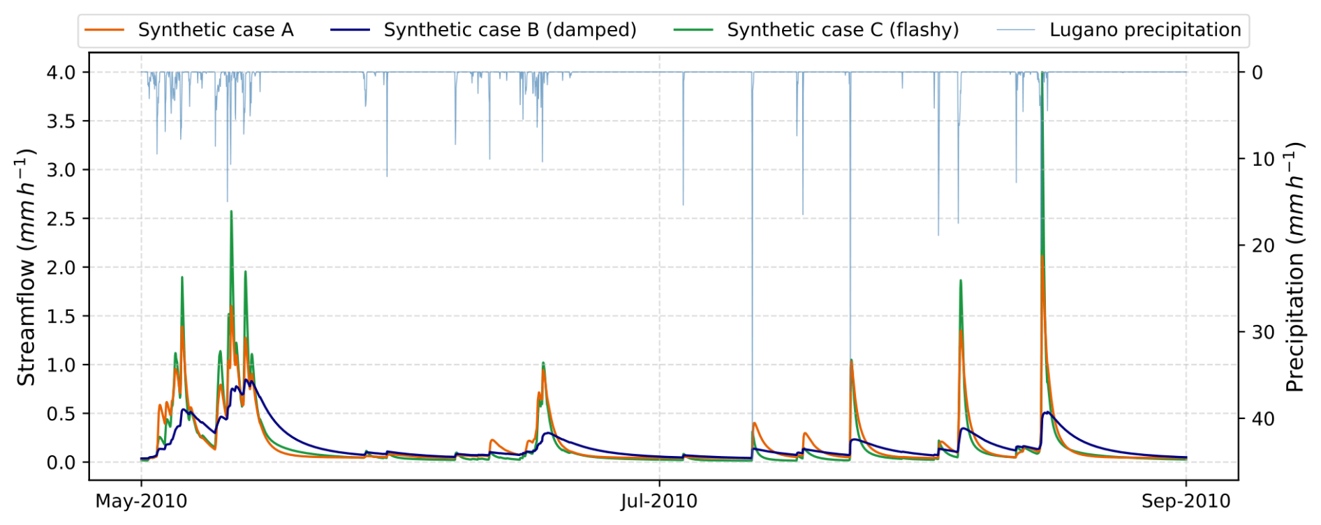
Figure 2 Example of the synthetic streamflow time series (for snow-free months in 2010): case A is the reference (orange curve); case B is a more damped response (purple curve), with lower peaks and longer recessions; case C is a flashier response with higher peaks (green curve). Additionally, the Lugano precipitation time series is shown (light blue curve) with an inverted y axis for comparison.

To compute the response functions for the synthetic data (ground-truth response), we simply ran the lumped hydrological model as many time as there were time steps with nonzero precipitation. In every simulation, we masked a different time step by setting its precipitation to zero. The hydrologic response to precipitation occurring on a specific time step was then computed as the difference between the modeled series with and without precipitation over that time step. This approach provides responses for each event individually, which can be aggregated to compute ensemble responses over e.g. particular periods, precipitation events or antecedent conditions.

3.1.2 Model validation strategy

For each of the three synthetic study cases, GAMCR was trained, and hydrologic responses were computed from the trained model as NRFs aggregated over six precipitation-intensity quantiles. Validation was performed by comparing the GAMCR predictions the corresponding aggregated ground-truth NRFs from the synthetic datasets. We also compared our estimates with those derived from ERRA. Detailed results of the validation are presented in Sect. 4.1.

3.2 Real-world data

We compiled a 15-year record (2005–2019) of measured, hourly precipitation-runoff data from six Swiss watersheds (Fig. 3). The data from the first 13 years were used for model training, while the final two years of data (2018 and 2019) served as the test period. Streamflow time series were provided by the Federal Office for the Environment (FOEN). Precipitation data were sourced from the `CombiPrecip' product, developed by MeteoSwiss (MeteoSwiss CombiPrecip, 2005). Potential evapotranspiration time series were computed based on air temperatures provided by MeteoSwiss, through the Hargreaves method from Hargreaves and Samani (1985) (implemented through the Python Pyeto package https://github.com/woodcrafty/PyETo, last access: 30 September 2025) and then uniformly distributed across each day at hourly intervals. At each site we also extracted key catchment attributes and hydrological statistics (Tables 1 and 2) and computed the mean monthly precipitation, streamflow, potential evapotranspiration over the study period (Fig. 4), and the flow duration curve for the snow-free period (Fig. 5). We selected these sites because of their diversity in hydrological regimes, elevation and soil depths, which we expect will be reflected in substantially different hydrologic responses. Additional criteria included minimal glacier influence, natural flow regimes (no dams or major abstractions), and complete, reliable data records. The sites have comparable size (between 34–185 km²), which classifies them as small to small/medium basins. Further catchment characteristic analyses appear in Sect. S1 in the Supplement.

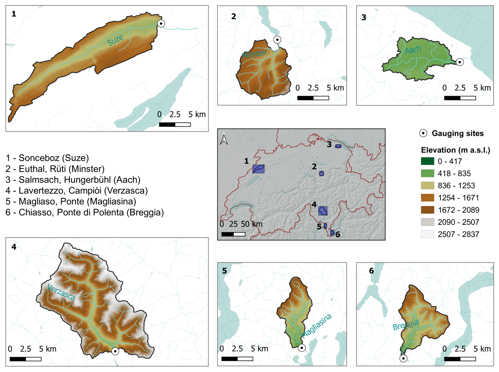
Figure 3 Map of Switzerland showing the six catchments analyzed, along with their corresponding gauging stations (listed on the left with the river names in brackets). Each catchment is displayed in a separate plot for a detailed view of its dimensions and elevation ranges. Numbers mark the catchments' locations within Switzerland and can be seen on the map in the center. The sixth gauging station (Chiasso, Ponte di Polenta) also provided the streamflow time series used to create the synthetic dataset with precipitation data from Lugano.

Table 1 Overview of the gauging stations and their catchment features: associated river; mean elevation; mean slope; area; mean soil depth; mean permeability.

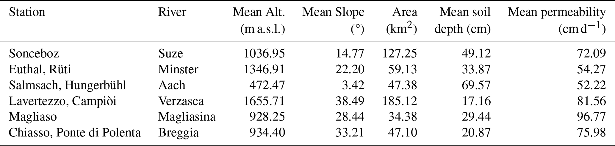
Table 2 Overview of the gauging stations, their hydrological regime type, and key hydrological statistics: snow-free months considered in the study; 10th, 50th, and 90th percentiles of snow-free streamflow (Q10, Q50, Q90); runoff ratio (RR); and center of timing (CT, expressed as the Julian day when 50 % of the snow-free discharge has occurred)

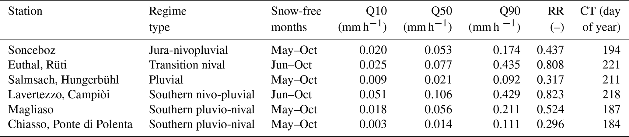
As snow introduces complexities in catchment response, such as delayed runoff generation and temperature-driven melt rates, we focused our analysis on snow-free periods only. We considered as snow-free periods the months from May to October, inclusive, except for two basins at the highest altitudes (Euthal and Lavertezzo, with maximum and mean elevations above 2200 and 1300 m a.s.l., respectively), for which we assumed that first snow-free month is June (Fig. 4).

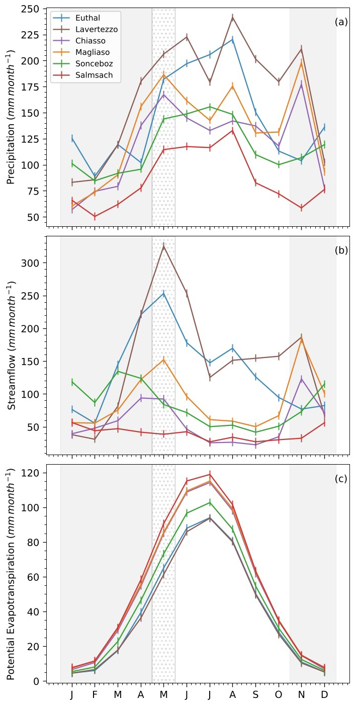
Figure 4 Hydrological regimes, in terms of monthly mean precipitation (a), streamflow (b), and potential evapotranspiration (c) for the six sites. The time series were averaged over the complete period of study (2005–2019). The light grey shadowed areas indicate what we considered as snowy periods with potential snow-melt effects on streamflow, including also May for Lavertezzo and Euthal (dotted grey shadowed band).

Figure 5 shows the Flow Duration Curves (FDCs) of streamflow during the snow-free months. The curves highlight clear contrasts among catchments: Chiasso and Salmsach are dominated by low flows typical of pluvial regimes, while Lavertezzo and Euthal display broader distributions with higher discharges, reflecting steep topography and rapid runoff. Magliaso and Sonceboz fall in between, balancing frequent low flows with moderate events. These patterns confirm that the selected basins capture a meaningful gradient of hydrological responses, even when snow-driven processes are excluded.

Figure 5 Flow Duration Curves (FDCs) for the six sites during the snow-free period (June–October for Euthal and Lavertezzo and May–October for the other basins).

Key hydrological statistics (Table 2) further quantify these differences. Q10–Q90 ranges emphasize the variability between rainfall-dominated and more responsive basins, with Chiasso and Salmsach showing low median flows and narrow ranges, and Lavertezzo and Euthal displaying much higher values. Runoff ratios vary widely (0.30–0.82), while the center of timing (CT) spans from day 184 to 221, marking earlier peaks in pluvial catchments and later ones in higher-elevation sites. Together, these indicators confirm the diversity of regimes and support the suitability of these basins for testing the proposed methodology.

3.3 Implementation details

While our model is designed to estimate the hydrologic response to each precipitation event, we are primarily interested in the model's ability to reproduce the ensemble responses (RRD or NRF) over given conditions of precipitation intensity or antecedent wetness. Therefore, the model will be tested over ensemble responses. This also offers the opportunity to estimate the hydrologic response – and its main statistics – with ERRA and assess the consistency between GAMCR and ERRA.

We tested the need for optimization of the hyperparameters λ₁ and λ₂ through initial (and computationally expensive) cross-validation experiments. Since we obtained only minor improvements over the default values ${\mathit{\lambda }}_{\mathrm{1}}={\mathrm{10}}^{-\mathrm{3}}$, λ₂=1, we consistently used the defaults across all applications. Since we are only interested in the evaluation of the hydrologic response up to a few days after precipitation, we kept the hyperparameter $T_{\max }=\mathrm{24}\times \mathrm{10}$ h. The positions of the knots to get the B-splines basis functions b_ℓ follow an exponentially increasing sequence, starting at 0 with an initial step of 1. After each step, the step size doubles, leading to a pattern where knots are densely spaced at the beginning and become increasingly sparse as values grow. Following this procedure, the value of T_max automatically sets the number of basis functions to L=7 in our case. All models were trained for the full set of predefined epochs using gradient descent with adaptive learning rate, ensuring a strictly decreasing training loss.

In the observed data series, the response to very small rainfall events may be easily hidden by measurement noise and other processes. While these events are not particularly relevant for the hydrologic response, they may corrupt the training phase. Hence it is convenient to set a precipitation intensity threshold J_th and train the model only for events that exceed J_th. We trained GAMCR using J_th=0.05 mm h⁻¹.

The results from ERRA were obtained using the R scripts accessible at the following repository: https://doi.org/10.16904/envidat.529, as specified in Kirchner (2024). The RRD curves were computed considering a maximum lag of 40 h. Initial estimates of precipitation bins were automatically generated by the algorithm, invoking six approximately even ranges, while ensuring a minimum threshold of 40 nonzero values in each precipitation bin. To improve comparability across models, the same precipitation ensembles were used to average the true transfer functions and the GAMCR estimates. Using a coarser input data resolution is beneficial to ERRA when the hydrologic response is long relative to the input temporal resolution (because in such cases, it can be difficult to separate the overprinted effects of input signals at closely spaced lag times). Using a coarser time step helps clarify these impacts. For this reason, after some initial testing, the flashy, base, and damped synthetic input time series are aggregated into 2, 3, and 6 h time steps, respectively.

4 Results

4.1 Model validation

The model was trained (Sect. 2.3) on the synthetic data (Sect. 3.1), which consists of three cases: the reference response, a flashier response, and a more damped response. We validate the model by first computing the hydrologic response in the form of NRF over six quantiles of precipitation intensity, and comparing it against the ERRA estimates and the benchmark generated directly from the model Fig. 6.

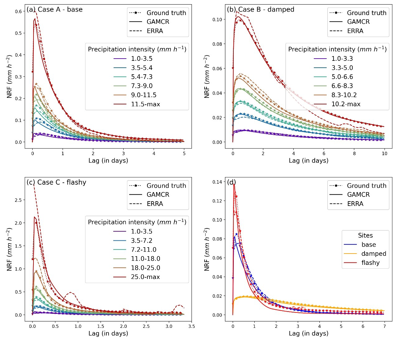
Figure 6 NRFs averaged across different precipitation intensity ensembles from GAMCR, ERRA and the ground truth, for the base (a), damped (b), and flashy (c) synthetic time series. Readers should note the different scales of NRFs between flashy, base and damped scenarios. Panel (d) combines the overall average NRFs for the three cases in a single plot .

As a result of the different aggregation of the input time series for the three synthetic data sets, their precipitation intensities (and thus the bins used in Fig. 6a–c) appear different, although the original hourly input data are the same.

Figure 6 shows that GAMCR accurately estimates the transfer functions on synthetic data, particularly in the flashy and damped scenarios, where their curves nearly overlap with the benchmark. In the base case, (panel a) the peak value and tail of the response are well captured, but the peak timing is systematically early compared to the benchmark. Overall, in these three cases characterized by very different responses (Fig. 6d) ERRA and GAMCR provide generally consistent estimates.

We also computed the peak height, peak lag and runoff volume of the NRF, and explored their relationship with precipitation intensity (Fig. 7). The results highlight GAMCR's ability to accurately estimate key quantities related to the magnitude of the catchment's response (peak height and runoff volume). These statistics are also very consistent with those estimated by ERRA. For both approaches, the flashy case remains the most sensitive for estimation, with GAMCR underestimating runoff volume for intermediate precipitation values (from 10 to 25 mm h⁻¹) but accurately capturing peak height. In the base case, GAMCR slightly underestimates runoff volume while maintaining accurate peak height estimates. For the damped scenario, it closely matches ground truth values for peak height and produces nearly overlapping runoff volume estimates. Overall, both approaches show a strong consistency in their peak height and runoff volume estimates across different scenarios.

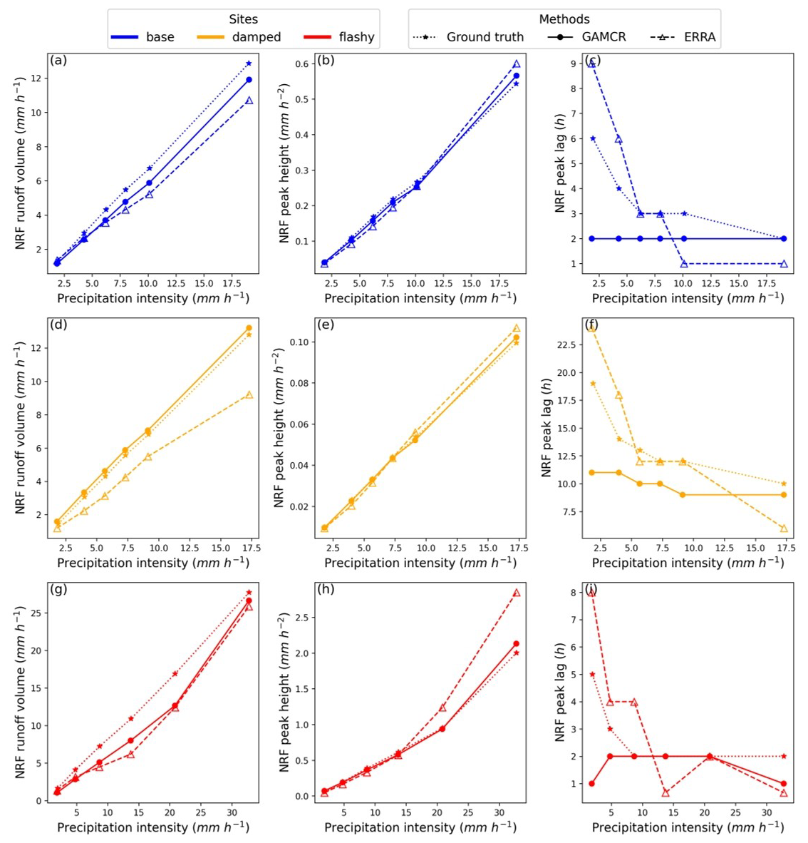
Figure 7 Different statistics computed on NRFs obtained from either GAMCR, ERRA, or the ground truth averaged across different precipitation intensity ensembles for the flashy, base, and damped datasets. Figures (a), (b) and (c) respectively depict the NRF runoff volume, NRF peak height and the peak lag.

Despite the models' strong performance in estimating the magnitude of the catchment response, both face challenges in predicting peak lag, though in opposite ways. ERRA tends to produce more variability across the NRFs (as shown by dashed lines with triangles in all the right panels). By contrast, GAMCR tends to produce lag values that are much less variable than the benchmark across different precipitation ranges.

4.2 Estimation of catchment hydrological responses

When applying GAMCR to observed data it is not possible to validate its accuracy in estimating hydrologic response, because the true response is not known. However, it is instructive to compare the modeled vs measured streamflow series, for both the training and test periods. Since the model was not developed for the purpose of reproducing streamflow, its performance should not be compared to hydrologic models that are designed to maximize fit, but the simulated hydrograph serves as a valuable diagnostic tool. For example, periods where the modeled hydrograph deviates significantly from the measurements could be flagged as unreliable and excluded from the analysis. To support this evaluation, Fig. 8 shows the streamflow predictions generated by GAMCR.

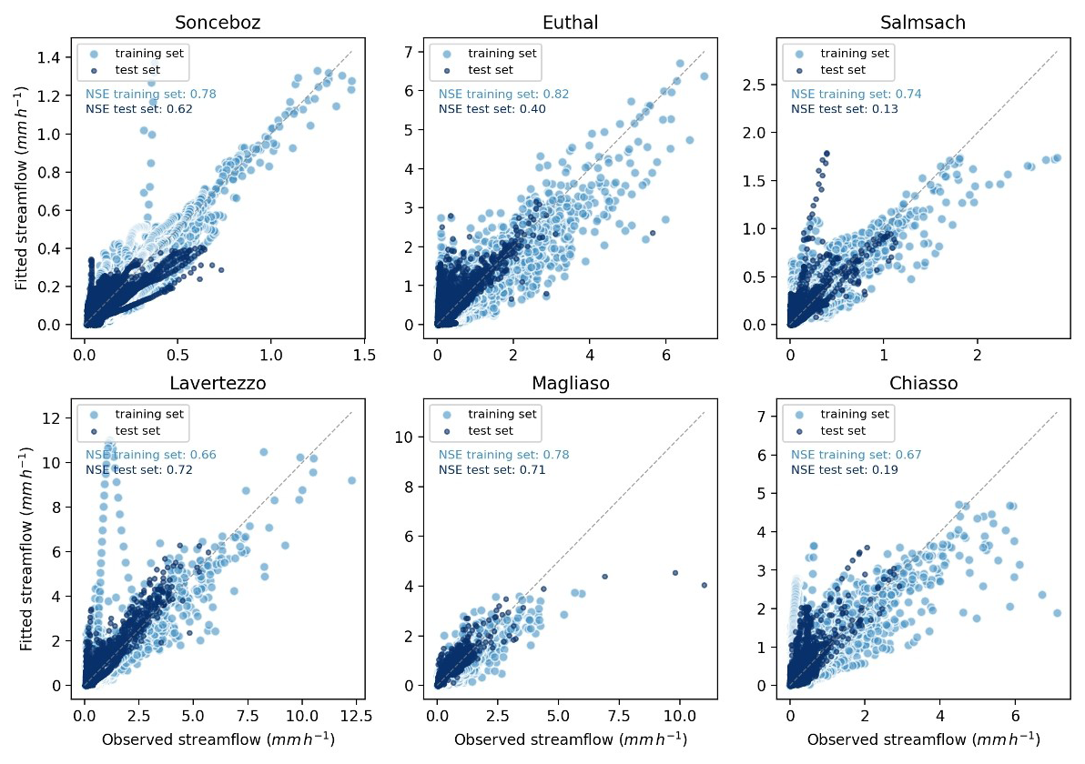
Figure 8 Fitted streamflow estimated through GAMCR for the six investigated sites. The larger light blue dots show measured and fitted discharges during the 2005–2017 snow-free seasons (training set); The smaller dark blue dots indicate measured and predicted discharges during 2018 and 2019 snow-free seasons (test set). 1:1 lines are shown in grey.

The agreement between training and test set results varies across basins. Sonceboz and Magliaso show the strongest consistency, with only minor over- or underestimations. Lavertezzo follows a similar pattern but has some overestimated values on training points. Salmsach and Chiasso, by contrast exhibit considerable dispersion and overestimation on the test set, suggesting lower predictive performance. Performance at Euthal is intermediate between these two groups, with overestimation of low test streamflow values. These results suggest that the performance of GAMCR in reproducing streamflow is not directly correlated with the hydrological characteristics of the basins. This is even more visible when looking at the model performance aggregated over streamflow quantiles (Fig. S2), where the fit is consistently good across sites and only a minor underestimation of the lowest flow conditions stands out. Timeseries plots for the test period (Fig. S3) indicate that the temporal dynamics of the predicted hydrograph are appropriate and there are no periods that should be flagged and removed from the analysis.

Figure 9 presents the weighted average RRDs and the peak heights of the NRFs estimated by ERRA and GAMCR for the six sites in the observed dataset. Computations consider all events whose precipitation intensity exceeds 0.5 mm h⁻¹. The differences in basin response are also evident in the range of runoff coefficients derived from ERRA, which vary from 0.10 in Sonceboz to 0.64 in Euthal. The results align well with the hydrological regimes and characteristics of the basins (see Table 1 and Figs. 3 and 4). The Sonceboz basin, in particular, shows a very flat runoff-response distribution, which is consistent with the relatively low mean slope, large area, and elongated shape of its basin. These features, along with its moderate permeability and location in the Jura's pluvio-nival region, contribute to the basin's very damped runoff response, reflected in the low runoff coefficient (0.10). A slightly flashier response is observed in the Salmsach basin, which has low mean slope, low permeability, and a pluvial hydrological regime. This results in a damped response, though less damped than Sonceboz's, consistent with its higher runoff coefficient (0.19). The Chiasso and Magliaso basins exhibit similar peak values, but with different response shapes. Despite similarities in altitude and mean slope, Chiasso is larger than Magliaso and has lower permeability, consistent with the larger area under its RRD (i.e. the runoff coefficient, 0.26 versus 0.23 for Magliaso). The flashier response in Magliaso is consistent with its high mean slope, in common with Lavertezzo and Euthal, where the flashiest responses (at least for GAMCR) are observed. Lavertezzo and Euthal are characterized by the highest altitudes, highest annual precipitation and lowest annual potential evapotranspiration. The higher RRD peak for Euthal compared to Lavertezzo is consistent with the lower permeability in the Euthal basin and is also reflected in its larger runoff coefficient (0.64 versus 0.40). Overall, the weighted average RRDs provided by both GAMCR and ERRA are broadly consistent with the distinctive characteristics of each basin. The results shown in Fig. 9 demonstrate the general consistency between the GAMCR and ERRA approaches across the different sites. Only two basins exhibit some discrepancy: the Chiasso and Lavertezzo basins (purple and brown curves, respectively). In both these cases, GAMCR estimates a more pronounced RRD peak than ERRA within the first 7 h, and a slightly lower tail after 10 h. The estimated NRF peaks for different precipitation intensities for these sites (Fig. 9d and f) are consistent between ERRA and GAMCR for most precipitation bins, but deviate slightly for the highest one. Overall, the responses estimated by GAMCR and ERRA are broadly similar, and since the models work very differently, consistency in their estimates increases our confidence in both approaches.

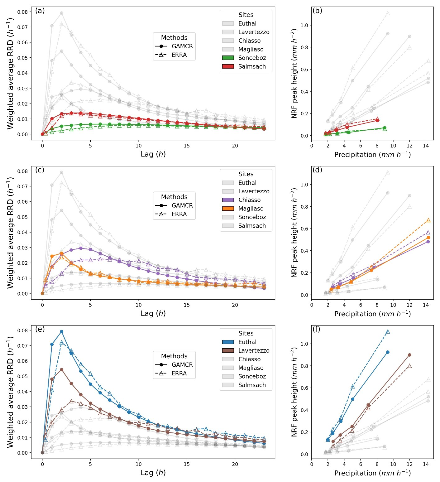
Figure 9 Hydrologic responses and their relationship with precipitation intensity for GAMCR and ERRA. Panels (a), (c) and (e): Weighted average RRD, where we keep time points with precipitation intensity above 0.5 mm h⁻¹. Panel (b), (d) and (f): NRF peak heights against precipitation intensity.

4.3 Effects of precipitation intensity and antecedent wetness

GAMCR can be used to investigate how variations in precipitation intensity and antecedent wetness affect the hydrologic response. Here we explore such effects at the six study sites. To characterize precipitation intensity, we use the same six precipitation intervals defined in Sect. 4.2 above. As a proxy for antecedent wetness, we use the values of streamflow during the timestep prior to the precipitation event under consideration, which we separate into five ranges. We then aggregate the individual response (RRD curves) over each class of precipitation intensity or antecedent wetness. Results are shown in Fig. 10, where we plot the RRD peak height (not to be confused with the peak of the NRF shown in Fig. 9) against precipitation intensity and antecedent wetness.

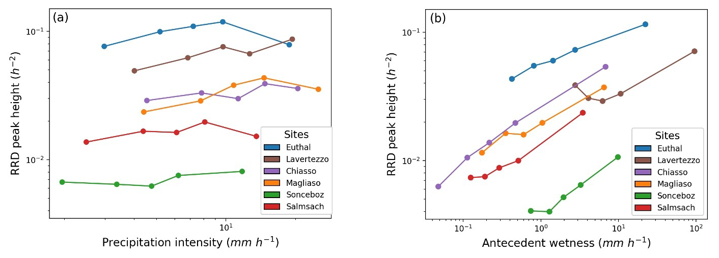
Figure 10 Peak height of RRDs when stratifying with respect to precipitation intensity (a) or antecedent wetness (b).

As Fig. 10a shows, the RRD peak heights do not vary systematically with precipitation intensity. By contrast, Fig. 10b demonstrates clear increasing trends in RRD peak heights with increasing antecedent wetness. Nearly all sites exhibit at least a threefold increase in peak heights across antecedent wetness levels, with the exception of Lavertezzo, which shows a rise in peak heights just for only the last two bins of antecedent wetness. Chiasso, in particular, displays the highest variability, with peak heights spanning almost an order of magnitude (from 0.006 to 0.05 h⁻¹). Notably, for each site, the highest two antecedent wetness levels are widely separated, leading to a marked increase in RRD peak heights. These findings highlight a clear nonstationary response of the six catchments, strongly influenced by their antecedent wetness.

5 Discussion and Conclusions

We introduced a model based on GAMs to estimate the hydrologic response of watersheds based on precipitation-runoff data. The model was validated against three benchmark synthetic datasets and showed excellent agreement with the response curves of the underlying benchmark model, based only on its input and output time series (Fig. 6). While the accurate reproduction of the individual responses goes beyond the scope of the model, the ensemble responses (RRD and NRF curves) proved accurate. Closer inspection of the statistics of the responses (Fig. 7) showed that GAMCR accurately estimated NRF peak height and volume across different precipitation bins. By contrast, the timing of the NRF peak was generally not very accurate, with GAMCR systematically underestimating the peak lag. While this behavior can likely be improved through a different organization of the basis functions that form the core of the response (Sect. 2.2), GAMCR should currently not be used to estimate the timing of the hydrologic response. Comparisons between GAMCR and ERRA highlight that these two models, despite their very different architectures, provide similar hydrologic responses that closely match the (synthetic) ground truth.

Additionally, we analyzed the runoff response during snow-free periods for six Swiss catchments with diverse climatic and physical characteristics (Sect. 4.2). As the hydrologic response of a catchment is not directly measurable, verifying it in physical basins is challenging. Among the diagnostic tools that help build confidence on the results (beyond the benchmark tests of Sect. 4.1), we verified that the modeled streamflow was generally realistic for both training and test data (Fig. 8) and compared GAMCR's RRD and NRF statistics with those obtained from ERRA (Fig. 9). GAMCR produced results that were closely aligned with ERRA and consistent with the properties of the catchments. For example, the Salmsach catchment, with flatter topography and deeper soils than Euthal, had a slower and less marked average response to rainfall. We conclude that GAMCR is a robust tool to study runoff response behavior in catchments. As such, it enables advanced data-based analyses such as quantifying the effects of precipitation intensity and antecedent wetness on the average response peak (Fig. 10).

Since we have often referred to the ERRA approach (Kirchner, 2024) in our analyses, it is worthwhile to clarify the differences and similarities between ERRA and GAMCR. Both methods aim to estimate runoff response to precipitation based on time series data, and they both can quantify nonlinear and nonstationary runoff responses to precipitation. Both methods also implicitly assume that precipitation intensity and catchment conditions are the main controls on the catchment response. However, the two approaches achieve their (common) objective in radically different ways. ERRA fundamentally works on ensemble responses rather than single events. It extracts information from the entire precipitation-runoff time series or from portions of it that are selected to investigate different periods or conditions (provided that each portion has sufficient data). In contrast, GAMCR estimates the hydrologic response to each individual precipitation event using combinations of spline basis functions, with coefficients determined through machine learning techniques (Sect. 2.2–2.3). These individual responses can then be aggregated to ensemble responses. These different starting points result in different ways to run the models. GAMCR is based on a single training phase to estimate all the responses. Then, users can simply aggregate such responses in various ways as a post-processing phase. Instead, ERRA runs instantly but any sub-setting of the time series (for periods or conditions of particular interest, for example) needs to be specified a priori and the code is re-run for each analysis. The way ERRA and GAMCR are parameterized limits the types of transfer functions they can estimate, embedding specific assumptions about their shape. ERRA produces piecewise linear transfer functions, which might take negative values, especially when the water balance in the data is not maintained. In contrast, GAMCR ensures strictly positive transfer functions and promotes smoothness by relying on smooth basis functions. Other minor operational differences between ERRA and GAMCR include the potential need to aggregate the temporal resolution of the data to improve the estimate (ERRA) and the need for potential evapotranspiration series, along with precipitation and runoff (GAMCR, although in the absence of potential evapotranspiration data the user may simply change the default set of features of GAMCR by removing the ones based on PET). Finally, ERRA not only estimates statistics and responses but also quantifies their uncertainty through standard errors. In contrast, GAMCR currently lacks this capability, highlighting the need for future integration of uncertainty quantification.

These first applications of GAMCR to synthetic and observed data help us identify some current model limitations and encourage further model development. While the peak value and area of the aggregated response functions proved accurate, the timing of the response was not, systematically underestimating the peak lag (Fig. 7). Predicting peak lag is statistically challenging because small changes in lag often cause only minor variations in discharge, making estimation difficult. While larger training datasets can help, model architecture – particularly the choice of basis functions – is crucial. GAMCR's reliance on unimodal basis functions (namely B-splines with irregular knots) may introduce ambiguity, as dense placement at short lags can bias peak selection due to identifiability issues. Future work could focus on learning basis functions directly from data under suitable constraints, allowing models to adapt flexibly to watershed characteristics while preserving meaningful inductive biases.

We also stress that while the model simulates the response to every time step with precipitation, it was only evaluated on its capacity to reproduce ensemble behavior and so we do not recommend using it to evaluate individual responses or predict streamflow time series. Additional features that could be implemented in the future include an uncertainty estimation tool capable of providing accurate uncertainty bounds in the response, and the opportunity to integrate additional data (e.g. soil moisture series from sensors or remote sensing products) while training the model.

Catchments' capacity to mobilize water after storm events is a distinctive feature that is relevant for water resources management and useful to characterize catchment behavior. Quantifying the runoff response to precipitation using data-driven approaches is challenging due to the nonlinear and nonstationary nature of streamflow generation processes. GAMCR addresses these challenges by introducing a robust and flexible framework that leverages spline basis functions and Generalized Additive Models to learn the model’s time-variable coefficients. Overall, GAMCR is a modern and effective tool for using the increasingly available rainfall-runoff series to investigate controls on hydrologic responses. Although testing and validation were performed in Swiss catchments, the basins studied span a gradient of physical properties and hydrologic regimes that result in different hydrologic responses. Broader testing of the approach in other climatic regions is a key next step for future research.