Satellite-based modeling of wetland methane emissions on a global scale (SatWetCH4 1.0)

Wetlands are major contributors to global methane emissions. However, their budget and temporal variability remain subject to large uncertainties. This study develops the Satellite-based Wetland CH₄ model (SatWetCH4), which simulates global wetland methane emissions at 0.25° × 0.25° and monthly temporal resolution, relying mainly on remote-sensing products. In particular, a new approach is derived to assess the substrate availability, based on Moderate-Resolution Imaging Spectroradiometer (MODIS) data. The model is calibrated using eddy covariance flux data from 58 sites, allowing for independence from other estimates. At the site level, the model effectively reproduces the magnitude and seasonality of the fluxes in the boreal and temperate regions but shows limitations in capturing the seasonality of tropical sites. Despite its simplicity, the model provides global simulations over decades and produces consistent spatial patterns and seasonal variations comparable to more complex land surface models (LSMs). Such an independent data-driven approach based on remote-sensing products is intended to allow for future studies of intra-annual variations in wetland methane emissions. In addition, our study highlights uncertainties and issues in wetland extent datasets and the need for new seamless satellite-based wetland extent products. In the future, there is potential to integrate this one-step model into atmospheric inversion frameworks, thereby allowing for the optimization of the model parameters using atmospheric methane concentrations as constraints and hopefully better estimates of wetland emissions.

1 Introduction

Article 1.1 of the Ramsar Convention (1971) defines wetlands as “areas of marsh, fen, peatland, or water, whether natural or artificial, permanent or temporary, with water that is static or flowing, fresh, brackish, or salt, including marine water areas the depth of which at low tide does not exceed six meters”. Each wetland exhibits very specific local conditions, such as the water source (ombrotrophic or minerotrophic source) and quantity (groundwater level and soil moisture), vegetation (types and density), and soil properties (pH, carbon content, and microbial communities). These areas harbor a rich biodiversity of flora and fauna and play a significant role in regulating water resources, water purification, and flood prevention (Denny, 1994; Meli et al., 2014).

Wetlands are also a crucial element for climate. On the one hand, waterlogged conditions in wetlands lead to a reduction in the rate of decomposition of soil organic carbon (SOC) and thus to a significant accumulation of carbon, such as in peatlands. This wetland SOC stock has been estimated to be around 520 to 710 PgC worldwide (Poulter et al., 2021). On the other hand, anaerobic conditions favor the production of methane (Torres-Alvarado et al., 2005), a powerful greenhouse gas with a global warming potential of 80 ± 26 over 20 years (Forster et al., 2021, Assessment Report 6 (AR6), Chap. 7, Table 7.15). In the last Global Methane Budget (GMB) (Saunois et al., 2020), it has been estimated that methane emissions from wetlands contribute approximately 12 % to 36 % of the total methane sources. These estimates have been established from bottom-up (102–182 Tg CH₄ yr⁻¹, 12 %–31 % of total annual sources) and top-down approaches (159–200 Tg CH₄ yr⁻¹, 27 %–36 % of total annual sources).

Top-down approaches rely on a prior estimate of the ensemble of methane fluxes, including prior knowledge of wetland emissions, and are therefore dependent on bottom-up estimates. Bottom-up approaches estimate methane fluxes from wetlands using formulations ranging from the simplest to the most complex, such as in land surface models (LSMs). LSMs represent the budgets of water, energy, and carbon under some meteorological constraints. They account for soil processes in a series of successive steps that explicitly simulate part or all of the following processes: methane production; oxidation; and transport by diffusion, ebullition, or higher plants (Riley et al., 2011; Morel et al., 2019; Salmon et al., 2022).

In the context of climate change, understanding past and predicting future trends in global wetland methane emissions are key issues, but these trends are still uncertain (Jackson et al., 2020). Although they try to represent complex pathways involved in methane emissions, LSMs still lead to significant uncertainties in terms of global total emissions, seasonal cycle and spatial patterns (Melton et al., 2013; Saunois et al., 2020). In particular, the internal wetland surface area varies considerably from one LSM to another (Melton et al., 2013). Moreover, a large part of the studies (Zhu et al., 2013; Bohn et al., 2015; Guimberteau et al., 2018; Peltola et al., 2019; Qiu et al., 2019; Salmon et al., 2022; Tenkanen et al., 2021; Kuhn et al., 2021; Rößger et al., 2010) focus only on boreal and temperate regions. In fact, the boreal regions are of great interest because temperatures there are rising faster than the global average (England et al., 2021; Post et al., 2019; Previdi et al., 2021), and permafrost is thawing, which could lead to large increases in carbon dioxide and methane emissions (Schuur et al., 2022). However, about three-quarters of global wetland methane emissions actually occur in tropical regions (Saunois et al., 2020), where wetland methane emissions are still poorly understood (Meng et al., 2015), partly due to the scarcity of measurements in tropical wetlands compared to boreal and temperate regions (Delwiche et al., 2021).

Simpler formulations than LSMs, operating on a global scale (Gedney, 2004; Bloom et al., 2017; Albuhaisi et al., 2023), implicitly represent soil processes in a one-step approach between soil organic carbon content, which is the main substrate for methanogenesis, and CH₄ emissions. While these models may not provide greater accuracy compared to LSMs, they have the advantage of operating faster (within a few seconds) and relying on only a few parameters and variables. They provide quick estimates and can be valuable for sensitivity testing or trend analysis. Typically, the variables considered in the different models are the wetland area, the soil temperature, a proxy for carbon substrate, and sometimes a local water variable (water table depth, WTD, or soil water content, SWC). The differences between these simple models depend on the equation formulation, the choice of datasets used to constrain the variables, and the calibration method.

Methanogenic bacteria use organic carbon from litterfall, root exudates, dead plants, and dissolved organic carbon that has already been broken down to low-molecular-weight molecules by other microorganisms (Nzotungicimpaye et al., 2021; Torres-Alvarado et al., 2005; Bridgham et al., 2013). Quantifying the organic matter available for methanogenesis is not trivial as it cannot be measured directly. Many proxies are used in the literature without a consensus being found (Wania et al., 2013; Melton et al., 2013): Some models use net primary productivity (NPP) as a proxy (e.g., UW-Vic, Walter and Heimann, 2000), while others consider that methane production could be derived by multiplying heterotrophic respiration by a CO₂:CH₄ ratio (e.g., LPJ, CLM4Me, and SDGVM). Other models use SOC as a proxy for carbon available for methanogenesis (Gedney, 2004). However, not all SOC can be used for respiration by methanogenic bacteria. Carbon pool models are embedded in some LSMs such as ORCHIDEE (Ringeval et al., 2010; Salmon et al., 2022) to distinguish readily available SOC from recalcitrant SOC.

In the absence of global data on substrate availability, Gedney (2004) proposed a simple equation based on wetland fraction, temperature, and total soil carbon. These three variables were modeled using the Met Office climate model (Gordon et al., 2000) coupled with the land surface scheme MOSES-LSH (Gedney and Cox, 2003), and their model was run for the period from 1990–1998. Bloom et al. (2017) also used a simplified approach based on an equation relying on wetland fraction, soil temperature, and soil heterotrophic respiration and fed with different datasets, forming the WetCHARTs 1.0 ensemble for 2001–2015. The heterotrophic respiration data were derived by terrestrial biosphere models. In general, the proxies used in these studies are derived from models (LSMs, hydrological models, etc.) and in some rare cases from remote-sensing data. Recently, Albuhaisi et al. (2023) proposed a methane emission formulation fed only by satellite and satellite-derived datasets for soil moisture and SOC. However, this approach was carried out only in the boreal region for the period from 2015–2021.

The calibration methods of these approaches have varied in recent years due to important changes in the available data. The first attempt by Gedney (2004) assumed that the global atmospheric concentration anomalies were solely due to wetlands. This approximation is highly questionable according to current estimates of anthropogenic and natural methane emission trends (Jackson et al., 2020). Too few flux data measurements were available in the early 2000s to be used for calibration. In WetCHARTs (Bloom et al., 2017), the model calibration was performed by constraining total wetland methane emissions to the GMB ensemble mean (Saunois et al., 2016) and as such was not independent of other LSM approaches. However, recent efforts by the FLUXNET community (Delwiche et al., 2021) have led to the construction of a unified database of methane fluxes measured by eddy covariance worldwide, offering the possibility of new independent calibration methods. The eddy covariance method provides stable and continuous in situ flux measurements over relatively large areas (>100 m²) with limited environmental disturbance (Baldocchi et al., 2001; Kumar et al., 2017). The FLUXNET-CH4 database includes some ancillary data such as soil temperature, gross primary productivity, WTD, or SWC, but not for all sites. An important issue is still the inhomogeneous distribution of flux towers across the globe, with sites mainly located in temperate and boreal regions. Albuhaisi et al. (2023) used 12 flux stations available between 2015 and 2018 from the FLUXNET-CH4 database to calibrate the scaling parameter of their boreal emission models, but the two other parameters (Q₁₀ and T₀) were set according to literature values.

In addition to this improvement in available methane flux data, new dynamic estimates of wetland area have emerged since the studies of Gedney (2004) and Bloom et al. (2017). These estimates are based on either satellite observations or hydrological models. The Wetland Area and Dynamics for Methane Modeling (WAD2M) product, published by Zhang et al. (2021a), provides a complete dynamic map of wetlands, including peatlands. It is partly based on satellite data and is widely used in the community, especially for the GMB (Saunois et al., 2020). Xi et al. (2022) produced an ensemble of 28 wetland extent products derived from TOPography-based hydrological MODEL (TOPMODEL), a hydrological model.

Recently, McNicol et al. (2023) developed a random forest framework (UpcH4) to predict CH₄ fluxes based on 43 wetland sites from the FLUXNET-CH4 database. This approach combined with WAD2M wetland surface estimates allowed them to provide independent global data-driven empirical upscaling of wetland CH₄ emissions.

Our study aims to revise the simplified process-based modeling approach for wetland methane emissions proposed by Gedney (2004), taking advantage of recent developments. The objective is to develop a model framework capable of assessing the main features of wetland methane emissions (annual budget, seasonal cycle, and spatial distribution) on a global scale with a resolution of 0.25° × 0.25°, with a focus on methane flux inter-annual variability. The Satellite-based Wetland CH₄ model (SatWetCH4) is based on a data-driven approach, mostly fed with satellite-derived datasets, to allow for fast and easy sensitivity calculations. SatWetCH4 provides an independent estimate and uses in situ eddy covariance data for model calibration. Particular attention has been paid to the proxy for available carbon. As methanogenic activity has been shown to be related to plant productivity (Bridgham et al., 2013), here we use a Moderate-Resolution Imaging Spectroradiometer (MODIS) plant photosynthesis product to derive a C_substrate dataset to assess the organic matter available for methanogenesis, as described in Sect. 2.1. The aim of deriving the C_substrate product is to obtain a carbon product that (1) best represents the carbon available for methanogenesis, (2) is dynamic, (3) is based on satellite data, and (4) is independent of LSMs.

Section 2 presents the materials and methods, including the model, the satellite-based input datasets, and the calibration procedure. Optimization results are presented in Sect. 3.1, followed by a site-level evaluation of the model in Sect. 3.2. The global-scale results for the period from 2003–2020 are presented in Sect. 3.3. Section 4 examines the model's limitations and prospects for improvement given the current state of modeling.

2 Materials and methods

2.1 Model description

We estimate the methane flux using the following formulation similar to that of Gedney (2004):

$$\begin{array}{}\text{(1)}& F_{{\mathrm{CH}}_{\mathrm{4}}}=k{f}_{\mathrm{w}}{C}_{\mathrm{substrate}}{Q}_{\mathrm{10}}(T{)}^{(T-T_{\mathrm{0}})/\mathrm{10}},\end{array}$$

where k is a scaling factor, f_w the wetland fraction of the pixel, C_substrate the carbon content that is available for methanogenesis, and T the soil temperature. Q₁₀(T) depends on $Q_{\mathrm{10}}^{\mathrm{0}}$, the temperature sensitivity of methanogenesis, and T. It is defined by $Q_{\mathrm{10}}\left(T\right)=Q_{\mathrm{10}}^{\mathrm{0}}{}^{T^{\mathrm{0}}/T}$. T⁰ is set to 273.15 K, resulting in low emissions for frozen or near-frozen soils. Consequently, $Q_{\mathrm{10}}^{\mathrm{0}}$ and k are the two parameters to be calibrated.

The substrate available in the soil for methanogenesis, C_substrate, is calculated independently, upstream of the model. It is constructed as a litter pool model scheme and depends on temperature and net primary productivity (NPP) and varies with time. This C_substrate is computed using the following equation:

$$\begin{array}{}\text{(2)}& {\displaystyle \frac{\mathrm{d}{C}_{\mathrm{substrate}}}{\mathrm{d}t}}=\mathrm{NPP}-K\left(T\right)C_{\mathrm{substrate}}.\end{array}$$

In this scheme, the available substrate is assumed to originate mainly from photosynthesis, which is approximated as the NPP. The second term represents the carbon loss due to soil heterotrophic respiration, which depends on a turnover rate function $K\left(T\right)=K^{\mathrm{ref}}{Q}_{\mathrm{10}K}^{(T-T_K^{\mathrm{ref}})/\mathrm{10}}$. K^ref reflects the reference turnover time, Q_10 K the temperature sensitivity coefficient of respiration, and $T_K^{\mathrm{ref}}$ the reference temperature. Incubation experiments (Parton et al., 1987; Khvorostyanov et al., 2008; Schädel et al., 2014) provided estimates of K between 0.2 and 2.5 yr⁻¹, corresponding to a residence time of carbon in soils between 0.4 and 5.5 years. Therefore, to obtain a consistent K, the model parameters are set to $K^{\mathrm{ref}}=\mathrm{1}/\left(\mathrm{2}\mathrm{years}\right)=\mathrm{0.5}{\mathrm{yr}}^{-\mathrm{1}}$, $T_K^{\mathrm{ref}}=\mathrm{303.15}$ K, and Q_10 K=2.

The global estimate of C_substrate is established in advance by discretizing Eq. (2) at monthly time steps. The C_substrate was primarily run for 100 years to reach an equilibrium stage, constrained with 2001 NPP values obtained from remote-sensing data (Zhang et al., 2017) detailed in Sect. 2.3. NPP data between 2003 and 2020 were then used to estimate C_substrate over the same period on a monthly scale.

2.2 In situ data

Eddy covariance time series of methane fluxes from different databases were combined in order to use robust, continuous, and longest methane flux monitoring period recorded at each site. In situ data from 58 wetland sites were collected from FLUXNET-CH4 (Delwiche et al., 2021), AmeriFlux (Baldocchi et al., 2001), and EURO FLUX (Valentini, 2003). In addition, data for the BW-Gum and BW-Nxr sites were obtained from the UK Centre for Ecology & Hydrology website, and IN-Pic data were provided through personal exchanges with the principal investigator, Palingamoorthy Gnanamoorthy. Some ancillary variables of interest for methane emission modeling (e.g., soil temperatures, WTD, SWC, and precipitation) are available at some of the sites. Links to the sources used are given in Table S1 in the Supplement, and the full list of sites and details is given in Table S2 in the Supplement.

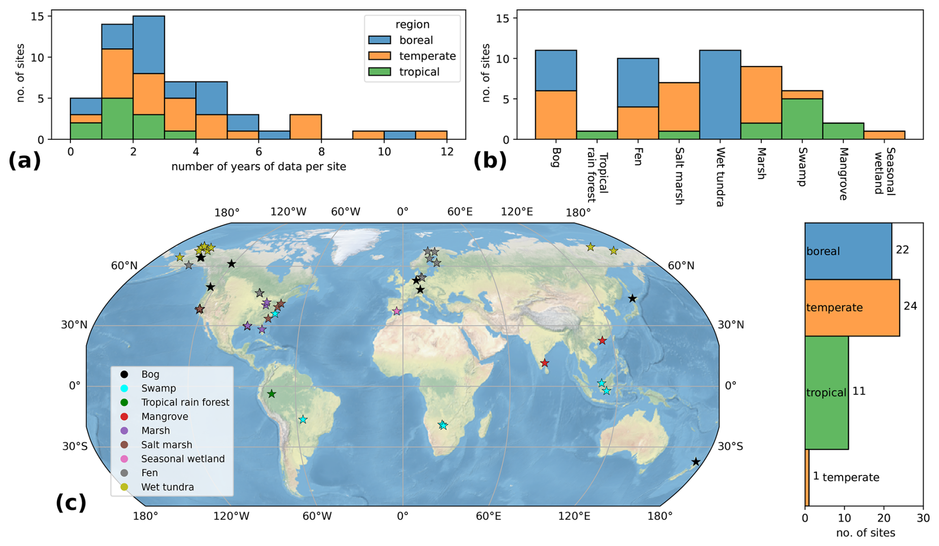
Figure 1 Sites distribution per (a) length of available observation period, (b) wetland type, and (c) geographic location. In the map in panel (c), because of their close location (a few kilometers), some sites overlap. Site color depends on (a, b) site latitude – boreal (55–90° N), temperate (30–55° N or ° S), or tropical (30° S–30° N) – and (c) wetland type.

The length of the time series, wetland types, and location of the sites are presented in Fig. 1. Despite the construction of the most comprehensive database from recent literature, the global distribution of methane eddy covariance tower sites shows significant heterogeneity. The majority of sites, that is, 46 of them, are located at latitudes greater than 30° N, with 36 sites in North America and 10 sites in Europe. Only 11 sites (19 %) are located in the tropical band, 30° S–30° N, including, for example, only 2 sites on the entire African continent, which are only a few kilometers apart, and 2 sites in South America. In addition, Fig. 1a highlights the heterogeneity in measurement duration, with tropical sites having a median measurement duration of 1.6 years, as contrasted with 2.7 and 3.2 years for boreal and temperate sites, respectively. It is also important to note that sites can be very close to each other (within a few kilometers). This uneven distribution of sites introduces a bias in the global calibration of the model. In particular, tropical wetlands are severely underrepresented, although they are expected to account for about ∼ 75 % of global wetland methane emissions (Saunois et al., 2020).

To ensure a homogeneous dataset, the same data processing was applied to the raw data. The 30 min raw data points were extracted, and the variable units were unified. Outliers are removed for all variables, including ancillary data, notably for methane fluxes, for each site and day, data outside of ${\stackrel{\mathrm{‾}}{F_{{\mathrm{CH}}_{\mathrm{4}}}}}_{\mathrm{day}}\pm \mathrm{5}{\mathrm{SD}}_{F_{{\mathrm{CH}}_{\mathrm{4}}}}$_day are excluded. Finally, daily averages are calculated for all variables, and monthly averages are only calculated if more than 4 d of data are available in a given month. A monthly timescale was chosen for this study because it effectively captures seasonal variations while minimizing the influence of variables that operate at shorter time intervals, such as daily or multi-day changes in atmospheric pressure or diurnal cycles in vegetation and temperature (Knox et al., 2021). Furthermore, as our model is a one-step model without differentiation between production and emissions, the monthly timescale also mitigates potential errors due to time lags between methane production and transport (Ueyama et al., 2023).

This results in a dataset of 2354 monthly mean methane fluxes associated with their available ancillary data.

2.3 Global forcing datasets

2.3.1 MODIS PsnNet data

To derive C_substrate estimates, as defined in Eq. (2) in Sect. 2.1, we use PsnNet from the MODIS MOD17A2HGF v6.1 dataset (Running et al., 2021). The PsnNet dataset represents NPP, except that it excludes growth and maintenance respiration costs. This product is based on the satellite fraction of photosynthetically active radiation (FPAR) data, a reanalysis meteorological dataset, and a land cover classification.

The data cover the period from 2000 to the current year, but data for 2002 are not available, so only the period from 2003 to 2020 has been used in this study. The PsnNet product has been regridded from the native 500 m resolution to a 0.05° product used for model optimization at the site level and to a 0.25° resolution product used for the global simulation. In terms of the timescale, monthly averages were estimated from the initial 8 d product.

2.3.2 ERA5-Land soil temperature

For the soil temperature variable, monthly averaged data from ERA5-Land (Muñoz-Sabater et al., 2021), available at https://cds.climate.copernicus.eu/ (last access: 10 January 2023​​​​​​​), are used. The temperature in the 7–28 cm soil layer is selected, denoted as lay2. These data are available for the period from 1950 to the present with a resolution of 0.1° × 0.1°. A comparison of in situ soil temperature measurements with the monthly ERA5-Land lay2 closest 0.1° pixel is detailed in Fig. S2 in the Supplement, showing good agreement between in situ and ERA5-Land soil temperatures, with, in particular, a high temporal correlation (r>0.9) and low root mean square deviation (RMSD; <2 K) for 37 of the 42 sites equipped with temperature probes.

2.3.3 Global wetland extent datasets

Two wetland areas are used to estimate global methane emissions. The Wetland Area and Dynamics for Methane Modeling (WAD2M) version 2.0 (Zhang et al., 2021a) product describes the fraction of wetlands per pixel globally at a resolution of 0.25° × 0.25° for the period from 2000–2018 with a monthly time step. The dynamics of WAD2M are driven by the Surface Water Microwave Product Series (SWAMPS) (Jensen and Mcdonald, 2019), which relies on passive and active microwave satellite observations. Several static datasets are used to add non-inundated wetlands, such as peatlands, and to remove lakes, irrigated rice paddies (Zhang et al., 2021b). The second wetland map used is based on the TOPography-based hydrological MODEL (TOPMODEL). Xi et al. (2022) built an ensemble of 28 maps describing globally the fraction of wetlands per pixel at a resolution of 0.25° × 0.25° for the period from 1980–2020 at a monthly time step (Xi et al., 2021). A combination of seven different soil moisture reanalysis datasets and four different surface wetland extent products was used to calibrate the model. Among the 28 products, we select here the version calibrated with ERA5-Land soil moisture data and the GIEMS-2 (Prigent et al., 2020) long-term maximum as it shows the highest correlations of wetland area with the original wetland product (Xi et al., 2022).

2.4 Calibration method

The in situ methane fluxes at the sites were used to calibrate the SatWetCH4 model parameters k and $Q_{\mathrm{10}}^{\mathrm{0}}$. Model calibration at the site level implies that each site is considered to be completely covered by wetland, resulting in a wetland fraction of 1 (f_w=1). The flux equation to be optimized at site level is then $F_{{\mathrm{CH}}_{\mathrm{4}}}=k{C}_{\mathrm{substrate}}{Q}_{\mathrm{10}}(T{)}^{(T-T_{\mathrm{0}})/\mathrm{10}}$. The C_substrate product (described in Sect. 2.1) and ERA5-Land soil temperature (described in Sect. 2.3) are used as input variables by selecting the pixels nearest to the sites, at 0.05° for C_substrate and 0.1° for ERA5-Land soil temperature, respectively.

Least-squares regression is performed simultaneously on all sites using the Broyden–Fletcher–Goldfarb–Shanno algorithm (Byrd et al., 1995). For sites with less than 12 months of data, a weight proportional to the number of monthly measurements is assigned to the site data. Sites with more than 12 months of data are given equal weights. The minimized cost function is

$$\begin{array}{}\text{(3)}& J=\sum _{\mathrm{sites}}{w}_{\mathrm{site}}{\mathrm{MSD}}_{\mathrm{site}}=\sum _{\mathrm{sites}}{w}_{\mathrm{site}}\stackrel{\mathrm{‾}}{(F_{{\mathrm{CH}}_{\mathrm{4}}\mathrm{obs}}-F_{{\mathrm{CH}}_{\mathrm{4}}\mathrm{sim}}{)}_{\mathrm{site}}^{\mathrm{2}}},\end{array}$$

where w_site is the site weight, MSD is the mean square deviation, $F_{{\mathrm{CH}}_{\mathrm{4}}\mathrm{obs}}$ is the in situ methane flux observed at the sites, and $F_{{\mathrm{CH}}_{\mathrm{4}}\mathrm{sim}}$ is the methane fluxes simulated by the model. If the number of monthly methane flux measurements at the site, n_site, is greater than or equal to 12, w_site=1; otherwise $w_{\mathrm{site}}=\frac{n_{\mathrm{site}}}{\mathrm{12}}$. Different initial parameter sets for k_{first guess} (0.01, 0.1, 1, and 10) and $Q_{\mathrm{10}}^{\mathrm{0}}$_{first guess} (1.5, 2.5, 3, and 4) are tested to evaluate the influence of the calibration initialization and to ensure the global nature of the found minimum.

3 Results

3.1 Optimized model parameters

The calibration is performed according to the method described in Sect. 2.4. The minimum cost function is found for $Q_{\mathrm{10},\mathrm{opt}}^{\mathrm{0}}=\mathrm{2.99}$ and $k_{\mathrm{opt}}=\mathrm{3.097}\times {\mathrm{10}}^{-\mathrm{2}}$ µg CH₄ m⁻² s⁻¹. The value of k_opt has no numerical meaning as it is highly dependent on the units and order of magnitude of the substrate proxy we use. The Q₁₀(T) formulation obtained from this calibration is compared with the literature values in Fig. 2a. Figure 2b shows the influence of Q₁₀(T) expressions when inserted in the temperature formulation $Q_{\mathrm{10}}(T{)}^{(T-T_{\mathrm{0}})/\mathrm{10}}$.

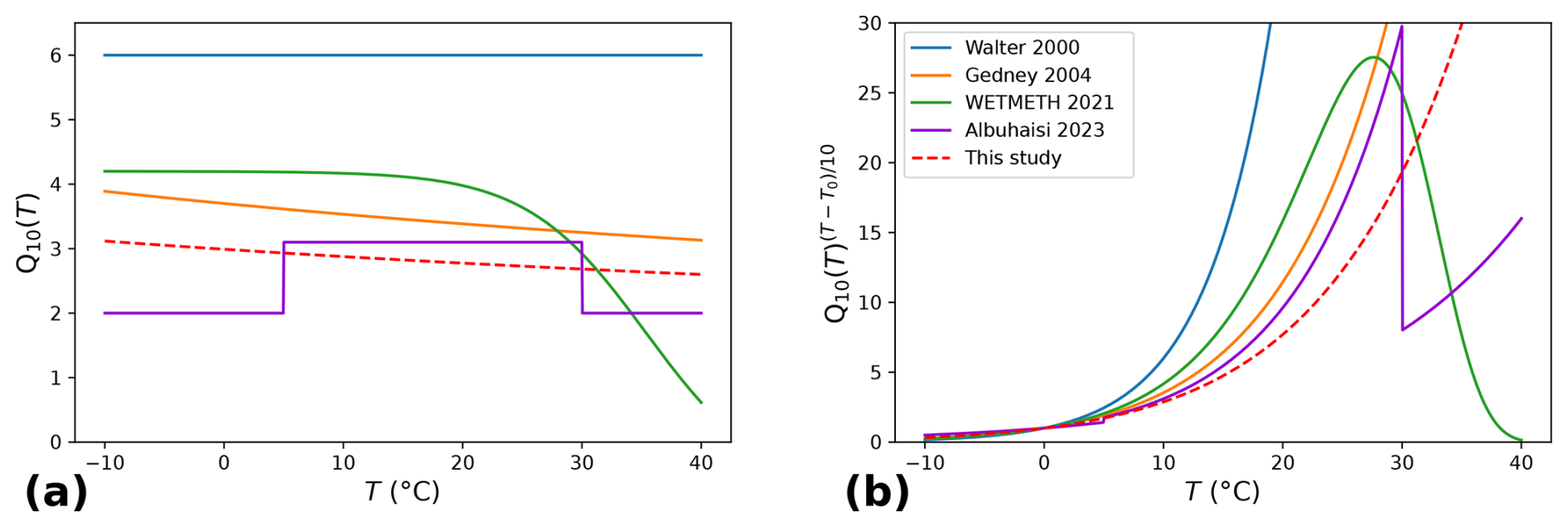
Figure 2 (a) Comparison of Q₁₀(T) formulation with Walter and Heimann (2000), Gedney (2004), WETMETH (Nzotungicimpaye et al., 2021), and Albuhaisi et al. (2023). (b) Effect of the different Q₁₀(T) formulations when incorporated in the temperature dependency function.

Walter and Heimann (2000) used a Q₁₀ value of 6 based on the observations range available at the time. Nzotungicimpaye et al. (2021) in WETMETH proposed a Q₁₀(T) formulation such that, when incorporated into the variable $Q_{\mathrm{10}}(T{)}^{(T-T_{\mathrm{0}})/\mathrm{10}}$, it indicates an optimal temperature range for methanogenesis of around 25–30 °C. Although we attempted a similar approach to formulate Q₁₀(T), it resulted in minimal changes in the flux outcomes while increasing the complexity of the formulation and hindering the convergence of the cost function. Albuhaisi et al. (2023) used a fixed value of Q₁₀ = 3, with a value reduced to Q₁₀=2 for temperatures above 5 °C or above 30 °C to account for an optimal range. However, this results in abrupt transitions at these temperature thresholds (Fig. 2.b). This implementation may not be appropriate for global analysis as tropical wetlands experience temperatures above 30 °C, and such sudden changes do not reflect of physical reality.

Therefore, the Gedney (2004) formulation, $Q_{\mathrm{10}}\left(T\right)={Q_{\mathrm{10},\mathrm{opt}}^{\mathrm{0}}}^{T_{\mathrm{0}}/T}$, was used in SatWetCH4, resulting in Q₁₀(T) from 3.12 (−10 °C) to 2.60 (40 °C), which is slightly lower than the Gedney (2004) value (from 3.89 at −10 °C to 3.13 at 40 °C). Our Q₁₀(T) value contrasts that of Walter and Heimann (2000) (Q₁₀=6.0, no temperature dependence) but closely matches the value chosen by Albuhaisi et al. (2023) for the 5–30 °C range (Q₁₀=3.1 for T between 5 and 30 °C and Q₁₀=2.0 below 5 °C or above 30 °C). Consequently, similar $Q_{\mathrm{10}}(T{)}^{(T-T_{\mathrm{0}})/\mathrm{10}}$ curves are observed in Fig. 2b between our estimate and those of Gedney (2004) and the 5–30 °C range of Albuhaisi et al. (2023), although our formulation exhibits slightly lower values. This would result in a slightly lower increase in methane fluxes with soil temperature. The Q₁₀(T) found in this study is also in agreement with the meta analysis of Q₁₀ defined from in situ data, e.g., 2.8 in Kuhn et al. (2021) and 2.57 in Delwiche et al. (2021).

3.2 Evaluation of the model performance at site scale

To evaluate the SatWetCH4 model, we run it at the site scale with the optimized parameters, setting f_w=1 in Eq. (1) and using the variables values from the pixels closest to the site, i.e., at 0.05° for C_substrate and at a 0.1° resolution for ERA5-Land temperature (resulting monthly estimates can be found in Fig. S1 in the Supplement). Note that the difference in spatial resolution between the site level, i.e., the footprint of the flux towers (up to 1 km²), and the resolution of the available substrate (0.05° × 0.05° ≈ 25 km²) limits the comparison. The temperature is more homogeneous, and its aggregation at 0.1° is less problematic. Figure 3 compares the in situ flux data with the modeled site-level output. Figure 3a shows the root mean square deviation (RMSD) and the temporal correlation (r) between the observations and the simulated flux. It indicates a generally lower average RMSD in the boreal zones (average RMSD of 0.23 µg CH₄ s⁻¹ m⁻²) compared to the temperate zones (average RMSD of 0.8 µg CH₄ s⁻¹ m⁻²) and the tropics (average RMSD of 1.1 µg CH₄ s⁻¹ m⁻²). It shows that the model captures the seasonality of emissions well for boreal sites (r>0.7 for 16 out of 22 boreal sites), less well for temperate sites (r>0.7 for 11 out of 25 sites), and poorly for tropical sites (r>0.7 for 4 out of 11 sites, with 5 out of 11 sites having r<0). Figure 3b and c display the amplitude variations (standard deviation) and mean values of the observed and modeled fluxes. The mean fluxes are consistent with the in situ values (Fig. 3c), while the standard deviation (SD), which represents the amplitude of the seasonal variation, is underestimated for fluxes with an SD greater than 1 µg CH₄ s⁻¹ m⁻² (Fig. 3b).

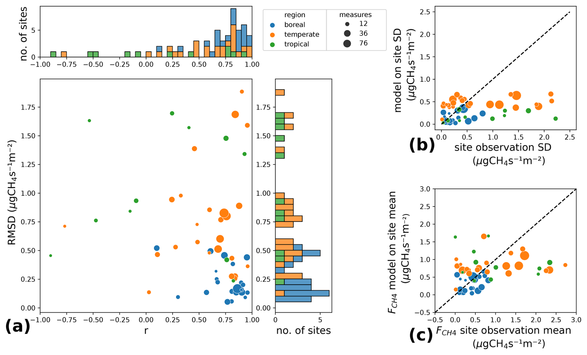
Figure 3 Comparison of methane fluxes modeled at site level with observations. Each site is represented by a point and its location by a different color, while the site number of measurements is represented by point sizes. (a) Temporal correlation (r) and RMSD between the model and observations. (b) The standard deviation (SD) of model fluxes functioning as the standard deviation of observations. (c) Average model fluxes versus average flux observations.

Thus, the model reproduces boreal fluxes better than temperate and tropical fluxes. This results in higher RMSD values for tropical and temperate zones, as shown in Fig. 3a., although these higher RMSD values are also due to generally larger fluxes in the tropics. The underestimation of fluxes in the tropics is partly due to the sampling bias mentioned in Sect. 2.2: only a small proportion (19 %) of the sites are located between 30° S and 30° N, and they have shorter monitoring periods, resulting in a cumulative weight of 18.5 % in the cost function, J (boreal sites weight 38 % and temperate sites 43 %). Furthermore, the mechanisms driving the temporal variations in tropical methane flux are certainly poorly represented in the model, as discussed in Sect. 4.

3.3 Methane emissions from wetlands on a global scale

After calibrating k_opt and $Q_{\mathrm{10},\mathrm{opt}}^{\mathrm{0}}$, we run the SatWetCH4 model (Eq. 1) on a global scale for the period from 2003–2020 at a resolution of 0.25° × 0.25° with forcing dataset C_substrate, ERA5-Land soil temperature, and either the WAD2M or the TOPMODEL product for wetland extent at the same resolution. In the following, we compare the wetland emissions derived from SatWetCH4 in terms of total global methane emissions, spatial distribution, and temporal variations with Bloom et al. (2017), UpCH4 (McNicol et al., 2023), and ensemble mean of the GMB (Saunois et al., 2020).

3.3.1 Comparison of the spatial distribution of the wetland extents

For both products, the monthly average of surface extent served to derive a mean annual mean (MAmean) and mean annual maximum (MAmax) by selecting for each 0.25° pixel the mean or maximum of the typical 12-month seasonality. The maps of MAmean of both wetland extent products are presented in Fig. 4. WAD2M has a global MAmean of 4.21 million km² (Mkm²) and a MAmax of 6.76 Mkm² over 2003–2020, while TOPMODEL is lower at 3.04 and 5.12 Mkm², respectively.

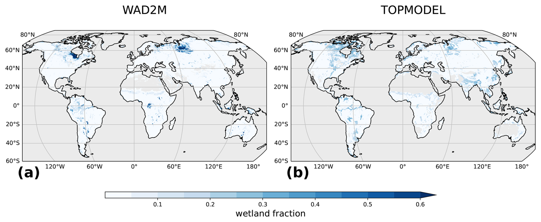
Figure 4 Wetland fraction 2003–2020 annual mean of (a) WAD2M and (b) the model TOPMODEL.

This discrepancy in the value of the total area is mainly due to the methodology employed to construct the products. First, WAD2M is known to overestimate coastal areas due to ocean contamination by nearby ocean pixels in the original SWAMPS data (Pham-Duc et al., 2017; Bernard et al., 2024a). Second, WAD2M includes non-inundated wetlands, such as peatlands, whereas TOPMODEL represents only inundated wetlands. Indeed, Xu et al. (2018) estimate that peatlands cover around 4.23 Mkm². In fact, the WAD2M wetland fraction over peatland areas (e.g., Hudson Bay, the Congo, Siberian lowlands, and Amazon floodplain) is larger than in TOPMODEL (Fig. 4). Note that some boreal peatlands in WAD2M are masked by snow cover in winter, which explains the lower MAmean than the global peatland extent. There are other large spatial differences between the two datasets. Of concern in WAD2M is the substantial detection of water over Australia, a predominantly desert and semi-arid region, and subequatorial Africa (Sahel). Wetlands and deserts have similar microwave signatures, explaining the possible confusion (Pham-Duc et al., 2017). Finally, TOPMODEL shows higher scattered extents over North America, India, and China than WAD2M.

3.3.2 C_substrate spatial distribution

The 2003–2020 mean map of the C_substrate product is shown in Fig. 5. This product is used as a representation of the soil carbon substrate available for methanogenesis. It should be noted that there are no analogous products for evaluation. We suggest a comparison with global estimates of 0–100 cm SOC stocks derived from the World Soil Database (HWSD) (Wieder, 2014) and SoilGrids (Hengl et al., 2017) to see differences between our proxy for available substrate compared to total organic carbon stocks. The latitudinal distribution and the latitudinal distribution normalized by the latitudinal maximum of the three products are shown on the right side of the figure.

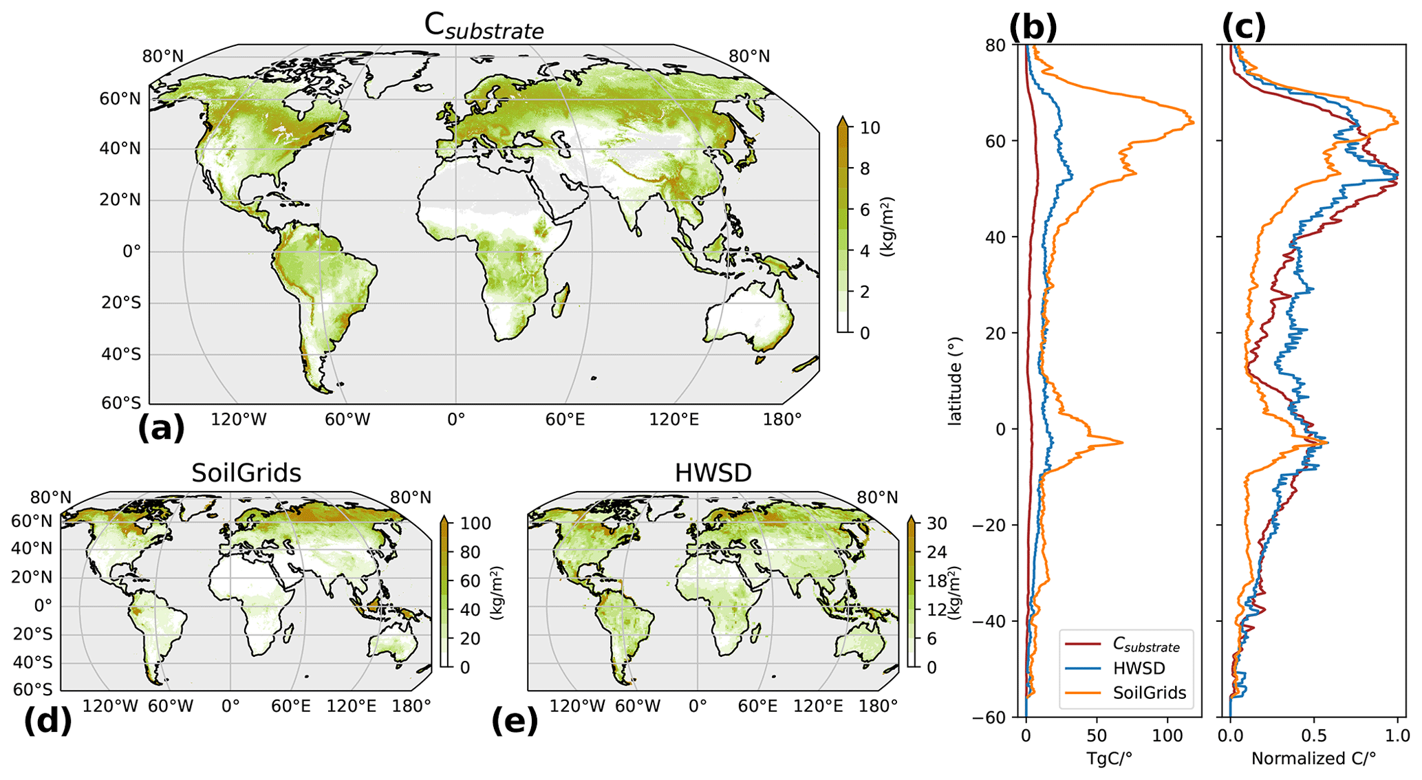
Figure 5 Derived C_substrate product (a) and the 2003–2020 mean alongside two SOC databases (d, e) for the 0–100 cm layer: HWSD (Wieder, 2014) and SoilGrids (Hengl et al., 2017). The corresponding latitudinal and normalized latitudinal profiles are displayed in panels (b) and (c). Normalization is achieved by dividing by the latitudinal maximum for each product.

The numerical values of C_substrate tend to be consistently lower than those of the SOC estimates, differing by about an order of magnitude. This observation aligns with the fact that elevated SOC values, which are particularly common in peatlands, do not translate to a proportionally increased production of CO₂ or CH₄ emissions. In fact, the slow decomposition of organic matter in peatlands leads to carbon sequestration in soils over millennia (Clymo et al., 1998). It is important to emphasize that the order of magnitude of the numerical value of C_substrate is of limited significance since the calibration of the k factor is used for the methane flux calculation. The critical focus is on the spatial variations and temporal dynamics of C_substrate for accurate methane flux assessments.

The C_substrate product shows a small seasonal variation (about 5 % on global and basin scales), implying that its contribution is mainly of spatial nature. Indeed, we observe a different spatial distribution between the three products. SoilGrids and HSWD tend to show more localized high carbon values in regions where peatlands are abundant, such as in the western Siberian lowlands or the northern part of America, or, for SoilGrids, in Indonesia. C_substrate presents a more homogeneous distribution, with moderate values in boreal and temperate regions. It consistently shows no or low available substrate values over bare soil regions (Sahara, Australia). In light of these considerations, C_substrate appears to be a valuable candidate for estimating soil carbon availability.

3.3.3 Spatial variations in methane emissions

The methane fluxes derived from SatWetCH4 are strongly influenced by the spatial patterns of the wetland extent used: the differences between WAD2M and TOPMODEL mentioned in Sect. 3.3.1 are partly reflected in the output fluxes (Fig. 6a and b). In fact, the parameter f_w is directly a multiplicative coefficient in the flux calculation in Eq. (1). In particular, peatland regions emit more in the WAD2M version, and the Ganges and Yangtze basins show much more intense methane emissions when TOPMODEL is used.

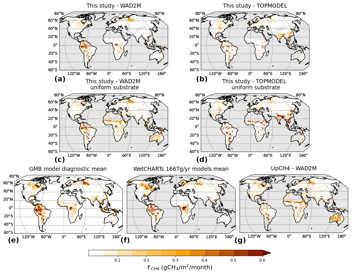
Figure 6 SatWetCH4 modeled mean methane emissions (a) using WAD2M and (b) TOPMODEL wetland surfaces and with a uniform substrate (i.e., C_substrate = 1) (c) using WAD2M and (d) using TOPMODEL. Emissions obtained by (e) the mean of GMB diagnostic models, (f) the mean of WetCHARTs ensemble, and (g) the UpCH4 upscaling.

We assess the sensitivity of SatWetCH4 model to the C_substrate product derived from the NPP (Eq. 2) by comparing the results from a SatWetCH4 reference run (with C_substrate) and a run that considers a uniform substrate (C_substrate=1 over the globe). Note that to do this, we had to calibrate the model parameters k and $Q_{\mathrm{10}}^{\mathrm{0}}$ using the same method described in Sect. 2.4, resulting in a lower $Q_{\mathrm{10},\mathrm{opt}}^{\mathrm{0}}$ (1.83 instead of 2.99). The spatial distribution is then very different (Fig. 6c and d), depending only on the wetland extent dataset and weighted by temperature. In particular, emissions are significantly higher in subequatorial Africa (Sahel) with both wetland datasets when no substrate product is included in the model. In fact, C_substrate is small over this region due to a small value of the MODIS PsnNet input (Fig. 5). Over Australia, we observe significantly higher fluxes with WAD2M when C_substrate is not considered. This shows an overestimation of WAD2M wetland detection in the Australian desert, which is mitigated by the small C_substrate over this region when C_substrate is considered instead of the uniform substrate (Fig. 5).

The ensemble mean of the GMB LSM simulations (Saunois et al., 2020) is shown in Fig. 6e. Detailed maps of the individual model outputs are provided in Fig. S4 in the Supplement, together with the LSM output standard deviation map. Comparison is made with GMB LSM runs in diagnostic mode, i.e., all LSMs were run with the same wetland area WAD2M standardized to the same 1° × 1° grid for consistency. In addition, Fig. 6f shows the model mean of the WetCHARTs ensemble (Bloom et al., 2017), which considers different wetland extent products but not WAD2M. In the WetCHARTs ensemble, three scaling factors are tested to amount to a global mean annual flux of 124.5, 166, or 207.5 Tg CH₄ yr⁻¹ (Saunois et al., 2016; lower, mean, and upper estimates). Here we have selected only those members of the ensemble that were calibrated to the mean budget (166 Tg CH₄ yr⁻¹). The standard deviation map of methane emissions from the WetCHARTs ensemble is also included in Fig. S4 in the Supplement. Figure 6g shows the flux estimates of UpCH4 (McNicol et al., 2023). The UpCH4 estimate is defined using the WAD2M wetland extent and is independent of the GMB LSMs.

The spatial distribution of the SatWetCH4 emissions run with WAD2M is similar to the average of the LSM ensemble runs with the same wetland extent over America, Australia, and Europe. However, there is considerable variability in the spatial emissions between models in some regions, including the Siberian lowlands (Ob), Australia, India, and subequatorial Africa, even though the same water surface map is prescribed.

In subequatorial Africa (Sahel), emissions are highly uncertain between models. The different diagnostic outputs of the GMB LSMs (run with WAD2M) show a wide range of emissions (Fig. S4 in the Supplement). Four of the diagnostic LSMs have low emissions (<0.1 g CH₄ m⁻² per month), while the other nine have moderate to high emissions (0.1 to 0.5 g CH₄ m⁻² per month). Like the first group of diagnostic LSMs, the ensemble mean of WetCHARTs (which is based on a different wetland extent than WAD2M) and the SatWetCH4 model predict almost negligible emissions (<0.05 g CH₄ m⁻² per month). The GMB LSMs are also run in prognostic mode (Saunois et al., 2020), i.e., using their own calculation of wetland extent (not shown here). Prognostic results from 10 out of the 11 GMB LSMs show insignificant emissions over Sahel (<0.05 g CH₄ m⁻² per month). The UpCH4 estimates, which are established with WAD2M, predict very high fluxes over the Sahel (>0.5 g CH₄ m⁻² per month). Therefore, it appears that this emission overestimation in the Sahel region might be due to the wetland extent, WAD2M, that is employed for the GMB model intercomparison study and UpCH4. This wetland detection in the Sahel is due to desert contamination in this region (see Sect. 3.3.1). In SatWetCH4, there is a compensation between the high wetland fraction, f_w, defined using WAD2M, and the low C_substrate value for the Sahel area. As the PsnNet parameter of the MODIS parameter is low in this zone, the C_substrate dataset estimates a very low amount of available carbon. The number of measurements available to evaluate the different methane emission simulations in the Sahel region, and in general over the tropics, is limited (difficult-to-access areas, no flux towers, no in situ flux or concentration measurements).

In Australia, desert areas are also mistaken for inundated area in WAD2M. Most diagnostic LSM outputs show Australia with low emissions. However, some models produce surprising spatial patterns in Australia, especially in desert regions for LPJ-GUESS and TEM-MDM. UpCH4 also presents high fluxes in most of the country. However, other models, including ours, certainly mitigate this issue by reducing emissions due to other parameters such as vegetation cover or hydrological settings, thereby compensating for the problem of the misclassification of wetlands.

Northern India also exhibits lower emissions in SatWetCH4 when run with WAD2M compared to the GMB average. Figure S4 in the Supplement indicates that this elevated average is mainly due to one model, DLEM, with very high emissions in this region, while the other models show emissions similar to ours. This discrepancy raises questions about the representation of rice paddies in the DLEM model despite the forcing of water surface dynamics.

Overall, the spatial distribution of SatWetCH4 run with WAD2M globally aligns with the ensemble of LSMs, WetCHARTs, and UpCH4 and their uncertainties. We have discussed that when SatWetCH4 is run with TOPMODEL, different spatial patterns emerge, which are no less surprising when compared to the variations observed within the GMB LSM ensemble, WetCHARTs ensemble, and UpCH4 simulations.

3.3.4 Total methane emissions and latitudinal and seasonal variation in methane emissions

Figure 7 shows the latitudinal distribution per season for SatWetCH4 run with WAD2M and TOPMODEL as well as the GMB LSMs, WetCHARTs ensemble, and UpCH4 estimates. The monthly variation for emission estimates and wetland extent per latitudinal band is shown in Fig. 8. Note that the WetCHARTs models are calibrated to the GMB annual budget and are therefore not independent in terms of methane emission amplitude. SatWetCH4 is in the lower range of the GMB LSMs (grey areas) or even slightly below this range, in the 30° S–30° N band. The total annual budget of SatWetCH4 wetland emission estimate averages 85.6 Tg CH₄ yr⁻¹ with WAD2M (respectively 70.3 with TOPMODEL), which is lower than the range of the GMB LSM estimates (102 to 182 Tg CH₄ yr⁻¹) and the UpCH4 estimates (146 Tg CH₄ yr⁻¹) even if the same wetland extent is used. This discrepancy can be explained by (1) an underestimation of methane fluxes by SatWetCH4 of tropical fluxes in particular (discussed in Sect. 3.2 and in the following paragraph) and (2) the consideration by WAD2M of desert regions as inundated areas, leading to methane flux overestimation in Australia and Sahel in UpCH4 and some diagnostic LSMs (see Sect. 3.3.3, Figs. 6, 7, and S4). Indeed, the Sahel and Australia represent 33.4 out of the 146 Tg CH₄ yr⁻¹ estimated by UpCH4 using WAD2M, while these regions represent 4.5 Tg CH₄ yr⁻¹ in SatWetCH4 using WAD2M.

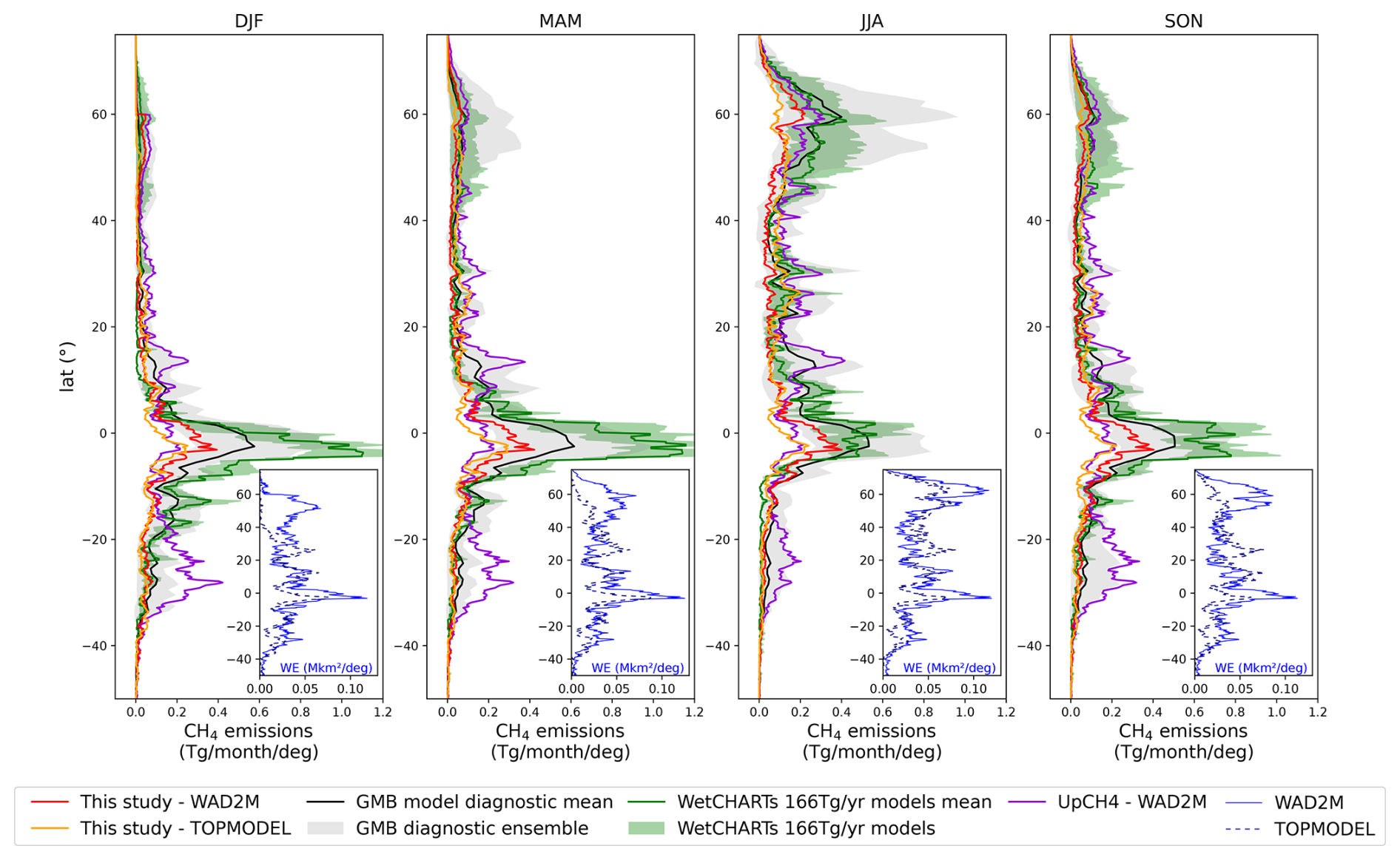
Figure 7 Latitudinal distribution depending on the season of wetland methane emissions from SatWetCH4 run with WAD2M (red) or TOPMODEL (orange), from LSMs (shaded grey) with the LSM average (black), from WetCHARTs models calibrated with a 166 Tg CH₄ yr⁻¹ budget (shaded green) with the ensemble average (green), and from UpCH4 (violet). WAD2M and TOPMODEL wetland extent seasonal means are also presented in bottom-right box inserts (blue solid and dashed lines, respectively). LSM estimates are those contributing to the GMB (Saunois et al., 2020), all run with the same wetland extent product (WAD2M). All representations are 2003–2020 seasonal means.

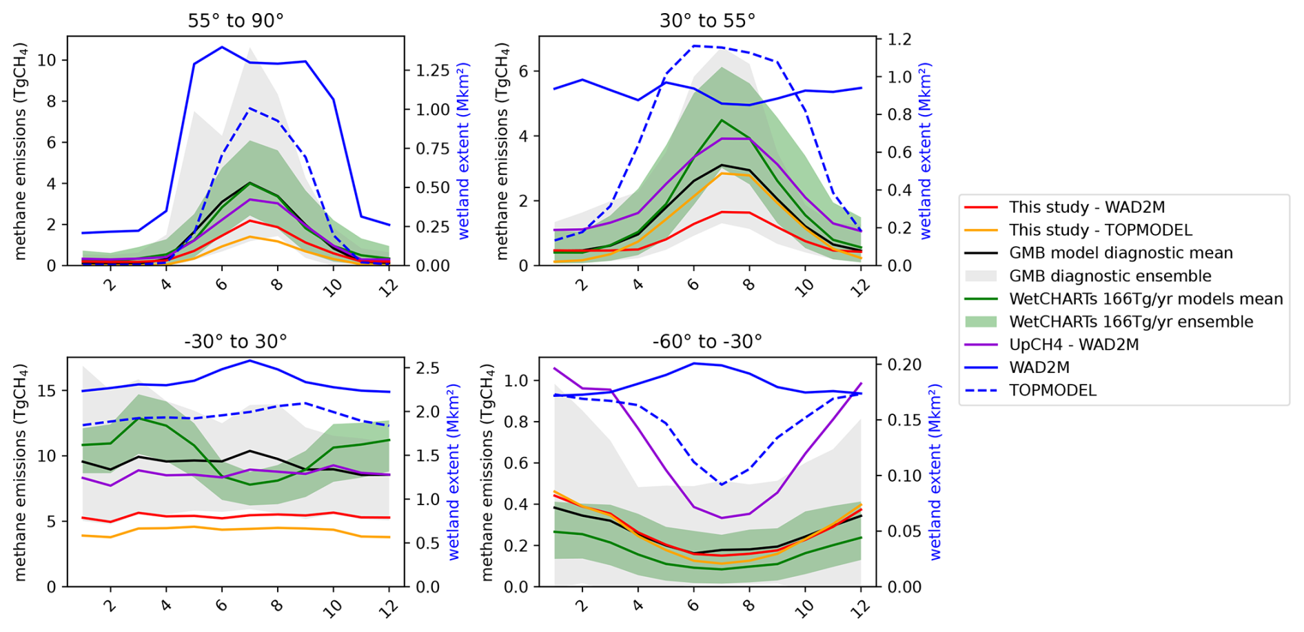
Figure 8 CH₄ emission mean per month per latitudinal band for 2003–2020 from SatWetCH4 run with WAD2M (red) or TOPMODEL (orange), from LSMs (shaded grey) with the LSM average (black), from WetCHARTs models calibrated with a 166 Tg CH₄ yr⁻¹ budget (shaded green) with the ensemble average (green), and from UpCH4 (violet). WAD2M and TOPMODEL monthly wetland extent 2003–2020 means are presented in blue. LSM estimates are those contributing to the GMB (Saunois et al., 2020), all run with the same wetland extent product (WAD2M).

The scarcity of site-level data in tropical regions, coupled with the absence of tropical peatlands and floodplain sites, has undoubtedly contributed to the uncertainty associated with the calibration of parameters. Furthermore, the use of site-level calibration for tropical wetland emission may result in an underestimation at the regional or global scale. This is due to the fact that dynamic wetland mapping products account for saturated or inundated areas, whereas site-level measurements conducted during the dry season are likely to underrepresent the emission intensity of saturated areas. Consequently, the parameters calibrated from dry-season measurements may underestimate emission intensity when multiplied by the area of saturated wetlands. This is a less significant issue in temperate and Arctic regions, where the wet seasons occur in summer and there is minimal emission in winter. As the number of tropical sites increases, future studies could consider refining the calibration for the tropics, for example, by only using wet-season measurements for calibration.

Note that this difference in total emissions could be easily resolved by calibrating the k parameter to the total emissions of the mean GMB LSMs if we need to constrain total emissions as it has been done previously by Bloom et al. (2017) and Gedney et al. (2019).

SatWetCH4 simulation with TOPMODEL estimates lower emissions in the tropical and boreal bands compared to the simulation with WAD2M (Fig. 7). This is consistent with the smallest wetland extent of TOPMODEL over these regions as non-inundated peatlands are not considered in TOPMODEL. Also note the higher fluxes obtained in the simulation with TOPMODEL than with WAD2M around 25–30° N due to the larger wetland extent of TOPMODEL over Asia. The latitudinal distribution of SatWetCH4 (Fig. 7) is consistent with the distribution of the LSMs ensemble, except for the Sahel band mentioned earlier. SatWetCH4 reproduces similar seasonal changes as the GMB LSMs (Fig. 7), while the latitudinal distribution of the WetCHARTs ensemble presents larger emissions in the 10° S–5° N band in the DJF, MAM, and SON seasons (mainly due to high emissions in the Congo region, visible in Fig. 6). UpCH4 presents a different latitudinal distribution, with higher fluxes in the 15° N and 15–35° S bands. These are, respectively, due to the Sahel and Australia artifacts mentioned above. UpCH4 has lower fluxes in the tropical 10° S–5° N band (due to the Amazon and the Congo basins).

This different seasonal cycle in the tropical band (30° S–30° N) for the WetCHARTs ensemble is also visible in Fig. 8, while there is an absence of a pronounced seasonal pattern both in terms of emissions and in terms of wetland extent for our model and the GMB models. This difference in the tropical seasonal cycle could be due to the wetland extent used in WetCHARTs. For the boreal region (55–90° N), we find that the seasonal variation in the simulated emissions from our model is close to that of most GMB LSMs as it is in the northern temperate band (30–55° N). However, the wetland extents of WAD2M and TOPMODEL show very different seasonality, particularly in the northern temperate band (30–55° N), where WAD2M has a more stable wetland extent than TOPMODEL. Indeed, the methane emission seasonality in the boreal and temperate regions is mainly driven by temperature, which explains these similar seasonal cycles in emissions, although the seasonal cycles in the wetland extent are different. For the southern temperate band (60–30° S), WAD2M and TOPMODEL exhibit contrasting seasonality in wetland extent, but the simulated seasonal variations in emissions are close because, as expected, the temperature drives the variability in methane fluxes in this temperate region.

3.3.5 Inter-annual variability in methane emissions at the basin scale

Figure 9 depicts the SatWetCH4 model, GMB LSMs, and UpCH4 emissions simulated with WAD2M and their anomalies for three basins: the Amazon, the Ob, and the Congo. Also shown are wetland areas and their anomalies over these basins.

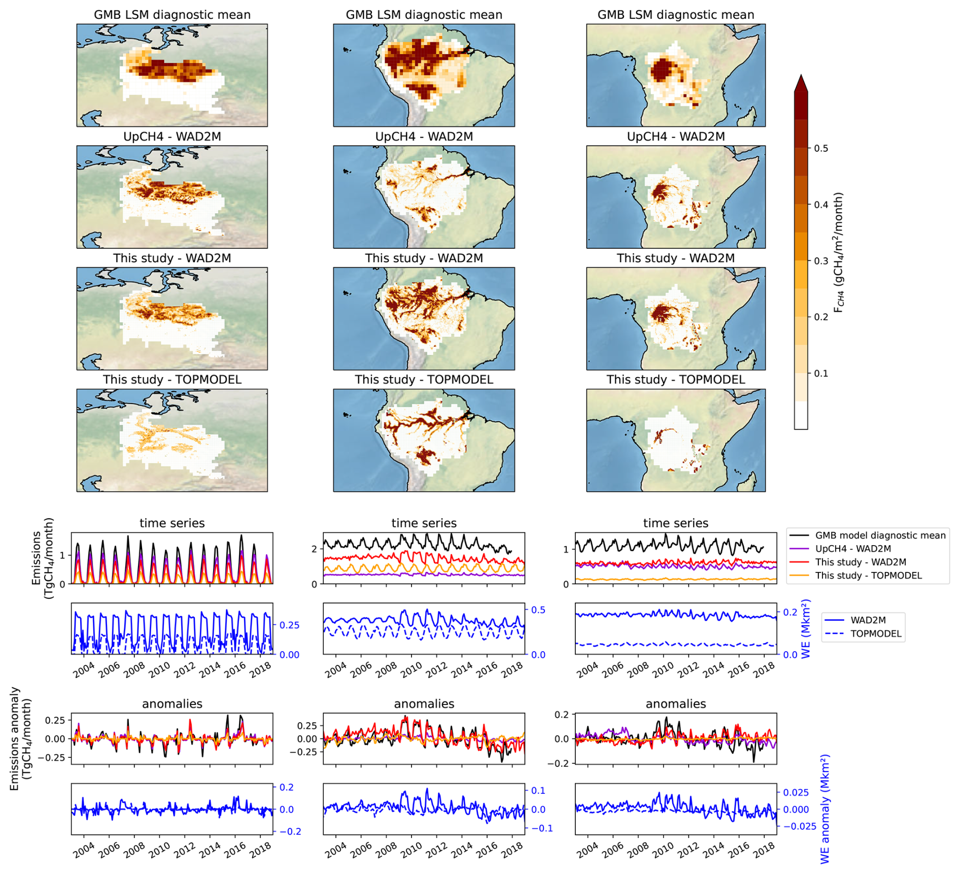
Figure 9 Methane emissions for different basins: the Ob, the Amazon, and the Congo. The maps show the spatial pattern of methane emissions from the GMB LSM means, UpCH4 run with WAD2M, and SatWetCH4 simulations with WAD2M or TOPMODEL. The lower panels represent the sum of methane emission time series and deseasonalized anomalies over the basins of the SatWetCH4 simulations with WAD2M (red) or TOPMODEL (orange), LSM diagnostic mean (black), and UpCH4 simulation with WAD2M (violet). All LSMs were run with the same WAD2M wetland extent. WetCHARTs ensemble is excluded here because its methane emission estimates are rescaled to the average values of the GMB LSM estimates.

In the Amazon and Congo basins, notable amplitude irregularities were observed when using WAD2M in SatWetCH4 or UpCH4. Two regime changes are observed in the WAD2M extent around 2009 and 2014, probably due to inter-calibration problems caused by satellite changes in the original SWAMPS surface water product. Surprisingly, the average of the LSMs is less affected even though the LSMs are forced with the same water surface. However, on closer examination of individual LSMs (see Fig. S5 in the Supplement), we see that some LSMs are as affected as SatWetCH4 by these inconsistent water surface changes, while others are less affected. We deduce that these models, which are not affected by the WAD2M temporal changes, must have parameters that interfere with the consideration of the wetland surface. TOPMODEL suggests more consistent time series in terms of wetland extent (softer variations), which also allows for more realistic variations in terms of emissions.

4 Model limitations and outlook

The simplified approach used here as a one-step model allows for some quick and easy simulations, representing major first-order phenomena affecting methane emissions from wetlands. While presenting a smaller annual budget, due to a possible underestimation of the magnitude of emissions, we found that this formulation presents realistic spatial and temporal variations when compared to other more complex and computationally intensive models. By scaling the k factor to a target estimate, the discrepancy in global emissions could be easily resolved.

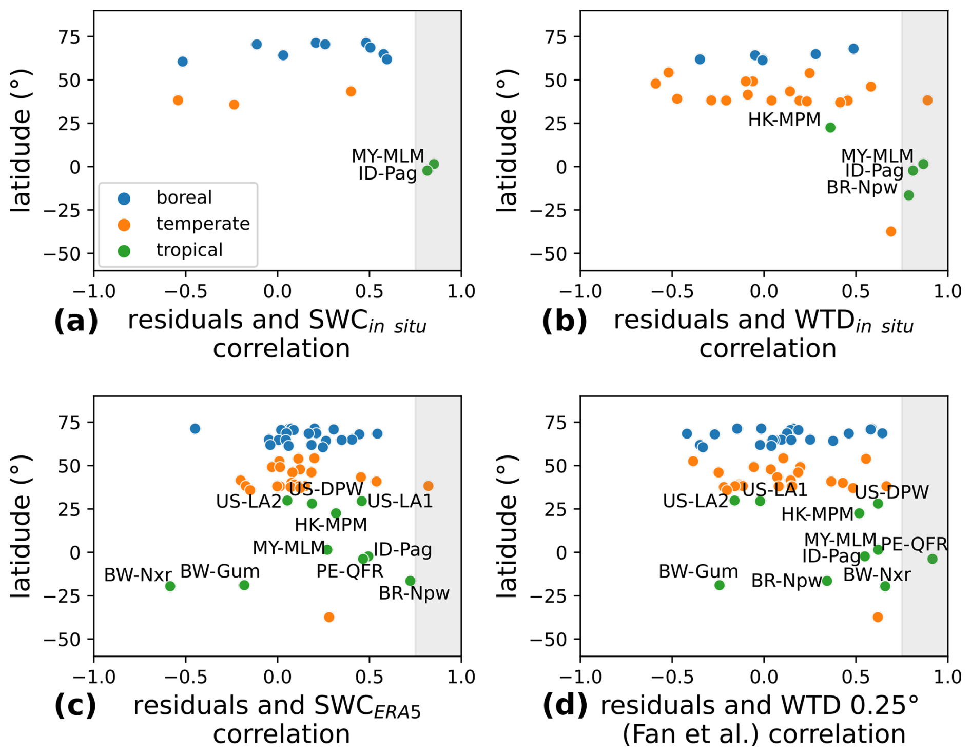
Figure 10 Correlation of residuals (observation–prediction) with (a) in situ WTD, (b) in situ SWC, (c) 0.25° ERA5-Land SWC, and (d) 0.25° WTD (Fan et al., 2013). These residuals are calculated for a single-site calibration of SatWetCH4 in order to remove the seasonal cycle that the model can capture through its variables (soil temperature and substrate availability). The grey background represents an r>0.75.

Some refinements could be considered to improve the accuracy of the model. We found that the simulated temporal variability is captured less well at tropical sites than at temperate and boreal sites as temperature does not drive seasonality in these regions. In fact, some studies (Kuhn et al., 2021; Knox et al., 2021) suggest that methane emissions in tropical regions are influenced by WTD. To investigate the flux dependence on a local water parameter, we calculated residuals from the single-site calibration presented in Sect. 3.2. A residual is the difference between observed and predicted methane fluxes and thus represents the error of the model at a given site at a given time. Figure 10 illustrates the correlation of different hydrological variables with the residuals. In the tropics, the missing variability appears to be strongly linked to soil water variations: two out of two (MY-MLM and ID-Pag) tropical sites monitoring SWC show a strong temporal correlation (r>0.75) of residuals with locally measured SWC, and three out of four sites monitoring WTD (HK-MPM, MY-MLM, ID-Pag, and BR-Npw) show a strong temporal correlation (r>0.75) of residuals with locally measured WTD.

To test whether this site-level correlation could be used in the SatWetCH4 model, we repeat this experiment using global datasets at 0.25° of SWC and WTD. For each site, we selected the nearest 0.25° pixel of the ERA5-Land monthly averaged SWC dataset (available at https://cds.climate.copernicus.eu/, last access: 4 June 2024) and the nearest pixel of the WTD from Fan et al. (2013) aggregated at 0.25° (as only one typical year is provided, this year is replicated for all years of the in situ flux measurement period). Figure 10c and d show the resulting correlation of these two variables at 0.25° with the residuals. None of the 11 tropical sites show an r>0.75 between residuals and ERA5-Land SWC, and only one site (PE-QR) shows an r>0.75 between residuals and 0.25° WTD. This is due to the fact that these 0.25° datasets poorly represent the temporal variations measured in situ, as shown in Fig. S3 in the Supplement for the ERA5-Land SWC. SWC and WTD in wetlands have very spatially localized specificities and variations. Furthermore, the small number of sites available in the tropics (11) makes it even more difficult to find an empirical relationship with a water variable. We were unable to include this important parameter at SatWetCH4 model resolution of 0.25°. The 100 m satellite-derived SWC obtained by Planet (De Jeu et al., 2014) could be examined and the model run at a finer resolution. In fact, Albuhaisi et al. (2023) found an improvement in their model for the boreal region when using this high-resolution product. Further research could be conducted to see if similar results are obtained in the tropics, where this parameter is the most needed. Unfortunately, this product is not freely available.

It is worth noting that the site-level comparison of modeled fluxes with observations assumes that the sites are all wetlands (f_w=1) without any temporal variation. However, when the SatWetCH4 model is run, this wetland fraction is dynamic, introducing seasonality due to water and partially compensating for the lack of a local water parameter.

Another limitation is that the consistency of the time series of methane emission estimates at the catchment scale is strongly affected by errors in the WAD2M database. This makes it difficult to study inter-annual variability or trends. The TOPMODEL time evolution does not have these major temporal inconsistencies, but it is based on a hydrological model and not on satellite observations. It also does not include non-inundated peatlands. An improved satellite-derived dynamic wetland surface map would be crucial to address these issues while maintaining observational data in our data-driven approach.

The simplified SatWetCH4 model we have developed makes important approximations that imply important shortcuts. In particular, no distinction is made between methane production and emissions. This supposes that SatWetCH4 one-step equation includes production, oxidation, and transport in a single formulation, which are sometimes distinguished in some of the more complex LSMs (Wania et al., 2013; Morel et al., 2019; Salmon et al., 2022). Among the three pathways of methane transport in wetlands, including diffusion, ebullition, and plant-mediated transport, plant-mediated transport is the dominant one (Ge et al., 2024). Ge et al. (2024) have recently published a comprehensive review of the role of plants in methane fluxes, showing their influence on not only methane transport but also methane production and oxidation. Feron et al. (2024) also show that trends in methane flux changes at the site level depend on the ecosystem and vegetation type. Accounting for the different vegetation classes therefore appears to be a possible improvement to our simplified approach.

A simple way to account for this in the SatWetCH4 model at the first order would be to fit the scaling factor k and/or $Q_{\mathrm{10}}^{\mathrm{0}}$ as a function of the vegetation class or wetland type. Indeed, Q₁₀ was found to depend on ecosystems (Chang et al., 2021). We performed such calibration tests, taking into account the wetland classification. However, the cost function either did not converge due to the small number of sites per category or displayed a result that was highly dependent on few sites, thus overfitting results. In fact, eddy covariance flux towers measuring methane emissions are not evenly distributed around the globe, and their distribution is highly skewed, as discussed in Sect. 2.2. Some wetland categories are poorly represented, for example, there are only two mangrove sites. This scarcity of data makes this type of calibration highly uncertain. However, we can expect an improvement in the coming years as in situ methane measurement is a rapidly growing field, as shown by the increasing number of flux towers along the years in Table S1 in the Supplement. Future data, especially in the tropics, will be essential to better constrain the models and to take more processes into account. Some refinement of the Q₁₀ function (here $Q_{\mathrm{10}}\left(T\right)=Q_{\mathrm{10}}^{\mathrm{0}}{}^{T^{\mathrm{0}}/T}$ according to Gedney, 2004) could be envisioned, such as the incorporation of a hysteresis (Chang et al., 2021).

Despite the impossibility of analyzing temporal variation due to WAD2M issues, Fig. 9 informs us that the temporal variations of SatWetCH4 are more similar to GMB LSMs than UpCH4. This is consistent with the fact that SatWetCH4 is a – highly simplified – process-based equation, whereas UpCH4 relies on empirical flux upscaling using random forest. SatWetCH4 and UpCH4 approaches both provide new independent estimates of wetland emissions, while offering distinct perspectives. A deeper comparison of the fluxes modeled by SatWetCH4 and UpCH4 at the site level could serve understanding differences between the simplification of complex processes represented by a fixed process equation (SatWetCH4) versus a pure machine learning data-driven approach (UpCH4). In addition, running both SatWetCH4 and UpCH4 with another wetland extent database would also serve to assess uncertainties and errors associated with the WAD2M product and a better comparison of global methane emission trends estimated by SatWetCH4 and UpCH4. Both methods are currently limited by the scarcity of eddy covariance flux data (McNicol et al., 2023), especially over important wetland methane-emitting regions of the world, e.g., in the tropics (the Congo, the Sudd, and the Amazon) and Russia (Siberian lowlands).

5 Conclusions

SatWetCH4 model was developed to simulate global wetland methane emissions at 0.25° × 0.25° with a monthly time resolution. This data-driven approach was calibrated with 58 sites of eddy covariance flux data, allowing for an approach independent of other estimates. Most of SatWetCH4 model input variables are derived from satellite observational products. In particular, a new estimate of the substrate availability was derived using MODIS-derived NPP. This product, called C_substrate, appears to be a more realistic approach than in previous studies that considered all SOC to be available carbon.

At the site level, the SatWetCH4 calibration reproduces the boreal fluxes and most of the temperate fluxes well but reproduces the emissions seasonality of the tropical sites poorly. This could possibly be improved in future studies by adding high-resolution information on local water availability (SWC). Another important improvement would be a calibration per the wetland type, which would allow for the influence of vegetation to be taken into account as major transport pathways. For this, more eddy covariance flux measurements in the tropics are essential to gain a deeper insight into the processes governing temporal variations in this latitudinal band and to develop and calibrate this one-step model.

SatWetCH4's simple formulation allows for fast global simulations (within a few seconds) over decades using satellite observations as input data. Although the total methane emission estimates from SatWetCH4 are lower than those reported in the literature (Saunois et al., 2020; McNicol et al., 2023), SatWetCH4 shows that it is able to reproduce large spatio-temporal variations at 0.25°, which makes it a useful tool to study methane emission inter-annual trends. Thus, the SatWetCH4 model benefit from independent remote-sensing data and from a process-based model approach since it is calibrated using in situ site observations.

Finally, we found some inconsistencies in the widely used WAD2M surface wetland extent. A new wetland map is currently being produced (Bernard et al., 2024b) based on GIEMS-2 (Prigent et al., 2020) observations which provide a seamless estimate of inundated areas with realistic inter-annual variability (Bernard et al., 2024a). Utilizing the SatWetCH4 model with this new dataset would allow for the study of annual variability and trends in emissions.

Another perspective is the coupling of SatWetCH4 with atmospheric inversions. Indeed, one way to overcome the challenges associated with calibration using surface flux data is to incorporate this simple model into an atmospheric inversion model. This would allow for the optimization of both parameters k and $Q_{{\mathrm{10}}_{\mathrm{0}}}$ in the inversion equation using atmospheric concentrations (more numerous than methane fluxes data, especially with satellite data) rather than just the optimization of the methane flux value, as is usually done in inversion models.