Automatic optical depth parametrization in radiative transfer model RTTOV v13 via LASSO-induced sparsity

The assimilation of satellite spectral sounder data requires fast and accurate radiative transfer models. This study proposes a novel methodology to automatically parameterize atmospheric optical depths within the Radiative Transfer for TOVS (RTTOV) version 13 scheme using statistical thresholds across pressure levels and Least Absolute Shrinkage and Selection Operator (LASSO) regression to induce sparsity. Numerical experiments with Visible Infrared Imaging Radiometer Suite (VIIRS) infrared channels demonstrate that this approach significantly reduces computational costs while maintaining accuracy. The sparsity also facilitates the automatic selection of absorbing gases and predictors by channel and pressure level, making it particularly effective for multispectral instruments with numerous atmospheric variables. These findings highlight the potential of sparse regression methods to enhance the efficiency of radiative transfer models for satellite data assimilation.

1 Introduction

In satellite data assimilation and remote sensing retrievals, as well as their applications in numerical weather prediction (NWP), the radiative transfer equation (RT) is the main model used to retrieve global atmospheric variables, such as temperature and trace gases concentrations, including water vapor, ozone, carbon dioxide, and other atmospheric constituents. This is achieved by utilizing top of the atmosphere (TOA) radiance measurements from satellite sounders operating across different channels of the electromagnetic spectrum. The numerical implementation of the RT equation as a forward model can primarily be carried out using two approaches: Line-by-Line (LBL) Radiative Transfer models and Fast Radiative Transfer models (Fast-RT).

Line-by-line models simulate satellite radiance by rigorously integrating atmospheric physics and chemical phenomena. These models are highly accurate in replicating the precision of modern instruments, such as hyperspectral sounders like AIRS, CrIS and IASI. However, they are characterized by significant computational demands in terms of CPU time and memory, making them impractical for use in operational data assimilation. Some of the most well-known models in this category include: LBLRTM, developed at Atmospheric and Environmental Research, Inc. (AER) (Clough et al., 1992; Clough and Iacono, 1995; Clough et al., 2005); AMSUTRAN, developed at the Met Office (UK) (Turner et al., 2019); and GENLN2, developed at the National Center for Atmospheric Research (NCAR) (Edwards, 1992). A comparison between LBLRTM and GENLN2 is presented in Matricardi (2007). Another software worth mentioning is kCARTA (DeSouza-Machado et al., 2020), a pseudo Line-by-Line model that uses precomputed and compressed physically intensive processes in RT model to compute radiances more quickly while maintaining accuracy.

On the other hand, the most common Fast-RT models estimate the expected radiance in a channel (what a sensor actually measures) and are typically based on statistical approaches. In these models, the complex and computationally costly physical processes of RT modeling, the calculation of atmospheric transmittances, are parameterized using statistical models and trained with output from Line-by-Line software on real atmospheric profile databases. The parameters are adjusted using standard linear regression models or other machine learning techniques. While these methods sacrifice a small degree of accuracy, they significantly reduce computational costs, making them practical for use in operational data assimilation. Some of the most well-known models in this category include: OPTRAN, developed by the NESDIS-NCEP community (McMillin et al., 1995; Kleespies et al., 2004; McMillin et al., 2006); the Joint Center for Satellite Data Assimilation (JCSDA) Community Radiative Transfer Model (CRTM) (Han et al., 2006; Chen et al., 2008); and the RTTOV model, see (Saunders et al., 2018) and the references therein. Other studies using statistical approaches include Matricardi (2010), which incorporates principal component analysis in RTTOV, as well as (Liu et al., 2009; Krishnan et al., 2012; Cao et al., 2021; Stegmann et al., 2022; Mauceri et al., 2022; Su et al., 2023), which apply machine learning techniques for parametrization, feature reduction, and sampling strategies.

Even though RTTOV is more efficient than line-by-line models, it remains prohibitively expensive for operational use cases¹. Indeed, in current Fast RT models based on linear regression, such as OPTRAN and RTTOV, training is performed separately for each gas type and pressure level, resulting in an over-parametrization of the RT model. To reduce the number of parameters and make the evaluation of the trained RT model less computationally expensive, it is essential to carefully select the most significant gases for each spectral channel of each instrument type, reduce the number of pressure levels, and implement other ad hoc strategies. These decisions must account for the large number of possible combinations and trade-offs, and are typically made by expert teams.

One promising approach to reducing the number of parameters without relying on expert committees is the use of optimization methods that induce sparsity in the parameters. In particular, the use of LASSO regression, a regularization method that penalizes the regression coefficients with the ℓ₁-norm, has proven effective for variable selection and model complexity reduction in various large-scale applications (see, e.g., Heilemann et al., 2024; Pak et al., 2025). In the context of radiative transfer, LASSO regression was applied by Cardall et al. (2023) to estimate water quality parameters such as clarity, temperature, and chlorophyll a, based on correlations with in-situ measurements and near-coincident Landsat spectral data, with a focus on model explainability. In Li et al. (2020), the authors proposed an algorithm for detecting hazardous clouds using passive infrared remote sensing technology with variable selection. Other studies that combine or compare LASSO with machine learning methods for remote sensing include: the removal of redundant features in PolSAR and optical images (Hong and Kong, 2021); estimation of aboveground forest biomass with variable selection (Wang et al., 2022a); identification of important environmental variables for retrieving soil moisture content (Wang et al., 2022b); evaluation of the accuracy and generalization capacity of grassland models (Smith et al., 2023); and a comparison of different machine learning methods for predicting soybean yield (Joshi et al., 2023).

Building on this approach, in this paper we target the automatic selection of gases and optical depth predictors in Fast RT models by inducing sparsity in the weight predictors using LASSO regression. We propose a parametrization of transmittances based on statistical thresholds to automatically select the appropriate gases by channel and pressure level, and to induce sparsity in the parameters by replacing the classical regression problem with a LASSO problem within the RTTOV framework. The proposed methodology is tested with VIIRS infrared channels, and the results are compared with the standard RTTOV model. To the best of the authors' knowledge, this is the first time that LASSO regression has been applied to the RTTOV model to automate the selection of gases and parameters.

One of the key aspects in LASSO models is the choice of the regularization weight in front of the ℓ₁-norm. This weight controls the trade-off between fitting the training data well and keeping the model simple by reducing the number of non-zero coefficients. In our context, selecting an appropriate regularization weight is crucial for effectively identifying the most relevant gases and optical depth predictors while avoiding overfitting. To establish a rigorous criterion for choosing this parameter – rather than relying on a tedious trial-and-error process – we propose a bilevel optimization approach (see, e.g., De los Reyes and Villacís, 2022; De los Reyes, 2023). The idea is to formulate an upper-level optimization problem that encodes a model quality criterion, while the LASSO problem serves as the lower-level constraint. In this article, we successfully test two types of loss functions: the first, based on an ℓ₀ seminorm that prescribes the number of non-zero predictors; and the second, inspired by a Bayesian Information Criterion-type objective.

This manuscript is organized as follows: Sect. 2 outlines the theoretical framework for the RT equation in Line-By-Line models and details the general scheme of Fast-RT methods, focusing on RTTOV. Section 3 introduces the proposed transmittance parametrization using statistical inference and LASSO regression model, as well as the bilevel optimization approach for selecting the regularization weight. Section 4 presents the experimental settings and numerical results comparing RTTOV with the proposed method. Finally, Sect. 5 offers conclusions of the performance of the proposed approach.

2 Radiative Transfer Equation

The monochromatic radiative transfer equation for the upwelling radiance in a clear sky, without solar radiation contribution, for a non-scattering atmosphere and in local thermodynamic equilibrium, is given by:

$$\begin{array}{}\text{(1)}& \begin{array}{rl}I(\mathit{\nu },\mathit{\theta })& ={\mathit{\tau }}_{\mathrm{s}}(\mathit{\nu },\mathit{\theta }){\mathit{ϵ}}_{\mathrm{s}}(\mathit{\nu },\mathit{\theta })B(\mathit{\nu },T_{\mathrm{s}})+\underset{{\mathit{\tau }}_{\mathrm{s}}}{\overset{\mathrm{1}}{\int }}B(\mathit{\nu },T(p\left)\right)d\mathit{\tau }\\ & +(\mathrm{1}-{\mathit{ϵ}}_{\mathrm{s}}(\mathit{\nu },\mathit{\theta }\left)\right){\mathit{\tau }}_{\mathrm{s}}^{\mathrm{2}}(\mathit{\nu },\mathit{\theta })\underset{{\mathit{\tau }}_{\mathrm{s}}}{\overset{\mathrm{1}}{\int }}{\displaystyle \frac{B(\mathit{\nu },T(p\left)\right)}{{\mathit{\tau }}^{\mathrm{2}}}}d\mathit{\tau },\end{array}\end{array}$$

where I(ν,θ) is the monochromatic TOA radiance at wavenumber ν and satellite zenith angle θ; B(ν,T) is the Planck function at temperature T; $\mathit{\tau }(\mathit{\nu },\mathit{\theta },p,T,q)$ denotes the layer-to-space transmittance dependent on pressure p, temperature T, and gas concentration q. Here, T_s, ϵ_s, and τ_s represent surface skin temperature, emissivity, and transmittance respectively, (Weinreb et al., 1981).

The terms correspond to surface emission, upward atmospheric emission, and downward atmospheric emission reflected at the surface (assuming specular reflection). Surface emissivity can be close to 1 for ν between 714–1250 cm⁻¹ and for surfaces such as bodies of water, ice and healthy plant leaves, carbon powder, allowing the last term to be discarded.

The model described above, computed for each wavenumber ν is called the Line-by-Line model, and the resulting radiance is monochromatic.

Satellite-measured radiance is polychromatic, simulated by convolving Eq. (1) with the instrument's Normalized Spectral Response Function (NSRF):

$$\begin{array}{}\text{(2)}& \stackrel{\mathrm{‾}}{I}({\mathit{\nu }}^{*},\mathit{\theta })=\underset{{\mathit{\nu }}_a}{\overset{{\mathit{\nu }}_b}{\int }}\mathit{\varphi }(\mathit{\nu },{\mathit{\nu }}^{*})I(\mathit{\nu },\mathit{\theta })d\mathit{\nu },\end{array}$$

where $\mathit{\varphi }(\mathit{\nu },{\mathit{\nu }}^{*})$ is the NSRF, representing the sensitivity to radiance within the spectral channel [ν_a,ν_b], with ν^* representing the centroid of the response. Using the expression (2) in Eq. (1), the polychromatic radiance for the spectral channel identified with ν^*, assuming ϵ_s=1, can be written as (see Weinreb et al., 1981):

$$\begin{array}{}\text{(3)}& \stackrel{\mathrm{‾}}{I}({\mathit{\nu }}^{*},\mathit{\theta })={\stackrel{\mathrm{‾}}{\mathit{\tau }}}_{\mathrm{s}}({\mathit{\nu }}^{*},\mathit{\theta })B(\mathit{\nu },T_{\mathrm{es}})+\underset{{\mathit{\tau }}_{\mathrm{s}}}{\overset{\mathrm{1}}{\int }}B({\mathit{\nu }}^{*},T_{\mathrm{e}}(p\left)\right)d\stackrel{\mathrm{‾}}{\mathit{\tau }},\end{array}$$

where T_es and T_e are empirical effective temperatures obtained via regression. The polychromatic transmittance is given by:

$$\begin{array}{}\text{(4)}& \stackrel{\mathrm{‾}}{\mathit{\tau }}({\mathit{\nu }}^{*},\mathit{\theta },p,T,q)=\underset{{\mathit{\nu }}_a}{\overset{{\mathit{\nu }}_b}{\int }}\mathit{\varphi }(\mathit{\nu },{\mathit{\nu }}^{*})\mathit{\tau }(\mathit{\nu },\mathit{\theta },p,T,q)d\mathit{\nu }.\end{array}$$

Transmittance follows Beer-Lambert law $\mathit{\tau }=e^{-d}$, with optical depth $d(\mathit{\nu },\mathit{\theta },p,T,q)$ accounting for absorption by gases (e.g., H₂O, O₃, CO₂, CH₄) and continuum effects. The monochromatic optical depth for a set of gases ${\mathit{g}}_{\mathrm{1}},\mathrm{\dots },{\mathit{g}}_{\mathrm{s}}$ is:

$$\begin{array}{}\text{(5)}& \begin{array}{rl}d(\mathit{\nu },\mathit{\theta },p,T,q)& =-{\displaystyle \frac{\sec \left(\mathit{\theta }\right)}{g}}\sum _{l=\mathrm{1}}^s\\ & \underset{\mathrm{0}}{\overset{p}{\int }}{K}^{{\mathit{g}}_l}(\mathit{\nu },p^{\prime },T(p^{\prime }\left)\right)q^{g_l}\left(p^{\prime }\right)d{p}^{\prime },\end{array}\end{array}$$

where g is gravitational acceleration, $K^{{\mathit{g}}_l}$ is the absorption function modeled via Voigt profiles (see Lavrentieva et al., 2011).

2.1 Fast Radiative Transfer Model

Fast RT models discretize the atmosphere into L layers:

$$p_{\mathrm{0}}<p_{\mathrm{1}}<\mathrm{\cdots }<p_L,$$

where p₀ is the top-of-atmosphere and p_L the surface pressure. Polychromatic radiance Eq. (3) is computed numerically, requiring parameterization of polychromatic transmittance to reduce computational cost. In Fast-RT models, the polychromatic optical depth is parameterized and fitted via linear regression to approximate Eq. (5), following ideas from McMillin and Fleming (McMillin and Fleming, 1976; Fleming and McMillin, 1977; McMillin et al., 1979).

The polychromatic optical depth from layer i to the top of the atmosphere, for a single channel and gas g_l, is:

$$\begin{array}{}\text{(6)}& d_i^{{\mathit{g}}_l}=d_{i-\mathrm{1}}^{{\mathit{g}}_l}+\sum _{j=\mathrm{1}}^{m_l}{w}_{ij}^{{\mathit{g}}_l}{X}_{ij}^{{\mathit{g}}_l},d_{\mathrm{0}}^{{\mathit{g}}_l}=\mathrm{0},i=\mathrm{1},\mathrm{\dots },L,\end{array}$$

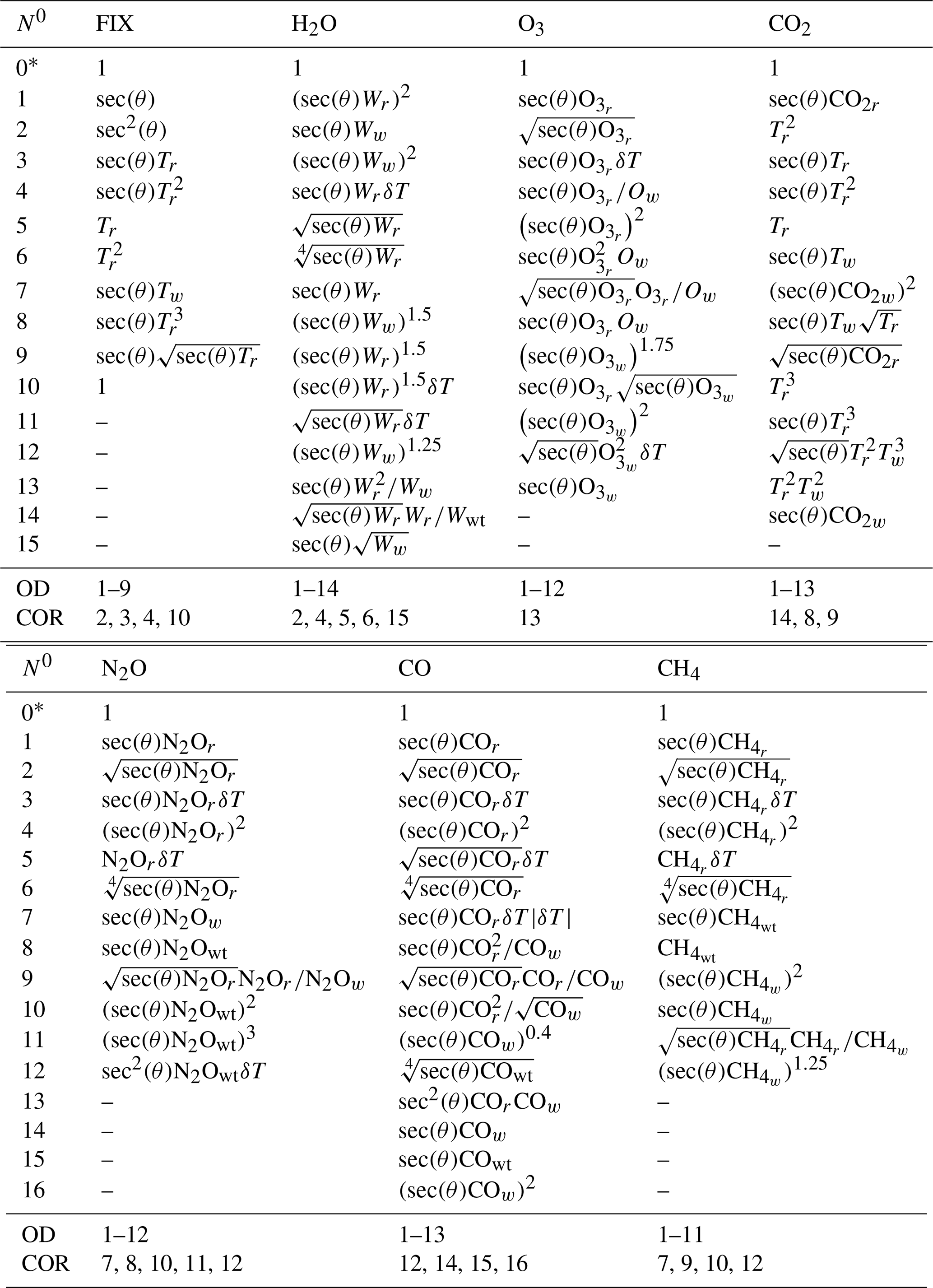
where $X_{ij}^{{\mathit{g}}_l}$ are predictors depending on view angle, temperature, and gas concentration. The parameters $w_{ij}^{{\mathit{g}}_l}$ define the model. Appendix B provides details on the RTTOV v13 predictors, and further information can be found in Saunders et al. (2017).

This parametrization includes a fixed gas mixture – whose spatio-temporal variations minimally affect radiance – and variable gases, primarily H₂O, optionally including O₃, CO₂, N₂O, CO, CH₄, and SO₂, varying by channel. Water vapor absorption may be split into line and continuum components.

The polychromatic transmittance of layer i for gas g_l is approximated by:

$$\begin{array}{}\text{(7)}& {\mathit{\tau }}_{(i,\mathrm{0})}^{{\mathit{g}}_l}=\exp (-d_i^{{\mathit{g}}_l}),\end{array}$$

and total transmittance approximated as:

$$\begin{array}{}\text{(8)}& {\mathit{\tau }}_{(i,\mathrm{0})}^{\mathrm{TOT}}=\prod _{l=\mathrm{1}}^s{\mathit{\tau }}_{(i,\mathrm{0})}^{{\mathit{g}}_l}.\end{array}$$

Parameters are fitted using a database of M vertical atmospheric profiles:

$$(p_i,T_{ij},q_{ij}^{{\mathit{g}}_{\mathrm{1}}},\mathrm{\dots },q_{ij}^{{\mathit{g}}_{\mathrm{s}}}),i=\mathrm{0},\mathrm{\dots },L,j=\mathrm{1},\mathrm{\dots },M,$$

with polychromatic transmittances computed with Line-by-Line software for N view angles θ_k:

$$\begin{array}{}\text{(9)}& \begin{array}{rl}({\mathit{\tau }}_{ijk}^{{\mathit{g}}_{\mathrm{1}}},& \mathrm{\dots },{\mathit{\tau }}_{ijk}^{{\mathit{g}}_{\mathrm{s}}}),i=\mathrm{1},\mathrm{\dots },L,\\ & j=\mathrm{1},\mathrm{\dots },M,k=\mathrm{1},\mathrm{\dots },N.\end{array}\end{array}$$

Since total polychromatic transmittance is not simply the product of individual gases transmittances (unlike the monochromatic case), data (9) are corrected following (Xiong and McMillin, 2005; McMillin et al., 2006), as in RTTOV v13 (Hocking et al., 2021), by introducing a corrective term ${\mathit{\tau }}_{(i,\mathrm{0})}^{\mathrm{COR}}$:

$$\begin{array}{}\text{(10)}& {\mathit{\tau }}_{(i,\mathrm{0})}^{\mathrm{TOT}}={\mathit{\tau }}_{(i,\mathrm{0})}^{\mathrm{COR}}\prod _{l=\mathrm{1}}^s{\mathit{\tau }}_{(i,\mathrm{0})}^{{\mathit{g}}_l},\end{array}$$

which is parameterized similarly to Eqs. (6) and (7). The corrective transmittance for training is:

$${\mathit{\tau }}_{ijk}^{\mathrm{COR}}={\displaystyle \frac{{\mathit{\tau }}_{ijk}^{\mathrm{TOT}}}{{\widehat{\mathit{\tau }}}_{ijk}^{\mathrm{TOT}}}},$$

where ${\mathit{\tau }}_{ijk}^{\mathrm{TOT}}$ is the Line-by-Line polychromatic transmittance including all absorbers, and ${\widehat{\mathit{\tau }}}_{ijk}^{\mathrm{TOT}}$ is the modeled transmittance from Eq. (8).

The linear regression fitting problem for gas g_l and layer i is:

$$\begin{array}{}\text{(11)}& \left({\mathrm{LS}}_{{\mathit{g}}_l}\right)\underset{{\mathit{w}}_i^{{\mathit{g}}_l}\in {\mathbb{R}}^{m_l}}{min}{\displaystyle \frac{\mathrm{1}}{\mathrm{2}MN}}{∥A_i^{{\mathit{g}}_l}{\mathit{w}}_i^{{\mathit{g}}_l}-{\mathit{y}}_i^{{\mathit{g}}_l}∥}_{\mathrm{2}}^{\mathrm{2}},\end{array}$$

where $A_i^{{\mathit{g}}_l}\in {\mathbb{R}}^{MN\times m_l}$ contains predictors $X_{ij}^{{\mathit{g}}_l}$ for angles, temperatures, and concentrations across profiles, and ${\mathit{y}}_i^{{\mathit{g}}_l}\in {\mathbb{R}}^{MN}$ the corresponding optical depths.

In RTTOV v13, parameter counts per channel reach nearly 11 000, considering variable and fixed gases, layers, and corrections. Reduction is achieved by expert-based gas selection, layer thinning, and thresholding (see Saunders et al., 2017).

3 A Sparse Parametrization of Optical Depths

In this section, we present a methodology to significantly reduce the number of parameters used in optical depth parametrization within the RTTOV v13 framework. The methodology involves automatically selecting absorbing gases per channel and pressure level, as well as identifying the most important predictors for each atmospheric layer. This approach induces sparsity in the regression parameters by combining two tools: statistical inference to determine whether a given gas at a particular layer requires no parametrization, a parametrization with a single predictor, or a more complex parametrization as described in Eq. (6). In the latter case, the classic linear regression problem is replaced with a LASSO regression problem to select predictors and induce sparsity in the parameter vectors.

3.1 Parametrization Based on Statistical Inference

The aim here is to preprocess the data of the polychromatic transmittances in a channel to determine which atmospheric layers require optical depth parametrization and to automatically exclude gases that do not significantly contribute to the radiance absorption in that channel. To achieve this, we will use confidence intervals to estimate the true polychromatic transmittances.

For a gas g_l or correction term in a fixed layer i, we construct a confidence interval for the mean of the polychromatic transmittances of the layer i. This is given by:

$$\left[{\stackrel{\mathrm{‾}}{\mathit{\tau }}}_i^{{\mathit{g}}_l}-E_i^{{\mathit{g}}_l},{\stackrel{\mathrm{‾}}{\mathit{\tau }}}_i^{{\mathit{g}}_l}+E_i^{{\mathit{g}}_l}\right]$$

where

$$E_i^{{\mathit{g}}_l}=Z_{\mathrm{1}-\frac{\mathit{\alpha }}{\mathrm{2}}}{\displaystyle \frac{s_i^{{\mathit{g}}_l}}{\sqrt{NM}}},$$

${\stackrel{\mathrm{‾}}{\mathit{\tau }}}_i^{{\mathit{g}}_l}$ is the mean polychromatic transmittance for layer i, considering N angles and M atmospheric profiles, $s_i^{{\mathit{g}}_l}$ is the corresponding standard deviation, and $Z_{\mathrm{1}-\frac{\mathit{\alpha }}{\mathrm{2}}}$ is the critical value of a distribution for a confidence level of 1−α. Given that the number of data points in each layer is NM, which is usually sufficiently large (in our experiments, for N=6 angles and M=83 profiles, NM=498), the standard normal distribution is used to obtain the critical value. Thus, the absolute error in approximating the true value of the polychromatic transmittance of gas g_l in layer i, with ${\stackrel{\mathrm{‾}}{\mathit{\tau }}}_i^{{\mathit{g}}_l}$ is at most $E_i^{{\mathit{g}}_l}$, with a probability α that the absolute error exceeds this value. In our case, the confidence level is set to $\mathit{\alpha }={\mathrm{10}}^{-\mathrm{6}}$.

Based on the above, the following statistical thresholds for optical depth parametrizations are proposed. Let ϵ₁ and ϵ₂ be positive and sufficiently small values, these will be used as thresholds to determine whether ${\stackrel{\mathrm{‾}}{\mathit{\tau }}}_i^{\mathit{g}l}$ is close to the true value or close to 1. Define the mean optical depth for layer i as ${\stackrel{\mathrm{‾}}{d}}_i^{{\mathit{g}}_l}=-\ln \left({\stackrel{\mathrm{‾}}{\mathit{\tau }}}_i^{{\mathit{g}}_l}\right)$, and consider the following three cases:

• Case I. If $E_i^{{\mathit{g}}_l}>{\mathit{ϵ}}_{\mathrm{1}}$, the polychromatic transmittance due to gas g_l in layer i has high variability with respect to the value of the atmospheric variables in that layer. In this case, the optical depth parametrization follows as in Eq. (6) for layer i.

• Case II. If $E_i^{\mathit{g}l}\le {\mathit{ϵ}}_{\mathrm{1}}$ and ${\stackrel{\mathrm{‾}}{d}}_i^{{\mathit{g}}_l}>{\mathit{ϵ}}_{\mathrm{2}}$, unlike the previous case, the polychromatic transmittance due to gas g_l in layer i has low variability with respect to the value of the atmospheric variables in that layer, and can be estimated by ${\stackrel{\mathrm{‾}}{\mathit{\tau }}}_i^{{\mathit{g}}_l}$, but is not close to 1. Thus, the optical depth can be parameterized with a single predictor as follows:

  $$d_i^{{\mathit{g}}_l}=d_{i-\mathrm{1}}^{{\mathit{g}}_l}+w_{i\mathrm{0}}^{{\mathit{g}}_l}{X}_{i\mathrm{0}}^{{\mathit{g}}_l},$$

  where, X_0i=1 and $w_{i\mathrm{0}}^{{\mathit{g}}_l}={\stackrel{\mathrm{‾}}{d}}_i^{{\mathit{g}}_l}$. If this occurs in all layers, and since the parametrization does not depend on atmospheric variables, the gas g_l can be included with fixed gases.

• Case III. If $E_i^{{\mathit{g}}_l}\le {\mathit{ϵ}}_{\mathrm{1}}$ and ${\stackrel{\mathrm{‾}}{d}}_i^{{\mathit{g}}_l}\le {\mathit{ϵ}}_{\mathrm{2}}$, the polychromatic transmittance in layer i can not only be estimated by ${\stackrel{\mathrm{‾}}{\mathit{\tau }}}_i^{{\mathit{g}}_l}$ but is also close to 1, meaning that gas g_l does not cause significant absorbance in this layer. The relative error of approximating ${\stackrel{\mathrm{‾}}{\mathit{\tau }}}_i^{{\mathit{g}}_l}$ with 1 is given by:

  $${\displaystyle \frac{\mathrm{1}-{\stackrel{\mathrm{‾}}{\mathit{\tau }}}_i}{{\stackrel{\mathrm{‾}}{\mathit{\tau }}}_i}}=e^{{\stackrel{\mathrm{‾}}{d}}_i^{{\mathit{g}}_l}}-\mathrm{1}={\stackrel{\mathrm{‾}}{d}}_i^{{\mathit{g}}_l}{e}^{\mathit{\xi }}\le {\mathit{ϵ}}_{\mathrm{2}}{e}^{{\mathit{ϵ}}_{\mathrm{2}}}\approx {\mathit{ϵ}}_{\mathrm{2}},$$

  for some $\mathit{\xi }\in (\mathrm{0},{\stackrel{\mathrm{‾}}{d}}_i^{{\mathit{g}}_l})$. If this condition is met for all layers, then gas g_l is automatically discarded.

To summarize the above, the parametrization of optical depths based on statistical thresholds is as follows:

$$\begin{array}{ll}{\displaystyle }& {\displaystyle }{d}_{\mathrm{0}}^{{\mathit{g}}_l}=\mathrm{0}\\ \text{(12)}& {\displaystyle }& {\displaystyle }{d}_i^{{\mathit{g}}_l}=d_{i-\mathrm{1}}^{{\mathit{g}}_l}+\left\{\begin{array}{ll}{\sum }_{j=\mathrm{1}}^{m_l}{w}_{ij}^{{\mathit{g}}_l}{X}_{ij}^{{\mathit{g}}_l},& E_i^{{\mathit{g}}_l}>{\mathit{ϵ}}_{\mathrm{1}},\\ {\stackrel{\mathrm{‾}}{d}}_i^{{\mathit{g}}_l},& E_i^{{\mathit{g}}_l}\le {\mathit{ϵ}}_{\mathrm{1}}\text{ and }{\stackrel{\mathrm{‾}}{d}}_i^{{\mathit{g}}_l}>{\mathit{ϵ}}_{\mathrm{2}},\\ \mathrm{0},& \text{otherwise},\end{array}\right.\end{array}$$

for $i=\mathrm{1},\mathrm{2},\mathrm{\dots },L$. The transmittances from layer i to the top of the atmosphere are still calculated using Eq. (7).

The statistical threshold tolerances ϵ₁ and ϵ₂ should be sufficiently small. In our experiments, we set ϵ₂=ϵ₁ and evaluate the model performance for different small values of ϵ₁.

3.2 LASSO Regression and optimal choice of regularization parameter

After discarding parameter groups using the previous statistical approach with Eq. (12), in Case I, the remaining parameters are typically estimated by solving an ordinary least squares (OLS) problem, which involves a large number of parameters.

To reduce the number of parameters, we propose to induce sparsity in the parameter vector ${\mathit{w}}_i^{{\mathit{g}}_l}$ by solving the LASSO problem. This is done by replacing the OLS problem (11) with the following optimization problem:

$$\begin{array}{}\text{(13)}& \left({\mathrm{LASSO}}_{{\mathit{g}}_l}\right){\mathit{w}}_i^{{\mathit{g}}_l}=\arg \underset{\mathit{w}\in {\mathbb{R}}^{m_l}}{min}{\mathcal{L}}_{\mathit{\lambda }}\left(\mathit{w}\right)\end{array}$$

where

$${\mathcal{L}}_{\mathit{\lambda }}\left(\mathit{w}\right)={\displaystyle \frac{\mathrm{1}}{MN}}{∥A_i^{{\mathit{g}}_l}\mathit{w}-{\mathit{y}}_i^{{\mathit{g}}_l}∥}_{\mathrm{2}}^{\mathrm{2}}+\mathit{\lambda }{∥\mathit{w}∥}_{\mathrm{1}}$$

and λ≥0 is the regularization parameter. As $\mathit{\lambda }\to +\mathrm{\infty }$, high sparsity is induced, and as λ→0, sparsity is low. Specifically, if λ=0, the problem reduces to the least squares problem (11).

The regularization parameter λ has to be carefully selected to ensure that the approximation of the transmittance in layer i maintains a high level of accuracy relative to the least squares solution (11), while achieving a model with fewer parameters. Although standard techniques such as cross-validation exist for tuning λ, they may not always be appropriate, especially when alternative loss criteria are more relevant to the specific modeling goals. To address this choice, we adopt a bilevel optimization approach (see, e.g., De los Reyes and Villacís, 2022; De los Reyes, 2023), where the LASSO problem forms the lower-level constraint and the upper-level objective reflects a model quality criterion. This results in the following bilevel problem:

$$\begin{array}{}\text{(14)}& \begin{array}{rl}{\displaystyle }\underset{\mathit{\lambda }\in \mathbb{R}}{min}& {\displaystyle }F\left(\mathit{w}\right(\mathit{\lambda }\left)\right)\\ {\displaystyle }\text{s.t.}& {\displaystyle }\mathit{w}\left(\mathit{\lambda }\right)=\arg \underset{\mathit{w}\in {\mathbb{R}}^{m_l}}{min}{\mathcal{L}}_{\mathit{\lambda }}\left(\mathit{w}\right),\\ {\displaystyle }& {\displaystyle }\mathrm{0}\le \mathit{\lambda }\le {\mathit{\lambda }}_{\mathrm{0}},\end{array}\end{array}$$

where λ₀>0 is a given upper bound. In the following, we show how to reduce this bilevel problem to a standard nonlinear optimization problem. For the sake of clarity, we omit the indices corresponding to gas and pressure level.

Under the assumption that matrix A is full rank, problem (13) has a unique solution for each λ≥0, denoted by w(λ). The collection of these solutions, as λ varies over the positive real numbers, is called the regularization path $\mathcal{P}=\left\{\mathit{w}\left(\mathit{\lambda }\right):\mathit{\lambda }>\mathrm{0}\right\}$. A key structural property of the regularization path is that it is well-defined, unique, and continuous piecewise linear. Moreover, it can be computed using the homotopy algorithm for the LASSO problem (Osborne et al., 2000), an algorithm with exponential complexity but low computational cost, that returns the vertices of the regularization path; both the properties and the algorithm are described in Mairal and Yu (2012). The algorithm constructs a finite, monotonically decreasing sequence of values $\mathit{\{}{\mathit{\lambda }}_k{\mathit{\}}}_{k=\mathrm{0}}^r$, with ${\mathit{\lambda }}_{\mathrm{0}}=\Vert A^T\mathit{y}{\Vert }_{\mathrm{\infty }}$ and λ_r=0. For each λ_k in this sequence, the corresponding solution to the LASSO problem, w(λ_k), is a vertex of the regularization path 𝒫, and it can be shown that w(λ)=0, for all λ≥λ₀. In each line segment of this path, the sparsity pattern of w(λ) does not change; that is, the support set $\mathcal{S}\left(\mathit{w}\right(\mathit{\lambda }\left)\right)=\mathit{\{}j\in \mathit{\{}\mathrm{1},\mathrm{2},\mathrm{\dots },m_l\mathit{\}}:{\mathit{w}}_j(\mathit{\lambda })\ne \mathrm{0}\mathit{\}}$ remains fixed for all $\mathit{\lambda }\in ({\mathit{\lambda }}_{k+\mathrm{1}},{\mathit{\lambda }}_k]$.

These properties of the regularization path allow the bilevel problem (14) to be reduced to a standard one-dimensional optimization problem with bound constraints:

$$\begin{array}{}\text{(15)}& \underset{\mathit{\lambda }\in [\mathrm{0},{\mathit{\lambda }}_{\mathrm{0}}]}{min}F\left(\mathit{w}\right(\mathit{\lambda }\left)\right).\end{array}$$

We still need to establish the upper-level loss function F, which serves as a model quality criterion for the LASSO regularization path. To this end, we propose two formulations for empirical comparison: the first is based on the optimal selection of the regularization parameter in the LASSO problem using an ℓ₀-regression cost function; the second is based on a well-established statistical tool for optimal model selection, the Bayesian Information Criterion (BIC).

3.2.1 Bilevel formulation based on the ℓ₀ regression

The best subset selection problem (Bertsimas et al., 2016; Miller, 2002) consists of solving a least squares formulation that allows explicit control of sparsity through the choice of the number of predictors, this is:

$$\begin{array}{}\text{(16)}& \begin{array}{rl}{\displaystyle }\underset{\mathit{w}\in {\mathbb{R}}^{m_l}}{min}& {\displaystyle }{\displaystyle \frac{\mathrm{1}}{MN}}\Vert A\mathit{w}-\mathit{y}{\Vert }_{\mathrm{2}}^{\mathrm{2}}\\ {\displaystyle }\text{s.t.}& {\displaystyle }\text{card}\left(\mathcal{S}\right(\mathit{w}\left)\right)\le k,\end{array}\end{array}$$

for $k\in \mathit{\{}\mathrm{1},\mathrm{\dots },m_l\mathit{\}}$ given. As this problem is NP-hard, the computational loss can be prohibitive, especially when several subset sizes must be tested without prior knowledge of k. To mitigate this, more tractable relaxations have been proposed, such as the ℓ₀ regression, obtained from a penalized formulation of the problem (16):

$$\underset{\mathit{w}\in {\mathbb{R}}^{m_l}}{min}{\displaystyle \frac{\mathrm{1}}{NM}}\Vert A\mathit{w}-\mathit{y}{\Vert }_{\mathrm{2}}^{\mathrm{2}}+\mathit{\gamma }\left(\text{card}\right(\mathcal{S}\left(\mathit{w}\right))-k),$$

where γ>0 is the penalty parameter. Motivated by this problem, we propose as the merit function

$$F_{{\mathrm{\ell }}_{\mathrm{0}}}\left(\mathit{w}\right)={\displaystyle \frac{\mathrm{1}}{N_v{M}_v}}\Vert A_v\mathit{w}-{\mathit{y}}_v{\Vert }_{\mathrm{2}}^{\mathrm{2}}+\mathit{\gamma }\left(\mathit{\beta }\right)\text{card}\left(\mathcal{S}\right(\mathit{w}\left)\right),$$

which is used in the bilevel problem (14) to assess LASSO solutions on validation data, balancing generalization and complexity through a weighting parameter $\mathit{\beta }\in (\mathrm{0},\mathrm{1}]$. As a reference, w(0) (the OLS solution) achieves the best fit but maximum complexity (β=1), while w(λ₀)=0 is the opposite (β=0). Consequently, the penalty is defined as

$$\mathit{\gamma }\left(\mathit{\beta }\right)=\frac{\mathrm{1}}{NM}\left(\frac{\mathrm{1}}{\mathit{\beta }}-\mathrm{1}\right)\left(\Vert \mathit{y}{\Vert }_{\mathrm{2}}^{\mathrm{2}}-\Vert A\mathit{w}\left(\mathrm{0}\right)-\mathit{y}{\Vert }_{\mathrm{2}}^{\mathrm{2}}\right).$$

To prioritize model data fidelity over low complexity, β should be close to 1. In our experimental setting, we choose $\mathit{\beta }=\mathrm{1}-{\mathrm{10}}^{-\mathrm{4}}$.

With $F_{{\mathrm{\ell }}_{\mathrm{0}}}\left(\mathit{w}\right(\mathit{\lambda }\left)\right)$ as the objective function of (15), it is a piecewise continuous objective function, smooth along each linear segment of the regularization path and with discontinuities at $\mathit{\{}{\mathit{\lambda }}_k{\mathit{\}}}_{k=\mathrm{0}}^r$. Moreover, $F_{{\mathrm{\ell }}_{\mathrm{0}}}\left(\mathit{w}\right(\mathit{\lambda }\left)\right)$ is a quadratic polynomial for $\mathit{\lambda }\in ({\mathit{\lambda }}_{k+\mathrm{1}},{\mathit{\lambda }}_k]$, since card(𝒮(w(λ))) remains constant within this interval. If we denote ${\stackrel{\mathrm{̃}}{\mathit{\lambda }}}_k$ as the minimizer of this polynomial over the closure of this interval, then problem (15) reduces to a discrete parameter optimization problem:

$$\begin{array}{}\text{(17)}& \underset{\mathrm{0}\le k\le r}{min}{F}_{{\mathrm{\ell }}_{\mathrm{0}}}\left(\mathit{w}\right({\stackrel{\mathrm{̃}}{\mathit{\lambda }}}_k\left)\right).\end{array}$$

3.2.2 Bilevel formulation based on the Bayesian Information Criterion

In this case, the choice of the loss function F(w) is inspired by the Bayesian Information Criterion for model selection (Schwarz, 1978). Similar to ℓ₀-regression, it penalizes model complexity but does not require a tuning parameter. Given a collection 𝒫 of candidate models, and letting σ(w) denote the maximum likelihood under model w∈𝒫, the BIC-based objective is given by

$$\underset{\mathit{w}\in \mathcal{P}}{min}n\ln \left(\mathit{\sigma }\right(\mathit{w}\left)\right)+\ln \left(n\right)K\left(\mathit{w}\right),$$

where K(w) denotes the number of explanatory variables in model w (or a measure of model complexity), and n is the number of data points used to construct model w. If the “true model” belongs to 𝒫, then the probability that BIC selects this model approaches 1 as the number of data points increases.

In our context, the model set 𝒫 consists of LASSO solutions for each λ≥0, built using n=NM data points, and a good approximation to the true model is given by the ordinary least squares solution w(0). We define:

$$\begin{array}{rl}\mathit{\sigma }\left(\mathit{w}\right)& =\frac{\mathrm{1}}{NM}{∥A\mathit{w}-\mathit{y}∥}_{\mathrm{2}}^{\mathrm{2}}\text{and}K\left(\mathit{w}\right)=\text{card}\left(\mathcal{S}\right(\mathit{w}\left)\right),\\ & \text{for }\mathit{w}\in \mathcal{P},\end{array}$$

The BIC-based objective function is then defined as:

$$F_{\mathrm{BIC}}\left(\mathit{w}\right)=NM\ln \left(\frac{\mathrm{1}}{NM}{∥A\mathit{w}-\mathit{y}∥}_{\mathrm{2}}^{\mathrm{2}}\right)+\ln \left(NM\right)\text{card}\left(\mathcal{S}\right(\mathit{w}\left)\right).$$

This is a piecewise continuous objective function, smooth along each linear segment of the regularization path and with discontinuities at $\mathit{\{}{\mathit{\lambda }}_k{\mathit{\}}}_{k=\mathrm{0}}^r$. It can be verified that F_BIC(w(λ)) is monotonically increasing in $\mathit{\lambda }\in ({\mathit{\lambda }}_{k+\mathrm{1}},{\mathit{\lambda }}_k]$ since card(𝒮(w(λ))) remains constant within this interval. Therefore, the solution of the bilevel problem (15) with the BIC-based merit function occurs at one of the discontinuity points λ_k. Consequently, problem (15) reduces to the discrete model selection problem:

$$\begin{array}{}\text{(18)}& \underset{\mathrm{0}\le k\le r}{min}{F}_{\mathrm{BIC}}\left(\mathit{w}\right({\mathit{\lambda }}_k\left)\right).\end{array}$$

3.2.3 Post-LASSO for model bias reduction

An important characteristic of LASSO solutions is that they are biased toward zero whenever λ>0. As a result, the mean squared error of w(λ) may not accurately reflect the true likelihood of the model, particularly in the context of the BIC-based formulation. To address this, we use a post-penalized estimator, namely an ordinary least squares regression restricted to the set of predictors selected by LASSO (Belloni and Chernozhukov, 2011). This approach is known as the Post-LASSO problem. As a direct consequence of the predictor set remaining fixed within each line segment of the LASSO regularization path, the Post-LASSO problems can be formulated for each $k=\mathrm{0},\mathrm{1},\mathrm{\dots },r$ as:

$$\begin{array}{rl}{\displaystyle }\underset{\mathit{w}\in {\mathbb{R}}^{m_l}}{min}& {\displaystyle }{\displaystyle \frac{\mathrm{1}}{NM}}{∥A\mathit{w}-\mathit{y}∥}_{\mathrm{2}}^{\mathrm{2}}\\ {\displaystyle }\text{s.t.}& {\displaystyle }{\mathit{w}}_j=\mathrm{0},\text{for }j\notin \mathcal{S}\left(\mathit{w}\right({\mathit{\lambda }}_k\left)\right).\end{array}$$

Let ${\left\{{\mathit{w}}_{\text{LS}}^k\right\}}_{k=\mathrm{0}}^r$ denote the set of Post-LASSO solutions corresponding to the sequence $\mathit{\{}{\mathit{\lambda }}_k{\mathit{\}}}_{k=\mathrm{0}}^r$. Instead of using solutions from the LASSO regularization path in the ℓ₀-regression (Eq. 17) or BIC-based (Eq. 18) formulations, we employ the Post-LASSO solutions ${\mathit{w}}_{\text{LS}}^k$, which provides an alternative model selector with reduced bias:

$$\begin{array}{}\text{(19)}& \underset{\mathrm{0}\le k\le r}{min}F\left({\mathit{w}}_{\text{LS}}^k\right).\end{array}$$

Finally, this formulation is used to select the weights for the optical depth parametrization for each gas and pressure level, using either the bilevel ℓ₀+LASSO regression or the bilevel BIC+LASSO regression formulations.

4 Numerical Results

This section evaluates the performance of the proposed parametrization compared to the standard RTTOV v13. Specifically, it studies the level of sparsity achieved and its impact on accuracy relative to RTTOV v13 and Line-by-Line calculations using LBLRTM. Performance is measured via the root mean square error (RMSE) of the transmittances compared to Line-by-Line transmittances, and by assessing the brightness temperature (BT) approximation error from the Fast-RT models against Line-by-Line results. Additionally, the BT error is compared to the Noise-Equivalent Delta Temperature (NEdT) of the M-band VIIRS instrument to assess the proportion of profiles for which the model error remains below the instrument noise.

The numerical experiments do not include direct benchmarking against other existing Fast-RT models, only against standard RTTOV v13. It also does not evaluate scenarios where the assumptions of the method might break down, such as extreme atmospheric conditions, including extreme pollution events and environments with high volcanic activity.

4.1 Experiment settings

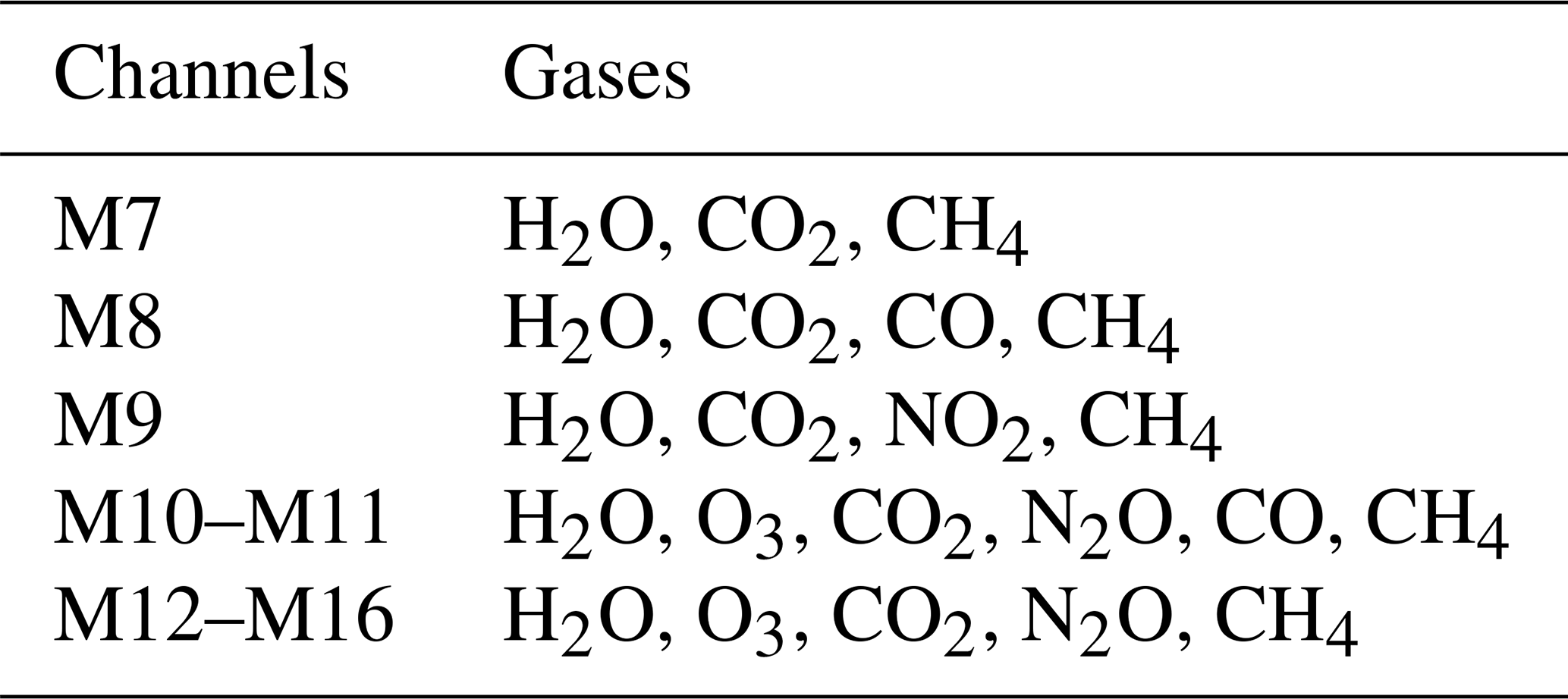
For training the RTTOV parametrizations and the proposed sparse variants, six variable gases are considered: H₂O, O₃, CO₂, N₂O, CO, and CH₄. The Fast-RT model can additionally consider SO₂ as a variable gas, but here it will be treated as a fixed gas among the total of 22 fixed gases considered. No distinction is made between water vapor absorption lines and continuum absorption. For the viewing angle, we consider 6 path secant angles from 1 to 2.25 with step 0.25 (from 0 to 63.61°).

4.1.1 Spectral Response Functions of VIIRS M-bands

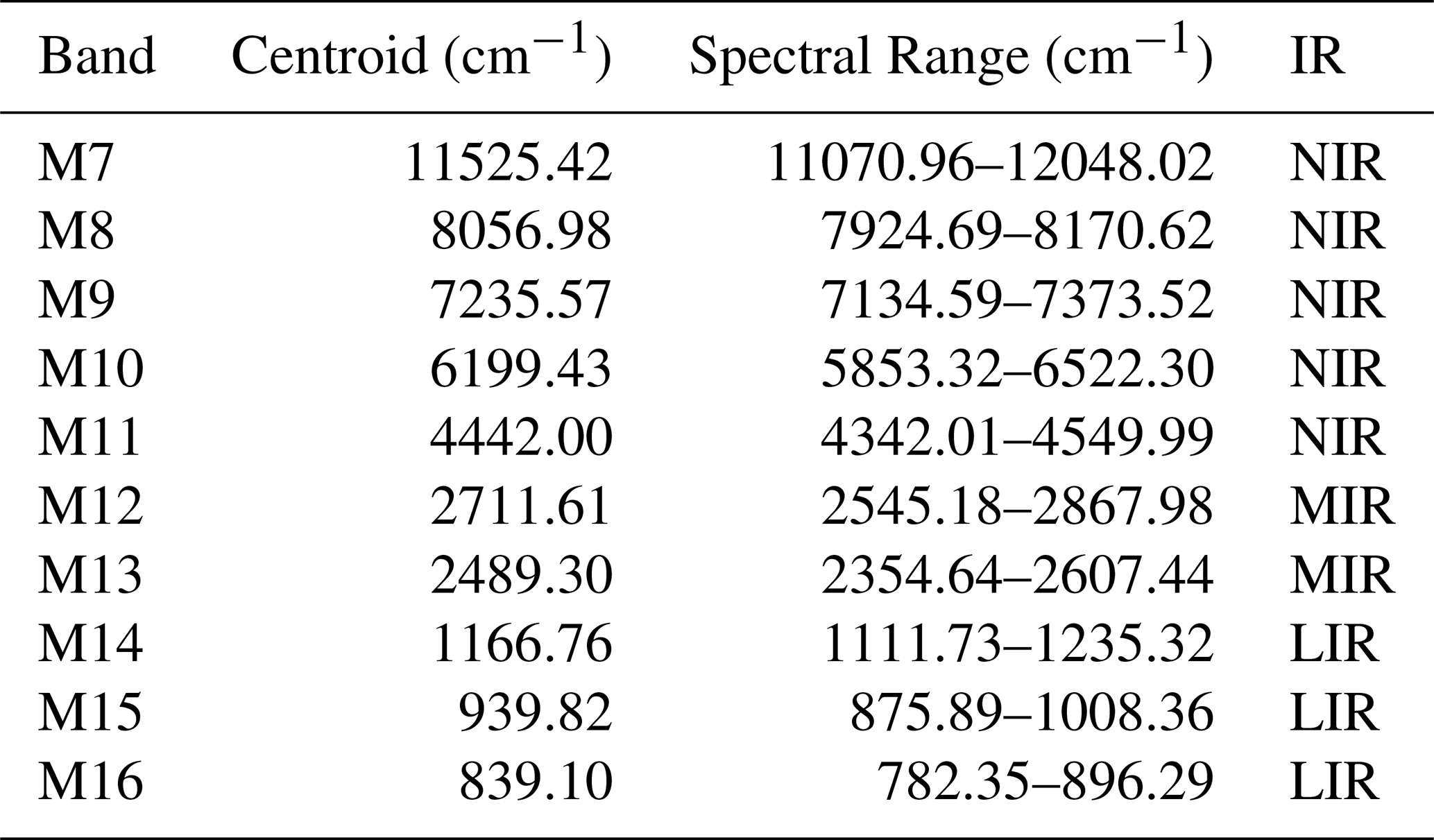
The VIIRS is an instrument on NOAA's Suomi NPP and NOAA-20 satellites, part of the Joint Polar Satellite System (JPSS). It features 16 moderate resolution bands (M-bands) that cover visible and infrared spectra. This study focuses on spectral response functions for bands M7 to M16, which cover the near (NIR), medium (MIR), and long (LIR) infrared ranges. In this study, we use the VIIRS SRF J2, which can be downloaded from the following link: https://ncc.nesdis.noaa.gov/NOAA-21/index.php (last access: 14 December 2023). Details on the centers and spectral ranges of these bands can be found in Tables 1 and 2 in Cao et al. (2017).

For each channel, the wavenumber ν and the corresponding Spectral Response Function (SRF) values are tabulated. The wavenumber tabulation typically covers a broader spectral range, denoted as [ν_a,ν_b], with noisy SRF values at the extremes of this interval. Therefore, the SRF must be truncated to a smaller interval that retains most of the relevant SRF information. Instead of using Tables 1 and 2 from Cao et al. (2017) for our calculations, we utilize channels with a spectral range broader than those. These channels are defined as $[{\mathit{\nu }}^{*}-{\mathit{\nu }}_l,{\mathit{\nu }}^{*}+{\mathit{\nu }}_u]$, where ν^* is the centroid of SRF in [ν_a,ν_b], ν_l and ν_u are the tabulated wavenumber values closest to ν^* below and above, respectively, such that the relative truncation error does not exceed $\mathit{ϵ}=\mathrm{9}\times {\mathrm{10}}^{-\mathrm{4}}$. Specifically:

$$(\mathrm{1}-\mathit{ϵ})\underset{{\mathit{\nu }}_a}{\overset{{\mathit{\nu }}_b}{\int }}\mathit{\varphi }({\mathit{\nu }}^{*},\mathit{\nu })d\mathit{\nu }\le \underset{{\mathit{\nu }}^{*}-{\mathit{\nu }}_l}{\overset{{\mathit{\nu }}^{*}+{\mathit{\nu }}_u}{\int }}\mathit{\varphi }({\mathit{\nu }}^{*},\mathit{\nu })d\mathit{\nu }.$$

The integrals are calculated using the composite trapezoidal rule. The SRF data are then truncated and normalized within this new interval, and the centroid ν^* is recalculated. The updated channels and centroids are presented in Table 1. By truncating the noisy tails of the SRF in this way, the resulting NSRF for each channel is interpolated using natural cubic splines to be used for calculating polychromatic transmittances with a much finer spectral resolution than the tabulated NSRF data. It can be shown that the error made by approximating the polychromatic transmittance with the truncated NSRF does not exceed ϵ.

Table 1 VIIRS IR M-bands (wavenumber).

4.1.2 Vertical profile database ECMWF83

For training the optical depth parametrization, we use the ECMWF83 database, which includes 83 vertical profiles with temperature and gas concentrations for H₂O, O₃, CO₂, N₂O, CO and CH₄, across 101 pressure levels, originally created to train RTTOV (Matricardi, 2008). A separate database with 22 vertical profiles covers fixed gases. These datasets are available from NWP SAF of EUMETSAT and can be downloaded at https://nwp-saf.eumetsat.int/site/ (last access: 10 November 2023).

4.1.3 Line-by-Line Transmitances with LBLRTM

In this study, LBLRTM v12.15.1 (February 2023) will be employed for Line-by-Line calculations. The software uses AER Continuum MT CKD v4.1.1. for continuum models of water vapor and other gases and the AER Line Parameter Database v3.8.1. for line parameters, which consolidates various line spectral databases, primarily HITRAN 2016 (Gordon et al., 2017).

The principal parameter in the LBLRTM calculation, to generate the optical depths for training and top-of-atmosphere radiances, are the following:

• The continuum absorption is not activated for isolated gases and fixed gases, nor when all gases are included.

• The Voigt profile is chosen for the shape of spectral lines,

• The spectral resolution is set to $d\mathit{\nu }={\overline{\mathit{\alpha }}}_{\mathit{\nu }}/\mathrm{1.5}$ where ${\overline{\mathit{\alpha }}}_{\mathit{\nu }}$ is the average value of the Voigt halfwidth for the layer. Consequently, the spectral resolution is not homogeneous across channels, achieving an average spectral resolution from $\mathrm{7.1}\times {\mathrm{10}}^{-\mathrm{3}}$ for M7 to $\mathrm{4.1}\times {\mathrm{10}}^{-\mathrm{4}}$ for M16.

• The calculation of optical depths with the software is performed only for the observation point at nadir. For other angles, variations are made directly in the calculation of polychromatic transmittances.

4.1.4 RTTOV v13 and Proposals Settings

For short, we will abbreviate Fast-RT models as follows: RTTOV13 for the standard RTTOV v13; SI for RTTOV13 with statistical threshold and ordinary least squares for parameterization; BIC+L1 for RTTOV13 with statistical threshold and BIC+LASSO regression for parameterization; and L0+L1 for RTTOV13 with statistical threshold and ℓ₀+LASSO regression for parameterization

We implemented the transmittance parametrization of RTTOV v13 as described in Saunders et al. (2020), using the same predictors, except for the method of selecting gases per channel, which is detailed below.

In RTTOV v13 in the standard form, regression parameters are obtained by including only the gases that exhibit absorption lines in each channel, as shown in Table 2. In the proposed RTTOV variants, using statistical inference and LASSO regression, all gases are included in the training.

Additionally, there are other criteria for selecting predictors in the correction term and training data by level, which are listed below:

• Threshold for gases correction term. Predictors for fixed gases are always included in the correction term. For other gases, predictors for a specific gas in a layer are included only if any of the corresponding optical depths in the training profile for that layer exceed a threshold 0.01 for CH₄ and 0.005 for the other gases. As a result, for all the VIIRS channels studied, only predictors for fixed gases and water vapor are included in the correction term.

• Threshold for Optical Depth Data Training. Optical depth data in a layer for a gas is omitted if the corresponding transmittance from the layer to the surface is less than $\mathrm{3}\times {\mathrm{10}}^{-\mathrm{6}}$. As a result, only channel M10 is affected by this selection criterion.

Table 2 Gases considered in RTTOV v13 for VIIRS M-bands.

The performance of the three proposed models, SI, BIC+L1, and L0+LASSO, is evaluated using different statistical threshold parameters ${\mathit{ϵ}}_{\mathrm{1}}\in \mathit{\{}{\mathrm{10}}^{-\mathrm{9}},{\mathrm{10}}^{-\mathrm{8}},{\mathrm{10}}^{-\mathrm{7}},{\mathrm{10}}^{-\mathrm{6}}\mathit{\}}$. Since the L0+LASSO bilevel model is based on a validation data criterion for the upper-level merit function, we split the NM data randomly in half, using one half for training the LASSO problems and the other half as validation data for evaluating model quality using the ℓ₀ regression.

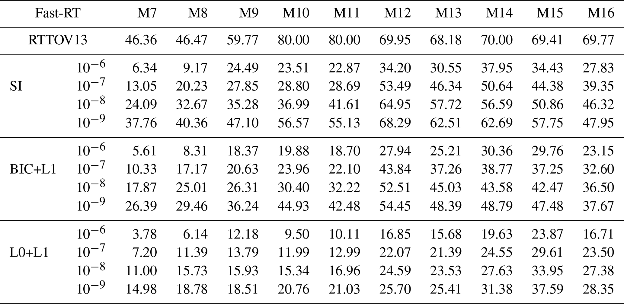
Table 3 Percentage of nonzero parameters in RTTOV v13 for each channel, for the standard configuration, SI with OLS regression, BIC+LASSO regression, and ℓ₀+LASSO regression. The second column represents the different statistical thresholds ϵ₁ used for the proposed RTTOV v13 variants.

4.2 Sparsity Pattern in the parametrization of optical depths

Table 3 summarizes the percentage of non-zero parameters (%NZ) out of a total of 11 000 parameters (worst-case scenario) for each type of optical depth model: RTTOV13, SI, BIC+L1, and L0+L1. Figures 1 and 2 show the percentage of parameter usage and computation time relative to RTTOV13. Tables 4, 5, 6, and 7 provide details on the number of non-zero parameters (NNZ) for each gas type and correction factor, for ${\mathit{ϵ}}_{\mathrm{1}}={\mathrm{10}}^{-\mathrm{6}}$.

Figure 1 Parameter usage (left) and runtime (right) of the SI method, expressed as percentages relative to those of RTTOV v13 (fixed at 100 %) for different values of ϵ₁.

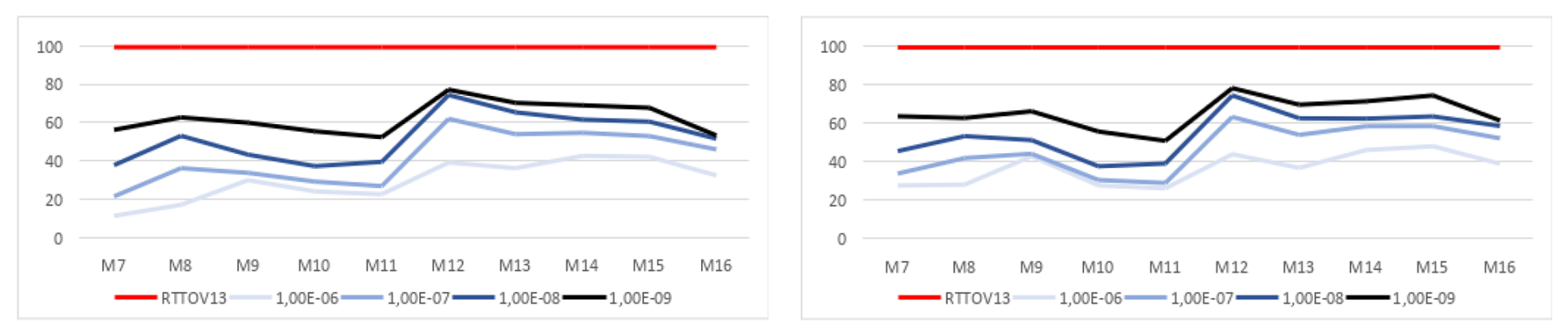
Figure 2 Parameter usage (left) and runtime (right) of the BIC+LASSO method, expressed as percentages relative to those of RTTOV v13 (fixed at 100 %) for different values of ϵ₁.

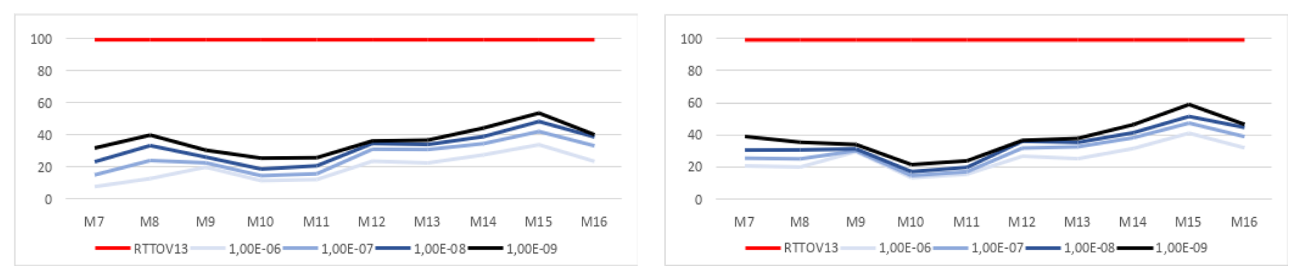
Figure 3 Parameter usage (left) and runtime (right) of the L0+LASSO method, expressed as percentages relative to those of RTTOV v13 (fixed at 100 %) for different values of ϵ₁.

In Table 3, the increase in sparsity for the proposed parametrizations compared to the general RTTOV v13 scheme is evident. RTTOV v13 induces sparsity by manually selecting gases and applying optical depth thresholds to include predictors in the correction factor. Using ${\mathit{ϵ}}_{\mathrm{1}}={\mathrm{10}}^{-\mathrm{6}}$ as a reference, in the best-case scenario with channel M7, where greater sparsity is achieved with RTTOV13, the sparsity level of RTTOV13 (53.64 %) increases to 93.66 % for SI, 94.39 % for BIC+L1, and 96.22 % for L0+L1. Conversely, in the worst-case scenario with channels M10 and M11, where RTTOV13 achieves lower sparsity (20 %), the levels increase to 76.49 % and 77.13 % for SI, 80.12 % and 81.30 % for BIC+L1, and 90.50 % and 89.89 % for L0+L1. As the statistical threshold tolerances decrease, sparsity levels also decrease; however, they remain higher than those of RTTOV13, suggesting that the computational cost benefits are preserved while achieving better sparsity results with the proposed L0+L1 model.

In Figs. 1 and 2, we present the percentage of parameter usage in the proposed optical depth approximations within RTTOV, relative to the number of parameters used in the standard RTTOV configuration, and the percentage of runtime required by the proposed schemes compared to standard RTTOV. The measured runtime corresponds to the average time of 200 evaluations of the parameterized function used to compute approximate transmittances for the 83 atmospheric profiles with 6 different viewing angles. For the following comparisons, we use ${\mathit{ϵ}}_{\mathrm{1}}={\mathrm{10}}^{-\mathrm{6}}$ as a reference. For the SI configuration, parameter usage across all channels ranges from 13.67 % to 54.21 % relative to standard RTTOV, corresponding to a runtime ranging from 29.99 % to 58.32 %; for the BIC+L1 configuration, usage ranges from 12.10 % to 43.38 %, with runtime from 26.75 % to 48.64 %; and for the L0+L1 configuration, usage ranges from 8.16 % to 34.39 %, with runtime from 13.77 % to 41.39 %. These results suggest that the computational cost of evaluating parameterized transmittances is significantly and proportionally reduced with the proposed parametrizations.

Although the absolute runtime difference is small for this limited number of profiles, in practical scenarios where transmittance functions must be evaluated for hundreds of thousands of atmospheric profiles, as required in satellite data retrieval applications, the reduction in computational time becomes highly significant for the efficiency of the retrieval process.

As an illustrative example, from Fig. 2, for channel M15, for each 100 time units required to compute transmittances with the RTTOV13 model, the L0+L1 model takes only 41.69 time units with ${\mathit{ϵ}}_{\mathrm{1}}={\mathrm{10}}^{-\mathrm{6}}$, and 59.63 time units with ${\mathit{ϵ}}_{\mathrm{1}}={\mathrm{10}}^{-\mathrm{9}}$ (worst-case), representing a significant reduction in runtime.

In Tables 5, 6, and 7, the effectiveness of introducing statistical thresholds to discard irrelevant gases by channel is evident compared to Table 4. A number of non-zero parameters below 100 for a specific gas corresponds to Case II of the statistical threshold parameterization, suggesting that the corresponding gas can be included with the fixed gases.

Table 4 Number of nonzero parameters by gas type and channel in RTTOV13.

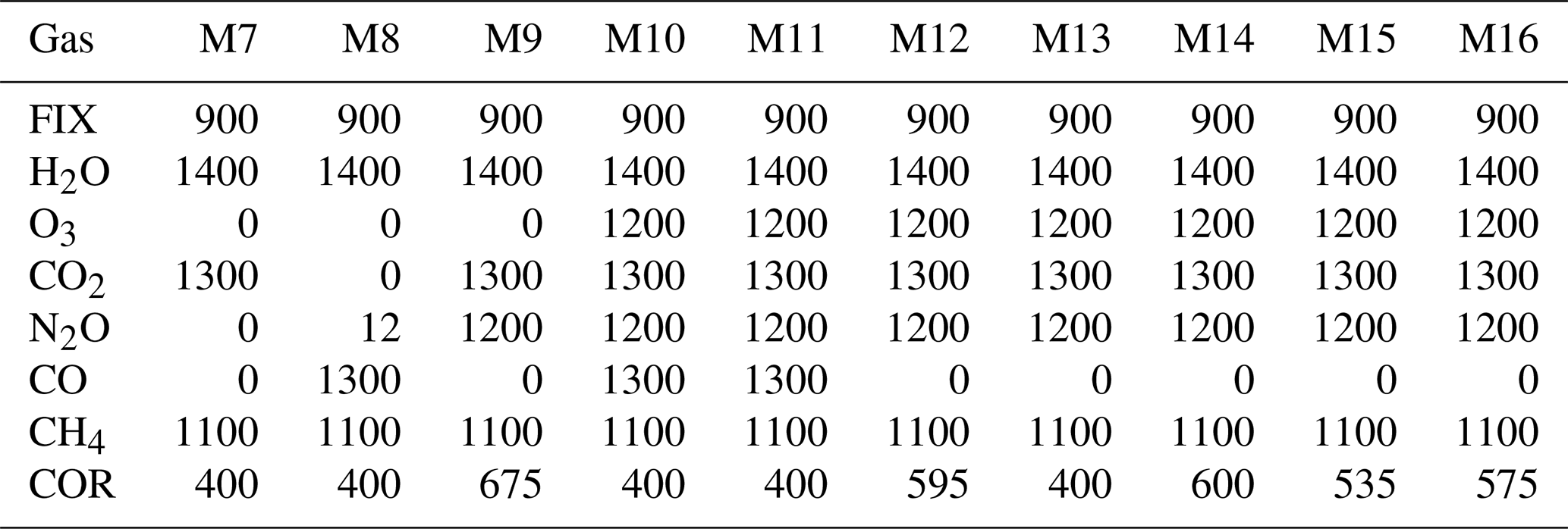
Table 5 Number of nonzero parameters by gas type and channel in SI for ${\mathit{ϵ}}_{\mathrm{1}}={\mathrm{10}}^{-\mathrm{6}}$.

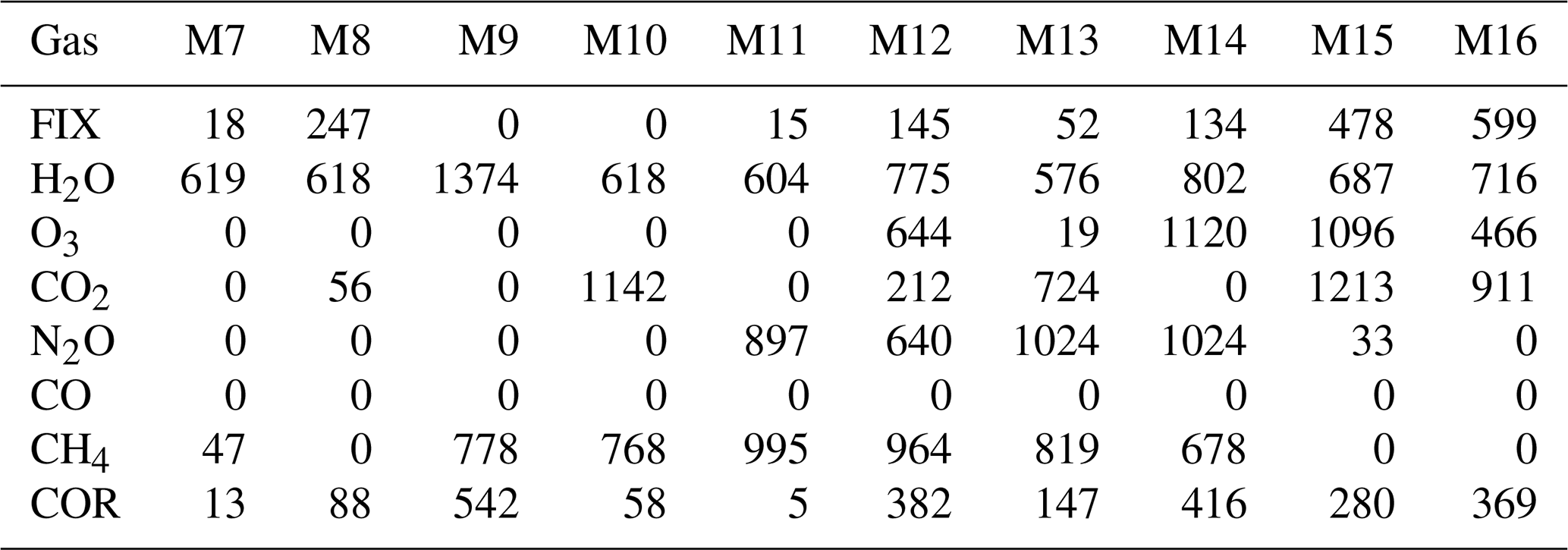
Table 6 Number of nonzero parameters by gas type and channel in BIC+L1 for ${\mathit{ϵ}}_{\mathrm{1}}={\mathrm{10}}^{-\mathrm{6}}$.

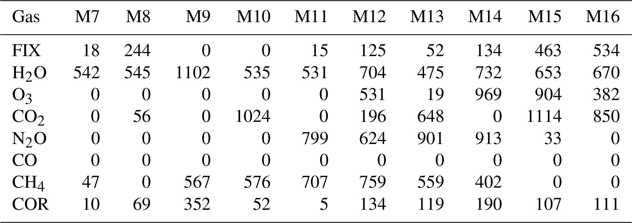
Table 7 Number of nonzero parameters by gas type and channel in L0+L1 for ${\mathit{ϵ}}_{\mathrm{1}}={\mathrm{10}}^{-\mathrm{6}}$.

To illustrate in more detail, we reference channels M11 and M12 and compare the sparsity patterns in Figs. 4 and 5 among the four parameterizations using ${\mathit{ϵ}}_{\mathrm{1}}={\mathrm{10}}^{-\mathrm{6}}$ as a reference. For the L0+L1 model and the remaining channels, see Appendix A, Figs. A1 and A2. The numbering of predictors and correctors follows RTTOV v13 (Saunders et al., 2020), see Appendix B, except for predictor 0, which corresponds to the predictor in Case II of the statistical inference proposal. Each column represents the parameters of a predictor for each pressure level, and each point in a column represents a non-zero parameter associated with that predictor at the corresponding pressure level.

For channel M11 with SI model (upper-middle Fig. 4), gases O₃, CO₂, and CO are automatically discarded, and fixed gases only need one predictor. Meanwhile, gases H₂O, N₂O, and CH₄ exhibit block-like sparsity patterns from surface pressure approximately to 200, 19, and 0.8 hPa, respectively, where concentrations of these gases are important and cause significant radiance absorption. For these gases with block-like sparsity patterns, replacing classical linear regression with L0+LASSO regression (bottom figure) clearly discards some predictors across all levels or shows them as less relevant, as seen in the sparsity patterns for CH₄ and N₂O. However, H₂O still shows sparsity, but it is difficult for this channel to determine if any predictor can be discarded at all levels due to the importance of this gas and the strong non-linear relationship among the secant angle, temperature, and gas concentration in the predictors defined for it. Using BIC+LASSO regression (lower-middle figure) highlights less relevant predictors for CH₄, but does not entirely discard it or any other gas predictor retained in the SI model. For the proposed models, no correction term is needed at all, showing that a good fit of the total transmittance is obtained by considering only the approximation of the individual gas transmittances.

For channel M12 with SI model (upper-middle Fig. 4), only CO is automatically discarded, which is expected since this gas has no absorption lines in this channel. The SI model still clearly reveals the block-like sparsity patterns of predictors and correctors for each gas at the pressure levels where they contribute to absorption (upper-middle figure). From the figure, CO₂ appears to be relevant at high pressures, approximately above 767 hPa, while O₃ seems relevant between about 2 and 260 hPa. Using L0+LASSO regression (bottom figure) for these important pressure levels demonstrates that some predictors can be entirely discarded or downweighted, as seen for fixed gases, O₃, N₂O, and CH₄. Similarly, the BIC+L1 model (lower-middle figure) highlights less relevant predictors but does not completely discard any predictor retained in the SI model, except in the corrector terms.

A similar analysis can be performed for each channel, as shown in the appendix, where Figs. A1 and A2 display the sparsity patterns for all channels using the L0+L1 model. These figures clearly indicate which gases are relevant in each channel, the pressure level ranges where they play a significant role, and which predictors are most important for reconstructing the transmittance of each gas.

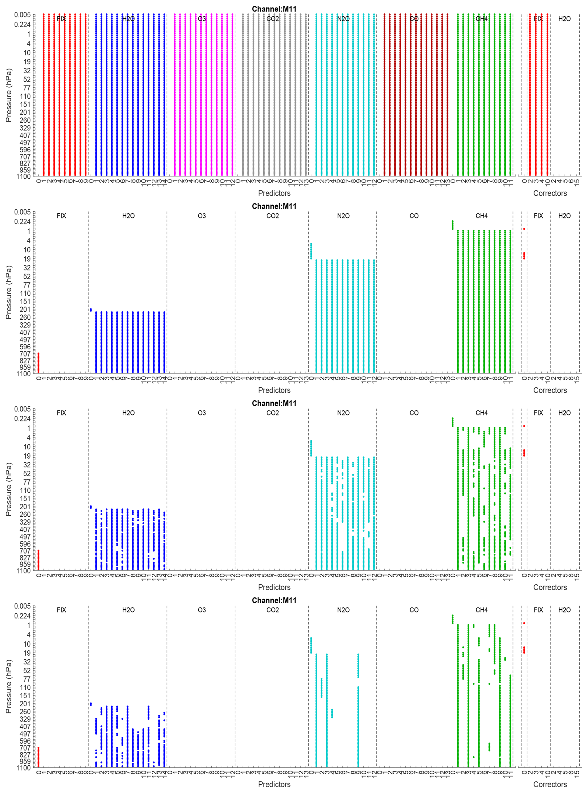
Figure 4 Sparsity pattern for channel M11, comparing RTTOV13 (Top), SI (Upper-middle), BIC+L1 (Lower-middle), L0+L1 (Bottom) for ${\mathit{ϵ}}_{\mathrm{1}}={\mathrm{10}}^{-\mathrm{6}}$.

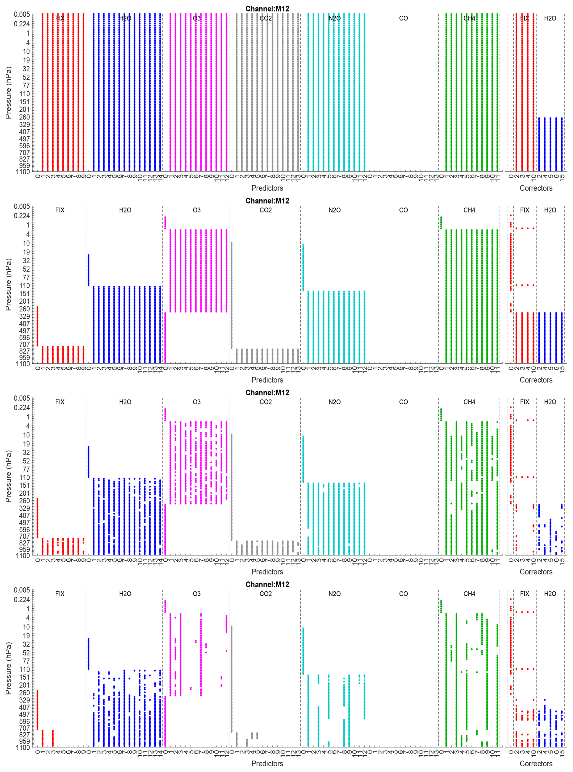
Figure 5 Sparsity pattern for channel M12, comparing RTTOV13 (Top), SI (Upper-middle), BIC+L1 (Lower-middle), L0+L1 (Bottom) for ${\mathit{ϵ}}_{\mathrm{1}}={\mathrm{10}}^{-\mathrm{6}}$.

4.3 Validation of transmittances

To validate the proposed RTTOV v13 variants, we calculated the root mean square error (RMSE) of the total transmittance for all atmospheric layers, vertical profiles, and viewing angles, as shown in the following formula:

$$\text{RMSE}={\left({\displaystyle \frac{\mathrm{1}}{LMN}}\sum _{i=\mathrm{1}}^L\sum _{j=\mathrm{1}}^M\sum _{k=\mathrm{1}}^N{\left({\mathit{\tau }}_{ijk}^{\mathrm{TOT}}-{\stackrel{\mathrm{̃}}{\mathit{\tau }}}_{ijk}^{\mathrm{TOT}}\right)}^{\mathrm{2}}\right)}^{\frac{\mathrm{1}}{\mathrm{2}}},$$

where L=100, M=83, and N=6. Here, ${\mathit{\tau }}_{ijk}^{\mathrm{TOT}}$ and ${\stackrel{\mathrm{̃}}{\mathit{\tau }}}_{ijk}^{\mathrm{TOT}}$ represent the polychromatic transmittances calculated using LBLRTM optical depths and their corresponding approximations obtained from Eq. (10) using the training data. The results are shown in Table 8. The values in the table correspond to RMSE×10⁴.

Table 8 RMSE of total transmittance for each channel, scaled by 10⁴, for the proposed RTTOV v13 variants. The second column indicates the statistical threshold ϵ₁ used for each variant.

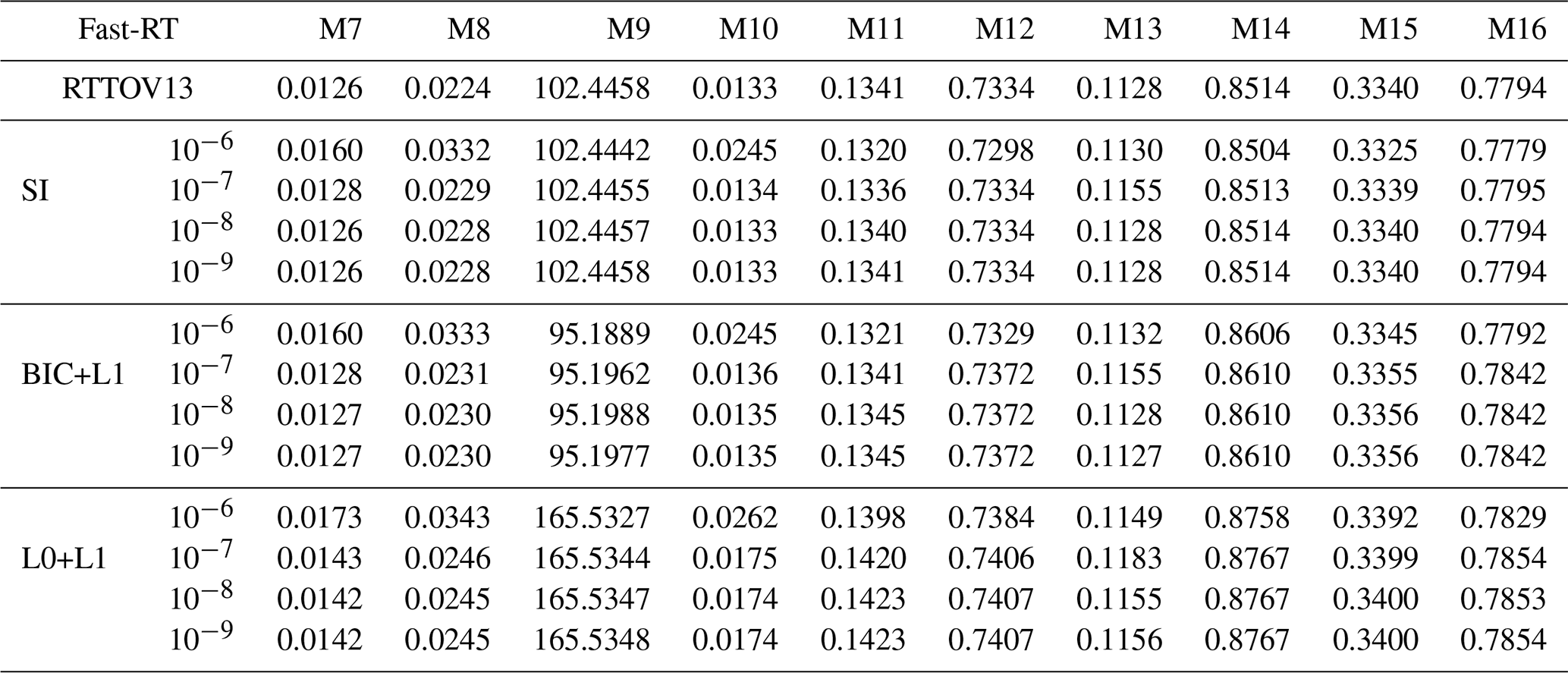
In Table 8, the RMSE for transmittance errors generally ranges between O(10⁻⁶) and O(10⁻⁵) across all Fast-RT methods and channels, except for channel M9, where errors are larger, in the range O(10⁻²) to O(10⁻³). All three proposed models slightly degrade the precision of RTTOV13, but this degradation diminishes as the statistical threshold decreases. Comparing RTTOV13 with the SI model, the error difference reduces from O(10⁻⁷) to O(10⁻⁹) on average across channels, again except for M9. With BIC+LASSO, the difference remains around O(10⁻⁷), while for channel M9 it is O(10⁻⁴). Similarly, with L0+L1 the difference is about O(10⁻⁷) for most channels, but O(10⁻³) for M9. Among the three, the L0+L1 model shows the lowest precision, as expected due to its more aggressive sparsity, yet the errors remain comparable in order of magnitude to RTTOV13.

Overall, these results indicate that including statistical thresholds in RTTOV v13 has minimal impact on the transmittance approximation. Values remain very close to the standard RTTOV13 configuration for statistical threshold tolerances below 10⁻⁶ (Table 8). Combining thresholds with LASSO regression in a bilevel framework for parameter selection, using either BIC-based or ℓ₀-regularization, slightly modifies the approximation, improving or worsening it, but variations remain small. The approximated transmittances closely match those from LBLRTM, with the added benefit of a significant runtime reduction.

4.4 Validation of brightness temperatures

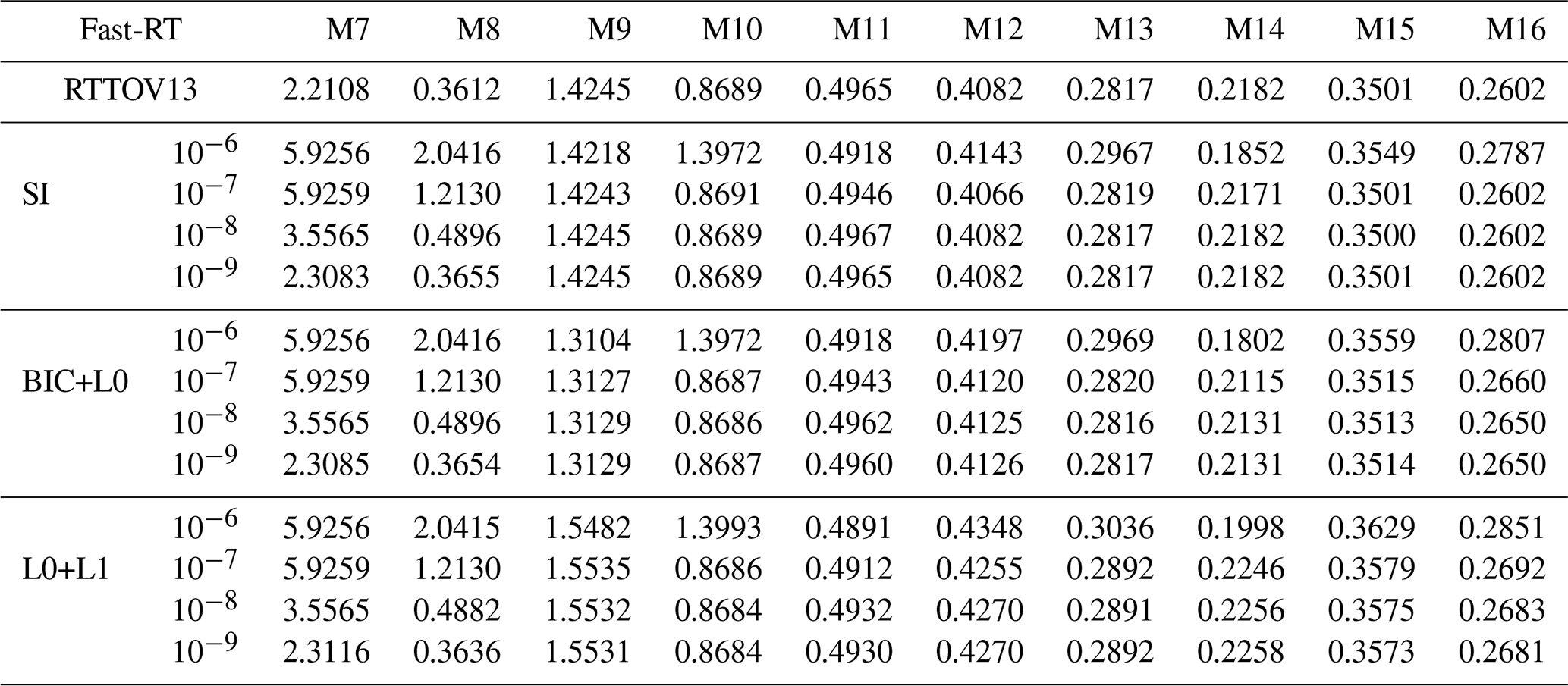
To achieve a higher level of validation for the proposed transmittance parametrization, the brightness temperatures of the profiles used for training are calculated. The approximated brightness temperatures at the top of the atmosphere were calculated using polychromatic radiances from Eq. (3), applying the approximate transmittances provided by the RTTOV v13 scheme and the proposed variants, separately. To compare these results, brightness temperatures at the top of the atmosphere were calculated using the polychromatic radiances with Eq. (2), using the monochromatic radiances calculated with LBLRTM. In all cases, the integrals were approximated using composite trapezoidal formulas, with the spacing determined by the pressure levels of the data. In each case, the resulting brightness temperatures were averaged over all profiles and viewing angles. The relative errors in BT obtained with the Fast-RT models and those obtained with LBLRTM were then calculated, which are shown in Table 9 (×10⁴). The maximum relative error for brightness temperature, determined for each profile and viewing angle, is presented in Table 10 (×10³).

Table 9 Average Relative Errors in Brightness Temperature (K), scaled by 10⁴, between the Fast-RT and LBLRTM models. The second column indicates the statistical threshold ϵ₁ used for each variant.

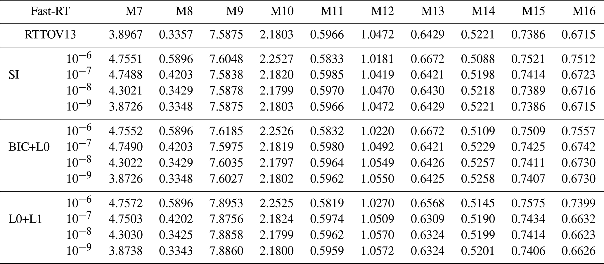
Table 10 Maximum Relative Errors in Brightness Temperature (K), scaled by 10³, between the Fast-RT and LBLRTM models. The second column indicates the statistical threshold ϵ₁ used for each variant.

In Table 9, a similar behavior is observed in the errors when approximating transmittances. The average relative error of brightness temperature generally ranges from O(10⁻⁵) to O(10⁻⁴) across all channels and Fast-RT methods. The order of magnitude of the average relative error remains consistent when comparing the four methods by channel. The differences in average relative BT errors between RTTOV13 and the SI model decrease from O(10⁻⁵) to O(10⁻⁷) when lowering the statistical threshold tolerance. Similarly, the differences between RTTOV13 and the BIC+L1 model decrease in the same manner. For the L0+L1 model, the differences decrease from O(10⁻⁵) to O(10⁻⁶).

Turning to the maximum errors, for all channels the sparse approximations of optical depth for RTTOV13 show minimal deviation from the BT results of standard RTTOV13 when ${\mathit{ϵ}}_{\mathrm{1}}\le {\mathrm{10}}^{-\mathrm{7}}$. Table 10 shows maximum relative BT errors ranging from O(10⁻⁴) to O(10⁻³) across all channels and Fast-RT methods. Comparing the maximum absolute error by channel for the four methods, errors remain of the same order of magnitude for M7, M9, and M11–M16 (${\mathit{ϵ}}_{\mathrm{1}}\le {\mathrm{10}}^{-\mathrm{6}}$), M8 (${\mathit{ϵ}}_{\mathrm{1}}\le {\mathrm{10}}^{-\mathrm{8}}$), and M10 (${\mathit{ϵ}}_{\mathrm{1}}\le {\mathrm{10}}^{-\mathrm{7}}$); in other cases, standard RTTOV13 may yield up to one order of magnitude lower errors.

Observe in Table 9 that, for some channels, the errors with the proposed methods are slightly lower than those of RTTOV13. With the L0+L1 model at ${\mathit{ϵ}}_{\mathrm{1}}={\mathrm{10}}^{-\mathrm{9}}$ this happens for channels M7, M8, M10, M11, M13, M14, and M16, and with the BIC+L1 model at the same tolerance for channels M7, M8, M10, M11, and M13. Also note that, although the BIC+L1 model gives a better transmittance fit than RTTOV13 for channel M9, its brightness temperature error is not improved. These findings suggest that using merit functions based on radiances or BT, together with model complexity penalization, instead of relying only on optical depth fitting, could improve the results of Fast-RT models within the RTTOV13 framework.

Figure 6 (left) shows the average absolute BT error between the LBLRTM model and the Fast-RT models for ${\mathit{ϵ}}_{\mathrm{1}}={\mathrm{10}}^{-\mathrm{6}}$, while Fig. 6 (right) shows the maximum absolute error across all profiles and viewing angles. The average brightness temperature shows some degradation in the proposed methods compared to RTTOV v13: in the worst case, 0.021 K for M7, 0.008 K for M8, 0.20 K for M9, while the other channels remain below 0.003 K for all proposals. For the maximum absolute error per profile and viewing angle, the worst cases are 0.961 K for M7, 0.405 K for M8, and 0.375 K for M9, with the other channels below 0.15 K. These variations are not significant in relative terms, as shown in Table 9, and decrease with a lower statistical threshold, illustrated in Fig. 7 for ${\mathit{ϵ}}_{\mathrm{1}}={\mathrm{10}}^{-\mathrm{9}}$. Under this setting, the average BT error worsens by only $\mathrm{5.7}\times {\mathrm{10}}^{-\mathrm{4}}$ K for M7, $\mathrm{3.7}\times {\mathrm{10}}^{-\mathrm{5}}$ K for M8, and $\mathrm{7.5}\times {\mathrm{10}}^{-\mathrm{3}}$ K for M9, while the others remain below $\mathrm{3.2}\times {\mathrm{10}}^{-\mathrm{4}}$ K. The maximum error increases by $\mathrm{2.1}\times {\mathrm{10}}^{-\mathrm{2}}$ K for M7, $\mathrm{1.0}\times {\mathrm{10}}^{-\mathrm{3}}$ K for M8, and $\mathrm{1.0}\times {\mathrm{10}}^{-\mathrm{3}}$ K for M9, with the other channels remaining below $\mathrm{1.5}\times {\mathrm{10}}^{-\mathrm{3}}$ K.

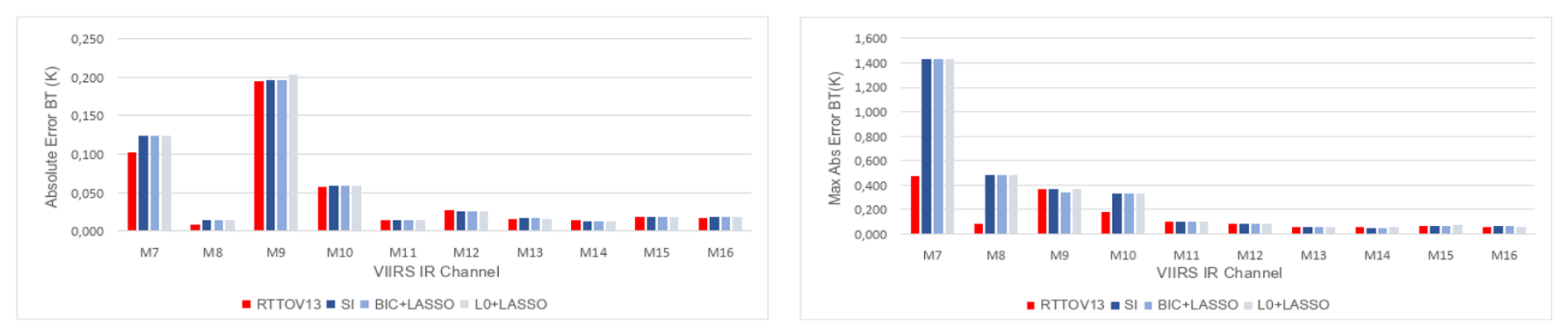
Figure 6 Average Absolute Errors (left) and Maximum Absolute Errors (right) in Brightness Temperature (K) between the Fast-RT and LBLRTM models for ${\mathit{ϵ}}_{\mathrm{1}}={\mathrm{10}}^{-\mathrm{6}}$.

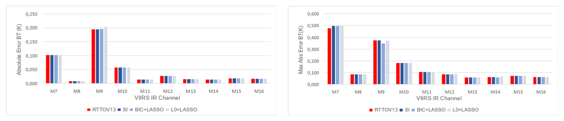
Figure 7 Average Absolute Errors (left) and Maximum Absolute Errors (right) in Brightness Temperature (K) between the Fast-RT and LBLRTM models for ${\mathit{ϵ}}_{\mathrm{1}}={\mathrm{10}}^{-\mathrm{9}}$.

These findings confirm that the proposed methods achieve an accuracy level comparable to RTTOV v13 across most channels, with only minimal degradation observed in a few cases under stringent statistical threshold tolerances.

4.5 Validation of Brightness Temperature Against Instrument Noise Characteristics

To evaluate the accuracy of the Fast RT model, we compare the brightness temperatures it generates with those from high-fidelity simulations using LBLRTM. A standard validation criterion requires that the absolute difference in brightness temperature remains below the instrument's noise level (Garand et al., 2001). Specifically, this involves comparing against the Noise Equivalent Delta Temperature (NEdT) for the thermal emissive bands (M12 to M16), and against the Noise Equivalent Delta Radiance (NEdR) for the solar reflective bands (M7 to M11). For the VIIRS M-bands, Table 11 presents the NEdT values and the signal-to-noise ratios (SNR) used to compute the corresponding NEdR values, as reported in Table 1 of the manual Cao et al. (2017).

Table 11 SNR and NEdT Values for VIIRS IR M-Bands (L: Low Gain Mode, H: High Gain Mode).

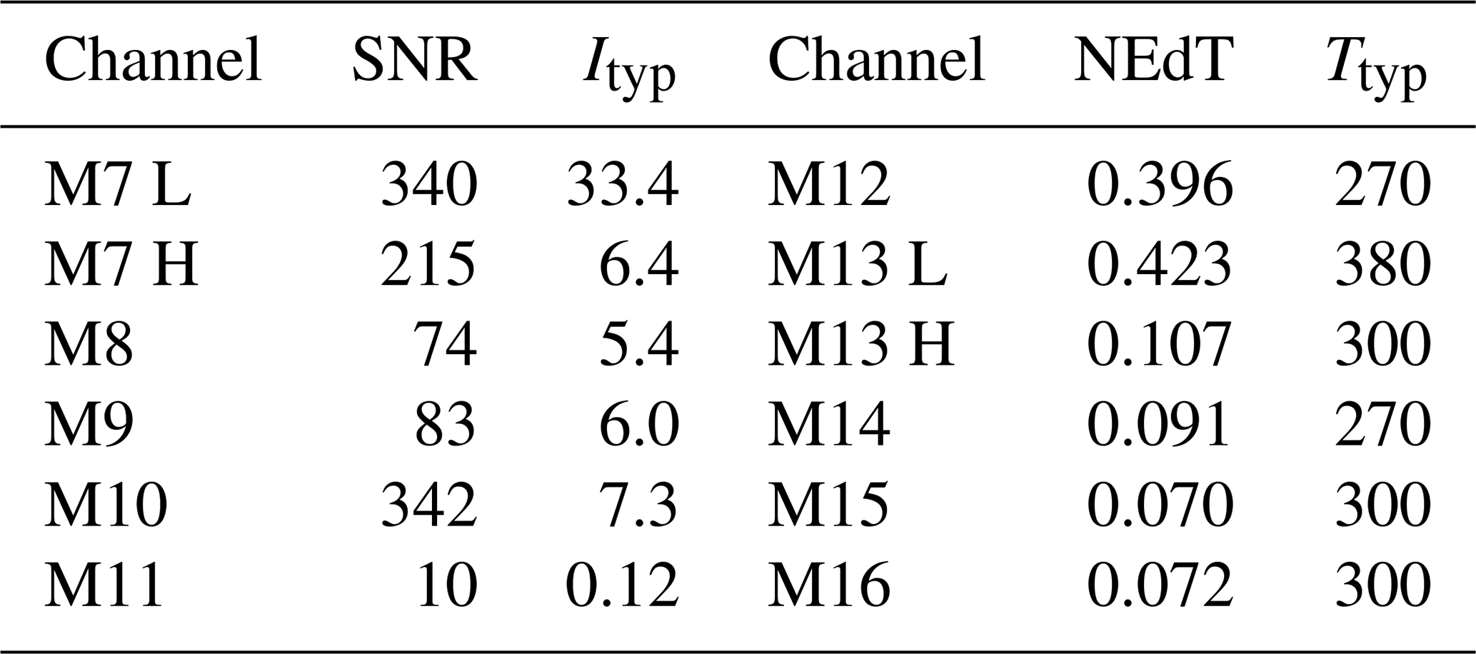
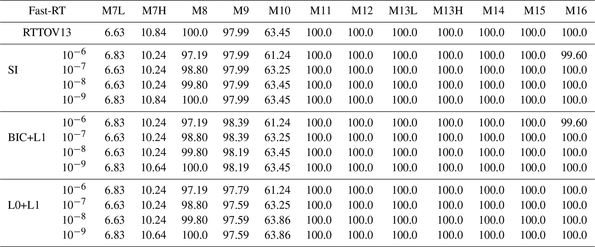
Table 12 Percentage of absolute differences in radiance below the NEdR threshold for channels M7–M11, and percentage of absolute differences in brightness temperature below the NEdT threshold for channels M12–M16. The second column indicates the statistical threshold ϵ₁ used for each variant.

For each channel from M7 to M11, the table reports the SNR at the reference radiance I_typ (W m⁻² sr⁻¹ µm⁻¹), and for channels M12 to M16, it reports the NEdT at the reference temperature T_typ (K). For a thermal emissive band, the NEdT at temperature T is defined as

$$\text{NEdT}\left(T\right)=\text{NEdT}\left(T_{\text{typ}}\right)\cdot {\displaystyle \frac{B^{\prime }\left(T_{\text{typ}}\right)}{B^{\prime }\left(T\right)}}$$

where B^′ is the derivative of the Planck function with respect to temperature. For solar reflective bands, the Noise Equivalent Delta Radiance (NEdR) at radiance I is defined as

$$\text{NEdR}\left(I\right)={\displaystyle \frac{I}{\text{SNR}}}.$$

Let I_ij and ${\stackrel{\mathrm{̃}}{I}}_{ij}$ denote the top of atmosphere polychromatic radiances obtained using LBLRTM and the Fast RT model, respectively, for atmospheric profile i and observation angle θ_j, and let T_ij and ${\stackrel{\mathrm{̃}}{T}}_{ij}$ be the corresponding brightness temperatures. For emissive bands, the following condition must be satisfied:

$$|T_{ij}-{\stackrel{\mathrm{̃}}{T}}_{ij}|\le \text{NEdT}\left(T_{ij}\right),$$

and for solar reflective bands, we require:

$$|I_{ij}-{\stackrel{\mathrm{̃}}{I}}_{ij}|\le \text{NEdR}\left(I_{ij}\right).$$

The percentage of atmospheric profiles for which these conditions are satisfied serves as a practical metric to evaluate the quality of the forward model. A high proportion of cases meeting the criterion indicates that the modeling error is smaller than the instrument noise, ensuring that the simulated radiances are sufficiently accurate for satellite retrievals and potentially suitable for data assimilation. Table 12 reports the percentage of cases, computed over 83 atmospheric profiles and 6 viewing angles, for which the corresponding noise threshold condition is met.

In the Table 12, it can be observed that for channels M11 to M16, all methods fully satisfy the noise condition, and the proposed methods are comparable to standard RTTOV13 for a statistical tolerance threshold of ${\mathit{ϵ}}_{\mathrm{1}}\le {\mathrm{10}}^{-\mathrm{6}}$. For channels M7 to M10, a stricter statistical tolerance threshold is required to achieve percentages comparable to RTTOV13. For channels M7 and M10, the fulfillment of the noise criterion is quite poor; we infer that this is due to the lack of solar radiation inclusion in the various Fast-RT methods. However, the results obtained with the proposed methods are similar to RTTOV13 for small statistical thresholds. For channel M9, the proposed BIC+L1 model slightly improve the percentage of profiles that meet the noise threshold compared to standard RTTOV13. It is clear that the proposed methods reproduce the results of standard RTTOV13 for large statistical thresholds in the emissive bands and for smaller statistical thresholds in the solar reflective bands, while offering the advantage of greater computational efficiency due to the induced sparsity.

5 Conclusions

This study presents an automatic and sparse optical depth parametrization method for the RTTOV v13 model, aimed at optimizing parameter adjustment. The method applies statistical thresholding across different pressure levels, followed by LASSO regression, instead of the traditional least squares approach in the RTTOV v13 framework. A bilevel optimization approach is used to select the optimal regularization parameter, employing different model validation criteria: one based on ℓ₀ regression and another on the Bayesian Information Criterion (BIC). These alternatives enforce significant sparsity across all optical depth regression parameters, substantially reducing the computational cost of the Fast-RT model without compromising accuracy.

Validation experiments were conducted on the infrared channels of the M-bands for the VIIRS instrument. Different validation criteria were considered, including transmitance fitting against LBLRTM transmitance, brightness temperature fitting against LBLRTM transmitance, and the difference between brightness temperature and the instrument's Noise Equivalent Delta Temperature. The results show consistency with RTTOV v13, while providing improved runtime performance in the evaluation of parameterized transmitances.

The induced sparsity automatically excludes gases with negligible absorptivity in a channel, identifies pressure levels where gases significantly absorb radiance, highlights the most relevant predictors for each gas type, and classifies gases as either fixed or variable. This technique is particularly advantageous for multispectral instruments where multiple gases exhibit strong correlations in radiance absorption, especially in large-scale variable retrievals for inverse problems. The proposed method may be extended to other Fast-RT models, such as CRTM, and to other satellite instruments, such as the Advanced Technology Microwave Sounder (ATMS) and the Cross-track Infrared Sounder (CrIS), to enhance both the computational efficiency of radiative transfer models and the accuracy of retrieved atmospheric profiles. The numerical results obtained at different levels of validation, particularly the output from the proposed model indicating a high proportion of profiles with errors below the instrument's NEdT, provide strong evidence of its suitability and potential for satellite data assimilation. Nevertheless, applying sparsity-inducing models in this context requires a careful evaluation of the sensitivity of simulated radiances to the underlying model state variables. This evaluation, in practical scenarios such as the satellite data assimilation of radiances from the proposed Fast-RT model, will be carried out in future work.

Additionally, future directions may include a benchmark comparison against other existing Fast-RT models and more general scenarios with extreme atmospheric conditions, considering strong absorption due to extreme pollution events and incorporating variable SO₂ concentrations in environments with high volcanic activity.

Appendix A: Sparsity Pattern for RTTOV13+SI+LASSO

Figure A1 Sparsity pattern for channels M7 to M11 in L0–L1 for ${\mathit{ϵ}}_{\mathrm{1}}={\mathrm{10}}^{-\mathrm{6}}$.

Figure A2 Sparsity pattern for channels M13 to M16 in L0–L1 for ${\mathit{ϵ}}_{\mathrm{1}}={\mathrm{10}}^{-\mathrm{6}}$.

Appendix B: RTTOV v3 Predictors

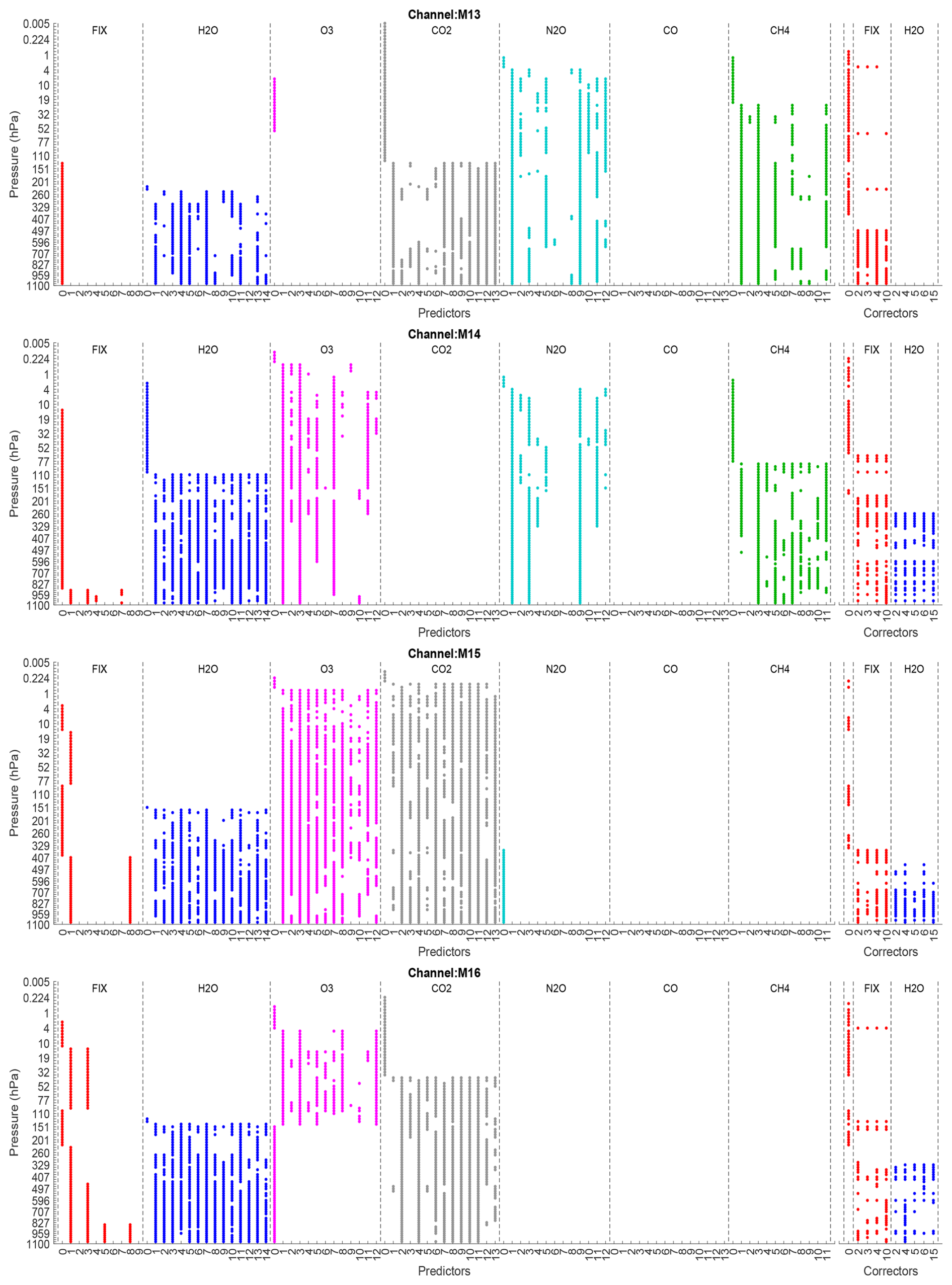
Table B1 Predictors for RTTOV v13, (Saunders et al., 2017). ^* Not an original RTTOV v13 predictor; this predictor corresponds to Case II of the statistical threshold parametrization.

$p\mathit{\delta }p\left(l\right)=p(l+\mathrm{1})\left(p\right(l+\mathrm{1})-p(l\left)\right)$,	$p\mathit{\delta }p\left(\mathrm{0}\right)=p\left(\mathrm{1}\right)\left(p\right(\mathrm{2})-p(\mathrm{1}\left)\right)$,
$T\left(l\right)={\displaystyle \frac{\mathrm{1}}{\mathrm{2}}}\left(T^{\text{prof}}\right(l)+T^{\text{prof}}(l+\mathrm{1}\left)\right)$,	$T^{*}\left(l\right)={\displaystyle \frac{\mathrm{1}}{\mathrm{2}}}\left(T^{\text{ref}}\right(l)+T^{\text{ref}}(l+\mathrm{1}\left)\right)$,	$T_r\left(l\right)={\displaystyle \frac{T\left(l\right)}{T^{*}\left(l\right)}}$,
$T_w\left(l\right)={\displaystyle \frac{{\sum }_{i=\mathrm{1}}^{l}p\mathit{\delta }p(l-\mathrm{1})T\left(l\right)}{{\sum }_{i=\mathrm{1}}^{l}p\mathit{\delta }p(l-\mathrm{1})T^{*}\left(l\right)}}$,	$\mathit{\delta }T\left(l\right)=T\left(l\right)-T^{*}\left(l\right)$,
$G\left(l\right)={\displaystyle \frac{\mathrm{1}}{\mathrm{2}}}\left(G^{\text{prof}}\right(l)+G^{\text{prof}}(l+\mathrm{1}\left)\right)$,	$G^{*}\left(l\right)={\displaystyle \frac{\mathrm{1}}{\mathrm{2}}}\left(G^{\text{ref}}\right(l)+G^{\text{ref}}(l+\mathrm{1}\left)\right)$,	$G_r\left(l\right)={\displaystyle \frac{G\left(l\right)}{G^{*}\left(l\right)}}$,
$G_w\left(l\right)={\displaystyle \frac{{\sum }_{i=\mathrm{1}}^{l}p\mathit{\delta }p(l-\mathrm{1})G\left(l\right)}{{\sum }_{i=\mathrm{1}}^{l}p\mathit{\delta }p(l-\mathrm{1})G^{*}\left(l\right)}}$,	$G_{\mathrm{wt}}\left(l\right)={\displaystyle \frac{{\sum }_{i=\mathrm{1}}^{l}p\mathit{\delta }p(l-\mathrm{1})T\left(l\right)G\left(l\right)}{{\sum }_{i=\mathrm{1}}^{l}p\mathit{\delta }p(l-\mathrm{1})T^{*}\left(l\right)G^{*}\left(l\right)}}$.

where p(l) is the pressure (hPa) at level l, T^prof(l) is the temperature (K) at level l of the input profile, T^ref(l) is the temperature (K) at level l of the reference profile which is the mean over the training profile set, $G\in \mathit{\{}W={\mathrm{H}}_{\mathrm{2}}\mathrm{O},{\mathrm{O}}_{\mathrm{3}},{\mathrm{CO}}_{\mathrm{2}},{\mathrm{N}}_{\mathrm{2}}\mathrm{O},\mathrm{CO},{\mathrm{CH}}_{\mathrm{4}}\mathit{\}}$ represents gas concentration (ppmv over dry air), G^prof(l) are the gas concentrations at level l of the input profile and G^ref(l) are the gas concentrations at level l of the reference profile which is the mean over the training profile set.