The spatial distribution of convective precipitation – an evaluation of cloud microphysics schemes with polarimetric radar observations

The representation of cloud microphysics in numerical weather prediction models contributes significantly to the uncertainty of weather forecasts. Polarimetric radar observations are increasingly used to evaluate numerical weather simulations, due to their sensitivity to microphysical properties. Typically, this evaluation is performed for individual case studies, which limits the generalizability of the results. This is particularly problematic for convective precipitation events, which are characterized by high variability due to their small scale and rapid error growth of initial uncertainties, and are often associated with severe weather phenomena. In this study, the performance of microphysics schemes in the simulation of convective precipitation events is evaluated statistically over a 30 d dataset. The aim is to assess the distribution of precipitation into convective and stratiform regions, and the microphysical properties in these regions based on radar reflectivity and differential reflectivity. Within a Weather Research and Forecasting model setup, 5 different microphysics schemes of varying complexity are evaluated. The choice of microphysics schemes has a significant impact on the distribution of precipitation; the median convective area fraction varies by an order of magnitude between the microphysics schemes. These differences are attributed to differences in rain drop size distributions. In the convective core, the FSBM and Morrison schemes frequently lack large rain drops, while the Thompson and P3 schemes simulate too many. Statistical evaluations are important to address the prevailing uncertainty surrounding cloud microphysics. The framework presented in this study can serve as a guide for future statistical evaluations of weather models with polarimetric radar observations.

1 Introduction

Simulation of convective precipitation events presents a particular challenge, owing to their small scale and rapid error growth of initial uncertainties (Selz and Craig, 2015; Hohenegger and Schär, 2007). These events are characterized by strong vertical air motions, and a high spatial variability (Powell et al., 2016) and frequently coincide with severe weather phenomena, including flooding, hail, strong winds, and tornadoes (Doswell III, 2001). Despite of their potential for hazardousness, current numerical weather prediction models struggle to accurately predict convective precipitation events. Xue et al. (2017) for example demonstrate that 3 different microphysics schemes produce a substantially different dynamical and thermodynamical structure of a squall line over the continental United States. These events often consist of a leading convective core and a trailing stratiform region (Houze, 1994), with the convective core characterized by strong updrafts and downdrafts, intense precipitation and winds, and possibly hail. The stratiform region typically has a lower precipitation intensity, but can potentially cover larger areas. Due to the different nature and hazard of these regions, the correct representation of the distribution of precipitation into these regions is important for weather forecasting and hydrology.

The accurate simulation of the convective core and surrounding stratiform precipitation is a significant challenge for cloud microphysics schemes. For example, Shrestha et al. (2022) found that their simulations of three convective storms produced too small convective areas compared to stratiform areas. Han et al. (2019) found that their simulations of a squall line case underestimated total stratiform precipitation, primarily due to the underestimation of precipitation area. Qian et al. (2018) found that the trailing stratiform region of a simulated squall line case was strongly sensitive to the choice of cloud microphysics schemes. Not only the distribution of precipitation into convective core and trailing stratiform region is challenging, but also the representation of microphysical properties in each category. Wu et al. (2021) show that the microphysical characteristics of precipitation within a typhoon differ considerably to radar observations and are mainly determined by the microphysics scheme used. In Köcher et al. (2022), we demonstrate that some of the tested microphysics schemes produce graupel particles that are too large or too dense within convective cores. In a related study, Planche et al. (2019) examined the discrepancies between radar observations and simulations for a squall line case, highlighting differences in the vertical profile of rain size distributions within the stratiform region. These discrepancies were primarily attributed to the process of drop breakup. Sun et al. (2023) demonstrate that two evaluated microphysics schemes encounter difficulties in consistently reproducing radar signals in both, the stratiform and convective regions, as well as throughout the vertical profile. These issues are attributed to deficiencies in particle size distributions, density assumptions, and the simulation of ice processes. All of these studies underscore the prevailing uncertainty surrounding the representation of cloud microphysics in numerical weather prediction models, particularly in the context of convective precipitation events.

Cloud microphysical processes include the formation of cloud droplets, ice crystals, and precipitation (Lamb, 2003; Morrison et al., 2020). A characteristic feature of microphysical processes is its inherent complexity, involving numerous (nonlinear) interactions among diverse species of particles and the surrounding air, as well as a broad spectrum of particle shapes and sizes. Given the vast number of particles in a cloud and the complexity of the processes, direct simulation of these processes over the entire range of scales is computationally unfeasible. Consequently, these processes are typically parameterized, meaning their effects on key variables are described without explicitly calculating the processes themselves. This is typically done by so-called cloud microphysics schemes (e.g., Thompson et al., 2008; Morrison and Milbrandt, 2015; Shpund et al., 2019; Seifert and Beheng, 2005). However, uncertainties in microphysical process rates persist due to fundamental gaps in our understanding of the processes, as well as the lack of observations to constrain the schemes (Morrison et al., 2020). Constraining microphysical processes is challenging, as they occur on small scales. Observational constraints can be derived from laboratory studies (e.g., Seidel et al., 2024), in situ observations (e.g., Billault-Roux et al., 2023), and remote sensing observations (e.g., Tana et al., 2023). However, all of these approaches are limited: laboratory studies are typically limited to a small number of particles and idealized setups. In situ observations, for example with aircraft, require much effort and are spatially limited. Remote sensing observations, such as radar observations, offer much better spatial coverage. However, they generally cannot measure the microphysical properties directly. Instead, these properties are inferred from the observed signals. These limitations hinder the validation microphysics schemes to improve their representation in models.

In recent years, polarimetric radar observations have been established. For example, in 2015, the German Meteorological Service (Deutscher Wetterdienst, DWD) finished upgrading its radar network to polarimetric radars (Trömel et al., 2021). Polarimetric radars transmit a radar signal at two orthogonal polarizations, and measure the power and phase of the backscattered signals at both polarizations. The received polarimetric signals are affected by numerous particle properties, including shape, size distribution, orientation, phase, and number concentration of particles within the measurement volume. Consequently, these polarimetric fingerprints can be utilized to deduce information concerning cloud microphysical processes that affect these properties. This, in turn, can be used to constrain cloud microphysics schemes in NWP models (Kumjian, 2012; Ryzhkov et al., 2020).

Meanwhile, there are several studies that have employed polarimetric radar observations to evaluate cloud microphysics schemes in NWP models (e.g., Chen and Liu, 2024; Li et al., 2023; Chen et al., 2021; You et al., 2020; Putnam et al., 2016; Brown et al., 2016; Wu et al., 2021, and many more). However, all of these studies are limited to case studies. While case studies are instrumental to understand the processes in detail, they are limited in their generalizability. This limitation is particular problematic in the context of for convective precipitation, due to large variability between different events (Flack et al., 2019). Only few studies exist that evaluate cloud microphysics schemes statistically over a large dataset. Caine et al. (2013) statistically compared convective cell properties; however, their statistics were limited to less than 5 d. Stein et al. (2015) evaluated simulated convective storms of 40 cases, but only for one microphysics scheme and without the use of polarimetric radar observations. In Köcher et al. (2022), we provided a setup for statistical evaluation of weather model simulations with polarimetric radar measurements which was applied in Köcher et al. (2023) to statistically evaluate the performance of 5 microphysics schemes in predicting high-impact weather events, such as hail and heavy rain. Statistical analysis is not only important for representative results, but also required for uncertainty estimation. As highlighted by Morrison et al. (2020) in one of their main conclusions, the critical evaluation of model performance necessitates statistically robust remote-sensing approaches.

The objective of this study is to statistically evaluate the performance of 5 cloud microphysics schemes in simulating the distribution of precipitation into convective and stratiform regions. The aim is to assess the microphysical properties in these regions based on the observed and simulated polarimetric radar signals. Within the scope of this study, we solely focus on the differential reflectivity (Z_dr) and radar reflectivity (Z). Other polarimetric variables, such as specific differential phase (K_dp) and correlation coefficient (RHOhv) could provide further insight into the microphysical properties, but will be left for future studies.

The remainder of this paper is structured as follows: Sect. 2 describes the data and methods used in this study. Section 3 describes the results of the analysis, including the vertical distribution of reflectivity signals (Sect. 3.1), the distribution of precipitation into convective and stratiform regions (Sect. 3.2), the microphysical properties of the precipitation within these regions based on polarimetric radar statistics (Sect. 3.3), and the impact of the simulated rain drop size distributions on the polarimetric radar signals (Sect. 3.4). Section 4 provides a summary and conclusions of the study.

2 Data and methods

The data and methodologies employed in this study build upon Köcher et al. (2022). The dataset consists in total of 30 d of precipitation events in the Munich region in South Eastern Germany in 2019 and 2020. These events were observed from the German Meteorological Service (Deutscher Wetterdienst, DWD) radar network, and simulated with the Weather Research and Forecasting (WRF) model (Skamarock et al., 2019). A complete list of the measurement days is provided in Köcher et al. (2022), in their Table A1. Below, we provide a brief overview of the dataset. For a detailed description, we refer to Köcher et al. (2022).

The observational data utilized in this study was provided by the DWD, which operates a network of fully dual polarimetric C-band radars. These radars provide the polarimetric variables differential reflectivity (Z_dr), specific differential phase (K_dp), and correlation coefficient (RHOhv), in addition to the radar reflectivity (Z). In this study, we solely focus on raw Z and Z_dr data, i.e., without any attenuation correction applied. The network consists of 17 radars that cover the entire area of Germany. For the purpose of this study, the closest radar to Munich, i.e., the radar in Isen, southern Germany was selected. The operational measurement strategy of the DWD radars involve a volume scan every five minutes, which consist of Plan Posistion Indicator (PPI) scans at 11 elevation angles spanning from 0.5–25°. Further details on the DWD radar network and the measurement strategy can be found in Helmert et al. (2014).

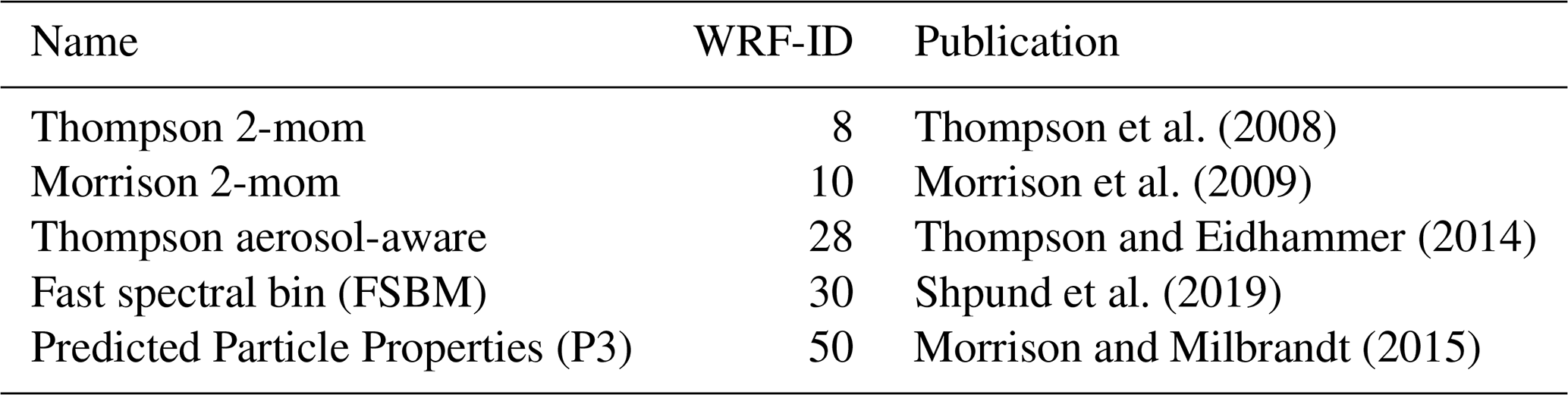
The simulations were performed using a regional limited area model setup of WRF, version 4.2. The inner nest is centered over Munich with a horizontal grid spacing of 400 m, 40 vertical levels, and a horizontal extent of 144 km×144 km. 5 microphysics schemes were are employed and listed in Table 1. The simulations were initialized with reanalysis data from the Global Forecast System (GFS; National Centers For Environmental Prediction/National Weather Service/NOAA/U.S. Department Of Commerce, 2015) at 0.25° horizontal resolution.

Thompson et al. (2008)Morrison et al. (2009)Thompson and Eidhammer (2014)Shpund et al. (2019)Morrison and Milbrandt (2015)

Table 1 Abbreviations, WRF-IDs, and corresponding publications of the employed microphysics schemes.

In this study, observed polarimetric radar signals are compared to simulated radar signals. The Cloud-resolving model Radar SIMulator (CR-SIM, version 3.33; Oue et al., 2020) is utilized to simulate the radar signals from the WRF model output. CR-SIM is based on the T-matrix method (Barber and Yeh, 1975) and is capable of providing the polarimetric variables Z_dr, K_dp, and RHOhv based on assumed particle shapes and particle orientations, depending on the simulated hydrometeor classes. The simulated particle densities and particle size distributions are consistent with the microphysics schemes employed. CR-SIM does not implement a melting scheme; instead, particles are either completely frozen or completely melted, in accordance with the microphysics schemes. This makes it impossible to simulate melting layer effects such as the “bright band” (Austin and Bemis, 1950), and hence the analysis in this study is focused on heights above and below the melting layer. Furthermore, the attenuations effects are simulated by CR-SIM and applied to the simulated reflectivity (Z) and differential reflectivity (Z_dr).

The radar data resolution depends on the distance to the radar. To ensure comparability of the datasets, both are interpolated to a joint Cartesian grid with a horizontal grid spacing of 400 m. The radar data is interpolated to the model grid using an inverse distance interpolation. To ensure a fair comparison between model and radar geometry, as well as to apply the attenuation correction, the model data is first interpolated to a radar grid. This is achieved by considering the radar beam geometry, whereby each pixel is weighted based on the distance to the radar beam center. To allow the application of a cell-tracking algorithm that operates on a Cartesian grid (see Sect. 2.1), the resulting data is then interpolated back to the Cartesian grid using the same inverse distance interpolation as for the radar data.

2.1 Cell-tracking

An automatic cell-tracking algorithm (tobac; Sokolowsky et al., 2024) is applied to the matched radar and simulation data alike to identify convective cells and their surrounding stratiform regions. Note that this approach is different from the methodology employed in our prior study (Köcher et al., 2022). In the preceding study, the focus was exclusively on convective cores. In contrast, the present study aims for a separation into convective and stratiform regions. Tobac not only tracks convective cores, but also provides the fucntionality to assign surrounding stratiform regions to the convective cores through the implementation of a segmentation processes based on a watershedding algorithm. The tobac algorithm consists of three main steps:

1. Identification of convective cells based on reflectivity thresholds. For the purpose of this study, a reflectivity threshold of 35 dBZ is used. The location of the maximum reflectivity within a cell is designated as the cell's center.

2. Segmentation of surrounding stratiform precipitation. A surrounding volume is associated with each convective cell based on watershedding with a fixed threshold of 5 and 35 dBZ for the stratiform and convective parts, respectively.

3. Tracking of cells over time. Identified cells are linked over time based on the cell position using the python library trackpy (Allan et al., 2021).

Based on the identified convective cells and the associated stratiform regions, the convective area fraction (CAF) is calculated. The CAF is defined as the ratio of the area covered by convective precipitation to the total area covered by precipitation and will be used to describe the distribution of precipitation into convective and stratiform regions. All in all, a total of 8395 convective cells were identified by the tobac algorithm over the 30 d dataset in the radar data while the number of cells in the simulations varied depending on the microphysics scheme and is discussed below. An example of the cell tracking output is shown in Fig. 1. For a more detailed description of the radar data, simulation setup, and forward operator, please refer to Köcher et al. (2022). An example case demonstrating the simulation output of the five different microphysics schemes within the NWP model setup is presented in Köcher et al. (2023).

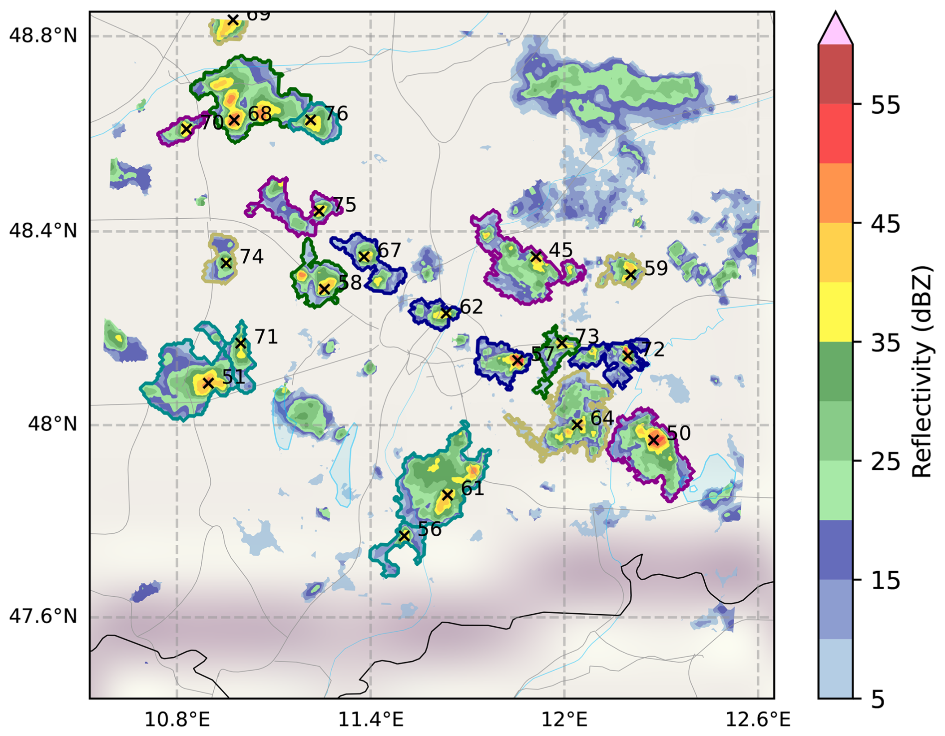
Figure 1 Example tobac tracking applied to DWD radar data on the 20 June 2020, 10:05 UTC. In color the measured reflectivity. Black “×” symbols are the identified cells and the black numbers are the corresponding cell IDs. The colored lines around the precipitation areas are the identified stratiform regions that were assigned to the convective cells. Background map data by OpenStreetMap (http://openstreetmap.org, last access: 7 April 2025; © OpenStreetMap contributors. Distributed under the Open Data Commons Open Database License (ODbL) v1.0.). Roads, rivers, and lakes made with Natural Earth (https://www.naturalearthdata.com, last access: 7 April 2025).

3 Results

In general, the majority of the weather model simulations yielded comparable total surface precipitation amounts, ranging from 295–321 mm precipitation summed over the entire 30 d over the whole domain (Fig. 2). Only the FSBM scheme yielded slightly higher total precipitation amounts, reaching 390 mm. However, while the total precipitation varies by a factor of only around 10 %–30 %, the number of identified cells varies by a factor of 2, ranging from 5261–11 576 across the microphysics schemes. This indicates differences in distribution of precipitation into convective and stratiform regions between the microphysics schemes. For example, FSBM precipitates more water than P3, but shows a much lower number of intense convective cells, indicating more wide spread and less convectively active rain weather in FSBM.

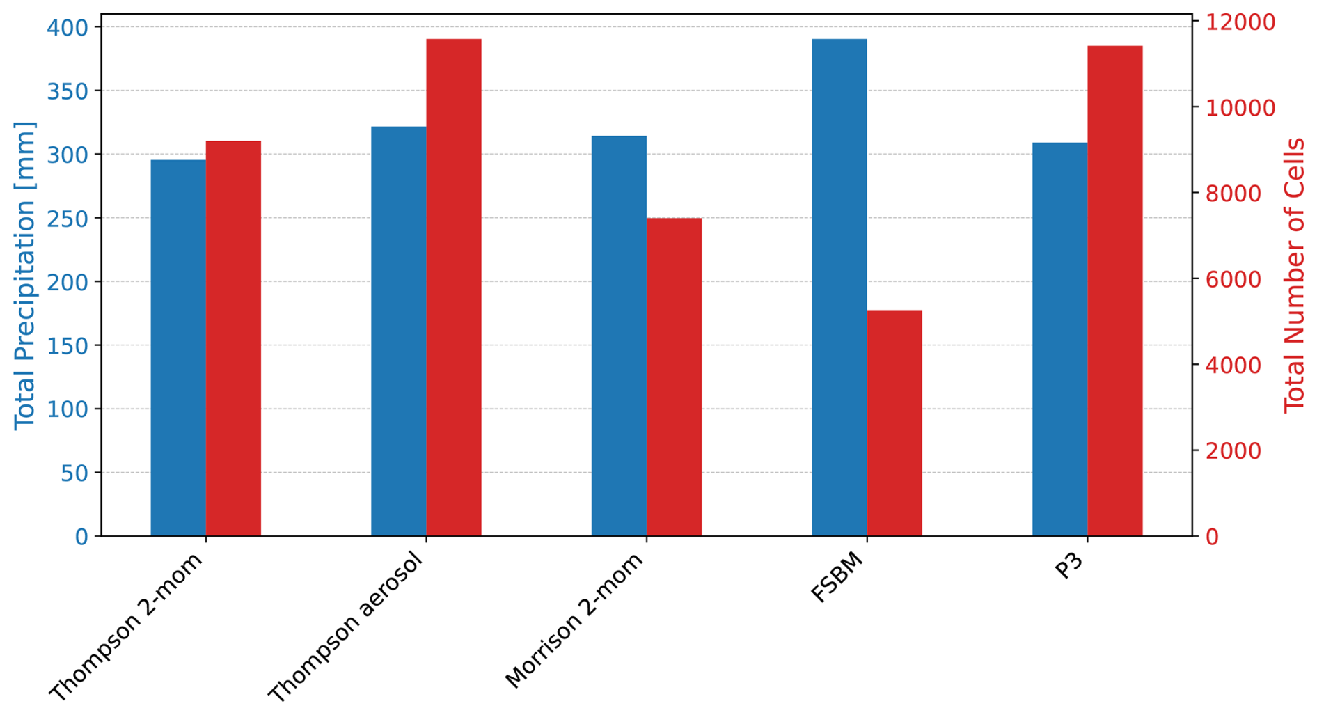
Figure 2 Total WRF simulated precipitation (blue) over all timesteps and all grid boxes as well as total number of identified convective cells (red) for each of the 5 microphysics schemes.

3.1 Vertical distribution of reflectivity signals

In order to further evaluate the spatial distribution of precipitation, we next analyze the vertical distribution of the reflectivity signals. Figure 3 shows the vertical distribution of the precipitation fraction based on reflectivity, i.e., the fraction of pixels that exceeded 5 and 35 dBZ depending on height. A stark difference can be seen between the microphysics schemes up to about 4 km for the convective (35 dBZ) threshold and over the full vertical profile for the (stratiform) 5 dBZ threshold. Most apparent is the Morrison scheme (green) which produces the highest precipitation fraction throughout the profile for the stratiform threshold. At the same time, the Morrison scheme produces the second lowest cloud fraction for the convective threshold below 3.5 km. Given that the total precipitation of the Morrison scheme is not significantly different from the other schemes, this shows that the Morrison scheme produces a much larger area of precipitation with a much lower intensity in general. Another interesting observation is the P3 scheme (purple) which closely follows the observed fraction for both thresholds at upper heights, but starts to deviate at lower heights. This is especially pronounced at the convective threshold (dashed lines) and indicates that the transition from ice to rain seems to be problematic, producing a too high convective precipitation fraction at lower heights of about twice the observed fraction. This also matches the large number of convective cells identified in the P3 scheme (Fig. 2). In the following, we focus our analysis on two height levels, 1500 and 5500 m, indicated with the dashed horizontal lines in Fig. 3. This way we cover both, an upper height where we expect to observe differences in ice growth processes, as well as a lower height where we mainly expect precipitating liquid rain drops while at both heights, there is a significant variation in the fraction between the microphysics schemes and to the observations.

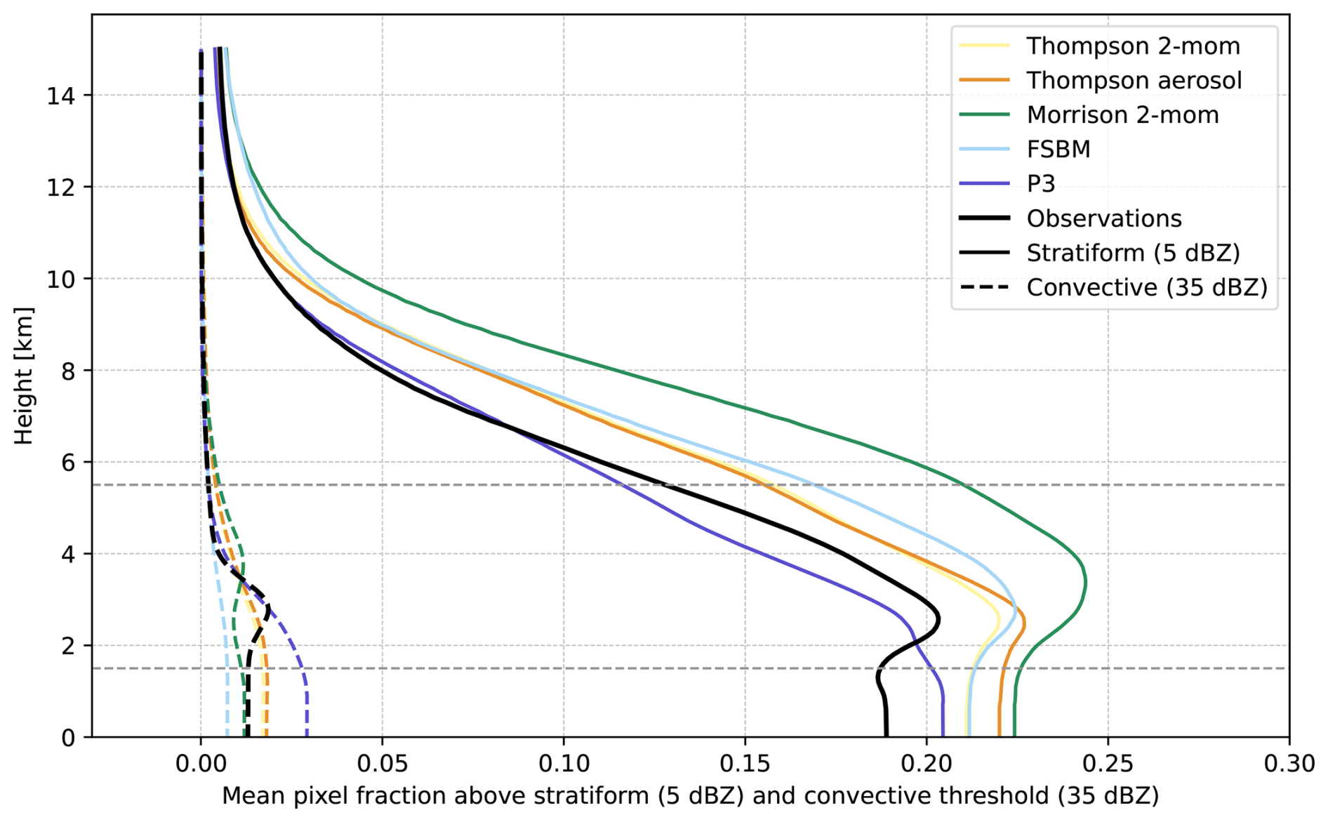
Figure 3 Vertical distribution of the mean pixel fraction larger than a 35 dBZ (dashed) and a 5 dBZ (continuos) threshold.

3.2 Distribution of convective and stratiform regions

While all schemes produced similar overall amounts of total precipitation, the distribution of precipitation into convective and stratiform regions varies significantly between the microphysics schemes. This is illustrated in Fig. 4, which shows the CAF for the 30 d data set for each of the 5 microphysics schemes and the radar observations.

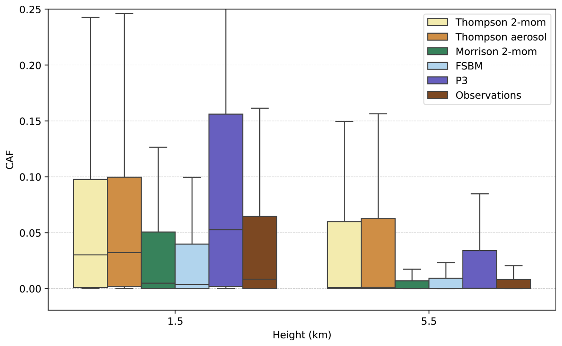
Figure 4 Convective area fraction (CAF) for the 30 d data set for each of the 5 microphysics schemes and the radar observations at two heights, 1500 and 5500 m.

The CAF is visualized using a boxplot, which shows the median (center line), the interquartile range (coloured box), and the range of the data without outliers (whiskers). Outliers are defined as data points that are more than 1.5 times the interquartile range away from the upper or lower quartile. The interquartile range is the difference between the 75th and 25th percentile of the data. Shown are two heights, 1500 and 5500 m, to illustrate the vertical distribution of the CAF.

Generally, the observations have small median CAFs of around 0.8 % at 1500 m. Morrison (0.5 %) and FSBM (0.4 %) are close and only slightly too low. The other 3 schemes have CAFs that are much too high, with the P3 scheme having the highest CAFs (5 %) followed by the Thompson schemes (3 %).

At 5500 m, the CAF is generally lower than at 1500 m, since convective cores not always reach up that high. The overall picture is similar, with a group of schemes (Thompson 2-mom, Thompson aerosol-aware and P3) producing too high CAFs and another group (Morrison and FSBM) producing close and only slightly too low CAFs. Interestingly, while P3 was highest at 1500 m, the Thompson schemes were highest at 5500 m. This is due to the fact that the Thompson schemes produce more frequently high reflectivities at 5.5 km altitude which is attributed to graupel particles (not shown). The distribution into convective and stratiform regions was also evaluated by previous studies. Shrestha et al. (2022) for example found that the CAF was underestimated by their model for 3 convective storm cases. Here, we demonstrate that the choice of microphysics schemes has a significant impact on the distribution of precipitation into convective and stratiform regions. Some schemes, especially the P3 and Thompson schemes produce CAFs that are unrealistically high compared to the observations over the 30 d dataset.

These discrepancies are due to the fact that convective reflectivities of >35 dBZ are produced too frequently in the simulations, especially below the melting layer height within rain. The simulation of these high reflectivities is driven by the underlying rain drop size distribution, which in turn is strongly influenced by microphysical processes. For example, processes such as evaporation, aggregation, or drop break-up can significantly alter the size distribution of hydrometeors and, consequently, the reflectivity. Further insight about the microphysical processes can be gained from the polarimetric radar signals, which are analyzed in the following section.

3.3 Polarimetric radar statistics

Next we will thus have a deeper look into the distributions of reflectivity (Zhh) and, especially, differential reflectivity (Z_dr) at the two height levels. The figures corresponding to the convective and stratiform regions are shown in Figs. 5 and 6, respectively. Shown are histograms of simulated and observed reflectivity (left) and differential reflectivity (right) values for the radar observations and the 5 microphysics schemes. The analysis at 5500 m altitude is shown in the upper row, while the analysis at 1500 m altitude is shown in the lower row. The values are binned into 50 bins (0.6 dBZ and 0.1 dB bins for reflectivity and differential reflectivity, respectively). Below, we provide a detailed analysis of the histograms for stratiform and convective regions separately.

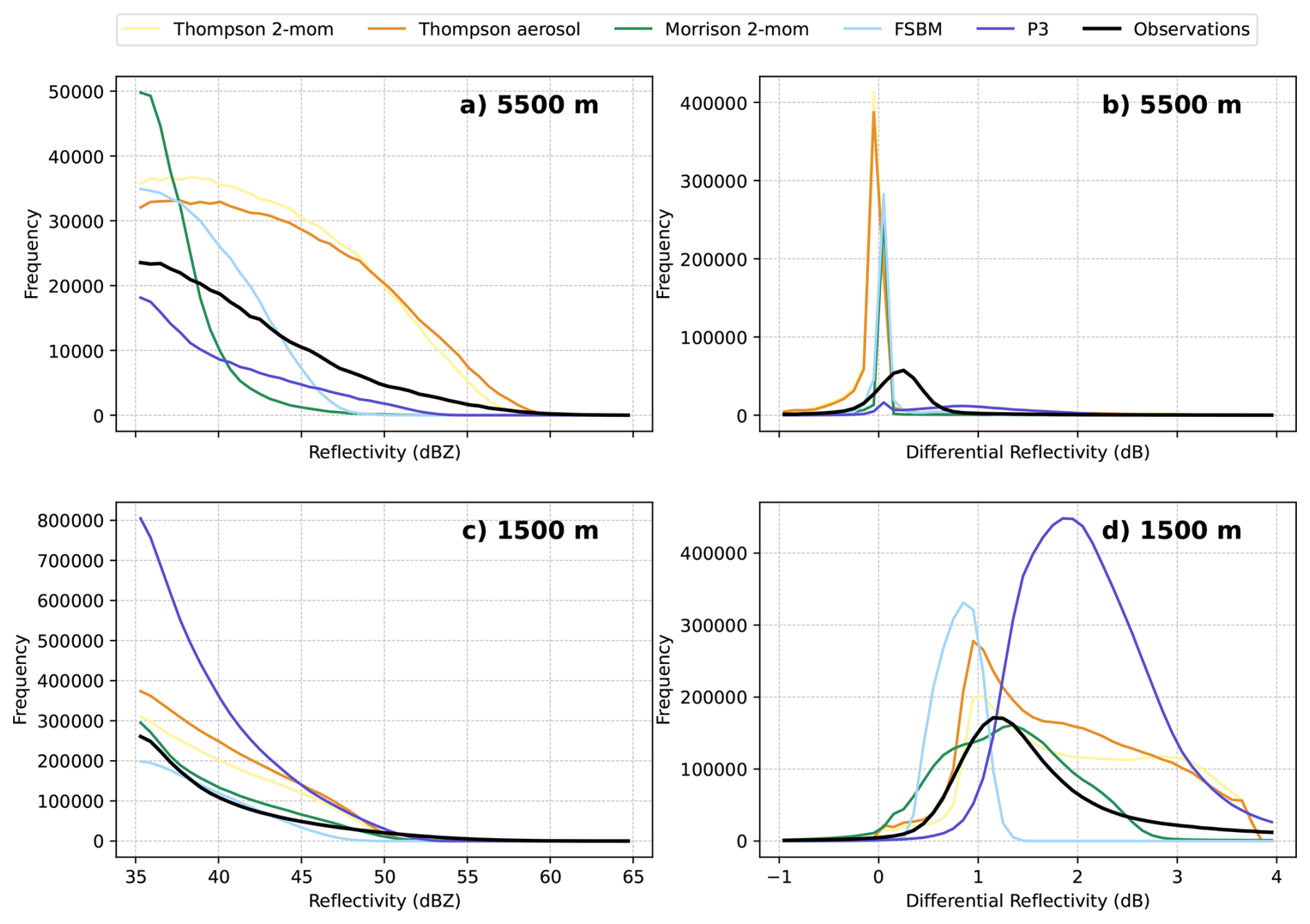
Figure 5 Histograms of simulated and observed reflectivity (a, c) and differential reflectivity (b, d) for convective precipitation at 5500 m (a, b) and 1500 m (c, d) altitude.

Figure 6 Histograms of simulated and observed reflectivity (a, c) and differential reflectivity (b, d) for stratiform precipitation at 5500 m (a, b) and 1500 m (c, d) altitude.

3.3.1 Convective region at 1500 m

The histograms for the convective region at 1500 m altitude are shown in the lower part of the picture. A comparison of the radar observations (black line) and the simulations (colored lines) reveals a significant overestimation of convective (larger than 35 dBZ) reflectivities in the reflectivity distribution (Fig. 5c)) for Thompson 2-moment, Thompson aerosol-aware, and especially the P3 scheme, The FSBM scheme on the other hand has a low bias for most of the reflectivity range, and never produced reflectivities larger than 49 dBZ.

To investigate the reason for the frequency in the reflectivity histogram, the factors that influence radar reflectivity need to be examined. In general, radar reflectivity is influenced by several factors, including the size and number of particles in the beam volume, as well as the density and phase of these particles. At an altitude of 1500 m, the predominant hydrometeor type is rain during the analyzed warm season cases. Consequently, any observed reflectivity bias may be attributable to the size and number of rain drops. It is not possible to distinguish between these potential sources of bias solely based on reflectivity. However, the differential reflectivity (Z_dr) can provide further context. Z_dr is defined as the ratio of the reflectivity received at the horizontal polarization (Zhh) to the reflectivity received at the vertical polarization (Zvv):

$$\begin{array}{}\text{(1)}& Z_{\mathrm{dr}}=\mathrm{10}{\log }_{\mathrm{10}}\left({\displaystyle \frac{Z_{\text{hh}}}{Z_{\text{vv}}}}\right)\end{array}$$

In principle, Z_dr is a measure of the aspect ratio of particles in the direction of the radar beam. For rain drops, the aspect ratio is related to their size (Ryzhkov et al., 2011). The resulting Z_dr depends on the viewing angle of the radar. From below, rain drops appear spherical to the radar, resulting in a Z_dr value of 0 dB. At low elevation angles, when the radar looks through the side of the rain particles, rain drops appear more oblate, resulting in Z_dr values larger than 0 dB. The magnitude of Z_dr is then related to the size of the rain drops, with larger rain drops producing larger Z_dr values. Importantly, Z_dr is independent of the number of particles in the beam volume. Both, Zhh and Zvv, are proportional to the number of particles in the beam volume, so any change in the number of particles cancels out in the ratio. Consequently, at low elevation angles, Z_dr can be used as a measure of rain drop size.

The Z_dr histograms for the convective region at 1500 m altitude are shown in Fig. 5d). The observations exhibit a Z_dr distribution that has a peak at about 1.2 dB and is skewed to the right, with a tail extending to higher values. In general, the simulations exhibit similar distributions, but with a notable bias towards higher or lower values, depending on the scheme. The FSBM scheme has a strong low bias, generating Z_dr values below 1 dB to frequently, while Z_dr values above 1.5 dB are not simulated at all. The Thompson schemes and particularly the P3 scheme demonstrate a high bias in Z_dr, simulating high Z_dr values of more than 2 dB too frequently. This correlates well with the reflectivity distribution in Fig. 5c). We conclude that the high area fraction of convective precipitation in the P3 and Thompson schemes is due to rain drop sizes that are too large, while the FSBM scheme misses large rain drops and produces too many small rain drops. The Morrison scheme also exhibits low bias in Z_dr, though less pronounced. The Morrison scheme exhibits a tendency to simulate Z_dr values lower than 1 dB with a higher frequency than observed, yet failed to generate Z_dr values greater than 3 dB, despite the existence of such observations. However, this does not translate into a low reflectivity bias. This suggests that large drops were missing in the Morrison scheme relative to the observations, but a large number of droplets compensates for this providing sufficient reflectivity still. Sun et al. (2023) noted a similar lack of large rain drops in the convective part of a squall line in the Morrison scheme. In this study, we demonstrate that this phenomenon is consistent across multiple days and different convective events. However, Sun et al. (2023) reported a low bias of reflectivity in the convective region for the Morrison scheme in their squall line case, which we cannot find based on our simulations. Planche et al. (2019) on the other hand find a high reflectivity bias in the convective part of their squall line case simulation with the Morrison scheme, in line with our findings. This underscores the high variability in the performance of microphysics schemes across different convective events and highlights the strength of a statistical approach.

Relating these findings to the biases in CAF (Fig. 4), we see a strong correlation between the high fraction of convective precipitation in the P3 and Thompson schemes and the high bias in the reflectivity and Z_dr histograms. Thus, we conclude that the P3 and Thompson schemes produce a convective precipitation area that is too large, which is a result of the frequent occurence of large rain drops that produce high reflectivities and Z_dr values. The FSBM scheme, on the other hand, produces a low fraction of convective precipitation due to the low frequency of large rain drops. This could mean that rain within the P3 and Thompson simulations is generally more intense, but also more localized, while the FSBM scheme produces a more widespread and less intense rain.

3.3.2 Convective region at 5500 m

The reflectivity and differential reflectivity histograms for the convective region at an altitude of 5500 m are shown in Fig. 5a and b, respectively. These heights provide some context to the preceding analysis conducted at 1500 m altitude, because at mid-latitudes, rain typically originates from melting ice phase particles present at this altitude. Figure 5a reveals an overall overestimation of convective (larger 35 dBZ) reflectivities by most schemes. While FSBM and Morrison somewhat compensate for this by a lack of largest values, both Thompson do not. Only P3 shows a deficit of these convective reflectivites in general. The Thompson schemes demonstrate analogous biases at this altitude as observed at 1500 m altitude, e.g., the Thompson schemes exhibit a consistent high bias, generating convective reflectivities too frequently over the entire reflectivity range. This suggests that the issues in the convective core at 1500 m altitude for these schemes stem from the ice phase. For example, in the Thompson schemes, high reflectivities at 1500 m altitude due to rain drop sizes that are too large might be a result of melting ice phase particles that are already too large at 5500 m altitude. Planche et al. (2019) for example show that the rain drop size distribution is very sensitive to the melting process within the Thompson scheme, although their focus was on the melting of snow.

The Morrison scheme exhibits a notable low bias at 5500 m altitude, resulting in low reflectivities of 39 dBZ and below being produced too frequently and reflectivities above 39 dBZ being produced too infrequently. This does not translate into a low reflectivity bias at 1500 m altitude. However, it might explain the low bias in Z_dr at 1500 m altitude, as the Morrison scheme produces a low fraction of large rain drops at 1500 m altitude, based on the Z_dr histogram (Fig. 5d).

To provide further context, the Z_dr histograms for the convective region at 5500 m altitude are shown in Fig. 5b. At this altitude, the radar forward operator assumptions regarding the ice shape significantly influence the simulated Z_dr. The P3 scheme diverges from the other schemes in the ice phase by employing a single ice class, whereas the other schemes utilize multiple ice classes. Consequently, the forward operator assumptions differ between the P3 scheme and the other schemes. Further uncertainties arise from the fact that the radar forward operator must assume ice particle shapes as well as particle orientations, which are not simulated directly by the WRF model. Due to the significant impact of these radar forward operator assumptions on the differential reflectivity in the ice phase we refrain from further analysis of the Z_dr histograms at 5500 m altitude.

Unfortunately, this means we cannot provide a clear explanation for the bias in reflectivity at 5500 m altitude. However, with the radar forward operator applied in this study (CR-SIM), it is possible to distinguish between the contributions of different hydrometeor classes to the radar signals. Large reflectivities of more than 30 dBZ at 5500 m altitude are typically associated with graupel particles. We find that the P3 scheme produce graupel-induced reflectivities of only up to 30 dBZ, Morrison and FSBM schemes of up to 40 dBZ, while the Thompson schemes frequently yield graupel reflectivities exceeding 50 dBZ (not shown). We conclude that the bias in reflectivity in the convective core is attributable to graupel particles, where graupel is underrepresented in the P3, Morrison and FSBM scheme, but overrepresented in the Thompson schemes. However, we cannot distinguish between the effects of number concentration, density assumption or graupel size on the reflectivity bias. Graupel was also identified as a potential important source of bias in other studies. Sun et al. (2023) for example proposed an underprediction of ice-phase processes associated with graupel and hail, such as riming, as the likely cause for the aforementioned lack of large rain drops in the Morrison scheme within the context of a squall line case. A different study by Shrestha et al. (2022) revealed that melting of graupel was the dominant rain mechanism in COSMO simulations of 3 convective storms, whereas the observations indicated a different mechanism.

3.3.3 Stratiform region at 1500 m

Figure 6 illustrates the histograms for the stratiform region. At an altitude of 1500 m, the majority of the schemes exhibit a low bias in reflectivity (Fig. 6c). This phenomenon is particularly evident in the Morrison and FSBM schemes, who simulate reflectivity values below 25 dBZ too frequently and reflectivity values above 25 dBZ too infrequently. The Thompson schemes, produce a peak at the correct reflectivity; however, all schemes produce low reflectivities much too often. This was of course also evident in Fig. 3. Only the P3 scheme distribution is very similar to the observed distribution, however, the frequency over the entire range is slightly too high.

Once more, Z_dr provides further context (Fig. 6d). In this case, all schemes except for the P3 scheme demonstrate a pronounced low bias in Z_dr, where Z_dr below 0.3–0.5 dB is simulated too frequently and higher Z_dr is simulated too rarely. This suggests that in the stratiform region at 1500 m, all schemes except the P3 scheme simulate large rain drops less often than observed. This pattern is consistent with the convective region at 1500 m altitude for the Morrison and FSBM schemes, where a low bias in Z_dr is also observed and is attributed again to a low frequency of large rain drops. While our findings in the convective regions were in line with the findings of Sun et al. (2023), the results in the stratiform region are not. Sun et al. (2023) reported an excessive proportion of large drops for the Morrison scheme for the stratiform regions of their squall line case, whereas we find that over a 30 d dataset, the Morrison scheme exhibits a low bias in Z_dr in the stratiform regions. A possible explanation for this discrepancy could be that the large drops that Sun et al. (2023) find in the stratiform region of their squall line is a case specific phenomenon, which is not a general bias of the Morrison scheme.

The Morrison and FSBM distributions exhibited similar characteristics both in the stratiform and convective regions at 1500 m altitude, e.g., largest Z_dr values were simulated too rarely. In contrast, the Thompson schemes exhibit a completely different behavior in the stratiform region compared to the convective region at 1500 m altitude. There is a clear overestimation of large Z_dr values in the convective region, while in the stratiform region, the Thompson schemes exhibit a low bias in Z_dr. This could indicate that large particles might fall out within the convective region too efficiently, resulting in a low amount of large particles transported via the ice phase into the stratiform region.

Previous studies reported contradictory results regarding rain size biases in the Thompson schemes. Wu et al. (2021) found that their simulation of a typhoon event with the Thompson 2-mom scheme produced a frequency of large rain drops lower than observed. Putnam et al. (2016) on the other hand found that the Thompson 2-mom scheme produced reflectivity values that are too high and attributed this among other things to a high frequency of large rain drops. Our findings suggest that the Thompson schemes produce a relatively high frequency of large rain drops in the convective region, but a relatively low frequency of large rain drops in the stratiform region, which might explain the contradictory findings in previous literature. The P3 scheme is the only scheme that exhibits a Z_dr distribution that closely resembles the observations, with only a marginal shift towards higher Z_dr values, suggesting that the frequency of large rain drops is more prevalent in the P3 scheme than what is observed. This is consistent with the findings in the convective region at 1500 m altitude, where the P3 scheme also produced a high frequency of large rain drops. However, this bias is much less pronounced in the stratiform region than in the convective region at 1500 m altitude.

3.3.4 Stratiform region at 5500 m

The reflectivity histograms for the stratiform region at an altitude of 5500 m (Fig. 6a) reveal that all schemes produce too large areas of the shown reflectivity levels, but that they do not exhibit a substantial bias. In general, stratiform reflectivities are simulated more frequently than what was observed over most of the reflectivity range for all schemes except the P3 scheme. This is most pronounced for weaker reflectivities below 25 dBZ for all schemes except for the Morrison scheme. The Morrison scheme exhibits a notable deviation of approximately 5 dB towards higher reflectivity values. This finding has been reported in other studies and appears to be a persistent issue with the Morrison scheme. For instance, Planche et al. (2019) reported overestimations of simulated reflectivity of more than 10 dB between 5 and 10 km in their squall line case, attributing this to either snow density assumptions or an excessive number of large snow particles. Sun et al. (2023) also found that the Morrison scheme produced reflectivity values that were too high in the stratiform region below the −20 °C level for their squall line case and attribute this to high assumed graupel densities or too large graupel fractions. In our simulations, we find that reflectivities larger than 25 dBZ at 5.5 km altitude are primarily associated with snow particles in the Morrison scheme simulations (not shown).

Interestingly, the correlation of biases between 1500 and 5500 m altitude is significantly lower for the stratiform region than for the convective region. The Morrison scheme even has a pronounced high bias at 5500 m altitude, contrasting with the low bias at 1500 m. This suggests that the origin of biases at 1500 m may not be exclusively attributed to the ice phase for the Morrison scheme within the stratiform region. The disparities in the drop size distributions within the stratiform region may also be attributable to the representation of warm rain processes, such as collisional breakup, collision-coalescence or evaporation. For instance, Planche et al. (2019) reported an unrealistic strong vertical change of drop size diameter and number concentration in the stratiform region of the Morrison simulation of a squall line, due to the representation of warm rain processes in the Morrison scheme. Sun et al. (2023) further reported an overly strong collision-coalescence process in the Morrison scheme for their squall line case in the stratiform region. The Z_dr histograms for the stratiform region at 5500 m altitude are displayed in Fig. 6b. It is evident that no simulation was capable of reproducing the observed Z_dr distribution, as all of them exhibited a pronounced peak at approximately 0 dB and almost no values above 0.1 dB. In contrast, the observed distribution is much broader, encompassing values up to 1 dB more frequently. The discrepancy in the Z_dr histograms at 5500 m altitude can be attributed to the inherent assumptions of the radar forward operator concerning the particle shapes. Given the similarity in bias observed among all schemes, we refrain from further interpretation of the Z_dr histograms at 5500 m altitude.

3.4 Simulated rain drop size distributions

In the previous section, issues in the simulated reflectivity and differential reflectivity at 1500 m altitude were mainly attributed to the size of rain drops. While we do not have real observations of the size distribution of rain drops, we can analyze the simulated size distributions of rain drops in the model output. This helps to understand if the differences in the simulated reflectivity and differential reflectivity are indeed due to differences in the size distribution of rain drops. Figure 7 shows the total number of simulated rain drop sizes over all 30 d at 1500 m altitude for the 5 microphysics schemes for the convective and stratiform regions. The size distributions of the bulk schemes are binned into 17 bins that correspond to the bins used in the FSBM scheme. In general, the distributions within the convective regions and stratiform regions look similar. The area covered by stratiform precipitation is generally larger than the area covered by convective precipitation (see Fig. 3). Therefore, the total number of drops in the stratiform region is also generally larger than in the convective region. However, the difference in the number of drops between the two regions is not constant across all drop sizes. For small drops, the number of drops in the stratiform region is significantly larger than in the convective region, by up to 1–2 orders of magnitude. In contrast, the number of large drops of about 4 mm is similar in both, the convective and stratiform regions. This demonstrates that within the convective region, the drop size distribution is shifted towards larger drops, while in the stratiform region, the distribution is shifted towards smaller drops.

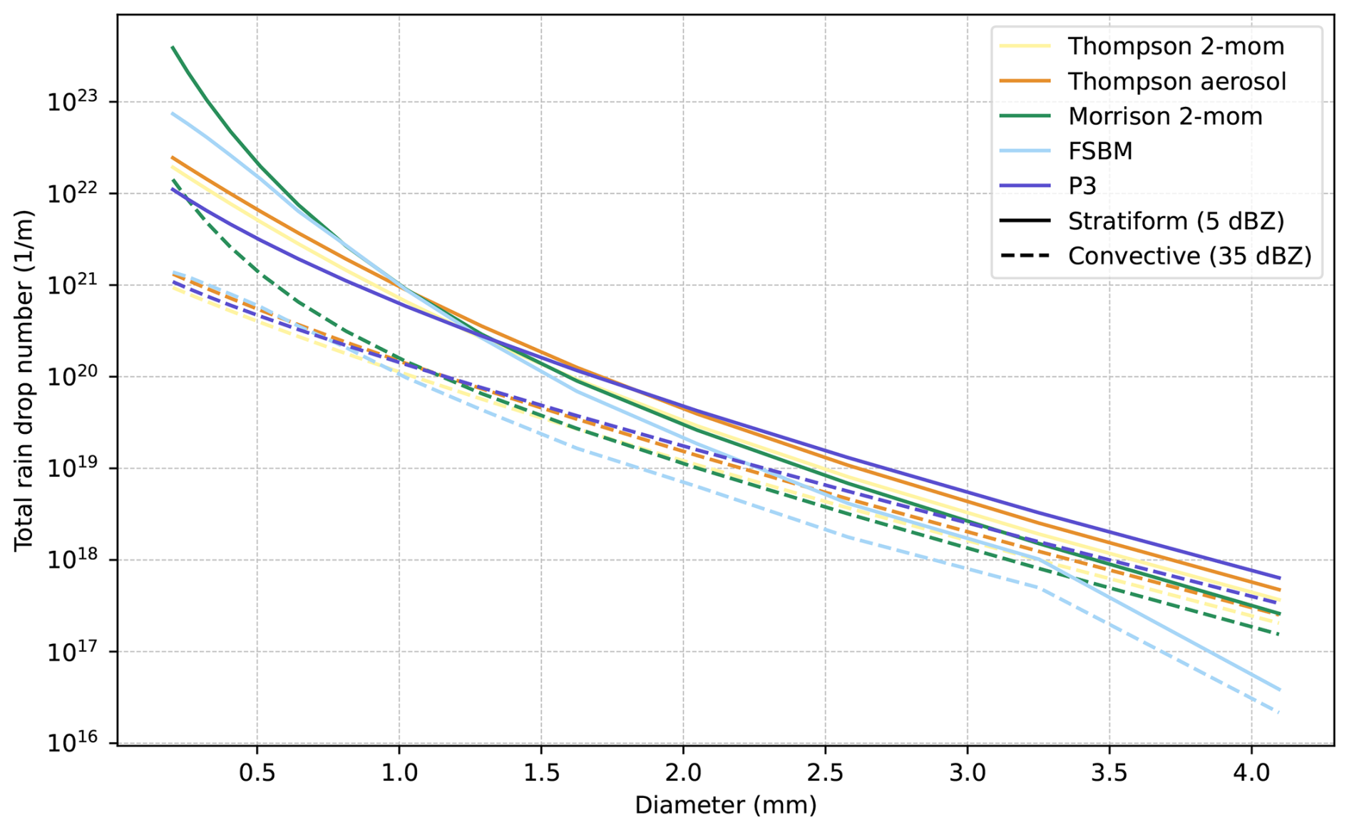
Figure 7 Total simulated number of rain drops for the convective (dashed lines) and stratiform (continous lines) regions at 1500 m altitude for the 5 microphysics schemes.

The microphysics schemes also impact the size distribution of rain drops. The Morrison and FSBM schemes produce a higher number of small drops, and the lowest number of large drops. The P3 scheme is the exact opposite, producing the highest number of large drops and the lowest number of small drops, while the Thompson schemes are in between. This is true for both regions, convective as well as stratiform, but the differences are more pronounced in the stratiform region, especially for small drops. This is consistent with the interpretations in the previous sections. The schemes that produced the highest Z_dr values (Thompson and P3) also produced the highest number of large drops in the size distribution, while the schemes that produced the lowest Z_dr values (Morrison and FSBM) also produced the lowest number of large drops in the size distribution. This provides confidence in our conclusions regarding the rain drop size distributions based on the simulated differential radar reflectivity Z_dr.

4 Summary and conclusions

The representation of cloud microphysics in numerical weather prediction models are subject to large uncertainties (Morrison et al., 2020; Fan et al., 2017). Particularly challenging is the prediction of convective precipitation events, due to their small scale and rapid error growth of initial uncertainties (Selz and Craig, 2015; Hohenegger and Schär, 2007). In this study, the performance of five different microphysics schemes in the simulation of convective precipitation events is analyzed statistically over a 30 d dataset in 2019 and 2020. The simulations are conducted using the Weather Research and Forecasting (WRF) model, employing a regional limited area model setup over Munich with a horizontal grid spacing of 400 m. 5 different microphysics schemes are utilized: the Thompson 2-moment scheme (Thompson 2-mom; Thompson et al., 2008), the Morrison 2-moment scheme (Morrison 2-mom; Morrison et al., 2009), the Thompson aerosol-aware scheme (Thompson aeresol-aware; Thompson and Eidhammer, 2014), the fast spectral bin microphysics scheme (FSBM; Shpund et al., 2019), and the Predicted Particle Properties scheme (P3; Morrison and Milbrandt, 2015). The simulations are then compared to polarimetric radar observations from the German Meteorological Service (DWD) radar network, i.e., reflectivity (Z) and differential reflectivity (Z_dr). The convective and stratiform regions are separated using an automatic cell-tracking algorithm, tobac (Sokolowsky et al., 2024). The convective area fraction (CAF) is a metric employed to assess the distribution of precipitation into convective and stratiform regions. While the total precipitation amounts are comparable for all schemes, the distribution into convective and stratiform regions varies significantly. The Thompson schemes and P3 exhibit higher CAFs compared to the observed values, while the Morrison schemes and FSBM demonstrate close, though slightly lower CAFs. The discrepancies are mainly a result of differences in the simulated convective area, rather than the stratiform area. This underscores the pivotal role that the choice of microphysics schemes plays in determining the distribution of precipitation into convective and stratiform regions.

To investigate microphysical reasons for the differences in precipitation distributions, an analysis of simulated and observed reflectivity and differential reflectivity histograms is conducted for the convective and stratiform regions at two altitudes, 1500 and 5500 m. Polarimetric radar signals are influenced by the size and number of the particles in the beam volume, as well as the density and phase of the particles. This allows for an interpretation of the biases in reflectivity and differential reflectivity in terms of the microphysical properties of the simulated particles. The following conclusions are derived from the analysis of the radar signal histograms:

Convective Core

1. At an altitude of 1500 m, FSBM and Morrison simulations frequently lack large rain drops. For the FSBM scheme, this results in a low bias in reflectivity. For the Morrison scheme this is not the case as it is compensated by a high number of small drops.

2. The Thompson schemes and P3 produce an excessive number of high Z_dr values, indicating that large rain drops are too frequent in these schemes. This is consistent with the simulated rain drop size distributions.

3. The Thompson schemes exhibit comparable biases in reflectivity at 1500 and 5500 m altitude, indicating that these biases originate in the ice phase.

Sun et al. (2023) also reported a lack of large rain drops in the convective part of a squall line in the Morrison scheme, a finding consistent with our results. Here, we demonstrate that this is persistent across multiple days and different convective events. Contradictory results have been reported in other studies concerning the reflectivity biases of the Morrison scheme. Sun et al. (2023), for instance, reported a low bias within the convective region for their squall line case, while Planche et al. (2019) found a high bias in the convective part for their squall line case. This demonstrates the high variability of the performance of microphysics schemes for different convective events and the strength of a statistical approach.

Stratiform region

1. Only the P3 scheme produces a sufficient number of large rain drops, while all other schemes produce too few large rain drops, resulting in a low bias in Z_dr and reflectivity.

2. At an altitude of 5500 m, the Morrison scheme exhibits a significant high bias in reflectivity.

3. There is no significant correlation between distributions at 1500 and 5500 m altitude, indicating that the origin of the bias is not necessarily in the ice phase.

Other studies also reported that the Morrison scheme yielded reflectivity values that were excessively high in the stratiform region at upper heights. Planche et al. (2019), for instance, reported overestimations of Morrison's simulated reflectivity of more than 10 dB between 5 and 10 km altitude for their squall line case. They attributed this to either snow density assumptions or too many large snow particles. Sun et al. (2023) also found that the Morrison scheme produced reflectivity values that were too high in the stratiform region below the −20 °C level for their squall line case and attributed this to graupel densities or too large graupel fractions.

In general, the Morrison and FSBM schemes exhibit similar biases in Z_dr in the stratiform and convective regions at 1500 m altitude, i.e., low Z_dr values are simulated too frequently in both regions. The Thompson schemes on the other hand have a bias in Z_dr at 1500 m altitude in the convective region, but a low bias in Z_dr at 1500 m altitude in the stratiform region. This could indicate that large particles might sediment too efficiently within the convective region, resulting in a low amount of large particles transported via the ice phase into the stratiform region. Previous studies reported contradictory results regarding rain size biases in the Thompson schemes. For example, Wu et al. (2021) reported a frequency of large drops lower than observed, while Putnam et al. (2016) found that the Thompson 2-mom scheme produced reflectivity values that are too high and attributed this to a high frequency of large rain drops. Our findings suggest that the Thompson schemes do not generally exhibit a size bias in rain drops, but that the size bias is dependent on the region. This might explain the contradictory findings in previous literature.

Relating the analysis based on the polarimetric radar signals to the precipitation distribution based on the CAF, we find a strong correlation between the high fraction of convective precipitation in the P3 and Thompson schemes and the high bias in reflectivity and Z_dr histograms. We conclude that the high CAF in the P3 and Thompson schemes is due to the high frequency of large rain drops that produce high reflectivities and Z_dr values. This translates into an unrealistic high fraction of convective precipitation in the P3 and Thompson schemes. With the same argument, we conclude that the missing large drops in the FSBM and Morrison scheme translate into a low CAF, although this is not as pronounced as in the P3 and Thompson schemes.

In general, the majority of the observed biases in reflectivity and Z_dr can be attributed to issues in the simulation of particle size distributions. Analysis of the underlying simulated rain drop size distributions (DSDs) supports these interpretations of the Z_dr signals. This is of particular significance, because the representation of particle size distributions is crucial for the accurate simulation of precipitation.

Our study shows that the choice of microphysics schemes has a significant impact on the rain drop size distributions, which in turn affects the distribution of precipitation into intense localized convective and more widespread, weaker stratiform regions. We demonstrate how polarimetric radar observations can be used to identify issues in the underlying particle size distributions of the microphysics schemes. In contrast to previous studies that evaluate microphysics schemes typically based on case studies, our evaluation encompasses a dataset over 30 d of convective precipitation events. This provides a more robust estimate of the performance of microphysics schemes. In light of the increasing accessibility of operational polarimetric radar observations, our study has the potential to provide a framework for the rigorous statistical evaluation of weather models using polarimetric radar measurements, extending this capability to other regions and weather scenarios. However, within the scope of this study, we focused only on one polarimetric radar variable, Z_dr. Future research could expand the analysis to include additional polarimetric radar variables, such as specific differential phase (K_dp) or correlation coefficient (RHOhv), which could provide further insights into the microphysical properties of the different microphysics schemes. K_dp, for instance, can provide information on number concentration of rain drops in the radar beam volume, while RHOhv can provide information on the presence of mixed-phase precipitation (Bringi and Chandrasekar, 2001, Chapter 7). K_dp and RHOhv in combination with Z_dr and Z could also be used for hydrometeor classification (e.g.,  Dolan et al., 2013).

While polarimetric radar measurements can provide valuable insights into the microphysical properties of hydrometeors, exact conclusions regarding the DSDs could be derived through the use of disdrometer measurements or retrievals, such as Dual-Wavelength retrievals. Li et al. (2023), for instance, evaluated a simulation of an extreme rainfall event over China using disdrometer measurements and underscored the importance of drop size distributions when analyzing extreme rainfall events.

Furthermore, the radar forward operator assumptions on the particle shapes exert a substantial influence on the simulated Z_dr for ice phase particles. This hinders the interpretation of the Z_dr histograms at 5500 m altitude in this study. The use of a more sophisticated radar forward operator that does not rely on the T-matrix method could provide more insights into the microphysical properties of the different microphysics schemes. Alternatively, the utilization of schemes that provide more detailed information on the particle shapes and orientations could mitigate the uncertainties in the radar forward operator assumptions.

Finally, this study did not consider cell lifetime stage. However, with cell tracking tools such as tobac, it is possible to obtain further insights into the microphysical properties of the different microphysics schemes during various stages of a convective cell's lifetime. This could be a topic for future research.