Bias correcting regional scale Earth system model projections: novel approach using empirical mode decomposition

Bias correction is a crucial step in using Earth system model outputs for assessments, as it adjusts systematic errors by comparing the model to observations. However, standard methods – ranging from mean-based linear scaling to distribution-based quantile mapping typically treat bias correction as a single-scale process, overlooking the fact that biases can manifest differently across daily, seasonal, and annual timescales. In this study, we propose a novel, timescale-aware bias-correction approach built on Empirical Mode Decomposition. By decomposing the meteorological signal into multiple oscillatory components and aggregating them to represent distinct timescales, we apply targeted corrections to each component, thereby preserving both short- and long-term structure in the data. Experimental illustrations show that the timescale-aware EMDBC framework matches the performance of conventional quantile-delta mapping (QDM) at the native daily scale and achieves progressively larger bias reductions at bi-weekly, seasonal, and annual scales. As a result, the proposed approach offers a more robust path to accurate and reliable Earth system projections, strengthening their utility for resilience and adaptation planning.

1 Introduction

Accurate projections of future weather dynamics at regional and local scales are crucial not only for understanding extremes but also for guiding decision-making in sectors such as water resource management, agriculture, renewable energy, and public health. Over the decades, the horizontal spatial resolution of large-scale models, including global climate models (GCMs), has significantly improved, with grid cells for CMIP6 (Coupled Model Intercomparison Project Phase 6) models typically ranging from 50 to 100 km (Masson-Delmotte et al., 2021; Roberts et al., 2019). However, most resilience and preparedness efforts demand meteorological inputs at spatial and temporal scales much finer than the resolution of the latest GCMs (Kotamarthi et al., 2021). Consequently, current state-of-the-art GCMs still fall short in providing the fine-scale resolution required for detailed assessments in many sectors. Common approaches to addressing the scale gap between information from GCMs and the needs for actionable regional and local-scale information include statistical (Fan et al., 2013; Pierce et al., 2014) and dynamical downscaling (Prein et al., 2015; Wang and Kotamarthi, 2014, 2015; Akinsanola et al., 2024) approaches. Unlike statistical downscaling which relies on drawing empirical relationships between large-scale Earth system models and local observations to infer fine-scale meteorological information, dynamical downscaling can simulate a range of physical processes and their interactions within the Earth system, producing a comprehensive set of dynamically consistent high-resolution atmospheric variables. The standard practice of dynamical downscaling involves the continuous operation of a regional climate model (RCM), using outputs from GCMs as initial and lateral boundary conditions. Various region-level modeling and assessment initiatives have adopted this approach, including the North American Regional Climate Change Assessment Program (Mearns et al., 2012), the North American component of the Coordinated Regional Downscaling Experiment (NA-CORDEX) (Mearns et al., 2017), targeted evaluations for Tasmania (Corney et al., 2013), the central United States (Bukovsky and Karoly, 2011), the European Coordinated Regional Downscaling Experiment (EURO-CORDEX) ensemble over Europe (Jacob et al., 2014), and the Coordinated Regional Downscaling Experiment over Africa (CORDEX-Africa) initiative (Nikulin et al., 2012), demonstrating the enhanced capability to capture fine-scale features and provide more realistic, detailed projections at regional and local scales. Despite these improvements, RCMs continue to face challenges with biases arising from both their forcing data and inherent systematic errors, such as those related to model resolution (Christensen et al., 2008), simplified physical parameterizations (Misra, 2007; Bukovsky and Karoly, 2011; Jacob et al., 2014), and incomplete understanding of the Earth system (Christensen et al., 2008), all of which degrade the downscaled simulations.

To address these biases and improve the reliability of future projections, various bias correction (BC) methods have been developed and employed in many studies. One of the simplest approaches is the mean-based linear scaling BC method (Tumsa, 2021). It involves calculating the difference between the mean of the historical output of the model and the mean of the observed data. The difference is then added to the future projections, scaling the model data based on the mean difference between model and observations calculated in the historical record. However, this method assumes that the relationship between model and observed data is linear with time and over the entire distribution of the variable. However, this may not capture more complex biases, especially for extreme events or in cases where the distribution of the data differs significantly between the model and observations or between the present and future projections. Furthermore, it only adjusts the mean and does not address other statistical moments, such as variability or skewness, potentially limiting its effectiveness in accurately representing the full range of weather conditions. Building on the mean-variance trend correction approach introduced by Xu and Yang (2015), Xu et al. (2021) proposed a novel bias correction method that adjusts both the linear mean and nonlinear variance trends in model-simulated series. The most commonly used bias-correction method, quantile mapping (QM), addresses several limitations of the mean-based linear scaling BC method by providing a more flexible and detailed approach to correcting biases in Earth system model outputs. The QM method preserves the full distribution of the data by mapping the entire cumulative distribution function (CDF) of the model data to that of the observed data. This ensures that the corrected model data reflect not just the mean, but also the variability, extremes, and other statistical characteristics of the observed data. In the QM method, a transfer function is created by matching model‐simulated and observed quantiles at their common temporal resolution (daily in this study) during a reference period; this function is then applied to future model simulations. The method is typically evaluated by comparing bias-corrected values with observations to assess performance. Previous studies have shown that QM effectively removes biases, improving model accuracy for both mean values (Wood, 2002; Wood et al., 2004; Boé et al., 2007; Piani et al., 2009) and extreme events (Piani et al., 2010; Ashfaq et al., 2010; Teutschbein and Seibert, 2012; Gudmundsson, 2012). However, since QM assumes that the CDF for a variable remains unchanged in future periods, it may distort signals and corrupt future trends, as the CDF is expected to shift in future projections. An alternative bias-correction method, Quantile Delta Mapping (QDM) (Cannon et al., 2015; Tong et al., 2021), improves upon QM by not only matching the CDF of modeled and observed data, but also accounting for shifts in these distributions over time, especially under future scenarios. Yet, it still assumes stationarity in the quantile-based difference (delta) over time and typically does not consider the timescale-dependent nature of biases. A more detailed discussion of QM and QDM is provided in Sect. 2.2. Several ML-based bias-correction schemes have been proposed as well (e.g., Sarhadi et al., 2016; Miftahurrohmah et al., 2024; Das et al., 2022; Feng et al., 2024); however, comprehensive intercomparisons such as Dhawan et al. (2024) show that their daily-scale performance is broadly comparable to that of quantile-based approaches like QDM and that none addresses biases occurring across multiple distinct timescales.

Indeed, biases can manifest differently at daily, monthly, seasonal, and annual scales (Haerter et al., 2011), and a correction that is effective at one timescale may fail at another and introduce inconsistencies. Although quantile-based methods like QDM can capture shifts in the overall distribution, they typically treat the data as a single timescale, thereby limiting their ability to capture biases that manifest differently across daily, monthly, seasonal, or annual timescales. Furthermore, even when acknowledging that biases may vary with timescale, isolating and representing these distinct fluctuations in the raw data is a non-trivial task. To address these gaps, we propose an Empirical Mode Decomposition-based Bias Correction (EMDBC) framework, leveraging the adaptive nature of Empirical Mode Decomposition (EMD) (Huang et al., 1998) and its ensemble variant Ensemble-EMD (EEMD) (Wu and Huang, 2009) to isolate distinct oscillatory modes at multiple timescales. By bias-correcting each extracted component (e.g., via QDM or quantile regressions) and then recombining them, EMDBC maintains key physical relationships and effectively addresses both high-frequency and low-frequency biases that conventional methods may overlook.

The remainder of this manuscript is organized as follows. Section 2 describes the experimental setup, reviews conventional BC approaches, and introduces the proposed EMDBC framework. Section 3 evaluates EMDBC's performance in a validation context and applies it to bias-correct large-scale regional Earth system model outputs. Finally, Sect. 4 summarizes the findings, discusses limitations, and suggests avenues for future research.

2 Methods

2.1 Data

This study utilizes both observed and modeled temperature datasets over the continental United States to bias-correct regional-scale Earth system model projections. The datasets are described as follows:

• WRF-CCSM (Wang and Kotamarthi, 2015): building off of previous studies (Wang and Kotamarthi, 2014, 2015), this study uses modeled 3-hourly temperature data at a 12 km spatial resolution for three time periods–historical (1995–2004), mid-century (2045–2054), and late-century (2085–2094). These projections, called WRF-CCSM, are generated by dynamically downscaling the Community Climate System Model version 4 (CCSM4) using the Weather Research and Forecasting (WRF) model version 3.3.1 (Skamarock et al., 2008). For future periods (mid- and late-century), we use the Representative Concentration Pathway 8.5 (RCP8.5) scenario, which corresponds to a high greenhouse gas concentration trajectory, reaching approximately 8.5 W m⁻² of radiative forcing by 2100 (Riahi et al., 2011). The model uses the Grell–Devenyi convective parametrization (Grell and Dévényi, 2002), the Yonsei University planetary boundary layer scheme (Noh et al., 2003), the Noah land surface model (Chen and Dudhia, 2001), the longwave and shortwave radiative schemes of the Rapid Radiation Transfer Model for GCM (Iacono et al., 2008), and the Morrison microphysics scheme (Morrison et al., 2009). Spectral nudging (Miguez-Macho et al., 2004) is applied at 6-hour intervals to large-scale features, including air temperature, geopotential height, and wind, for levels above 850 hPa and wavelengths around 1200 km, using a nudging coefficient of $\mathrm{3}\times {\mathrm{10}}^{-\mathrm{5}}$ s⁻¹. Additionally, a 1-year spin-up period is implemented to allow the model to reach equilibrium before each of the three simulations. Details on the model design and configurations are provided in Wang and Kotamarthi (2014) and Wang and Kotamarthi (2015).

• Livneh (Livneh et al., 2013): observed daily temperature data at a 1/16° spatial resolution for the historical period (1995–2004). Livneh temperature data is generated from daily temperature observations at National Centers for Environmental Information Cooperative Observer (COOP) stations across the United States using the synergraphic mapping system (SYMAP) algorithm.

We therefore apply bias correction after the 12 km dynamical-downscaling step, allowing the adjustment to address both the large-scale biases inherited from the driving GCM and the additional systematic errors introduced by the regional model itself. To bias-correct future regional model projections, we used the historical observational data (Livneh) over the period (1995–2004). The WRF-CCSM simulation spanning the same time period (historical; 1995–2004) is used to learn the bias correction model (explained in Sect. 2.2 and 2.4). Daily mean temperature data are calculated from the 3 h outputs of WRF-CCSM to match the temporal resolution of the observed Livneh data. Similarly, the 1/16° Linveh data is remapped onto the 12 km simulation mesh used by WRF-CCSM using the bilinear interpolation operator provided in the Climate Data Operator software version 2.5.2 (Schulzweida, 2023) to match the spatial scales.

We estimate a transfer function that aligns the empirical distribution of the WRF–CCSM daily series with the corresponding Livneh observations for 1995–2004, and then apply this function to correct the future WRF–CCSM projections. By correcting the learned biases, the model generates bias-corrected future predictions that scale more closely with observational data, thereby reducing systematic and known biases in the model output.

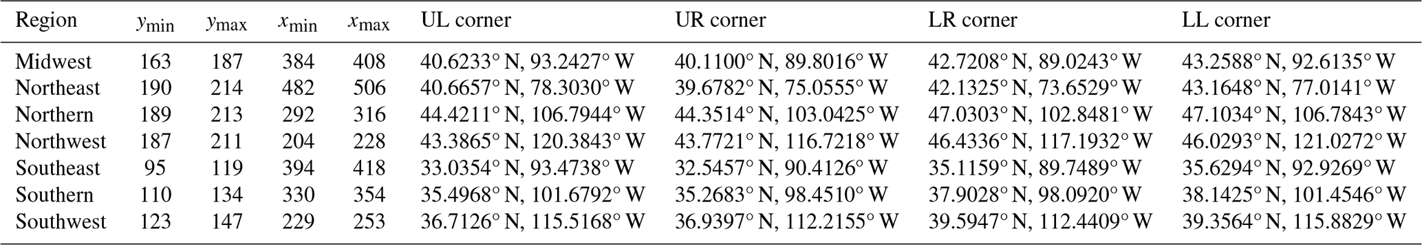
To assess the performance and generalizability of the proposed EMDBC method, we conducted a validation study using historical data from 1995 to 2004. This period was split into two parts: the first half (1995–1999) was used to develop and train our bias correction models, while the second half (2000–2004) was reserved for validation. The Livneh daily observed temperature series served as the reference dataset, and the EMDBC approach was applied to correct the daily temperature projections from CCSM. For a comprehensive spatial evaluation, we randomly selected seven areas, each measuring 25×25 grid cells (300 km × 300 km), from major subregions defined in the Fifth National Climate Assessment (USGCRP, 2023) across the continental United States, shown in Fig. 1, ensuring a diverse set of conditions. The seven areas are geographically defined in Appendix A.

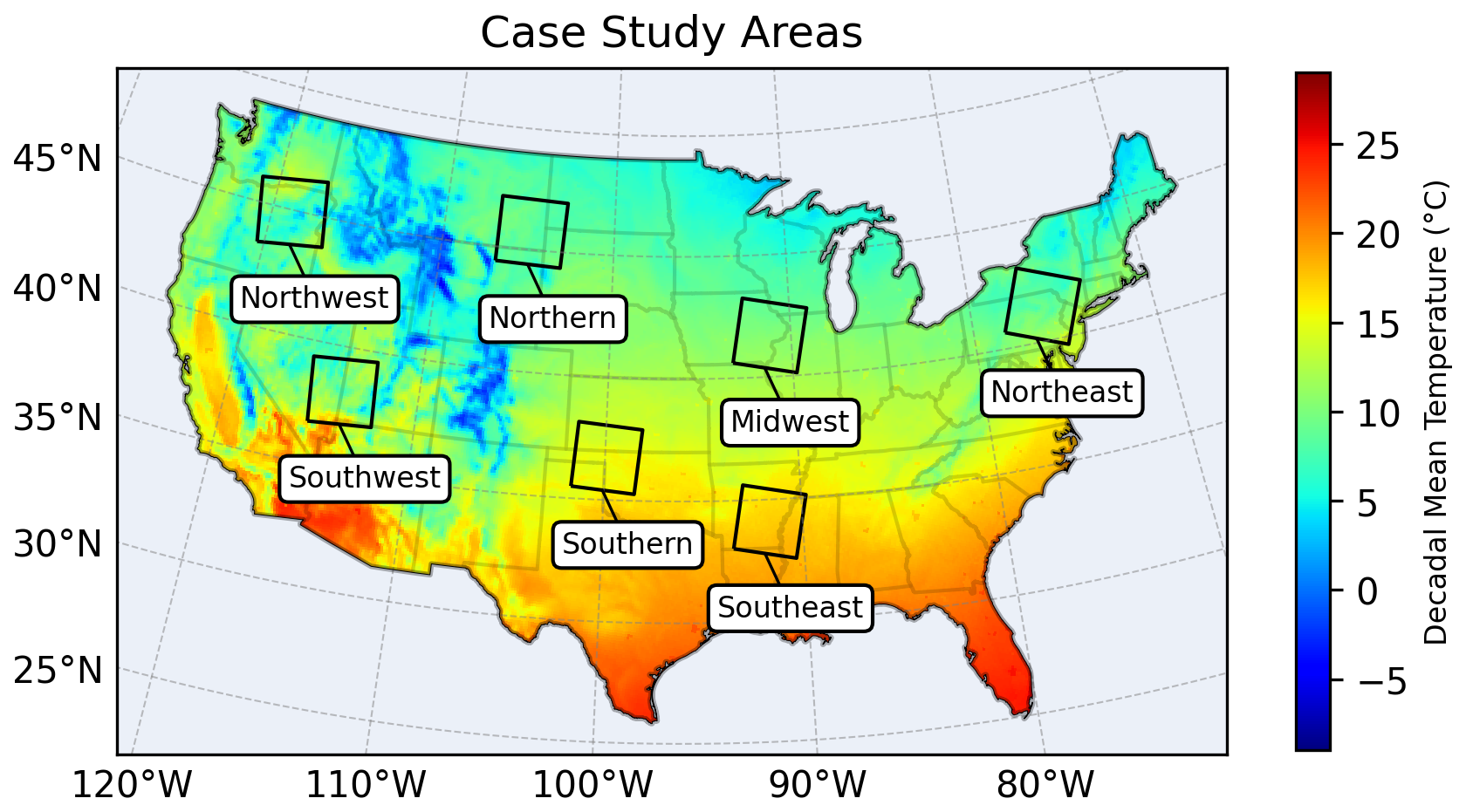
Figure 1 Map of case study regions selected for evaluating the bias correction methods. Boundaries are overlaid on the average 1995–2004 mean temperature field from WRF-CCSM, illustrating the diverse range of temperature regimes captured by the case study areas.

2.2 Quantile mapping-based bias adjustment

Quantile mapping (QM) is one of the most widely adopted bias correction (BC) techniques, designed to align the statistical distribution of model outputs with observations (see Chen et al., 2013 for a comprehensive review). By adjusting model outputs to match observed quantiles, QM can effectively reduce systematic biases related to both the central tendency and variability. Two prominent variants of this framework are briefly described below: Basic Quantile Mapping (QM) and Quantile Delta Mapping (QDM).

• Basic Quantile Mapping (QM): this approach directly corrects model outputs by aligning their quantile functions to that of the observed data (Tong et al., 2021; Kim et al., 2016). Let T_o the observed data, and $T_{\mathrm{p}}^{\mathrm{hist}}$ the historical model simulation. For a future model output $T_{\mathrm{p}}^{\mathrm{fut}}$, the bias-corrected value $T_{\mathrm{p}}^{\mathrm{fut},\mathrm{BC}}$ is given by:

  $$\begin{array}{}\text{(1)}& T_{\mathrm{p}}^{\mathrm{fut},\mathrm{BC}}=F_{\mathrm{o}}^{-\mathrm{1}}\left(F_{\mathrm{m}}^{\mathrm{hist}}\left(T_{\mathrm{p}}^{\mathrm{fut}}\right)\right),\end{array}$$

  where $F_{\mathrm{m}}^{\mathrm{hist}}$ is the empirical CDF of the model outputs in the historical period $T_{\mathrm{p}}^{\mathrm{hist}}$, and F_o is the empirical CDF of the observed data T_o. To bias-correct the future WRF–CCSM projections, we use the 1995–2004 Livneh observations as the calibration reference. Although QM ensures perfect distributional alignment for the historical period, it implicitly assumes that the observed CDF remains valid under future conditions – an assumption that can distort projected trends when the future outputs differs significantly from the historical weather regime.

• Quantile Delta Mapping (QDM): QDM extends QM by accounting for shifts between the historical and future model distributions (Tong et al., 2021; Maraun, 2016). Specifically, QDM maps future values $T_{\mathrm{p}}^{\mathrm{fut}}$ to their probabilities in both the future model CDF $F_{\mathrm{model}}^{\mathrm{fut}}$ and historical model CDF $F_{\mathrm{model}}^{\mathrm{hist}}$, then determines the corresponding quantiles in the observed CDF F_o. Finally, the difference (delta) between the historical and future mappings is added to the original future values. Mathematically, it can be written as:

  $$\begin{array}{}\text{(2)}& \begin{array}{rl}{T}_{\mathrm{p}}^{\mathrm{fut},\mathrm{bc}}& =F_{\mathrm{o}}^{-\mathrm{1}}\left(F_{\mathrm{p}}^{\mathrm{fut}}\left(T_{\mathrm{p}}^{\mathrm{fut}}\right)\right)\\ & +\left[T_{\mathrm{p}}^{\mathrm{fut}}-F_{\mathrm{p}}^{{\mathrm{hist}}^{-\mathrm{1}}}\left(F_{\mathrm{p}}^{\mathrm{fut}}\left(T_{\mathrm{p}}^{\mathrm{fut}}\right)\right)\right].\end{array}\end{array}$$

  This formulation permits future distributional changes to be incorporated into the bias correction. Various modifications, such as equidistant or equiratio quantile mapping (Li et al., 2010; Wang and Chen, 2014), have been shown to be mathematically equivalent to QDM (Cannon et al., 2015). In many applications involving large ranges (e.g., precipitation), the additive delta in Eq. (2) is replaced with a multiplicative factor. Nonparametric empirical CDFs are commonly used for flexibility, although parametric and semiparametric distributions can also be employed (Gudmundsson et al., 2012; Rajulapati and Papalexiou, 2023).

As highlighted in the introduction, QDM improves upon QM by allowing for distributional shifts from historical and future time periods. Nonetheless, most quantile-based methods effectively treat the entire time series on a single timescale, leaving biases at monthly, seasonal, or longer frequencies insufficiently addressed. This omission can result in residual errors that accumulate over extended periods, undermining confidence in long-term projections – a critical factor for both robust resilience assessments and strategic decision-making. These issues underscore the need for an approach that not only preserves the distributional changes in future projections but also captures timescale-dependent biases. In the next sections, we introduce the proposed EMDBC framework, which disentangles time-series of atmospheric variables produced by Earth system models into their intrinsic oscillatory modes. By applying tailored bias corrections to each timescale-specific component and subsequently recombining them, EMDBC aims to overcome the core limitations of QM and QDM, thereby offering a more robust and detailed method for bias correction in future projections.

2.3 Empirical mode decomposition and ensemble EMD

Empirical Mode Decomposition (EMD) (Huang et al., 1998) is a data-driven method to adaptively decompose a time series x(t) into a finite set of oscillatory components, called intrinsic mode functions (IMFs), plus a residual monotonic trend. Formally, EMD expresses a time series as:

$$\begin{array}{}\text{(3)}& x\left(t\right)=\sum _{i=\mathrm{1}}^n{c}_i\left(t\right)+r\left(t\right),\end{array}$$

where c_i(t) are the IMFs – each capturing variations over distinct timescales – and r(t) is the residual. Although EMD has found utility in diverse application domains, it can suffer from mode mixing, where oscillations of different frequencies end up blended in a single IMF.

To address this issue, Ensemble Empirical Mode Decomposition (EEMD) (Wu and Huang, 2009) was introduced. EEMD has been successfully incorporated in several recent studies, for example, Alizadeh et al. (2019), Kim et al. (2018), Liu et al. (2019) and Hawinkel et al. (2015). It adds multiple realizations of low-amplitude random noise, ϵ_j(t), to the original signal x(t) to form an ensemble of signals: $x_j\left(t\right)=x\left(t\right)+{\mathit{ϵ}}_j\left(t\right)$. EMD is then applied to each noise-added realization, and the resulting IMFs are averaged:

$$\begin{array}{}\text{(4)}& c_i^{\mathrm{EEMD}}\left(t\right)={\displaystyle \frac{\mathrm{1}}{N}}\sum _{j=\mathrm{1}}^N{c}_{i,j}\left(t\right),\end{array}$$

where c_i,j(t) denotes the ith IMF from the jth noise realization, and N is the ensemble size. By smoothing over numerous noise realizations, EEMD mitigates mode mixing, yielding a more robust and interpretable decomposition. This reliability is especially valuable for timescale-specific bias correction. We use the EEMD function available in the Python package PyEMD (Laszuk, 2017) to decompose temperature signals into IMFs.

2.4 EMD-based bias correction

Building on EEMD, we introduce an Empirical Mode Decomposition-based Bias Correction (EMDBC) framework for rectifying model biases across multiple timescales. As sketched in Fig. 2, EMDBC proceeds in three steps:

• i.

  timescale decomposition – the daily Livneh and CCSM series (Row 1) are split via EEMD into four bands (Rows 2–4);

• ii.

  timescale-specific correction – the residual and bi-weekly bands are adjusted with QDM, while the seasonal and annual bands use ensemble quantile regression (Row 5); and

• iii.

  reconstruction – the corrected bands are recombined to yield the final series for evaluation (Row 6).

We describe each of these steps in detail in the following subsections.

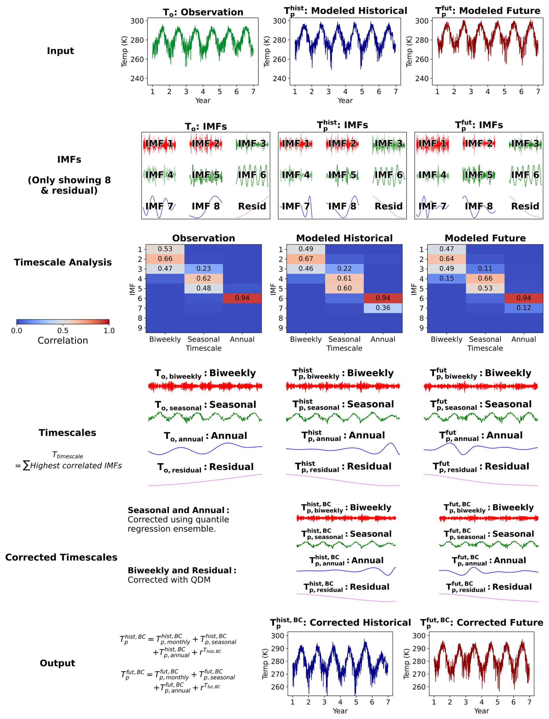
Figure 2 Timescale-wise bias correction framework using EMDBC. Three inputs are required: temperature timeseries from observation, modeled historical, and modeled future datasets. Here, to demonstrate EMDBC, timeseries data are extracted from Livneh (T_o), WRF-CCSM historical ($T_{\mathrm{p}}^{\mathrm{hist}}$), and WRF-CCSM mid-century ($T_{\mathrm{p}}^{\mathrm{fut}}$) at an arbitrary location. The input temperature series are decomposed into IMFs using EEMD. IMFs are then classified into predefined timescales: biweekly, seasonal, and annual. Bias correction is applied using QDM for biweekly timescale and residuals, and quantile regression for seasonal or annual timescales. Finally, the corrected timescales are summed to reconstruct the bias corrected temperature series.

2.4.1 Step 1: timescale decomposition

We begin by applying EEMD to decompose each time series into IMFs and a residual:

$$\begin{array}{}\text{(5)}& \begin{array}{rl}& T_{\mathrm{o}}=\sum _{j=\mathrm{1}}^{m^{T_{\mathrm{o}}}}{s}_j^{T_{\mathrm{o}}}+r^{T_{\mathrm{o}}},\\ & T_{\mathrm{p}}^{\mathrm{hist}}=\sum _{j=\mathrm{1}}^{m^{T_{\mathrm{p}}^{\mathrm{hist}}}}{s}_j^{T_{\mathrm{p}}^{\mathrm{hist}}}+r^{T_{\mathrm{p}}^{\mathrm{hist}}},\\ & T_{\mathrm{p}}^{\mathrm{fut}}=\sum _{j=\mathrm{1}}^{m^{T_{\mathrm{p}}^{\mathrm{fut}}}}{s}_j^{T_{\mathrm{p}}^{\mathrm{fut}}}+r^{T_{\mathrm{p}}^{\mathrm{fut}}}.\end{array}\end{array}$$

Here, T_o represents the observed series, $T_{\mathrm{p}}^{\mathrm{hist}}$ the historical model series, and $T_{\mathrm{p}}^{\mathrm{fut}}$ the future model series. For any given series s, the total number of extracted IMFs is m^s. Although EEMD generally reduces mode mixing, it may not fully ensure that each IMF corresponds to a unique frequency band. To address this, after each EEMD pass, we evaluate the peak frequency of every IMF, impose spacing constraints to minimize overlap, and iterate the decomposition with adjusted parameters until those constraints are satisfied. For the sake of clarity in presenting the timescale-wise bias correction, we have placed the detailed tuning procedure in Appendix B.

We then group these IMFs into broader frequency bands to reflect different timescales. For instance, the observed series T_o is aggregated as follows:

$$\begin{array}{}\text{(6)}& {\displaystyle }\begin{array}{rl}& T_{\mathrm{o},\mathrm{biweekly}}=\sum _{j=\mathrm{1}}^{\left[{\mathit{\tau }}_{\mathrm{1}}{m}^{T_{\mathrm{o}}}\right]}{s}_j^{T_{\mathrm{o}}},\\ & T_{\mathrm{o},\mathrm{seasonal}}=\sum _{j=\left[{\mathit{\tau }}_{\mathrm{1}}{m}^{T_{\mathrm{o}}}\right]+\mathrm{1}}^{\left[{\mathit{\tau }}_{\mathrm{2}}{m}^{T_{\mathrm{o}}}\right]}{s}_j^{T_{\mathrm{o}}},\\ & T_{\mathrm{o},\mathrm{annual}}=\sum _{j=\left[{\mathit{\tau }}_{\mathrm{2}}{m}^{T_{\mathrm{o}}}\right]+\mathrm{1}}^{m^{T_{\mathrm{o}}}}{s}_j^{T_{\mathrm{o}}},\end{array}\text{(7)}& {\displaystyle }{T}_{\mathrm{o}}=T_{\mathrm{o},\mathrm{biweekly}}+T_{\mathrm{o},\mathrm{seasonal}}+T_{\mathrm{o},\mathrm{annual}}+r^{T_{\mathrm{o}}}\end{array}$$

where $\mathrm{0}<{\mathit{\tau }}_{\mathrm{1}}<{\mathit{\tau }}_{\mathrm{2}}<\mathrm{1}$ are thresholds (often determined via bandpass or spectral methods) that separate biweekly, seasonal, and annual timescales. The biweekly band aggregates all IMFs with periods shorter than 14 d – thereby encapsulating the entire sub-daily to bi-weekly spectrum – while longer bands are formed by summing progressively lower-frequency IMFs. In this study, we perform bandpass filtering of the original signal, isolating the frequencies associated with each timescale using the butter function available in scipy (Virtanen et al., 2020). We then compute correlations between each IMF and each bandpass-filtered version of the signal, selecting τ₁ and τ₂ such that the IMFs most closely matching each frequency range are grouped together. For each IMF $s_j^{T_{\mathrm{o}}}$ we compute its Pearson correlation with the band-pass-filtered series representing the three target frequency ranges, denoted B₁ (bi-weekly), B₂ (seasonal), and B₃ (annual). Let

$$r_{j,k}=\mathrm{corr}\left(s_j^{T_{\mathrm{o}}},B_k\right),k\in \mathit{\{}\mathrm{1},\mathrm{2},\mathrm{3}\mathit{\}}.$$

Each IMF is assigned to the band for which the correlation is maximal, argmax_kr_j,k. Let $m^{T_{\mathrm{o}}}$ be the total number of IMFs for T_o. We define the cut-points

$$\begin{array}{ll}{\displaystyle }& {\displaystyle }{\mathit{\tau }}_{\mathrm{1}}={\displaystyle \frac{\max \left\{j:{\mathrm{argmax}}_k{r}_{j,k}=\mathrm{1}\right\}}{m^{T_{\mathrm{o}}}}},\\ {\displaystyle }& {\displaystyle }{\mathit{\tau }}_{\mathrm{2}}={\displaystyle \frac{\max \left\{j:{\mathrm{argmax}}_k{r}_{j,k}\le \mathrm{2}\right\}}{m^{T_{\mathrm{o}}}}},\end{array}$$

so $\lfloor {\mathit{\tau }}_{\mathrm{1}}{m}^{T_{\mathrm{o}}}\rfloor$ and $\lfloor {\mathit{\tau }}_{\mathrm{2}}{m}^{T_{\mathrm{o}}}\rfloor$ are the last indices assigned to the bi-weekly and seasonal groups, respectively. The same correlation-based scheme is applied to the IMFs of $T_{\mathrm{p}}^{\mathrm{hist}}$ and $T_{\mathrm{p}}^{\mathrm{fut}}$ to construct their corresponding time-scale bands. This step, illustrated in the “Timescale Analysis” portion of Fig. 2, organizes the IMFs into distinct frequency bands, laying the groundwork for applying the most suitable bias-correction strategy to each timescale in the subsequent steps.

2.4.2 Step 2: timescale-specific bias correction

Although each extracted frequency band represents the same underlying variable (e.g., temperature), the nature of the biases can vary greatly depending on whether we are dealing with short-term fluctuations (e.g., biweekly scales) or longer-term patterns (e.g., seasonal or annual). To address these differences, we apply distinct bias-correction strategies tailored to each frequency band, reflecting the idea that short-term extremes and variance require different treatments from slower, more systematic drifts or trends.

Biweekly component and residual trend

At the biweekly scale, signals often exhibit substantial variability and frequent extremes, yet show little in the way of stable temporal patterns that persist across years. Because a more complex regression approach is unlikely to provide significant benefits at this resolution, we use the QDM to correct these components. Likewise, the residual term – reflecting the underlying long-term trend – can also change considerably between observed and future periods. To capture these shifts and extremes effectively, we again use QDM, which directly infers quantiles from historical data while allowing for changes in the future distribution. Formally,

$$\begin{array}{}\text{(8)}& {\displaystyle }& {\displaystyle }{T}_{\mathrm{p},\mathrm{biweekly}}^{\mathrm{fut},\mathrm{BC}}=\mathrm{QDM}\left(T_{\mathrm{o},\mathrm{biweekly}},T_{\mathrm{p},\mathrm{biweekly}}^{\mathrm{hist}},T_{\mathrm{p},\mathrm{biweekly}}^{\mathrm{fut}}\right),\text{(9)}& {\displaystyle }& {\displaystyle }{r}^{T_{\mathrm{p}}^{\mathrm{fut},\mathrm{BC}}}=\mathrm{QDM}\left(r^{T_{\mathrm{o}}},r^{T_{\mathrm{p}}^{\mathrm{hist}}},r^{T_{\mathrm{p}}^{\mathrm{fut}}}\right).\end{array}$$

By aligning near-term fluctuations with observed quantiles, QDM preserves short-lived events and local variability without requiring additional predictors.

Seasonal and annual components

With daily-resolution data, longer timescales like seasons or years appear more structured, while shorter timescales show less pattern. Hence, for longer timescales, relying solely on QDM, an empirically driven method, may overlook structured variation better captured by predictor-based modeling. Consequently, we adopt a strategy that incorporates:

1. day: the day of the year, reflecting intra-annual variations,

2. $T_{\mathrm{p},\mathrm{long}}^{\mathrm{hist}}$: the model-simulated values aggregated at either the seasonal or annual scale, accounting for magnitude-dependent biases.

Let, $T_{\mathrm{p},\mathrm{long}}^{\mathrm{hist}}\in \mathit{\{}{T}_{\mathrm{p},\mathrm{seasonal}}^{hist},T_{\mathrm{p},\mathrm{annual}}^{\mathrm{hist}}\mathit{\}}$, $T_{\mathrm{p},\mathrm{long}}^{\mathrm{fut}}\in \mathit{\{}{T}_{\mathrm{p},\mathrm{seasonal}}^{fut},T_{\mathrm{p},\mathrm{annual}}^{\mathrm{fut}}\mathit{\}}$, $T_{\mathrm{o},\mathrm{long}}\in \mathit{\{}{T}_{\mathrm{o},\mathrm{seasonal}},T_{\mathrm{o},\mathrm{annual}}\mathit{\}}$, where each variable is a sum (or aggregation) of the IMFs corresponding to its relevant timescale. We define the historical bias as:

$${\mathrm{bias}}_{\mathrm{hist}}=T_{\mathrm{p},\mathrm{long}}^{\mathrm{hist}}-T_{\mathrm{o},\mathrm{long}},$$

and fit an ensemble of quantile regressions spanning a set of quantiles $\mathit{\{}{q}_{\mathrm{1}},q_{\mathrm{2}},\mathrm{\dots },q_{\mathrm{\ell }}\mathit{\}}$ (e.g., $q=\mathrm{0.05},\mathrm{0.06},\mathrm{\dots },\mathrm{0.99}$). For each quantile q_k, we train:

$$f_{q_k}\left(\mathrm{day},T_{\mathrm{p},\mathrm{long}}^{\mathrm{hist}}\right)={\widehat{\mathrm{bias}}}_{\mathrm{hist}}^{\left(q_k\right)},$$

capturing the bias at that particular quantile. The quantile regression analysis is performed using the QuantileRegressor model from scikit-learn – a Python library for machine learning (Pedregosa et al., 2011). When applied to future data, the same function yields

$${\widehat{\mathrm{bias}}}_{\mathrm{fut}}^{\left(q_k\right)}=f_{q_k}\left(\mathrm{day},T_{\mathrm{p},\mathrm{long}}^{\mathrm{fut}}\right).$$

We then correct the historical and future series accordingly:

$$T_{\mathrm{p},\mathrm{long}}^{\mathrm{hist},\mathrm{BC},\left(q_k\right)}=T_{\mathrm{p},\mathrm{long}}^{\mathrm{hist}}-{\widehat{\mathrm{bias}}}_{\mathrm{hist}}^{\left(q_k\right)},T_{\mathrm{p},\mathrm{long}}^{\mathrm{fut},\mathrm{BC},\left(q_k\right)}=T_{\mathrm{p},\mathrm{long}}^{\mathrm{fut}}-{\widehat{\mathrm{bias}}}_{\mathrm{fut}}^{\left(q_k\right)}.$$

Averaging the corrections across all ℓ quantiles produces the final bias-corrected data:

$$T_{\mathrm{p},\mathrm{long}}^{\mathrm{hist},\mathrm{BC}}={\displaystyle \frac{\mathrm{1}}{\mathrm{\ell }}}\sum _{k=\mathrm{1}}^{\mathrm{\ell }}{T}_{\mathrm{p},\mathrm{long}}^{\mathrm{hist},\mathrm{BC},\left(q_k\right)},T_{\mathrm{p},\mathrm{long}}^{\mathrm{fut},\mathrm{BC}}={\displaystyle \frac{\mathrm{1}}{\mathrm{\ell }}}\sum _{k=\mathrm{1}}^{\mathrm{\ell }}{T}_{\mathrm{p},\mathrm{long}}^{\mathrm{fut},\mathrm{BC},\left(q_k\right)}.$$

By leveraging multiple predictors and quantiles, this approach better encapsulates the full distribution – from lower tails to upper extremes – while also accounting for both seasonal cycles and magnitude-dependent biases. The result is a more nuanced and robust adjustment of long-term trends than would be possible using a single-quantile or purely empirical technique. timescales.

2.4.3 Step 3: reconstructing the corrected series

After bias-correcting each frequency band, we recombine them to form the final historical and future time series:

$$\begin{array}{}\text{(10)}& {\displaystyle }& {\displaystyle }{T}_{\mathrm{p}}^{\mathrm{hist},\mathrm{BC}}=T_{\mathrm{p},\mathrm{biweekly}}^{\mathrm{hist},\mathrm{BC}}+T_{\mathrm{p},\mathrm{seasonal}}^{\mathrm{hist},\mathrm{BC}}+T_{\mathrm{p},\mathrm{annual}}^{\mathrm{hist},\mathrm{BC}}+r^{T_{\mathrm{p}},\mathrm{BC}},\text{(11)}& {\displaystyle }& {\displaystyle }{T}_{\mathrm{p}}^{\mathrm{fut},\mathrm{BC}}=T_{\mathrm{p},\mathrm{biweekly}}^{\mathrm{fut},\mathrm{BC}}+T_{\mathrm{p},\mathrm{seasonal}}^{\mathrm{fut},\mathrm{BC}}+T_{\mathrm{p},\mathrm{annual}}^{\mathrm{fut},\mathrm{BC}}+r^{T_{\mathrm{p}},\mathrm{BC}}.\end{array}$$

Here, $T_{\mathrm{p},\mathrm{biweekly}}^{\mathrm{hist},\mathrm{BC}}$ and $T_{\mathrm{p},\mathrm{biweekly}}^{\mathrm{fut},\mathrm{BC}}$ denote the QDM-corrected short-term components, while $T_{\mathrm{p},\mathrm{seasonal}}^{\mathrm{hist},\mathrm{BC}}$ and $T_{\mathrm{p},\mathrm{annual}}^{\mathrm{hist},\mathrm{BC}}$ (along with their future counterparts) correspond to the multi-quantile regression corrections at longer timescales. The residual term $r^{T_{\mathrm{p}},\mathrm{BC}}$ is likewise corrected with QDM to address any leftover low-frequency bias.

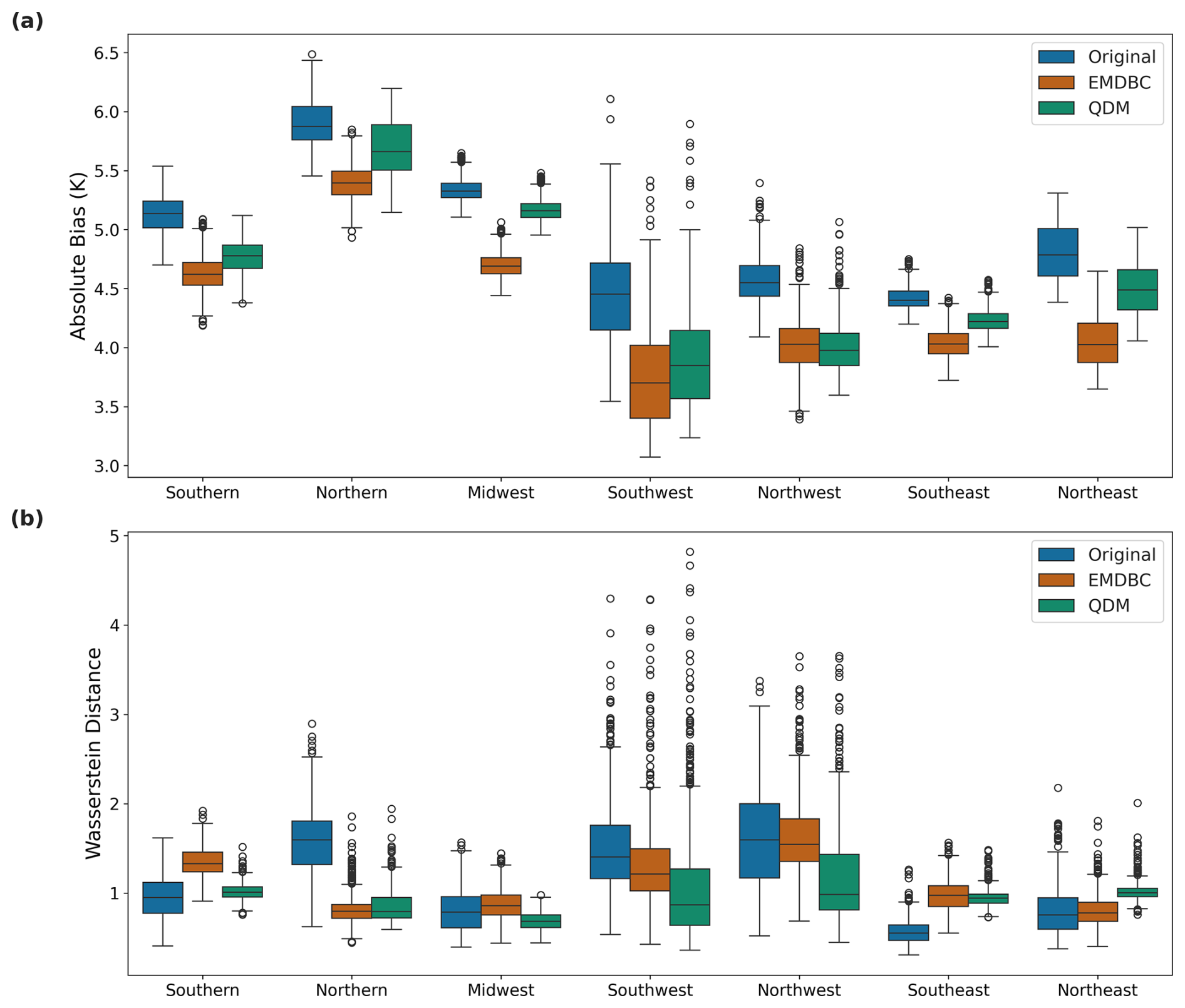
Figure 3 Comparison of Absolute Biases and Wasserstein Distances Across Sub-Regions in the original daily timescale. (a) Boxplots of the absolute temperature (in K) bias for the original (CCSM) and bias‐corrected (EMDBC and QDM) simulations across sub-regions on the validation dataset. (b) Boxplots of the corresponding Wasserstein distances between the observed and modeled temperature distributions across sub-regions on the validation dataset.

By integrating EEMD for timescale decomposition, QDM for high-frequency biases, and multi-quantile regression for seasonal to annual scales, the EMDBC framework provides a flexible and robust bias-correction method. It preserves both short-term fluctuations and long-term patterns, better handles extremes, and offers a more holistic view of uncertainty – addressing some of the most pressing gaps in conventional bias-correction approaches.

3 Results

This section describes the results from the validation study on seven case study areas and over the full domain. In both validation and full domain results, we apply a spatial smoothing procedure to the bias corrected daily temperature fields for both methods (QDM and EMDBC), while also censoring any values that exceed the original model's range to ensure numerical consistency and prevent unrealistic outliers. Since temperature typically exhibits strong spatial coherence, correcting each grid cell independently can introduce small-scale inconsistencies or artifacts. By averaging each cell's value with those of its immediate neighbors in a small 2D window (a 3×3 window in our experiments), we enhance local spatial continuity while preserving the broader-scale features necessary for downstream impact analyses. All visualization plots were generated using the matplotlib Python library (Hunter, 2007).

3.1 Validation results

Here, we include a comprehensive evaluation of traditional bias correction methods alongside our proposed approach. By applying the bias correction models to both the historical training scenario and the historical validation scenario, we can effectively assess each models ability to address biases and generalize across temporal scales where observed data does not exist (i.e., the future mid- and late century scenarios).

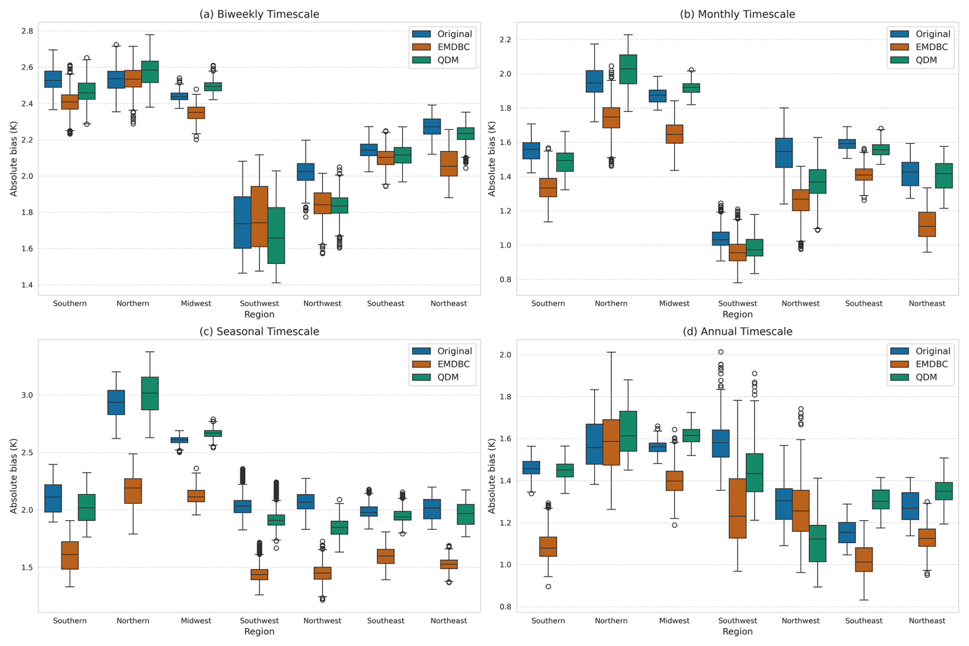
Figure 4 The timescale-wise average absolute bias per subregion on the validation dataset. Included timescapes are (a) biweekly, (b) monthly, (c) seasonal, and (d) annual.

We implement QDM and the proposed EMDBC to bias-correct the validation dataset introduced in Sect. 2.1. Figure 3 top panel shows the spatial distribution of the average absolute bias across these subregions and highlights the consistent performance gains achieved by EMDBC on held-out validation data. In addition, we examined the distributional similarity of the observed series and the model-projected series (both before and after bias correction) using the Wasserstein distance (WD). WD is defined as a distance between two probability measures P and Q on a metric space $(\mathcal{X},\Vert \cdot \Vert )$ by

$$\begin{array}{}\text{(12)}& W_{\mathrm{p}}(P,Q)={\left(\underset{\mathit{\gamma }\in \mathrm{\Gamma }(P,Q)}{inf}\underset{\mathcal{X}\times \mathcal{X}}{\int }\Vert x-y{\Vert }^{\mathrm{p}}\mathrm{d}\mathit{\gamma }(x,y)\right)}^{\mathrm{1}/p},\end{array}$$

where Γ(P,Q) denotes the set of all couplings with marginals P and Q; throughout this study we use the common choice p=1 (Panaretos and Zemel, 2019). Figure 3 down panel illustrates the WD across all subregions, demonstrating that the EMDBC correction preserves a distributional similarity to the observed series comparable to the QDM approach.

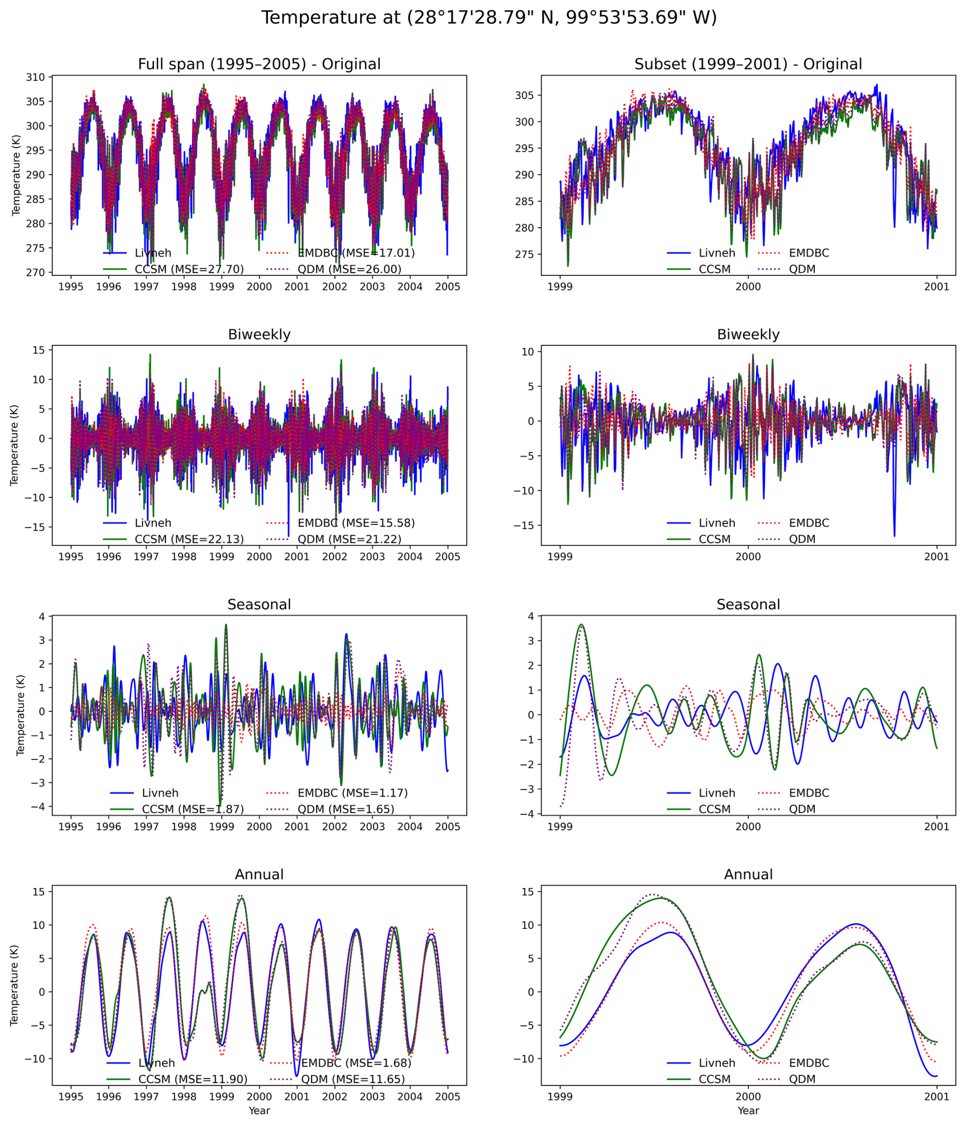
Figure 5 Bias-correction comparison across multiple time-scales at a representative grid cell. Column 1 shows the full 1995–2004 record, while Column 2 zooms into 1999–2001 for clarity. Solid lines correspond to the observed Livneh series (blue) and the raw CCSM projection (green); dashed lines show the bias-corrected outputs from EMDBC (red) and QDM (purple). Each row presents the original daily series and its bi-weekly, seasonal, and annual components, obtained by aggregating intrinsic mode functions as described in Sect. 2.4. The numbers at right report the mean-squared error (MSE, °K²) between each series and Livneh. While QDM matches EMDBC at the native daily scale, EMDBC yields consistently lower MSE at the bi-weekly, seasonal, and annual bands, indicating superior preservation of large-scale temperature variability.

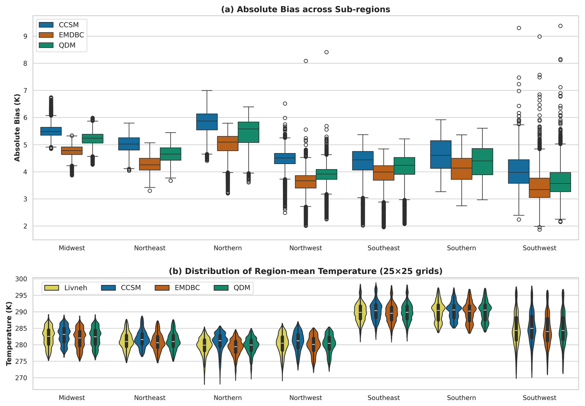
Figure 6 Comparison of CCSM Temperature Biases and Temperature Distributions Across Sub-Regions. (a) Boxplots of the absolute temperature bias before and after applying EMDBC and QDM corrections. (b) Violin plots showing the distribution of the average temperature for each sub-region.

Next, we assessed the performance of EMDBC at four distinct timescales – biweekly, monthly, seasonal, and half-annual – by comparing it to both QDM and the original CCSM output. To focus on each timescale, we used a Fast Fourier Transformation (FFT) based bandpass filtering method. First, the daily temperature series was transformed into the frequency domain. Then, all frequencies outside the target range were set to zero before an inverse transform was applied to reconstruct the filtered signal. This approach allowed us to isolate and compare how effectively each bias correction method captures variability at different temporal scales. Figure 4 shows the spatial distribution of the absolute bias across subregions for each filtered timescale. While EMDBC and QDM perform comparably at shorter timescales (biweekly), EMDBC demonstrates a progressively closer alignment with the observed series at longer timescales (monthly, seasonal, half-annual). Accurate bias correction at coarser temporal resolutions is especially important for large-scale resilience assessments and long-term planning, where cumulative effects and extended trends play a crucial role. This includes common uses cases of RCM and GCM, such as global, national, or regional impact studies (USGCRP, 2023); policy planning for risk assessment (Ranasinghe et al., 2021); energy infrastructure trends for long-term heating or cooling demands (Tan et al., 2023); drought security (Gamelin et al., 2022); agriculture planning (Jin et al., 2017); and understanding ecosystem biodiversity shifts (Liu et al., 2025). In other words, EMDBC shows promising ability to reduce temperature trend distortion caused by systematic biases due to model uncertainties and better capture temperature trend dynamics. This improved ability to preserve these longer-term patterns makes it a more reliable choice than QDM for applications that depend on consistent performance across multiple timescales.These results demonstrate that EMDBC successfully preserves bias-corrected signals over a broad range of temporal frequencies. By confirming EMDBC's effectiveness in an out-of-sample setting in this validation experiment, we gain confidence that it retains crucial physical relationships within the model more effectively than the traditional QDM, particularly at longer timescales. In the next section, we will evaluate its performance on the full GCM domain.

3.2 Over full domain

We apply EMDBC and QDM to the expanded model domain – covering all relevant time periods – to illustrate each method’s impact on temperature bias correction. As an initial illustration, Fig. 5 presents a single sampled location, decomposed in multiple timescales via the EMD-based approach described in Sect. 2.4. While QDM and EMDBC both perform well at the daily (training) scale, EMDBC more accurately preserves the longer-term fluctuations (e.g., seasonal and annual) seen in the observed Livneh data.

Turning next to broader spatial analyses, Fig. 6 focuses on various sub-regions across continental United States (CONUS). In each sub-region, the top panel compares the absolute temperature bias between the model projected and the observed series before and after correction with EMDBC and QDM, whereas the bottom panel shows the distribution of the average temperature. This figure demonstrates that EMDBC consistently reduces biases while maintaining an overall temperature distribution comparable to QDM.

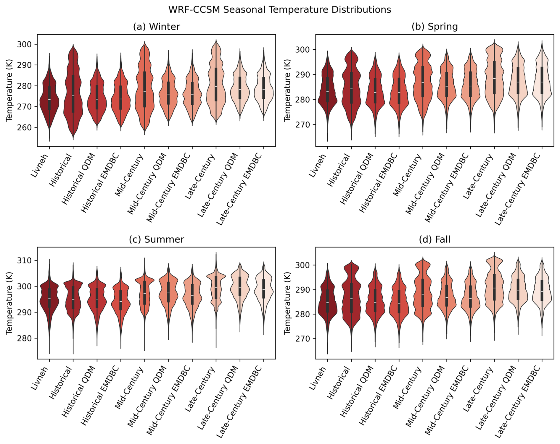
Figure 7 The mean daily temperature by season – (a) winter, (b) spring, (c) summer, (d) fall – across Livneh (1995–2004) and WRF-CCSM historical (1995–2004), mid-century (2045–2054), and late-century (2085–2094) timeframes before and after bias correction. Results for QDM and EMDBC are included. Violin plots displaying all timeframes on a common axis illustrate how both QDM and EMDBC preserve the shape of the observed spatial temperature distribution, while also showing the distribution's shift across centuries as projected by the WRF-CCSM model.

To verify whether these distributional consistencies hold across individual seasons, we next analyze Fig. 7, which illustrates the spatial distribution of seasonal-average temperature for the Livneh observations, the raw WRF-CCSM outputs, and their bias-corrected counterparts. At this aggregated seasonal level, both EMDBC and QDM move the model's temperature distribution closer to the observed data while retaining the overall projected warming trends through the mid- and late-century timeframes. This consistency further suggests that EMDBC not only reduces bias magnitude but also closely matches observed seasonal temperature patterns.

Finally, Figs. 9 and 8 show the average predicted daily bias (d–f) and the corresponding spatial maps ((g–i); e.g., annual or multi-year averages) for the raw and bias-corrected WRF-CCSM outputs. For reference, average Livneh observation data is also plotted, along with the average WRF-CCSM historical bias before and after correction (a–c). Here, “predicted bias” refers to the difference between the modeled temperature and its bias-corrected counterpart. EMDBC generally applies a stronger correction than QDM, resulting in slightly cooler daily temperature fields and a more uniform reduction of bias across the domain. Although we cannot fully validate future-period corrections in the absence of observations, EMDBC’s stronger alignment with historical data and its lower bias in validation sub-regions suggest it is well-equipped to handle changing conditions while preserving both short- and long-term temperature variability.

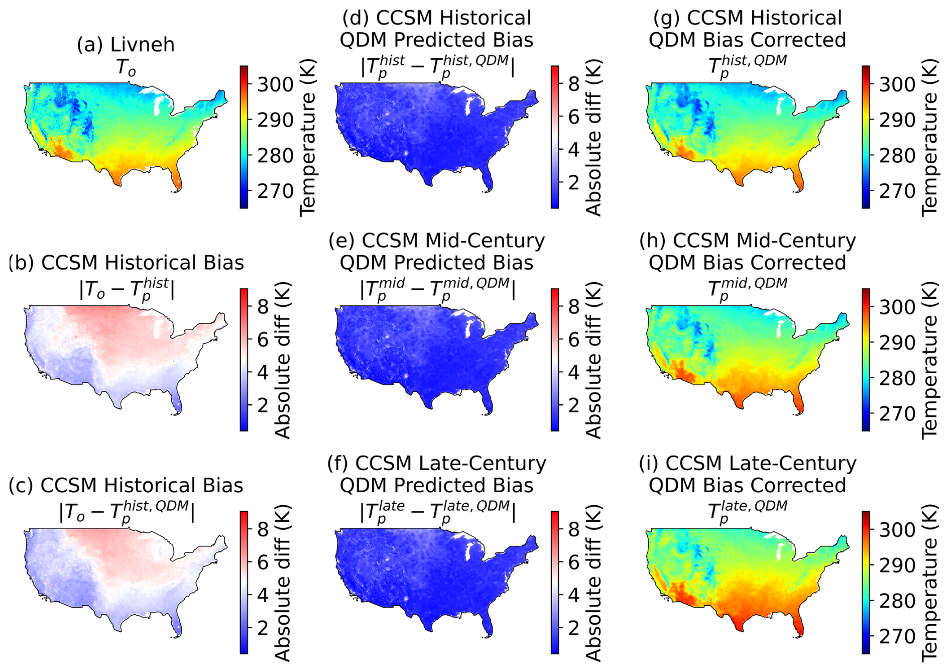
Figure 8 Temperature and temperature bias comparisons over CONUS before and after applying QDM. Left: (a) observed temperature (Livneh, 1995–2004), (b) WRF-CCSM historical (1995–2004) average daily absolute bias, and (c) QDM-corrected WRF-CCSM historical average daily absolute bias. Middle: (d) magnitude of QDM correction in historical, (e) mid-century (2045–2054), and (f) late-century (2085–2004) timeframes. Right: (g) QDM-corrected temperatures for WRF-CCSM historical, (h) mid-century, and (i) late-century periods.

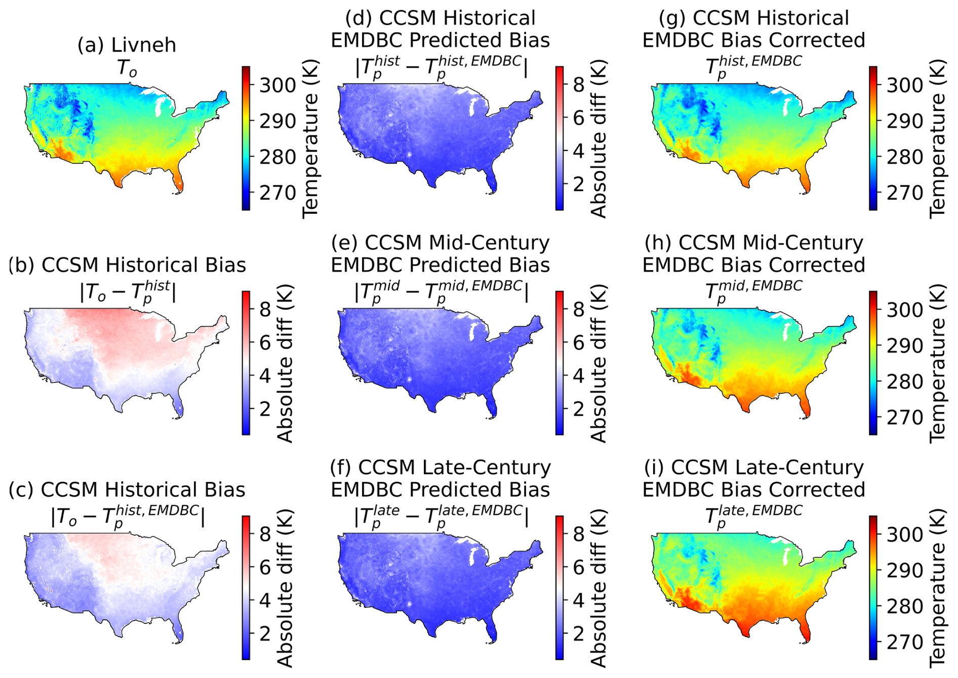
Figure 9 Temperature and temperature bias comparisons over CONUS before and after applying EMDBC. Left: (a) observed temperature (Livneh, 1995–2004), (b) WRF-CCSM historical (1995–2004) average daily absolute bias, and (c) EMDBC-corrected WRF-CCSM historical average daily absolute bias. Middle: (d) magnitude of EMDBC correction in historical, (e) mid-century (2045–2054), and (f) late-century (2085–2004) timeframes. Right: (g) EMDBC-corrected temperatures for WRF-CCSM historical, (h) mid-century, and (i) late-century periods.

4 Conclusion

This study proposes a new timescale-aware bias-correction methodology, EMDBC, and applies it to 12 km WRF-CCSM daily temperature simulations, covering historical (1995–2004), mid-century (2045–2054), and late-century (2085—094) periods across the contiguous United States. Furthermore, the EMDBC approach is validated by splitting historical model and observed data into training and validation sets and evaluating the validation set for bias reduction. In order to demonstrate the benefits of EMDBC, we compare the distributional similarities and absolute bias at varying timescales of the observed, model-projected, and bias corrected series. The results of this study highlight the importance of addressing biases across multiple timescales when correcting regional Earth system model outputs. Conventional approaches, such as mean-based linear scaling or quantile mapping, often focus on single distributions without adequately capturing longer-term fluctuations (e.g., monthly or seasonal). This limitation can lead to distorted trends and weakened physical consistency among atmospheric variables, thereby reducing confidence in model projections used for impact assessments and decision-making. In contrast, our EMDBC framework leverages Empirical Mode Decomposition (EMD) to isolate and correct distinct timescale wise oscillatory decomposition of a given signal, thereby preserving both short-term and long-term variability. Validation experiments show that EMDBC aligns better with observations at coarser temporal resolutions compared to conventional approaches, ensuring more accurate trends and enhanced physical consistency. These improvements are particularly relevant for applications where long-term signals – such as drought monitoring and risk assessment – play a critical role.

Nonetheless, several limitations remain. While the EMD decomposition offers theoretical guarantees for extracting intrinsic modes, segmenting them into discrete timescales still depends on user-defined thresholds, introducing a degree of subjectivity. A more rigorous, automated framework for determining these boundaries would further bolster EMDBC's robustness. Additionally, although ensemble EMD (EEMD) helps mitigate mode mixing, more advanced signal-processing or machine learning techniques could optimize the decomposition process. Another promising avenue for future work is the exploration of multivariate EMD approaches, which would facilitate a more comprehensive bias correction by preserving inter-variable dependencies among variable fields. Despite these open questions, our results demonstrate that a timescale-aware bias-correction strategy significantly enhances model projection reliability and paves the way for continued innovation in this area.

Appendix A: Case study regions used in validation

Table A1 Bounding-box definitions for each case-study region. Columns y_min, y_max, x_min, and x_max list the 0-based Python array indices that isolate the region within the WRF domain supplied with the dataset linked in the data availability statement; the remaining columns give the decimal-degree latitudes and longitudes of the four bounding-box corners: upper left (UL), upper right (UR), lower right (LR), and lower left (LL).

Appendix B: Optimal tuning of IMFs for EMDBC

The performance of the proposed EMDBC framework depends on the quality and separation of the IMFs generated during the decomposition process. A common challenge in EMD methods is mode-mixing, where oscillatory modes of different frequencies are entangled within a single IMF, reducing interpretability and effectiveness (Tang et al., 2012). While the Ensemble EMD (EEMD) approach (Wu and Huang, 2009) mitigates mode-mixing by introducing random noise, it does not fully eliminate the issue. Several alternative strategies have been proposed to ensure distinct frequency bands for IMFs (Tang et al., 2012; Fosso and Molinas, 2018), but none has proven universally robust.

To address the instability of IMFs and ensure their meaningful separation across timescales, we impose constraints on their maximum amplitude frequencies (f_max) calculated using the Fast Fourier Transform (FFT) (Rockmore, 2000). This process is iterative: IMFs are generated, evaluated against the constraints, and refined until all conditions are satisfied. The constraints are defined as follows:

• Ensuring distinct timescales: each IMF must represent a unique timescale, maintaining a strictly decreasing frequency trend:

  $$\mathrm{\Delta }{f}_{\max }^{\left(j\right)}=f_{\max }^{\left(j\right)}-f_{\max }^{(j+\mathrm{1})}>\mathrm{0},\forall j,$$

  where $f_{\max }^{\left(j\right)}$ denotes the maximum amplitude frequency of the jth IMF.

• Preventing overlap: to avoid redundancy, the relative change in frequency between consecutive IMFs must exceed a minimum threshold:

  $${\displaystyle \frac{\mathrm{\Delta }{f}_{\max }^{\left(j\right)}}{f_{\max }^{\left(j\right)}}}>{\mathit{\delta }}_{\min }.$$

• Maintaining regularity: the progression of frequencies across IMFs should be smooth, avoiding abrupt changes. This is enforced by ensuring:

  $$\begin{array}{}\text{(B1)}& {\displaystyle \frac{\mathrm{\Delta }{f}_{\max }^{\left(j\right)}}{f_{\max }^{\left(j\right)}}}<{\mathit{\delta }}_{\max }.\end{array}$$

The thresholds δ_min and δ_max act as hyperparameters, which can be tuned through cross-validation. In our experiments, setting δ_min=0.2 and δ_max=0.8 yielded satisfactory results. The algorithm iteratively checks these constraints after each generation of IMFs. If all conditions are satisfied, the process terminates; otherwise, new IMFs are generated, and the constraints are re-evaluated. The following algorithm outlines the major steps in this iterative optimization process:

By iteratively applying these constraints, we ensure that the IMFs represent distinct timescales, avoid redundancy, and maintain smooth frequency progression. This optimization significantly enhances the stability of the decomposition and improves the effectiveness of EMDBC in handling challenging cases of mode-mixing or overlapping frequency bands.

Algorithm B1 Iterative Optimization of IMFs for EMDBC.

1:

Input: time series x(t), thresholds δ_min, δ_max

2:

Output: optimized set of IMFs, $\mathit{\{}{s}_j{\mathit{\}}}_{j=\mathrm{1}}^m$

3:

Initialize: generate initial IMFs using EEMD: $\mathit{\{}{s}_j{\mathit{\}}}_{j=\mathrm{1}}^m$

4:

Compute maximum amplitude frequencies $f_{\max }^{\left(j\right)}$ using FFT

5:

while any constraint is violated do

6:

Check distinct timescales: $\mathrm{\Delta }{f}_{\max }^{\left(j\right)}>\mathrm{0},\forall j$

7:

Check overlap: $\frac{\mathrm{\Delta }{f}_{\max }^{\left(j\right)}}{f_{\max }^{\left(j\right)}}>{\mathit{\delta }}_{\min }$

8:

Check regularity: $\frac{\mathrm{\Delta }{f}_{\max }^{\left(j\right)}}{f_{\max }^{\left(j\right)}}<{\mathit{\delta }}_{\max }$

9:

if any condition is violated then

10:

Regenerate IMFs using updated parameters

11:

Recompute $f_{\max }^{\left(j\right)}$

12:

end if

13:

end while

14:

return  Optimized $\mathit{\{}{s}_j{\mathit{\}}}_{j=\mathrm{1}}^m$

Appendix C: Description of the acronyms

Table C1 Acronyms and Symbols used in this study.