HOPE: an arbitrary-order non-oscillatory finite-volume shallow water dynamical core with automatic differentiation

This study presents the High Order Prediction Environment (HOPE), an automatically differentiable, non-oscillatory finite-volume dynamical core for shallow water equations on the cubed-sphere grid. HOPE integrates five key features: (1) arbitrary high-order accuracy through genuine two-dimensional reconstruction schemes; (2) essential non-oscillation via adaptive polynomial order reduction in discontinuous regions; (3) exact mass conservation inherited from finite-volume discretization; (4) automatically differentiable and (5) GPU-native scalability through PyTorch-based implementation. Another innovation is the development of a two-way coupled ghost cell interpolation method. This approach incorporates information from adjacent panels on both sides of the boundary, thereby overcoming the integration instability inherent in one-sided ghost cell interpolation approaches when using high-order reconstruction. Leveraging the linear operator nature of this interpolation scheme, we optimized its computation: information exchange across the panel boundary is achieved through a single matrix-vector multiplication instead of iterative coupling, without accuracy loss. Numerical experiments demonstrate the capabilities of HOPE: The 11th-order scheme reduces errors to near double-precision round-off levels in steady-state geostrophic flow tests on coarse grids. Maintenance of Rossby–Haurwitz waves over 100 simulation days without crashing. A cylindrical dam-break test case confirms the genuinely two-dimensional WENO scheme exhibits significantly better isotropy compared to dimension-by-dimension approaches. Moreover, normalized conservation errors in total energy, total potential enstrophy, and total zonal angular momentum significantly reduce with increasing order of the reconstruction scheme. Two implementations are developed: a Fortran version for convergence analysis and a PyTorch version leveraging automatic differentiation and GPU acceleration. The PyTorch implementation maps reconstruction and quadrature operation to 2D convolution and Einstein summation respectively, achieving about 2× speedup on single NVIDIA RTX3090 GPU versus Dual Intel E5-2699v4 CPUs execution. This design enables seamless coupling with neural network parameterizations, positioning HOPE as a foundational tool for next-generation differentiable atmosphere models.

1 Introduction

Recent years have witnessed a surge in research integrating numerical weather prediction (NWP) with artificial intelligence (AI) techniques. A prominent advancement in this domain is the hybrid modeling paradigm, which synergizes the complementary strengths of both approaches. This framework implements numerical dynamical cores within AI software platforms such as TensorFlow or PyTorch, thereby enabling seamless integration of AI models into the numerical solution process for atmospheric dynamical partial differential equations (PDEs). Unlike the fully surrogated methods, such as Pangu-Weather (Bi et al., 2022), FengWu (Chen et al., 2023), GraphCast (Lam et al., 2023), NowcastNet (Zhang et al., 2023), hybrid model integrates traditional PDE-based dynamical cores with neural network (NN)-based physical parameterizations. The auto-differentiable nature of the dynamical core enables training losses to propagate through the entire model during backpropagation, allowing the NN-based parameterization module to access more comprehensive residual information. NeuralGCM (Kochkov et al., 2024) exemplifies this hybrid approach by combining a spectral numerical dynamical core with NN-based physical parameterizations. The governing equation-based dynamical core imposes rigorous physical constraints within the framework, effectively mitigating the blurriness characteristic of purely data-driven models. Furthermore, NeuralGCM demonstrates superior power spectra performance compared to conventional data-driven meteorological models. While the implementation of a spectral dynamical core in NeuralGCM theoretically enables infinite-order accuracy, the global nature of spectral expansion restricts the method's scalability. Furthermore, in contrast to finite-volume algorithms which inherently ensure strict mass conservation, achieving strict mass conservation with NeuralGCM's spectral dynamical core requires supplementary modifications.

To address these shortcomings, we present the High Order Prediction Environment (HOPE) dynamical core with following contributions:

1. A new-generation shallow-water model architecture integrating:

   • i.

     Arbitrary high-order accuracy (up to 13th-order verified) via tensor product polynomial (TPP).

   • ii.

     A finite-volume scheme requiring only information from a local stencil surrounding each cell to perform state updates, enabling massively parallel scalability.

   • iii.

     Inherent mass conservation from finite-volume discretization.

   • iv.

     A WENO (Weighted Essentially Non-Oscillatory) based, adaptive polynomial order reduction for essential non-oscillation.

2. A novel two-way coupled ghost cell interpolation scheme achieving:

   • i.

     Arbitrary odd-order convergence through central stencil interpolation.

   • ii.

     Single sparse matrix-vector operation replacing iterative procedures (Eq. A.12).

   • iii.

     Overcome numerical instability beyond 7th-order accuracy.

3. PyTorch-based high performance differentiable implementation featuring:

   • i.

     GPU acceleration through convolution/einsum operator in PyTorch, 2× speedup on single RTX3090 GPU vs. Dual Intel Xeon 2699v4 CPUs.

   • ii.

     Automatic ghost cell interpolation matrix generation via native auto-differentiation.

   • iii.

     Seamless integration with NN modules for hybrid modeling.

In the following part of the introduction, we introduce the relevant work on constructing the HOPE model, and from this, we elaborate on the challenges and motivations for establishing the algorithm of the dynamical core. High-order accuracy is an extremely appealing trait for the design of a dynamical core, particularly in high-resolution atmospheric simulations. A dynamical core model with high-order accuracy produces significantly less simulation error in smooth regions compared to a low-order model. Furthermore, even when the resolution is equivalent or coarser, a high-order model is capable of resolving finer details than a low-order one.

A high-order finite volume model was developed on cubed sphere, named MCORE (Ullrich et al., 2010; Ullrich and Jablonowski, 2012). High-order reconstruction requires information from cells external to panel boundaries (commonly termed ghost cells). Due to coordinate discontinuities across the six panels of the cubed-sphere grid, MCORE implements an interpolation scheme for ghost cells based on one-side information. This approach employs a two-dimensional reconstruction stencil to interpolate prognostic variables onto Gaussian quadrature points within each cell, followed by integration to obtain cell-averaged values. The authors assert that MCORE's convergence rate can theoretically be of arbitrary order. However, during the design of the ghost cell interpolation for HOPE, we initially attempted to use a one-sided reconstruction stencil similar to MCORE. While stable integration was achieved with the 3rd-, 5th-, and 7th-order schemes, the model became unstable when schemes of 9th-order or higher were used. In other words, for HOPE, overcoming the 7th-order accuracy limitation necessitated the development of a new ghost cell interpolation scheme.

Therefore, we designed a bilateral interpolation algorithm. This algorithm employs an iterative procedure that incorporates information from both adjacent panels of the cubed-sphere grid simultaneously. This enabled stable model integration even with higher-order schemes. Though not detailed in the paper, our testing confirmed stable integration even at 13th-order accuracy.

In this article, we devise the reconstruction based on tensor product polynomial (TPP). When the stencil width is k, our method achieves kth order accuracy, surpassing MCORE by one order of accuracy with the same stencil width. In addition, we have developed a new class of ghost interpolation schemes that abandon the use of one-sided stencils and instead adopt central stencils. This new approach enables the scheme to overcome the non-physical oscillations arising from interpolation at panel boundaries. Our method allows for arbitrary order of accuracy while the field is smooth enough, and we have verified this by testing up to the 11th order.

Nevertheless, higher-order reconstruction does not invariably yield superior simulation outcomes, as elucidated by analyzing the properties of the Taylor series remainder term. The accuracy of approximating a function via a Taylor series requires two essential conditions: (1) the existence of higher-order derivatives of the function at the expansion point, and (2) the convergence of the series within the relevant domain. When the field exhibits poor continuity – where higher-order derivatives either do not exist or lead to increasing residuals with series order – employing higher-order approximations can introduce significant errors. Therefore, for reconstruction schemes based on polynomial functions, high-order accuracy should only be adopted when the field is sufficiently smooth. Conversely, for discontinuous or poorly continuous fields, reducing the reconstruction order is necessary to maintain numerical stability and effectiveness.

The Weighted Essentially Non-Oscillatory (WENO) scheme is an adaptive limiter widely employed in computational fluid dynamics (CFD) to address this challenge. Originally developed for one-dimensional problems (Liu et al., 1994), WENO was later extended to two dimensions by Shi et al. (2002) using two distinct approaches: a genuinely two-dimensional (WENO2D) scheme and a dimension-by-dimension reconstruction. In this work, we implement WENO2D scheme to enforce the non-oscillatory property. This approach effectively suppresses non-physical oscillations near sharp discontinuities while preserving high-order accuracy in smooth regions.

The remainder of this paper is organized as follows: Sect. 2 details the governing equations on the cubed-sphere grid. Section 3 presents the numerical methods, including reconstruction schemes, panel boundary treatment method, and temporal marching scheme. Section 4 focuses on HOPE's high-performance implementation leveraging PyTorch's built-in operators for GPU acceleration. The adoption of PyTorch simultaneously enables automatic differentiation capabilities through its computational graph construction. Section 5 validates model performance through standard test cases, followed by conclusions and future directions in Sect. 6.

2 Governing equation on cubed sphere

The cubed-sphere grid partitions the spherical domain into six panels, each with a structured and rectangular computational space. This configuration facilitates high-order spatial reconstruction and efficient massive-thread parallelism (see Fig. 1). Early work on solving the primitive equations on the cubed-sphere grid dates back to Sadourny (1972). In recent decades, the cubed-sphere grid has been widely adopted in high-order-accuracy atmospheric models. For instance, Chen and Xiao (2008) developed a shallow water model using the multi-moment constrained finite volume method on the cubed sphere, achieving 3rd–4th order accuracy. Ullrich et al. (2010) designed a high-order finite volume dynamical core based on this grid, Nair et al. (2005a, b) implemented a discontinuous Galerkin model on the cubed sphere.

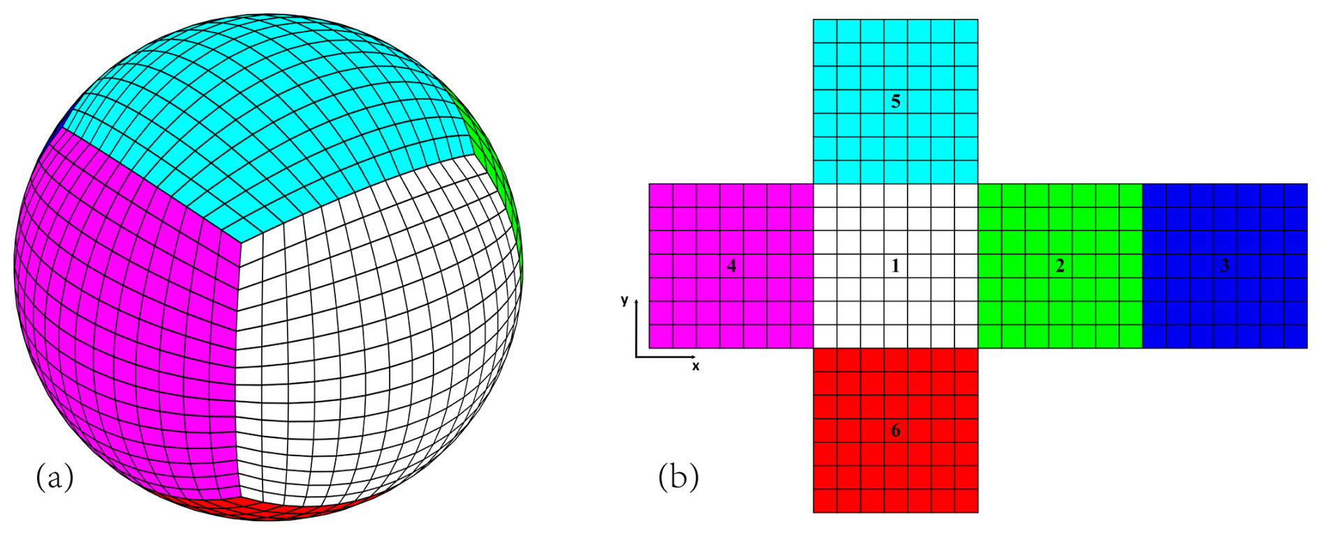
Figure 1 Cubed sphere grid. (a) Physical space; (b) computational space. Six panels are identified by indices from 1 to 6.

In this study, we also employ the equiangular cubed-sphere grid. Although the mesh is non-orthogonal, the computational space can still be treated as a rectangular grid by adopting a generalized curvilinear coordinate system. In this section, we present the shallow water equations in generalized curvilinear coordinates and discuss specialized treatments for topography.

Shallow water equation set on gnomonic equiangular cubed sphere grid is written as

$$\begin{array}{}\text{(1)}& \left\{\begin{array}{l}\frac{\partial \sqrt{G}\mathit{\varphi }}{\partial t}+\frac{\partial \sqrt{G}\mathit{\varphi }u}{\partial x}+\frac{\partial \sqrt{G}\mathit{\varphi }v}{\partial y}=\mathrm{0}\\ \frac{\partial \sqrt{G}\mathit{\varphi }u}{\partial t}+\frac{\partial \sqrt{G}\left(\mathit{\varphi }uu+\frac{\mathrm{1}}{\mathrm{2}}{G}^{\mathrm{11}}{\mathit{\varphi }}^{\mathrm{2}}\right)}{\partial x}+\frac{\partial \sqrt{G}\left(\mathit{\varphi }uv+\frac{\mathrm{1}}{\mathrm{2}}{G}^{\mathrm{12}}{\mathit{\varphi }}^{\mathrm{2}}\right)}{\partial y}={\mathit{\psi }}_{\mathrm{M}}^{\mathrm{1}}+{\mathit{\psi }}_{\mathrm{C}}^{\mathrm{1}}+{\mathit{\psi }}_{\mathrm{B}}^{\mathrm{1}}\\ \frac{\partial \sqrt{G}\mathit{\varphi }v}{\partial t}+\frac{\partial \sqrt{G}\left(\mathit{\varphi }uv+\frac{\mathrm{1}}{\mathrm{2}}{G}^{\mathrm{21}}{\mathit{\varphi }}^{\mathrm{2}}\right)}{\partial x}+\frac{\partial \sqrt{G}\left(\mathit{\varphi }vv+\frac{\mathrm{1}}{\mathrm{2}}{G}^{\mathrm{22}}{\mathit{\varphi }}^{\mathrm{2}}\right)}{\partial y}={\mathit{\psi }}_{\mathrm{M}}^{\mathrm{2}}+{\mathit{\psi }}_{\mathrm{C}}^{\mathrm{2}}+{\mathit{\psi }}_{\mathrm{B}}^{\mathrm{2}}\end{array}\right..\end{array}$$

The gnomonic equiangular coordinates are represented by (x, y, p), where $(x,y)\in \left[-\frac{\mathit{\pi }}{\mathrm{4}},\frac{\mathit{\pi }}{\mathrm{4}}\right]$ are local equiangular coordinate of each panel and p=1, 2, 3, …, n_p is panel index as shown in Fig. 1b; n_p=6 is the number of panels. ϕ=gh is geopotential, h is fluid thickness, u and v are the contravariant wind components in the x and y directions, respectively, g is gravity acceleration. ψ_M, ψ_C, ψ_B are the metric term, Coriolis term and bottom topography influence term

$$\begin{array}{}\text{(2)}& {\displaystyle }\begin{array}{rl}{\mathit{\psi }}_{\mathrm{M}}=& \left(\begin{array}{c}{\mathit{\psi }}_{\mathrm{M}}^{\mathrm{1}}\\ {\mathit{\psi }}_{\mathrm{M}}^{\mathrm{2}}\end{array}\right)={\displaystyle \frac{\mathrm{2}\sqrt{G}}{{\mathit{\delta }}^{\mathrm{2}}}}\\ & \left(\begin{array}{l}-X{Y}^{\mathrm{2}}\mathit{\varphi }uu+Y\left(\mathrm{1}+Y^{\mathrm{2}}\right)\mathit{\varphi }uv\\ X\left(\mathrm{1}+X^{\mathrm{2}}\right)\mathit{\varphi }uv-X^{\mathrm{2}}Y\mathit{\varphi }vv\end{array}\right)\end{array}\text{(3)}& {\displaystyle }\begin{array}{rl}{\mathit{\psi }}_{\mathrm{C}}=& -\sqrt{G}\sqrt{G}f\mathbf{k}\times \mathit{\varphi }\mathbf{u}=\sqrt{G}f\left(\begin{array}{cc}-G^{\mathrm{12}}& G^{\mathrm{11}}\\ -G^{\mathrm{22}}& G^{\mathrm{12}}\end{array}\right)\\ & \left(\begin{array}{c}\sqrt{G}\mathit{\varphi }u\\ \sqrt{G}\mathit{\varphi }v\end{array}\right)\end{array}\text{(4)}& {\displaystyle }{\mathit{\psi }}_{\mathrm{B}}=-\sqrt{G}\mathit{\varphi }{G}^{ij}{\displaystyle \frac{\partial {\mathit{\varphi }}_{\mathrm{s}}}{\partial x^j}}=-\sqrt{G}\mathit{\varphi }\left(\begin{array}{c}{G}^{\mathrm{11}}\frac{\partial {\mathit{\varphi }}_{\mathrm{s}}}{\partial x}+G^{\mathrm{12}}\frac{\partial {\mathit{\varphi }}_{\mathrm{s}}}{\partial y}\\ G^{\mathrm{21}}\frac{\partial {\mathit{\varphi }}_{\mathrm{s}}}{\partial x}+G^{\mathrm{22}}\frac{\partial {\mathit{\varphi }}_{\mathrm{s}}}{\partial y}\end{array}\right)\end{array}$$

where $X=\tan x,Y=\tan y,\mathit{\delta }=\sqrt{\mathrm{1}+X^{\mathrm{2}}+Y^{\mathrm{2}}}$, f=2Ωsin θ is Coriolis parameter, ϕ_s=gh_s is surface geopotential, and h_s is surface height.

$$\begin{array}{}\text{(5)}& \sin \mathit{\theta }=\left\{\begin{array}{ll}Y/\mathit{\delta },& p\in \mathit{\{}\mathrm{1},\mathrm{2},\mathrm{3},\mathrm{4}\mathit{\}}\\ \mathrm{1}/\mathit{\delta },& p=\mathrm{5}\\ -\mathrm{1}/\mathit{\delta },& p=\mathrm{6}\end{array}\right.\end{array}$$

The contravariant metric on cubed-sphere is

$$\begin{array}{}\text{(6)}& G^{ij}={\displaystyle \frac{{\mathit{\delta }}^{\mathrm{2}}}{r^{\mathrm{2}}\left(\mathrm{1}+X^{\mathrm{2}}\right)\left(\mathrm{1}+X^{\mathrm{2}}\right)}}\left(\begin{array}{ll}\mathrm{1}+Y^{\mathrm{2}}& XY\\ XY& \mathrm{1}+X^{\mathrm{2}}\end{array}\right).\end{array}$$

The covariant metric

$$\begin{array}{}\text{(7)}& G_{ij}={\displaystyle \frac{r^{\mathrm{2}}\left(\mathrm{1}+X^{\mathrm{2}}\right)\left(\mathrm{1}+Y^{\mathrm{2}}\right)}{{\mathit{\delta }}^{\mathrm{4}}}}\left(\begin{array}{ll}\mathrm{1}+X^{\mathrm{2}}& -XY\\ -XY& \mathrm{1}+Y^{\mathrm{2}}\end{array}\right)\end{array}$$

and the metric determinant is given by

$$\begin{array}{}\text{(8)}& \sqrt{G}=\sqrt{\det \left(G_{ij}\right)}={\displaystyle \frac{r^{\mathrm{2}}\left(\mathrm{1}+X^{\mathrm{2}}\right)\left(\mathrm{1}+Y^{\mathrm{2}}\right)}{{\mathit{\delta }}^{\mathrm{3}}}}.\end{array}$$

r is radius of earth.

The contravariant wind vector $\mathit{V}=(u,v)$ can be convert to wind vector on spherical LAT/LON coordinate ${\mathit{V}}_{\mathrm{s}}=(u_{\mathrm{s}},v_{\mathrm{s}})$ by the following formula

$$\begin{array}{}\text{(9)}& \left(\begin{array}{c}{u}_{\mathrm{s}}\\ v_{\mathrm{s}}\end{array}\right)=\mathbf{J}\left(\begin{array}{c}u\\ v\end{array}\right)\end{array}$$

where J is a 2×2 conversion matrix, the expressions are different in each panel

$$\begin{array}{}\text{(10)}& {\displaystyle }\begin{array}{rl}& \mathbf{J}=r\left(\begin{array}{ll}\cos \mathit{\theta }\frac{\partial \mathit{\lambda }}{\partial x}& \cos \mathit{\theta }\frac{\partial \mathit{\lambda }}{\partial y}\\ \frac{\partial \mathit{\theta }}{\partial x}& \frac{\partial \mathit{\theta }}{\partial y}\end{array}\right)=\\ & \left\{\begin{array}{l}r\left(\begin{array}{ll}\cos \mathit{\theta }& \mathrm{0}\\ -\sin \mathit{\theta }\cos \mathit{\theta }\tan {\mathit{\lambda }}_p& \cos {\mathit{\lambda }}_p{\cos }^{\mathrm{2}}\mathit{\theta }+\frac{{\sin }^{\mathrm{2}}\mathit{\theta }}{\cos {\mathit{\lambda }}_p}\end{array}\right),p\in \mathit{\{}\mathrm{1},\mathrm{2},\mathrm{3},\mathrm{4}\mathit{\}}\\ r\left(\begin{array}{ll}\cos \mathit{\lambda }\sin \mathit{\theta }{\mathrm{\Gamma }}_{\mathrm{1}}& \sin \mathit{\lambda }\sin \mathit{\theta }{\mathrm{\Gamma }}_{\mathrm{2}}\\ -\sin \mathit{\lambda }{\sin }^{\mathrm{2}}\mathit{\theta }{\mathrm{\Gamma }}_{\mathrm{1}}& \cos \mathit{\lambda }{\sin }^{\mathrm{2}}\mathit{\theta }{\mathrm{\Gamma }}_{\mathrm{2}}\end{array}\right),p=\mathrm{5}\\ r\left(\begin{array}{ll}-\cos \mathit{\lambda }\sin \mathit{\theta }{\mathrm{\Gamma }}_{\mathrm{1}}& \sin \mathit{\lambda }\sin \mathit{\theta }{\mathrm{\Gamma }}_{\mathrm{2}}\\ \sin \mathit{\lambda }{\sin }^{\mathrm{2}}\mathit{\theta }{\mathrm{\Gamma }}_{\mathrm{1}}& \cos \mathit{\lambda }{\sin }^{\mathrm{2}}\mathit{\theta }{\mathrm{\Gamma }}_{\mathrm{2}}\end{array}\right),p=\mathrm{6}\end{array}\right.\end{array}\text{(11)}& {\displaystyle }{\mathit{\lambda }}_p=\mathit{\lambda }-{\displaystyle \frac{\mathit{\pi }}{\mathrm{2}}}(p-\mathrm{1}),{\mathrm{\Gamma }}_{\mathrm{1}}=\mathrm{1}+{\displaystyle \frac{{\sin }^{\mathrm{2}}\mathit{\lambda }}{{\tan }^{\mathrm{2}}\mathit{\theta }}},{\mathrm{\Gamma }}_{\mathrm{2}}=\mathrm{1}+{\displaystyle \frac{{\cos }^{\mathrm{2}}\mathit{\lambda }}{{\tan }^{\mathrm{2}}\mathit{\theta }}}\end{array}$$

where λ, θ are longitude and latitude. The relation between J and G_ij is

$$\begin{array}{}\text{(12)}& G_{ij}={\mathbf{J}}^T\mathbf{J}.\end{array}$$

To discretize and solve the equation system, we first perform reconstruction on the prognostic variables to obtain their values at the cell interfaces. These reconstructed values are then used within a Riemann solver to compute the numerical fluxes. During the numerical experiments, we observed that reconstructing $\sqrt{G}\mathit{\varphi }$ directly leads to non-physical oscillations. This occurs because topography may induce discontinuities in the variable ϕ, while high-order reconstruction fundamentally requires smoothness of the field.

To address this, inspired by the approach mentioned by Ii and Xiao (2010), we instead reconstruct $\sqrt{G}{\mathit{\varphi }}_t$, where ${\mathit{\varphi }}_t=\mathit{\varphi }+{\mathit{\varphi }}_{\mathrm{s}}$ is total geopotential. The detailed formulation of this reconstruction method is presented in Sect. 3. Crucially, $\sqrt{G}{\mathit{\varphi }}_t$ is used exclusively during the reconstruction step. The prognostic variable remains $\sqrt{G}\mathit{\varphi }$ to ensure exact mass conservation.

The momentum equations need to be modified as follow

$$\begin{array}{}\text{(13)}& \left\{\begin{array}{l}\frac{\partial \sqrt{G}\mathit{\varphi }}{\partial t}+\frac{\partial \sqrt{G}\mathit{\varphi }u}{\partial x}+\frac{\partial \sqrt{G}\mathit{\varphi }v}{\partial y}=\mathrm{0}\\ \frac{\partial \sqrt{G}\mathit{\varphi }u}{\partial t}+\frac{\partial \sqrt{G}\left(\mathit{\varphi }uu+\frac{\mathrm{1}}{\mathrm{2}}{G}^{\mathrm{11}}{\mathit{\varphi }}_t^{\mathrm{2}}\right)}{\partial x}+\frac{\partial \sqrt{G}\left(\mathit{\varphi }uv+\frac{\mathrm{1}}{\mathrm{2}}{G}^{\mathrm{12}}{\mathit{\varphi }}_t^{\mathrm{2}}\right)}{\partial y}={\mathit{\psi }}_{\mathrm{M}}^{\mathrm{1}}+{\mathit{\psi }}_{\mathrm{C}}^{\mathrm{1}}+{\mathit{\psi }}_{\mathrm{B}}^{\mathrm{1}}\\ \frac{\partial \sqrt{G}\mathit{\varphi }v}{\partial t}+\frac{\partial \sqrt{G}\left(\mathit{\varphi }uv+\frac{\mathrm{1}}{\mathrm{2}}{G}^{\mathrm{21}}{\mathit{\varphi }}_t^{\mathrm{2}}\right)}{\partial x}+\frac{\partial \sqrt{G}\left(\mathit{\varphi }vv+\frac{\mathrm{1}}{\mathrm{2}}{G}^{\mathrm{22}}{\mathit{\varphi }}_t^{\mathrm{2}}\right)}{\partial y}={\mathit{\psi }}_{\mathrm{M}}^{\mathrm{2}}+{\mathit{\psi }}_{\mathrm{C}}^{\mathrm{2}}+{\mathit{\psi }}_{\mathrm{B}}^{\mathrm{2}}\end{array}\right.\end{array}$$

and the bottom topography influence term is now expressed as

$$\begin{array}{}\text{(14)}& {\mathit{\psi }}_{\mathrm{B}}=\sqrt{G}{\mathit{\varphi }}_{\mathrm{s}}{G}^{ij}{\displaystyle \frac{\partial {\mathit{\varphi }}_t}{\partial x^j}}=\sqrt{G}{\mathit{\varphi }}_{\mathrm{s}}\left(\begin{array}{l}{G}^{\mathrm{11}}\frac{\partial {\mathit{\varphi }}_t}{\partial x}+G^{\mathrm{12}}\frac{\partial {\mathit{\varphi }}_t}{\partial y}\\ G^{\mathrm{21}}\frac{\partial {\mathit{\varphi }}_t}{\partial x}+G^{\mathrm{22}}\frac{\partial {\mathit{\varphi }}_t}{\partial y}\end{array}\right).\end{array}$$

The reconstruction variables are ($\sqrt{G}{\mathit{\varphi }}_t$, $\sqrt{G}\mathit{\varphi }u$, $\sqrt{G}\mathit{\varphi }v$).

We write the governing equation set to vector form

$$\begin{array}{}\text{(15)}& {\displaystyle }{\displaystyle \frac{\partial \mathit{q}}{\partial t}}+{\displaystyle \frac{\partial \mathit{F}\left(\mathit{q}\right)}{\partial x}}+{\displaystyle \frac{\partial \mathit{G}\left(\mathit{q}\right)}{\partial y}}=\mathit{S}\left(\mathit{q}\right)\text{(16)}& {\displaystyle }\begin{array}{rl}\mathit{q}=& \left[\begin{array}{l}\sqrt{G}\mathit{\varphi }\\ \sqrt{G}\mathit{\varphi }u\\ \sqrt{G}\mathit{\varphi }v\end{array}\right],\mathit{F}=\left[\begin{array}{l}\sqrt{G}\mathit{\varphi }u\\ \sqrt{G}\left(\mathit{\varphi }uu+\frac{\mathrm{1}}{\mathrm{2}}{G}^{\mathrm{11}}{\mathit{\varphi }}_t^{\mathrm{2}}\right)\\ \sqrt{G}\left(\mathit{\varphi }uv+\frac{\mathrm{1}}{\mathrm{2}}{G}^{\mathrm{21}}{\mathit{\varphi }}_t^{\mathrm{2}}\right)\end{array}\right],\\ & \mathit{G}=\left[\begin{array}{l}\sqrt{G}\mathit{\varphi }v\\ \sqrt{G}\left(\mathit{\varphi }uv+\frac{\mathrm{1}}{\mathrm{2}}{G}^{\mathrm{12}}{\mathit{\varphi }}_t^{\mathrm{2}}\right)\\ \sqrt{G}\left(\mathit{\varphi }vv+\frac{\mathrm{1}}{\mathrm{2}}{G}^{\mathrm{22}}{\mathit{\varphi }}_t^{\mathrm{2}}\right)\end{array}\right]\\ & \mathit{S}=\left[\begin{array}{l}\mathrm{0}\\ {\mathit{\psi }}_{\mathrm{M}}^{\mathrm{1}}+{\mathit{\psi }}_{\mathrm{C}}^{\mathrm{1}}+{\mathit{\psi }}_{\mathrm{B}}^{\mathrm{1}}\\ {\mathit{\psi }}_{\mathrm{M}}^{\mathrm{2}}+{\mathit{\psi }}_{\mathrm{C}}^{\mathrm{2}}+{\mathit{\psi }}_{\mathrm{B}}^{\mathrm{2}}\end{array}\right].\end{array}\end{array}$$

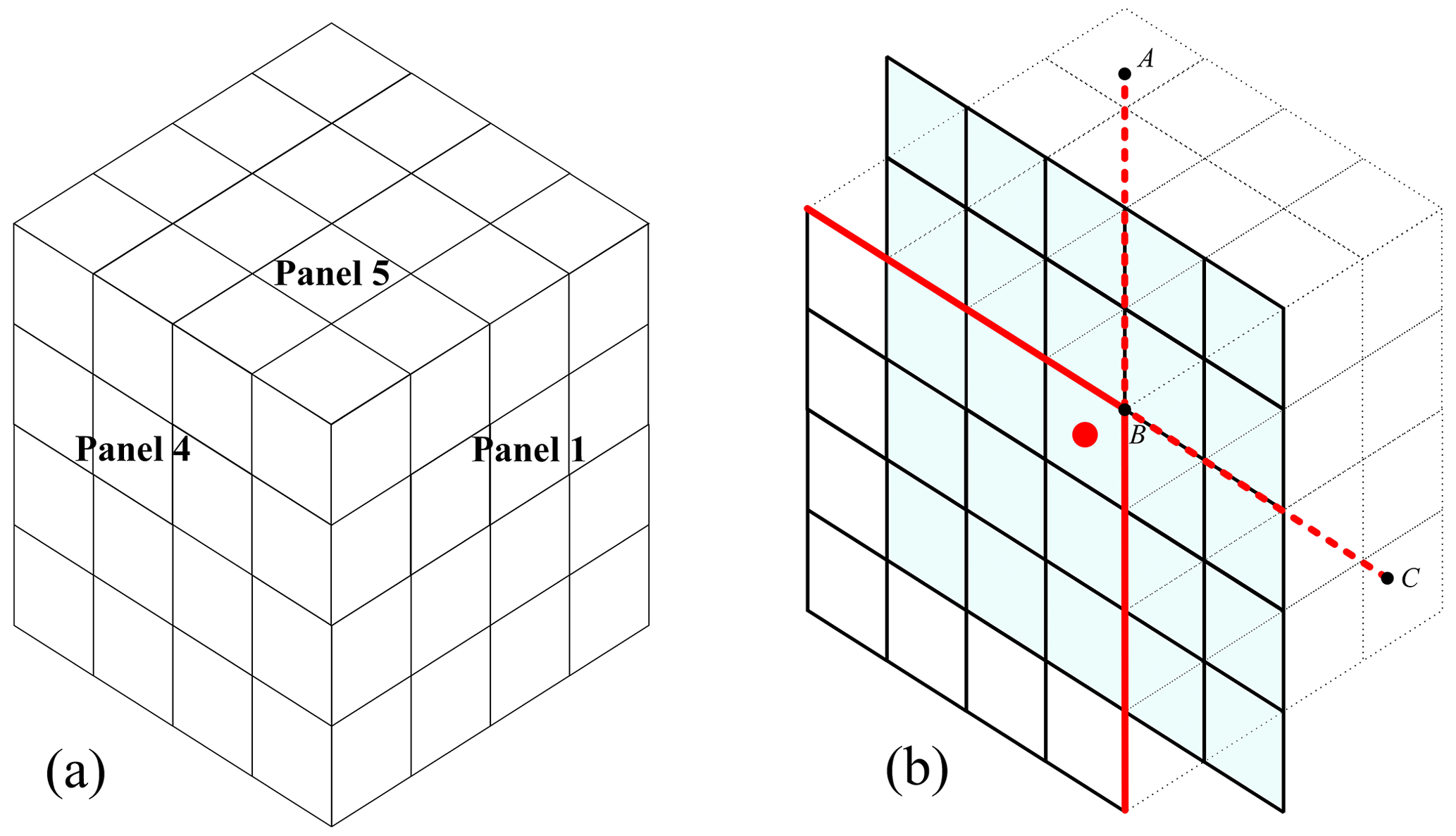
Figure 2 (a) Adjacent area of panels 1, 4 and 5. (b) 5×5 reconstruction stencil nearby panel corner is represented by shade. The cell contains red dot is the target cell on panel 4; the magenta points are overlapped GQPs shared by panel 1 and panel 5; red solid lines are boundary of panel 4, red dash lines are extension line of panel 4 boundary line. A and C are points on dash line, B is the upper right corner point of panel 4.

3 Numerical discretization

The finite volume method computes the temporal tendency of cell-averaged quantities by evaluating the net flux across cell interfaces. The interfacial flux is obtained through Gaussian quadrature, where the field values at quadrature points are reconstructed spatially and then processed by a Riemann solver to determine the flux magnitude.

In this section, we present two distinct spatial reconstruction approaches: (1) a two-dimensional tensor product polynomial (TPP) method, and (2) a two-dimensional weighted essentially non-oscillatory (WENO2D) scheme based on tensor product polynomials. Each reconstruction yields two potential values at every Gaussian quadrature point (GQP). These values are then resolved into a single flux value using the Low Mach number Approximate Riemann Solver (LMARS) (Chen et al., 2013) or AUSM+-up (Liou, 2006; Ullrich et al., 2010). Even with an approximate Riemann solver like LMARS, the scheme preserves high-order because it combines high-order reconstructions from both sides of the cell interface to determine the flux. Finally, the total flux across each cell edge is computed by applying linear Gaussian quadrature integration along the interface.

According to the finite volume scheme, average Eq. (15) on cell i, j, we have

$$\begin{array}{}\text{(17)}& {\displaystyle }& {\displaystyle \frac{\partial {\stackrel{\mathrm{‾}}{\mathit{q}}}_{i,j}}{\partial t}}+{\displaystyle \frac{{\stackrel{\mathrm{‾}}{\mathit{F}}}_{i+\frac{\mathrm{1}}{\mathrm{2}},j}-{\stackrel{\mathrm{‾}}{\mathit{F}}}_{i-\frac{\mathrm{1}}{\mathrm{2}},j}}{\mathrm{\Delta }x}}+{\displaystyle \frac{{\stackrel{\mathrm{‾}}{\mathit{G}}}_{i,j+\frac{\mathrm{1}}{\mathrm{2}}}-{\stackrel{\mathrm{‾}}{\mathit{G}}}_{i,j-\frac{\mathrm{1}}{\mathrm{2}}}}{\mathrm{\Delta }y}}={\stackrel{\mathrm{‾}}{\mathit{S}}}_{i,j}\text{(18)}& {\displaystyle }& {\displaystyle \frac{\partial {\stackrel{\mathrm{‾}}{\mathit{q}}}_{i,j}}{\partial t}}={\displaystyle \frac{\mathrm{1}}{\mathrm{\Delta }x\mathrm{\Delta }y}}{\displaystyle \frac{\partial }{\partial t}}\underset{{\mathrm{\Omega }}_{i,j}}{\iint }\mathit{q}\mathrm{d}x\mathrm{d}y,{\stackrel{\mathrm{‾}}{\mathit{S}}}_{i,j}={\displaystyle \frac{\mathrm{1}}{\mathrm{\Delta }x\mathrm{\Delta }y}}\underset{{\mathrm{\Omega }}_{i,j}}{\iint }S\mathrm{d}x\mathrm{d}y\text{(19)}& {\displaystyle }& {\displaystyle }{\stackrel{\mathrm{‾}}{\mathit{F}}}_{i-\frac{\mathrm{1}}{\mathrm{2}},j}={\displaystyle \frac{\mathrm{1}}{\mathrm{\Delta }y}}\underset{e_{i-\frac{\mathrm{1}}{\mathrm{2}}}}{\int }\mathit{F}\mathrm{d}y,{\stackrel{\mathrm{‾}}{\mathit{F}}}_{i+\frac{\mathrm{1}}{\mathrm{2}},j}={\displaystyle \frac{\mathrm{1}}{\mathrm{\Delta }y}}\underset{e_{i+\frac{\mathrm{1}}{\mathrm{2}}}}{\int }\mathit{F}\mathit{d}y\text{(20)}& {\displaystyle }& {\displaystyle }{\stackrel{\mathrm{‾}}{\mathit{G}}}_{i,j-\frac{\mathrm{1}}{\mathrm{2}}}={\displaystyle \frac{\mathrm{1}}{\mathrm{\Delta }x}}\underset{e_{j-\frac{\mathrm{1}}{\mathrm{2}}}}{\int }\mathit{G}\mathrm{d}x,{\stackrel{\mathrm{‾}}{\mathit{G}}}_{i,j+\frac{\mathrm{1}}{\mathrm{2}}}={\displaystyle \frac{\mathrm{1}}{\mathrm{\Delta }x}}\underset{e_{j+\frac{\mathrm{1}}{\mathrm{2}}}}{\int }\mathit{G}\mathrm{d}x\end{array}$$

where Ω_i,j represents the region overlapped by cell (i, j), e_i−½, e_i+½, e_j−½, e_j+½ are left, right, bottom, top edges of cell (i, j).

The physical interpretation of equation Eq. (17) is that the average tendency of prognostic field q within cell (i, j) is governed by the average net flux and average source. In this study, we calculate these averages using Gaussian quadrature, the function points within each cell are illustrated in Fig. 3, the EQPs are share by adjacent cells, and CQPs are exclusive for each cell.

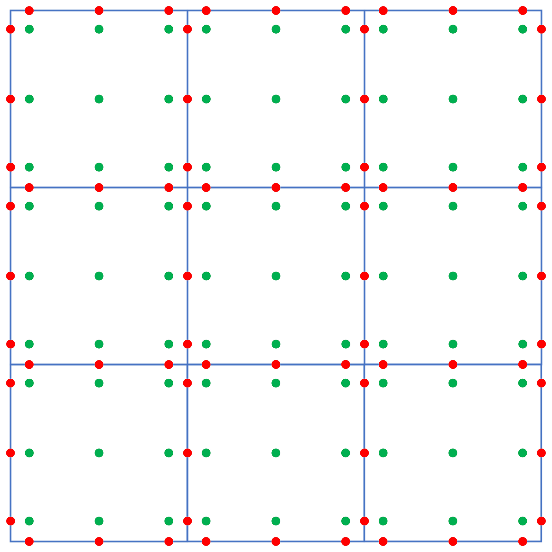
Figure 3 Function points on cell. Red points are edge quadrature points (EQP) or called flux points, green points are inner cell quadrature points (CQP).

Average on edge by 1D scheme:

$$\begin{array}{}\text{(21)}& {\stackrel{\mathrm{‾}}{\mathit{F}}}_{i+\frac{\mathrm{1}}{\mathrm{2}},j}\approx \sum _{\mathit{\xi }=\mathrm{1}}^{m_{\mathrm{e}}}{w}_{\mathit{\xi }}{\mathit{F}}_{\mathit{\xi }}=\mathit{w}\overrightarrow{\mathit{F}}\end{array}$$

where m_e is the number of quadrature points on each edge, $\mathit{w}=(w_{\mathrm{1}},w_{\mathrm{2}},\mathrm{\dots },w_{m_{\mathrm{e}}})$ is the 1D Gaussian quadrature coefficient vector. $\overrightarrow{\mathit{F}}=({\mathit{F}}_{\mathrm{1}},{\mathit{F}}_{\mathrm{2}},\mathrm{\dots },{\mathit{F}}_{m_{\mathrm{e}}}{)}^T$ is the vector of flux, the elements of $\overrightarrow{\mathit{F}}$ represent the flux on EQPs.

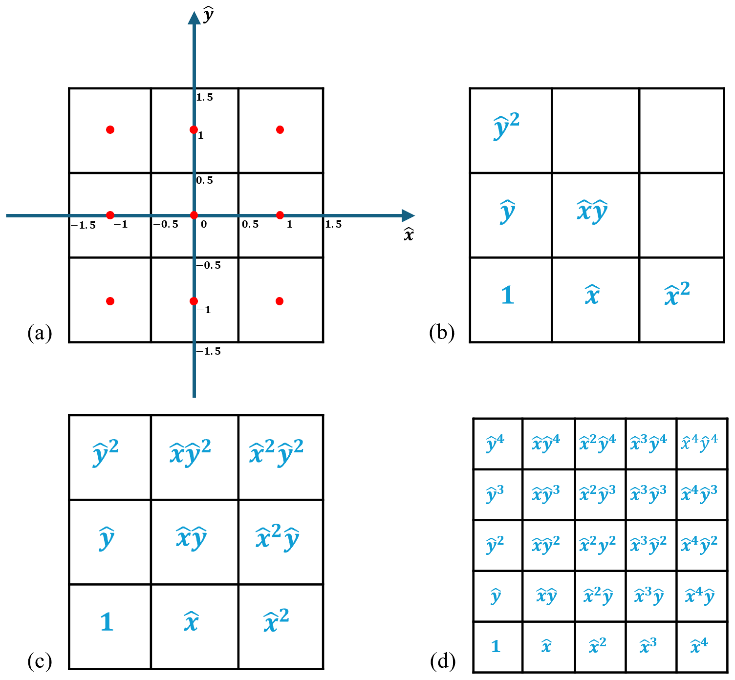
Figure 4 Reconstruction coordinate and polynomial terms on stencils. (a) Local reconstruction coordinate (the red points denote cell centers); (b) 2nd degree polynomial stencil; (c) TPP3 stencil; (d) TPP5 stencil.

Average in cell by 2D scheme:

$$\begin{array}{}\text{(22)}& {\stackrel{\mathrm{‾}}{\mathit{S}}}_{i,j}\approx \sum _{\mathit{\xi }=\mathrm{1}}^{m_{\mathrm{c}}}{W}_{\mathit{\xi }}{\mathit{S}}_{\mathit{\xi }}=\mathit{W}\overrightarrow{\mathit{S}}\end{array}$$

where m_c is the number of quadrature points on each cell, $\mathit{W}=(W_{\mathrm{1}},W_{\mathrm{2}},\mathrm{\dots },W_{m_{\mathrm{c}}})$ is the 2D Gaussian quadrature coefficient matrix, $\overrightarrow{\mathit{S}}=({\mathbf{S}}_{\mathrm{1}},{\mathit{S}}_{\mathrm{2}},\mathrm{\dots },{\mathbf{S}}_{m_{\mathrm{c}}}{)}^T$ is the vector of source term, the elements of S represent the source value on GQPs, superscript T stands for transpose matrix.

HOPE employs an equiangular cubed-sphere grid, where each panel undergoes uniform angular discretization into n_c×n_c cells. In the computational space (equiangular coordinates), each cell spans an angular interval of $\frac{\mathit{\pi }}{\mathrm{2}{n}_{\mathrm{c}}}$, therefore

$$\begin{array}{}\text{(23)}& \mathrm{\Delta }x=\mathrm{\Delta }y={\displaystyle \frac{\mathit{\pi }}{\mathrm{2}{n}_{\mathrm{c}}}}.\end{array}$$

This uniformity ensures that all cells are geometrically identical in the computational space, thereby avoiding the need for cell-specific treatment during reconstruction studies. In the following part of this section, we set a new computational space for reconstruction process. The local coordinate system ($\widehat{x}$, $\widehat{y}$) is established such that within each reconstruction stencil, the origin (0, 0) is located at the stencil center, the central cell spans [−0.5, 0.5] in both $\widehat{x}$ and $\widehat{y}$ directions, as shown in Fig. 4a. All of the cells have the same size in $\widehat{x}$, $\widehat{y}$ directions:

$$\begin{array}{}\text{(24)}& \mathrm{\Delta }\widehat{x}=\mathrm{\Delta }\widehat{y}=\mathrm{1}.\end{array}$$

On the cubed-sphere grid, a fixed reconstruction scheme yields consistent stencils across all cells. This structural homogeneity renders the reconstruction operation computationally equivalent to two-dimensional convolution, thereby enabling efficient GPU acceleration through PyTorch's built-in conv2d function.

3.1 Tensor product polynomial (TPP) reconstruction

HOPE employs genuinely two-dimensional reconstruction, simultaneously incorporating information in both spatial dimensions to minimize dimensional splitting errors. For computational efficiency, reconstruction algorithms using square stencils are computationally equivalent to convolution operations. This equivalence allows efficient implementation via PyTorch's conv2d function for acceleration.

To construct genuinely 2D reconstructions, the functional form of the reconstruction basis must be selected. A bivariate polynomial of degree d contains $\frac{(d+\mathrm{1})(d+\mathrm{2})}{\mathrm{2}}$ terms. As illustrated in Fig. 4b, the 6 terms of a bivariate quadratic polynomial (d=2) are insufficient to cover a square stencil. To address this, we adopt Tensor Product Polynomials (TPP) as basis functions. We denote a TPP function containing n×n terms as TPPn. Determining the coefficients of TPPn requires information from a n×n block of cells. When using a TPP reconstruction stencil of size n×n, HOPE achieves fifth-order accuracy when simulating smooth flow fields. We therefore designate a TPP reconstruction stencil of size n×n as an nth order TPP stencil, the 3rd and 5th order TPP stencils are shown in Fig. 4c and d.

A TPPn polynomial is expressed as

$$\begin{array}{}\text{(25)}& p\left(\widehat{x},\widehat{y}\right)=\sum _{\widehat{j}=\mathrm{1}}^n\sum _{\widehat{i}=\mathrm{1}}^n{a}_k{\widehat{x}}^{\widehat{i}-\mathrm{1}}{\widehat{y}}^{\widehat{j}-\mathrm{1}}=\sum _{k=\mathrm{1}}^N{a}_k{c}_k\left(\widehat{x},\widehat{y}\right)\end{array}$$

where n is width of stencil. a_k is the coefficient of each term, the term index $k=\widehat{i}+n(\widehat{j}-\mathrm{1})$, and $c_k(\widehat{x},\widehat{y})={\widehat{x}}^{\mathit{\alpha }}{\widehat{y}}^{\mathit{\beta }}$, $\mathit{\alpha }=k-\mathrm{int}\left(\frac{k-\mathrm{1}}{n}\right)n-\mathrm{1}$, $\mathit{\beta }=\mathrm{int}\left(\frac{k-\mathrm{1}}{n}\right)$, “int” is equivalent to Fortran's intrinsic function int( ) that truncates to integer values. N=n² is the cell number in stencil and also the term number of the TPP. We define column vectors $\mathit{c}(\widehat{x},\widehat{y})=\mathit{\left\{}{c}_k\right(\widehat{x},\widehat{y})\mathrm{|}k=\mathrm{1},\mathrm{2},\mathrm{3},\mathrm{\dots },N\mathit{\}}$ and $\mathit{a}=\mathit{\{}{a}_k\mathrm{|}k=\mathrm{1},\mathrm{2},\mathrm{3},\mathrm{\dots },N\mathit{\}}$, the point value on ($\widehat{x}$, $\widehat{y}$) can be written as

$$\begin{array}{}\text{(26)}& p\left(\widehat{x},\widehat{y}\right)=\mathit{c}\left(\widehat{x},\widehat{y}\right)\cdot \mathit{a}.\end{array}$$

The volume integration average (VIA) of prognostic field q on cell Ω_i,j is represented by

$$\begin{array}{}\text{(27)}& {\stackrel{\mathrm{‾}}{q}}_{i,j}={\displaystyle \frac{\mathrm{1}}{\mathrm{\Delta }{\widehat{x}}_{i,j}\mathrm{\Delta }{\widehat{y}}_{i,j}}}\int \underset{{\mathrm{\Omega }}_{i,j}}{\int }p\left(\widehat{x},\widehat{y}\right)\mathrm{d}\widehat{x}\mathrm{d}\widehat{y}.\end{array}$$

$\mathrm{\Delta }{\widehat{x}}_{i,j}$, $\mathrm{\Delta }{\widehat{y}}_{i,j}$ are length of edges $\widehat{x}$, $\widehat{y}$ of cell Ω_i,j in computational space. The VIA value ${\stackrel{\mathrm{‾}}{\mathit{q}}}_i$ on each cell is predicted by time integration, we wish to determine the coefficient vector a by these VIA values. HOPE employs an equiangular cubed-sphere grid, wherein each cell in computational space can be considered a perfectly identical square, according to Eq. (24), we may assume without loss of generality that $\mathrm{\Delta }{\widehat{x}}_{i,j}=\mathrm{\Delta }{\widehat{y}}_{i,j}=\mathrm{1}$, and Eq. (27) becomes

$$\begin{array}{}\text{(28)}& {\stackrel{\mathrm{‾}}{q}}_{i,j}=\int \underset{{\mathrm{\Omega }}_{i,j}}{\int }p\left(\widehat{x},\widehat{y}\right)\mathrm{d}\widehat{x}\mathrm{d}\widehat{y}=\int \underset{{\mathrm{\Omega }}_{i,j}}{\int }\mathit{c}\cdot \mathit{a}\mathrm{d}\widehat{x}\mathrm{d}\widehat{y}={\mathit{\psi }}_{i,j}\cdot \mathit{a}\end{array}$$

where

$${\mathit{\psi }}_{i,j}=\int \underset{{\mathrm{\Omega }}_{i,j}}{\int }\mathit{c}\mathrm{d}\widehat{x}\mathrm{d}\widehat{y}=\left(\begin{array}{l}\int \underset{{\mathrm{\Omega }}_{i,j}}{\int }{c}_{\mathrm{1}}\mathrm{d}\widehat{x}\mathrm{d}\widehat{y}\\ \int \underset{{\mathrm{\Omega }}_{i,j}}{\int }{c}_{\mathrm{2}}\mathrm{d}\widehat{x}\mathrm{d}\widehat{y}\\ \mathrm{⋮}\\ \int \underset{{\mathrm{\Omega }}_{i,j}}{\int }{c}_N\mathrm{d}\widehat{x}\mathrm{d}\widehat{y}\end{array}\right),$$

combining N cells. We have following linear system

$$\begin{array}{}\text{(29)}& {\displaystyle }& {\displaystyle }\mathbf{A}\mathit{a}=\stackrel{\mathrm{‾}}{\mathit{q}}\text{(30)}& {\displaystyle }& {\displaystyle }\mathbf{A}=\left(\begin{array}{l}{\mathit{\psi }}_{\mathrm{1}}^T\\ {\mathit{\psi }}_{\mathrm{2}}^T\\ \mathrm{⋮}\\ {\mathit{\psi }}_N^T\end{array}\right),\stackrel{\mathrm{‾}}{\mathit{q}}=\left(\begin{array}{l}{\stackrel{\mathrm{‾}}{\mathit{q}}}_{\mathrm{1}}\\ {\stackrel{\mathrm{‾}}{\mathit{q}}}_{\mathrm{2}}\\ \mathrm{⋮}\\ {\stackrel{\mathrm{‾}}{\mathit{q}}}_N\end{array}\right)\end{array}$$

and polynomial coefficient a can be obtain by solving Eq. (29).

$$\begin{array}{}\text{(31)}& \mathit{a}={\mathbf{A}}^{-\mathrm{1}}\stackrel{\mathrm{‾}}{\mathit{q}}\end{array}$$

The reconstruction values on M points can be obtained by following formula

$$\begin{array}{}\text{(32)}& \mathit{p}=\mathbf{C}\mathit{a}={\mathbf{CA}}^{-\mathrm{1}}\stackrel{\mathrm{‾}}{\mathit{q}}=\mathbf{R}\stackrel{\mathrm{‾}}{\mathit{q}}\end{array}$$

where $\mathit{p}=\left(\begin{array}{l}p\left({\widehat{x}}_{\mathrm{1}},{\widehat{y}}_{\mathrm{1}}\right)\\ p\left({\widehat{x}}_{\mathrm{2}},{\widehat{y}}_{\mathrm{2}}\right)\\ \mathrm{⋮}\\ p\left({\widehat{x}}_M,{\widehat{y}}_M\right)\end{array}\right),\mathbf{C}=\left(\begin{array}{l}{\mathit{c}}_{\mathrm{1}}^T\\ {\mathit{c}}_{\mathrm{2}}^T\\ \mathrm{⋮}\\ {\mathit{c}}_M^T\end{array}\right)$, ${\mathit{c}}_m^T={\mathit{c}}^T({\widehat{x}}_m,{\widehat{y}}_m)$, $m=\mathrm{1},\mathrm{2},\mathrm{\dots },M$, superscript T stands for transpose matrix, (${\widehat{x}}_m$, ${\widehat{y}}_m$) represents the mth function point on target cell. The reconstruction matrix

$$\begin{array}{}\text{(33)}& \mathbf{R}={\mathbf{CA}}^{-\mathrm{1}}.\end{array}$$

In practical implementation, the reconstruction matrix R needs to be computed only once during model initialization and stored in memory. Crucially, a fundamental advantage of our cubed-sphere grid dynamical core implementation lies in employing a globally shared reconstruction matrix R. This unification signifies that a single instance of R applies identically to all grid cells, thereby significantly reducing memory/VRAM requirements, and enabling straightforward utilization of PyTorch's conv2d for accelerated reconstruction. For example, the TPP reconstruction procedure can be directly formulated as a two-dimensional convolutional operation using R as the convolution kernel.

3.2 Genuine two-dimensional WENO

Weighted Essentially Non-Oscillatory (WENO) represents an adaptive algorithm that dynamically preserves high-order approximation accuracy in smooth flow regions while automatically degenerating to robust low-order reconstruction near discontinuities for effective shock capturing. Shi et al. (2002) mentioned two different approaches for constructing a fifth-order finite volume WENO scheme: the “Genuine 2D” method and the “Dimension by Dimension” method.

For HOPE, within the Genuine 2D framework, nth order accuracy WENO scheme employs a n×n master stencil partitioned into $\frac{(n+\mathrm{1}{)}^{\mathrm{2}}}{\mathrm{4}}$ distinct $\frac{(n+\mathrm{1})}{\mathrm{2}}\times \frac{(n+\mathrm{1})}{\mathrm{2}}$ sub-stencils, for example:

• a.

  WENO3: third-order reconstruction utilizes a 3×3 cell stencil that decomposes into four 2×2 sub-stencils.

• b.

  WENO5: fifth-order accuracy employs a 5×5 master stencil partitioned into nine distinct 3×3 sub-stencils (complete schematic representations of these decomposition strategies are provided in Figs. 5 and 6).

The scheme's theoretical order of accuracy fundamentally depends on the proper determination of optimal linear weights for the multidimensional stencil combination. These weights, when correctly derived, enable the weighted superposition of sub-stencils to recover full high-order accuracy in smooth solution regions. While Shi et al. (2002) indicated the theoretical possibility of computing these weights through Lagrange interpolation basis analysis, they omitted specific implementation details. In this section, we present the methods for constructing genuine two-dimensional WENO (WENO 2D) schemes using least squares method.

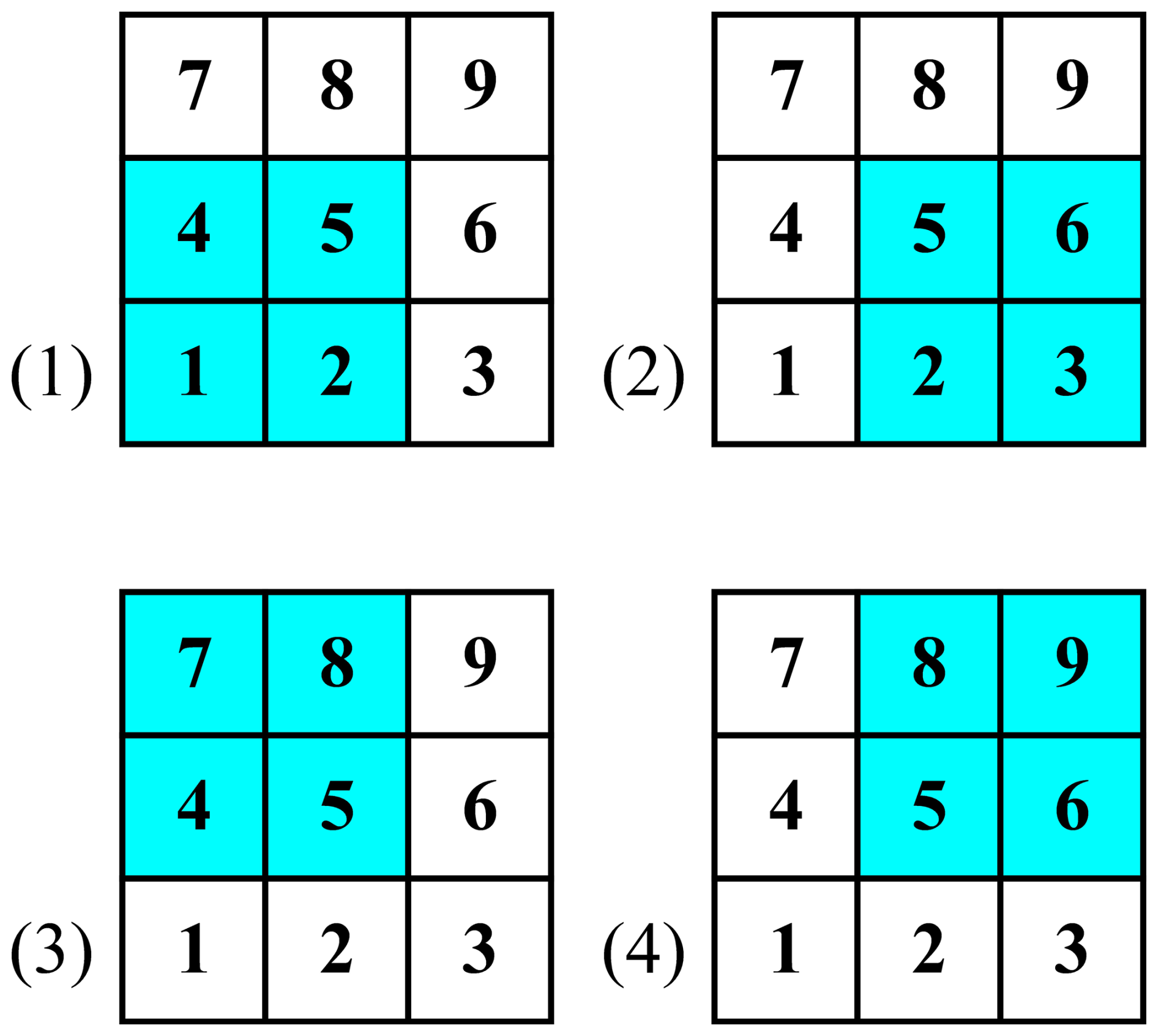
Figure 5 Stencils of 3rd order WENO 2D. The high order stencil contains cells No. 1–9, blue ones represent the cells in sub-stencils (1)–(4).

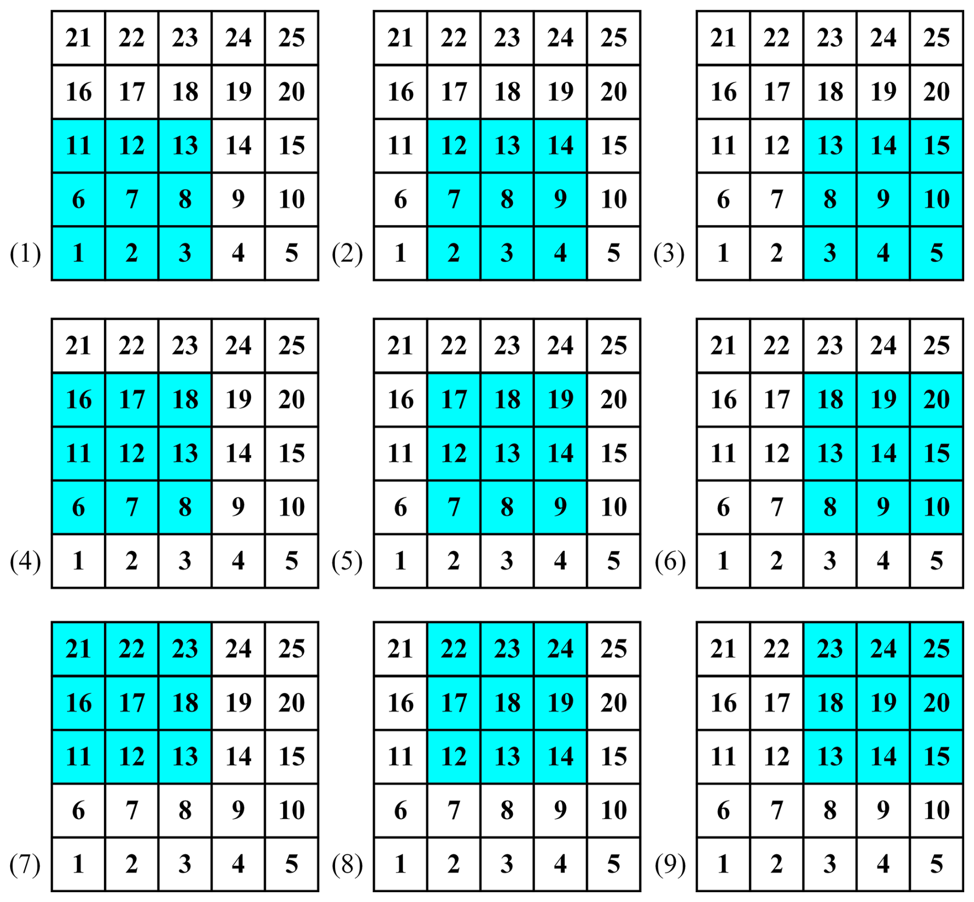
Figure 6 Stencils of 5th order WENO 2D. The high order stencil contains cells No. 1–25, blue ones represent the cells in sub-stencils (1)–(9).

We construct WENO 2D based on TPP and square stencil. As mentioned in previous section, a nth order stencil contains N=n² cells, and the full stencil (also called high-order stencil) width is h=n. Decomposing the high-order stencil into $s={\left(\frac{n+\mathrm{1}}{\mathrm{2}}\right)}^{\mathrm{2}}$ sub-stencils, there are s_c=s cells in each sub-stencil (also called low-order stencil), and the sub-stencil width is $l=\frac{n+\mathrm{1}}{\mathrm{2}}$. We define p_H as the high- order reconstruction polynomial, and p_i represents ith sub-stencil reconstruction polynomial, they share the same expression as Eq. (25) with different stencil width and coefficient a. For the reconstruction point ($\widehat{x}$, $\widehat{y}$), suppose $p_{\mathrm{H}}(\widehat{x},\widehat{y})$ is the reconstruction value of high-order stencil, the reconstruction values of sub-stencils are stored in vector $\mathit{p}=\left(p_{\mathrm{1}}\right(\widehat{x},\widehat{y}),p_{\mathrm{2}}(\widehat{x},\widehat{y}),\mathrm{\cdots },p_{\mathrm{s}}(\widehat{x},\widehat{y}){)}^T$. The intention of constructing the optimal linear weights is to determine the unique weights $\mathit{\gamma }=({\mathit{\gamma }}_{\mathrm{1}},{\mathit{\gamma }}_{\mathrm{2}},\mathrm{\cdots },{\mathit{\gamma }}_{\mathrm{s}})$, such that

$$\begin{array}{}\text{(34)}& p_{\mathrm{H}}={\mathbf{R}}_{\mathrm{H}}\stackrel{\mathrm{‾}}{\mathit{q}}=\mathit{\gamma }\cdot \mathit{p}\end{array}$$

where the elements of vector $\stackrel{\mathrm{‾}}{\mathit{q}}=(q_{\mathrm{1}},q_{\mathrm{2}},\mathrm{\cdots },q_N{)}^T$ represent VIA of each cell in high-order stencil. ${\mathbf{R}}_{\mathrm{H}}=\left(r_{H_j}\right)$, $j=\mathrm{1},\mathrm{2},\mathrm{\dots },N$ is the reconstruction matrix of high-order stencil.

It should be noted that Eq. (34) appears overdetermined at first glance. However, subsequent analysis demonstrates that the solution obtained via the least squares method satisfies Eq. (34) exactly. Specifically, in the case of square stencils, the rank of the system defined by Eq. (34) becomes s, resulting in a unique solution for the linear system. This finding aligns with observations presented in Hu and Shu (1999) regarding their research on Triangular Meshes.

The computation of γ requires the integration of both high-order and low-order reconstruction matrices into a unified linear system. For each sub-stencil i we define the reconstruction matrix R_i=(r_ik), $k=\mathrm{1},\mathrm{2},\mathrm{\dots },s_{\mathrm{c}}$ (computed via Eq. 33). and ${\mathbf{R}}_{{\mathrm{L}}_i}=\left(r_{{\mathrm{L}}_{ij}}\right)$, $j=\mathrm{1},\mathrm{2},\mathrm{\dots },N$ is the extension matrix of R_i. The matrix relationship is expressed as

$$\begin{array}{}\text{(35)}& {\left({\mathbf{R}}_i\right)}_{\mathrm{1}\times s_{\mathrm{c}}}(\mathbf{E}{)}_{s_{\mathrm{c}}\times N}={\left({\mathbf{R}}_{{\mathrm{L}}_i}\right)}_{\mathrm{1}\times N}\end{array}$$

where the subscripts denote matrix dimensions. The correspondence matrix E=(e_ij), $i=\mathrm{1},\mathrm{2},\mathrm{\dots },s_{\mathrm{c}}$; $j=\mathrm{1},\mathrm{2},\mathrm{\dots },N$ encodes the cell relationships between stencils: when the ith cell in low-order stencil is the same as the jth cell in high order stencil, e_ij=1, otherwise, e_ij=0.

Substitute Eq. (32) into Eq. (34), yield

$$\begin{array}{}\text{(36)}& {\mathbf{R}}_{\mathrm{H}}\stackrel{\mathrm{‾}}{q}=\sum _{i=\mathrm{1}}^s{\mathbf{R}}_{{\mathrm{L}}_i}{\mathit{\gamma }}_i\stackrel{\mathrm{‾}}{q}.\end{array}$$

We set ${\mathbf{R}}_{\mathrm{L}}=({\mathbf{R}}_{{\mathrm{L}}_{\mathrm{1}}},{\mathbf{R}}_{{\mathrm{L}}_{\mathrm{2}}},\mathrm{\dots },{\mathbf{R}}_{{\mathrm{L}}_{\mathrm{s}}}{)}^T$, Eq. (36) becomes

$$\begin{array}{}\text{(37)}& {\mathbf{R}}_{\mathrm{L}}\mathit{\gamma }={\mathbf{R}}_{\mathrm{H}}.\end{array}$$

The unknown optimal weights vector γ can be determined by following least square procedure

$$\begin{array}{}\text{(38)}& \mathit{\gamma }={\left({\mathbf{R}}_{\mathrm{L}}^T{\mathbf{R}}_{\mathrm{L}}\right)}^{-\mathrm{1}}{\mathbf{R}}_{\mathrm{L}}^T{\mathbf{R}}_{\mathrm{H}}.\end{array}$$

However, the elements of γ could be negative, which would cause unstable. A split technique mentioned by Shi et al. (2002) was adopted to solve this problem. The optimal weights can be split into two parts:

$$\begin{array}{}\text{(39)}& {\stackrel{\mathrm{̃}}{\mathit{\gamma }}}^{+}={\displaystyle \frac{\mathit{\theta }\left|\mathit{\gamma }\right|+\mathit{\gamma }}{\mathrm{2}}},{\stackrel{\mathrm{̃}}{\mathit{\gamma }}}^{-}={\mathit{\gamma }}^{+}-\mathit{\gamma }\end{array}$$

where the constant θ=3. For keeping the sum of weights to 1, ${\stackrel{\mathrm{̃}}{\mathit{\gamma }}}^{\pm }$ and new value of γ^± can be rescaled as:

$$\begin{array}{}\text{(40)}& {\mathit{\sigma }}^{\pm }=\sum _{i=\mathrm{1}}^s{\stackrel{\mathrm{̃}}{\mathit{\gamma }}}_i^{\pm }\end{array}$$

and

$$\begin{array}{}\text{(41)}& {\mathit{\gamma }}_i^{\pm }={\displaystyle \frac{{\stackrel{\mathrm{̃}}{\mathit{\gamma }}}_i^{\pm }}{{\mathit{\sigma }}^{\pm }}}i=\mathrm{1},\mathrm{2},\mathrm{\dots },s\end{array}$$

where ${\stackrel{\mathrm{̃}}{\mathit{\gamma }}}_i^{\pm }$ is the ith element of ${\stackrel{\mathrm{̃}}{\mathit{\gamma }}}^{\pm }$, ${\mathit{\gamma }}_i^{\pm }$ is the ith element of γ^±.

The WENO scheme adaptively assigns nonlinear weights ω_i, ($i=\mathrm{1},\mathrm{2},\mathrm{\dots },s$) to each candidate stencil to suppress unphysical oscillations during high-order reconstruction. Essentially, it gives greater weight to stencils identified as smooth over the local cell, while suppressing the influence of those containing discontinuities by assigning them smaller weights. Several nonlinear weighting schemes have been developed to meet these criteria, including WENO-JS (Jiang and Shu, 1996), WENO-Z (Borges et al., 2008), WENO-Z+ (Acker et al., 2016), WENO-Z+M (Luo and Wu, 2021), among others.

In this work, we employ the WENO-Z formulation as our baseline scheme. While most existing WENO schemes were originally developed for one-dimensional problems, we propose a two-dimensional extension of WENO-Z through modification of τ, a crucial coefficient that governs the scheme's higher-order accuracy properties.

For stencil i the nonlinear weight is given as

$$\begin{array}{}\text{(42)}& {\displaystyle }& {\displaystyle }{\mathit{\omega }}_i^{\pm }={\displaystyle \frac{{\mathit{\alpha }}_i^{\pm }}{\sum _{i=\mathrm{1}}^s{\mathit{\alpha }}_i^{\pm }}}\text{(43)}& {\displaystyle }& {\displaystyle }{\mathit{\alpha }}_i^{\pm }={\mathit{\gamma }}_i^{\pm }\left[\mathrm{1}+{\left({\displaystyle \frac{\mathit{\tau }}{{\mathit{\beta }}_i+\mathit{\epsilon }}}\right)}^{\mathrm{2}}\right]\text{(44)}& {\displaystyle }& {\displaystyle }\mathit{\tau }={\displaystyle \frac{\mathrm{2}}{(s-\mathrm{1})s}}\sum _{\mathit{\eta }=\mathrm{1}}^{s-\mathrm{1}}\sum _{\mathit{\psi }=\mathit{\eta }+\mathrm{1}}^s\left|{\mathit{\beta }}_{\mathit{\psi }}-{\mathit{\beta }}_{\mathit{\eta }}\right|\end{array}$$

where $\mathit{\epsilon }={\mathrm{10}}^{-\mathrm{14}}$ is introduced to prevent division by zero. The smooth indicators β_i quantify the smoothness of reconstruction functions within the target cell. We employ a formulation analogous to that described in Zhu and Shu (2019).

As mentioned in Eq. (24), all cells participating in reconstruction within HOPE's computational space can be treated as identical unit squares with $\mathrm{\Delta }\widehat{x}=\mathrm{\Delta }\widehat{y}=\mathrm{1}$. Thus, the smooth indicator for sub-stencil i is expressed as:

$$\begin{array}{}\text{(45)}& {\mathit{\beta }}_i=\sum _{\mathit{\zeta }=\mathrm{1}}^l\int \underset{\mathrm{\Omega }}{\int }{\left[{\displaystyle \frac{{\partial }^{\mathit{\zeta }}}{\partial {\widehat{x}}^{{\mathit{\zeta }}_{\mathrm{1}}}\partial {\widehat{y}}^{{\mathit{\zeta }}_{\mathrm{2}}}}}{p}_i\left(\widehat{x},\widehat{y}\right)\right]}^{\mathrm{2}}\mathrm{d}\widehat{x}\mathrm{d}\widehat{y}\end{array}$$

where ${\mathit{\zeta }}_{\mathrm{1}}+{\mathit{\zeta }}_{\mathrm{2}}=\mathit{\zeta }$ and ζ>0, ζ₁, ${\mathit{\zeta }}_{\mathrm{2}}\in [\mathrm{0},n]$, and l is the sub-stencil width.

The reconstruction value on point ($\widehat{x}$, $\widehat{y}$) is expressed by:

$$\begin{array}{}\text{(46)}& q\left(\widehat{x},\widehat{y}\right)=\sum _{i=\mathrm{1}}^s\left({\mathit{\sigma }}^{+}{\mathit{\omega }}_i^{+}-{\mathit{\sigma }}^{-}{\mathit{\omega }}_i^{-}\right)p_i\left(\widehat{x},\widehat{y}\right).\end{array}$$

3.3 Treatment of the panel boundaries

The cubed sphere grid comprises 12 panel boundaries, and the flux across the interface between any two panels must be computed at the quadrature points situated on the edges of the boundary cells, as depicted in Fig. 7a. However, a challenge arises because the coordinates across these panel boundaries are discontinuous. Given that the TPP reconstruction necessitates a square stencil, the values of the cells outside the domain (referred to as ghost cells) must be computed through interpolation within the adjacent panel, as illustrated in Fig. 7b. While Ullrich et al. (2010) proposed a one-sided interpolation scheme, our testing with the HOPE model revealed that using a similar one-sided ghost cell interpolation approach around panel boundaries resulted in instability when scheme exceeded 7th order of accuracy. To address this limitation, we redesigned the ghost cell interpolation scheme to incorporate information from both panels adjacent to the boundary. This modified approach ensures stable integration even for very high-order schemes, as validated in tests up to 13th-order accuracy.

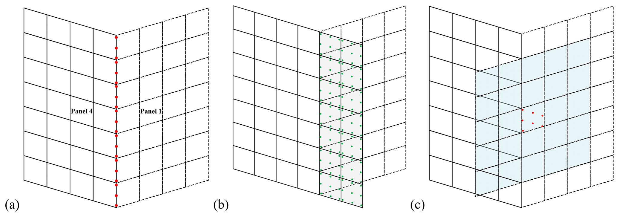
Figure 7 Points and cells close to panel boundary. (a) Flux points (red points) on the interface between Panel 1 and Panel 4, the flux across each panel at these points are determined by Riemann solver, which merges the reconstruction outcomes from both panels into a single flux value; (b) ghost cells (shaded cells) out of Panel 4 boundary, with green points representing the GQPs in these cells; (c) cells requirement for 5th order ghost cell interpolation stencil, red points represent the GQPs located in the ghost cell on Panel 4, the blue shaded region represents the TPP reconstruction stencil (on Panel 1) to interpolate these red GQPs.

3.3.1 Ghost cell interpolation

To achieve arbitrary high-order accuracy, we propose a ghost cell interpolation scheme that incorporates information from both sides of the panel boundary. Since the ghost cell values are inherently unknown prior to interpolation, our approach involves an initial estimation through an iterative process. Specifically, the method iteratively performs ghost cell interpolation until the increments of the cell values converge to within a specified tolerance.

Through mathematical analysis (detailed in the Appendix), we demonstrate that this iterative process can be expressed as a linear mapping, thereby eliminating the need for actual iterations. However, direct computation of the mapping matrix requires inversion of a large matrix, which poses significant computational and memory challenges. To address this, we implement the iterative interpolation process using PyTorch and leverage its automatic differentiation capability to efficiently obtain the interpolation matrix.

The complete methodology, as derived in the Appendix, proceeds as follows:

1. Initialization: all ghost cell values are initialized to zero (denoted as g⁽⁰⁾=0, where the superscript indicates the iteration number).

2. Interpolation: the Gaussian quadrature points (GQPs) in the ghost cells are interpolated using the Tensor Product Polynomial (TPP) stencil. For instance, considering two adjacent panels (Fig. 7a), any out-domain cell in Panel 4 (shaded cell in Fig. 7b) contains GQPs that physically reside in Panel 1. These GQPs are interpolated using the TPP stencil shown in Fig. 7c, which incorporates relevant ghost cells from Panel 1.

3. Update and convergence check: after interpolating all GQPs, the ghost cell values are updated via Gaussian quadrature (Eq. 22), yielding g⁽¹⁾. The L₂-norm residual $r^{\left(k\right)}={∥{\mathit{g}}^{(k+\mathrm{1})}-{\mathit{g}}^{\left(k\right)}∥}_{\mathrm{2}}$ is then computed. Steps 2–3 repeat until r^(k)<ϵ, where $\mathit{ϵ}=\mathrm{1}\times {\mathrm{10}}^{-\mathrm{14}}$ for double precision and $\mathit{ϵ}=\mathrm{1}\times {\mathrm{10}}^{-\mathrm{5}}$ for single precision. In practice, convergence typically occurs within 10 iterations, so we fix the iteration count at 10 for consistency.

This process establishes a linear mapping $\mathcal{G}:\mathit{q}\to \mathit{g}$ from known cell values to ghost cell values. As proven in Eq (A12), the mapping's linearity implies that $\mathcal{G}=\frac{\partial \mathit{g}}{\partial \mathit{q}}$ forms a matrix, which we efficiently compute using PyTorch's autograd functionality. This approach avoids explicit matrix inversion while maintaining numerical precision.

It is important to note that overlapping GQPs occur at the corner positions of the cubed-sphere grid, as illustrated by the magenta points in Fig. 2b. These points lie on the interface shared by adjacent panels (e.g., Panel 1 and Panel 5). Consequently, during ghost value interpolation, two distinct interpolated values are obtained at these overlapping points – one from each adjoining panel. The final interpolated value is computed as the average of these two values. Since the interpolation performed on each individual panel is high-order, the approximation order is preserved when taking this average.

𝒢 is a sparse matrix containing many zero entries. To avoid unnecessary memory costs, we adopt the Compressed Sparse Row (CSR) format for storing 𝒢. Furthermore, the size of 𝒢 is extremely large-making direct application of “torch.autograd.functional.jacobian” to generate 𝒢 computationally infeasible. Our implementation for generating ghost cell interpolation matrix achieves significant acceleration and substantially reduces VRAM demand compared to PyTorch's native “torch.autograd.functional.jacobian” function. The key optimizations are:

1. Parallel Multi-Row Computation: utilizing “torch.vmap” to encapsulate “torch.func.vjp”, enabling simultaneous computation of multiple matrix rows.

2. CSR Compression and Incremental Disk Storage:

   • a.

     Employing Compressed Sparse Row (CSR) format for matrix representation.

   • b.

     Implementing incremental disk storage, where computed data batches are immediately written to disk after processing, avoiding prolonged VRAM retention.

3. Tunable Batch Processing: adjusting the number of rows processed per iteration maximizes GPU utilization while respecting VRAM constraints (e.g., 24 GB on NVIDIA RTX 3090).

It should be note that the model grid does not change during simulation, the ghost interpolation matrix  𝒢 needs to be calculated only once in initialization progress.

3.3.2 Fields conversion between panels

Due to the differing coordinate systems across panels, field variables must be appropriately transformed when transferring information between adjacent panels. To illustrate this process, we consider the interface between Panel 1 and Panel 4, as depicted in Figs. 2a and 7a. Although flux points are shared between the two panels, their coordinate representations are discontinuous across the interface.

To ensure consistency, two key transformations are required:

1. Metric reset for mass variables: the mass-related prognostic quantities must be recomputed in the target panel's coordinate system to maintain metric consistency.

2. Wind vector transformation: velocity components (or other vector quantities) must be converted from the source panel's local coordinate frame to that of the target panel.

This coordinate conversion ensures proper continuity and physical consistency when interpolating or exchanging data across panel boundaries.

Suppose ${\mathit{q}}_{\mathrm{1}}=\left[\right(\sqrt{G}\mathit{\varphi }{)}_{\mathrm{1}},(\sqrt{G}\mathit{\varphi }u{)}_{\mathrm{1}},(\sqrt{G}\mathit{\varphi }v{)}_{\mathrm{1}}{]}^T$ and ${\mathit{q}}_{\mathrm{4}}=\left[\right(\sqrt{G}\mathit{\varphi }{)}_{\mathrm{4}},(\sqrt{G}\mathit{\varphi }u{)}_{\mathrm{4}},(\sqrt{G}\mathit{\varphi }v{)}_{\mathrm{4}}{]}^T$ represent the fields on panel 1 and 4. The mass field conversion from panel 4 to panel 1 is expressed by

$$\begin{array}{}\text{(47)}& (\sqrt{G}\mathit{\varphi }{)}_{\mathrm{4}}^{\mathrm{1}}={\displaystyle \frac{{\sqrt{G}}_{\mathrm{4}}}{{\sqrt{G}}_{\mathrm{1}}}}(\sqrt{G}\mathit{\varphi }{)}_{\mathrm{1}}\end{array}$$

the subscript represents the target panel and the superscript stands for source panel.

The transformation of momentum vectors between panels is performed in two sequential steps to maintain proper tensor consistency. The contravariant momentum components in Panel 1 are first projected onto the global spherical coordinate system using the transformation matrix J, as defined in Eq. (10). The resulting spherical momentum components are then transformed into the contravariant representation specific to Panel 4, ensuring compatibility with the target panel's local coordinate system.

$$\begin{array}{}\text{(48)}& {\displaystyle }& {\displaystyle }\left[\begin{array}{c}{\left(\sqrt{G}\mathit{\varphi }{u}_{\mathrm{s}}\right)}_{\mathrm{1}}\\ {\left(\sqrt{G}\mathit{\varphi }{v}_{\mathrm{s}}\right)}_{\mathrm{1}}\end{array}\right]={\mathbf{J}}_{\mathrm{1}}\left[\begin{array}{c}(\sqrt{G}\mathit{\varphi }u{)}_{\mathrm{1}}\\ (\sqrt{G}\mathit{\varphi }v{)}_{\mathrm{1}}\end{array}\right]\text{(49)}& {\displaystyle }& {\displaystyle }\left[\begin{array}{c}(\sqrt{G}\mathit{\varphi }u{)}_{\mathrm{4}}\\ (\sqrt{G}\mathit{\varphi }v{)}_{\mathrm{4}}\end{array}\right]={\mathbf{J}}_{\mathrm{4}}^{-\mathrm{1}}{\displaystyle \frac{{\sqrt{G}}_{\mathrm{4}}}{{\sqrt{G}}_{\mathrm{1}}}}\left[\begin{array}{c}{\left(\sqrt{G}\mathit{\varphi }{u}_{\mathrm{s}}\right)}_{\mathrm{1}}\\ {\left(\sqrt{G}\mathit{\varphi }{v}_{\mathrm{s}}\right)}_{\mathrm{1}}\end{array}\right]\end{array}$$

where J₁ is the J matrix on panel 1, ${\mathbf{J}}_{\mathrm{4}}^{-\mathrm{1}}$ is the inverse matrix of J on panel 4. (u_s, v_s) are zonal wind and meridional wind, (u, v) are contravariant wind components. Since the vector conversion is linear process, Eqs. (48) and (49) can be merged into following equation

$$\begin{array}{}\text{(50)}& \left[\begin{array}{c}(\sqrt{G}\mathit{\varphi }u{)}_{\mathrm{4}}\\ (\sqrt{G}\mathit{\varphi }v{)}_{\mathrm{4}}\end{array}\right]={\mathbf{C}}_{\mathrm{1},\mathrm{4}}\left[\begin{array}{c}(\sqrt{G}\mathit{\varphi }u{)}_{\mathrm{1}}\\ (\sqrt{G}\mathit{\varphi }v{)}_{\mathrm{1}}\end{array}\right]\end{array}$$

where matrix ${\mathbf{C}}_{\mathrm{1},\mathrm{4}}=\frac{{\sqrt{G}}_{\mathrm{4}}}{{\sqrt{G}}_{\mathrm{1}}}{\mathbf{J}}_{\mathrm{4}}^{-\mathrm{1}}{\mathbf{J}}_{\mathrm{1}}$, the subscript stands for converting vector form panel 1 to panel 4.

The mass and vector are also need to be converted on GQPs in the same manner.

3.4 Riemann solver

Following spatial reconstruction, discontinuous solutions arise on either side of each flux point location. Since the majority of atmospheric flow speeds correspond to small Mach numbers, we adopt the Low Mach number Approximate Riemann Solver (Chen et al., 2013) and AUSM⁺-up (Liou, 2006; Ullrich et al., 2010) as Riemann solvers to determine the flux at the edge quadrature points (EQPs).

3.4.1 Low Mach number approximate Riemann solver (LMARS)

Spatial reconstruction gives the left and right state vector,

$$\begin{array}{}\text{(51)}& {\mathit{q}}_{\mathrm{L}}=\left[\begin{array}{l}(\sqrt{G}\mathit{\varphi }{)}_{\mathrm{L}}\\ (\sqrt{G}\mathit{\varphi }u{)}_{\mathrm{L}}\\ (\sqrt{G}\mathit{\varphi }v{)}_{\mathrm{L}}\end{array}\right],{\mathit{q}}_{\mathrm{R}}=\left[\begin{array}{l}(\sqrt{G}\mathit{\varphi }{)}_{\mathrm{R}}\\ (\sqrt{G}\mathit{\varphi }u{)}_{\mathrm{R}}\\ (\sqrt{G}\mathit{\varphi }v{)}_{\mathrm{R}}\end{array}\right].\end{array}$$

First of all, we convert the contravariant wind u to physical speed u^⊥ that is perpendicular to the cell edge.

$$\begin{array}{}\text{(52)}& u^{\perp }={\displaystyle \frac{u}{{\sqrt{G}}^{ii}}},i=\left\{\begin{array}{cc}\mathrm{1},& x\mathrm{direction}\\ \mathrm{2},& y\mathrm{direction}\end{array}\right.\end{array}$$

For example, in x direction, $u^{\perp }=\frac{u}{{\sqrt{G}}^{\mathrm{11}}}$, and there is no summation over i in Eq. (52).

The wind speed m^* and geopotential ϕ are calculated by

$$\begin{array}{}\text{(53)}& {\displaystyle }& {\displaystyle }{m}^{*}={\displaystyle \frac{\mathrm{1}}{\mathrm{2}}}\left(u_{\mathrm{L}}^{\perp }+u_{\mathrm{R}}^{\perp }-{\displaystyle \frac{{\mathit{\varphi }}_{\mathrm{R}}-{\mathit{\varphi }}_{\mathrm{L}}}{c}}\right)\text{(54)}& {\displaystyle }& {\displaystyle }\mathit{\varphi }={\displaystyle \frac{\mathrm{1}}{\mathrm{2}}}\left[{\mathit{\varphi }}_{\mathrm{L}}+{\mathit{\varphi }}_{\mathrm{R}}-c\left(u_{\mathrm{R}}^{\perp }-u_{\mathrm{L}}^{\perp }\right)\right]\text{(55)}& {\displaystyle }& {\displaystyle }c={\displaystyle \frac{c_{\mathrm{L}}+c_{\mathrm{R}}}{\mathrm{2}}}\text{(56)}& {\displaystyle }& {\displaystyle }{c}_{\mathrm{L}}={\sqrt{\mathit{\varphi }}}_{\mathrm{L}},c_{\mathrm{R}}={\sqrt{\mathit{\varphi }}}_{\mathrm{R}}.\end{array}$$

c is the phase speed of external gravity wave, the subscript “L”, “R” represent the left and right side of cell edge.

Once m^* is determined, we convert it back to contravariant speed by

$$\begin{array}{}\text{(57)}& m=m^{*}{\sqrt{G}}^{ii}.\end{array}$$

We define the pressure-driven flux as

$$\begin{array}{}\text{(58)}& P={\displaystyle \frac{\mathrm{1}}{\mathrm{2}}}\sqrt{G}{\mathit{\varphi }}_t^{\mathrm{2}}.\end{array}$$

The flux across the cell edge is then given by

$$\begin{array}{}\text{(59)}& {\displaystyle }& {\displaystyle }\mathit{F}={\displaystyle \frac{\mathrm{1}}{\mathrm{2}}}m\left[\left({\mathit{q}}_{\mathrm{L}}+{\mathit{q}}_{\mathrm{R}}\right)-\mathrm{sign}\left(m\right)\left({\mathit{q}}_{\mathrm{R}}-{\mathit{q}}_{\mathrm{L}}\right)\right]+\mathit{P}\text{(60)}& {\displaystyle }& {\displaystyle }\mathit{P}=\left(\begin{array}{l}\mathrm{0}\\ G^{\mathrm{1}i}P\\ G^{\mathrm{2}i}P\end{array}\right),i=\left\{\begin{array}{cc}\mathrm{1},& x\mathrm{direction}\\ \mathrm{2},& y\mathrm{direction}\end{array}\right..\end{array}$$

For calculation of G (the flux in y direction) the method is similar.

3.4.2 Advection upstream splitting method for all speeds (AUSM⁺-up)

The differences between AUSM⁺-up and LMARS lie in the method of determining the wind speed m^* and pressure-driven flux P. In AUSM⁺-up

$$\begin{array}{}\text{(61)}& m^{*}=cM\end{array}$$

where c denotes the gravity phase speed defined in Eq. (55). Mach number M is expressed as

$$\begin{array}{}\text{(62)}& \begin{array}{rl}M=& M_{\left(\mathrm{4}\right)}^{+}\left(M_{\mathrm{L}}\right)+M_{\left(\mathrm{4}\right)}^{-}\left(M_{\mathrm{R}}\right)-K_p\max \left(\mathrm{1}-\mathit{\sigma }{\stackrel{\mathrm{‾}}{M}}^{\mathrm{2}},\mathrm{0}\right)\\ & {\displaystyle \frac{P_{\mathrm{R}}-P_{\mathrm{L}}}{c^{\mathrm{2}}\mathit{\varphi }}}\end{array}\end{array}$$

where $M_{\mathrm{L}}=\frac{u_L^{\perp }}{c}$, $M_{\mathrm{R}}=\frac{u_R^{\perp }}{c}$, ${\stackrel{\mathrm{‾}}{M}}^{\mathrm{2}}=\frac{(u_{\mathrm{L}}^{\perp }{)}^{\mathrm{2}}+(u_{\mathrm{R}}^{\perp }{)}^{\mathrm{2}}}{\mathrm{2}{c}^{\mathrm{2}}}$, and

$$\begin{array}{}\text{(63)}& {\displaystyle }& {\displaystyle }{M}_{\left(\mathrm{4}\right)}^{\pm }\left(M\right)=\left\{\begin{array}{ll}\frac{\mathrm{1}}{\mathrm{2}}(M\pm \left|M\right|),& \left|M\right|\ge \mathrm{1}\\ M_{\left(\mathrm{2}\right)}^{\pm }\left(M\right)\left[\mathrm{1}\mp \mathrm{16}\mathit{\beta }{M}_{\left(\mathrm{2}\right)}^{\mp }\left(M\right)\right],& \left|M\right|<\mathrm{1}\end{array}\right.\text{(64)}& {\displaystyle }& {\displaystyle }{M}_{\left(\mathrm{2}\right)}^{\pm }\left(M\right)=\pm {\displaystyle \frac{\mathrm{1}}{\mathrm{4}}}(M\pm \mathrm{1}{)}^{\mathrm{2}}.\end{array}$$

The pressure-driven flux is expressed as

$$\begin{array}{}\text{(65)}& \begin{array}{rl}P=& P_{\left(\mathrm{5}\right)}^{+}\left(M_{\mathrm{L}}\right)P_{\mathrm{L}}+P_{\left(\mathrm{5}\right)}^{-}\left(M_{\mathrm{R}}\right)P_{\mathrm{R}}+-\mathrm{2}{K}_u{P}_{\left(\mathrm{5}\right)}^{+}\left(M_{\mathrm{L}}\right)\\ & P_{\left(\mathrm{5}\right)}^{-}\left(M_{\mathrm{R}}\right)\mathit{\varphi }c\left(u_{\mathrm{R}}^{\perp }-u_{\mathrm{L}}^{\perp }\right)\end{array}\end{array}$$

where $P_{\mathrm{L}}=\frac{\mathrm{1}}{\mathrm{2}}{\mathit{\varphi }}_{\mathrm{L}}^{\mathrm{2}}$, $P_{\mathrm{R}}=\frac{\mathrm{1}}{\mathrm{2}}{\mathit{\varphi }}_{\mathrm{R}}^{\mathrm{2}}$, and

$$\begin{array}{}\text{(66)}& \begin{array}{rl}& P_{\left(\mathrm{5}\right)}^{\pm }=\\ & \left\{\begin{array}{ll}\frac{\mathrm{1}}{\mathrm{2}}(\mathrm{1}\pm \mathrm{sign}(M\left)\right),& \left|M\right|\ge \mathrm{1}\\ M_{\left(\mathrm{2}\right)}^{\pm }\left(M\right)\left[(\pm \mathrm{2}-M)\mp \mathrm{16}\mathit{\alpha }M{M}_{\left(\mathrm{2}\right)}^{\mp }\left(M\right)\right],& \left|M\right|<\mathrm{1}\end{array}\right.\end{array}\end{array}$$

The mathematical meaning of sign(M) (returning −1, 0, or 1 based on the sign of M) is standard. The coefficients take the values: σ=1, $\mathit{\alpha }=\frac{\mathrm{3}}{\mathrm{16}}$, $\mathit{\beta }=\frac{\mathrm{1}}{\mathrm{8}}$, $K_p=\frac{\mathrm{1}}{\mathrm{4}}$, $K_u=\frac{\mathrm{3}}{\mathrm{4}}$.

Once m^* and P are computed, the flux across the cell edge can be calculated using Eqs. (57) to (60).

3.5 Temporal integration

We use the explicit Runge–Kutta (RK) as time marching scheme, Wicker and Skamarock (2002) described a 3rd order RK with three stages (achieves third-order accuracy exclusively when applied to linear problems). For the prognostic fields q, the integration step from time slot n to n+1:

$$\begin{array}{}\text{(67)}& {\displaystyle }& {\displaystyle }{\mathit{q}}^{*}={\mathit{q}}^n+{\displaystyle \frac{\mathrm{\Delta }t}{\mathrm{3}}}\left({\displaystyle \frac{\partial {\mathit{q}}^n}{\partial t}}\right)\text{(68)}& {\displaystyle }& {\displaystyle }{\mathit{q}}^{**}={\mathit{q}}^{*}+{\displaystyle \frac{\mathrm{\Delta }t}{\mathrm{2}}}\left({\displaystyle \frac{\partial {\mathit{q}}^{*}}{\partial t}}\right)\text{(69)}& {\displaystyle }& {\displaystyle }{\mathit{q}}^{n+\mathrm{1}}={\mathit{q}}^n+\mathrm{\Delta }t\left({\displaystyle \frac{\partial {\mathit{q}}^{**}}{\partial t}}\right)\end{array}$$

where Δt is the time step, and temporal tendency terms $\frac{\partial \mathbf{q}}{\partial t}$ can be obtain by Eqs. (15) and (16). In our numerical experiments, the choice of different time marching schemes influenced only the integration stability; it had no significant impact on the simulation norm errors, non-oscillatory property, or conservation property.

4 High performance implementation and automatic differentiation

The spatial operator and temporal integration of HOPE can be easily implemented using PyTorch. Specifically, the spatial reconstruction given by Eq. (32) is implemented as a convolution operation, while the Gaussian quadrature can be efficiently expressed as a matrix-vector multiplication. Leveraging PyTorch's highly optimized built-in functions for both convolution and quadrature operations ensures superior performance on GPUs.

Furthermore, PyTorch's role as a versatile AI development platform provides automatic differentiation capabilities across the entire computation graph. This streamlines implementation and enables efficient gradient computation for all components.

For the reconstruction implementation. Suppose the cubed sphere grid comprises n_c cells in x-direction within each panel, including ghost cells. The panel number is n_p, and the shallow water equation involves n_v prognostic variables per cell, we write the cell state tensor q with the shape (n_v, n_p, 1, n_c, n_c). The TPP reconstruction weight tensor R has shape (n_poc, 1, s_w, s_w), where n_poc is the number of points required to be interpolated within each cell (including EQP and CQP), s_w denotes the stencil width (same as the stencil width represented by n in Sec. 3.1). The reconstruction can be executed by a simple command (pseudo-code):

$$\begin{array}{}\text{(70)}& \begin{array}{rl}{\mathit{q}}_{\mathrm{rec}}=& \mathrm{torch}.\mathrm{nn}.\mathrm{functional}.\mathrm{conv}\mathrm{2}\mathrm{d}\left(\mathit{q}\cdot \mathrm{view}\left(n_{\mathrm{v}}{n}_{\mathrm{p}},\mathrm{1},n_{\mathrm{c}},n_{\mathrm{c}}\right),\right.\\ & \left.\mathbf{R}\right)\mathrm{view}\left(n_{\mathrm{v}},n_{\mathrm{p}},n_{\mathrm{poc}},n_{\mathrm{c}},n_{\mathrm{c}}\right)\end{array}\end{array}$$

where the shape of q_rec is (n_v, n_p, n_poc, n_c, n_c).

We exclusively demonstrate the flux computation procedure at cell edges as an illustrative example, where Gaussian quadrature is employed to obtain edge-averaged fluxes. The analogous procedure applies to source term integration at CQPs. The edge state tensor q_e, corresponding to the EQPs along each cell edge, is subsequently expressed as:

$$\begin{array}{}\text{(71)}& {\mathit{q}}_{\mathrm{e}}={\mathit{q}}_{\mathrm{rec}}(\mathrm{\dots },\mathrm{pes}:\mathrm{pee},:,:)\end{array}$$

where subscript “e” represents edges on cell including L(left), R(right), B(bottom), T(top). “pes, pee” are start and end point indices on edge e. The shape of q_e (including q_L, q_R, q_B, q_T) is (n_v, n_p, n_poe, n_c, n_c). n_poe denotes the number of edge quadrature points (EQPs). This value is computed as $n_{\mathrm{poe}}=\mathrm{pee}-\mathrm{pes}$ in PyTorch implementations, whereas in Fortran it is calculated as $n_{\mathrm{poe}}=\mathrm{pee}-\mathrm{pes}+\mathrm{1}$, reflecting the difference in array indexing conventions between the two languages.

After spatial reconstruction, the resulting data is utilized in the Riemann solver for EQPs and for source term computation on CQPs.  Subsequently, integration is performed on both EQPs and CQPs to calculate the net flux and the cell-averaged source term tendency. The cell-edge flux tensor F with dimensions (n_v, n_p, n_poe, n_c, n_c) is obtained after the Riemann solver.

There is a dimensionality mismatch between the flux tensor and weight tensor during using matrix multiplication. For the Gaussian quadrature implementation, consider an edge Gaussian quadrature weight tensor g_e with shape (n_poe), if an edge flux tensor $\stackrel{\mathrm{̃}}{\mathit{F}}$ has shape (n_v, n_p, n_c, n_c, n_poe), the Gaussian quadrature can be expressed by:

$$\begin{array}{}\text{(72)}& {\mathit{F}}_g=\mathrm{torch}.\mathrm{matmul}\left(\stackrel{\mathrm{̃}}{\mathit{F}},{\mathbf{g}}_{\mathrm{e}}\right)\end{array}$$

where the shape of ${\mathit{F}}_g(n_{\mathrm{v}},n_{\mathrm{p}},n_{\mathrm{c}},n_{\mathrm{c}})$ is the average flux on edge. In this operation, n_poe must occupy the last dimension of $\stackrel{\mathrm{̃}}{\mathit{F}}$, to permit “torch.matmul” execution. We note, however, that in the flux tensor F obtained from the Riemann solver, n_poe corresponds to the third dimension, direct matrix multiplication is therefore not feasible.

To address this dimensionality issue, two methods are available. The first method involves rearranging the n_poc dimension to the last position using the “torch.tensor.permute” operation in PyTorch, this allows Gaussian integrations to be naturally implemented through the “torch.matmul” operation. The second method, which avoids the need for the “permute” operation, maintains the original dimension sequence. Instead, Gaussian integrations are performed using the “torch.einsum” function. This function sums the product of the elements of the input arrays along dimensions specified using a notation based on the Einstein summation convention.

$$\begin{array}{}\text{(73)}& {\mathit{F}}_g=\mathrm{torch}.\mathrm{einsum}\left({}^{\prime }vnpij,p\to vni{j}^{\prime },\mathit{F},{\mathbf{g}}_{\mathrm{e}}\right)\end{array}$$

We have conducted performance tests comparing the two methods, and the results indicate that the second method is approximately 5% faster than the first. Specifically, the first method took 649 seconds, while the second method took 616 s. The test was set as a one-day steady state geostrophic flow (with details provided in Sect. 5.2) simulation at a resolution of C900 ($\mathrm{\Delta }x=\mathrm{\Delta }y=\mathrm{0.1}$°), using 3rd order accuracy reconstruction stencil. The time step was 30 s, and the default data type used was “torch.float32” (single precision).

The Riemann solver implementation on flux points is way easier, only needs to call “torch.sign” for Eq. (59), while all other operations can be executed using basic arithmetic: addition, subtraction, multiplication, and division. During a Runge–Kutta sub-step, there are no dependencies, and neither “for” loops nor “if” statements are required in the HOPE kernel code. This algorithm fully leverages the capabilities of the GPU.

5 Numerical experiments

The HOPE dynamical core is evaluated using the standard test cases (Test 1, 2, 5, and 6) for the spherical shallow water model as described in Williamson et al. (1992), along with the perturbed jet flow case proposed by Galewsky et al. (2004). Additionally, a dam-break experiment is designed to demonstrate the HOPE model's capability in capturing shock waves.

In our experiments, the grid resolutions are denoted by the count of cells along one dimension on each panel of the cubed sphere; for instance, C90 signifies that each panel is subdivided into a 90×90 grid, corresponding to a grid interval of $\mathrm{\Delta }x=\mathrm{\Delta }y=\mathrm{1}$°.

We measure the conservation errors by defining the normalized error ϵ_r of the variable η as ${\mathit{ϵ}}_r=\frac{I_g\left({\mathit{\eta }}^n\right)-I_g\left({\mathit{\eta }}^{\mathrm{0}}\right)}{I_g\left({\mathit{\eta }}^{\mathrm{0}}\right)}$, where η⁰ and ηⁿ stand for η value at initial time and time slot n, respectively. The global integral is defined as:

$$\begin{array}{}\text{(74)}& I\left(\mathit{\eta }\right)=\sum _{p=\mathrm{1}}^{n_{\mathrm{p}}}\sum _{j=\mathrm{1}}^{n_{\mathrm{c}}}\sum _{i=\mathrm{1}}^{n_{\mathrm{c}}}{\sqrt{G}}_{i,j,p}{\mathit{\eta }}_{i,j,p}\end{array}$$

where ${\mathit{\eta }}_{i,j,p}$ represents the average value of η in cell (i, j, p).

We use three kinds of norm errors to measure the simulation errors,

$$\begin{array}{}\text{(75)}& {\displaystyle }& {\displaystyle }{L}_{\mathrm{1}}={\displaystyle \frac{I\left[\mathit{\varphi }(i,j,p)-{\mathit{\varphi }}_{\mathrm{ref}}(i,j,p)\right]}{I\left[{\mathit{\varphi }}_{\mathrm{ref}}(i,j,p)\right]}}\text{(76)}& {\displaystyle }& {\displaystyle }{L}_{\mathrm{2}}=\sqrt{{\displaystyle \frac{I\left[{\left(\mathit{\varphi }(i,j,p)-{\mathit{\varphi }}_{\mathrm{ref}}(i,j,p)\right)}^{\mathrm{2}}\right]}{I\left[{\mathit{\varphi }}_{\mathrm{ref}}^{\mathrm{2}}(x,y,p)\right]}}}\text{(77)}& {\displaystyle }& {\displaystyle }{L}_{\mathrm{\infty }}={\displaystyle \frac{\max \left|\mathit{\varphi }(i,j,p)-{\mathit{\varphi }}_{\mathrm{ref}}(i,j,p)\right|}{\max \left|{\mathit{\varphi }}_{\mathrm{ref}}(i,j,p)\right|}}\end{array}$$

the subscript “ref” represents reference state.

5.1 Cosine bell advection

The Solid Body Rotation Cosine Bell (Case 1 from Williamson et al., 1992) is commonly employed to assess noise generated by panel boundaries, as noted by Chen and Xiao (2008) and Ullrich et al. (2010). The wind field is given by

$$\begin{array}{}\text{(78)}& {\displaystyle }& {\displaystyle }{u}_{\mathrm{s}}=u_{\mathrm{0}}(\cos \mathit{\theta }\cos \mathit{\alpha }+\cos \mathit{\lambda }\sin \mathit{\theta }\sin \mathit{\alpha })\text{(79)}& {\displaystyle }& {\displaystyle }{v}_{\mathrm{s}}=-u_{\mathrm{0}}\sin \mathit{\lambda }\sin \mathit{\alpha }\end{array}$$

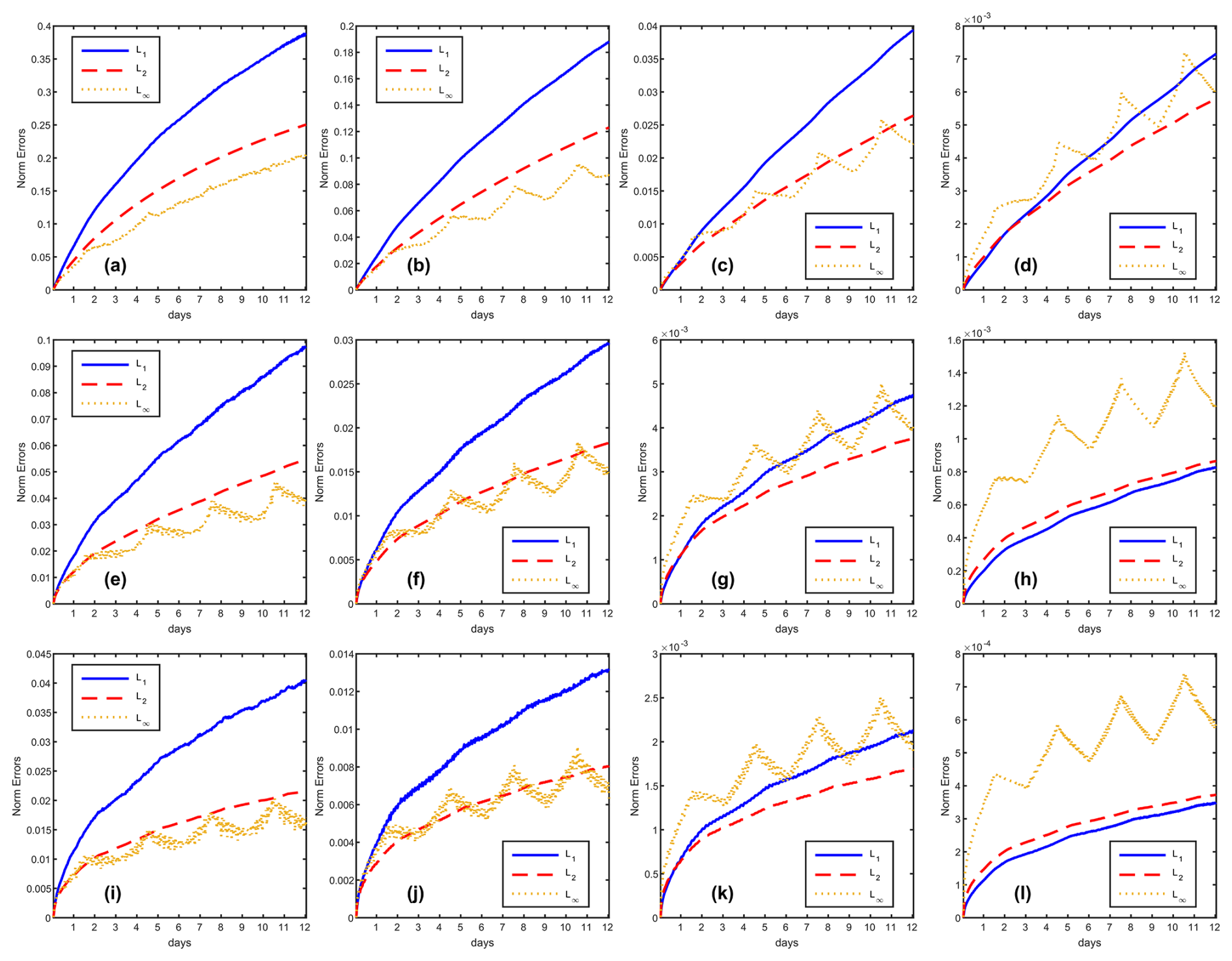
Figure 8 The variation of norm errors during simulation days for the cosine bell advection test case, with direction parameter α=0. The rows represent reconstruction schemes TPP3, TPP5 and TPP7, the columns stand for grid C30, C45, C90 and C180.

where u_s, v_s are zonal wind and meridional wind, earth radius is a=6 371 220 m, basic flow speed $u_{\mathrm{0}}=\frac{\mathrm{2}\mathit{\pi }a}{\mathrm{12}\cdot \mathrm{86}\mathrm{400}}$ m s⁻¹. The initial height is defined as

$$\begin{array}{}\text{(80)}& h(\mathit{\lambda },\mathit{\theta })=\left\{\begin{array}{ll}{h}_{\mathrm{0}}\left(\mathrm{1}+\cos \frac{\mathit{\pi }{d}_{\mathrm{s}}}{R}\right),& r<R\\ \mathrm{0},& r\ge R\end{array}\right.\end{array}$$

where λ, θ are longitude and latitude. The basic height h₀=1000 m. The great circle distance between (λ, θ) and the initial center point of cosine bell (λ_c, ${\mathit{\theta }}_{\mathrm{c}})=(\mathrm{3}\mathit{\pi }/\mathrm{2},\mathrm{0})$ is expressed by $d_{\mathrm{s}}=a\cdot \arccos [\sin {\mathit{\theta }}_{\mathrm{c}}\sin \mathit{\theta }+\cos {\mathit{\theta }}_{\mathrm{c}}\cos \mathit{\theta }\cos (\mathit{\lambda }-{\mathit{\lambda }}_{\mathrm{c}}\left)\right]$. The radius $R=a/\mathrm{3}$.

Figure 8 presents the norm errors for a 12 d simulation at α=0; results for $\mathit{\alpha }=\mathit{\pi }/\mathrm{2}$ are identical. The temporal evolution of L₁ and L₂ norm errors does not exhibit a pronounced signature attributable to panel boundaries. In contrast, the L_∞ norm error evolution shows significant sensitivity to panel boundaries, varying considerably with grid resolution and reconstruction order. When using low resolution and low reconstruction order (TPP3 with C30 grid), oscillations induced by panel boundaries are relatively weak. However, as the model resolution or reconstruction order increases, the influence of panel boundaries on the L_∞ norm error manifests as a distinct four-peak pattern, corresponding to the four longitudinally aligned panel boundaries of the cubed-sphere grid.

Figure 9 shows the 12 d simulation norm errors for $\mathit{\alpha }=\mathit{\pi }/\mathrm{4}$. In this test configuration, the cosine bell initially moves alone the interface between Panel 1 and Panel 5, and subsequently moves along the interface between Panel 3 and Panel 6. The temporal evolution of L₁ and L₂ norm errors display two gentle peaks, corresponding to the errors generated as the cosine bell crosses these panel interfaces. Similar to Fig. 8, the L_∞ norm error progressively exceeds the L₁ and L₂ norm errors as grid resolution and reconstruction order increase.

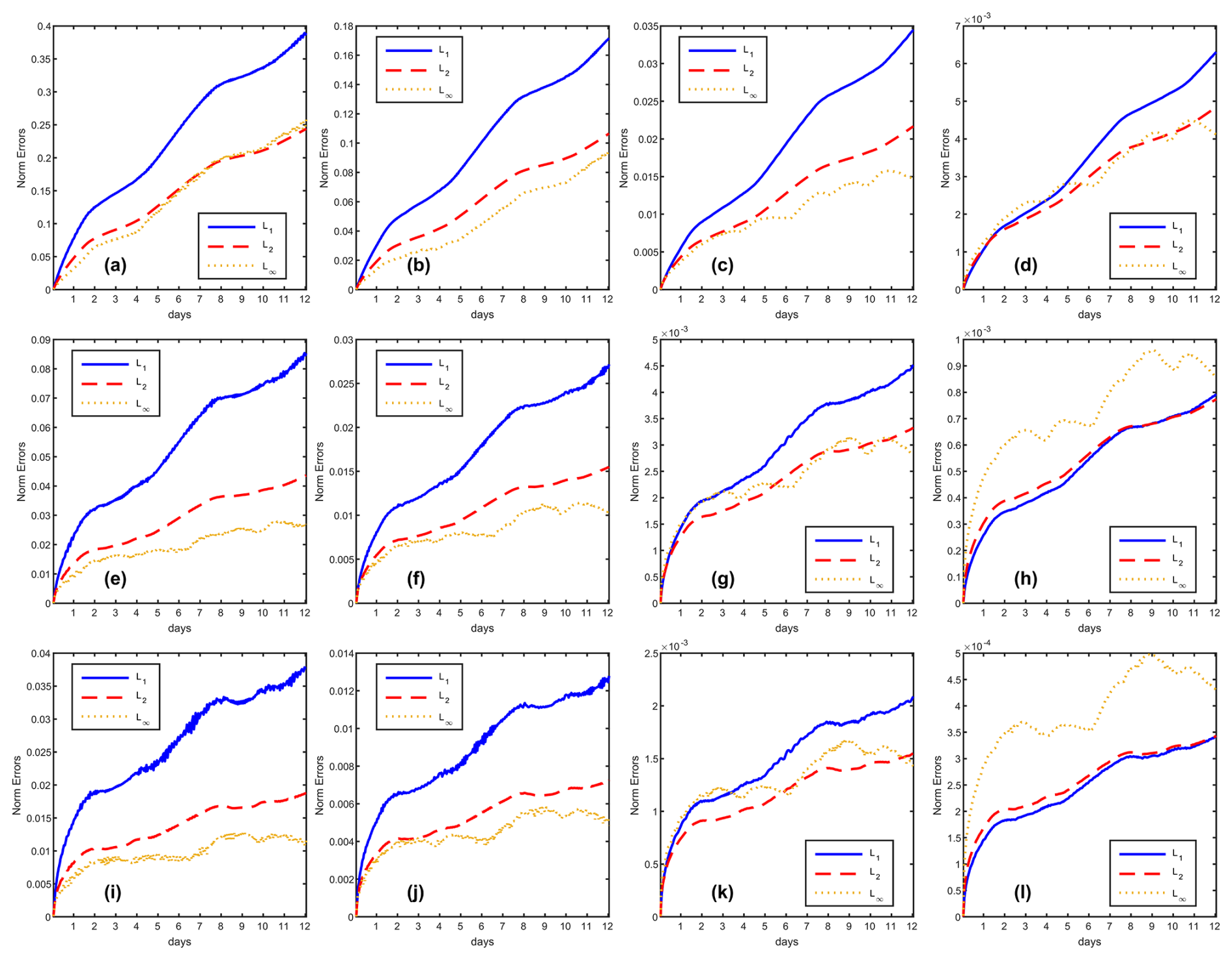
Figure 9 The variation of norm errors during simulation days for the cosine bell advection test case, with direction parameter $\mathit{\alpha }=\mathit{\pi }/\mathrm{4}$. The rows represent reconstruction schemes TPP3, TPP5 and TPP7, the columns stand for grid C30, C45, C90 and C180.

Because the Cosine Bell field lacks infinite continuity, the convergence rate of the norm errors cannot exceed second order in our tests, regardless of the reconstruction order employed. This observation aligns with the key point emphasized in our paper: high-order numerical methods achieve their design accuracy only when the flow field is sufficiently smooth. Discontinuities in the flow field violate the fundamental premise of polynomial reconstruction (as discontinuities impair the continuity of higher derivatives, leading to non-convergence of the Taylor series). This inherent sensitivity to smoothness is precisely the factor causing norm errors to be influenced by cubed-sphere panel boundaries. When using low-order reconstruction schemes at low resolutions, the Tensor Product Polynomial (TPP) reconstruction employs lower-degree polynomials and is consequently less sensitive to the smoothness of the flow field. Conversely, high-order TPP reconstruction requires the flow field to possess higher-order continuity to maintain accuracy; it is thus more sensitive to discontinuities. Insufficiently smooth flow fields can introduce numerical oscillations with high-order schemes. Therefore, while TPP5 and TPP7 yield lower L_∞ norm error magnitudes than TPP3, they exhibit more pronounced oscillations caused by the cubed-sphere panel boundaries.

5.2 Steady state geostrophic flow

Steady state geostrophic flow is the 2nd case in Williamson et al. (1992), it provided an analytical solution for spherical shallow water equations, it was widely used in accuracy test for shallow water models. The analytical solution is a steady state, which means the initial filed is the exact solution. The initial wind field replicates the formulation given in Eqs. (78) and (79), while the initial geopotential is expressed as

$$\begin{array}{}\text{(81)}& \mathit{\varphi }={\mathit{\varphi }}_{\mathrm{0}}-\left(a\mathrm{\Omega }{u}_{\mathrm{0}}+{\displaystyle \frac{u_{\mathrm{0}}^{\mathrm{2}}}{\mathrm{2}}}\right)(-\cos \mathit{\lambda }\cos \mathit{\theta }\sin \mathit{\alpha }+\sin \mathit{\theta }\cos \mathit{\alpha }{)}^{\mathrm{2}}\end{array}$$

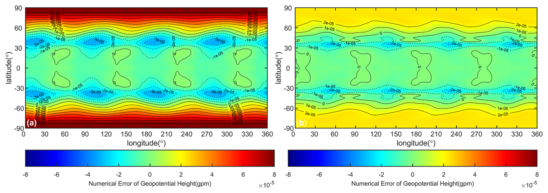
Figure 10 Numerical errors (simulation result minus exact solution) of geopotential for steady state flow with Riemann solvers (a) LMARS and (b) AUSM⁺-up. The reconstruction scheme is TPP5, and the model resolution is C90.

where $\mathrm{\Omega }=\mathrm{7.292}\times {\mathrm{10}}^{-\mathrm{5}}$ s⁻¹ is the earth rotation angular velocity, basic geopotential ϕ₀=29 400 m² s⁻², α=0 denotes the rotation angle transcribed between the physical north pole and the center of the northern panel on the cubed-sphere grid, and gravity acceleration g=9.80616 m s⁻². The conversion between the spherical wind (u_s, v_s) and contravariant wind is given by Eq. (9).

We simulated the steady state geostrophic flow over one period (12 d) to test the norm errors and corresponds convergence rate. Since the norm error becomes too small to express by double precision number, all of the experiments were based on the quadruple precision version of HOPE. Time steps were set to Δt=600, 400, 200, 100, 50 s for C30, C45, C90, C180 and C360, respectively.

As shown in Fig. 10, errors near the panel boundaries of the cubed-sphere grid are significantly higher than those in the central regions, confirming the presence of grid imprinting. Furthermore, we implemented the AUSM-up+ Riemann solver (consistent with the scheme described in Ullrich et al., 2010) as an alternative to LMARS. While computationally more complex, AUSM⁺-up substantially reduces simulation errors. Comparative analysis of Fig. 10a and b demonstrates that the maximum absolute error decreases from 8.792×10⁵ (LMARS) to 2.413×10⁵ (AUSM⁺-up), while convergence rates remain unchanged.

Performance benchmarks using HOPE's Fortran implementation on a C90 grid show that simulating 12 d with a 200 s integration time step requires 49.4 s for LMARS versus 57.34 s for AUSM⁺-up. This demonstrates that Riemann solver selection critically impacts simulation outcomes, consistent with the discussions in Ullrich et al. (2010).

In Table 1, we present the geopotential simulation errors and convergence rate of different order accuracy schemes at various resolutions. It is evident that HOPE is capable of achieving the designed accuracies in all tests. When the resolution exceeds C180, the errors obtained from the TPP7, TPP9 and TPP11 schemes have surpassed the limits expressible by double-precision numbers. This demonstrates HOPE's excellent error convergence for simulating smooth flow fields. It should be noted that high-order accuracy schemes do consume more computational resources. HOPE has proven the feasibility of ultra-high-order accuracy finite volume methods on cubed sphere grids. However, in simulating the real atmosphere, a balance between computational efficiency and error must be considered. We believe that 3rd or 5th order accuracy schemes will be more practical for subsequent developments in baroclinic atmosphere model.

Table 1 Norm errors and convergence rates of steady state geostrophic flow at day 12, with LMARS as Riemann Solver.

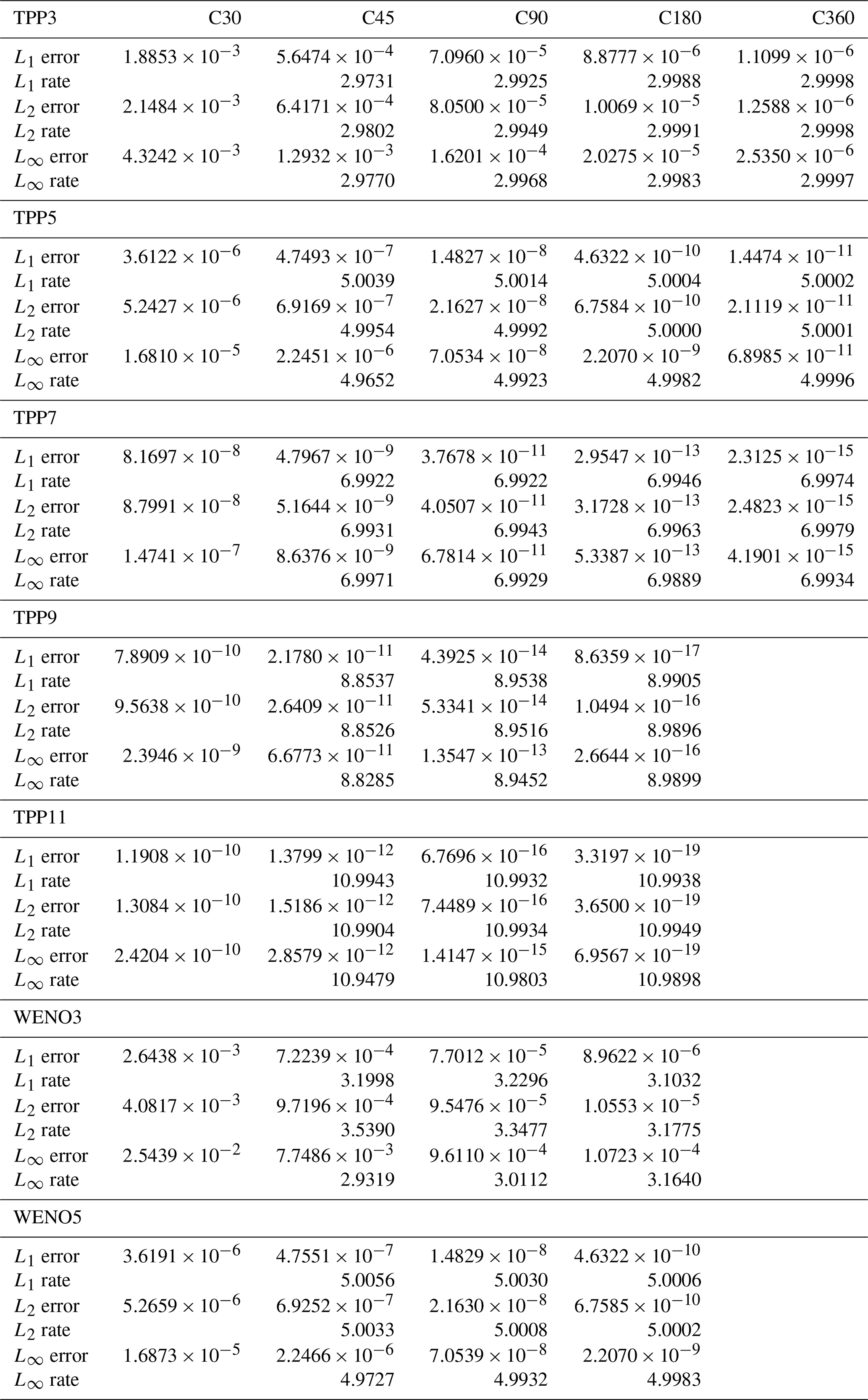
At lower resolutions, the simulation error of WENO3 is significantly higher than that of TPP3. However, as the resolution increases, the error of WENO3 progressively approaches that of TPP3. Comparing WENO5 and TPP5 results reveals a marginal increase in norm errors for WENO5, while maintaining 5th-order convergence rates. This confirms WENO5's capability to preserve high accuracy when simulating smooth flows.

It should be noted that HOPE achieves extremely small errors in simulating smooth flow fields even on very coarse resolutions. These errors can be so minute that they fall below the 16 significant digits representable in double precision. Under these conditions, conducting precision tests using double precision alone fails to accurately capture the true convergence rate. To obtain correct error measurements and convergence rate, we must employ FP128 (real (16) in Fortran). However, PyTorch's underlying architecture is built on NVIDIA CUDA, which currently supports only up to FP64 (double precision). Consequently, the PyTorch implementation cannot provide correct simulation errors when utilizing ultra-high-order schemes.

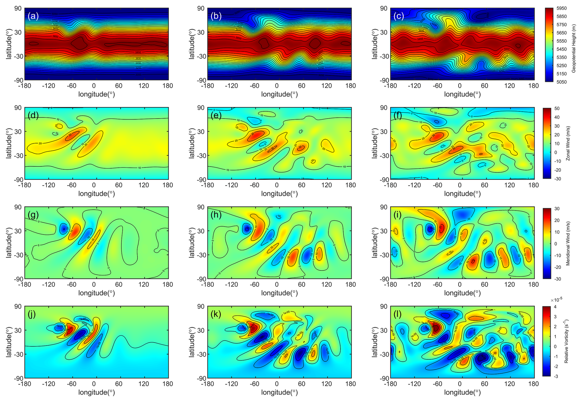
Figure 11 TPP5 (with LMARS) simulation result of the isolated mountain wave on C90 grid. The rows stand for variables: geopotential, zonal wind, meridional wind and relative vorticity, respectively. The columns represent simulation day 5, 10, 15. Geopotential contour from 5050 to 5950 m with interval 50 m. Zonal wind contour from −30 to 50 m s⁻¹ with interval 10 m s−1. Meridional wind contour from −30 to 30 m s⁻¹ with interval 10 m s⁻¹. Relative vorticity contour from $-\mathrm{3}\times {\mathrm{10}}^{-\mathrm{5}}$ to $\mathrm{4}\times {\mathrm{10}}^{-\mathrm{5}}$ s⁻¹ with interval $\mathrm{1}\times {\mathrm{10}}^{-\mathrm{5}}$ s⁻¹.

5.3 Zonal flow over an isolated mountain

Zonal flow over an isolated mountain is the 5th case mentioned in Williamson et al. (1992), this case was usually be implemented to test the topography influence in shallow water models. The initial condition is defined by Eqs. (79)–(81), but h₀=5960 m, ϕ₀=h₀g, u₀=20 m s⁻¹. The mountain height is expressed as

$$\begin{array}{}\text{(82)}& h_{\mathrm{s}}=h_{{\mathrm{s}}_{\mathrm{0}}}\left(\mathrm{1}-{\displaystyle \frac{d_{\mathrm{s}}}{R}}\right)\end{array}$$

where $h_{{\mathrm{s}}_{\mathrm{0}}}=\mathrm{2000}$ m; $R=\frac{\mathit{\pi }}{\mathrm{9}}$; $d_{\mathrm{s}}=\sqrt{\min [R^{\mathrm{2}},(\mathit{\lambda }-{\mathit{\lambda }}_{\mathrm{c}}{)}^{\mathrm{2}}+(\mathit{\theta }-{\mathit{\theta }}_{\mathrm{c}}{)}^{\mathrm{2}}]}$. ${\mathit{\lambda }}_{\mathrm{c}}=\frac{\mathrm{3}\mathit{\pi }}{\mathrm{2}}{\mathit{\theta }}_{\mathrm{c}}=\frac{\mathit{\pi }}{\mathrm{6}}$ are the center longitude and latitude of the mountain, respectively.

HOPE is able to deal with the bottom topography correctly, as shown in Fig. 11, all of the simulation result is consistent with prior researches such as (Nair et al., 2005a; Ullrich et al., 2010; Chen and Xiao, 2008) and so on. Furthermore, as discussed in Bao et al. (2014), some high order Discontinuous Galerkin (DG) method exhibit non-physical oscillation during simulating the over mountain flow, the additional viscosity operators are necessary to alleviate this issue. However, HOPE does not require any explicit viscosity operator to suppress vorticity oscillations, the vorticity fields are smooth all the time as illustrated in Fig. 11j–l. We have tested other schemes as well, including TPP3, TPP7, WENO3, and WENO5, all of the schemes are able to achieve similar simulation results.

In the 15 d simulation of zonal flow over an isolated mountain the total energy exhibited a gradual increase over the integration time, while the total potential enstrophy showed gradual dissipation as the simulation progressed. The AUSM⁺-up scheme demonstrated stronger energy dissipation compared to the LMARS scheme, as illustrated in Fig. 12.

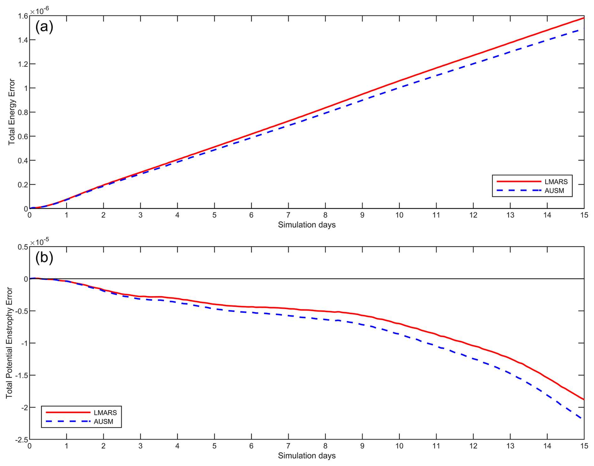
Figure 12 Time series of normalized conservation errors for the zonal flow over isolated mountain simulation on the C90 grid over days 0 to 15. (a) Normalized total energy error. (b) Normalized total potential enstrophy error. (c) Normalized total zonal angular momentum error.

5.4 Rossby–Haurwitz wave with 4 waves

Rossby–Haurwitz (RH) wave is the 6th test case introduced by Williamson et al. (1992), the RH waves are analytic solution of the spherical nonlinear barotropic vorticity equation, the reference solution is the zonal advection of RH wave without pattern changing, the angular phase speed is given by

$$\begin{array}{}\text{(83)}& c={\displaystyle \frac{R(R+\mathrm{3})\mathit{\omega }-\mathrm{2}\mathrm{\Omega }}{(R+\mathrm{1})(R+\mathrm{2})}}\end{array}$$

where R=4 is the zonal wavenumber, $\mathit{\omega }=\mathrm{7.848}\times {\mathrm{10}}^{-\mathrm{6}}$ s⁻¹; the earth rotation angular speed $\mathrm{\Omega }=\mathrm{7.292}\times {\mathrm{10}}^{-\mathrm{5}}$ s⁻¹. Therefore, we have the period T≈29.52 d. The initial condition expressed as

$$\begin{array}{}\text{(84)}& {\displaystyle }\mathit{\varphi }={\mathit{\varphi }}_{\mathrm{0}}+a^{\mathrm{2}}\left[A\left(\mathit{\theta }\right)+B\left(\mathit{\theta }\right)\cos R\mathit{\lambda }+C\left(\mathit{\theta }\right)\cos \mathrm{2}R\mathit{\lambda }\right]\text{(85)}& {\displaystyle }u=a\mathit{\omega }\cos \mathit{\theta }+aK{\cos }^{R-\mathrm{1}}\mathit{\theta }\left(R{\sin }^{\mathrm{2}}\mathit{\theta }-{\cos }^{\mathrm{2}}\mathit{\theta }\right)\cos R\mathit{\lambda }\text{(86)}& {\displaystyle }v=-aKR{\cos }^{R-\mathrm{1}}\mathit{\theta }\sin \mathit{\theta }\sin R\mathit{\lambda }\text{(87)}& {\displaystyle }\begin{array}{rl}A\left(\mathit{\theta }\right)=& {\displaystyle \frac{\mathit{\omega }}{\mathrm{2}}}(\mathrm{2}\mathrm{\Omega }+\mathit{\omega }){\cos }^{\mathrm{2}}\mathit{\theta }+{\displaystyle \frac{\mathrm{1}}{\mathrm{4}}}{K}^{\mathrm{2}}{\cos }^{\mathrm{2}R}\mathit{\theta }\\ & \left[(R+\mathrm{1}){\cos }^{\mathrm{2}}\mathit{\theta }+\mathrm{2}{R}^{\mathrm{2}}-R-\mathrm{2}-\mathrm{2}{R}^{\mathrm{2}}{\cos }^{-\mathrm{2}}\mathit{\theta }\right]\end{array}\text{(88)}& {\displaystyle }\begin{array}{rl}B\left(\mathit{\theta }\right)& ={\displaystyle \frac{\mathrm{2}(\mathrm{\Omega }+\mathit{\omega })K}{(R+\mathrm{1})(R+\mathrm{2})}}{\cos }^R\mathit{\theta }[R^{\mathrm{2}}+\mathrm{2}R+\mathrm{2}\\ & -(R+\mathrm{1}{)}^{\mathrm{2}}{\cos }^{\mathrm{2}}\mathit{\theta }]\end{array}\text{(89)}& {\displaystyle }C\left(\mathit{\theta }\right)={\displaystyle \frac{\mathrm{1}}{\mathrm{4}}}{K}^{\mathrm{2}}{\cos }^{\mathrm{2}R}\mathit{\theta }\left[(R+\mathrm{1}){\cos }^{\mathrm{2}}\mathit{\theta }-R-\mathrm{2}\right]\end{array}$$

where λ, θ are longitude and latitude, K=ω, ϕ₀=gh₀, h₀=8000 m, and a=6 371 220 m is the earth radius.

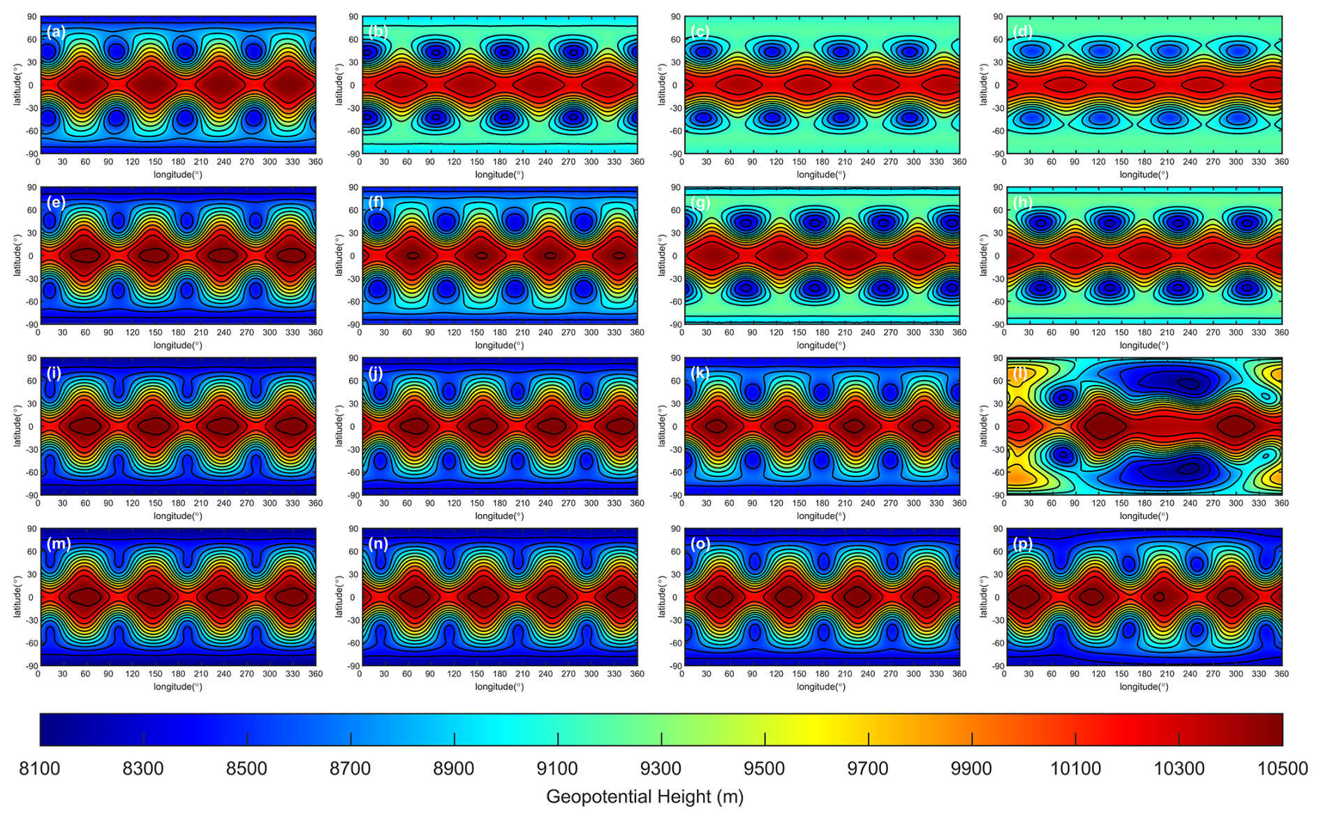
Figure 13 Geopotential of Rossby–Haurwitz wave simulated by TPP3 scheme. The rows represent grid C45, C90, C180 and C360, the columns stand for simulation day 14, 30, 60, 90. Contours from 8100 to 10 500 m with interval 200 m.

According to the study by Thuburn and Li (2000), the Rossby–Haurwitz (RH) wave with wavenumber 4 is inherently dynamically unstable and prone to collapse. This instability can be triggered by minute perturbations, such as those arising from grid structure (breaking initial symmetry), initial condition imperfections, or numerical errors (e.g., truncation or roundoff). Similar conclusions have been verified in subsequent research. In tests conducted by Zhou et al. (2020), the TRiSK framework based on the SCVT grid could only sustain the RH wave pattern for 25 d without collapse. In contrast, Li et al. (2020) successfully maintained the RH wave pattern for 89 d using a similar algorithm on a latitude-longitude grid. Ullrich et al. (2010) developed the high-order accuracy finite volume model based on a cubed-sphere grid, which was able to sustain the RH wave for up to 90 d. In the most of our experiments, the ability of HOPE to maintain the Rossby–Haurwitz (RH) wave significantly improved with increased order of accuracy and grid resolution. All of the simulation results are based on LMARS in this section.

In the TPP3 simulation, we found that the duration for which the RH wave is maintained increases with higher grid resolution, as exhibit in Fig. 13. When the grid resolution is low (C45, C90), an obvious dissipation phenomenon can be observed. When the resolution reaches C180, the dissipation is significantly reduced, but the waveform has completely collapsed by day 90. When the resolution reaches C360, the simulation results are further improved, with dissipation further reduced, and the RH wave waveform can still barely be maintained on day 90.

A 100 d simulation of the Rossby–Haurwitz wave was conducted using a C90 grid (1° resolution). The total energy simulated with the TPP3, TPP5, TPP7, and TPP9 schemes underwent dissipation to varying degrees. By day 100, the normalized total energy errors reached $-\mathrm{1.49}\times {\mathrm{10}}^{-\mathrm{3}}$, $-\mathrm{1.33}\times {\mathrm{10}}^{-\mathrm{5}}$, $-\mathrm{1.71}\times {\mathrm{10}}^{-\mathrm{6}}$, $-\mathrm{4.20}\times {\mathrm{10}}^{-\mathrm{7}}$, respectively, indicating significantly stronger dissipation for the TPP3 scheme compared to the other higher-order schemes (Fig. 14a). Figure 14b presents a scaled view of the energy evolution for TPP5, TPP7, and TPP9, clearly demonstrating that increasing the reconstruction order progressively reduces energy dissipation. Furthermore, following the RH wave collapse, a significant drop in total energy was observed for the TPP5 scheme (after approximately 90 d) and the TPP7 scheme (after approximately 95 d).

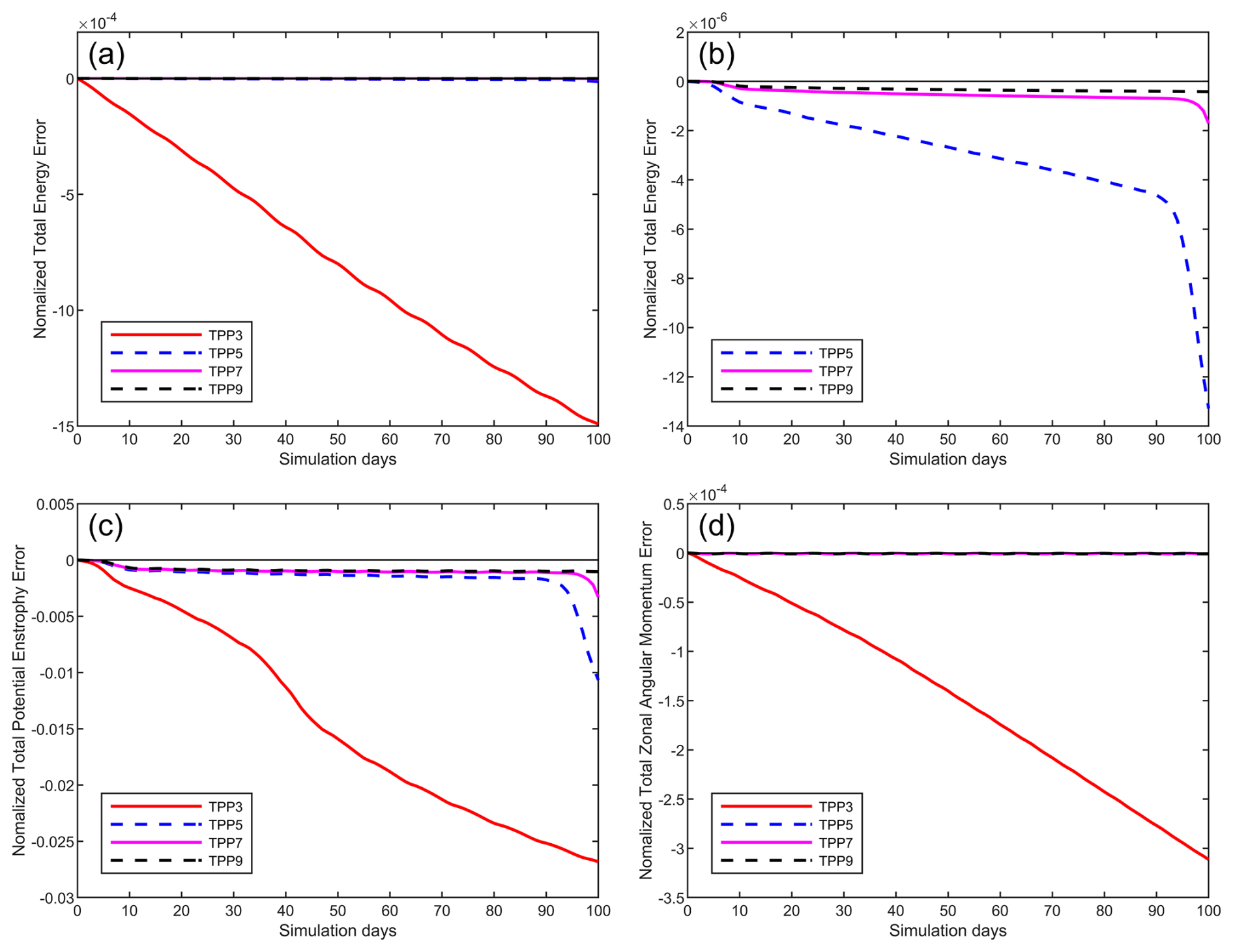
Figure 14 Time series of normalized conservation errors for the Rossby–Haurwitz wave simulation on the C90 grid over days 0 to 100, with LMARS scheme as Riemann solver. (a) Normalized total energy error for TPP3, TPP5, TPP7 and TPP9. (b) The total energy normalized error for TPP5, TPP7 and TPP9. (c) Normalized potential enstrophy error for TPP3, TPP5, TPP7 and TPP9. (d) Normalized total zonal angular momentum error for TPP3, TPP5, TPP7 and TPP9.

Analysis of the normalized total potential enstrophy error (Fig. 14c) and the normalized zonal angular momentum error (Fig. 14d) over time yields conclusions consistent with those for total energy. Specifically, the TPP3 scheme exhibited substantially higher dissipation than the higher-order schemes, confirming that employing higher-order reconstruction schemes effectively minimizes dissipation. Notably, significant dissipation surges occurred in these quantities following the RH wave collapse.

In Fig. 15, we compare the impact of order-of-accuracy on the simulation capability of RH waves by fixing the resolution. By comparing row by row, it can be observed that when the accuracy reaches 5th order or higher, the dissipation is significantly reduced. Both the TPP5 and TPP7 simulations show signs of waveform distortion on day 90, and the waveform completely collapses by day 100. However, when using TPP9 for the simulation, the waveform is well maintained even until day 100.

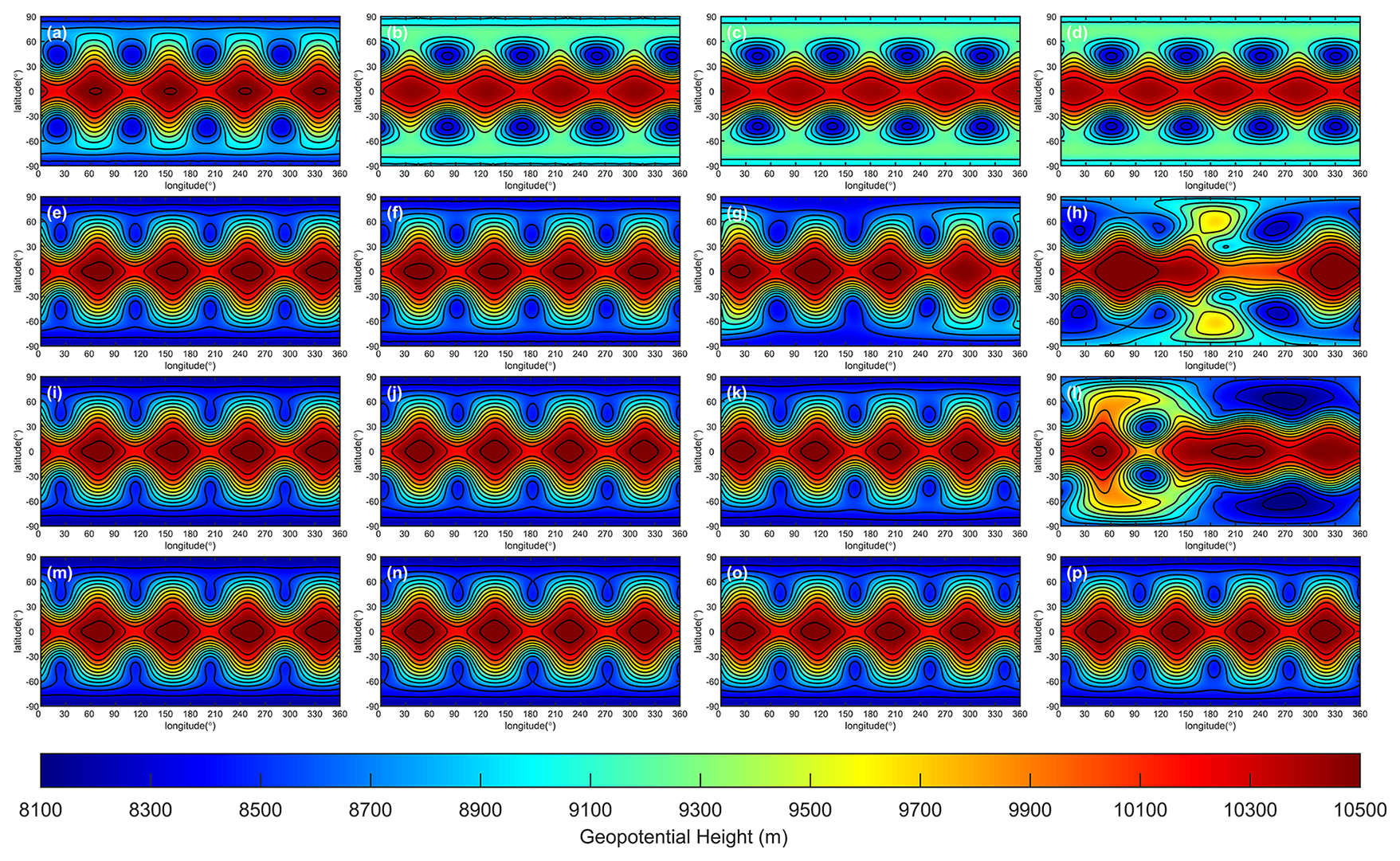
Figure 15 Geopotential of Rossby–Haurwitz wave on C90 grid, the rows represent the spatial reconstruction scheme with TPP3, TPP5, TPP7 and TPP9 the columns stand for simulation day 30, 60, 90 and 100. Contours from 8100 to 10 500 m with interval 200 m.

Figure 16 presents the simulation results on the 80th day for different resolutions and reconstruction schemes. The dissipation decreases as the resolution and reconstruction order improve. At the C45 resolution, both the TPP3 and TPP5 simulations exhibit significant dissipation. Although the TPP7 simulation shows a notable improvement in dissipation, the waveform is severely distorted. The TPP9 scheme produces the best simulation results. As the resolution increases, the simulation performance also improves significantly. When using the C360 resolution, all TPP schemes yield good simulation results.

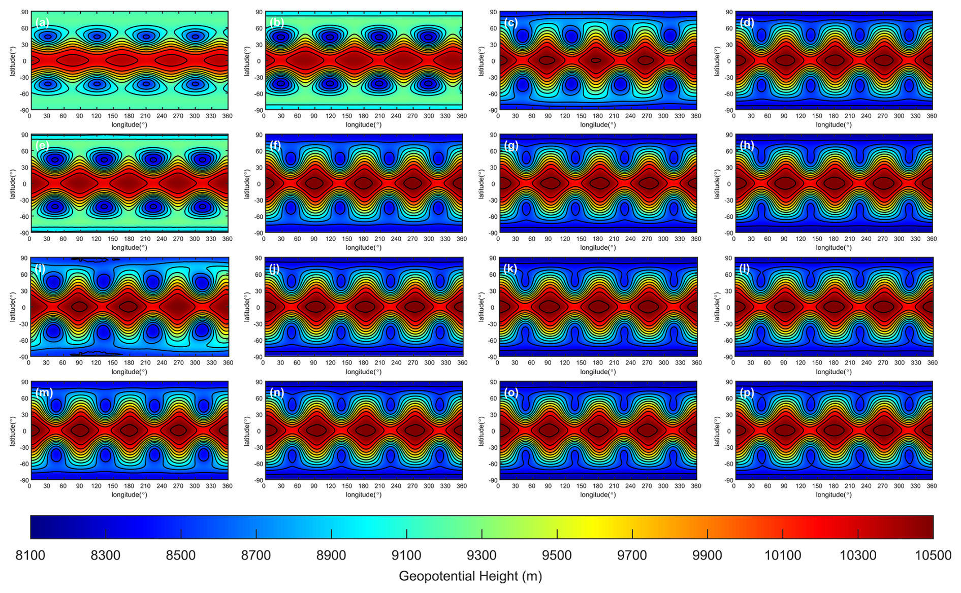
Figure 16 Geopotential of Rossby–Haurwitz wave at simulation day 80. The rows represent spatial reconstruction with TPP3, TPP5, TPP7 and TPP9. The columns stand for grid C45, C90, C180 and C360. Contours from 8100 to 10 500 m with interval 200 m.

Significant differences were observed between the 2D WENO scheme and the TPP schemes in this test. Regardless of the specific WENO order employed (3, 5, 7, or 9), all WENO variants maintained the Rossby–Haurwitz (RH) wave pattern for a shorter duration compared to their TPP counterparts of equivalent order. We infer that the nonlinear processes inherent within the WENO scheme introduce asymmetries that disrupt the computational stencil symmetry, leading to a premature collapse of the RH wave.

5.5 Perturbed jet flow

The perturbed jet flow was introduced by Galewsky et al. (2004), this experiment was desired to test the model ability of simulating the fast and slow motion. the initial field is defined as

$$\begin{array}{}\text{(90)}& {\displaystyle }& {\displaystyle }u\left(\mathit{\theta }\right)=\left\{\begin{array}{ll}\frac{u_{\max }}{e_{\mathrm{n}}}{e}^{\frac{\mathrm{1}}{\left(\mathit{\theta }-{\mathit{\theta }}_{\mathrm{0}}\right)\left(\mathit{\theta }-{\mathit{\theta }}_{\mathrm{1}}\right)}},& \mathit{\theta }\in \left({\mathit{\theta }}_{\mathrm{0}},{\mathit{\theta }}_{\mathrm{1}}\right)\\ \mathrm{0},& \mathrm{otherwise}\end{array}\right.\text{(91)}& {\displaystyle }& {\displaystyle }\mathit{\varphi }(\mathit{\lambda },\mathit{\theta })={\mathit{\varphi }}_{\mathrm{0}}+{\mathit{\varphi }}^{\prime }(\mathit{\lambda },\mathit{\theta })-\underset{-\frac{\mathit{\pi }}{\mathrm{2}}}{\overset{\mathit{\theta }}{\int }}au\left({\mathit{\theta }}^{\prime }\right)\left[f+{\displaystyle \frac{\tan {\mathit{\theta }}^{\prime }}{a}}u\left({\mathit{\theta }}^{\prime }\right)\right]\mathrm{d}{\mathit{\theta }}^{\prime }\text{(92)}& {\displaystyle }& {\displaystyle }{\mathit{\varphi }}^{\prime }(\mathit{\lambda },\mathit{\theta })=g\widehat{h}\cos \mathit{\theta }{e}^{-{\left(\frac{\mathit{\lambda }}{\mathit{\alpha }}\right)}^{\mathrm{2}}-{\left(\frac{{\mathit{\theta }}_{\mathrm{2}}-\mathit{\theta }}{\mathit{\beta }}\right)}^{\mathrm{2}}},\mathit{\lambda }\in (-\mathit{\pi },\mathit{\pi })\end{array}$$

where λ, θ represents longitude and latitude, a=6 371 220 m is radius of earth, u_max=80 m s⁻¹, ${\mathit{\theta }}_{\mathrm{0}}=\frac{\mathit{\pi }}{\mathrm{7}}$, ${\mathit{\theta }}_{\mathrm{1}}=\frac{\mathrm{5}\mathit{\pi }}{\mathrm{14}}$, ${\mathit{\theta }}_{\mathrm{2}}=\frac{\mathit{\pi }}{\mathrm{4}}$, $e_{\mathrm{n}}=e^{\frac{-\mathrm{4}}{({\mathit{\theta }}_{\mathrm{1}}-{\mathit{\theta }}_{\mathrm{0}}{)}^{\mathrm{2}}}}$, $\mathit{\alpha }=\frac{\mathrm{1}}{\mathrm{3}}$, $\mathit{\beta }=\frac{\mathrm{1}}{\mathrm{15}}$, and $\widehat{h}=\mathrm{120}$ m. We adopt LMARS as Riemann solver in all of the simulation in this section.

As mentioned in Chen and Xiao (2008), the perturbed jet flow experiment poses a particular challenge for the cubed-sphere grid model. Firstly, the jet stream is located at 45° N, which is very close to the boundaries of panel 5 of the cubed-sphere grid, resulting in a large geopotential gradient in the ghost interpolation region, which leads to larger interpolation error. Furthermore, the location of the geopotential perturbation ϕ^′ coincides with the boundary between panel 1 and panel 5, which also leads to greater numerical computation errors.

Figure 17 displays the HOPE simulation outcomes at day 6 for varying levels of reconstruction order and resolutions. The four rows correspond to the TPP5, TPP7, TPP9 and TPP11 schemes in terms of reconstruction order. The three columns, meanwhile, represent the resolutions of C45, C90, and C180, respectively. Upon comparing the different columns, it is evident that the perturbed jet flow test case converges as the resolution increases. Figure 17a, d, g, and j illustrate that, with an increase in reconstruction order, the vorticity field patterns become increasingly similar to the high-resolution results shown in the second and third columns of Fig. 17. Notably, HOPE enhances the simulation results by utilizing both higher reconstruction order and higher resolution.

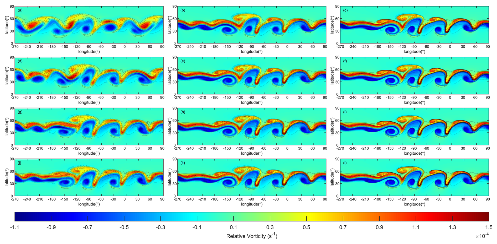
Figure 17 Relative vorticity of perturbed jet flow. (a)–(c) represent the results of TPP5 scheme with resolutions C45, C90, C180. (d)–(f) represent the results of TPP7 scheme with resolutions C45, C90, C180. (g)–(i) represent the results of TPP9 scheme with resolutions C45, C90, C180. (j)–(l) represent the results of TPP11 scheme with resolutions C45, C90, C180.

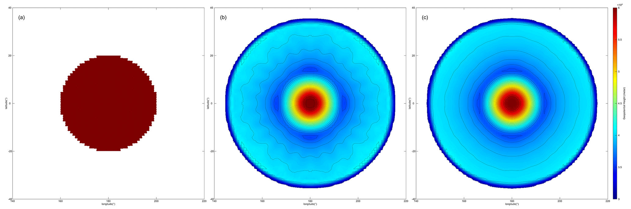
Figure 18 Geopotential of dam-break test case on C90 grid at 2nd hour. (a) Initial condition, (b) WENO 1D, (c) WENO 2D. The horizontal resolution for both schemes is C90. Shaded and contour from 3.2×10⁴ to 6×10⁴ m, with contour interval 10³ m.

5.6 Dam-break shock wave

In this section we introduce a dam-break case for testing the capability of HOPE to capture the shock wave and comparing the difference between 1D and 2D WENO schemes. The initial condition is configured as a cylinder with a geopotential of 30 000 m² s⁻², as shown in Fig. 18a. The geopotential is given by

$$\begin{array}{}\text{(93)}& \mathit{\varphi }\left(d_{\mathrm{s}}(\mathit{\lambda },\mathit{\theta })\right)=\left\{\begin{array}{ll}\mathrm{2}{\mathit{\varphi }}_{\mathrm{0}},& r<r_{\mathrm{c}}\\ {\mathit{\varphi }}_{\mathrm{0}},& \mathrm{otherwise}\end{array}\right.\end{array}$$

where $d_{\mathrm{s}}=\sqrt{(\mathit{\lambda }-{\mathit{\lambda }}_{\mathrm{c}}{)}^{\mathrm{2}}+(\mathit{\theta }-{\mathit{\theta }}_{\mathrm{c}}{)}^{\mathrm{2}}}{\mathit{\lambda }}_{\mathrm{c}}=\mathit{\pi }$, θ_c=0, $r_{\mathrm{c}}=\frac{\mathit{\pi }}{\mathrm{9}}$, ϕ₀=30 000 m² s⁻², and the earth rotation angular speed Ω=0. We adopt LMARS as Riemann solver in all of the simulation in this section.

In this experiment, we compare WENO5 (WENO scheme with reconstruction width 5) on both 1D and 2D schemes, the WENO-Z (Borges et al., 2008) is adopted as WENO 1D scheme, and WENO 2D scheme is consist with Sect. 3.2. Due to the initial condition being a cylinder, the resulting shock wave should maintain a circular feature. In the simulation results of WENO 1D, numerous radial textures appear (Fig. 18b). The simulation results using the WENO 2D scheme exhibit a smoother circular shape, Fig. 18c. This outcome arises because the 1D reconstruction scheme suffers from dimension split error, whereas the fitting function in the 2D reconstruction scheme incorporates cross terms. Therefore, when simulating fluid fields characterized by isotropic features, the 1D scheme lacks the capability to accurately represent diagonal directional features. Conversely, the 2D scheme correctly captures the inherent isotropic characteristics.

6 Conclusions

This paper presents HOPE, an innovative finite-volume model capable of achieving arbitrary odd-order convergence rate. Through comprehensive numerical experiments, we demonstrate that HOPE exhibits excellent convergence properties when applied to smooth flow fields, with simulation errors decreasing rapidly as the order of accuracy increases.

The model's performance has been rigorously evaluated across several benchmark cases:

1. In Rossby–Haurwitz wave simulations, HOPE demonstrates superior waveform preservation capabilities that scale with both spatial resolution and accuracy order.

2. For perturbed jet flow scenarios, the model successfully resolves both fast and slow dynamical features, with significant improvements in solution quality observed at higher orders and finer resolutions.

3. Mountain wave simulations confirm HOPE's ability to accurately represent orographically-forced gravity waves.

4. In the dam break test case featuring cylindrical shock fronts, the two-dimensional WENO reconstruction scheme proves more effective than dimension-split approaches in maintaining circular symmetry.

In the case of steady geostrophic flow, Both WENO3 and WENO5 achieve the expected 3rd-order and 5th-order convergence rates, respectively. However, the computed norm errors for WENO schemes are marginally larger than those obtained with the TPP3 and TPP5 schemes. This observation confirms that the 2D WENO scheme preserves the designed convergence rate in smooth flow regions. Concurrently, in the Dam-Break Shock Wave case, the 2D WENO scheme demonstrates its robust capability for handling discontinuous flow fields. These combined results align perfectly with the primary motivation for introducing the WENO scheme: its adaptive oscillation suppression capability. Specifically, the scheme preserves the high convergence rate in sufficiently smooth regions while automatically reducing the reconstruction order near discontinuities to effectively suppress the development and propagation of non-physical oscillations.

A key innovation of HOPE lies in its computational architecture. The algorithm is specifically designed to harness GPU acceleration through (1) implementation of spatial reconstructions as convolutional operations, and (2) formulation of integration steps as matrix-vector products. These design choices leverage computational patterns widely adopted in machine learning frameworks. By developing HOPE within PyTorch, we inherit automatic differentiation capabilities, enabling straightforward coupling with neural network systems.

This integration facilitates the development of hybrid prediction models that combine a high-order, high-performance dynamical core, and Neural network-based physical parameterizations. Current research efforts have successfully extended this algorithmic framework to a two-dimensional baroclinic model (X–Z dimensions).

Future work will focus on developing a global, fully compressible baroclinic model using the HOPE algorithm, further demonstrating its versatility and advantages for modeling complex atmospheric dynamics. The model's unique combination of physical conservation, computational efficiency, and machine learning compatibility positions it as a powerful tool for next-generation atmospheric modeling.

Appendix A

In this appendix, we introduce a novel boundary ghost cell interpolation scheme for cubed sphere, which is able to support HOPE to reach the accuracy over 11th order or even higher.

There are two types of cells, in-domain and out-domain (also named ghost cell, as show in Fig. 7b), we define the set of in-domain cell values ${\mathit{q}}_{d\times \mathrm{1}}=(q_{\mathrm{1}},q_{\mathrm{2}},\mathrm{\dots },q_d{)}^T$, the set of out-domain cell values ${\mathit{g}}_{h\times \mathrm{1}}=(g_{\mathrm{1}},g_{\mathrm{2}},\mathrm{\dots },g_d{)}^T$, and the set of Gaussian quadrature point values (green points in Fig. 3) in out-domain cells is define as ${\mathit{v}}_{p\times \mathrm{1}}=(v_{\mathrm{1}},v_{\mathrm{2}},\mathrm{\dots },v_p)$. To identify the shape of the arrays, we denote the array shape using subscripts (this convention will be followed throughout the subsequent text). The purpose of ghost cell interpolation is using the known cell value q to interpolate the unknown g.

Define a new set includes the values of domain cell values and ghost cell values

$$\begin{array}{}\text{(A1)}& {\stackrel{\mathrm{̃}}{\mathit{q}}}_{(d+h)\times \mathrm{1}}=\mathit{q}\bigcup \mathit{g}={\left(q_{\mathrm{1}},q_{\mathrm{2}},\mathrm{\dots },q_d,g_{\mathrm{1}},g_{\mathrm{2}},\mathrm{\dots },g_h\right)}^T\end{array}$$

Similar to the describe in section 0, we can use a TPP to reconstruct the ghost quadrature points

$$\begin{array}{}\text{(A2)}& {\mathit{v}}_{p\times \mathrm{1}}={\mathbf{A}}_{p\times (d+h)}{\stackrel{\mathrm{̃}}{\mathit{q}}}_{(d+h)\times \mathrm{1}}\end{array}$$

where ${\mathbf{A}}_{p\times (d+h)}$ is the interpolation matrix that can be obtain by the similar method to Eq. (29). The ghost cell values are calculated by Gaussian quadrature

$$\begin{array}{}\text{(A3)}& {\mathit{g}}_{h\times \mathrm{1}}={\mathbf{B}}_{h\times p}{\mathit{v}}_{p\times \mathrm{1}}\end{array}$$

where B_h×p is the Gaussian quadrature matrix.

${\stackrel{\mathrm{̃}}{\mathit{q}}}_{(d+h)\times \mathrm{1}}$ can be decomposed as the linear q_d×1 and v_p×1

$$\begin{array}{}\text{(A4)}& \begin{array}{rl}{\stackrel{\mathrm{̃}}{\mathit{q}}}_{(d+h)\times \mathrm{1}}& =\left(\begin{array}{ll}{\mathbf{I}}_{d\times d}& \mathrm{0}\\ \mathrm{0}& {\mathbf{B}}_{h\times p}\end{array}\right)\left(\begin{array}{c}{\mathit{q}}_{d\times \mathrm{1}}\\ {\mathit{v}}_{p\times \mathrm{1}}\end{array}\right)\\ & ={\stackrel{\mathrm{̃}}{\mathbf{B}}}_{(d+h)\times (d+p)}{\stackrel{\mathrm{‾}}{\mathit{q}}}_{(d+p)\times \mathrm{1}}\end{array}\end{array}$$

where I_d×d is an identity matrix, and

$$\begin{array}{}\text{(A5)}& {\displaystyle }& {\displaystyle }{\stackrel{\mathrm{̃}}{\mathbf{B}}}_{(d+h)\times (d+p)}=\left(\begin{array}{ll}{\mathbf{I}}_{d\times d}& \mathrm{0}\\ \mathrm{0}& {\mathbf{B}}_{h\times p}\end{array}\right)\text{(A6)}& {\displaystyle }& {\displaystyle }{\stackrel{\mathrm{‾}}{\mathit{q}}}_{(d+p)\times \mathrm{1}}=\left(\begin{array}{c}{\mathit{q}}_{d\times \mathrm{1}}\\ {\mathit{v}}_{p\times \mathrm{1}}\end{array}\right).\end{array}$$

Substitute Eq. (30) into Eq. (26), we have

$$\begin{array}{}\text{(A7)}& \begin{array}{rl}{\mathit{v}}_{p\times \mathrm{1}}& ={\mathbf{A}}_{p\times (d+h)}{\stackrel{\mathrm{̃}}{\mathbf{B}}}_{(d+h)\times (d+p)}{\stackrel{\mathrm{‾}}{\mathit{q}}}_{(d+p)\times \mathrm{1}}\\ & ={\stackrel{\mathrm{̃}}{\mathbf{A}}}_{p\times (d+p)}{\stackrel{\mathrm{‾}}{\mathit{q}}}_{(d+p)\times \mathrm{1}}={\stackrel{\mathrm{̃}}{\mathbf{A}}}_{p\times (d+p)}\left(\begin{array}{c}{\mathit{q}}_{d\times \mathrm{1}}\\ {\mathit{v}}_{p\times \mathrm{1}}\end{array}\right).\end{array}\end{array}$$

We found that matrix ${\stackrel{\mathrm{̃}}{\mathbf{A}}}_{p\times (d+p)}$ can be decomposed into two parts

$$\begin{array}{}\text{(A8)}& {\stackrel{\mathrm{̃}}{\mathbf{A}}}_{p\times (d+p)}=\left(\begin{array}{cc}{\stackrel{\mathrm{‾}}{\mathbf{A}}}_{p\times d}& {\mathbf{C}}_{p\times p}\end{array}\right).\end{array}$$

Such that

$$\begin{array}{}\text{(A9)}& {\mathit{v}}_{p\times \mathrm{1}}={\stackrel{\mathrm{‾}}{\mathbf{A}}}_{p\times d}{\mathit{q}}_{d\times \mathrm{1}}+{\mathbf{C}}_{p\times p}{\mathit{v}}_{p\times \mathrm{1}}.\end{array}$$

Therefore

$$\begin{array}{}\text{(A10)}& \left({\mathbf{I}}_{p\times p}-{\mathbf{C}}_{p\times p}\right){\mathit{v}}_{p\times \mathrm{1}}={\stackrel{\mathrm{‾}}{\mathbf{A}}}_{p\times d}{\mathit{q}}_{d\times \mathrm{1}}.\end{array}$$

We set ${\mathbf{D}}_{p\times p}={\mathbf{I}}_{p\times p}-{\mathbf{C}}_{p\times p}$, then v_p×1 can be determined by

$$\begin{array}{}\text{(A11)}& {\mathit{v}}_{p\times \mathrm{1}}={\mathbf{D}}_{p\times p}^{-\mathrm{1}}{\stackrel{\mathrm{‾}}{\mathbf{A}}}_{p\times d}{\mathit{q}}_{d\times \mathrm{1}}.\end{array}$$

Substitute Eq. (A11) into Eq. (A3), we establish the relationship between ghost cell values and in-domain cell values

$$\begin{array}{}\text{(A12)}& \begin{array}{rl}{\mathbf{g}}_{h\times \mathrm{1}}& ={\mathbf{B}}_{h\times p}{\mathit{v}}_{p\times \mathrm{1}}={\mathbf{B}}_{h\times p}{\mathbf{D}}_{p\times p}^{-\mathrm{1}}{\stackrel{\mathrm{‾}}{\mathbf{A}}}_{p\times d}{\mathit{q}}_{d\times \mathrm{1}}\\ & ={\mathcal{G}}_{h\times d}{\mathit{q}}_{d\times \mathrm{1}}\end{array}\end{array}$$

where ${\mathcal{G}}_{h\times d}={\mathbf{B}}_{h\times p}{\mathbf{D}}_{p\times p}^{-\mathrm{1}}{\stackrel{\mathrm{‾}}{\mathbf{A}}}_{p\times d}$. It is clear that Eq. (A.12) is linear, and only rely on the mesh and Gaussian quadrature scheme. Therefore, we need to compute the projection matrix 𝒢_h×d only once for a given mesh and accuracy, this matrix can be computed by a preprocessing system and save it to the hard disk.