A Python diagnostics package for evaluation of Madden–Julian Oscillation (MJO) teleconnections in subseasonal-to-seasonal (S2S) forecast systems

The Madden–Julian Oscillation (MJO) teleconnections diagnostics package is an open-source Python software package that provides process-level evaluation of MJO teleconnections predicted by subseasonal-to-seasonal (S2S) forecast systems. The package provides in-depth process-level evaluation of both tropospheric and stratospheric pathways defining the atmospheric teleconnections from the tropics to the extratropics on S2S time scales. The analyses include the comparison of a forecast model with a default verification dataset or user-provided verification data. The package consists of a user-friendly graphical user interface (GUI), which allows the package to be applied to both operational and research models. This approach allows for efficient data management and the reproducibility of the analysis.

1 Introduction

S2S forecasting is an activity that bridges the gap between medium-range weather forecasting (lead time 1–2 weeks) and seasonal forecasting (lead time 1–3 months). In this time range, the main sources of predictability transition from the memory of initial conditions to the boundary conditions forcing. As a result, other sources of predictability are tapped into for enhancing the forecast skill for weeks 3–4 lead time. One of the sources of predictability, especially for boreal winters, has been identified as the extratropical response to the Madden–Julian Oscillation (MJO; Madden and Julian, 1971, 1972) activity in the tropical atmosphere. The MJO signal reaches the Northern Hemisphere (NH) midlatitudes via barotropic Rossby waves (Jin and Hoskins, 1995; Wang and Xie, 1996), channeled through a waveguide in the upper troposphere and/or through stratosphere–troposphere coupling. Teleconnections following the “tropospheric pathway” have a global impact, with the strongest influence on the Pacific North American sector's surface weather (Higgins et al., 2000; Cassou, 2008; Lin et al., 2009; Zhou et al., 2012; Riddle et al., 2013; Johnson et al., 2014). Teleconnections following the “stratospheric pathway” influence the surface weather of the North Atlantic and Europe. They can constructively interact with the teleconnections through the upper troposphere, amplifying the response to MJO forcing. This results in a stronger and more long-lasting effect (Schwartz and Garfinkel, 2017; Green and Furtado, 2019).

The MJO is the dominant large-scale atmospheric circulation pattern of intraseasonal variability (30–90 d) in the tropics. A typical event manifests as a “pulse” of cloud and rainfall that moves eastward at about 4–8 m s⁻¹ and recurs every 40 to 60 d (Madden and Julian, 1971, 1972). The MJO has its primary peak season in boreal winter, when the strongest signals are located south of the Equator; the secondary peak season is in boreal summer, when the strongest signals are located north of the Equator (Zhang, 2005). The amplitude and phase of MJO events can be described using the Real-time Multivariate MJO (RMM) index (Wheeler and Hendon, 2004). The life cycle of an MJO event is divided into eight phases, described by the location of increased cloudiness and rainfall (active convection) as follows: in phase 1, it begins over the western Indian Ocean; in phase  2, it moves eastward to the central Indian Ocean; in phase 3, it reaches the eastern Indian Ocean and Maritime Continent; in phase 4, it spreads over the Maritime Continent; in phase 5, it moves over the far-western Pacific; in phase 6, it spreads over the western-central Pacific Ocean; in phase 7, it moves to the central Pacific Ocean; and in phase 8, it reaches the western hemisphere and Africa, thereby completing the cycle.

The Rossby waves form in response to perturbations induced by moist diabatic processes associated with tropical convection (Teng and Branstator, 2019), which often aggregates into the MJO. The waves are generated by the so-called Rossby wave sources (Sardeshmukh and Hoskins, 1988) or by basic state vorticity gradients. The MJO heating leads to horizontal divergence of the wind in the upper troposphere and changes in the rotational wind. The wave activity emanating from the source propagates eastward and poleward. While the waveguide is modulated by the position of jet streams (Enomoto et al., 2003), it can also be influenced by the anomalous cyclonic and anticyclonic upper-level circulations induced by the waves (Zheng et al., 2018).

The waves with zonal wavenumber 1 and wavenumber 2 play the most important role in the stratosphere–troposphere coupling as they transit the tropopause and reach the polar stratosphere (Charney and Drazin, 1961; Weinberger et al., 2022). The heat and momentum fluxes transported by these waves can be absorbed within the stratospheric polar vortex, modifying the strength of the vortex (Chen and Robinson, 1992; Limpasuvan et al., 2004; Polvani and Waugh, 2004; White et al., 2019; Weinberger et al., 2022). Perturbations in the vortex are often associated with changes in the large-scale circulation patterns at the surface in the following weeks (Baldwin and Dunkerton, 1999; Polvani and Kushner, 2002; Polvani and Waugh, 2004; White et al., 2019; Baldwin et al., 2021).

The impact of the MJO on the extratropics is stronger during boreal winter and manifests as regional modulations of circulation, temperature, and precipitation (Stan et al., 2017) across the entire NH (Yoneyama and Zhang, 2020). The response of the extratropics to MJO forcing is established on a two-week time scale (Jin and Hoskins, 1995) and depends on the MJO phases described by the location of active and suppressed convection. Stan et al. (2017) provide a review of mechanisms underpinning the tropical-extratropical teleconnections.

Given the broad impact of the MJO on global weather/climate systems, acting as a major source of global S2S predictability, this paper introduces a new Python package that consists of metrics and diagnostics for the evaluation of the MJO and processes driving the MJO teleconnections in forecast data. The scientific basis of the diagnostics included in the package has been documented in the literature. The diagnostics have been applied to forecast systems in the S2S database (Stan et al., 2022) and the prototypes of the NOAA UFS global coupled model (Zheng et al., 2024; Garfinkel et al., 2024; Wang et al., 2025).

The objective of the paper is to guide users on how to apply the package to their forecast data, to understand the strengths and weaknesses of a forecast system in predicting the mechanisms driving the MJO teleconnections compared to their observed characteristics, and to provide a limited deterministic evaluation of the forecast skill. Additionally, the package provides a tool for the evaluation of the MJO forecast skill. Due to the delayed response of the extratropics to MJO forcing, evaluation of MJO teleconnections by forecast systems is conducted with respect to the presence of MJO events in initial conditions, which allows the use of reanalysis/observation-based products for event description.

The package consists of a graphical user interface (GUI) and a collection of modular evaluation tools, all written in Python v3.9.16 and its associated scientific libraries. The package can be applied to any forecast dataset prepared in the specified format. The basic concept of the diagnostics package is similar to other community-contributed metrics packages, such as the PCMDI Metric Package (PMP; Glecker et al., 2008, 2016; Lee et al., 2024), the Toolkit for Extreme Climate Analysis (TECA), the international Land Model Benchmarking Tool (ILAMB; Collier et al., 2018), the International Ocean Model Benchmarking (IOMB) package operating under the umbrella of the Coordinated Model Evaluation Capabilities (CMEC), the Process-oriented diagnostics (PODs) coordinated by the Model Diagnostics Task Force (MDTF; Neelin et al., 2023), the Climate Variability and Diagnostics Package (CDVP; Phillips et al., 2014; Maher et al., 2025), the Atmosphere Model Working Group (AMWG) Diagnostics Framework (ADF), and others. The major difference between these diagnostics packages and the MJO teleconnections diagnostics package is that the latter is tailored for S2S forecast data, which typically extend to no more than 46 d (Vitart et al., 2017). The other packages apply to multi-century climate simulations.

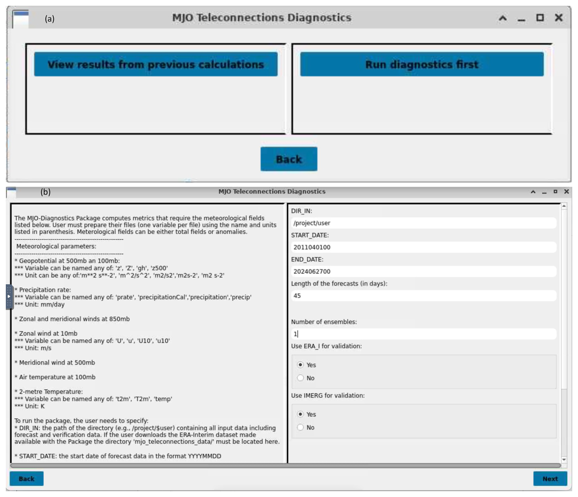
Figure 1 Window-based structure of GUI. (a) Selection of function mode. (b) Window collecting user input for running diagnostics.

2 Components of the diagnostics package

2.1 The graphical user interface

The user interface provides two primary functions: (i) selecting and running diagnostics and (ii) displaying existing results (Fig. 1a). The interface is built using PyQt5, a popular Python framework for creating GUIs. The GUI features a window-based design organized into a sequence of menus with two sections. The static section provides help text, while the dynamic section contains input containers and buttons for user interaction (Fig. 1b).

By providing quick information, the help text reduces the need to consult external documentation. Users can navigate back and forth between windows, allowing for a flexible workflow.

The diagnostics can be applied to a single forecast dataset, which can be compared against a default dataset or user-provided verification data. The default datasets are the ECMWF Reanalysis (ERA) Interim (Dee et al., 2011) for wind, geopotential, and 2 m temperature and the Integrated Multi-satellitE Retrievals for GPM (IMERG; Huffman et al., 2014) for precipitation.

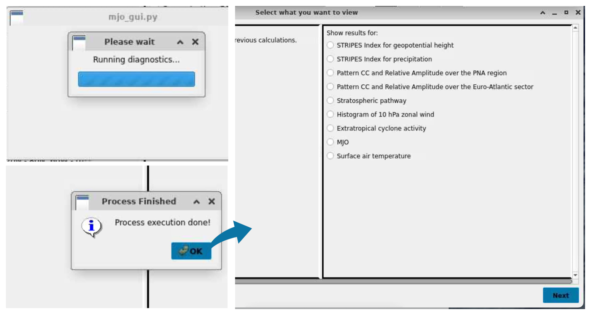
The user inputs collected through the GUI are saved as dictionaries in a YAML configuration file. Then, each diagnostic reads relevant entries from this configuration. This approach gives the package flexibility and extensibility. The design allows for the easy addition of new diagnostics. Users can choose from various diagnostic options, and the interface allows running a single diagnostic, a subset, or all available diagnostics. After the computation of the diagnostics has been completed, the interface opens a new window for displaying the results of all computed diagnostics (Fig. 2). Figures and, in some cases, data files can then be saved locally.

Figure 2 GUI windows illustrating the computational stage of the diagnostics.

The GUI offers additional options, such as computing or using pre-computed model anomalies, using the default RMM index or a user-provided index, and specifying forecast details, such as the time period, length, and number of ensembles. Help text is provided to guide users on file formats, names, and variable names and units (Table A1 provides a list of accepted variable names and units).

Windows displaying results contain comprehensive explanations of the main features emphasized by the diagnostic. This format allows users with different abilities to use the diagnostics, reducing the need to consult external documentation. Having the result of each diagnostic available in a stand-alone window allows users to compare diagnostic results simultaneously.

The GUI has built-in features that prevent users from entering invalid data. For example, no field can have a null value, and users are prompted with additional information about the missing input.

It is also possible to select and run diagnostics without the GUI. In non-GUI mode, users can directly specify diagnostic settings in a YAML configuration file, which the package reads to run the desired diagnostics. The same capabilities are available in non-GUI mode as in the GUI version, ensuring consistency across different usage modes and allowing for automation, batch processing, and integration into larger workflows without the need for manual interaction with the graphical interface.

2.2 Diagnostics

The MJO teleconnections codebase is designed to be modular, and each diagnostic set is self-contained. They share common tools such as horizontal interpolation, the computation of climatology, and anomalies. Each diagnostic tool has its own main Python script that is invoked by the GUI and reads the user input from the configuration YAML file. The output from each diagnostic, including figures and tables, is organized in a user-defined directory and can be displayed in the GUI.

All diagnostics require data in the network Common Data Form (netCDF) format using CF Metadata conventions (Eaton et al., 2024). Forecast data must be organized as one experiment per file and per ensemble member for diagnostics requiring calculations for individual ensemble members. If the forecast is compared with ERA Interim (ERAI) and IMERG and the horizontal resolution of the forecast data is higher than the verification data, each diagnostic interpolates the forecast data to the ERAI grid (512 longitude grid points ordered from 0 to 360°, 256 latitude grid points ordered from 90° N to 90° S) and the IMERG grid (480 longitude grid points ordered from 0 to 360°, 241 latitude grid points ordered from 90° S to 90° N), respectively. The stored direction of the latitude in the forecast data can be either decreasing or increasing. If the horizontal resolution of the forecast data is coarser than that of verification data, the interpolation is to the grid of forecast data. The code ensures that regridding is always from the high- to low-resolution grid. The regridding algorithm is Python Spherical Harmonic Transform Module, pysharm 1.0.9 (Whitaker, 2020), which is built on the collection of FORTRAN programs SPHEREPACK (Adams and Swartztrauber, 1999). Verification data can also be user specified and in that case, the grid must match the grid of the forecast data. The package does not have the capability to directly compare two sets of forecast data. In all diagnostics, the MJO phases are defined based on the MJO phase characterizing the initial date of the forecast. Users have the option to use the RMM index based on ERAI or provide new index data.

The meteorological parameters used by the package include geopotential or geopotential height at 500 and 100 hPa, (Z₅₀₀ and Z₁₀₀), temperature at 500 and 100 hPa (T₅₀₀ and T₁₀₀), the zonal and meridional components of the wind at 850 hPa (U₈₅₀ and V₈₅₀), zonal wind at 10 hPa (U₁₀), meridional component of the wind at 500 hPa (V₅₀₀), zonal component of the wind at 200 hPa (U₂₀₀), 2 m temperature (T2m), surface precipitation rate (PREC), and outgoing longwave radiation (OLR) at the top of the atmosphere. Table A1 provides accepted names of variables and their units. All diagnostics with the exception of one require data at a daily frequency. The forecast data must consist of a minimum of 35 d.

In all diagnostics, the MJO teleconnections are evaluated during boreal winter (November through March). For diagnostics that include statistical significance, a bootstrap method using 1000 samples is employed for its computation.

2.2.1 STRIPES index

The Remote Influence of Periodic EventS (STRIPES) index was introduced by Jenney et al. (2019) to characterize the regional impact of aggregated MJO phases, each assumed to last approximately 5 to 7 d. The STRIPES index measures the MJO teleconnections as the covariability between the MJO activity and regional fluctuations of meteorological parameters. It takes into account both the magnitude and consistency of the MJO's influence across multiple events. The STRIPES index takes values between 1 and +∞. It reaches high values when two conditions are met: first, the meteorological parameter shows a strong correlation with the MJO activity, and second, this relationship remains consistent across multiple MJO events. In the package, the STRIPES index is computed for Z₅₀₀ and PREC for the global domain. The result is displayed for the verification data, forecast data, and the difference between the two corresponding to three forecast leads: weeks 1–2, 2–3, and 3–4. Figure 3 shows an example of the STRIPES index for each variable in week 2–3 of the forecast. The STRIPES index for Z₅₀₀ in the NH shows that in ERAI the strongest impact of MJO manifests over regions along the Atlantic and Pacific storm tracks and Europe. In the Southern Hemisphere (SH), the response to MJO forcing is a zonally elongated belt around 60° S. The forecast captures the approximate location of the response centers in both hemispheres. However, the magnitude of the response is weaker in the NH and stronger in the SH as shown by the difference plot. The STRIPES index applied to IMERG shows that the response of extratropical precipitation to MJO forcing is localized over the same regions as the circulation response. The model forecasts a weaker than observed amplitude of the response in both hemispheres.

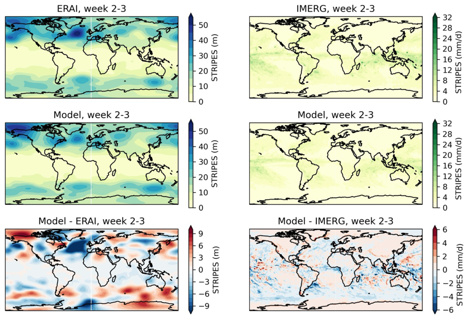
Figure 3 STRIPES index for geopotential height at 500 hPa (left) and precipitation (right) computed using the observations (ERAI and IMERG) and the forecasts (Model) at forecast lead time weeks 2–3. The bottom panels show the difference between the model and the observations.

This index identifies where forecast models capture or miss the regions where the MJO has a significant and predictable impact on the large-scale circulation and precipitation, as well as the strength of the impact. The caveat for the SH is that during boreal winter, MJO teleconnections to this hemisphere are weak.

The STRIPES index depends on the number of MJO events used for its calculation. The shorter the analyzed period, the greater the sensitivity of the index. If users want to compare the STRIPES index computed using two sets of forecasts, the number of MJO events or analyzed periods must be the same for the two sets. Figure 4 shows the STRIPES index computed using two different periods of ERAI: 8 and 18 years, respectively. A comparison of the STRIPES index for the two periods shows that calculation based on the shorter period yields maximum values of the STRIPES index larger than those in the calculation based on a longer period.

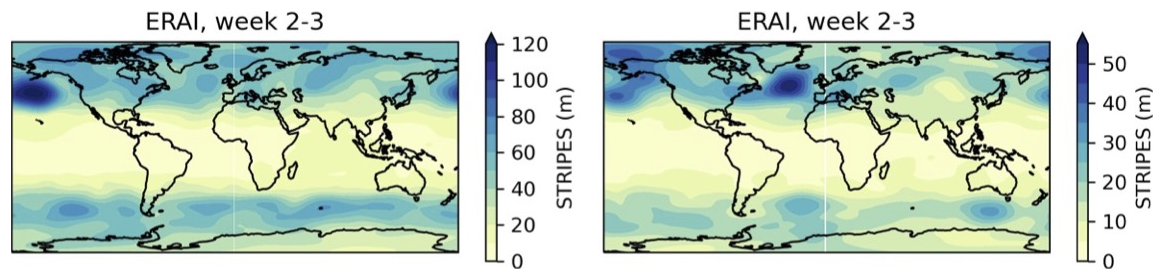
Figure 4 STRIPES index for geopotential height at 500 hPa for weeks 2–3 after MJO events, computed using ERAI for 2011–2018 (left) and 2002–2019 (right).

2.2.2 Pattern correlation and relative amplitude

The two extratropical regions in the NH with the strongest MJO influence are the Pacific North America and the North Atlantic. This can be seen in Fig. 3 and in many other studies (for a complete review, see Stan et al., 2017). These studies also show that MJO teleconnections are not uniform across the MJO phases. The influence on the large-scale Pacific North American (PNA) region is dominated by the MJO convective activity in the tropical Indian Ocean and western Pacific (Mori and Watanabe, 2008), also known as phases 2–3 and 6–7 when using the RMM index. The influence of MJO on the large-scale circulation over the North Atlantic and Eurasia is robust 10–15 d after the occurrence of MJO phase 3 and 7 (Cassou, 2008; Lin et al., 2009).

The ability of the forecast model to capture these relationships can be evaluated using the pattern correlation coefficient (pattern CC) and relative amplitude metrics applied to Z₅₀₀ in each region. The diagnostics for the PNA region are constructed over a domain spanning 20–80° N and 120° E–60° W (Wang et al., 2020) and for the Euro-Atlantic over the area spanning 20–80° N and 60° W–90° E. The pattern CC is calculated between the Z₅₀₀ daily anomalies in the forecasts and those in observations. The relative amplitude is defined as the standard deviation of Z₅₀₀ daily anomalies in the model divided by that in the observations. Figure 5 shows the metrics for the PNA region when MJO events in phases 2–3 and 6–7 are present in the initial conditions of the forecasts. In this example, the prediction of MJO teleconnection pattern is skillful (pattern CC > 0.6) up to two weeks regardless of the MJO phase. In the first week, the amplitude of MJO teleconnection in the forecast data is close to ERAI (relative amplitude ∼ 1). As the lead time increases, the model alternates between underestimating (relative amplitude < 1) and overestimating (relative amplitude > 1) the amplitude of the MJO teleconnections to the PNA region for both MJO phases. At shorter leads (weeks 2–3) the amplitude is largely underestimated following the MJO phases 6–7 whereas at longer leads (weeks 3–4) the overestimation of amplitude is more pronounced for the MJO phases 2–3. Before launching the calculation of the metrics, users have the option to select the computation of composites of Z₅₀₀ daily anomalies over the NH used in the calculation of metrics (Fig. 6). In the window displaying the figures corresponding to pattern CC and relative amplitude, users have the option to download a text file of the values in comma-separated values (csv) format.

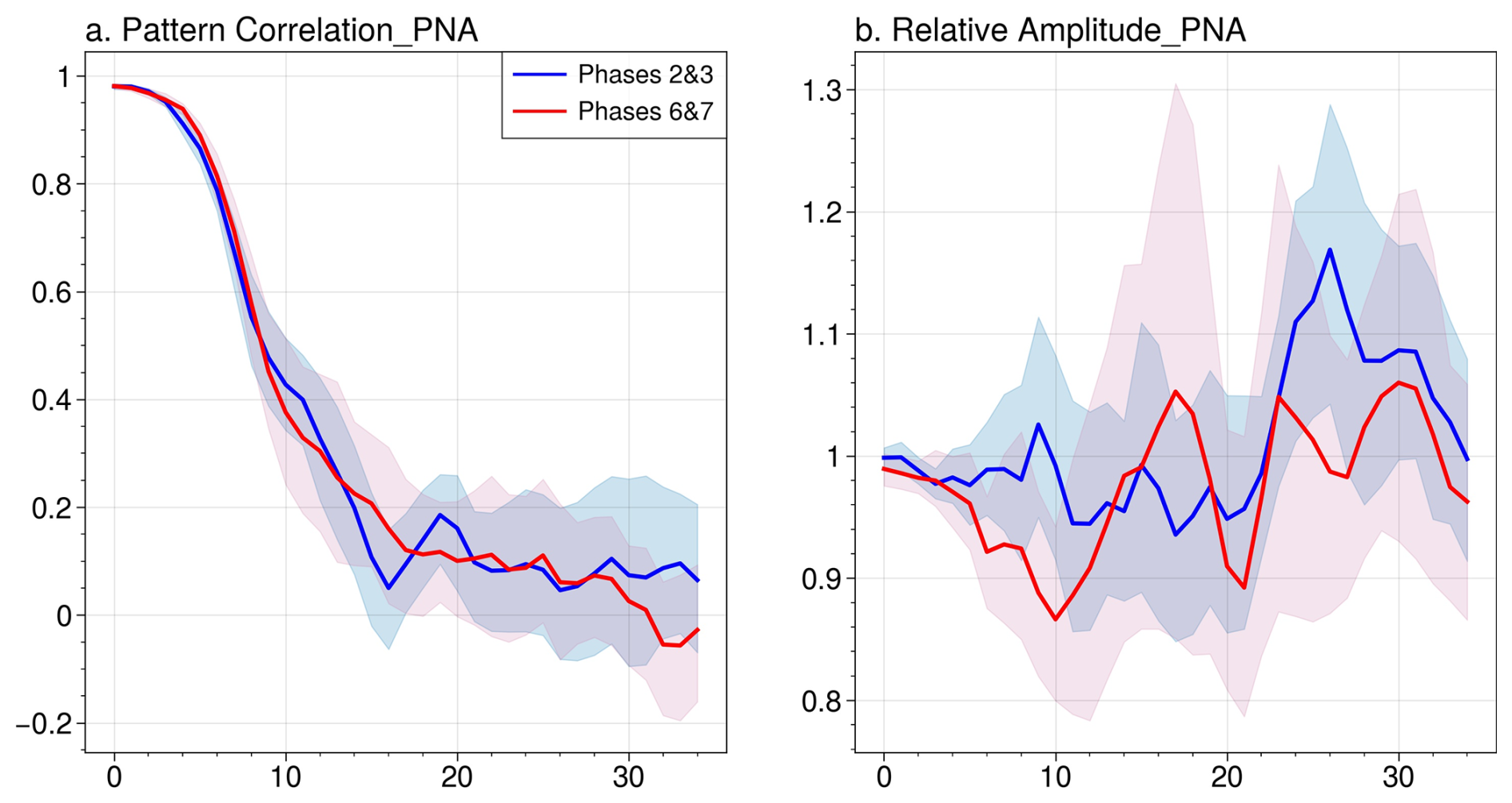
Figure 5 Pattern CC (model vs. observations) and relative amplitude of Z₅₀₀ daily anomalies over the PNA region (20–80° N, 120° E–60° W) as a function of forecast lead days for the MJO phases 2–3 (blue) and 6–7 (red). The shading indicates the 95 % confidence level determined by a bootstrap test with 1000 samples. The lower (upper) boundary represents the 2.5th (97.5th) percentile of the bootstrapping distribution.

Figure 6 shows that in ERAI, the Z₅₀₀ composites after the MJO phases 2–3 resemble the negative PNA pattern, and the composites after the MJO phases 6–7 resemble the positive PNA pattern. The composites based on the forecast data capture the Z₅₀₀ anomaly pattern well in the first two weeks of the forecast after both the MJO phases 2–3 and 6–7, and the accuracy decreases at longer leads. One particular aspect to notice is the model's failure to capture the transition of Z₅₀₀ anomalies associated with the MJO phases 2–3 to the opposite MJO phases (6–7) occurring in week 3 in ERAI. The pattern of the MJO teleconnections in the forecast tends to agree better with ERAI over the North Pacific than over North America, indicating some model deficiencies in predicting the patterns over land rather than over the ocean.

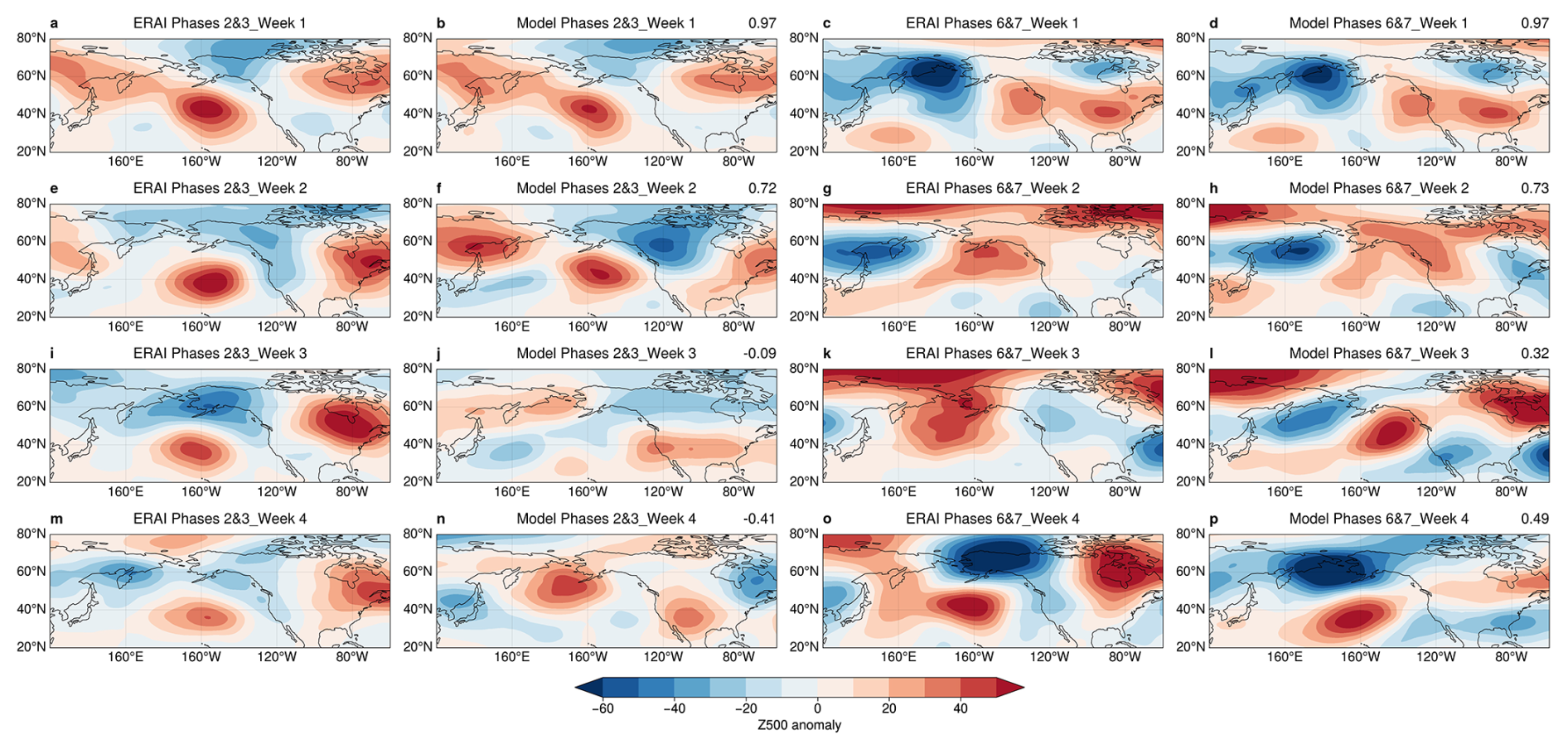
Figure 6 Weekly averaged composites of Z₅₀₀ daily anomalies at lead time week 1 (a–d), week 2 (e–h), week 3 (i–l), and week 4 (m–p) for observations (ERAI) and forecast (model). In the left (right) two columns, forecasts have MJO events in phases 2 and 3 (6 and 7) present in the initial conditions. Numbers in the upper right corners show the pattern CC between model and observations over the PNA region (20–80° N, 120° E–60° W).

These diagnostics help identify model deficiencies related to the pattern and amplitude of specific MJO phase impacts on the large-scale circulation over the PNA and Euro-Atlantic regions.

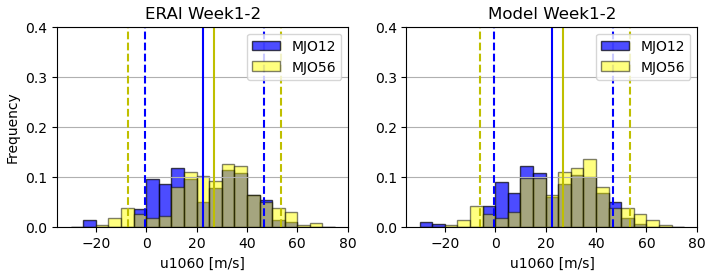
Figure 7 Histograms of daily values of zonal mean zonal wind at 10 hPa 60° N and U1060 from November to March for forecast (Model) and observations (ERAI) for weeks 1–2 following the MJO phases 1–2 (blue) and phases 5–6 (yellow). The solid blue lines indicate the mean values of U1060 during the respective MJO phases. The dashed blue and yellow lines indicate the 5th and 95th percentiles of U1060 during MJO phases 1–2 and 5–6, respectively.

2.2.3 Frequency distribution of zonal wind at 10 hPa

As an initial step in evaluating the stratospheric pathway of teleconnections, this diagnostic is designed to determine the response of the polar vortex to MJO forcing. The polar vortex experiences two opposite extreme conditions: sudden stratospheric warming (SSWs) and strong polar vortex (SPV) events. SSWs occur when dynamic forcings disrupt the stratospheric circulation, resulting in predominantly westward-flowing winds across much of the polar stratosphere. SPVs are associated with strong westerly zonal mean zonal winds caused by anomalously weak planetary wave activity. These extreme events can have impacts that extend to the Earth's surface. The zonal mean zonal wind at 60° N and 10 hPa is used for characterizing the extreme events in the polar vortex (Charlton and Polvani, 2007; Charlton-Perez and Polvani, 2011; Smith et al., 2018; Oehrlein et al., 2020; Baldwin et al., 2021). The diagnostic evaluates the distribution of zonal mean zonal winds at 60° N and 10 hPa averaged over weeks 1–2 and 3–5 after MJO events in phases 1–2 and 5–6 are present in the initial conditions of the forecast (Stan et al., 2022; Garfinkel et al., 2024). Figure 7 shows an example of the zonal mean zonal wind histograms averaged over weeks 1–2 of the forecast.

This diagnostic helps identify the strength of the polar vortex following the MJO activity present in the initial conditions of the forecast. The diagnostic helps assess the influence of the MJO on the stratosphere in models. The stratosphere–troposphere coupling diagnostics following the MJO activity described in the next section provide a deeper analysis of the processes in the model that need to be improved.

2.2.4 Stratosphere–troposphere coupling

The stratosphere–troposphere coupling is evaluated using two diagnostics: (i) the meridionally averaged (40–80° N) meridional heat flux anomaly associated with quasi-stationary planetary waves with wavenumber 1 and 2 at 500 hPa and (ii) the geopotential height anomaly at 100 hPa averaged over the polar cap (55–90° N). Both diagnostics are computed for MJO phases 1–8 and forecast leads week 1 through 5. An enhanced positive heat flux anomaly 2–3 weeks after the MJO in phase 5 is typically associated with the upward propagation of heat fluxes entering the stratosphere, followed by the weakening of the polar vortex. The downward propagation from the stratosphere into the troposphere is shown by the polar cap geopotential height anomaly. Positive polar cap height anomalies in weeks 3–5 following MJO in phase 6 tend to indicate the negative phase of the Northern Annular Mode (NAM) and its downward propagation. Figure 8 shows an example of the stratosphere–troposphere coupling diagnostics.

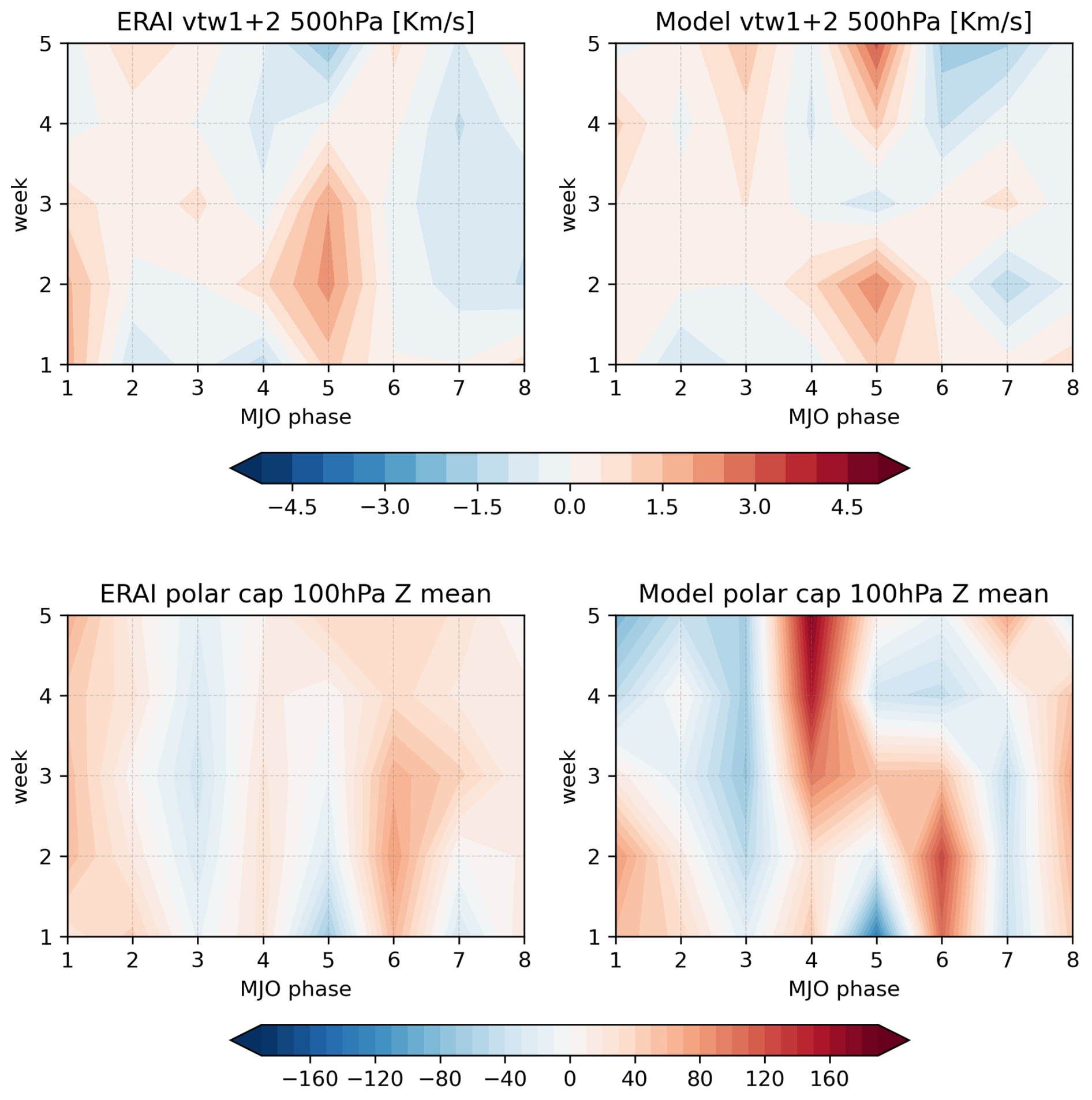
Figure 8 Meridionally averaged heat flux anomalies at 500 hPa (top) and 100 hPa geopotential height anomalies averaged over the polar cap (70–90° N, 0–360) for observations (ERAI) and forecast (model) in weeks 1–5 following MJO phases 1–8 during November–March.

In this case, the model is not able to maintain the strength of the positive heat flux associated with the MJO phase 5 beyond week 2. In fact, the model reverses the sign of the heat flux anomaly at longer forecast leads, suggesting an opposite response of the polar vortex, which is confirmed by the 100 hPa geopotential height anomalies averaged over the polar cap seen in weeks 3–5 following the MJO phase 5.

This diagnostic helps identify the upward troposphere-to-stratosphere coupling using the planetary wave activity flux and the downward stratosphere-to-troposphere coupling using the NAM anomaly following the MJO activity. The diagnostic helps assess the stratospheric pathway of MJO teleconnections.

2.2.5 Extratropical cyclone activity

The package offers two diagnostic tools for evaluating the complex relationship between the MJO and extratropical cyclone activity. One diagnostic computes the composites of eddy kinetic energy (EKE) at 850 hPa for the MJO phases at week 3–4 forecast leads. The EKE is constructed from winds filtered to retain the synoptic-scale variability with periods between 1.2 and 6 d. For this reason, the data required for this diagnostic are recommended to be specified at 6-hourly frequency. The diagnostic can also work with daily mean or 24-hourly data; however, the EKE calculation is sensitive to this aspect, especially if the sample size is relatively short. The calculation of EKE also needs to be done for each ensemble member before calculating the ensemble mean. The composites are computed for the model and a verification dataset, including their statistical significance. Different phases of the MJO are considered because different phases can lead to shifts in preferred storm tracks for extratropical cyclone activity. This can affect the regions that are more likely to experience cyclone activity during specific MJO phases. Certain phases of the MJO are associated with increased intensity of extratropical cyclone activity in specific regions. To measure the agreement between the storm track activity predicted by the model and the verification dataset, the pattern correlation is computed. An example of the composites is shown in Fig. 9. A similar analysis is conducted for Z₅₀₀ to represent the large-scale circulation variability associated with the MJO. The second diagnostic is designed to measure the correspondence between the changes in large-scale circulation induced by MJO and downstream effects that can be more or less favorable for extratropical cyclone formation and intensification. The impact of model errors in the MJO-induced large-scale circulation on the errors in the extratropical cyclone activity can be determined by plotting the pattern correlation of eddy kinetic energy at 850 hPa versus the pattern correlation of Z₅₀₀, for various MJO phases and forecast leads. An example of this diagnostic for the North Atlantic and North Pacific storm track regions is shown in Fig. 10.

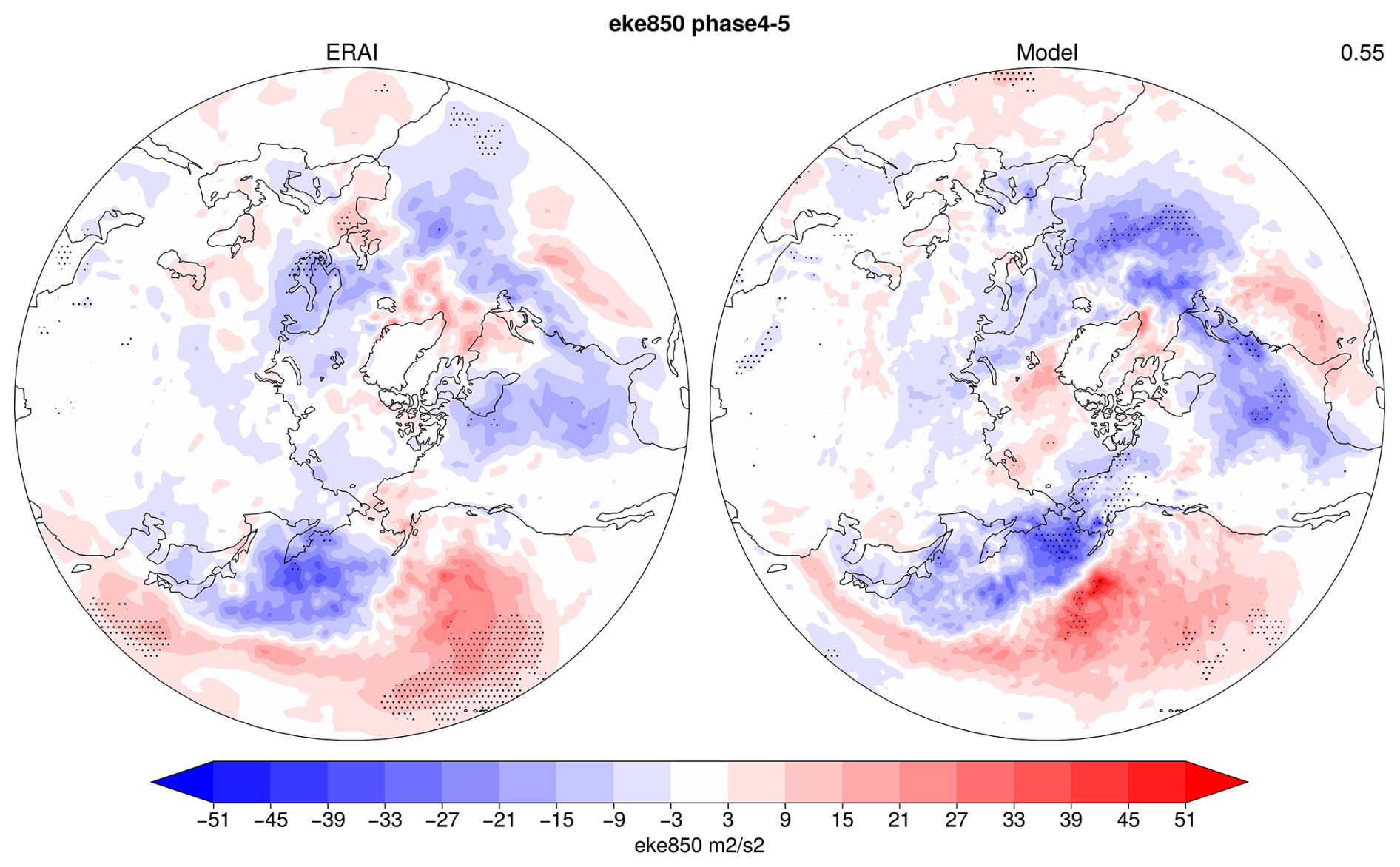
Figure 9 Composites of extratropical cyclone activity (EKE850) during weeks 3– 4 for forecasts with MJO events in phases 4–5 present at the initialization time. Left: reanalysis (ERAI); right: forecast (model). Dotting represents regions where anomalies are statistically significant at the 0.05 level based on a bootstrap resampling calculation. The number in the upper right corner shows the pattern correlation between ERAI and the model over the Northern Hemisphere (20–80° N).

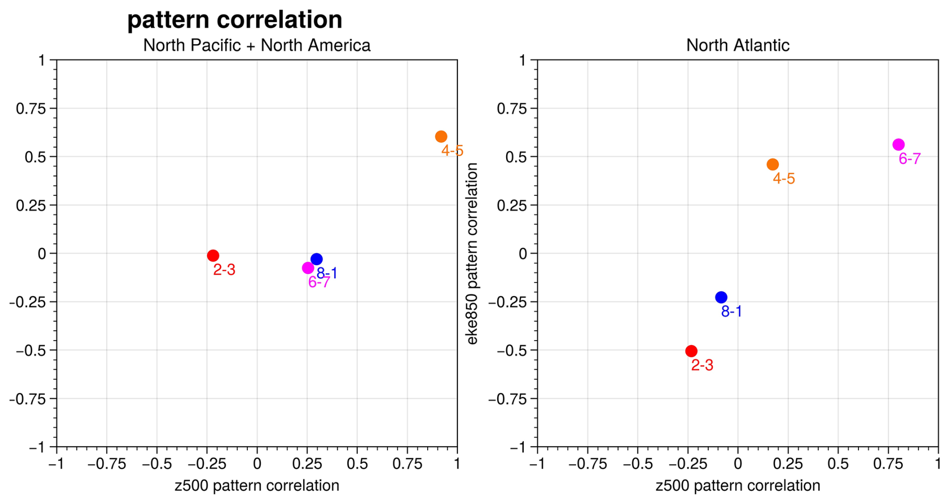
Figure 10 Pattern correlation of week 3–4 composites of EKE850 (y-axis) and Z₅₀₀ (x-axis) between ERAI and model for the North Atlantic (20–80° N, 90° W–30° E) and the North Pacific and North America (20–80° N, 120° E–90° W). Different colors represent different MJO phases.

This diagnostic helps identify model deficiencies in simulating storm track activity modulated by the MJO. The MJO's influence on extratropical cyclones is often associated with synoptic-scale extreme precipitation and temperature events (e.g., Kunkel et al., 2012; Ma and Chang, 2017).

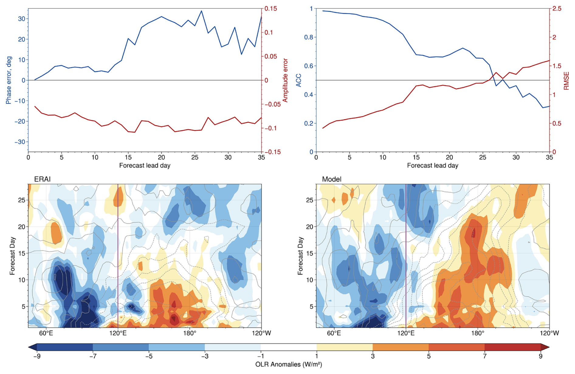
Figure 11 Phase (PERR) and amplitude (AERR) errors (top left), bivariate anomaly correlation (ACC), and root mean square error (RMSE) (top right; the gray solid horizontal line indicates an ACC of 0.5 and an RMSE of 1.25). Longitude–time composites of OLR (W m⁻²; shading) and U850 (contour; interval 0.3 m s⁻¹) anomalies averaged over 15° S–15° N for active MJO events in observations (ERAI) and forecast (model). The results are for events initialized during MJO phases 2 and 3. The vertical lines indicate 120° E (approximately the center of the Maritime Continent). A 5 d moving average is applied.

2.2.6 MJO

Due to the time lag between the MJO activity and the extratropical response, the diagnostics are built using the MJO events present in the initial conditions of the forecasts. However, how the forecast models maintain these events is important for the correct prediction of the MJO teleconnections. For example, the ability of models to maintain the coherence of MJO convection across the Maritime Continent is important for the correct prediction of MJO phases 2 and 3. The propagation speed of MJO events can also influence the MJO teleconnections. For instance, rapidly propagating MJO events result in weak westerlies across the North Atlantic high latitudes (Yadav and Straus, 2017; Yadav et al., 2019). Slowly propagating MJO events can weaken the polar vortex and, downstream, contribute to a relatively stronger impact over the North Atlantic and Eurasia (Yadav et al., 2024). The diagnostics package calculates the RMM1 and RMM2 indices following the method in Gottschalk et al. (2010) using U₈₅₀ and U₂₀₀ from ERAI and NOAA OLR (Liebman and Smith, 1996). These are then used to compute the bivariate anomaly correlation (ACC), root mean square error (RMSE), and amplitude (AERR) and phase error (PERR) between the forecast and observations. The eastward propagation of the MJO pattern is evaluated using Hovmöller diagrams of the daily anomalies for OLR and zonal wind at 850 hPa averaged over 15° S–15° N for active MJO events in the initial conditions of the forecast. Examples of these metrics are shown in Fig. 11. The definitions of ACC, RMSE, AERR, and PERR are adopted from Rashid et al. (2011):

$$\begin{array}{}\text{(1)}& \begin{array}{rl}& \mathrm{ACC}\left(\mathit{\tau }\right)=\\ & {\displaystyle \frac{\sum _{t=\mathrm{1}}^N\left[a_{\mathrm{1}}\left(t\right)b_{\mathrm{1}}(t,\mathit{\tau })+a_{\mathrm{2}}\left(t\right)b_{\mathrm{2}}(t,\mathit{\tau })\right]}{\sqrt{\sum _{t=\mathrm{1}}^N\left[a_{\mathrm{1}}(t{)}^{\mathrm{2}}+a_{\mathrm{2}}(t{)}^{\mathrm{2}}\right]}\sqrt{\sum _{t=\mathrm{1}}^N\left[b_{\mathrm{1}}(t,\mathit{\tau }{)}^{\mathrm{2}}+b_{\mathrm{2}}(t,\mathit{\tau }{)}^{\mathrm{2}}\right]}}}\end{array}\end{array}$$

$$\begin{array}{}\text{(2)}& {\displaystyle }\begin{array}{rl}& \mathrm{RMSE}\left(\mathit{\tau }\right)=\\ & \sqrt{{\displaystyle \frac{\mathrm{1}}{N}}\sum _{t=\mathrm{1}}^N\left({\left[a_{\mathrm{1}}\left(t\right)-b_{\mathrm{1}}(t,\mathit{\tau })\right]}^{\mathrm{2}}+{\left[a_{\mathrm{2}}\left(t\right)-b_{\mathrm{2}}(t,\mathit{\tau })\right]}^{\mathrm{2}}\right)}\end{array}\text{(3)}& {\displaystyle }\begin{array}{rl}\mathrm{AERR}\left(\mathit{\tau }\right)& ={\displaystyle \frac{\mathrm{1}}{N}}\sum _{t=\mathrm{1}}^N\left(\sqrt{b_{\mathrm{1}}(t,\mathit{\tau }{)}^{\mathrm{2}}+b_{\mathrm{2}}(t,\mathit{\tau }{)}^{\mathrm{2}}}\right.\\ & \left.-\sqrt{a_{\mathrm{1}}(t{)}^{\mathrm{2}}+a_{\mathrm{2}}(t{)}^{\mathrm{2}}}\right)\end{array}\text{(4)}& {\displaystyle }\begin{array}{rl}\mathrm{PERR}\left(\mathit{\tau }\right)=& {\displaystyle \frac{\mathrm{1}}{N}}\sum _{t=\mathrm{1}}^N{\tan }^{-\mathrm{1}}\\ & \left({\displaystyle \frac{a_{\mathrm{1}}\left(t\right)b_{\mathrm{2}}(t,\mathit{\tau })-a_{\mathrm{2}}\left(t\right)b_{\mathrm{1}}(t,\mathit{\tau })}{a_{\mathrm{1}}\left(t\right)b_{\mathrm{1}}(t,\mathit{\tau })+a_{\mathrm{2}}\left(t\right)b_{\mathrm{2}}(t,\mathit{\tau })}}\right)\end{array}\end{array}$$

where a₁ and a₂ are RMM1 and RMM2 in observations, b₁ and b₂ are RMM1 and RMM2 in forecast data, t denotes the initialization time with a lead time of τ days, and N is the total number of predictions. As noted by Rashid et al. (2011), this is not equivalent to the difference between an average phase of the forecasts and observations, and positive PERR values indicate that the MJO in the forecasts leads the event in observations.

The AERR and PERR metrics show that the model predicts MJO events with weaker amplitude and faster phase speed than in ERAI. The ACC shows that the forecast skill drops below 0.5 after ∼27 d at about the same time when RMSE = 1.4. The Hovmöller diagram shows that in the model convective activity takes a longer time to propagate across the Maritime Continent.

This diagnostic helps identify the errors in the amplitude, phase speed of the MJO as predicted by the model. It also shows the model's ability to predict the propagation of the MJO across the Maritime Continent and the coupling between the circulation and convective activity associated with MJO events.

2.2.7 Surface air temperature

The impact of the MJO on the surface air temperature is evaluated in the composites of T2m anomalies for forecasts that have MJO events in phases 3 and 7 present in the initial conditions. The phases are chosen because they are known to have the strongest teleconnections to temperature patterns in the NH. Composite maps are constructed for forecast leads ranging from week 1 to week 5 and the observed counterparts. The composite maps are displayed as stereographic projections of the NH and include statistical significance. To quantify the accuracy of the forecasts, the pattern correlation between the forecast data and the verification data are computed for each composite map. This metric provides a measure of how well the pattern of predicted T2m matches the observed patterns. Because of the typical 15 d time lag between MJO activity and observed temperature changes in the NH, the first two weeks provide information on model errors due to local processes affecting the temperature anomaly patterns. If the MJO diagnostic indicates a slower (faster) propagation of the MJO than in observations, the errors in the T2m pattern can also be attributed to the timing of the MJO impact on the existing temperature anomalies. The strength of the MJO events (e.g., measured by the relative amplitude diagnostic) can also affect the length of the lag and the effect of MJO teleconnection to the region. Figure 12 shows an example of T2m composites in week 3 after MJO events in phase 3 are present in the initial conditions of the forecasts.

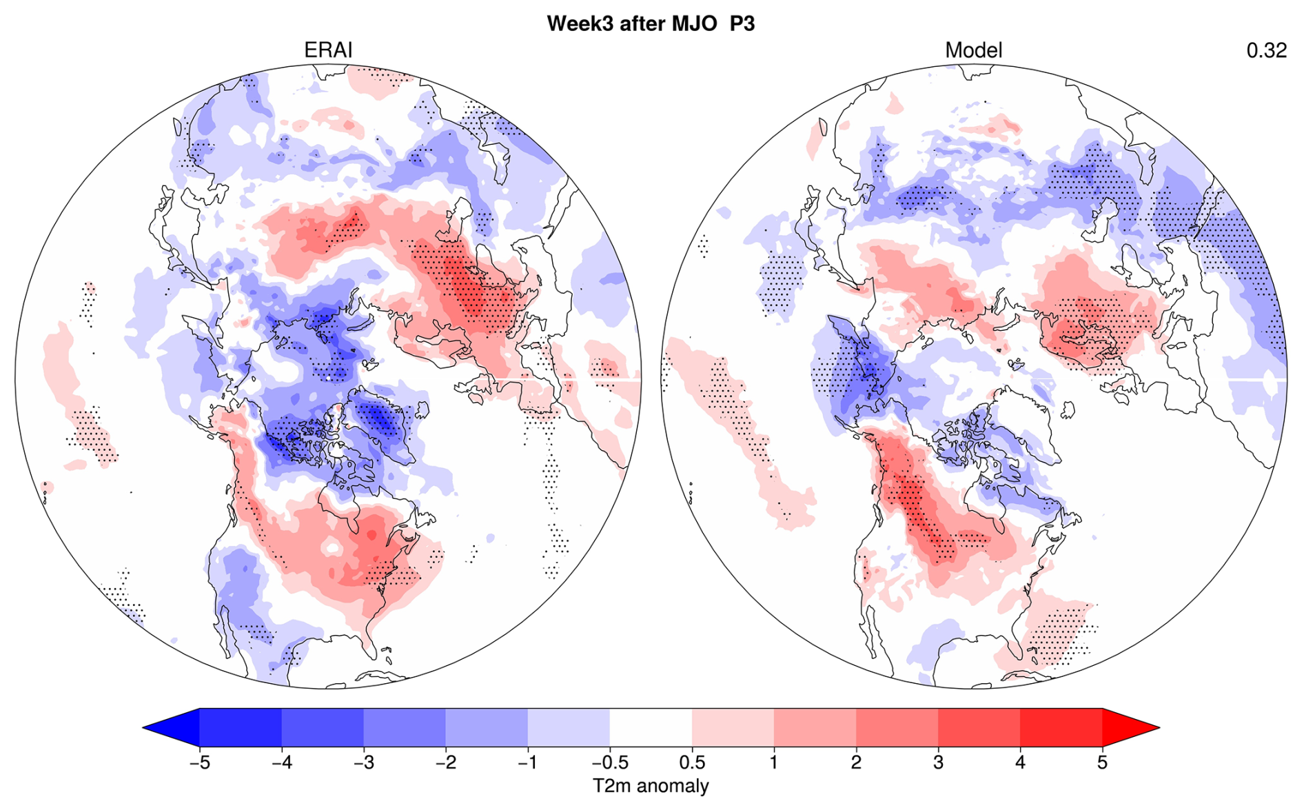
Figure 12 Composites of T2m daily anomalies in November–March for observations (ERAI) and forecast (model) for week 3 following the MJO phase 3. Dotted regions indicate statistical significance. The number in the upper right corner represents the pattern correlation between the two maps.

The model deficiencies are reflected by the weak anomaly correlation (0.32) between the model and ERAI. Regionally, the model misses the center of positive anomalies along the east coast of North America and Eurasia and the center of negative temperature anomalies over the North Pole.

This diagnostic helps identify whether the forecast captures the specific temperature anomaly patterns in different regions of the NH, whether the model predicts the sign reversal of T2m anomalies seen in observations for the opposite MJO phases, and the strength of the MJO impact on the surface air temperature.

3 Summary, limitations, and future development

The MJO teleconnections diagnostics package is a Python tool that provides process-level evaluation of the MJO and its teleconnections predicted by forecast models. The package is driven by a GUI that facilitates the handling of large and complex datasets that are typically generated by forecast systems. The evaluation has the flexibility to be conducted using an included dataset or user-specified datasets. The diagnostics included in the package have been applied to peer-reviewed studies, and the calculations are consistent with previous results. The list of diagnostics, in the order they appear on the GUI, includes:

• The STRIPES index for geopotential height at 500 hPa identifies regions where forecast systems capture/miss the impact of MJO across all its phases on the extratropics large-scale circulation of the northern and southern hemispheres during boreal winter.

• The STRIPES index for precipitation identifies regions where extratropical precipitation in the forecast data are influenced or not by the MJO events present in the initial conditions of the forecasts during boreal winter.

• The pattern CC and relative amplitude for the PNA region (20–80° N, 120° E–60° W) measure the forecast skill (pattern correlation) of the MJO teleconnections over the PNA region following the MJO convective activity located over the central Indian Ocean and eastern Maritime Continent (phases 2–3) and western central Pacific and central Pacific (phases 6–7). The relative amplitude provides a quantitative measure of the amplitude of the response in the forecast relative to verification.

• The pattern CC and relative amplitude for the Euro-Atlantic sector (20–80° N, 60° W–90° E) provide the same information as the diagnostics for the PNA region except for the Euro-Atlantic sector.

• The stratospheric pathway identifies model deficiencies in forecasting the stratosphere–troposphere coupling mechanism driving the MJO teleconnections following the stratospheric pathway. The diagnostics evaluate the amplitude of the meridionally averaged meridional heat flux in the middle troposphere (500 hPa) for the upward leg (weeks 2–3) and the downward leg of the coupling (weeks 4–5) as well as the response of the polar vortex measured by the 100 hPa geopotential height.

• The histogram of 10 hPa zonal wind provides information on the forecast system's ability to predict the climatological distribution of the polar vortex winds. This diagnostic is a good indicator of the model limitations caused by the number of vertical levels and model top as models with a low top struggle to tap into the source of predictability arising from the stratospheric pathway (Stan et al., 2022).

• The MJO diagnostic provides the model skill in predicting the MJO amplitude and phase speed. The Hovmöller diagram of OLR and zonal wind at 850 hPa after MJO events in phases 2–3 are present in the initial condition of forecasts provides an estimation of the model's ability to predict the propagation of MJO activity across the Maritime Continent.

• The composites of T2m after MJO events in phases 3 and 4 present in the initial conditions of forecasts provide information on the model's ability to tap into the source of predictability associated with the MJO.

The modular structure of the diagnostics allows for future expansion of the codebase to compute other diagnostics. For example, diagnostics for the evaluation of biases in the models' mean state would provide a complete picture for the model evaluation. Other diagnostics such as the wave activity flux (WAF; Plumb, 1985; Takaya and Nakamura, 2001) and the stationary wavenumber on the Mercator projection (Hoskins and Ambrizzi, 1993) are sometimes used to evaluate the Rossby wave propagation and the Rossby waveguides. These diagnostics will provide information on the model's ability to predict the generation of Rossby waves with the observed propagation characteristics and model ability to predict unbiased mean states in the subtropics (e.g., subtropical westerly jet).

Further improvements in the regridding algorithm are warranted to reduce the calculation run time. The package could also be improved to allow direct model to model comparison when possible.

Appendix A: Data pre-processing

Table A1 Variables accepted by the package for forecast data. The time variable must have units of days since the starting date of the forecast.

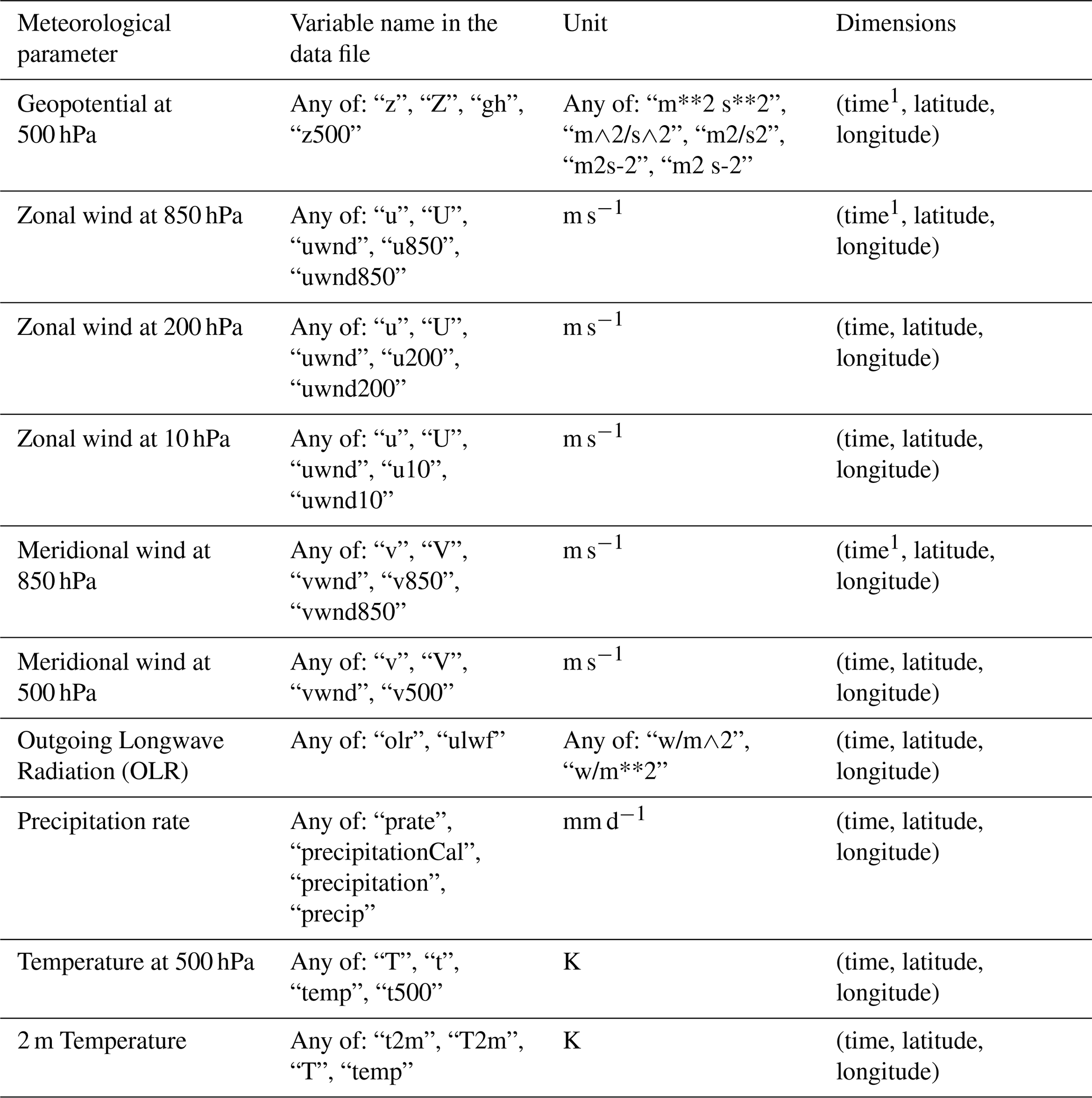
¹ The extratropical cyclone activity diagnostics recommend using 6-hourly data. For those fields, time should be replaced by forecast_hour.