Implementation of solar UV and energetic particle precipitation within the LINOZ scheme in ICON-ART

We extended the Linearized ozone scheme – LINOZ in the ICON (ICOsahedral Nonhydrostatic) – ART (the extension for Aerosols and Reactive Trace gases) model system to include NO_y formed by auroral and medium-energy electrons in the upper mesosphere and lower thermosphere, and the corresponding ozone loss, as well as changes in the rate of ozone formation due to the variability of the solar radiation in the ultraviolet wavelength range. This extension allows us to realistically represent variable solar and geomagnetic forcing in the middle atmosphere using a very simple ozone scheme. The LINOZ scheme is computationally very cheap compared to a full middle atmosphere chemistry scheme, yet provides realistic ozone fields consistent with the stratospheric circulation and temperatures, and can thus be used in climate models instead of prescribed ozone climatologies. To include the reactive nitrogen (NO_y) produced by auroral and radiation belt electron precipitation in the upper mesosphere and lower thermosphere during polar winter, the so-called energetic particle precipitation indirect effect, an upper boundary condition for NO_y has been implemented into the simplified parameterization scheme of the N₂O/NO_y reactions. This parameterization, which uses the geomagnetic A_p index, is also recommended for chemistry-climate models in the CMIP6 experiments. With this extension, the model simulates realistic “tongues” of NO_y propagating downward in polar witner from the model top in the upper mesosphere into the mid-stratosphere with an amplitude that is modulated by geomagnetic activity. We then expanded the simplified ozone description used in the model by applying LINOZ version 3. The additional ozone tendency from NO_y is included by applying the corresponding terms of the version 3 of LINOZ. This NO_y, coupled as an additional term in the linearized ozone chemistry, led to significant ozone losses in the polar upper stratosphere in both hemispheres which is qualitatively in good agreement with ozone observations and model simulations with EPP-NO_y and full stratospheric chemistry. In a subsequent step, the tabulated coefficients forming the basis of the LINOZ scheme were provided separately for solar maximum and solar minimum conditions. These coefficients were then interpolated to ICON-ART using the F10.7 index as a proxy for daily solar spectra (UV) variability to account for solar UV forcing. This solar UV forcing in the model led to changes in ozone in the tropical and mid-latitude stratosphere consistent with observed solar signals in stratospheric ozone.

1 Introduction

The solar influence in the middle atmosphere involves various contributors, including the ozone response triggered by both energetic particle precipitation (EPP) and ultraviolet (UV) solar radiation (Gray et al., 2010; Matthes et al., 2017; Dhomse et al., 2022; Maycock et al., 2016). Energetic particles precipitate into the atmosphere from multiple sources: solar protons, accelerated to energies of a few hundred MeV, are associated with huge eruptions of the solar corona; galactic cosmic rays (GCRs), which include particles with energies ranging from hundreds of MeV up to GeV (Anchordoqui et al., 2003; Thoudam et al., 2016); Auroral electrons, precipitated during magnetic reconnection in the magnetotail, having energies ranging from a few keV up to hundreds of keV; and radiation belt electrons, containing energies up to several MeV during geomagnetic storms (Giovanni, 2020; Sinnhuber et al., 2012). The precipitation of energetic particles into the middle atmosphere contributes to the formation of a chain of ionic reactions by ionizing and dissociating species such as N₂ and O₂, producing neutral reactive radicals such as H, OH, N, and NO (Sinnhuber et al., 2012). Both HO_x (H, HO₂) and NO_x (N, NO, NO₂) trigger catalytic chemical cycles associated with the mesospheric and stratospheric ozone loss (Lary, 1997; Sinnhuber et al., 2012). HO_x has a shorter atmospheric lifetime compared to NO_x and exhibits a higher potential for inducing ozone loss in the mesosphere (Bates and Nicolet, 1950; Nicolet, 1975; Lary, 1997). In contrast, NO_x is longer-lived and can be transported downward through the stratosphere, leading to ozone loss in the stratosphere, particularly during polar winter and spring (Rozanov et al., 2012; Randall et al., 2006).

Electron precipitation from the magnetosphere – from the auroral and radiation belt regions – occurs nearly continuously, much more frequent than solar proton events. These particles do not penetrate as deeply into the middle atmosphere to the lower stratosphere as high-energy solar protons associated with solar proton events do, yet they can still produce larger amounts of NO_x and are the main source for NO_x in the high-latitude upper mesosphere and lower thermosphere (Sinnhuber et al., 2012). NO_x variations in the mesosphere and lower thermosphere due to geomagnetic activity can be considered a proxy for electron precipitation (Kirkwood et al., 2015; Hendrickx et al., 2015; Sinnhuber et al., 2012, 2016; Barth et al., 2002).

The distinction between the direct and indirect effects of EPP arises from where NO_x is produced and its subsequent impact on ozone. When NO_x is produced in the mesosphere or lower thermosphere, it does not immediately affect stratospheric ozone. Instead, it is transported downward into the stratosphere within the polar vortex before causing ozone depletion, a process known as the EPP indirect effect (EPP IE) (Randall et al., 2006; Seppälä et al., 2014). In contrast, NO_x produced in the lower mesosphere or stratosphere can cause ozone depletion directly in those regions. Although both processes ultimately involve ozone loss via NO_x, we use the established terms “direct effect” and “indirect effect” to reflect their distinct pathways and to align with common usage in the literature. A recent publication by Seppälä et al. (2025) indicates that a direct effect on atmospheric dynamics via mesospheric HO_x production and ozone loss by precipitating magnetospheric electrons in early winter might be possible as well.

As ozone plays an important role in radiative heating in the middle atmosphere, a realistic ozone field is essential in order to obtain a reasonable description of dynamical processes (Braesicke and Pyle, 2003, 2004). Despite numerous studies on the impact of solar forcing on the climate system through the top-down effect, conclusive results have yet to be reached. The main reason is the limited statistics that can be obtained with resource-demanding full chemistry climate models. For such studies, a fast but realistic ozone scheme is essential to achieve a sufficient number of realizations.

The ozone loss in the stratosphere, induced by the downward transport of NO_x during polar winter and spring, can lead to net radiative cooling due to the reduction in UV absorption. Conversely, during the polar night, ozone loss results in net radiative heating because of the reduction in IR emission (Sinnhuber et al., 2018). These changes subsequently alter the dynamics of the middle atmosphere, initiating a chain of dynamical shifts that contribute to top-down solar forcing during polar winter and spring. This process, driven by the EPP-NO_x indirect effect, appears to impact tropospheric weather systems in the high and mid-latitudes during winter and spring (Seppälä et al., 2009; Maliniemi et al., 2014; Rozanov et al., 2012; Matthes et al., 2017).

Variable solar UV is another source of ozone variability in the stratosphere (Gray et al., 2010; Matthes et al., 2017; Dhomse et al., 2022; Maycock et al., 2016). Ozone formation is driven by photolysis of O₂ in the UV spectral range at wavelengths less than 220 nm, and changes in the UV flux will affect the rate of formation of ozone particularly around the tropical stratopause (Gray et al., 2010; Matthes et al., 2017). The variations of solar ultraviolet radiation depend on sunspot activity that occurs in 11-year solar cycles. During solar maximum, increased levels of UV radiation lead to higher rates of oxygen photolysis, resulting in the production of ozone (Dhomse et al., 2022; Maycock et al., 2016).

The changes in radiative heating rates induced by both direct modulation of UV radiation at the tropical stratopause and indirect modulation through ozone changes alter temperatures and dynamics of the middle atmosphere (Gray et al., 2010; Matthes et al., 2017). These radiative heating changes alter the meridional temperature gradient (Holton, 2004), thereby affecting the zonal wind. As a result, the changes in the zonal wind can modulate the behavior of planetary waves, penetrating further down to the earth's surface, eventually impacting the lower atmospheric circulation patterns such as the Arctic Oscillation (AO) and the North Atlantic Oscillation (NAO) (Gray et al., 2010; Matthes et al., 2017; Kodera and Kuroda, 2002).

In this paper, we describe the implementation of variable solar UV radiation and particle precipitation by applying the UBC-NO_y in the simplified NO_y scheme and using the NO_y tendency term in the linearized ozone chemistry scheme LINOZ. This scheme is incorporated into the chemistry-climate model ICON-ART, and the impact of solar variability due to EPP and changes in solar UV radiation on ozone in the middle atmosphere is assessed using ICON-ART-LINOZ. The results are compared with observations of NO_y from the Michelson Interferometer for Passive Atmospheric Sounding (MIPAS) (Fischer et al., 2008), as well as with model outputs from the ECHAM/MESSy Atmospheric Chemistry (EMAC) model (Jöckel et al., 2010), as shown in Funke et al. (2014a) and Sinnhuber et al. (2018). Additionally, the solar signal in stratospheric ozone derived from satellite data is compared, as shown in Maycock et al. (2016).

Several previous parameterizations have been developed to simulate transient ozone in chemistry-climate models. The scheme introduced by Cariolle and Teyssedre (2007) provides a linear parameterization of ozone photochemistry, including a representation of polar ozone loss, which we also adopt in our setup. Another example is the SWIFT scheme discussed by Wohltmann et al. (2017) and Kreyling et al. (2018), which uses an efficient approach based on a fourth-order polynomial fit to full chemistry simulations. Although SWIFT offers high accuracy and speed, it was originally designed for use with Lagrangian transport models, making it less directly applicable to our ICON setup. In this study, we used the LINOZ scheme, which provides a computationally efficient and dynamically consistent alternative suitable for integration into global models that require interactive, yet fast ozone chemistry.

The ICON-ART-LINOZ scheme is capable, in principle, of simulating ozone under changing greenhouse gas (GHG) conditions. In the full LINOZ V3 framework, N₂O and CH₄ can be prescribed from evolving boundary conditions, allowing their long-term trends to influence stratospheric ozone through interactive chemistry (Hsu and Prather, 2010). However, in our current implementation, N₂O and CH₄ are treated as fixed climatological fields and thus do not vary with changing GHG scenarios. If future studies require simulations under substantially different climate conditions or trace gas abundances, the LINOZ tables can be regenerated around a new reference state to maintain accuracy in the ozone response. This flexibility makes ICON-ART-LINOZ suitable for exploring ozone–climate interactions in future scenarios, provided that the relevant chemical inputs are updated accordingly.

The LINOZ parameterization has been shown to perform well in extreme climate scenarios, such as the CMIP 4 × CO₂ case discussed by Meraner et al. (2020). In their study, both the Cariolle and LINOZ V1 schemes produced reasonable ozone responses to substantial temperature increases. Our implementation of LINOZ V3 (Hsu and Prather, 2010) builds on this by addressing a key limitation identified by Meraner et al. (2020) which is the absence of Quasi-Biennial Oscillation-related feedback on NO_y due to vertical transport in LINOZ V1. In LINOZ V3, this coupling is included, allowing for a more realistic simulation of the variability of ozone and NO_y, particularly in the tropical stratosphere above 10 hPa. This confirms that the ICON-ART-LINOZ system even in its current O₃–NO_y-only configuration, remains applicable to study ozone in high CO₂ scenarios, particularly where NO_y-driven chemistry and temperature-dependent processes dominate.

The description of the ICON-ART model can be found in Sect. 2.1 and 2.2, and the LINOZ is discussed in Sect. 2.3. The experimental setup is described in Sect. 3. Model developments including the upper boundary condition of NO_y (UBC-NO_y), the inclusion of the NO_y-based tendency term, and the incorporation of solar UV variability, detailed in Sect. 4.1–4.3. The quantification of the EPP and UV impact on ozone and evaluation against MIPAS observations and the EMAC model is discussed in Sect. 5.1 and 5.2.

2 The ICON-ART model

2.1 The ICON model description

ICON stands for ICOsahedral Nonhydrostatic model system and has been designed by a joint development between the German Weather Service (DWD), the Max Planck Institute for Meteorology (MPI-M), Deutsches Klimarechenzentrum (DKRZ), the Karlsruhe Institute of Technology (KIT), and the Center for Climate Systems Modeling (C2SM) as a unified version of numerical weather prediction (NWP) and climate configuration (Zängl et al., 2015, 2022; Jungclaus et al., 2022). Our study relies on ICON (NWP) physics package.

The horizontal discretization in ICON is based on an unstructured icosahedral-triangular C grid (Staniforth and Thuburn, 2012) and It uses a hybrid vertical coordinate system that is terrain-following near the surface and transitions to constant height levels in the upper levels (Zängl et al., 2022; Leuenberger et al., 2010). Employing icosahedral-triangular C grid type is advantageous for simulating polar regions, as it eliminates the singularity issue that would otherwise be encountered when applying latitude-longitude grids (Staniforth and Thuburn, 2012).

In the ICON model, physical processes are considered by parameterization schemes that are distinct from the dynamical core which solves the governing equations of atmospheric motion. The NWP physics package, as detailed by (Zängl et al., 2015) consists of parameterizations for radiative transfer, cloud microphysics, convection, turbulent diffusion, and surface interactions. These schemes are specifically optimized for numerical weather prediction applications, which differs from the ECHAM6-based approaches used in climate modeling (Stevens et al., 2013; Jungclaus et al., 2022). The ICON physics–dynamics coupling scheme distinguishes between fast processes, such as saturation adjustment and turbulence, which are calculated with shorter time steps, and slower processes, such as radiation and convection, which are computed at longer intervals (Zängl et al., 2015, 2022).

2.2 Chemistry and transport in ICON-ART

The extension for Aerosols and Reactive Trace Gases (ART) developed at the Karlsruhe Institute of Technology (KIT) enables the inclusion of aerosols and atmospheric chemistry into ICON (Rieger et al., 2015). The ART model extension can be incorporated into ICON for numerical weather prediction (NWP) (Rieger et al., 2015) as well as climate configuration (Schröter et al., 2018). Trace gases are included in ICON-ART with the ART coupler without changing the original ICON code. This setup allows for a flexible description of atmospheric trace gases using meta information within XML files, enabling a variety of simulations with different complexities (Schröter et al., 2018; Weimer, 2019). ICON-ART tracers are then transported by the ICON wind fields, and can interact with the radiative heating in ICON.

2.2.1 Transport of trace gases

Trace gases in ICON-ART are transported using the same nonhydrostatic dynamical core as the rest of the model, applying a finite-volume approach on an icosahedral grid (Zängl et al., 2015). Advection of tracers is taken into account using a flux-form semi-Lagrangian method, which is mass conserving and suitable for global-scale simulations (Rieger et al., 2020). In addition to advective transport, ICON-ART accounts for vertical diffusion in the planetary boundary layer, where turbulent mixing is parameterized following the prognostic turbulence kinetic energy (TKE) scheme developed by Raschendorfer (2001).

2.2.2 Photolysis rates

Photolysis rates in ICON-ART are handled differently depending on the chemistry scheme used:

• LINOZ: this scheme uses precomputed photolysis rates stored in tabulated form, calculated using the PRATMO (Prather's Atmospheric Model) code (Hsu and Prather, 2010). These rates cover the stratosphere (10–60 km) include Rayleigh scattering, and are calculated with a fixed albedo of 0.30 to account for average cloud cover. LINOZ does not calculate photolysis rates interactively; it uses these precomputed values for efficiency. It is important to note that LINOZ does not account for $J_{{\mathrm{O}}_{\mathrm{2}}}$ photolysis above 60 km, and Lyman-alpha photolysis of $J_{{\mathrm{H}}_{\mathrm{2}}\mathrm{O}}$ is not included below 70 km, where its impact is minimal.

• MECCA: the full chemistry scheme (MECCA) calculates photolysis rates using CloudJ7.3 (Prather, 2015), a module that provides accurate photolysis rates based on the solar zenith angle, cloud cover, and atmospheric composition. This module is configurable and allows for accurate photolysis calculations across various atmospheric layers.

2.2.3 Chemistry schemes

ICON-ART supports three chemistry approaches:

• Simple Lifetime Mechanism: for tracers with a fixed e-fold decay time, providing computational efficiency without complex chemical interactions (Rieger et al., 2015).

• LINOZ: a linearized ozone chemistry scheme (McLinden et al., 2000; Hsu and Prather, 2010), optimized for the stratosphere, where solar UV and EPP impact ozone.

• MECCA: a comprehensive full chemistry scheme (Sander et al., 2011), with numerical integration managed using the Kinetic PreProcessor (KPP) (Sandu and Sander, 2006), generating Fortran90 code for solving the differential equations of the chemical mechanism. The Rosenbrock solver of the third order (Sandu et al., 1997) is used for numerical stability. For the MECCA scheme, species can be calculated individually or conceptually grouped (e.g., NO_y, HO_y) in order to simplify chemical interactions. However, this is not automatic. Instead, each species is calculated individually, unless explicitly defined as a group in the chemical mechanism (Sander et al., 2011). A specific example of this is the “generic RO₂” approach in MECCA, where multiple organic peroxy radicals are shown by a single generic RO₂ species, reducing computational cost while maintaining chemical accuracy. The MECCA setup in ICON-ART is configured using an XML file, allowing users to define or extend chemical mechanisms without modifying the model code (Schröter et al., 2018).

2.3 The linearized ozone scheme (LINOZ) as included in ART

For a more realistic description of ozone fields compared to a prescribed ozone climatology, we have relied on a linearized ozone scheme, LINOZ (McLinden et al., 2000). LINOZ provides a computationally efficient alternative to a full middle atmosphere chemistry scheme, while still generating ozone fields that align well with stratospheric circulation and temperatures.

In this study, we adapted the LINOZ V3 model from Hsu and Prather (2010) to focus on the interactions between NO_y and O₃ under solar variable forcing. NO_y is calculated following the LINOZ V3 formulation, which includes photochemical production based on fixed N₂O, stratospheric and mesospheric losses, a tropospheric sink (Olsen et al., 2001; Hsu and Prather, 2010), and an upper boundary condition (UBC) that incorporates EPP-NO_y input.

We employ an O₃–NO_y-only version of LINOZ V3. The net chemical tendency for each species is represented as a first-order Taylor expansion around climatological mean states. The production (P) and loss (L) terms are computed using precomputed coefficients that describe the sensitivity of chemical rates to the concentrations of relevant species, temperature (T), and the overhead ozone column (CO₃). These coefficients are derived from the PRATMO photochemical box model (Prather, 1992; Prather and Jaffe, 1990; Hsu and Prather, 2010), which simulates stratospheric chemistry involving O₃, NO_y, N₂O, CH₄, and H₂O.

In our O₃–NO_y-only setup, these coefficients are simplified to capture only interactions between O₃ and NO_y, while N₂O, CH₄, and H₂O are treated as fixed climatological fields. Thus, only O₃ and NO_y are dynamically calculated in the LINOZ scheme, whereas other species are treated as fixed climatological fields. This method ensures efficient computation and successfully captures key ozone–NO_y interactions relevant to our study, while processes involving dynamically varying N₂O lie outside the scope of the current implementation.

The coefficients for the production and loss terms are precomputed for 25 pressure levels (∼10–58 km), 18 latitudes, and 12 months. These values are stored in lookup tables and used to efficiently calculate the chemical tendencies for O₃ and NO_y during model integration.

The differential equation representing the linearized ozone version 3 method follows Hsu and Prather (2010):

$$\begin{array}{}\text{(1)}& \begin{array}{rl}{\displaystyle \frac{\mathrm{d}{f}_i}{\mathrm{d}t}}& =(P-L{)}_i^{{\mathrm{0}}_i}+\sum _{j=\mathrm{1}}^{j=\mathrm{5}}{\displaystyle \frac{\partial (P\mathrm{-}L{)}_i}{\partial f_j}}{|}_{\mathrm{0}}\left(f_j-f_j^{\mathrm{0}}\right)\\ & +{\displaystyle \frac{\partial (P\mathrm{-}L{)}_i}{\partial T}}{|}_{\mathrm{0}}\left(T-T^{\mathrm{0}}\right)+{\displaystyle \frac{\partial (P\mathrm{-}L{)}_i}{\partial {\mathrm{CO}}_{\mathrm{3}}}}{|}_{\mathrm{0}}\\ & \left({\mathrm{CO}}_{\mathrm{3}}-{{\mathrm{CO}}_{\mathrm{3}}}^{\mathrm{0}}\right).\end{array}\end{array}$$

For i=1, …, 4 and j=1, …, 5, where $f_{\mathrm{1}}\equiv f_{{\mathrm{O}}_{\mathrm{3}}}$, $f_{\mathrm{2}}\equiv f_{{\mathrm{N}}_{\mathrm{2}}\mathrm{O}}$, $f_{\mathrm{3}}\equiv f_{{\mathrm{NO}}_y}$, $f_{\mathrm{4}}\equiv f_{{\mathrm{CH}}_{\mathrm{4}}}$, and $f_{\mathrm{5}}\equiv f_{{\mathrm{H}}_{\mathrm{2}}\mathrm{O}}$.

In this study, we rely on i=1 and 3 only, $f_{\mathrm{1}}\equiv f_{{\mathrm{O}}_{\mathrm{3}}}$, $f_{\mathrm{3}}\equiv f_{{\mathrm{NO}}_y}$.

The temperature is represented by T, the overhead ozone column by CO₃, and the ozone tendency term (P−L) by P for the production term and L for the loss term. Subscript “0” is used to indicate the partial derivative evaluated at the respective climatological value, and climatological values are shown with superscript “0” (Hsu and Prather, 2010).

The coefficients used in the model include the reference tendency term $(P-L{)}_i^{\mathrm{0}}$, the first-order partial derivatives with respect to each variable, temperature, and ozone column: $\frac{\partial (P-L{)}_i}{\partial f_j}$, $\frac{\partial (P-L{)}_i}{\partial T}$, and $\frac{\partial (P-L{)}_i}{\partial {\mathrm{CO}}_{\mathrm{3}}}$.

To simplify the model for our specific focus, we made the following adjustments:

• Fixed climatologies for CH₄ and H₂O: while this assumption may not capture long-term variations, it allows us to focus on the impacts of solar variability on ozone through NO_y-related chemistry and UV photolysis.

• Fixed N₂O distribution: we use a climatological distribution for N₂O, meaning that the production of NO_y from N₂O is fixed. Although this setup does not account for feedback mechanisms where changes in ozone could affect the stratospheric N₂O distribution and thus NO_y production, it simplifies the model to highlight the solar–ozone interaction, albeit without representing the complete solar–ozone coupling. NO_y produced from N₂O is assumed to follow this fixed distribution.

• Previous experiments have shown that using volume mixing ratio (VMR) as the basis for the UBC provides more stable results, especially in avoiding problems related to vertical wind noise. While a flux-based UBC has its own challenges, the choice of VMR was more appropriate for this study, given the dynamics of the ICON model.

• UBC for NO_y: in this study, we implement a density-prescribed Upper Boundary Condition (UBC) for NO_y, applied to the three uppermost model levels (the top of ICON is at 80 km). The top three levels are fixed in the vertical grid and, with the grid spacing used in this study, consistently fall within the 10⁻¹ to 10⁻² hPa range. This approach was chosen over a flux-based UBC for several reasons, as discussed in the following. In past experiments with the EMAC model, both flux-based and density-prescribed UBCs were tested. Results indicated that prescribing densities in the uppermost levels performed significantly better than the flux-based approach, particularly at 10⁻¹ hPa, as showed in Sinnhuber et al. (2018). Given the similar setup of ICON and EMAC, we expect the density-prescribed UBC to perform more reliably in our study as well. Secondly a flux-based approach depends on the accuracy of the vertical fluxes in the upper model levels. However, these levels typically form a sponge layer where vertical motions are artificially dampened, leading to unrealistic vertical fluxes. This limitation was the primary reason the flux approach did not work well in EMAC, and we anticipate similar challenges with ICON. Lastly, the UBC we apply is based on MIPAS satellite observations, which scan up to 68 km altitude. These observations implicitly include both local production of NO_y in the mesosphere (due to geomagnetic storms and auroral substorms) and transport of NO from the thermosphere into the mesosphere. A flux-based approach would neglect the direct NO_y production in the mesosphere, as it only accounts for the vertical transport from above. By prescribing densities in the upper model levels, we ensure that both sources – mesospheric production and thermospheric transport – are considered, just as they are in the MIPAS data.

• Adjustments for solar UV variability: the LINOZ tables were recalculated for ozone to account for changes in solar UV, particularly in the J-O₂ photolysis rates.

  This work represents a proof of concept that studies of solar variability can be conducted using this fast, efficient model. In future studies, we plan to extend this work by implementing a full version of LINOZ V3, recalculating the NO_y tendencies for solar variability, and dynamically coupling CH₄, H₂O, and N₂O to improve the representation of chemical and dynamical processes under varying solar conditions.

3 Experimental setup

The ICON modelling system allows for different physics parameterizations to meet the needs of a variety of applications. In this study, we focused on a model experiment using the numerical weather prediction (NWP) configuration (Rieger et al., 2015) in the open release version April 2025 of ICON (https://www.icon-model.org/, last access: 13 October 2025). Free-running model experiments were conducted in a transient setup from 2000 to 2010, excluding the first 2.5 years to allow for model spinup. The simulations were performed on a global R2B4 grid which corresponds to a grid resolution of approximately 160 km, with a vertical resolution of 90 levels up to an altitude of around 80 km, and a model time step of 6 min for the physics and chemistry calculations. Results were output on a daily basis.

Ozone was calculated using the linearized LINOZ scheme, without coupling back to the radiation scheme to ensure the same dynamical behaviour in all model experiments. Polar spring-time stratospheric ozone loss as seen in the Antarctic ozone hole was activated using the ICON-ART-LINOZ subroutine called PolarChem described in Haenel et al. (2022). The experiments utilized the following forcing and boundary conditions: sea surface temperature (SST) and sea ice concentration (SIC) were taken from Taylor et al. (2000), solar irradiation was based on Lean et al. (2005), greenhouse gases (RCP4.5) were adopted from Riahi et al. (2007), and tropospheric and stratospheric aerosols were based on (Stenchikov et al., 2004, 2009). Ozone used for the calculation of radiative heating, as well as volcanic aerosol shortwave and longwave heating, was taken from the CMIP6 database (see https://blogs.reading.ac.uk/ccmi/forcing-databases-in-support-of-cmip6/, last access: 13 October 2025).

Three model experiments were carried out within our study: Experiment 1: without the Upper Boundary Condition of NO_y (UBC-NO_y), constant solar minimum (BASE). Experiment 2: with variable UBC-NO_y, constant solar minimum (UBC-NO_y). Experiment 3: with variable UBC-NO_y, constant solar maximum (SOLMAX).

4 Model developments

4.1 The upper boundary condition of NO_y (UBC-NO_y)

We utilized a semi-empirical model for mesospheric and stratospheric NO_y, as described by Funke et al. (2016) to describe the impact of auroral and radiation belt electron precipitation on NO_y in the upper mesosphere. The model is characterized by the geomagnetic A_p index.

Observations of NO_y (NO, NO₂, NO₃, HNO₃, HNO₄, ClONO₂, and N₂O₅) obtained by the MIPAS Fourier transform spectrometer on board ENVISAT between 2002 and 2012 have been used to characterize the fraction of NO_y produced by energetic particle precipitation (EPP-NO_y) in polar winters in both hemispheres (Funke et al., 2014a). A linear relationship with a time lag, depending on the day of the year, latitude, and altitude, was found between EPP-NO_y and the geomagnetic A_p index (Funke et al., 2014b). This relationship was used in a semi-empirical model to estimate EPP-NO_y densities and their wintertime downward transport, based on the measured global distributions of NO_y compounds from 2002 to 2012 (Funke et al., 2016).

We emphasize that the stratospheric NO_y in our study is derived from both, a simplified parametrization scheme of the N₂O/NO_y reactions from Olsen et al. (2001); Hsu and Prather (2010) and downward transport of UBC-NO_y. In our simulations, NO_y at model's top without the UBC is essentially negligible. The UBC, based on MIPAS observations, provides total NO_y values that include both EPP and non-EPP components. Therefore, the difference between the reference case (without UBC-NO_y) and our simulations with the UBC applied represents the additional NO_y introduced through the upper boundary, which likely includes contributions from EPP but may also contain a background of non-EPP NO_y.

The transport of NO_y is handled by the underlying dynamics of the ICON model, where the UBC is applied at the three uppermost model levels to avoid noise from the sponge layer. In these top three levels, values are overwritten by the UBC to reflect the MIPAS-derived NO_y values, while the ICON dynamics are allowed to handle transport and chemistry below this boundary. This ensures that the model properly simulates the realistic transport of NO_y through the stratosphere.

The comparison of model outputs with MIPAS data validates the model’s ability to simulate the transport and chemistry of NO_y as it moves through the stratosphere. While the UBC sets the boundary at the upper altitudes, the model dynamically alters NO_y below this boundary, which is why this comparison remains valuable for understanding the impacts of NO_y and EPP within the atmosphere.

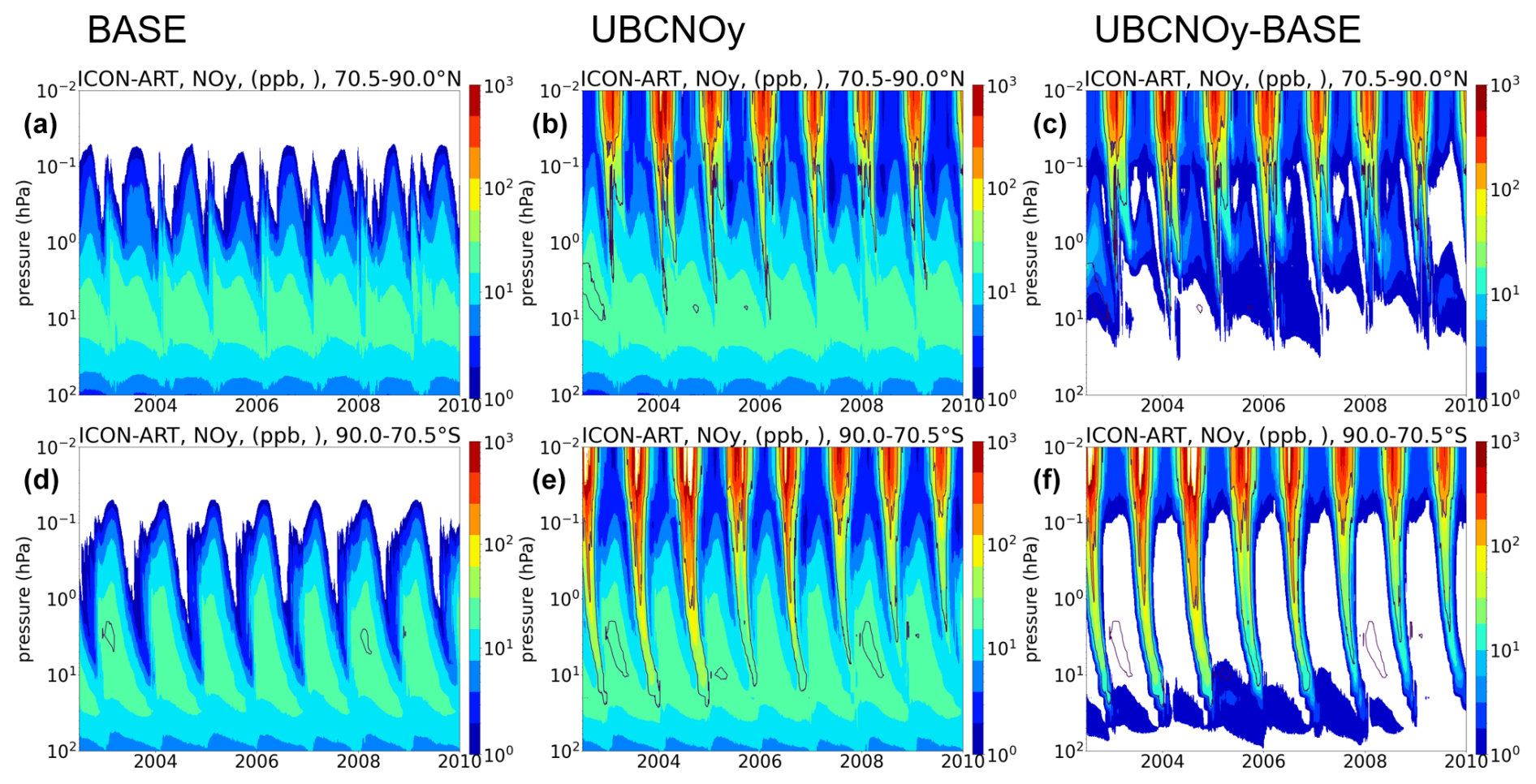
Figure 1 Daily mean, area-weighted NO_y in 70–90° N (a–c) and 70–90° S (d–f) from ICON-ART. (a, d) Experiment 1 (BASE), (b, e) experiment 2 (UBC-NO_y), and (c, f) difference (UBC-NO_y − BASE). Model runs are shown in May 2002–2010 only to allow for 2.5 years of spinup.

In Fig. 1, we show a comparison of ICON-ART without and with UBC-NO_y. The inclusion of UBC-NO_y leads to a strongly enhanced NO_y at the model top, particularly during polar winter, as well as a downward-propagating “tongue” of NO_y indicating transport from the upper mesosphere into the mid-stratosphere during every polar winter. Qualitatively, ICON-ART with UBC-NO_y well reproduces the known behavior of EPP-NO_y, with interhemispheric differences due to the differing dynamics of the high-latitude northern and southern winter middle atmosphere.

4.2 Including the NO_y-based tendency term in ICON-ART-LINOZ

In the next step of our development, we utilized LINOZ, as described in Sect. 2.3, to incorporate an NO_y-based tendency term that accounts for ozone changes in the polar stratosphere into the linearized ozone description. It is important to acknowledge that when using upper boundary NO_y values, especially within the NO_y tongue region, significant deviations from the climatological state occur. To enhance the reliability of the tendencies of ozone related to NO_y, we have re-calculated the LINOZ tables (Hsu and Prather, 2010) using a climatological NO_y with upper boundary values. It is important to note that ICON is free-running, so the specific upper boundary condition used does not correspond to the model's dynamics.

In this implementation, the J-NO photolysis rates were extended to cover the mesosphere. For this purpose, rates were derived from the EMAC model, ensuring that photochemical processes relevant above the stratosphere are appropriately represented. However, the NO_y tendencies themselves were not recalculated for different solar conditions.

4.3 Including the solar UV variation into ICON-ART-LINOZ

In addition to particle forcing, we included solar UV variability in ICON-ART to account for induced ozone changes, primarily in the tropical stratosphere. The photochemical box model calculating the LINOZ tables applies a solar spectrum provided in 77 spectral bins. In order to implement solar spectral variations, the LINOZ tables must be recalculated using solar spectra representing solar maximum and solar minimum conditions. The spectra applied are based on two spectra taken during the ATLAS missions in November 1989 (solar maximum) and 1994 (solar minimum) and prepared as described in Kunze et al. (2020) to comply with recent measurements of the solar constant. After transferring the spectra to the 77 spectral bins of the photochemical box model (Hsu and Prather, 2010; McLinden et al., 2000) (here version 8.0) we calculated two sets of tables and used them for solar maximum and solar minimum runs.

Furthermore we calculated the values for the monthly mean 10.7 cm flux under both maximum and minimum conditions (November 1989 and November 1994) and applied a linear interpolation based on the F10.7 solar activity index between these two states within the model.

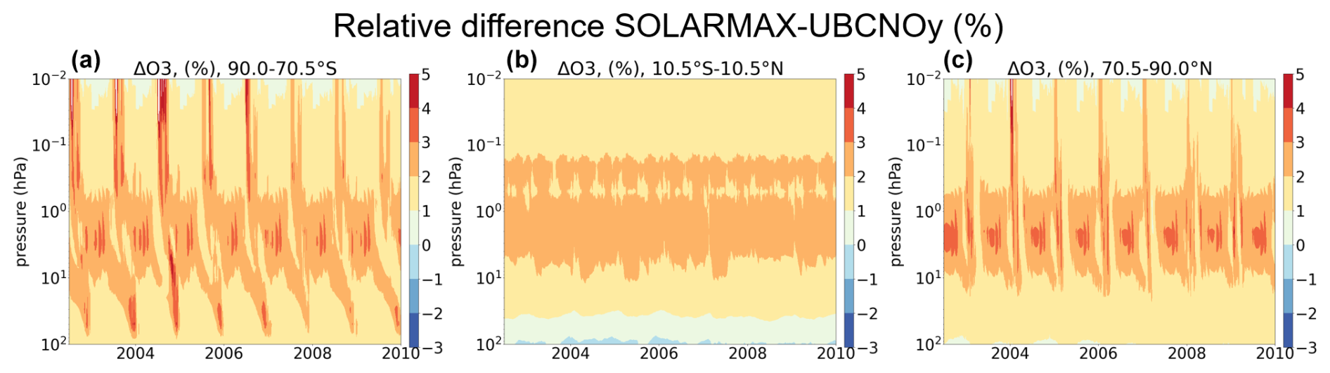
Figure 2 Impact of SSI changes on ozone in ICON-ART (Percentage difference between SOLMAX and UBC-NO_y relative to UBC-NO_y). From left to right: 70–90° S, 10° S–10° N, 70–90° N respectively.

Figure 2 shows the impact of variable SSI as the percentage difference in ozone between solar maximum (experiment SOLMAX) and solar minimum conditions (experiment UBC-NO_y), here relative to the results of the UBC-NO_y experiment. larger ozone values, in the range of a few percent, align with observed solar signals in stratospheric ozone. Higher values at high latitudes could reflect the influence of the Brewer–Dobson circulation (Brewer, 1949) and mesospheric meridional circulation, which transport ozone from the tropical stratopause source regions to the polar mesosphere in summer and to the polar lower stratosphere in all seasons. This purely chemical impact in reality could be masked by the feedback between ozone increase and changes in radiative heating, which are not considered here.

5 Evaluation of the particle and solar forcing

In the following, we will evaluate the changes made to ICON-ART. ICON-ART NO_y combining with UBC-NO_y is compared against published model results from EMAC and against MIPAS observations in Sect. 5.1, the resulting ozone fields and ozone change due to the additional NO_y and solar cycle implementation in LINOZ are discussed in Sect. 5.2.

5.1 UBC-NO_y

As shown in Fig. 3, after the implementation of the UBC-NO_y, we observe a high level of qualitative agreement at the top of the atmosphere between ICON-ART and a model simulation with the EMAC model also using the UBC-NO_y from Funke et al. (2016). The EMAC model employs MECCA stratospheric chemistry, specified dynamics relaxing towards ERA-interim reanalysis data (Dee et al., 2011), and variable geomagnetic forcing for 2000–2010 (Sinnhuber et al., 2018). Despite using the same parameterization of EPP-NO_y, some differences between ICON-ART and EMAC NO_y are apparent already at the top of the atmosphere due to differences in vertical transport and mixing.

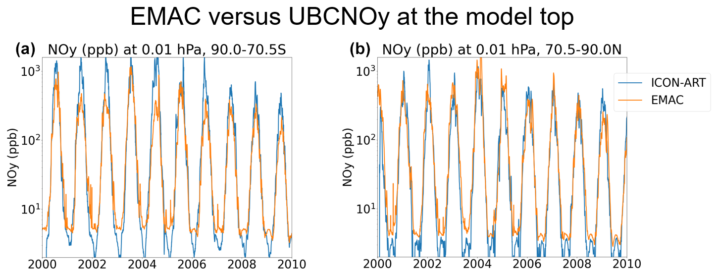
Figure 3 Daily mean, area weighted NO_y at 0.01 hPa in 70–90° S (a) and 70–90° N (b) from the chemistry-climate model ICON-ART (experiment 2, UBC-NO_y) and EMAC model results from Sinnhuber et al. (2018), also using the NO_y upper boundary condition of Funke et al. (2016).

In Fig. 4, NO_y from ICON-ART with UBC-NO_y is compared with results from the EMAC model including UBC-NO_y, and with MIPAS/ENVISAT v5 NO_y. All three data-sets reveal a significant agreement in temporal variation, vertical coverage, and interhemispheric differences particularly in the downward propagating “tongues” of NO_y during polar winters. Small differences in the year-to-year variability particularly in the Northern hemisphere are likely due to the different middle atmosphere dynamics in the free-running ICON experiments. Stratospheric NO_y is generally higher in ICON-ART than in EMAC and MIPAS. This is even true for experiment 1 (BASE), so presumably is a feature of the simplified NO_y used for the stratospheric background. During the Northern Hemisphere winter of 2003/2004, NO_y penetrated deeply into the stratosphere, with values of 100 ppb around 48 km per 1 hPa in ICON-ART, in good agreement with EMAC and MIPAS. Due to the stronger stratospheric polar vortex in the Southern hemisphere winter, NO_y is transported further down into the stratosphere there, again in good agreement between ICON-ART with UBC-NO_y, EMAC, and MIPAS.

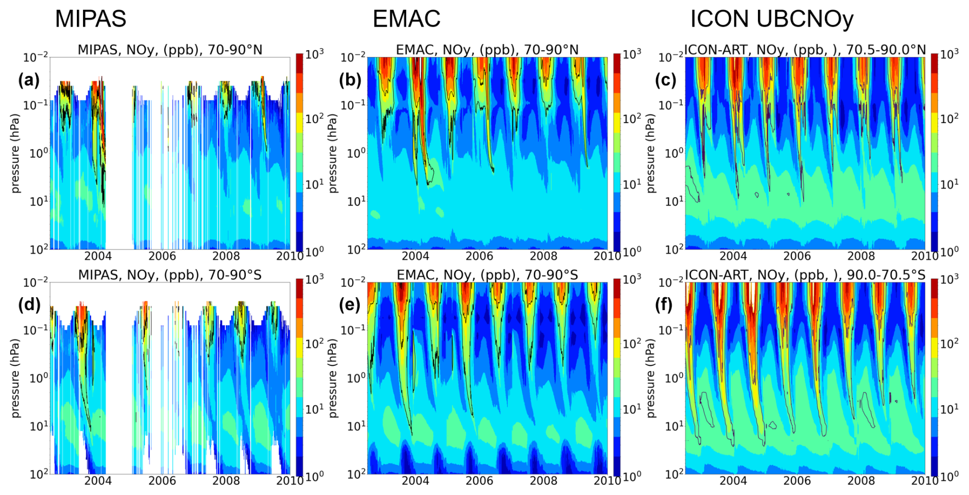
Figure 4 Daily mean, area-weighted NO_y in 70–90° N (a–c) and 70–90° S (d–f) from (a, d) MIPAS/ENVISAT v5, (b, e) EMAC, and (c, f) ICON-ART (UBC-NO_y). EMAC and MIPAS data are from Sinnhuber et al. (2018).

In Fig. 5, EPP-NO_y in ICON-ART, shown as the differences between the UBC-NO_y and BASE simulations, is compared to EMAC and MIPAS/ENVISAT v5. The result indicates that both models demonstrate a high degree of qualitative consistency with observations during winter. The EMAC model shows better agreement due to its specified dynamic mode. In both models, EPP-NO_y persists into summers in a very consistent way. This is not evident in the observations and could be attributed to the sensitivity cutoff related to the NO_y/CO correlation used to derive EPP-NO_y from MIPAS/ENVISAT data.

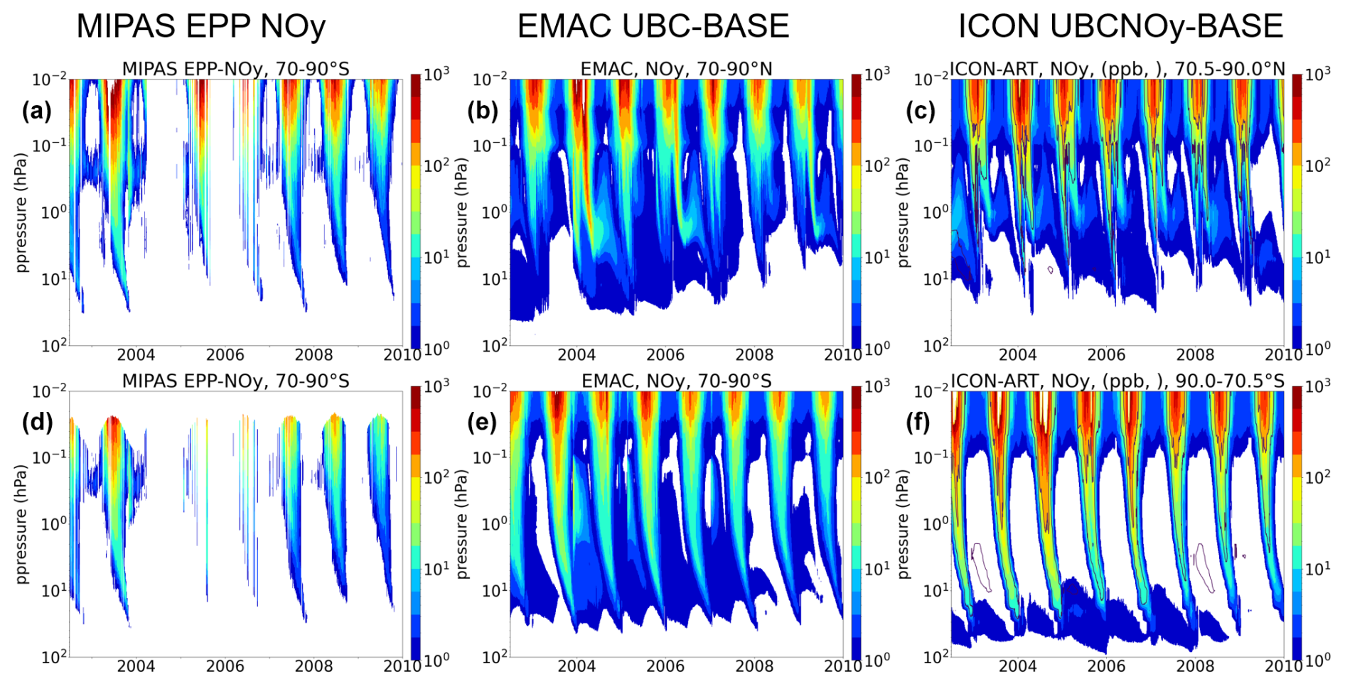
Figure 5 Daily mean area-weighted EPP-NO_y. (a, d) MIPAS/ENVISAT v5 adapted from Sinnhuber et al. (2018); (b, e) EMAC, difference from model run with UBC-NO_y to base run without UBC-NO_y but identical in every other respect (Sinnhuber et al., 2018); (c, f) ICON UBC-NO_y-BASE.

The addition of the particle forcing due to the indirect effect of EPP to the linearized ozone chemistry leads to a substantial decrease in ozone in the polar upper and mid-stratosphere in both hemispheres because of catalytic cycles that involve NO_x.

Figure 6 indicates the mixing ratio of the ozone fields after inclusion of the NO_y-based tendency in ICON-ART-LINOZ version 3 in both the Northern and Southern high latitudes compared to EMAC and MIPAS/ENVISAT v5. Comparison against the EMAC model and MIPAS/ENVISAT v5 observation shows a good agreement in the absolute values, temporal coverage of ozone change, vertical coverage and variability, as well as interhemispheric differences (Sinnhuber et al., 2018).

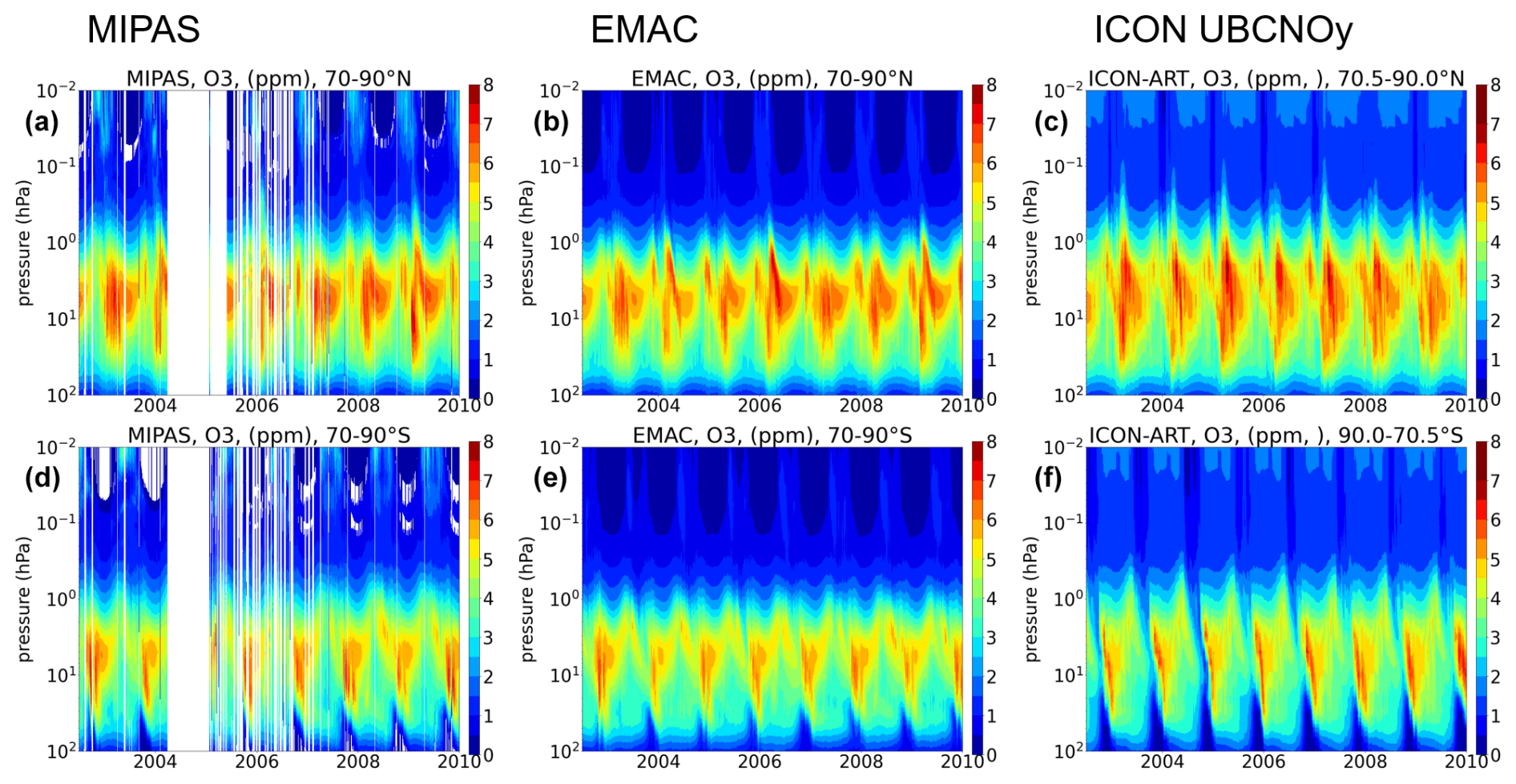
Figure 6 Daily mean, area weighted ozone after inclusion of the NO_y-based tendency in 70–90° N (a–c) and 70–90° S (d–f) from (a, d) MIPAS/ENVISAT v5, (b, e) EMAC, and (c, f) ICON UBC-NO_y. The EMAC and MIPAS data are from Sinnhuber et al. (2018).

The pronounced simulated low ozone values in the Southern hemisphere lower stratosphere during polar winter and spring are consistent with the Antarctic ozone hole.

Figure 7 shows the ozone change due to EPP-NO_y for high Northern latitudes (70 to 90° N) and high Southern latitudes (70 to 90° S), for ICON-ART and EMAC. The range of values, morphology, and interhemispheric differences between the two models are consistent. The slightly larger decreases in the Southern hemisphere observed in ICON may indicate stronger downwelling and a more persistent vortex, aligning with the slightly higher EPP-NO_y levels. This phenomenon is less evident in the Northern hemisphere, which could be due to differences in the model dynamics.

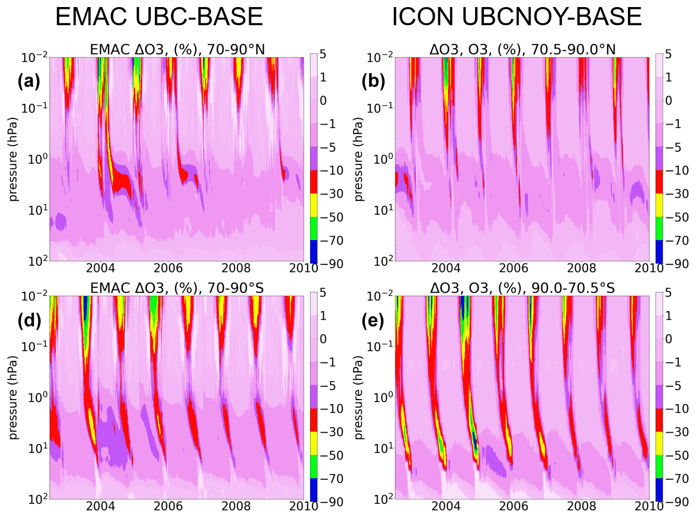
Figure 7 Daily mean area-weighted ozone change due to EPP-NO_y in percentage in 70–90° N (a, b) and 70–90° S (c, d) from (a, c) EMAC (Sinnhuber et al., 2018), and (b, d) ICON-ART. The contour intervalls are the same as in Sinnhuber et al. (2018) (Figs. 12 and 13).

Areas of low ozone develop in the mesosphere during the early winter months and descend to the mid-stratosphere by late winter/early spring in the Northern hemisphere. In the Southern hemisphere, they develop in the mesosphere during late winter/early spring and decline to the mid-stratosphere by early summer. This negative ozone response persists into the subsequent winter of 2004 around 1–10 hPa of the Northern hemisphere in both models (see Fig. 7). The persistent early summer ozone depletion observed in the ICON model during 2003 may be linked to an Elevated Stratospheric (ES) event (Manney et al., 2008) that occurred early in that year. EMAC does not show a similar ES event for 2003, while the 2006 ES event present in EMAC is not captured by ICON. These discrepancies highlight the variability in how the two models represent such events.

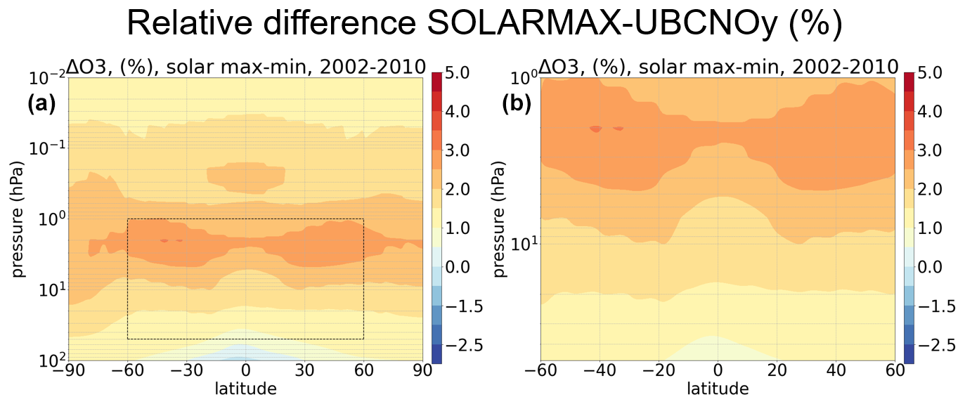
Figure 8 Impact of solar spectral irradiance (SSI) on ozone in ICON-ART: Percentage difference between SOLMAX and UBC-NO_y relative to UBC-NO_y (a). Same, but with pressure and latitude range adapted to ozone solar signal figures (two different datasets – SAGEII/SBUV) in Maycock et al. (2016) (b).

5.2 Solar UV variation

The impact of SSI on ozone in ICON-ART (solar maximum minus solar minimum) is shown in Fig. 8. Differences of up to 4 % in the mid- and low-latitude stratosphere are observed in ICON-ART and are in good agreement with, and within, the large spread of observations (compared, e.g., to Maycock et al., 2016, their Figs. 4 and 12). Differences in structure could be attributed to missing radiative and dynamical feedback. At high latitudes, higher values of more than 3 % are shown. However, these cannot be compared directly against observations, as at high latitudes, the much larger changes due to particle precipitation mask the smaller changes caused by UV variability.

6 Conclusion

We have presented a new method of incorporating a top-down solar forcing into the stratospheric ozone, triggered by the EPP indirect effect, by utilizing a semi-empirical model for NO_y based on the geomagnetic A_p index (Funke et al., 2016). This provides a more realistic representation of the stratospheric NO_y densities and its wintertime downward transport. This new implementation of the nitrogen chemistry in ICON-ART will help improve the prediction of the ozone field in the model as a direct response to NO_y.

The addition of geomagnetic forcing led to significant ozone losses in the polar upper stratosphere of both hemispheres due to the catalytic cycles involving NO_y. Comparing to EMAC (Sinnhuber et al., 2018) and MIPAS (Funke et al., 2014a) ICON-ART agrees well in the upper stratosphere (1 hPa), but it overestimates the transport into the stratosphere, leading to an overestimation of NO_y in the mid-stratosphere (at and below 10 hPa) in many (but not all) winters. The maximum ozone loss in the mid to upper stratosphere due to the indirect effect of EPP occurs in late winter to spring.

Considering the solar UV variability in the ICON-ART model leads to the changes in ozone in the tropical stratosphere, which is in agreement with observations (Maycock et al., 2016).

In conclusion, our study demonstrates that the inclusion of solar forcing, specifically particle precipitation and solar UV radiation, in the ICON-ART model relying on linearized ozone scheme provides realistic ozone fields.