Soil parameterization in land surface models drives large discrepancies in soil moisture predictions across hydrologically complex regions of the contiguous United States

Land surface models (LSMs) are critical components of Earth system models (ESMs), enabling the simulation of energy and water fluxes that are essential for understanding climate systems. Soil hydraulic parameters, derived using pedotransfer functions (PTFs), are crucial for modeling soil–plant–water interactions; they introduce uncertainties in soil moisture simulations. However, a key knowledge gap exists in understanding how specific soil hydraulic properties contribute to these uncertainties and in identifying the regions most affected by them. This study conducts an intra-model sensitivity analysis within the Community Land Model version 5 (CLM5), examining how alternative soil parameter settings influence soil moisture variability across the contiguous United States (CONUS) using empirical orthogonal function (EOF) analysis. The EOF analysis revealed dominant spatial and temporal patterns of soil moisture across multiple experimental configurations, highlighting the impact of soil parameter variability on hydrological processes. The results showed significant discrepancies in soil moisture simulations, particularly in the central Great Plains, which may be attributed to the combination of arid climatic conditions and limitations in modeling saturated hydraulic conductivity and soil water retention curves. Seasonal soil moisture dynamics showed broad similarity to ERA5-Land patterns, with differences in magnitude and phase, indicating the importance of refined parameterization, particularly in the representation of infiltration and drainage processes. Comparisons with ERA5-Land, used here solely as a model-based reference for pattern consistency, revealed stronger similarity in regions with consistent climatic gradients but persistent differences in hydrologically complex areas, particularly in areas with arid climates, such as the Great Plains, where hydrological processes remain difficult to represent. Because CLM5 is forced by GSWP3, whereas ERA5-Land is an offline HTESSEL replay forced by ERA5, differences reflect both forcing and structural contrasts in addition to parameter effects. This research demonstrates the necessity to refine soil parameter representations, utilize high-resolution datasets, and consider climatic variability to inform the model development of LSMs. Importantly, these findings also pave the way for future efforts that incorporate dynamic soil properties into LSMs. This work illustrates the influence of soil properties on simulated variability. While the analysis documents their importance, a future direction will be to develop approaches that allow these properties to vary dynamically within LSMs. This study contributes to ongoing efforts toward more integrated modeling frameworks that capture soil–hydrology–climate interactions.

1 Introduction

Land surface models (LSMs) are essential components of Earth system models (ESMs), offering critical insights into the movement and partitioning of energy and water across the Earth's surface, which are fundamental processes in understanding and simulating climate systems accurately (Kang and Hong, 2008; Zhao et al., 2017; Guimberteau et al., 2017; Hagemann et al., 2013; Dagon et al., 2020). Designed to operate on large spatial scales, LSMs rely on parameterizations of land processes, including the use of pedotransfer functions (PTFs) to parameterize soil hydraulic properties. PTFs, as described by Van Looy et al. (2017) and De Lannoy et al. (2014), are mathematical formulations that use extensive soil hydraulic databases to establish empirical relationships between soil particle and soil hydraulic parameters, such as field capacity, permanent wilting point, saturated hydraulic conductivity, pore-size distribution, and soil water retention curves (McNeill et al., 2018; Vereecken et al., 2010; Weber et al., 2020). These PTFs range in complexity from basic linear models to advanced machine learning algorithms such as artificial neural networks (da Silva et al., 2023; Schaap et al., 1998). These soil hydraulic parameters are fundamental to the quantification of soil moisture and water flow, as well as soil–plant–water interactions and their effects on climate, agriculture, hydrology, and environmental engineering.

PTFs play a crucial role in converting readily available soil texture data into soil hydraulic parameters, addressing the difficulties of acquiring accurate soil moisture data at larger scales (Fu et al., 2023). However, many soil hydraulic parameters are derived from laboratory or small-scale field studies, which often fail to capture the full heterogeneity of larger areas, limiting their representativeness (Lai and Ren, 2016; Godoy et al., 2018). To overcome this limitation, global soil texture maps enhance PTFs' predictive capabilities, enabling their application in regions where field measurements are unavailable and making them indispensable for land modeling (Tafasca et al., 2020; Dai et al., 2019). Soil moisture, a key output of these models, is a vital variable governing the exchange of water and energy between the land and atmosphere. It has profound impacts on climate systems, vegetation dynamics, and extreme events, including droughts and floods (Zhang et al., 2021).

The influence of soil hydraulic properties on soil moisture simulations is well documented. For example, Fu et al. (2023) demonstrated that these properties significantly affect soil moisture simulations at the ELBARA field site in the northeast of the Tibetan Plateau, using the one-dimensional (1D) Richards equation. Similarly, Fu et al. (2022) noted that the numerical solution approach of the Community Land Model (Lawrence et al., 2019) produces a narrow range of soil hydraulic property values, which suggests a relatively weak influence on soil moisture simulations within this range. However, when optimized hydraulic properties are used, potentially derived to capture site-specific variability or improve model similarity beyond this narrow range, they can exert a more substantial influence on soil moisture dynamics. Furthermore, Feki et al. (2018) showed that saturated hydraulic conductivity exhibits the highest sensitivity to temporal changes in environmental factors, such as precipitation or temperature variability, significantly affecting soil moisture variability, as shown in the FEST-WB model simulation of a maize field in the Secugnago region. These findings underline the importance of accurately representing soil hydraulic properties, which directly influence the partitioning of water into runoff, infiltration, and evapotranspiration (Ye et al., 2023), as well as the temporal and spatial variability in soil moisture. However, uncertainties in parameterizations, such as the soil water retention curve that links water potential to volumetric soil moisture, continue to challenge the predictive capacity of LSMs, especially under extreme climatic conditions (Koster et al., 2004; De Lannoy et al., 2014). Improving the representation of soil moisture and its underlying hydraulic properties is critical, as it affects global hydrological cycles, vegetation health, and energy flows, all of which are essential for understanding and mitigating the impacts of climate events (Oleson et al., 2010).

In addition to these complexities, scaling point-scale or regional observations of soil moisture to the coarser resolutions of LSM outputs presents a persistent challenge. While observational networks and remote-sensing missions have expanded the availability of soil moisture data, the heterogeneous nature of soil properties combined with varying retrieval algorithms and coverage gaps can introduce significant uncertainties, both in terms of the accuracy of satellite products and their limitations for validating LSM outputs (Famiglietti, 2014; Brocca et al., 2017). Moreover, uncertainties in parameterization make it challenging to accurately simulate soil moisture dynamics, as noted by Reichle et al. (2004) and Kato et al. (2007), limiting the ability of LSMs to replicate observed soil moisture datasets. This discrepancy in spatial resolution and data precision can make model calibration more challenging, increase uncertainties in estimating parameters, and (as a result) weaken confidence in simulation outputs. Emerging evidence further complicates this issue by highlighting that soil properties can change over relatively short timescales due to shifts in climate and land cover. The dynamic nature of soil properties introduces additional pressure to understand soil–hydraulic relationships better and integrate these temporal dynamics into LSMs, as demonstrated by studies indicating how climate and land cover changes influence soil processes (Hirmas et al., 2018; Koop et al., 2023; Caplan et al., 2019; Sullivan et al., 2022; Hauser et al., 2022). Addressing these complexities requires robust, data-driven approaches and dimensionality reduction techniques to disentangle the effects of parameterization on soil moisture patterns across various ecosystems and climatic conditions.

A major challenge to addressing these uncertainties is the high dimensionality of LSM simulations when applied to continental or global scales, making it difficult to isolate the effects of specific parameters on soil moisture from other factors such as meteorological forcings and modes of climate variability (Ji et al., 2023; Li et al., 2013; Zeng et al., 2021). Therefore, we present an intra-model sensitivity analysis within CLM5, focusing on how alternative soil hydraulic parameter datasets propagate into regional soil moisture patterns and variability, without treating any external product as the ground truth. Specifically, we ask the following questions:

1. How do soil hydraulic parameters influence large-scale spatial patterns in soil moisture associated with well-characterized climate variability modes?

2. How do these parameters shape the temporal dynamics of soil moisture during climate extremes, such as droughts and floods?

Using empirical orthogonal function (EOF) analysis, we systematically evaluate the impact of soil hydraulic parameterizations in CLM5 simulations over the contiguous United States (CONUS). We compare the spatial and temporal patterns of CLM5 with those in ERA5-Land using pattern-similarity metrics (e.g., correlation, Taylor diagrams, and Euclidean distance). ERA5-Land is used solely as a model-based reference for patterns; it does not assimilate soil moisture observations and is not treated as the ground truth. We note an upfront forcing and structural mismatch: our CLM5 experiments are driven by GSWP3, whereas ERA5-Land is an offline HTESSEL replay forced by ERA5; therefore, the differences reflect both forcing and structural contrasts, as well as parameter effects. (Neither product includes irrigation, so agricultural hotspots should not be overinterpreted.) We aim to transparently document where parameter uncertainty most affects simulated soil moisture patterns and variability across CONUS and to provide disciplined evidence to inform model use and development. We next outline the data sources, EOF methods, and computational steps; present principal findings on soil moisture variability and parameter sensitivity; and detail the broader implications for land surface modeling and climate dynamics.

2 Data and methods

2.1 Study region

The study region for this analysis encompasses the CONUS, spanning from the Atlantic Ocean to the Pacific Ocean and bounded by Canada to the north and Mexico to the south (Fig. 1). This domain encompasses a wide range of latitudes, elevations, and climatic regimes, providing an ideal natural laboratory for assessing spatial variability in land surface processes. The CONUS encompasses major climate zones, including humid continental, Mediterranean, subtropical, arid, and alpine, all of which are influenced by differences in latitude, topographic relief, and proximity to moisture sources such as the Gulf of Mexico and the Pacific Ocean. These climatic gradients play a critical role in controlling soil moisture dynamics by modulating processes such as infiltration, evaporation, and water retention. Topographic features, including the Rocky Mountains, Sierra Nevada, Cascade Range, and Appalachian Mountains, have a significant influence on precipitation regimes and surface hydrology. These orographic barriers modify storm tracks and induce spatial variability in rainfall and snowpack accumulation, ultimately affecting soil water availability. The land cover across the CONUS is equally heterogeneous, ranging from forested regions in the Northeastern United States and Pacific Northwest to urbanized corridors and sparsely vegetated deserts in the Southwestern United States. This heterogeneity in land cover introduces additional complexity into soil moisture behavior, as vegetation, impervious surfaces, and soil types interact to determine local infiltration and storage dynamics.

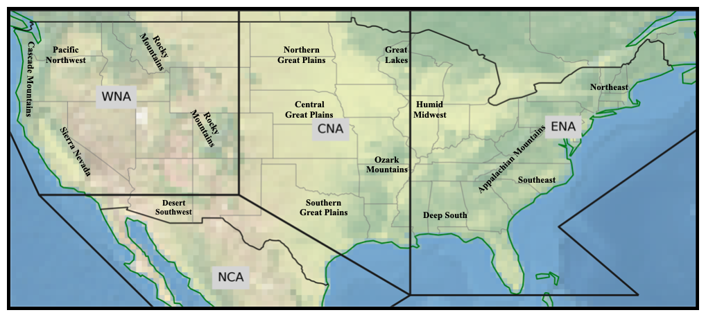
Figure 1 Regional divisions of the CONUS area into four major zones: western North America (WNA), central North America (CNA), eastern North America (ENA), and northern Central America (NCA), as defined by Giorgi and Francisco (2000), based on climate variability and geographical features. Prominent subregions and geographical landmarks, such as mountain ranges and plains, are also depicted.

To support spatially disaggregated analysis of soil moisture variability and its driving mechanisms, we adopt the regional classification scheme proposed by Giorgi and Francisco (2000), which partitions CONUS into four climatically and geographically coherent macro-regions: western North America (WNA), central North America (CNA), eastern North America (ENA), and northern Central America (NCA). This classification provides a physically grounded framework for evaluating the sensitivity of modeled soil moisture to soil hydraulic parameterizations across distinct hydroclimatic zones. As shown in Fig. 1, each region captures distinct physiographic and climatic attributes, including the arid basins and mountain ranges of WNA, the agricultural plains and grasslands of CNA, the humid subtropical and deciduous forest zones of ENA, and the transitional climatic conditions present in NCA. The utility of this framework is twofold: first, it facilitates regional intercomparison of soil moisture patterns and their controls, enabling consistent evaluation across diverse landscapes; second, it improves the interpretability of EOF modes by linking observed spatial variability to regional climatic drivers, soil texture distributions, and vegetation structure. This regionalized approach is particularly valuable given the goal of disentangling parameter-driven soil moisture responses from broader meteorological forcings. By leveraging the CONUS domain and its subdivisions, the study advances understanding of how soil hydraulic parameter uncertainty manifests across large-scale gradients and informs the development of improved land surface model parameterizations.

2.2 Data description

The Soil Parameter Intercomparison Project (SP-MIP), initiated at the GEWEX-SoilWat workshop in Leipzig (2016), aims to quantify the variability in land surface model (LSM) output caused by differences in soil parameters and structures. Following the Land Surface, Snow, and Soil Moisture Model Intercomparison Project (LS3MIP) protocol (van den Hurk et al., 2016), SP-MIP brought together eight leading LSMs – CLM5, ISBA, JSBACH, JULES, MATSIRO, MATSIRO-GW, NOAH-MP, and ORCHIDEE – for a series of global simulation experiments (Gundmundsson and Cuntz, 2017). These models were run on a 0.5° grid and forced with Global Soil Wetness Project Phase 3 (GSWP3) meteorological data for 1980 to 2010. We use CLM5 output produced by the National Science Foundation (NSF) National Center for Atmospheric Research (NCAR) for SP-MIP (Thornton, 2010; Lawrence et al., 2019). The dataset covers global landmasses at 0.5° resolution (25 920 grid cells, excluding waterbodies and permanent snow/ice) and includes 41 land surface variables such as evapotranspiration, soil temperature, and runoff, spanning 30 years (1980 to 2010). The global soil profile reaches a depth of 41.998 m with 25 layers; however, for this study, soil moisture was extracted from depths (0–1.0 m) containing the most roots (root zone) of the CONUS region, covering 6413 grid cells. The focus is on the variable water content of soil layers (mrsol) to explore soil moisture variability and distribution. Importantly, irrigation is not represented; all simulations are under rainfed (naturalized) conditions to isolate the influence of soil hydraulic parameterizations without additional anthropogenic water inputs. ERA5-Land (ECMWF) is also used as a model-based pattern reference (not the ground truth). It is an offline land surface replay forced by ERA5 and does not assimilate soil moisture observations. For consistency, ERA5-Land fields were regridded to 0.5° to match CLM5. Note the forcing mismatch (CLM5: GSWP3; ERA5-Land: ERA5), so differences reflect both forcing and structural contrasts as well as parameter effects.

2.2.1 Experimental designs

Four experimental designs were implemented to isolate the effects of soil properties on hydrological and energy balance variables. Soil parameters for Experiment 1 (EXP1) and soil textures for Experiment 2 (EXP2) were derived at a 0.5° resolution, based on dominant soil classifications within the 0–5 cm layer of SoilGrids data (Hengl et al., 2014) at a 5 km resolution. The Brooks–Corey parameters are derived from Table 2 of Clapp and Hornberger (1978), while the Mualem–van Genuchten parameters represent ROSETTA class average hydraulic values as cited by Schaap et al. (2001), with soil textures taken from Table 1 of Cosby et al. (1984). For experiments 4a–d (EXP4a–EXP4d), the USDA soil categories used are loamy sand, loam, silt, and clay, as defined by Montzka et al. (2011). These experiments employ identical transfer functions for the Brooks–Corey and the Mualem–van Genuchten parameters, as applied in Experiment 1 (EXP1). CLM5 solves the Richards equation for the movement of soil water. The provided soil parameters and textures are uniform throughout the entire soil column. For a detailed description of the SP-MIP dataset, please refer to Gundmundsson and Cuntz (2017). The schematic (Fig. 2) summarizes the CLM5 workflow and experimental grouping, which consists of four designs yielding seven runs (EXP1, EXP2, EXP3, and EXP4a–EXP4d), used to assess how soil hydraulic parameterizations influence soil moisture variability.

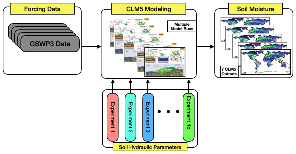
Figure 2 Experimental setup for evaluating soil moisture variability in CLM5. The model utilizes GSWP3 forcing data and conducts multiple experiments with varying soil hydraulic parameterizations. EXP1 applies standardized parameters, EXP2 derives parameters from soil texture, EXP3 uses default CLM5 settings, and EXP4a–EXP4d assign uniform parameters for different soil types.

Table 1 Soil parameters for the three selected water retention curves were supplied by SP-MIP as input for experiments 1 and 4a–d.

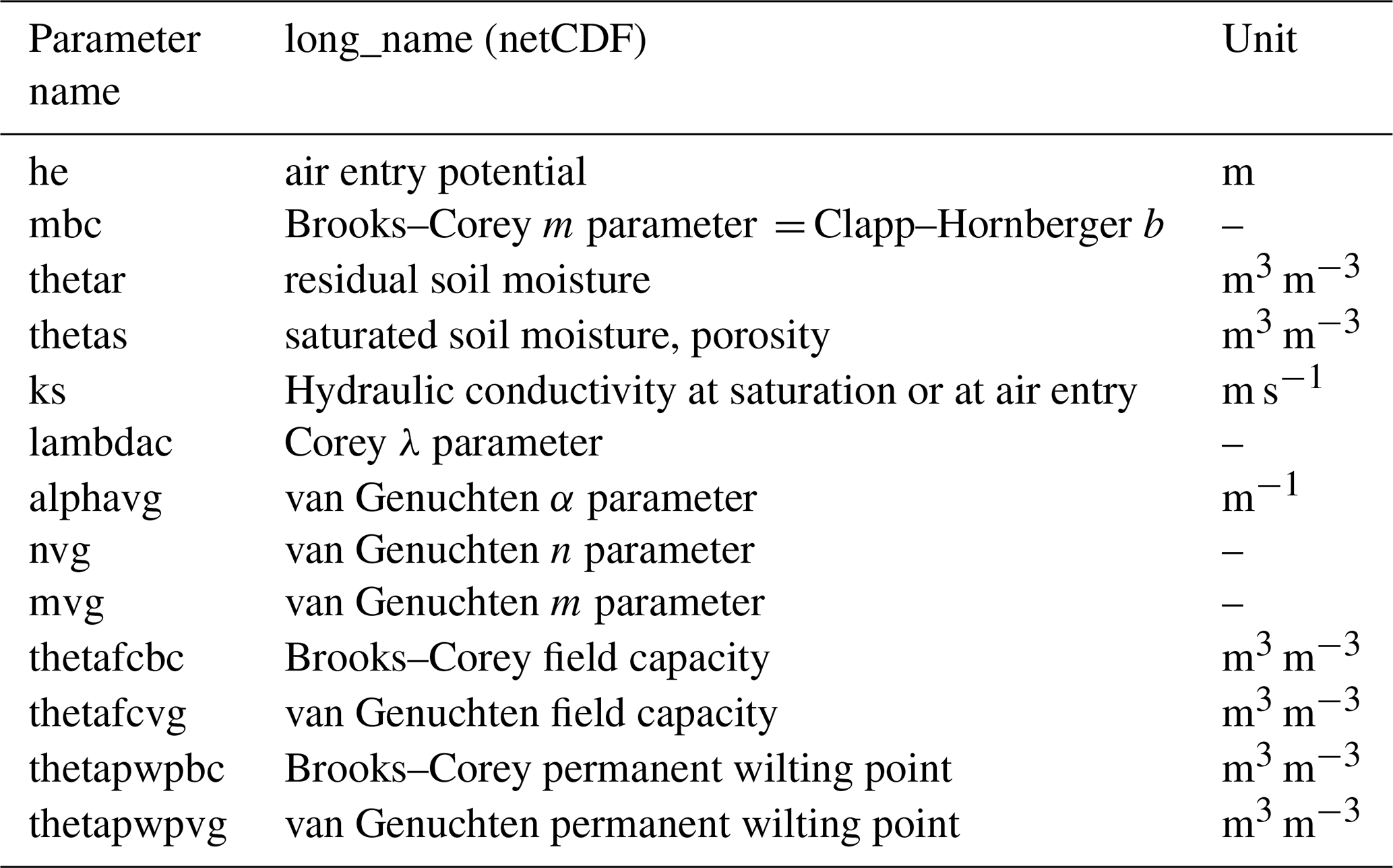
Table 2 Soil textural characteristics supplied by SP-MIP for experiment 2.

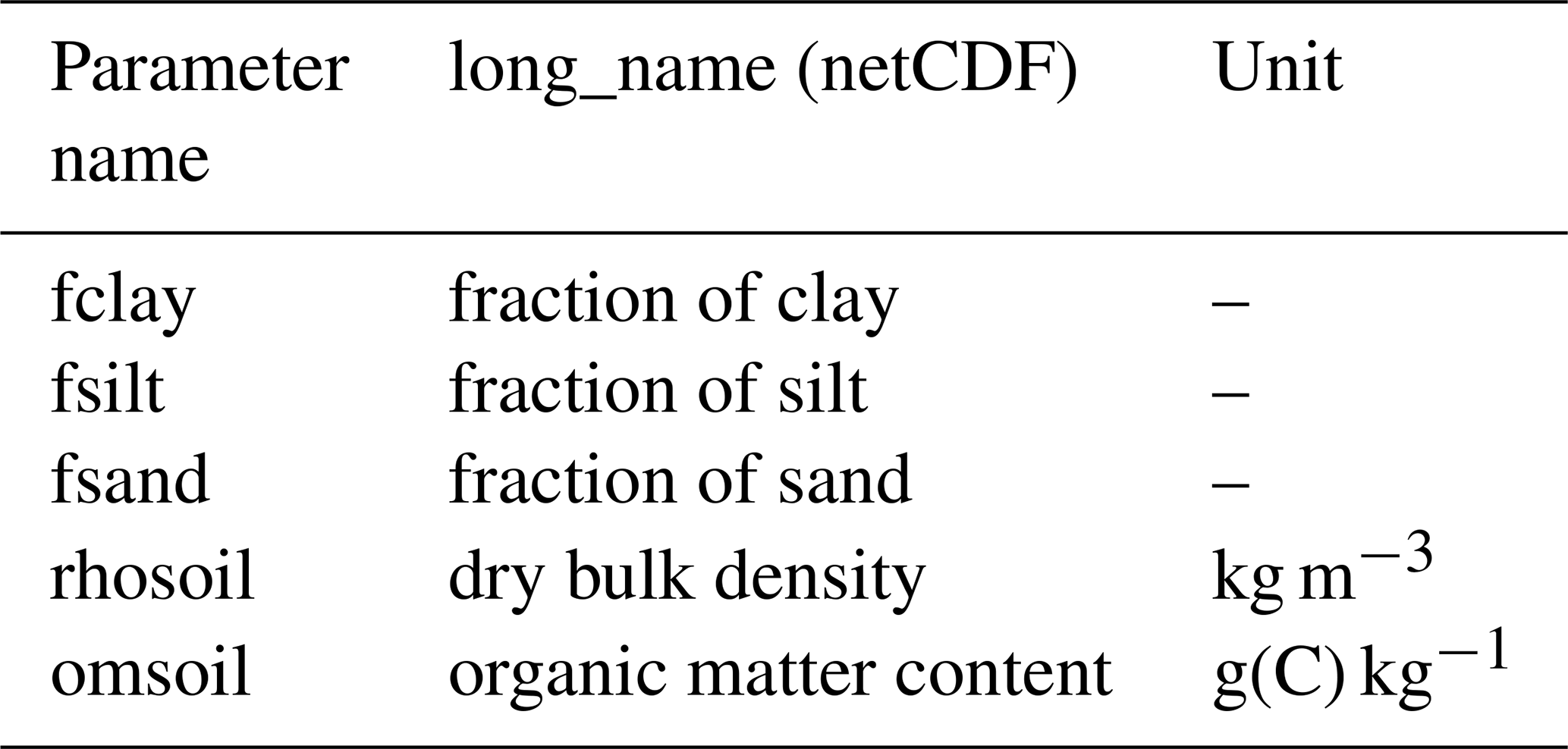
Table 3 Summary of the SP-MIP experimental configurations analyzed in this study. EXP1–EXP2 use prescribed SP-MIP inputs at 0.5°; EXP3 uses CLM5 defaults; EXP4a–EXP4d are globally uniform design soils. Analyses use root-zone soil moisture extracted from each experiment from 1980 to 2010.

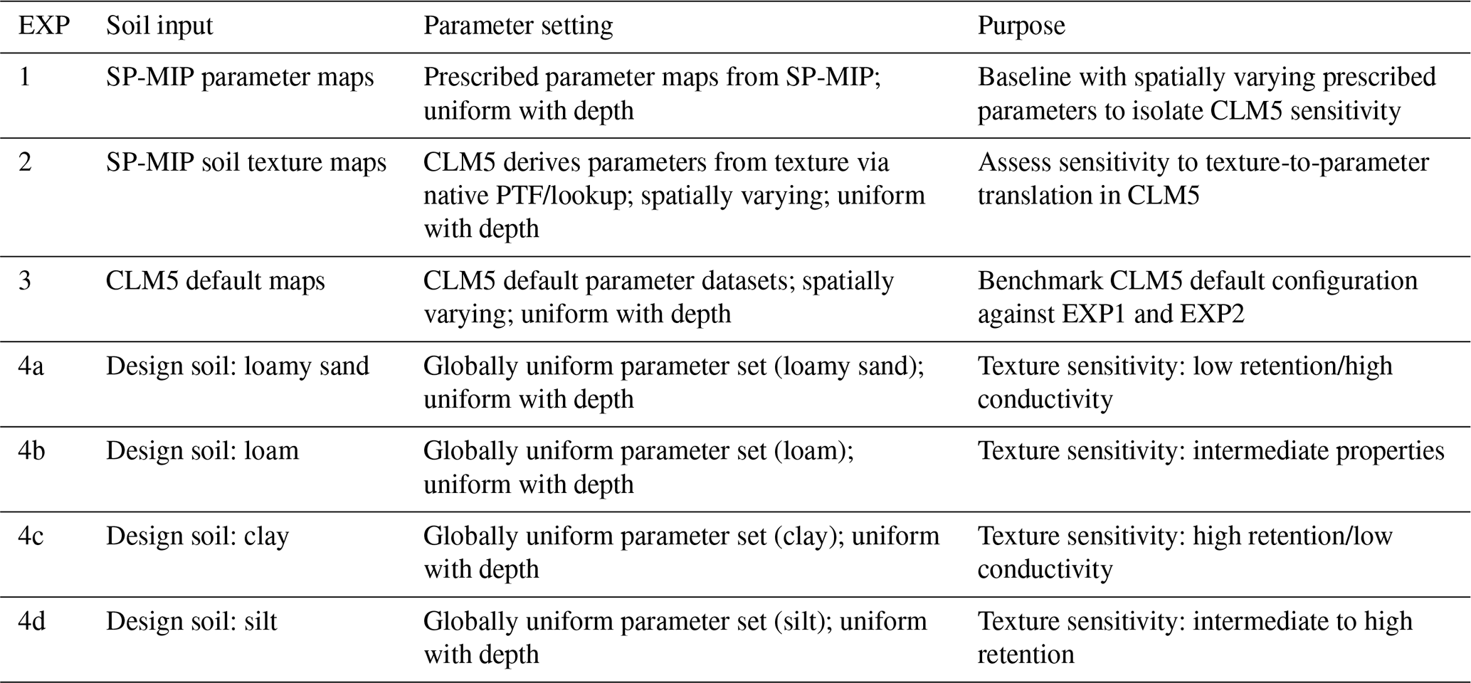
To assess the influence of soil hydraulic parameterizations on soil moisture variability within the CLM5, a series of simulations were conducted following the SP-MIP framework (Gundmundsson and Cuntz, 2017). Although SP-MIP was designed for multi-model comparisons, we adapted it to evaluate intra-model variability within CLM5 by varying soil hydraulic parameter sets. All simulations used consistent meteorological forcing (GSWP3), spatial resolution (0.5°), and spanned 1980 to 2010, with a standardized spin-up routine to ensure reliable initial conditions. Below, we describe the four experimental setups, their objectives, configurations, hypotheses, and expected outcomes, focusing on how parameters are applied within CLM5. Each experiment followed the standard CLM5 spin-up procedure to ensure that carbon, water, and energy state variables reached quasi-equilibrium prior to the simulation period, thereby minimizing the influence of initial conditions on soil moisture dynamics (Lawrence et al., 2019). Spin-up followed SP-MIP protocol guidelines to ensure equilibrium prior to the 1980 to 2010 simulation period (Gundmundsson and Cuntz, 2017). For clarity, Table 3 summarizes the soil inputs, parameter settings, and purposes of EXP1–EXP4a–EXP4d (root-zone soil moisture, 1980 to 2010). The specific experiments used are as follows:

1. EXP1 – soil hydraulic parameters provided by SP-MIP. This experiment serves as a baseline simulation, applying soil hydraulic parameters provided by SP-MIP (Table 1). These parameters, derived from PTFs such as Brooks–Corey (Clapp and Hornberger, 1978) and Mualem–van Genuchten (Schaap et al., 2001), are applied uniformly across all grid cells in the CONUS at a 0.5° resolution using GSWP3 meteorological forcing data (1980 to 2010). The objective is to establish an internal reference for soil moisture simulations by eliminating spatial variability in soil properties, allowing the isolation of CLM5's response to a consistent soil parameter set. The hypothesis is that SP-MIP soil hydraulic parameters will produce uniform soil moisture patterns, serving as a control to quantify the effects of parameter variations in other experiments. The expected outcome is a consistent baseline for intra-model comparisons, highlighting CLM5's sensitivity to parameter changes rather than inter-model differences.

2. EXP2 – texture-derived soil hydraulic parameters. In this experiment, CLM5 uses SP-MIP-provided soil texture inputs (Table 2), such as fractions of clay, silt, sand, dry bulk density, and organic matter content, to derive soil hydraulic parameters internally via its native PTFs and lookup tables. These parameters vary spatially across the CONUS domain based on textural classes. The objective is to assess how CLM5's standard approach to translating soil texture into hydraulic properties influences soil moisture outputs. The hypothesis is that spatial variability in texture-derived parameters will introduce heterogeneity in soil moisture patterns, reflecting the default parameterization practices of CLM5. The expected outcome is a simulation that mirrors operational CLM5 runs, allowing for comparison with EXP1 to assess the impact of texture-to-parameter translation on hydrological variability.

3. EXP3 – CLM5 default configuration. This experiment employs CLM5's default soil hydraulic parameters, as defined by its operational input datasets, applied to all soil layers across CONUS. Unlike EXP1's standardized parameters or EXP2's texture-derived parameters, EXP3 reflects CLM5's inherent configuration without external constraints. The objective is to evaluate the model's intrinsic variability due to its standard soil parameter settings, providing a benchmark for CLM5's default behavior. The hypothesis is that CLM5's default parameters, which vary spatially based on its native soil maps, will produce distinct soil moisture patterns compared to the controlled setups in EXP1 and EXP2. The expected outcome is a simulation that highlights the influence of CLM5's built-in assumptions on soil moisture, allowing quantification of parameter-driven variability within a single model.

4. EXP4a–EXP4d – uniform soil texture simulations. These four experiments (EXP4a: loamy sand; EXP4b: loam; EXP4c: clay; and EXP4d: silt) each involve a separate CLM5 simulation with uniform soil hydraulic parameters from SP-MIP (Table 1) applied across the entire CONUS domain. The parameters, derived from PTFs for each USDA soil class (Montzka et al., 2011), are spatially constant within each experiment but differ across the four runs based on soil type. The objective is to test CLM5's sensitivity to distinct soil textures and their associated hydraulic properties, such as porosity, saturated hydraulic conductivity, and water retention curves, and to evaluate their impact on hydrological (e.g., soil moisture) and energy balance (e.g., evapotranspiration) outputs. The hypothesis is that each soil type will produce unique soil moisture patterns, reflecting texture-dependent hydrological behavior. The expected outcome is a set of simulations that isolate the effects of soil texture on CLM5's outputs, providing insights into parameter-driven variability across diverse soil types.

2.2.2 Model-based reference for pattern comparison: ERA5-Land

ERA5-Land, produced by the European Centre for Medium-Range Weather Forecasts (ECMWF), is used here as a spatially complete, model-based reference for pattern comparison; it is not treated as a ground truth or a validation dataset. Note the forcing and structural contrasts: our CLM5 experiments are forced by GSWP3, whereas ERA5-Land is an offline HTESSEL replay forced by ERA5; therefore, differences reflect both forcing and model structure, not parameter effects alone. ERA5-Land does not assimilate soil moisture observations; it is an offline land surface replay forced by ERA5 atmospheric reanalysis fields (Muñoz-Sabater et al., 2021). Thus, land surface states are governed by HTESSEL physics and driven by ERA5 meteorology. Although ERA5-Land involves no land data assimilation, it is often used as a spatially consistent model product for pattern comparison due to its global coverage and frequent updates. However, studies have identified certain discrepancies, such as a wet bias in its soil moisture measurements relative to ground-based and Soil Moisture Active Passive (SMAP) satellite data, particularly in heavily vegetated and humid areas (Lal et al., 2022). Additionally, neither our CLM5 configuration nor ERA5-Land includes irrigation, which can significantly affect soil moisture in intensively cultivated regions. As documented in previous studies, the absence of irrigation in the HTESSEL land surface model used by ERA5-Land has been linked to the underestimation of soil moisture in irrigated areas and is a known limitation when interpreting results over agricultural landscapes (Wipfler et al., 2011; Lavers et al., 2022; Tang and McColl, 2023). These characteristics and known biases underline the need for careful interpretation when using ERA5-Land for hydrological analyses and pattern comparison. Despite these issues, its capacity to reflect broad spatiotemporal patterns ensures its effectiveness in assessing model similarity and conducting extensive hydrological research. While alternative datasets such as the North American Land Data Assimilation System (NLDAS) could provide a higher resolution and are region-specific to CONUS, ERA5-Land was selected for its global consistency, frequent updates, and ability to offer a broader perspective that facilitates comparison across varying climatic conditions. Additionally, ERA5-Land provides a direct connection to global atmospheric reanalysis, enabling robust assessments of large-scale interactions between soil moisture and climate processes. The ERA5-Land data were regridded to match the CLM5 0.5° grid.

2.3 EOF analysis for soil moisture variability

EOF analysis is a widely utilized statistical method in geophysical sciences for extracting dominant spatiotemporal patterns from high-dimensional datasets (Jollife, 2002; Björnsson and Venegas, 1997). Initially introduced by Lorenz (1956) in the context of meteorology, EOF analysis has evolved into a foundational tool for analyzing climate and hydrological variables such as precipitation, evapotranspiration, and soil moisture (Monahan et al., 2009; Korres et al., 2010). The method works by decomposing a dataset into orthogonal spatial patterns (EOFs) and their corresponding temporal amplitudes (principal components, PCs) through linear algebra techniques such as singular value decomposition (SVD) (Hannachi et al., 2007; Dawson, 2016). In this study, EOF analysis is applied to soil moisture outputs from CLM5 across the CONUS domain. The objective is to assess how varying soil hydraulic parameterizations influence both the spatial structure and temporal evolution of soil moisture, particularly in the context of seasonal to interannual climate variability and hydrologic extremes, such as droughts and floods. EOF analysis is well suited to this objective because it captures the internal covariance structure of spatial fields and retains dominant modes of variability that simpler diagnostics, such as RMSE or mean bias, may obscure.

EOF analysis provides a unified framework for comparing spatial and temporal patterns across different experimental setups (EXP1, EXP2, EXP3, and EXP4a–EXP4d) and relative to a model-based pattern reference (ERA5-Land; used only for pattern comparison, not the ground truth). This facilitates the detection of parameter-sensitive regions and improves the mechanistic understanding of how soil hydraulic properties modulate model behavior. Such insights are particularly valuable in hydroclimatically complex regions, including the central Great Plains and the arid western CONUS, where soil–climate interactions display high spatial heterogeneity. Moreover, EOF techniques have proven effective for diagnosing how land surface processes, especially soil moisture dynamics, interact with large-scale atmospheric teleconnections such as the El Niño–Southern Oscillation (ENSO), the Pacific Decadal Oscillation (PDO), and the North Atlantic Oscillation (NAO) (Jimma et al., 2023; Kuss and Gurdak, 2014). In this context, EOFs help reveal persistent spatiotemporal modes and teleconnection pathways that underlie soil moisture memory and seasonal predictability (Orth and Seneviratne, 2012; Perry and Niemann, 2007). These properties support both pattern-oriented comparison and the interpretation of hydroclimatic variability from a process-oriented perspective.

However, care must be taken in interpreting EOF results. The orthogonality constraint can produce modes that are statistically optimal but not necessarily tied to discrete physical processes (Hannachi et al., 2007). To address this limitation, our study complements EOF analysis with additional pattern-similarity diagnostics, such as Euclidean distance metrics and Taylor diagrams, to evaluate spatial pattern similarity and the sensitivity of model output to parameter perturbations. All EOF analyses are performed using the open-source Python package eofs (Dawson, 2016), which is optimized for climate and Earth system data. This ensures a reproducible, efficient, and physically interpretable workflow for quantifying parameter-driven variability in land surface model simulations.

2.3.1 Computation of EOF using singular value decomposition

Singular value decomposition (SVD) is a robust linear algebra technique widely employed for matrix factorization, enabling the decomposition of any n×m matrix, Y_w, without explicitly solving an eigenvalue problem or constructing a covariance matrix (e.g., Linz and Wang, 2003; Dawson, 2016; Björnsson and Venegas, 1997). In this study, SVD is utilized to compute the EOF modes by decomposing the matrix of soil moisture anomalies, Y_w, into orthogonal components. The decomposition is represented as follows:

$$\begin{array}{}\text{(1)}& {\displaystyle }\begin{array}{rl}\left[\begin{array}{c}{\mathbf{Y}}_w:\\ n\times m\end{array}\right]=& \left[\begin{array}{cccc}{u}_{\mathrm{11}}& u_{\mathrm{12}}& \mathrm{\cdots }& u_{\mathrm{1}p}\\ u_{\mathrm{21}}& u_{\mathrm{22}}& \mathrm{\cdots }& u_{\mathrm{2}p}\\ \mathrm{⋮}& \mathrm{⋮}& \mathrm{\ddots }& \mathrm{⋮}\\ u_{n\mathrm{1}}& u_{n\mathrm{2}}& \mathrm{\cdots }& u_{nn}\end{array}\right]\\ & \left[\begin{array}{cccc}{\mathit{\gamma }}_{\mathrm{11}}& \mathrm{0}& \mathrm{\cdots }& \mathrm{0}\\ \mathrm{0}& {\mathit{\gamma }}_{\mathrm{22}}& \mathrm{\cdots }& \mathrm{0}\\ \mathrm{⋮}& \mathrm{⋮}& \mathrm{\ddots }& \mathrm{⋮}\\ \mathrm{0}& \mathrm{0}& \mathrm{\cdots }& {\mathit{\gamma }}_{nm}\end{array}\right]\left[\begin{array}{cccc}{v}_{\mathrm{11}}& v_{\mathrm{12}}& \mathrm{\cdots }& v_{\mathrm{1}p}\\ v_{\mathrm{21}}& v_{\mathrm{22}}& \mathrm{\cdots }& v_{\mathrm{2}p}\\ \mathrm{⋮}& \mathrm{⋮}& \mathrm{\ddots }& \mathrm{⋮}\\ v_{n\mathrm{1}}& v_{n\mathrm{2}}& \mathrm{\cdots }& v_{mm}\end{array}\right]\end{array}\text{(2)}& {\displaystyle }{\mathbf{Y}}_w=\mathbf{U}\mathbf{\Gamma }{\mathbf{V}}^T,\end{array}$$

where U(n×n) contains the left singular vectors (spatial EOFs), V(m×m) contains the right singular vectors (temporal principal components, PCs), and Γ(n×m) is a diagonal matrix with non-negative singular values γ_i (Γ_ij=δ_ijγ_i). The singular values γ_i quantify the variance captured by each EOF mode; $\mathit{\rho }=\min (n,m)$ determines the number of non-zero singular values.

For this analysis, the soil moisture data matrix Y_w consists of area-weighted anomaly values simulated by CLM5, where the mean at each grid point has been removed to highlight variability. The matrix has n rows representing time steps and m columns corresponding to spatial grid points. To reduce redundancy and focus on the most significant patterns, we apply truncated SVD (tSVD), retaining only the top ρ singular values and their corresponding singular vectors:

$$\begin{array}{}\text{(3)}& {\mathbf{Y}}_w\approx {\widehat{\mathbf{U}}}_{\mathit{\rho }}{\widehat{\mathbf{\Gamma }}}_{\mathit{\rho }}{\widehat{\mathbf{V}}}_{\mathit{\rho }}^T,\end{array}$$

where ${\widehat{\mathbf{U}}}_{\mathit{\rho }}(n\times \mathit{\rho })$ contains the leading EOFs, ${\widehat{\mathbf{\Gamma }}}_{\mathit{\rho }}(\mathit{\rho }\times \mathit{\rho })$ is the diagonal matrix of the largest singular values, and ${\widehat{\mathbf{V}}}_{\mathit{\rho }}^T(\mathit{\rho }\times m)$ represents the corresponding principal components. Singular vectors associated with smaller singular values are discarded, improving computational efficiency while preserving the dominant variability patterns (Fig. 3).

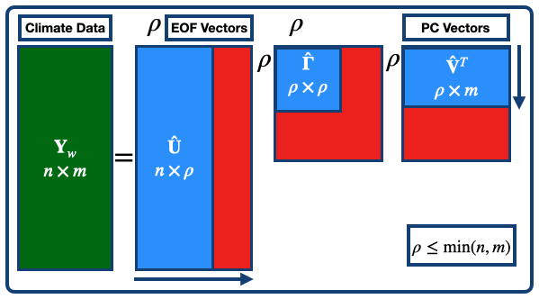
Figure 3 tSVD applied to the soil moisture anomaly dataset. The matrix Y_w(n×m) is decomposed into ${\widehat{\mathbf{U}}}_{\mathit{\rho }}(n\times \mathit{\rho })$ for EOFs, ${\widehat{\mathbf{\Gamma }}}_{\mathit{\rho }}(\mathit{\rho }\times \mathit{\rho })$ for singular values, and ${\widehat{\mathbf{V}}}_{\mathit{\rho }}^T(\mathit{\rho }\times m)$ for PCs. The truncation level ρ is chosen such that $\mathit{\rho }\le \min (n,m)$.

The singular values from tSVD are used to calculate the explained variance (%EV_i) for each EOF mode, quantifying their contribution to the dataset's variability:

$$\begin{array}{}\text{(4)}& \mathit{\%}{\mathrm{EV}}_i={\displaystyle \frac{{\mathit{\gamma }}_i}{\sum _{j=\mathrm{1}}^{\mathit{\rho }}{\mathit{\gamma }}_j}}\times \mathrm{100}\mathit{\%},i=\mathrm{1},\mathrm{2},\mathrm{\dots },\mathit{\rho }.\end{array}$$

The first EOF mode typically explains the largest fraction of variance, representing the dominant spatial pattern, while subsequent modes capture progressively smaller uncorrelated patterns. This hierarchical decomposition provides a powerful framework for analyzing spatiotemporal variability in soil moisture anomalies and assessing the relative contributions of soil hydraulic parameters and climate drivers. EOF analysis, through tSVD, ensures that the representation of dominant patterns is efficient and interpretable, enabling robust physical insights into the factors controlling soil moisture variability.

2.3.2 Quantifying similarity of spatial EOF modes using Euclidean distance

The Euclidean distance metric was employed to assess the similarity or dissimilarity between spatial EOF modes derived from distinct datasets. This metric, commonly used in mathematics and data analysis, calculates the straight-line distance between two points in Euclidean space, providing a direct and interpretable measure of the geometric proximity between patterns (e.g., Elmore and Richman, 2001). Its simplicity and intuitive interpretation make it particularly suitable for comparing spatial variability patterns obtained through EOF analysis. A smaller Euclidean distance indicates a high degree of similarity between the EOF modes, suggesting a closer similarity of the underlying spatial patterns. Conversely, a larger distance reflects greater dissimilarity, indicating distinct spatial characteristics or variability between the datasets. In this study, the Euclidean distance was used to compare the spatial EOF modes from the ERA5-Land model output and the CLM5 SP-MIP experiments, representing different data decomposition results. The Euclidean distance for two spatial EOF modes, 𝒳 (ERA5-Land) and 𝒴 (SP-MIP), was computed using the following equation:

$$\begin{array}{}\text{(5)}& \mathrm{EucD}(\mathcal{X},\mathcal{Y})=\sqrt{\sum _{i=\mathrm{1}}^n{\left({\mathcal{X}}_i-{\mathcal{Y}}_i\right)}^{\mathrm{2}}},\end{array}$$

where n is the number of spatial elements (grid points) in each EOF mode.

This approach enabled the identification of regions within the CONUS domain where the spatial EOF patterns differed significantly, highlighting areas requiring improved parameterization of soil properties in LSMs. By quantifying these differences, the Euclidean distance analysis provides actionable insights into the spatial scales and regions where soil parameter settings have the most significant impact, thereby supporting targeted model refinements and enhanced soil moisture simulations.

2.3.3 Taylor diagram for evaluating spatial EOF modes

Taylor diagrams (TDs) (Taylor, 2001) were employed to evaluate spatial EOF modes, providing a clear and intuitive representation of three key statistical measures: correlation (COR), standard deviation (STD), and root-mean-square error (RMSE). These diagrams are extensively employed in geophysical sciences to evaluate and compare model similarity across various dimensions (e.g., Qiao et al., 2022). Their ability to display, simultaneously, the relationship between modeled and reference patterns makes them particularly useful for examining the variability and accuracy of spatial EOF modes. In this research, Taylor diagrams were used to compare the spatial EOF modes of the ERA5-Land dataset against the SP-MIP model experiments. The standard deviation of the ERA5-Land spatial modes served as a reference for assessing the variability in the SP-MIP modes. The diagrams assessed the similarity of the patterns using three metrics: the correlation coefficient, which evaluates the similarity of spatial patterns; the centered RMSE, which measures the magnitude of pattern differences; and the standard deviation, which indicates the amplitude of variability within each mode. These combined metrics offer a thorough assessment of spatial pattern differences. Taylor diagrams help identify specific EOF modes where SP-MIP experiments differ from the ERA5-Land reference, pinpointing areas for possible model improvement. By incorporating these metrics into a single framework, the diagrams facilitate focused improvement of soil parameterizations in LSMs, thereby better capturing essential spatial variability patterns in soil moisture.

3 Results and discussion

3.1 Spatial variability in annual mean soil moisture across CONUS

Despite consistent forcing data (GSWP3) and model resolution (0.5°), the experiments reveal notable differences in soil moisture spatial patterns due to variations in soil parameter derivation, which underline the critical role of soil parameters in shaping simulations. These differences are reflected in the annual mean soil moisture across the CONUS region, which ranged from ≈195 to 380 kg m⁻², calculated by averaging daily soil moisture from 1980 to 2010 (Fig. 4). The spatial distribution of soil moisture across all experiments reflects well-established precipitation gradients and temperature variability, with higher soil moisture levels over the central Great Plains and ENA regions and lower values in the arid southwest. These findings align with previous studies that have documented the relationship between soil moisture, precipitation, and temperature in these regions (Welty and Zeng, 2018; Koster et al., 2004; Koukoula et al., 2021; Melillo et al., 2014; Chatterjee et al., 2022). The pronounced variability in soil moisture in the Great Plains is consistent with continentality, where greater distances from large waterbodies amplify seasonal precipitation and evaporation differences (Gimeno et al., 2010). Among the experiments, EXP3 (Fig. 4d) simulates the highest soil moisture levels, followed by EXP2 (Fig. 4c) and EXP1 (Fig. 4b). These differences reflect the impact of soil parameter treatments, with EXP1 producing lower soil moisture magnitudes, EXP2 resulting in moderate values, and EXP3 yielding the highest levels.

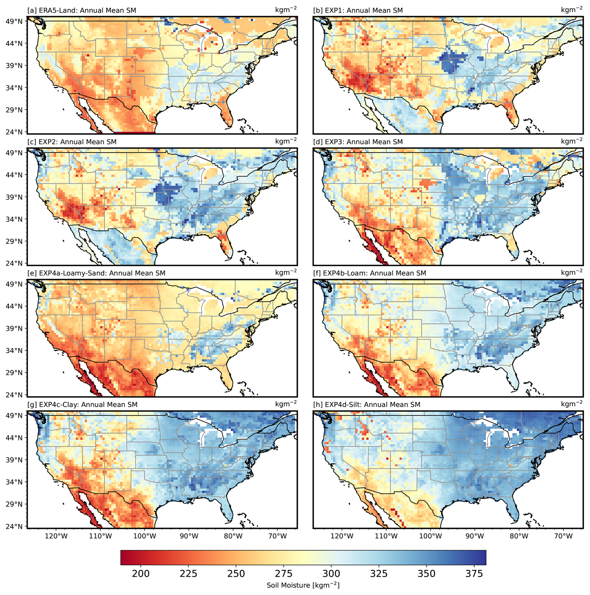
Figure 4 Annual mean soil moisture (1980 to 2010) over the CONUS region, simulated from four experiment types with differing soil parameter settings: EXP1 (b; uniform SP-MIP parameters); EXP2 (c; texture-derived, spatially varying); EXP3 (d; CLM5 defaults, spatially varying); and EXP4 – sub-experiments, including EXP4a loamy sand (e), EXP4b loam (f), EXP4c clay (g), and EXP4d silt (h), each uniform by texture class. The color bar represents the range of soil moisture values (kg m⁻²), with warmer colors (red and orange) indicating lower soil moisture levels and cooler colors (blue and purple) representing higher soil moisture levels.

The results of EXP4 highlight the role of soil texture in modulating soil moisture distribution. For example, EXP4a (loamy sand; Fig. 4e) exhibits low soil moisture in the arid southwest and NCA, consistent with the limited water retention capacity of loamy sand. EXP4b (loam; Fig. 4f) shows a more balanced soil moisture distribution, with drier conditions in WNA and wetter conditions in ENA, reflecting the moderate water-holding characteristics of the loam. EXP4c (clay; Fig. 4g) shows higher soil moisture levels over ENA due to the high water retention capacity of clay. In contrast, EXP4d (silt; Fig. 4h) exhibits heterogeneous soil moisture patterns influenced by environmental variability and the intermediate hydraulic properties of the silt. These results indicate that uncertainties in soil parameterization have a significant impact on soil moisture simulations in the CLM5 model, consistent with the findings of Brimelow et al. (2010). Our work furthers this research area by systematically evaluating the role of distinct soil textures (loamy sand, loam, clay, and silt) in shaping soil moisture variability across different climatic zones. Unlike previous studies, this analysis integrates the spatial distribution of soil moisture with climatic gradients, providing a more comprehensive assessment of how parameterization impacts hydrological processes at a continental scale. Variations in soil parameter settings not only influence soil moisture magnitudes but also alter spatial distributions, affecting the model's ability to capture hydrological processes at the continental scale. The findings of EXP4 further emphasize the importance of soil texture in controlling the soil moisture distribution, highlighting the need for precise parameterization in LSMs. This has important implications for improving water resource management, agricultural planning, and climate impact assessments.

3.2 Interannual soil moisture anomalies

Interannual root-zone soil moisture anomalies over the CONUS region from 1980 to 2010, derived from CLM5 simulation experiments (EXP1, EXP2, EXP3, and multiple EXP4 configurations) and ERA5-Land model output (model-based pattern reference), are shown in Fig. 5. Anomalies are computed as deviations from the daily annual mean over the 30-year reference period, following established methodologies for hydrological variability assessment (Tuttle and Salvucci, 2016; Koster et al., 2004; Welty and Zeng, 2018). The top panel of Fig. 5 presents anomalies for EXP1, EXP2, EXP3, and ERA5-Land, while the bottom panel includes additional EXP4 parameterizations representing different soil textures (loamy sand, loam, clay, and silt).

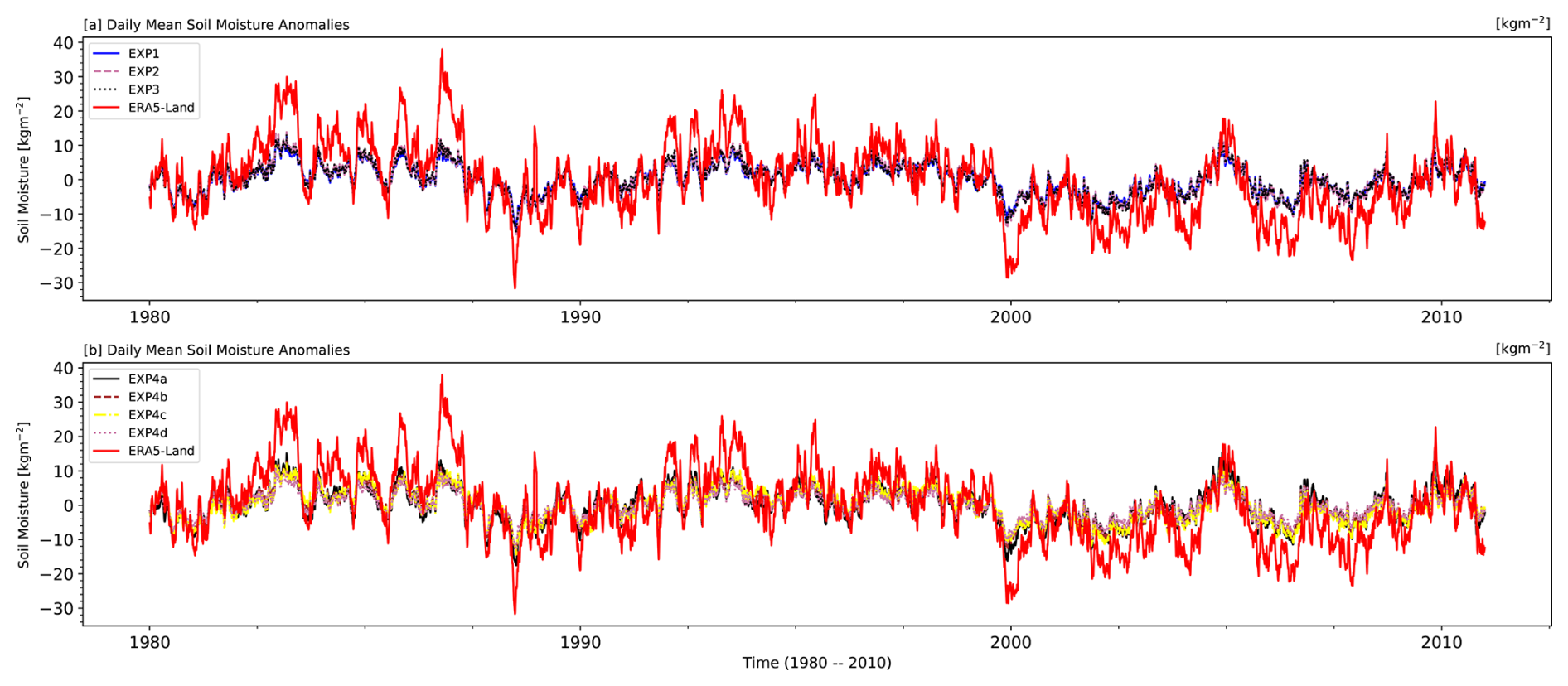
Figure 5 Time series of daily root-zone soil moisture anomalies from 1980 to 2010 over the CONUS region. Panel (a) displays anomalies for CLM5 simulations using EXP1, EXP2, and EXP3 configurations, compared with ERA5-Land (the model-based pattern reference). Panel (b) includes EXP4 simulations with uniform soil texture classes (loamy sand, loam, clay, and silt), also compared against ERA5-Land. Anomalies are computed as deviations from the 30-year daily climatological mean. ERA5-Land exhibits a wider anomaly range, while CLM5 simulations show more constrained variability, highlighting differences in interannual amplitude across configurations.

Across all configurations, soil moisture anomalies fluctuate around a long-term mean of zero, with values ranging approximately from −20 to +40 kg m⁻². Positive anomalies signify wetter-than-average conditions, while negative values indicate drier conditions. The CLM5 experiments exhibit pronounced interannual variability, capturing key hydrological extremes, including droughts and wet periods, as represented in ERA5-Land patterns. CLM5 simulations reproduce the timing of major interannual features present in ERA5-Land patterns, such as drought and wet periods, but consistently underestimate their magnitude. As shown in Fig. 5, all CLM5 configurations produce tightly clustered time series, lacking the broader spread in ERA5-Land. This visual clustering illustrates a key discrepancy: ERA5-Land exhibits a broader interannual amplitude, with anomalies reaching up to ±40 kg m⁻², whereas CLM5 simulations are typically confined to a ±20 kg m⁻² range; note that differences can also reflect forcing and structural contrasts (GSWP3-forced CLM5 vs. ERA5-forced HTESSEL in ERA5-Land) in addition to parameter effects.

This variability gap likely stems from structural limitations in CLM5, including the use of static soil hydraulic parameters, diffusive vertical redistribution, and the absence of data assimilation factors known to constrain the dynamic range and persistence of soil moisture anomalies in LSMs (Koster et al., 2009; Muñoz-Sabater et al., 2021). The underestimation is particularly concerning for hydrologic extremes, as it suggests that CLM5 may inadequately simulate the severity of soil moisture deficits during droughts or surpluses during wet years. These limitations can propagate into downstream processes such as evapotranspiration, runoff, and land–atmosphere coupling, thereby reducing the model's ability to capture feedback mechanisms critical to hydroclimatic variability (Koster et al., 2004; Berg and Sheffield, 2018). Figure 6 supports this interpretation, showing that CLM5 anomaly values are compressed along the 1:1 line when compared to ERA5-Land, reinforcing the conclusion that the model's soil moisture response is systematically dampened. Finally, while ERA5-Land's higher peaks – particularly in positive extremes – may partly reflect an overestimation in vegetated regions due to unresolved processes such as irrigation or enhanced surface fluxes (Lal et al., 2022), the muted variability in CLM5 indicates the importance of improved parameter calibration and multi-source reference datasets in future work.

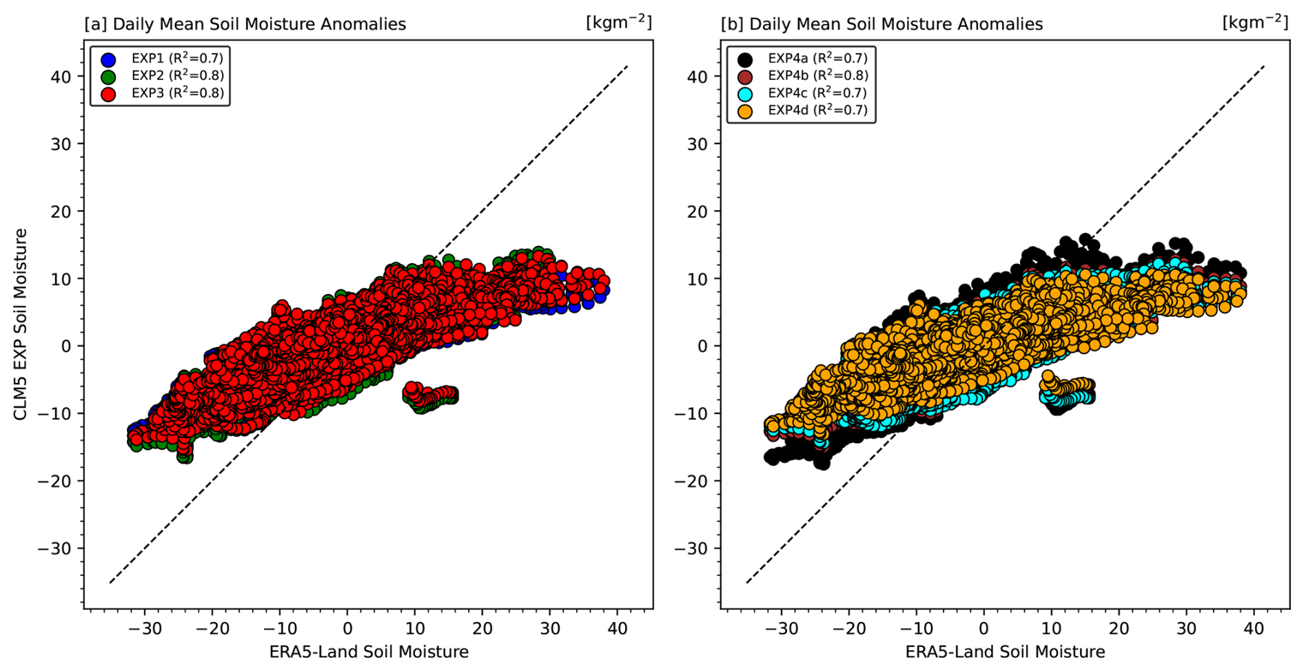
Figure 6 Daily mean root-zone soil moisture anomalies for 1980 to 2010 from each CLM5 experiment (EXP1, EXP2, EXP3, and the EXP4 sub-experiments) plotted against ERA5-Land (model-based pattern reference). All anomalies are expressed in kilograms per square meter (kg m⁻²). Each colored marker represents daily anomalies from a given experiment, while the dashed black line denotes the 1:1 relationship. In the legend, R² values (in parentheses) indicate the degree to which each experiment's anomalies align with ERA5-Land patterns.

The relationship between daily soil moisture anomalies from CLM5 and ERA5-Land is further examined in Fig. 6. These scatterplots compare CLM5-simulated anomalies with ERA5-Land on a point-by-point basis. The distribution of points is closely aligned along the 1:1 line, with coefficient of determination (R²) values ranging from 0.7 to 0.8 across experiments. These correlations confirm that CLM5 successfully captures much of the variability present in ERA5-Land patterns, albeit with some systematic biases. Specifically, ERA5-Land tends to exhibit larger positive anomalies relative to CLM5, reinforcing the trend seen in the time-series plots. The EXP4 configurations (Fig. 6b) show similarity to EXP1–EXP3, indicating that soil texture variations only moderately impact anomaly correlations at an aggregated scale.

The results indicate significant interannual variability in soil moisture anomalies, with distinct peaks and troughs corresponding to extreme hydrological events. These fluctuations are likely driven by large-scale climatic influences, such as ENSO, which modulate regional hydrological conditions (Gimeno et al., 2010; Welty and Zeng, 2018). While periodicity in anomalies suggests a possible linkage to climate oscillations, further spectral analysis would be required to confirm such relationships. Additionally, the lack of a discernible long-term trend indicates that soil moisture anomalies remained relatively stable over the study period, with variability largely governed by short- to medium-term hydrological cycles. This aligns with findings from Lesinger and Tian (2022), who noted that, while interannual fluctuations in soil moisture can be significant, multi-decadal trends over CONUS tend to be weak or spatially constrained. Overall, the time series (Fig. 5) and scatterplots (Fig. 6) collectively demonstrate that CLM5 reasonably captures the timing and structure of interannual soil moisture variability, but it consistently underestimates its magnitude relative to ERA5-Land patterns, with strong correlations. However, ERA5-Land's systematic overestimation of positive anomalies indicates a potential bias in reanalysis products, necessitating further evaluation of the mechanisms driving such deviations. Accordingly, we interpret the ERA5-Land comparison strictly as a pattern-based reference. Similarities indicate that CLM5's parameter choices reproduce timing, phase, and spatial covariance seen in an independent model product, whereas systematic departures highlight parameter-sensitive regions; neither case is taken as validation of absolute soil moisture levels. Future work should assess regional patterns in soil moisture dynamics and quantify biases across different land cover types to improve pattern similarity.

3.3 Seasonal variability in soil moisture

As evident in Fig. 7, notable differences emerge between ERA5-Land patterns (model-based pattern reference) and CLM5 simulations, particularly with respect to the amplitude of seasonal variability. ERA5-Land exhibits the strongest seasonal cycle, with a sharp rise in soil moisture from February through May, peaking in June, followed by a pronounced decline into the late-summer and early-autumn months. In contrast, EXP1, EXP2, and EXP3 form a tightly clustered group with relatively flattened seasonal curves. These configurations consistently underestimate the springtime peak and summer drawdown, suggesting that their soil moisture response to seasonal climate forcing is muted. Among them, EXP2 (green line) shows the lowest amplitude, while EXP3 (red line) offers a slightly improved but still subdued representation.

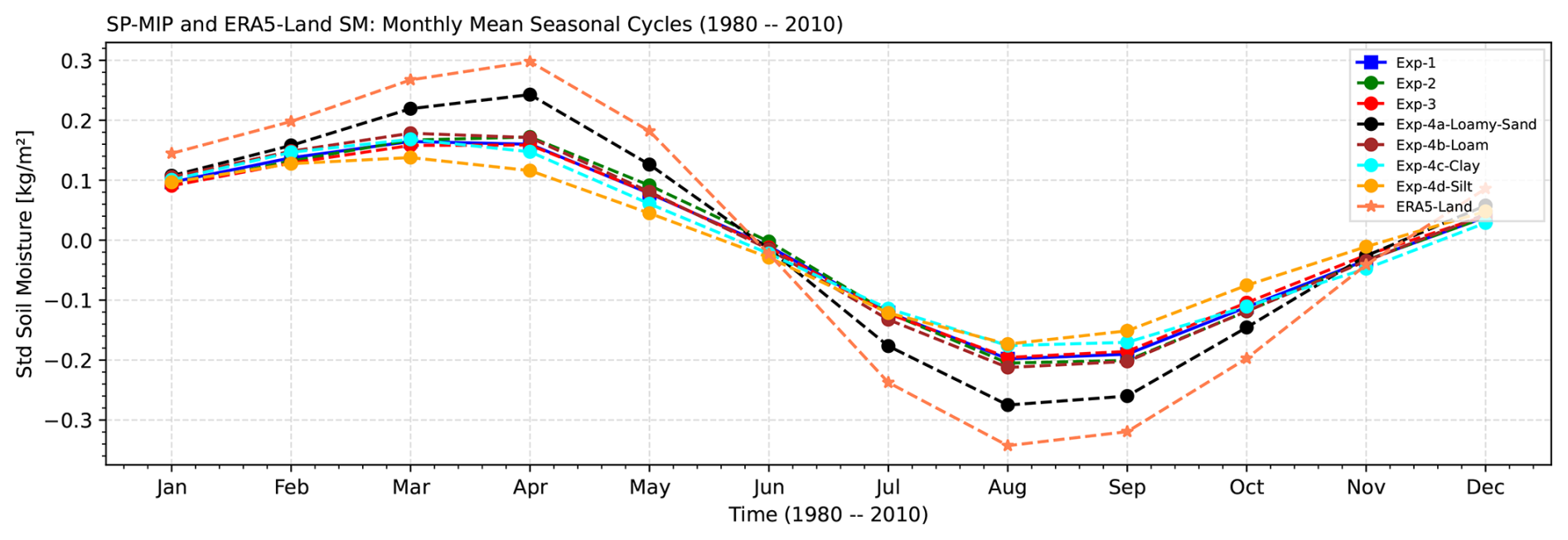
Figure 7 Monthly mean seasonal cycles of standardized root-zone soil moisture for the period from 1980 to 2010 across the CONUS. CLM5 simulations (EXP1–EXP3 and EXP4a–EXP4d) are compared with ERA5-Land (model-based pattern reference). ERA5-Land exhibits the largest seasonal amplitude, with sharp increases during spring (March–June) and steep declines during summer (July–October). In contrast, EXP1–EXP3 form a tightly clustered group with flattened seasonal cycles, underestimating both the spring moisture accumulation and summer drawdown. EXP4a, which uses a loamy sand texture, shows greater seasonal responsiveness and greater similarity to ERA5-Land seasonal patterns. The remaining EXP4 configurations (loam, clay, and silt) progressively dampen seasonal variability, reflecting the influence of soil texture on water retention and hydrologic dynamics.

Notably, EXP4a (dashed black line) deviates from this pattern. It shows greater similarity to ERA5-Land seasonal patterns, especially from March to September, capturing a steeper ascent in spring and a deeper trough in late summer. This improved responsiveness is likely due to the loamy sand texture used in EXP4a, which promotes rapid infiltration and drainage, thereby amplifying soil moisture variability in response to precipitation and evapotranspiration. In contrast, EXP4b–d (loam, clay, and silt) progressively dampen the seasonal signal, with EXP4c and EXP4d showing the lowest variability due to their high water retention capacities.

These differences indicate that, while it reproduces the general phasing of the seasonal cycle, CLM5 substantially underrepresents the amplitude of variation in ERA5-Land patterns. This underestimation is especially critical during the peak moisture accumulation (March–June) and depletion (July–October) phases, and it highlights the importance of hydraulic conductivity, retention characteristics, and vertical redistribution in modulating soil moisture seasonality. Although ERA5-Land may overestimate soil moisture in certain vegetated regions (Lal et al., 2022; Lesinger and Tian, 2022), its higher amplitude suggests a more dynamic land surface response that current CLM5 configurations, particularly EXP1–EXP3, fail to capture adequately. Addressing this discrepancy through improved parameter tuning and structural adjustments could enhance CLM5's ability to simulate land–atmosphere coupling and surface hydrological processes across seasons.

3.4 EOF analysis of soil moisture variability

3.4.1 Explained variance and mode contributions

This study applies EOF analysis to soil moisture anomalies from the CLM5 simulations (EXP1, EXP2, and EXP3) and the ERA5-Land model output (model-based pattern reference, with no soil moisture assimilation and no ground truth) to investigate how soil parameterization influences soil moisture variability in the CONUS region. Figure 8 presents the percentage of variance explained by the first 10 EOF modes for each dataset, illustrating both individual and cumulative contributions. The EOF modes are ranked by variance percentage, with EOF-1 capturing the highest variance and representing the most significant spatial variability. Across all experiments, EOF-1 explains slightly more variance than EOF-2, suggesting limited separation between these modes and potential mode mixing. The explained variance gradually declines in subsequent modes, with EOF-10 contributing less than 2 %, as summarized in Table 4. EOF-1 explains a similar percentage of variance in EXP1 (11.45 %) and EXP2 (11.66 %), indicating comparable spatial variability patterns. However, in EXP3, EOF-1 captures only 10.84 % of the variance, with mode mixing shifting variance from EOF-1 to EOF-2 (Table 3, arrows). These differences highlight the impact of soil parameterization on representing dominant soil moisture variability. ERA5-Land, used here as a pattern reference, exhibits a larger EOF-1 contribution (17.5 %), indicating a more dominant leading mode than in the CLM5 runs; differences can also reflect forcing (ERA5 vs. GSWP3) and structural (HTESSEL vs. CLM5) contrasts, not parameter effects alone. The cumulative explained variance (Fig. 8, green line) shows how efficiently the leading modes summarize variability in each dataset.

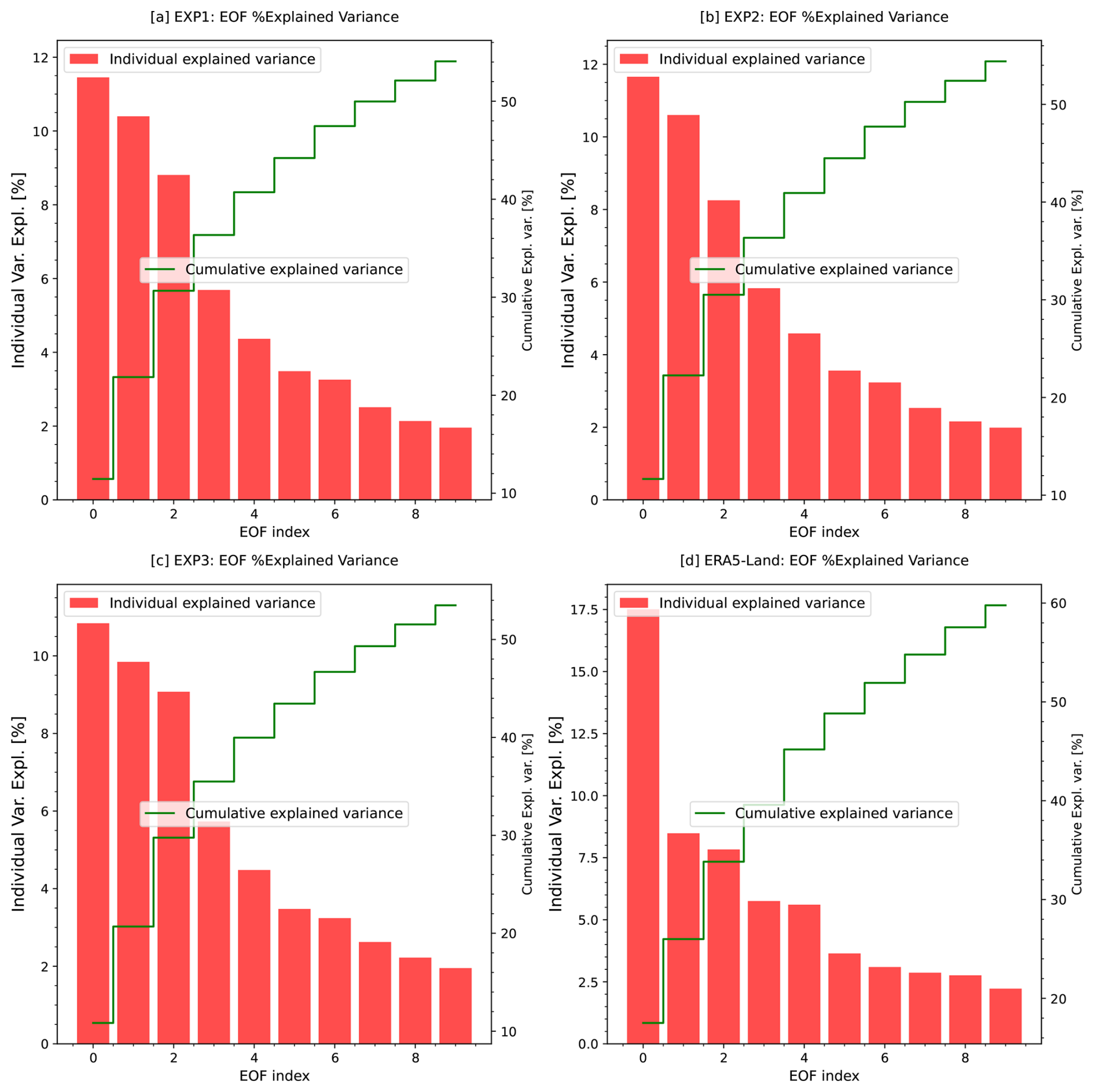
Figure 8 The variance explained by each EOF (red bars); the cumulative variance (green line) shows the cumulative proportion for the initial 10 EOF modes.

Table 4 Percentage of variance explained (%Expl. Var.) by the first 10 EOF modes for the EXP1, EXP2, and EXP3 model runs and for ERA5-Land reference data. Arrows and superscripts indicate EOF mode swaps (flagged in bold) for consistent comparisons across datasets (see Fig. 9).

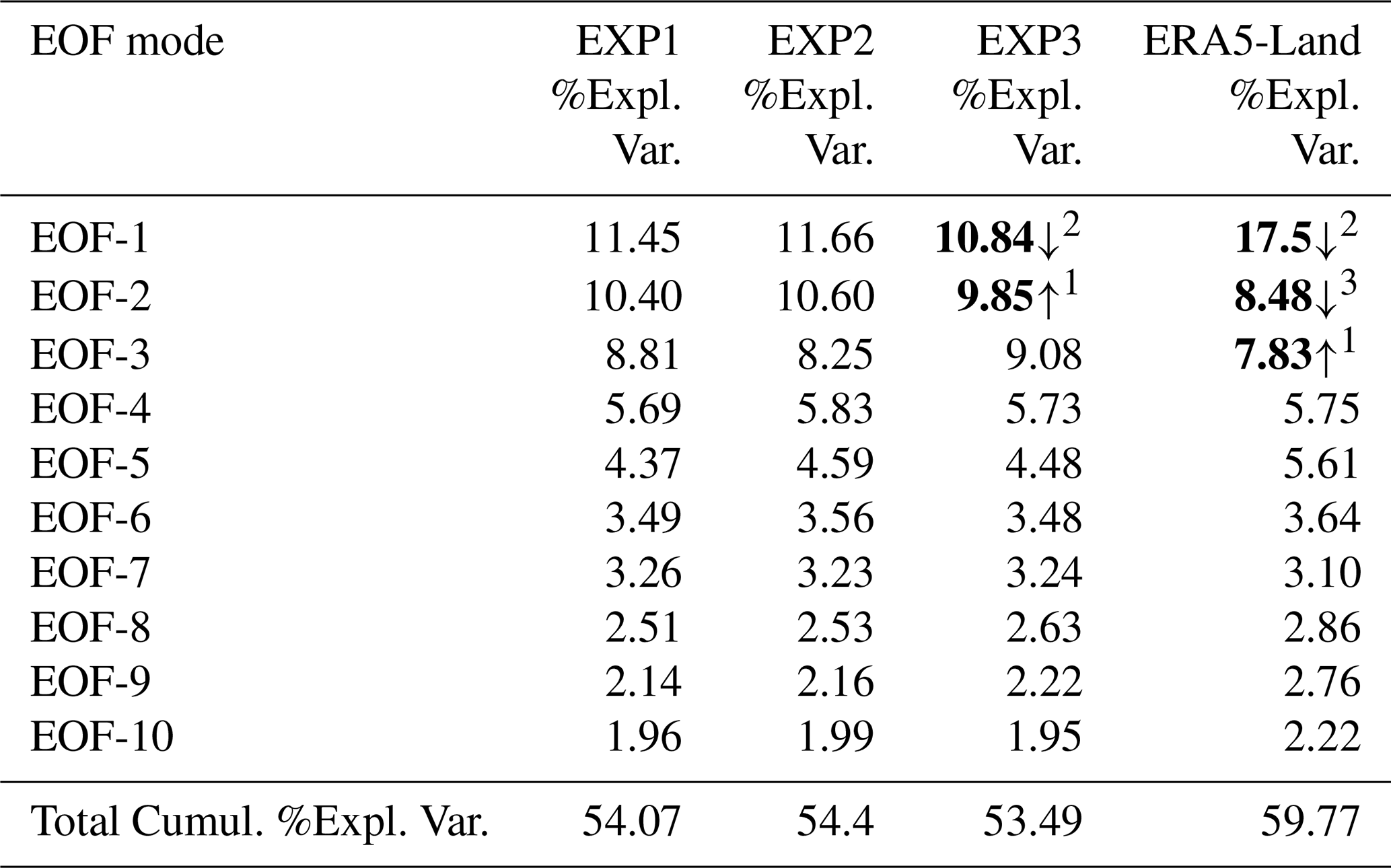
While the first five modes account for about 40 % of the variance in ERA5-Land, the CLM5 simulations require approximately six modes to reach the same threshold. This distribution suggests that the simulations spread variance more evenly across modes, reflecting differences in spatial patterns between CLM5 simulations and ERA5-Land. To facilitate cross-dataset comparison, we re-ordered EOF modes where necessary so that the dominant spatial patterns were aligned across datasets. For instance, shifts in EXP3 and ERA5-Land were necessary to match the dominant spatial patterns, such as the swaps of EOF-1 and EOF-2 (indicated by arrows in Table 3). These adjustments highlight the sensitivity of EOF rankings to mode mixing and the challenges of directly comparing different model products (CLM5 and ERA5-Land). In addition, Appendix A (Fig. A1) provides additional EOF analysis results for EXP4a–EXP4d, detailing variance explained across experiments. The findings reinforce the influence of soil parameterization on the spatial distribution of soil moisture, emphasizing that comparisons are interpreted in terms of similarity to ERA5-Land patterns rather than validation of absolute levels.

3.4.2 Spatial and temporal analysis of EOF modes for soil moisture variability

We show the spatial distribution of the first three EOF modes from soil moisture anomalies in CLM5 simulations (EXP1, EXP2, and EXP3) and ERA5-Land (model-based pattern reference). The maps in Fig. 9 show correlation coefficients between the PC time series of each EOF mode and the soil moisture anomaly time series at each grid point. These correlation maps indicate the spatial strength and direction of the association between local anomalies and the broader temporal mode represented by the PC. This representation facilitates interpretation by highlighting regions that co-vary in phase (positive correlation) or in antiphase (negative correlation) with the dominant temporal pattern, thereby revealing the spatial structure of soil moisture variability linked to each EOF mode. EOF-1 patterns (Fig. 9d, g, and j) reveal strong positive correlations in central and southeastern ENA, highlighting a dominant mode of variability. Negative correlations are seen in WNA and CNA, indicating contrasting modes of soil moisture variability in the CONUS region. The variance explained by EOF-1 ranges from 9.85 % (EXP3) to 11.66 % (EXP2), with ERA5-Land showing a larger variance contribution (17.5 %). These spatial patterns align with large-scale climatic influences, such as precipitation and temperature gradients, as well as geographic features. For example, Gaffin and Hotz (2000) noted that the Appalachian Mountains exhibit strong precipitation gradients due to storm systems lifting moist southerly winds, enhancing soil moisture in ENA. The corresponding principal components (PC-1; Fig. 10a) indicate temporal variability, with notable peaks during 2003–2004 and 1988–1999, corresponding to documented climatic events such as ENSO-driven precipitation anomalies (Ye et al., 2023; Gimeno et al., 2010). The close agreement of PC-1 across all experiments indicates the robustness of EOF-1 in representing the dominant variability in soil moisture, although slight differences suggest some sensitivity to parameterizations.

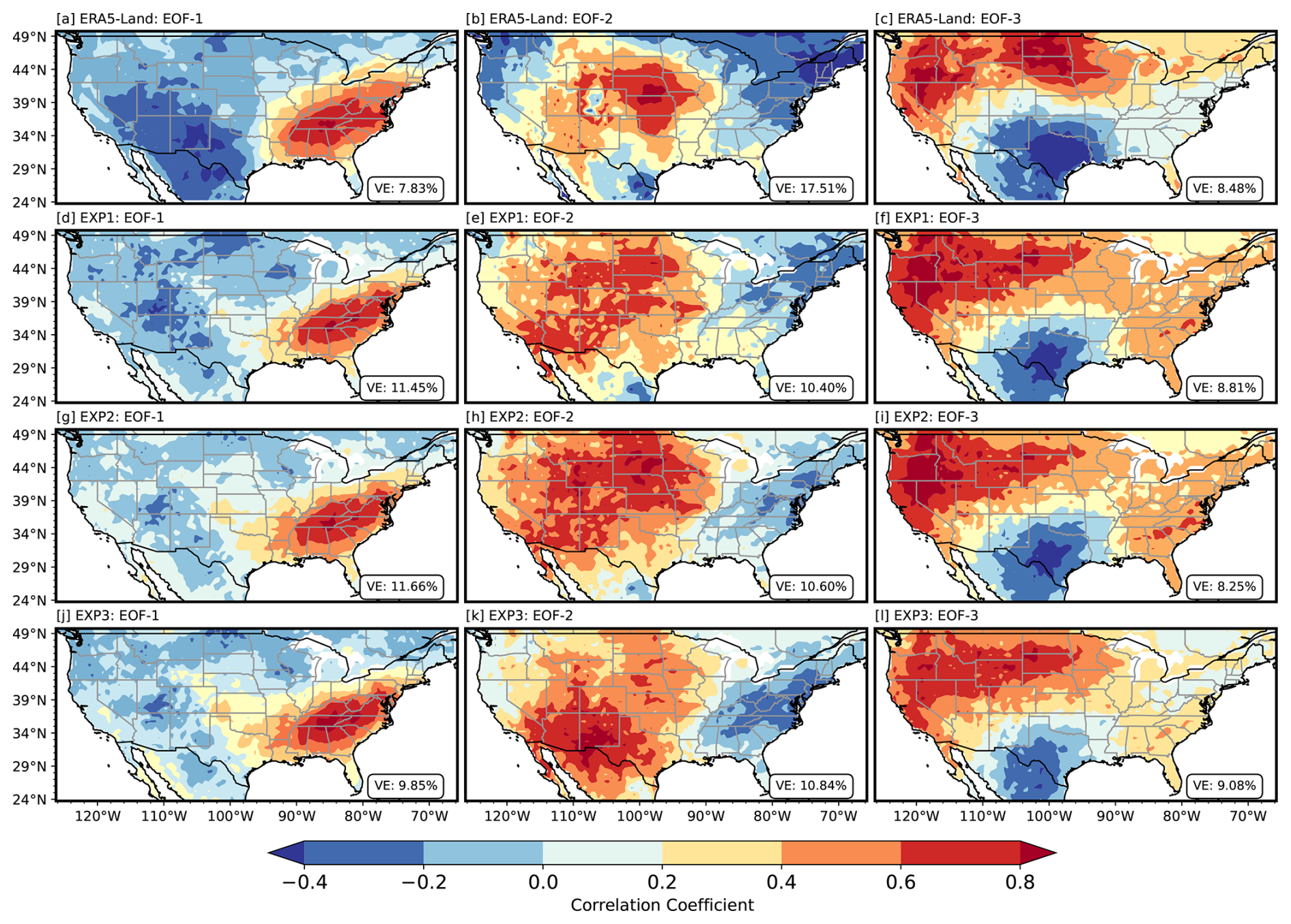
Figure 9 Spatial correlation maps of the first three EOFs of soil moisture anomalies for the CONUS region, derived from ERA5-Land (model-based pattern reference) and three CLM5 experiments (EXP1, EXP2, and EXP3). Panels (a) to (c) represent EOF-1, EOF-2, and EOF-3 from ERA5-Land, respectively. Panels (d)–(f), (g)–(i), and (j)–(l) show corresponding modes from EXP1, EXP2, and EXP3. The colored shading represents the correlation coefficient between the PC time series of each EOF mode and the soil moisture anomaly time series at each grid point. Positive values indicate in-phase variability with the PC (regions that co-vary with the dominant mode), while negative values indicate antiphase behavior. These maps illustrate the spatial coherence and phase relationships of soil moisture variability associated with each mode.

EOF-2 (Fig. 9e, h, and k) exhibits a distinct dipole pattern, with positive correlations in the central Great Plains and negative correlations over ENA, reflecting a wide spread in soil moisture variability. This dipole nature, which explains 10.40 % to 10.84 % of the variance, is consistent with regional climatic processes such as precipitation and evapotranspiration dynamics influenced by terrain and hydrological conditions. For example, positive correlations in the central Great Plains may result from localized convective precipitation; however, isotope studies indicate that precipitation in this region is influenced by moisture transported from external sources, such as the Gulf of Mexico, rather than solely from local convection (Sanchez-Murillo et al., 2023). Negative correlations in ENA could reflect the influence of evapotranspiration or soil drainage patterns (Famiglietti, 2014). In particular, EXP3 exhibits a stronger positive correlation in the desert southwest, suggesting a greater sensitivity to soil parameters in arid regions, which can influence soil water retention and infiltration rates. Furthermore, EOF-3 (Fig. 9f, i, and l) highlights localized variability, with positive correlations in the Pacific Northwest and negative correlations over Texas in CNA. This mode explains less variance than EOF-1 and EOF-2 (8.25 % in EXP2 to 9.8 % in EXP3) but captures important regional processes. The Pacific Northwest patterns may be influenced by orographic precipitation. At the same time, negative correlations in Texas could reflect drought conditions and the influence of fine-textured soils with higher water-retention potential (Haverkamp et al., 2005). Although the spatial patterns of EOF-3 are broadly similar between experiments, slight shifts in correlation intensity and location suggest localized impacts of soil parameterizations. The PCs (Fig. 10c) show weaker temporal variability with occasional peaks tied to distinct climate events, emphasizing the regional specificity of EOF-3. The Appendix includes Figs. A2 and A3, which offer additional results highlighting the spatial and temporal variability in the EXP4a–EXP4d EOFs across experiments, further supporting the findings discussed. Lastly, the results emphasize the significant role that soil parameterizations play in soil moisture variability within the CLM5 model. Differences in the spatial and temporal patterns of EOFs indicate the model's sensitivity to these parameterizations, especially in areas with intricate terrain or significant climate variability. The greater similarity of EOF-1 to ERA5-Land patterns underlines the robustness of the model's primary modes, while discrepancies in EOF-2 and EOF-3 highlight regions where model refinements could enhance localized soil moisture predictions. This study stresses the importance of improving soil parameterizations to improve the representation of hydrological variability and effectively capture the interaction between soil moisture and climatic elements.

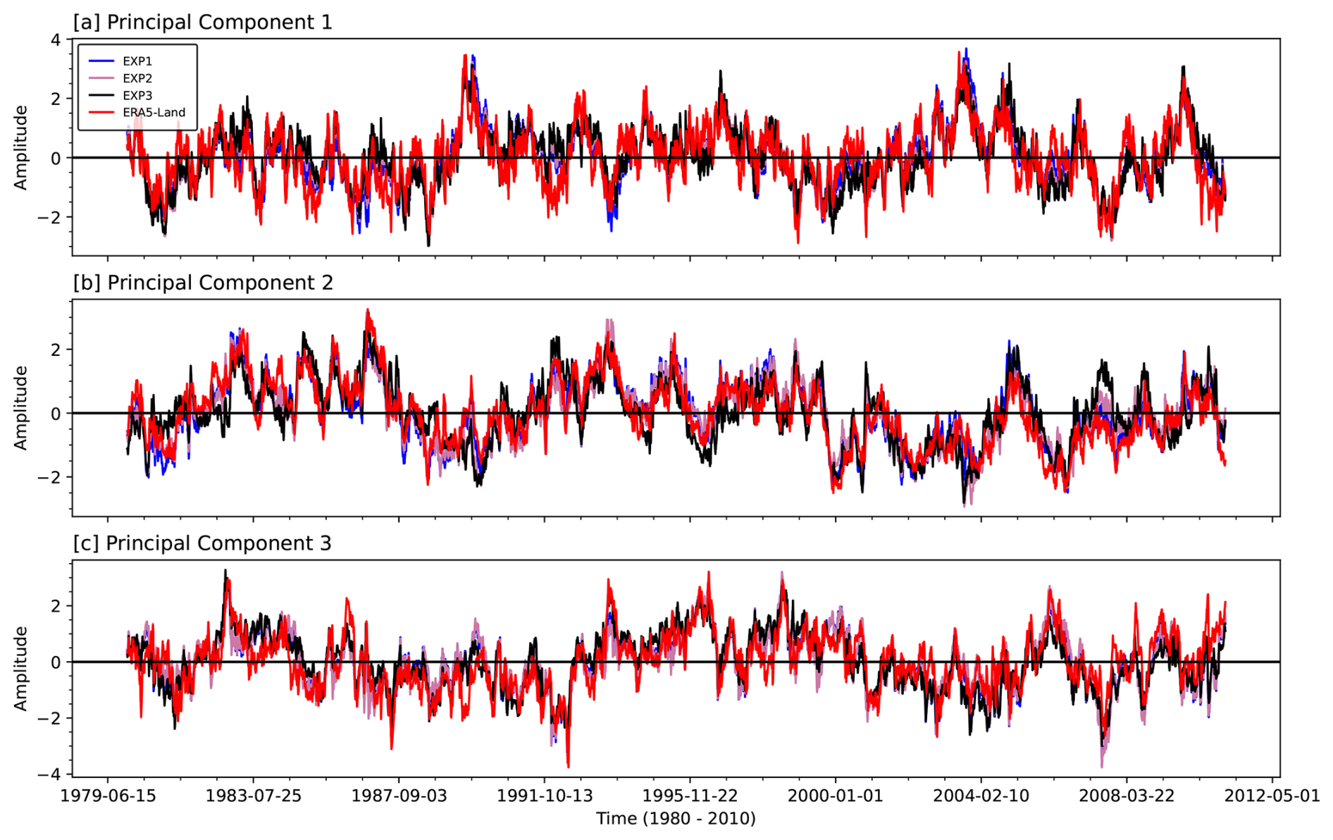
Figure 10 Temporal variability (PC) in corresponding EOFs over time (1980–2010) displaying the amplitude of the first four PCs: EXP1 (blue), EXP2 (green), and EXP3 (orange) derived from the soil moisture decomposition for each simulation experiment.

3.4.3 EOF modes: Euclidean distance analysis

We compute the Euclidean distance (Fig. 11) between the spatial patterns of EOF modes derived from soil moisture anomalies in the CLM5 SP-MIP experiments (EXP1, EXP2, and EXP3) and the corresponding modes from ERA5-Land model output (model-based pattern reference; not the ground truth). Euclidean distance quantifies dissimilarity between spatial modes, with smaller values indicating greater similarity to ERA5-Land patterns. Regions with hatched lines denote areas where the distance falls below a threshold of 5, suggesting strong pattern similarity between the CLM5-derived EOFs and the ERA5-Land EOFs. EOF-1 (Fig. 11a, d, g) exhibits the most consistent similarity across experiments, particularly in the western and northwestern CONUS (WNA). The hatched areas there indicate that the modeled spatial variability shows close similarity to ERA5-Land patterns, consistent with large-scale hydrologic controls such as precipitation gradients and topography (Gaffin and Hotz, 2000; Famiglietti, 2014). In contrast, the central Great Plains consistently shows larger Euclidean distances for all three EOF modes, indicating notable pattern differences between CLM5 and ERA5-Land in this region. These differences may reflect limitations in soil parameterizations and the complexity of hydroclimatic processes (e.g., precipitation variability and soil moisture–precipitation feedbacks) (Koster et al., 2004; Welty and Zeng, 2018), as well as forcing and structural contrasts between datasets (CLM5 forced by GSWP3 vs. ERA5-Land as an offline HTESSEL replay forced by ERA5). Relative to ERA5-Land patterns, EXP1 shows greater similarity in WNA for EOF-1, while similarity in other regions is mixed across experiments. EOF-2 (Fig. 11e, d, h) and EOF-3 (Fig. 11c, f, i) display larger distances with fewer hatched areas, indicating challenges with respect to capturing smaller-scale structures and dipole patterns (Hannachi et al., 2007; Monahan et al., 2009). These findings underline the model's sensitivity to soil parameter choices and highlight the need for targeted improvements in the central Great Plains and other regions with persistent pattern differences. Refining soil parameter settings and incorporating independent datasets (e.g., SMAP, in situ networks) as complementary references could help improve the representation of regional soil moisture patterns.

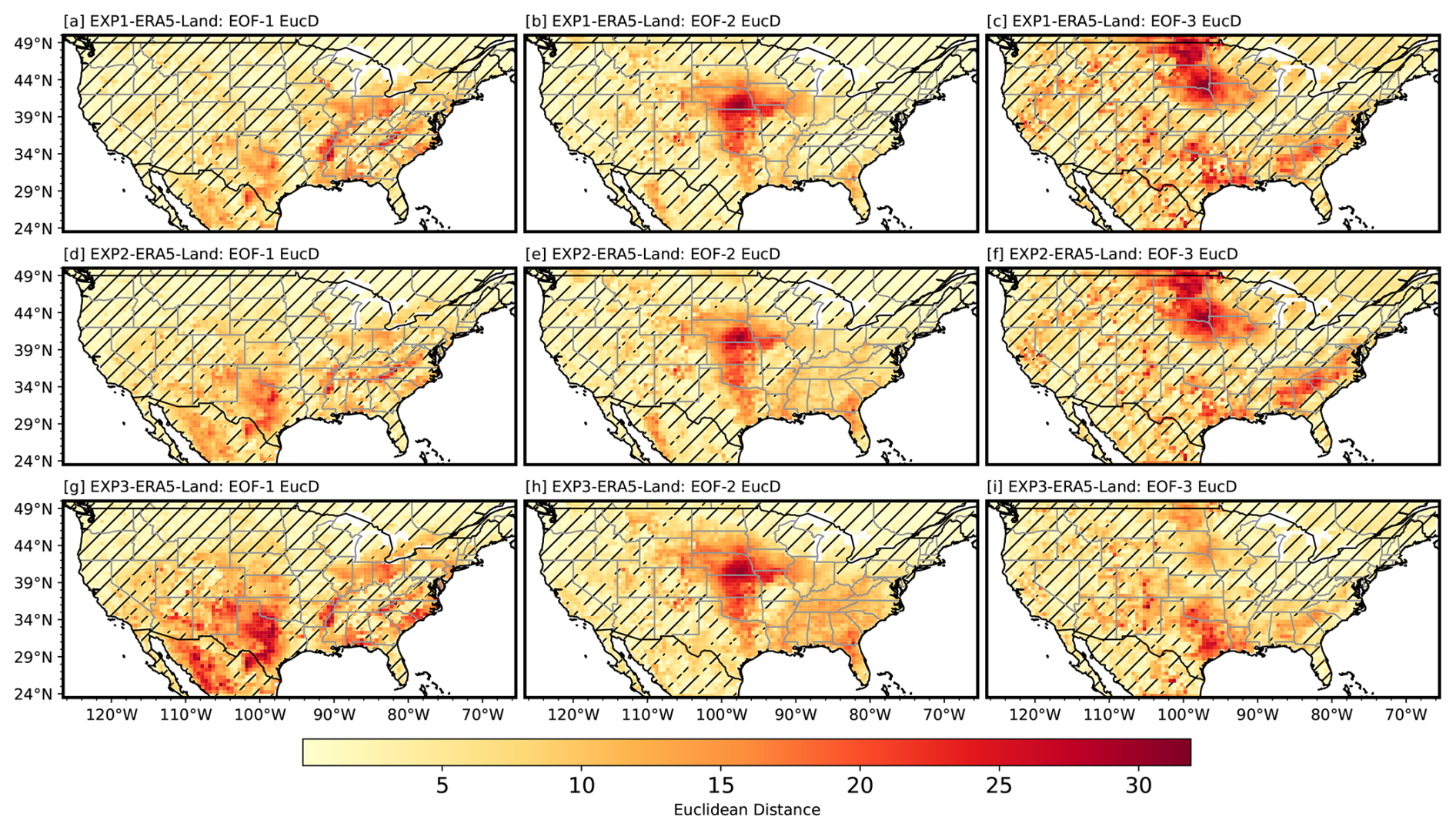
Figure 11 Euclidean distance between EOF modes from SP-MIP experiments (EXP1, EXP2, and EXP3) and ERA5-Land (model-based pattern reference). Hatched areas indicate regions where the distance is below 5, indicating greater similarity to ERA5-Land patterns.

3.4.4 EOF modes: Taylor diagram analysis

TDs (Fig. 12) summarize the similarity of EOF patterns from different experiments to those in ERA5-Land (model-based pattern reference) using three statistics: standard deviation (dotted arcs), correlation coefficient, and centered root-mean-square error (RMSE). Each marker's position indicates the degree of pattern similarity between a modeled EOF mode and the ERA5-Land EOF mode. For EOF-1 (Fig. 12a), the standard deviations of the EOF modes for all model experiments are relatively close to the reference EOF mode, ranging between 4.0 and 6.5, which suggests close similarity in variability. The pattern correlations range between 0.6 and 0.95, with EXP4d demonstrating the highest pattern correlation. This indicates that the spatial pattern of EXP4d shows greater similarity to the ERA5-Land EOF mode. In EOF-2 (Fig. 12b), the standard deviations are comparable to the reference EOF mode, while pattern correlations cluster between 0.4 and 0.7, indicating moderate similarity for the second mode. For EOF-3 (Fig. 12c), the EOF modes generally exhibit a pattern correlation of around 0.8 and a standard deviation of approximately 5.0. However, the EXP4d EOF deviates, centered around a lower standard deviation of 3.5. These variations highlight the impact of soil parameter settings in CLM5, demonstrating how parameter choices influence the similarity to ERA5-Land EOF patterns.

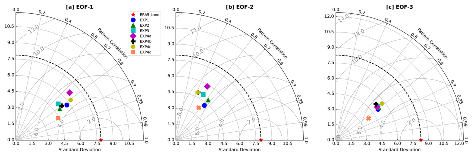
Figure 12 Taylor diagrams (TDs) for the leading three EOFs from multiple experiments (EXP1, EXP2, EXP3, EXP4a, EXP4b, EXP4c, and EXP4d) and ERA5-Land. The diagrams summarize the standard deviation, correlation coefficient, and RMSE, with marker placement indicating pattern similarity relative to ERA5-Land (model-based pattern reference).

4 Conclusion and recommendations

This study examines the impact of soil parameterizations on soil moisture simulations in the CLM5 across the CONUS for the period from 1980 to 2010, utilizing EOF analysis. We compared CLM5 simulations to ERA5-Land, used solely as a model-based pattern reference, and quantified the similarity of spatial and temporal patterns across soil parameter configurations. The results showed that EXP3, which used the default CLM5 soil parameters, consistently simulated higher soil moisture levels than other experiments. This finding highlights the model's sensitivity to variations in soil hydraulic properties, including saturated hydraulic conductivity, soil water retention characteristics, and porosity. Seasonal soil moisture dynamics showed broad consistency across experiments, peaking in winter due to reduced evapotranspiration, and declining in summer, when higher temperatures intensified soil drying. However, distinct differences emerged in the magnitude and phase of seasonal cycles, revealing how variations in soil properties can influence processes such as water retention, drainage, and evapotranspiration fluxes. These insights align with previous research, which demonstrated that soil moisture significantly affects hydrological processes and land–atmosphere interactions, particularly through feedback mechanisms that vary regionally across the United States (Tuttle and Salvucci, 2016; Koster et al., 2004). Furthermore, the amplified sensitivity seen in the arid and semiarid regions of the CONUS suggests that these areas may be particularly vulnerable to uncertainties in soil parameterization.

Regarding the first question, EOF analysis revealed that changes in soil hydraulic properties significantly altered the spatial distribution of the dominant EOF modes, particularly in regions such as the Great Plains and ENA, indicating that parameterizations strongly influence modeled soil moisture gradients. For the second question, principal component time series associated with the leading EOFs captured interannual anomalies and periods of extreme wetness or dryness that coincided with known climate events (e.g., ENSO phases). Variations in the amplitude and persistence of these temporal patterns across experiments underlined the role of soil parameters in modulating the hydrologic response to climate variability. These findings affirm that parameter choice not only controls spatial representation but also influences the sensitivity of soil moisture to climatic extremes, highlighting the dual spatial–temporal impact of soil parameterization in land surface modeling.

EOF analysis further revealed that the first few modes accounted for most of the variance across experiments, and EOF-1 consistently explained the most significant proportion of variance. The spatial patterns of the first three EOF modes exhibited similar broad-scale features among the experiments, such as dominant moisture gradients across climatic zones. However, notable differences in explained variance and spatial correlations pointed to the influence of soil parameters on the physical processes driving regional moisture variability. Compared with ERA5-Land patterns using Euclidean distances and Taylor diagrams, the CLM5 output showed greater similarity in WNA, indicating closer correspondence to ERA5-Land's representation of mountainous and arid region dynamics. In contrast, persistent discrepancies in the central Great Plains revealed challenges with respect to representing complex interactions between soil hydraulic properties, precipitation variability, and surface–atmosphere feedbacks. These discrepancies are particularly concerning given the region's susceptibility to extreme hydrological events, including droughts and floods (Koster et al., 2004; Ye et al., 2023). The Great Plains is characterized by a highly variable continental climate, with strong seasonal and interannual fluctuations in precipitation and temperature, leading to frequent shifts between wet and dry extremes (Basara and Christian, 2018; McDonough et al., 2020). This climatic variability makes the region hydrologically complex, requiring an accurate representation of soil moisture dynamics for land surface hydrology modeling. Errors in soil moisture estimation can propagate into predictions of crop productivity, water resource availability, and flood risk. The findings suggest that refining soil hydraulic parameterizations, such as incorporating high-resolution soil texture data and accounting for heterogeneity, can significantly improve the predictive capacity of CLM5 and other LSMs for climate studies, ecosystem assessments, and resource management. While our comparative framework assessed the aggregate effects of parameter set differences, we did not perform a formal sensitivity analysis to isolate the influence of individual soil hydraulic properties (e.g., saturated hydraulic conductivity, porosity, and van Genuchten parameters), which remains an important area for future investigation.

This study is an intra-model sensitivity analysis; all comparisons are model-to-model and pattern-based, not validations against observations. We use ERA5-Land only as a spatially complete, temporally consistent, model-based pattern reference to gauge the similarity of CLM5 spatial and temporal modes; it does not assimilate soil moisture observations and shows documented regional biases (e.g., wet bias in humid and vegetated areas), so it is not the ground truth (Muñoz-Sabater et al., 2021; Wu et al., 2021; Zhang et al., 2023). Forcing and structural mismatches also limit attribution: CLM5 is forced by GSWP3, whereas ERA5-Land is an offline HTESSEL replay forced by ERA5, so differences can reflect forcing and model-structure contrasts in addition to parameter effects. We chose ERA5-Land because it provides CONUS-wide coverage at a resolution compatible with CLM5 (after regridding to 0.5^∘) and exhibits coherent seasonal–interannual variability that aligns with our pattern-oriented objectives. Finally, neither CLM5 nor ERA5-Land includes irrigation; therefore, agricultural hotspots should be interpreted cautiously. Future work will extend this diagnostic framework by incorporating independent observational datasets (e.g., SMAP, GLEAM, SMERGE, and MERRA-2) to enable more comprehensive comparisons and targeted parameter calibration (Martens et al., 2017; Tobin et al., 2019; Reichle et al., 2017). For the present analysis, however, ERA5-Land provides a spatially complete, model-based reference for assessing the similarity of CLM5 patterns across diverse hydroclimatic regimes.

To address these challenges and improve the representation of soil moisture in CLM5, several strategies are recommended. Refining the representation of soil moisture variability using advanced PTFs or machine learning-based approaches can help address uncertainties in soil hydraulic parameters, particularly in hydrologically complex regions like the Great Plains. Expanding the use of high-resolution datasets from satellite missions (e.g., SMAP) together with in situ soil moisture networks will provide complementary information for calibration and evaluation, supporting more targeted parameter adjustment and, thus, the targeted calibration of model parameters (Famiglietti, 2014). Conducting region-specific calibration of soil parameters and comparative multi-model analyses will help address intra-model variability and optimize simulations for diverse climatic zones. Accounting for vegetation feedbacks alongside soil moisture variability may improve the representation of evapotranspiration processes, given the strong influence of vegetation on water exchange dynamics (Oleson et al., 2010; Ye et al., 2023). Establishing stronger connections between soil moisture variability and large-scale climatic drivers, such as the ENSO, can enhance seasonal forecasts and long-term predictive capabilities (Gimeno et al., 2010; Tuttle and Salvucci, 2016). Understanding these links will facilitate better integration of climatic variability into land surface modeling frameworks.

These findings provide insights that can guide future efforts to incorporate dynamic soil properties into land surface models such as CLM5. The analysis indicates how soil property representations influence simulated variability. A logical next step will be to develop approaches that allow soil properties to vary dynamically within LSMs. This study adds to ongoing efforts toward more integrated modeling frameworks that better capture interactions among soil, hydrology, and climate. Progress in soil hydraulic parameterization and the use of high-resolution datasets will improve the ability of models to capture both large-scale hydrological dynamics and localized soil–climate interactions. Such improvements can support applications including water resource management, agricultural planning, and climate adaptation studies.

Appendix A

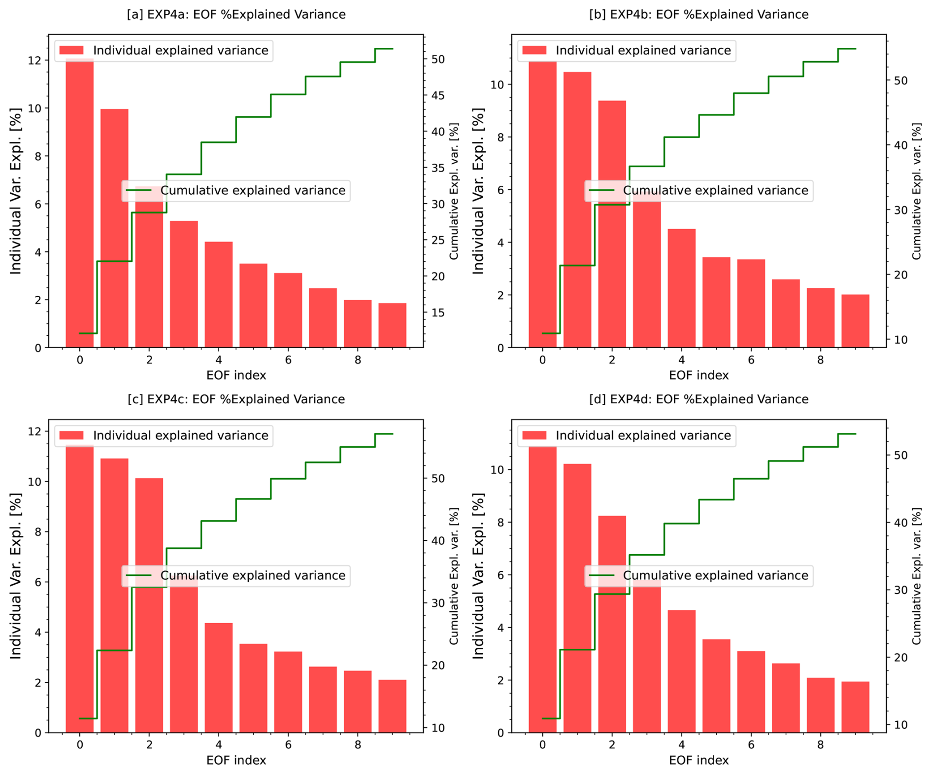
Figure A1 Contributions of variance by individual and cumulative EOFs in CLM5 soil moisture experiments. The red bars indicate the portion of variance each separate EOF mode accounts for, whereas the green line depicts the cumulative percentage of variance explained by the first 10 EOF modes. These plots show that the leading EOF modes account for a large fraction of the variance. Panels (a)–(d) correspond to EXP4a (loamy sand), EXP4b (loam), EXP4c (clay), and EXP4d (silt), respectively.

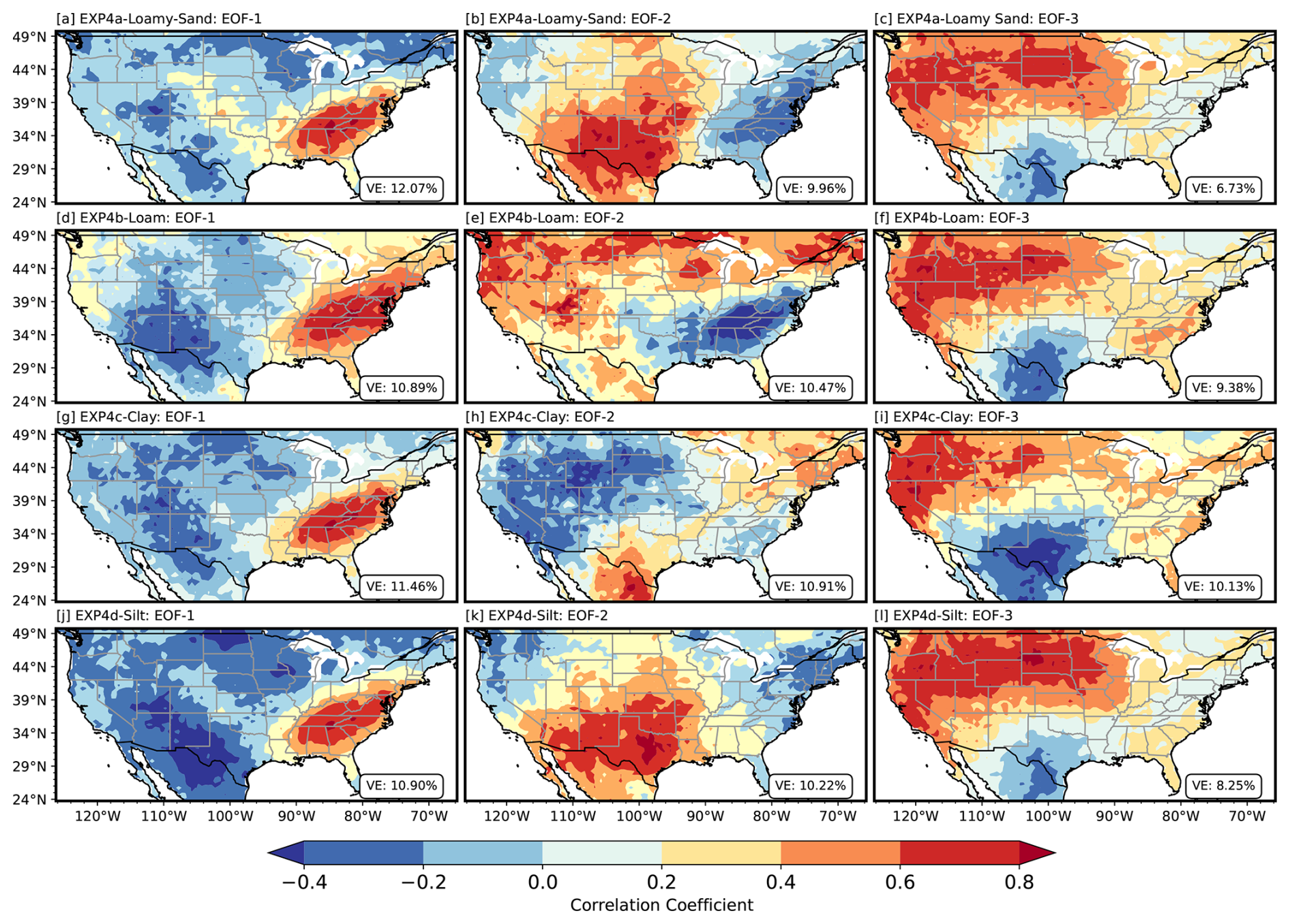
Figure A2 Spatial correlation maps of the first three empirical orthogonal functions (EOFs) of soil moisture anomalies across the CONUS domain for the EXP4 simulations. Panels (a)–(c) correspond to EXP4a (Loamy Sand), (d)–(f) to EXP4b (Loam), (g)–(i) to EXP4c (Clay), and (j)–(l) to EXP4d (Silt). Each set shows EOF-1, EOF-2, and EOF-3, respectively. The colored shading represents the correlation coefficient between the principal component (PC) time series of each EOF mode and the soil moisture anomaly time series at each grid point. Positive values (red) indicate locations that vary in phase with the mode's temporal evolution, while negative values (blue) indicate antiphase behavior. The variance explained (VE) by each mode is noted in each panel. These correlation maps illustrate how the spatial structure of soil moisture variability is influenced by distinct soil hydraulic properties associated with each texture class.

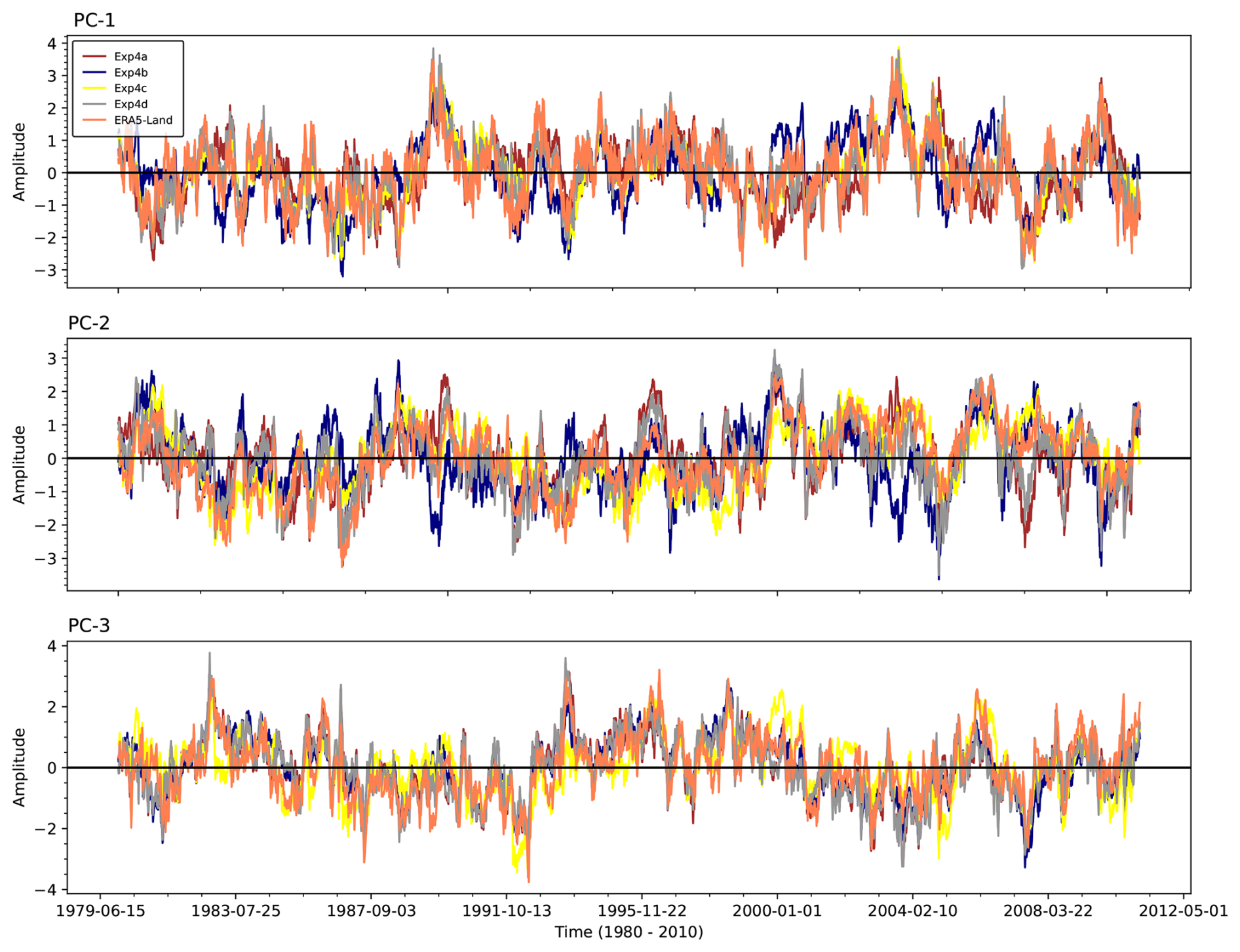
Figure A3 Temporal variability in principal components (PCs) derived from the EOF analysis. The plots display the amplitude of the first three principal components: PC-1, PC-2, and PC-3. Each line corresponds to one of the four experimental setups (EXP4a, EXP4b, EXP4c, and EXP4d) or ERA5-Land (model-based pattern reference). PC-1 (top panel) captures the dominant mode of variability, while PC-2 (middle panel) and PC-3 (bottom panel) represent the secondary and tertiary modes, respectively. The x axis shows the time period (1980–2010), and the y axis indicates the standardized amplitude. These plots highlight the temporal dynamics of soil moisture variability as captured by different experimental configurations, providing insights into their agreement and divergence relative to ERA5-Land patterns.

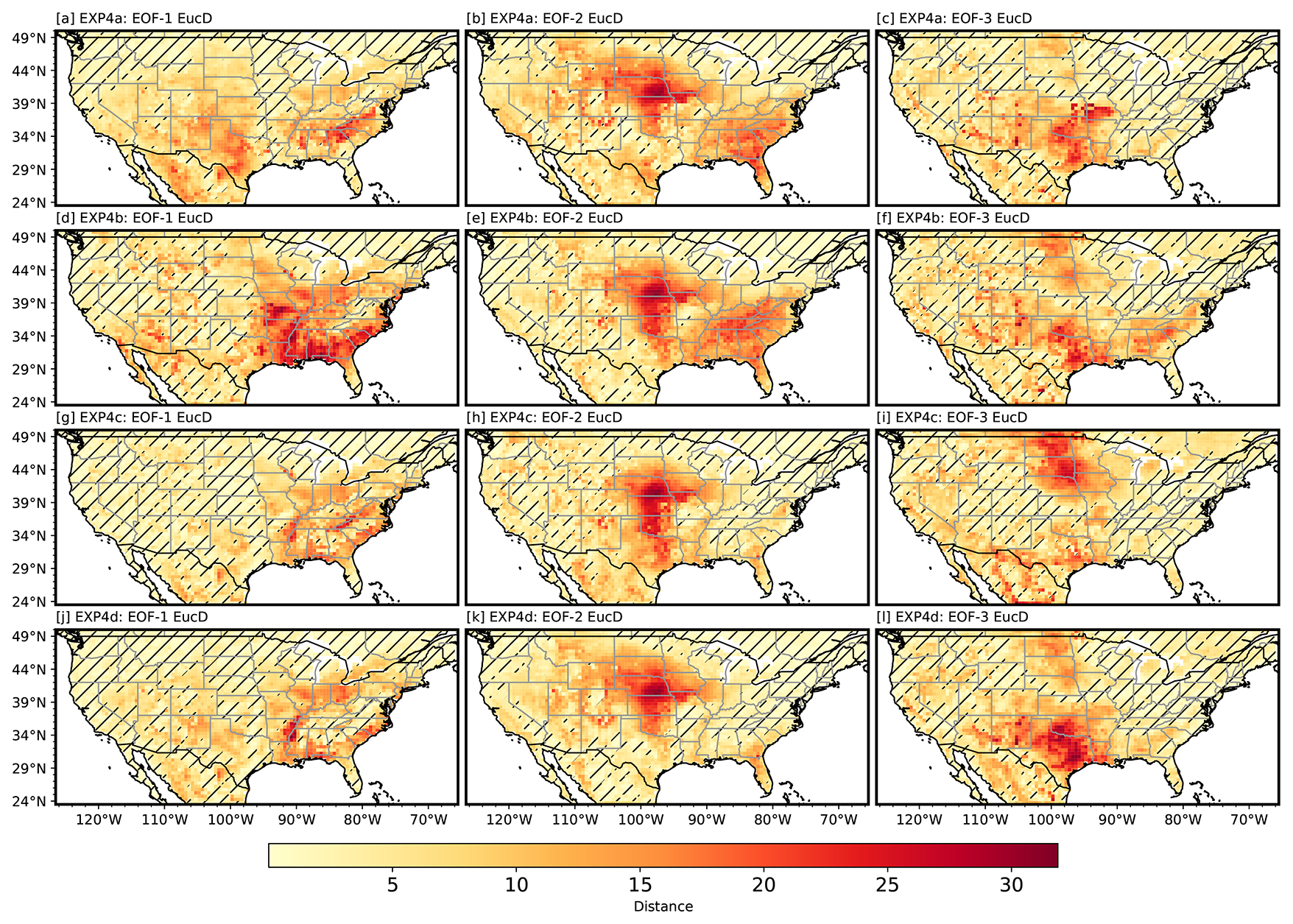
Figure A4 The Euclidean distance between EOF modes from SP-MIP experiments (EXP4a, EXP4b, EXP4c, and EXP4d) and ERA5-Land (model-based pattern reference) is shown. Panels (a)–(c) illustrate results for EXP4a (Loamy Sand), while panels (d)–(f), (g)–(i), and (j)–(l) pertain to EXP4b (Loam), EXP4c (Clay), and EXP4d (Silt), respectively. Each column showcases one of the first three EOF modes: EOF-1, EOF-2, and EOF-3. The color bar represents the Euclidean distance, where lower values (yellow) reflect greater similarity to ERA5-Land patterns, whereas higher values (red) denote more significant discrepancies. Regions with hatching signify distances of less than 5, highlighting areas with greater similarity to ERA5-Land patterns. These observations reveal the spatial variability in model similarity across different soil hydraulic parameter settings and EOF modes.