Data-Informed Inversion Model (DIIM): a framework to retrieve marine optical constituents using a three-stream irradiance model

Within the New Copernicus Capability for Trophic Ocean Networks (NECCTON) project, we aim to improve the current data assimilation system by developing a method for accurately estimating marine optical constituents from satellite-derived remote sensing reflectance. We compared two frameworks based on the implicit inversion of a semi-analytical model derived from the classical radiative transfer equation. The first approach employed an iterative Bayesian inversion with a Gaussian approximation, which provides maximum a posteriori (MAP) estimates of the optical constituents along with their associated uncertainties. To improve the model performance, we optimized the model parameters using historical in situ measurements from the BOUSSOLE buoy and a Markov chain Monte Carlo (MCMC) algorithm, which reduced the root mean square error (RMSE) between the retrieved and observed values. The second approach employed the stochastic gradient variational Bayes (SGVB) estimator, which is designed to approximate the MAP estimates of the optical constituents while simultaneously optimizing the model parameters through maximum likelihood. This method resulted in faster computations than the iterative Bayesian inversion while maintaining comparable RMSE values. While the iterative Bayesian inversion provided reliable uncertainty estimates, the SGVB estimator offered faster computations of the optical constituents. Moreover, using a dataset of in situ sea surface chlorophyll a concentrations across a broad region of the northwestern Mediterranean Sea, we compared the inversion techniques with a state-of-the-art algorithm used within the Copernicus Marine Service, finding comparable performances across methods. Notably, the SGVB estimator showed the highest correlation between in situ measurements and retrievals throughout the analyzed region. We conclude that both inversion methods achieve a performance comparable to existing state-of-the-art algorithms. The Gaussian approximation offers robust uncertainty quantification, while the SGVB estimator provides a reliable and computationally efficient alternative.

1 Introduction

Operational systems, like Copernicus, use satellite-derived data, combined with data assimilation techniques, to obtain estimates of the marine ecosystem status. Traditionally, the assimilated variable is the chlorophyll-retrieved data; nowadays, state-of-the-art biogeochemical models are progressively including refined bio-optical models able to simulate optical variables such as remote sensing reflectance, enabling the direct assimilation of multispectral reflectance measured by satellite sensors.

In this work, we aim to derive a framework to estimate ocean inherent optical properties (IOPs), such as absorption and scattering coefficients, from measurements of satellite-derived apparent optical properties (AOPs), like irradiance and remote sensing reflectance. IOPs are of interest in their own right, as they carry key information about ecosystem variables, such as chlorophyll, which can be used as indicators of the trophic condition of large marine areas (Longhurst et al., 1996). Most importantly, the framework is intended to be employed as a module in a data assimilation scheme (Bruggeman et al., 2024), within operational model services, to perform remote sensing reflectance assimilation in a coherent way, providing an aligned forward and inverse procedure.

The retrieval of the IOPs of water bodies from measurements of AOPs is referred to as the inverse problem of ocean optics. This is crucially important since directly measuring IOPs with an extended spatial coverage is very difficult (Gordon, 2002).

The first step in computing the IOPs is to establish the forward relationship between the AOPs and the IOPs. In this context, the AOPs are described as a function of the IOPs using the radiative transfer equation (RTE). Due to the complexity of the RTE, this computation is carried out in simple scenarios, resulting in simplified equations that can be solved analytically. Other approaches involve using semi-analytical equations or empirical relations, where the latter are combined with simplified expressions of the RTE. The inverse problem is solved using these forward computations to estimate the IOPs either explicitly, by analytically inverting the forward process (Zaneveld, 1989; Leathers et al., 1999; Tao et al., 1994; McCormick, 1996; Stramska et al., 2000; Salama and Verhoef, 2015; Lazzari et al., 2024), or implicitly, by using an estimate of the IOPs in the forward process and then iteratively adjusting the IOP values to match measurements of the AOPs (Gordon and Boynton, 1997; Boynton and Gordon, 2000; Michalopoulou et al., 2009; Salama and Verhoef, 2015; Erickson et al., 2023; Lazzari et al., 2024).

In this work, we focused on an implicit inverse method following Lazzari et al. (2024) but giving the method a probabilistic interpretation, allowing for the uncertainty estimation of the retrieved quantities. The forward model is the bio-optical model presented in Dutkiewicz et al. (2015) and described in Sect. 2.1, a three-stream semi-analytical irradiance model. The IOPs from the bio-optical model are the absorption, scattering, and backward-scattering coefficients of four optical constituents: water, chlorophyll α (whose increase or decrease is associated with changes in the concentration of phytoplankton), colored dissolved organic matter, and non-algal particles. We focused on finding the sea surface concentration of these optical constituents, since we estimated the former IOPs as linear combinations of the latter. The model also depends on ad hoc parameters, originally computed as part of empirical relations from different studies (Morel, 1974; Aas, 1987; Dutkiewicz et al., 2015; Mason et al., 2016; Álvarez et al., 2023). We also optimized these parameters such that the retrieved quantities are accurate with respect to historical in situ observations.

We compared two different frameworks. The first one is a Bayesian estimation, where we used a linearization of the forward process to estimate the uncertainties of the optical constituents, and Markov chain Monte Carlo (MCMC) (Chib and Greenberg, 1995; Andrieu and Thoms, 2008) to estimate the uncertainty of the parameters. This approach is described in Sect. 4.

The second approach is based on variational Bayes by using the stochastic gradient variational Bayes (SGVB) estimator, introduced by Kingma and Welling (2022) and described in Sect. 4.4. It allows for the estimation of parameters while also learning an estimate of the posterior distribution of the optical constituents. The idea is to approximate the probability distribution of the optical constituents given the satellite-derived remote sensing reflectance using a neural network. This is the same framework used to train generative models known as variational auto-encoders (VAEs), which have also been used to solve inversion problems (Zhong et al., 2020, 2021; Zhao et al., 2023; Shmakov et al., 2023). Originally proposed to solve inversion problems for cases where the posterior distribution is intractable (practically impossible to compute), this framework provides a fast way of estimating optical constituents, which are consistent with the forward model and the in situ observations.

We employed three data sources covering a period from 2005 to 2012: a dataset of historical satellite-derived remote sensing reflectance; a dataset from the Ocean–Atmosphere Spectral Irradiance Model (OASIM; used as boundary conditions for the bio-optical model; Gregg and Casey, 2009); and a set of in situ measurements from the BOUSSOLE buoy, located in the Ligurian Basin of the northwestern Mediterranean Sea (coordinates 43.22° N, 7.54° E) (Antoine et al., 2008). A description of the different datasets is presented in Sect. 3.

2 Bio-optical model

We now describe the bio-optical model (Aas, 1987; Ackleson et al., 1994; Dutkiewicz et al., 2015; Álvarez et al., 2023), which details the interaction of the radiance with different constituents in the sea, called optical constituents. In Sect. 2.1 we present the model of the water-leaving radiance, based on the classical radiative transfer model (Dutkiewicz et al., 2015). In Sect. 2.2, we use this model to compute the theoretical remote sensing reflectance ($R_{\text{rs}}^{\text{MODEL}}$) (Aas and Højerslev, 1999). The inversion problem aims to use this model, named the forward model, and satellite measurements to retrieve optical constituents that are consistent with future observations. To this end, we used historical in situ observations described in Sect. 2.3.

2.1 Radiative transfer model

To simulate the water-leaving radiance, we followed Dutkiewicz et al. (2015), using a one-dimensional, three-stream radiance model, where the vertical component of the radiance over the water column is decomposed into three interacting components (see Fig. 1) following the system of equations:

$$\begin{array}{}\text{(1)}& \begin{array}{rl}{\displaystyle \frac{\mathrm{d}{E}_{\text{dir}}(h,\mathit{\lambda })}{\mathrm{d}h}}=& -{\displaystyle \frac{a\left(\mathit{\lambda }\right)+b\left(\mathit{\lambda }\right)}{\cos \mathit{\theta }}}{E}_{\text{dir}}(h,\mathit{\lambda }),\\ {\displaystyle \frac{\mathrm{d}{E}_{\text{dif}}(h,\mathit{\lambda })}{\mathrm{d}h}}=& -{\displaystyle \frac{a\left(\mathit{\lambda }\right)+r_s{b}_b\left(\mathit{\lambda }\right)}{v_s}}{E}_{\text{dif}}(h,\mathit{\lambda })\\ & +{\displaystyle \frac{r_u{b}_b\left(\mathit{\lambda }\right)}{v_u}}{E}_{\text{u}}(h,\mathit{\lambda })\\ & +{\displaystyle \frac{b\left(\mathit{\lambda }\right)-r_d{b}_b\left(\mathit{\lambda }\right)}{\cos \mathit{\theta }}}{E}_{\text{dir}}(h,\mathit{\lambda }),\\ {\displaystyle \frac{\mathrm{d}{E}_u(h,\mathit{\lambda })}{\mathrm{d}h}}=& -{\displaystyle \frac{r_s{b}_b\left(\mathit{\lambda }\right)}{v_s}}{E}_{\text{dif}}(h,\mathit{\lambda })\\ & +{\displaystyle \frac{a\left(\mathit{\lambda }\right)+r_u{b}_b\left(\mathit{\lambda }\right)}{v_u}}{E}_u(h,\mathit{\lambda })\\ & -{\displaystyle \frac{r_d{b}_b\left(\mathit{\lambda }\right)}{\cos \mathit{\theta }}}{E}_{\text{dir}}(h,\mathit{\lambda }).\end{array}\end{array}$$

These three equations describe how the vertical direct irradiance E_dir(h,λ) is attenuated by absorption, where a(λ) is the total absorption coefficient scattered into downward E_dif(h,λ) and upward irradiance E_u(h,λ); b(λ) is the total scattering coefficient; b_b(λ) is the total backward-scattering coefficient; r_d, r_s, and r_u are the effective scattering coefficients normalized with respect to the backward-scattering coefficients cos (θ); v_s and v_u are the average cosines of the irradiance components; θ is the Sun zenith angle; h is the depth; and λ is the wavelength.

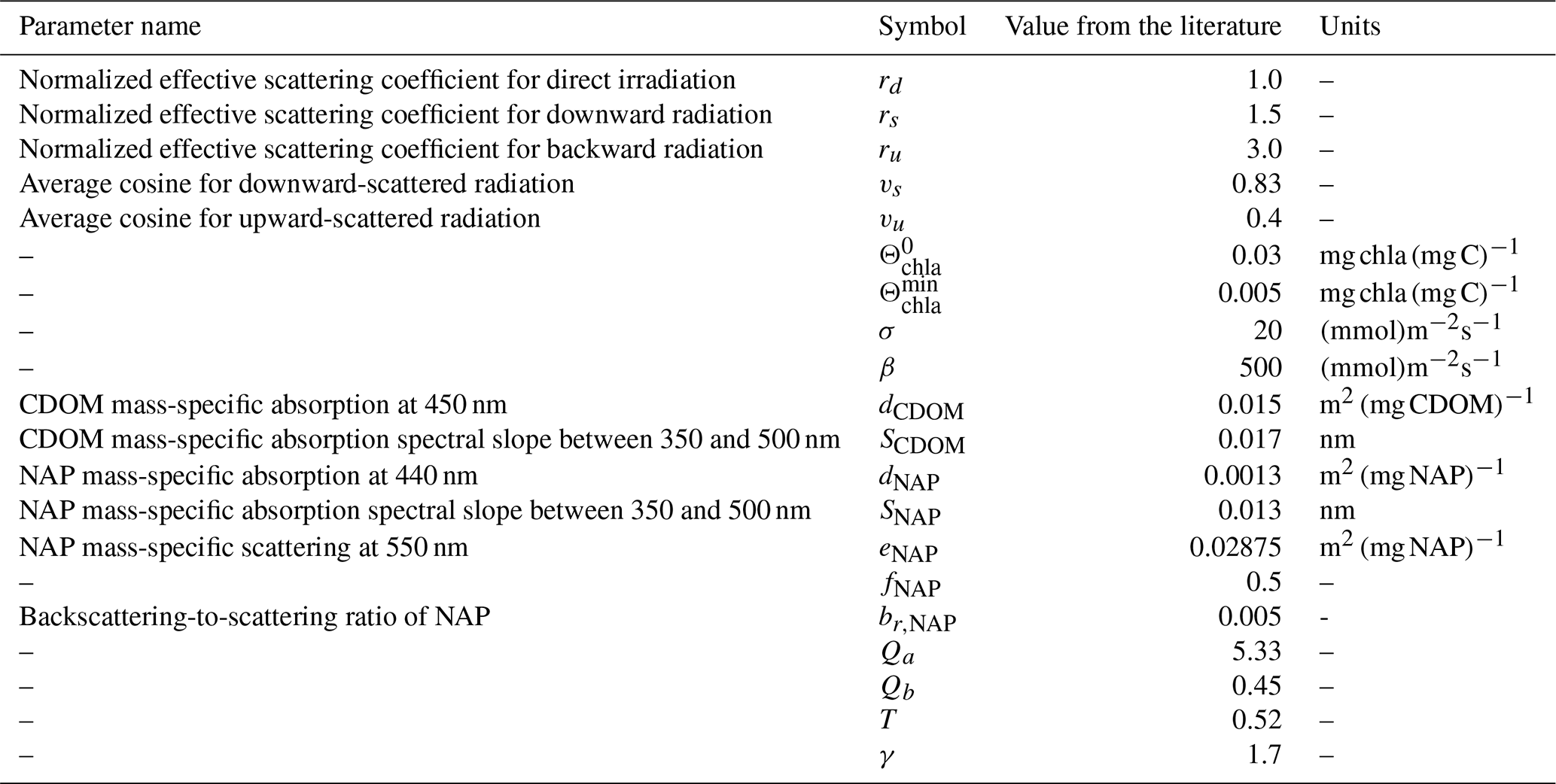
Following Dutkiewicz et al. (2015), the values for r_d, r_s, r_u, v_s, and v_u are approximated as constants (see Table 2). See Dutkiewicz et al. (2015), Appendix B, for a derivation starting from the classical radiative transfer equation. For previous studies where similar transfer models have been used, see Aas (1987), Ackleson et al. (1994), Salama and Verhoef (2015), Álvarez et al. (2023), and Lazzari et al. (2024).

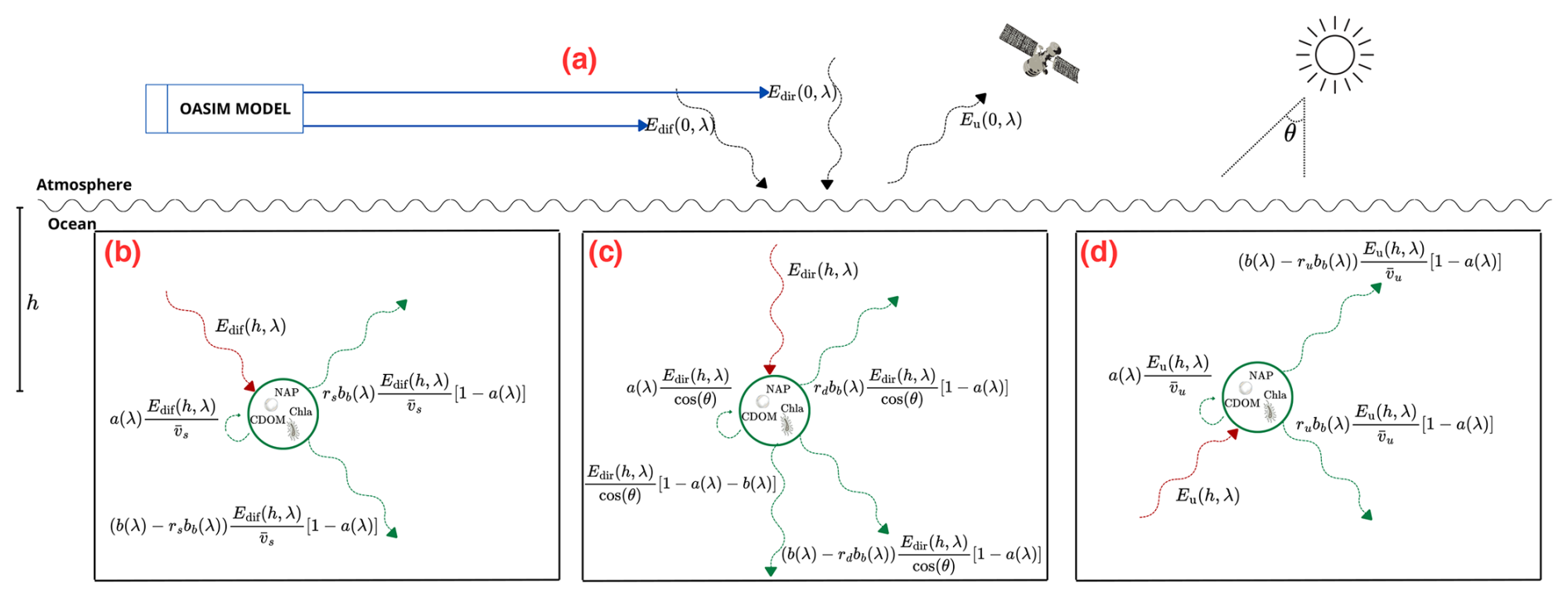
Figure 1 Diagram illustrating the main components of Eq. (1), showing (a) the incoming irradiance (modeled using OASIM; see Sect. 3) and how it interacts with chlorophyll, non-algal particles, and colored dissolved organic matter (CDOM), leading to the attenuation and scattering of (b) the diffuse, (c) direct, and (d) upward components into upward and downward fluxes.

The total absorption and scattering coefficients are modeled as

$$\begin{array}{}\text{(2)}& \begin{array}{rl}a\left(\mathit{\lambda }\right)=& a_{\text{w}}\left(\mathit{\lambda }\right)+a_{\text{phy}}\left(\mathit{\lambda }\right)\text{chla}+a_{\text{CDOM}}\left(\mathit{\lambda }\right)\text{CDOM}\\ & +a_{\text{NAP}}\left(\mathit{\lambda }\right)\text{NAP},\\ b\left(\mathit{\lambda }\right)=& b_{\text{w}}\left(\mathit{\lambda }\right)+b_{\text{phy}}\left(\mathit{\lambda }\right)C+b_{\text{NAP}}\left(\mathit{\lambda }\right)\text{NAP},\\ b_b\left(\mathit{\lambda }\right)=& b_{b,\mathrm{W}}\left(\mathit{\lambda }\right)+b_{b,\text{phy}}\left(\mathit{\lambda }\right)C+b_{b,\text{NAP}}\left(\mathit{\lambda }\right)\text{NAP},\end{array}\end{array}$$

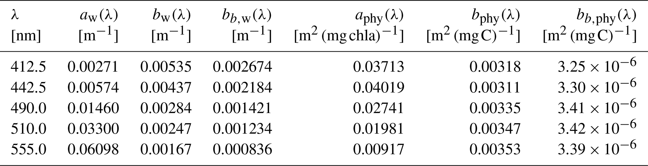
where chla, NAP, and CDOM are the concentrations of the optical constituents chlorophyll α, non-algal particles, and colored dissolved organic matter respectively; a_w(λ) is the water-specific absorption coefficient; b_w(λ) and b_b,w(λ) are the water-specific scattering and backward-scattering coefficients; a_phy(λ) is the chlorophyll-specific absorption coefficient of phytoplankton; b_phy(λ) and b_b,phy(λ) are the carbon-specific scattering coefficients of phytoplankton (see Table 1); C is the carbon concentration, which is derived as a function of chlorophyll and irradiance (Geider et al., 1997), with the chla : C ratio represented as a sigmoid curve dependent on photosynthetic available radiation (PAR) as

$$\begin{array}{}\text{(3)}& C=\text{chla}/({\mathrm{\Theta }}_{\text{chla}}^{\mathrm{0}}{\displaystyle \frac{e^{-(\text{PAR}-\mathit{\beta })/\mathit{\sigma }}}{\mathrm{1}+e^{-(\text{PAR}-\mathit{\beta })/\mathit{\sigma }}}}+{\mathrm{\Theta }}_{\text{chla}}^{\text{min}}).\end{array}$$

${\mathrm{\Theta }}_{\text{chla}}^{\mathrm{0}}$, β, σ, and ${\mathrm{\Theta }}_{\text{chla}}^{\text{min}}$ are constant parameters (see Table 2), and a_CDOM(λ), a_NAP(λ), and b_NAP(λ) are the mass-specific absorption and scattering coefficients of CDOM and NAP respectively (Álvarez et al., 2023), with the latter calculated as

$$\begin{array}{}\text{(4)}& \begin{array}{rl}& a_{\text{CDOM}}\left(\mathit{\lambda }\right)=d_{\text{CDOM}}{e}^{-S_{\text{CDOM}}(\mathit{\lambda }-\mathrm{450})},\\ & a_{\text{NAP}}\left(\mathit{\lambda }\right)=d_{\text{NAP}}{e}^{-S_{\text{NAP}}(\mathit{\lambda }-\mathrm{440})},\\ & b_{\text{NAP}}\left(\mathit{\lambda }\right)=e_{\text{NAP}}{\left({\displaystyle \frac{\mathrm{550}}{\mathit{\lambda }}}\right)}^{f_{\text{NAP}}},\end{array}\end{array}$$

where S_CDOM, d_CDOM, S_NAP, d_NAP, e_NAP, and f_NAP are constant parameters (see Table 2), and $b_{b,\text{NAP}}=b_{r,\text{NAP}}{b}_{\text{NAP}}$, with b_r,NAP being the backscattering-to-scattering ratio of NAP.

Table 1 Parameters dependent on λ used for the radiative transfer model evaluation, with the water-specific absorption coefficient a_w(λ) from Mason et al. (2016), the water-specific scattering and backward-scattering coefficients b_w(λ) and b_b,w(λ) with values interpolated from Morel (1974), the phytoplankton-specific absorption coefficient a_phy(λ) interpolated from the average values of different phytoplankton functional types from Álvarez et al. (2023), and the carbon-specific scattering and backward-scattering coefficients b_phy(λ) and b_b,phy(λ) from Dutkiewicz et al. (2015).

PAR was computed following Lazzari et al. (2021) as

$$\begin{array}{}\text{(5)}& \text{PAR}={\displaystyle \frac{{\mathrm{10}}^{\mathrm{6}}}{N_{\mathrm{A}}hc}}\underset{\mathrm{400}\mathrm{nm}}{\overset{\mathrm{700}\mathrm{nm}}{\int }}\left(E_{\text{dif}}\right(\mathrm{0},\mathit{\lambda })+E_{\text{dir}}(\mathrm{0},\mathit{\lambda }\left)\right)\mathit{\lambda }\mathrm{d}\mathit{\lambda },\end{array}$$

where N_A is Avogadro's number, c is the speed of light, and h is Planck's constant.

For the rest of this work, we assumed only one homogeneous layer with constant densities. For deep case 1 waters, like those studied in the present work, during winter, the chlorophyll concentration in the first layer is approximately constant due to mixing (see Mignot et al., 2011, Fig. 1), while most of the downward irradiance comes from the first 10 to 20 m (see Simpson and Dickey, 1981, Figs. 1 and 2). During summer, there is no mixing, but there is still a region of around 20 to 50 m with constant chlorophyll concentrations, making the assumption justified.

Table 2 Parameters independent of λ used for the radiative transfer model evaluation, r_d, r_s, r_u, v_s, v_u, S_CDOM, and d_CDOM, from Dutkiewicz et al. (2015), who took them from Aas (1987); ${\mathrm{\Theta }}_{\text{chla}}^{\text{0}}$, ${\mathrm{\Theta }}_{\text{chla}}^{\text{min}}$, σ, and β computed as an empirical model from data at the BOUSSOLE site (Lazzari et al., 2024); S_NAP, d_NAP, e_NAP, f_NAP, and b_r,NAP from Álvarez et al. (2023); Q_a and Q_b from Aas and Højerslev (1999); and T and γ from Lee et al. (2002).

2.2 Remote sensing reflectance

We used the system of equations in Eq. (1) subject to the following boundary conditions:

$$\begin{array}{}\text{(6)}& \begin{array}{rl}& E_{\text{dir}}(\mathrm{0},\mathit{\lambda })=E_{\text{dir}}^{\text{OASIM}}(\mathrm{0},\mathit{\lambda }),E_{\text{dif}}(\mathrm{0},\mathit{\lambda })=E_{\text{dif}}^{\text{OASIM}}(\mathrm{0},\mathit{\lambda }),\\ & E_{\text{u}}(\mathrm{\infty },\mathit{\lambda })=\mathrm{0},\end{array}\end{array}$$

where $E_{\text{dir}}^{\text{OASIM}}(\mathrm{0},\mathit{\lambda })$ and $E_{\text{dif}}^{\text{OASIM}}(\mathrm{0},\mathit{\lambda })$ are the direct and diffuse downward irradiance on the surface of the ocean. For this work, we used the values from OASIM (Gregg and Casey, 2009). By assuming an infinitely deep and homogeneous column of water (Ronald and Zaneveld, 1982), the system of equations can be solved analytically, with the final expression presented in Appendix A.

The remote sensing reflectance $R_{\text{rs}}^{\text{MODEL}}\left(\mathit{\lambda }\right)$ can be computed from the solution E_u(0,λ) (Aas and Højerslev, 1999) as

$$\begin{array}{}\text{(7)}& R_{\text{rs}}^{\text{MODEL}}\left(\mathit{\lambda }\right)={\displaystyle \frac{{\mathit{E}}_{u,\mathit{\lambda }}\left(\mathrm{0}\right)}{Q\left(\mathit{\theta }\right)\left({\mathit{E}}_{\text{dir},\mathit{\lambda }}\left(\mathrm{0}\right)+{\mathit{E}}_{\text{dif},\mathit{\lambda }}\left(\mathrm{0}\right)\right)}},\end{array}$$

with

$$\begin{array}{}\text{(8)}& Q\left(\mathit{\theta }\right)=Q_a{e}^{-Q_b\sin (\mathit{\pi }/\mathrm{180}(\mathrm{90}-\mathit{\theta }\left)\right)},\end{array}$$

where Q_a and Q_b are constant parameters (see Table 2).

Due to the interaction in the interface between the sea surface and the atmosphere, a correction has to be added to the $R_{\text{rs}}^{\text{MODEL}}$ (Lee et al., 2002) with the following relation:

$$\begin{array}{}\text{(9)}& {\mathit{R}}_{\text{rs,down}}\left(\mathit{\lambda }\right)={\displaystyle \frac{R_{\text{rs,up}}\left(\mathit{\lambda }\right)}{T+\mathit{\gamma }{R}_{\text{rs,up}}\left(\mathit{\lambda }\right)}},\end{array}$$

where T and γ are constant parameters (see Table 2), R_rs,down(λ) is the remote sensing reflectance just under the sea surface, and R_rs,up(λ) is the remote sensing reflectance just above the sea surface.

Thus, the final expression for $R_{\text{rs}}^{\text{MODEL}}$ is a model that depends on the optical constituents and the boundary conditions.

Since the satellite remote sensing reflectance measures are a merged product of many satellite samples (see Sect. 3) during the day, the direct and diffuse downward irradiances on the surface of the ocean were computed as daily averages only during hours with sun. For this reason, the densities involved in the computation of Eq. (7) are also daily averages.

2.3 Model of the in situ observations

We aim to model chlorophyll α as the retrieved quantity from the inversion problem. The particulate backward-scattering coefficient (b_b,p(λ)) is modeled as the contribution to backward scattering from the phytoplankton and NAP:

$$\begin{array}{}\text{(10)}& b_{b,\mathrm{p}}\left(\mathit{\lambda }\right)=b_{b,\text{phy}}\left(\mathit{\lambda }\right)C+b_{b,\text{NAP}}\left(\mathit{\lambda }\right)\text{NAP},\end{array}$$

where the carbon C is calculated as Eq. (3). The downward light attenuation coefficient (k_d) is computed by the following relation:

$$\begin{array}{}\text{(11)}& \begin{array}{rl}{E}_{\text{dir}}(h,\mathit{\lambda })& +E_{\text{dif}}(h,\mathit{\lambda })=\\ & \left(E_{\text{dir}}^{\text{OASIM}}\right(\mathrm{0},\mathit{\lambda })+E_{\text{dif}}^{\text{OASIM}}(\mathrm{0},\mathit{\lambda }\left)\right)e^{-k_{d}h}.\end{array}\end{array}$$

3 Data acquisition

3.1 Ocean–Atmosphere Spectral Irradiance Model (OASIM)

OASIM (Gregg and Casey, 2009) uses cloud, aerosol, and atmospheric conditions as input to simulate the propagation of light in the atmosphere and return the irradiance at the surface of the ocean. We used the validated outputs for the BOUSSOLE site (Antoine et al., 2008) computed in Lazzari et al. (2021) as the boundary conditions in Eq. (6). The outputs are the surface downward direct irradiance E_dir and the surface downward-scattered irradiance E_dif, from which the photosynthetic available radiation (PAR) can be computed (Lazzari et al., 2021). The output from the model is in 33 wavelengths from 200 nm to 4 µm. As described in Lazzari et al. (2021), these values are further interpolated at wavelengths 412.5, 442.5, 490, 510, and 555 nm.

3.2 Satellite-derived remote sensing reflectance

We used a Level 3 product provided by the EU Copernicus Marine Service Information (CMEMS, 2023). This is a combination of Level 2 remote sensing reflectance from different satellite sources, as explained in Colella et al. (2025). This product provides preprocessed remote sensing reflectance with daily resolution and spatial resolution of 1 km at six different wavelengths: 412, 443, 490, 510, 555, and 670 nm. Due to the fact that the absorption of water for wavelengths higher than 555 nm is dominant over the other constituents (Lee et al., 2002) for oligotrophic and mesotrophic water, we focus our attention on the data with wavelengths less than or equal to 555 nm. The values at the wavelengths 412 and 443 nm were assumed to be the same as the values with wavelengths at 412.5 and 442.5 nm in order to match the values computed with OASIM.

3.3 In situ observations

We used three in situ observations: chlorophyll α, the particulate backward-scattering coefficient, and the downward light attenuation coefficient, with data from the BOUSSOLE buoy (Antoine et al., 2008) retrieved as explained in Lazzari et al. (2024).

The three sets of measurements had a 15 min resolution. We used only measurements between 10:00 and 14:00 GMT as representative data. First, we removed the data coming from the buoy if they reported an absolute tilt higher or lower than 10°. We also removed the ones reported at a depth of more than 2 m below the nominal values (4 and 9 m, depending on the instrument of measurement). Next, the downward light attenuation coefficient data were filtered with a Butterworth high-pass filter using the SciPy package (Virtanen et al., 2020) from the Python programming language (Van Rossum and Drake, 2009), filtering the noise with a frequency of less than 4 h. Finally, we proceeded to average the daily values.

Due to low vertical variability, the measurements of chlorophyll α and the particulate backward-scattering coefficient were regarded as the values just below the water–air interface, even if the instruments were at a depth of 9 m. The former had measurements at wavelengths equal to 442, 488, 550, and 620 nm.

In contrast, due to the high vertical variability of the downward light attenuation coefficient, the measurements were considered to be at a depth of 9 m, with values at the wavelengths 412, 442, 490, 510, 555, 560, 665, 670, and 681 nm.

For the same reason described in Sect. 3.2, we only used values less than or equal to 555 nm. The values at the wavelengths 412, 442, 488, and 550 nm were assumed to be the same as the values with wavelengths at 412.5, 442.5, 490, and 555 nm in order to match the values computed with OASIM.

In other words, taking into account the previously mentioned assumptions and data availability, the in situ observations considered are sea surface chlorophyll, the 9 m deep downward light attenuation coefficient in five wavelengths (412.5, 442.5, 490, 510, 555 nm), and the sea surface particulate backward-scattering coefficient at three wavelengths (442, 490, 510 nm).

4 Bayesian inverse problem

The model for the remote sensing reflectance ($R_{\text{rs}}^{\text{MODEL}}$) depends on the concentration of the optical constituents chla, NAP, and CDOM. The inverse problem consists of retrieving these constituents from the forward model and the satellite observations ($R_{\text{rs}}^{\text{OBS}}$). In Sect. 4.1 we formalize the problem and introduce the nomenclature that is used in the next sections, and in Sect. 4.2 and 4.3 we introduce the Bayesian approach used to solve the problem (Rodgers, 2000) and the approach used to optimize the model.

4.1 Formal statement of the problem

We proceed to call y∈𝒴 the set of wavelength-dependent satellite measurements, modeled with a forward model plus noise:

$$\begin{array}{}\text{(12)}& y\left(\mathit{\lambda }\right)=R_{\text{rs}}^{\text{MODEL}}(\mathit{z},x(\mathit{\lambda }),\mathit{\lambda };\mathrm{\Lambda })+\mathit{ϵ}\left(\mathit{\lambda }\right),\end{array}$$

where

$$x\left(\mathit{\lambda }\right)=\left(E_{\text{dif}}^{\text{OASIM}}\right(\mathrm{0},\mathit{\lambda }),E_{\text{dir}}^{\text{OASIM}}(\mathrm{0},\mathit{\lambda }),\mathit{\theta },\text{PAR})$$

are the available simulated quantities, x∈𝒳, gathered from OASIM.

$$\begin{array}{rl}\mathrm{\Lambda }=(& r_s,r_u,r_d,v_s,v_u,a_{\text{w}}\left(\mathit{\lambda }\right),a_{\text{phy}}\left(\mathit{\lambda }\right),b_{\text{w}}\left(\mathit{\lambda }\right),b_{\text{phy}}\left(\mathit{\lambda }\right),\\ & b_{b,\text{W}}\left(\mathit{\lambda }\right),b_{b,\text{phy}}\left(\mathit{\lambda }\right),d_{\text{CDOM}},S_{\text{CDOM}},d_{\text{NAP}},S_{\text{NAP}},\\ & e_{\text{NAP}},f_{\text{NAP}},b_{r,\text{NAP}},{\mathrm{\Theta }}_{\text{chla}}^{\mathrm{0}},{\mathrm{\Theta }}_{\text{chla}}^{\text{min}},\mathit{\beta },\mathit{\sigma },Q_a,Q_b,T,\mathit{\gamma }),\end{array}$$

The above is the set of parameters listed together with their literature values in Tables 1 and 2, and

$$\begin{array}{}\text{(13)}& \mathit{z}=(\text{chla},\text{NAP},\text{CDOM})\end{array}$$

is the set of unknown or latent quantities z∈𝒵, which are the optical constituents.

By performing the inversion, we compute an estimate of the unknown daily quantity z^d, which only depends on the measurements and OASIM data from the same day. Each day, minimization is independent of the others, like screenshots of the state of the ocean, from which we aim to estimate the average concentrations of the active optical constituents.

Since we have measurements for a discrete set of wavelengths (at a depth h=0 m, except k_d, at a depth h=9 m), the input of the forward model is discretized as a five-dimensional vector, with each component representing values at different wavelengths. To distinguish between continuous functions and their respective discretization, λ is used as a subscript; e.g., E_dir,λ represents a component of the five-dimensional vector E_dir, with magnitudes E_dir(0,λ), where $\mathit{\lambda }=(\mathrm{412.5},\mathrm{442.5},\mathrm{490},\mathrm{510},\mathrm{555})$ nm. In a similar fashion, $x_{\mathit{\lambda }}=(E_{\text{dif},\mathit{\lambda }},E_{\text{dir},\mathit{\lambda }},\mathit{\theta },\text{PAR})$ is a component of the 4×5 tensor x. Using this notation, the measurements and OASIM data of day d are written as (y^d,x^d).

The noise ϵ is added to the model to account for the different sources of uncertainty. In this work, we assumed that ϵ is a random Gaussian variable with a mean of 0 and covariance Σ_ϵ.

As a consequence, the model of the measurement is a random variable with a Gaussian probability distribution:

$$\begin{array}{}\text{(14)}& \mathit{y}\sim p_{\mathrm{\Lambda }}\left(\mathit{y}\right|\mathit{z},\mathit{x})=\mathcal{N}({\mathit{R}}_{\text{rs}}^{\text{MODEL}}(\mathit{z},\mathit{x};\mathrm{\Lambda }),{\mathbf{\Sigma }}_{\mathit{ϵ}}).\end{array}$$

4.2 Bayesian approach to retrieve the latent variable

Under the Bayesian framework (Rodgers, 2000), the probability of the unknown quantity z, $p\left(\mathit{z}\right|\mathit{y},\mathit{x})$, given the true probability distribution of the measurement $p\left(\mathit{y}\right|\mathit{z},\mathit{x})$, can be retrieved using the Bayes theorem:

$$\begin{array}{}\text{(15)}& p\left(\mathit{z}\right|\mathit{y},\mathit{x})={\displaystyle \frac{p\left(\mathit{y}\right|\mathit{z},\mathit{x}\left)p\right(\mathit{z}\left|\mathit{x}\right)}{p\left(\mathit{y}\right|\mathit{x})}}.\end{array}$$

The probability distribution $p\left(\mathit{z}\right|\mathit{y},\mathit{x})$ is called the posterior probability distribution, or just the posterior; $p\left(\mathit{y}\right|\mathit{z},\mathit{x})$ is the likelihood; and p(z|x) is the prior probability distribution, or just the prior.

Since we are dealing with random variables, computing the posterior is equivalent to retrieving z. In the case where this computation is not possible, common approaches attempt to estimate the value of z that maximizes the posterior, named the maximum a posteriori (MAP) estimate.

In the case where little is known about the value of z, it is common practice to use an improper prior, p(z|x), as an uninformative prior, where each value of z is equally probable. With this choice of prior, the MAP is equivalent to finding the maximum likelihood estimate (MLE).

In this work, we used a log-normal distribution prior (Campbell, 1995) for the latent variable z, with parameters μ_z and Σ_z. This is equivalent to making the change of variable $\stackrel{\mathrm{̃}}{\mathit{z}}=\log \left(\mathit{z}\right)$ with a Gaussian prior with mean μ_z and covariance Σ_z. With this prior and the Gaussian likelihood, which can be derived from the forward model ${\mathit{R}}_{\text{rs}}^{\text{MODEL}}$, we can define the loss function as

$$\begin{array}{}\text{(16)}& \begin{array}{rl}{\mathcal{L}}^{z,d}({\mathit{y}}^d,& {\mathit{x}}^d,{\stackrel{\mathrm{̃}}{\mathit{z}}}^d;\mathrm{\Lambda })=-\mathrm{2}\log (p_{\mathrm{\Lambda }}\left({\stackrel{\mathrm{̃}}{\mathit{z}}}^d\right|{\mathit{y}}^d,{\mathit{x}}^d\left)\right)\\ =& ({\mathit{y}}^d-{\mathit{R}}_{\text{rs}}^{\text{MODEL}}(e^{{\stackrel{\mathrm{̃}}{z}}^d},{\mathit{x}}^d;\mathrm{\Lambda }){)}^T\\ & \times {\mathbf{\Sigma }}_{\mathit{ϵ}}^{-\mathrm{1}}({\mathit{y}}^d-{\mathit{R}}_{\text{rs}}^{\text{MODEL}}(e^{{\stackrel{\mathrm{̃}}{z}}^d},{\mathit{x}}^d;\mathrm{\Lambda }\left)\right)\\ & +({\stackrel{\mathrm{̃}}{\mathit{z}}}^d-{\mathit{\mu }}_z{)}^T{\mathbf{\Sigma }}_z^{-\mathrm{1}}({\stackrel{\mathrm{̃}}{\mathit{z}}}^d-{\mathit{\mu }}_z)+c_{\mathrm{0}},\end{array}\end{array}$$

where c₀ is a constant. It can be shown that minimizing the loss function in Eq. (16) is the same as maximizing the posterior (Rodgers, 2000). In other words, we are interested in finding the ${\stackrel{\mathrm{̃}}{\mathit{z}}}^d$ that minimizes this loss function, as an estimate of the true value for the optical constituents (under the log-normal assumptions).

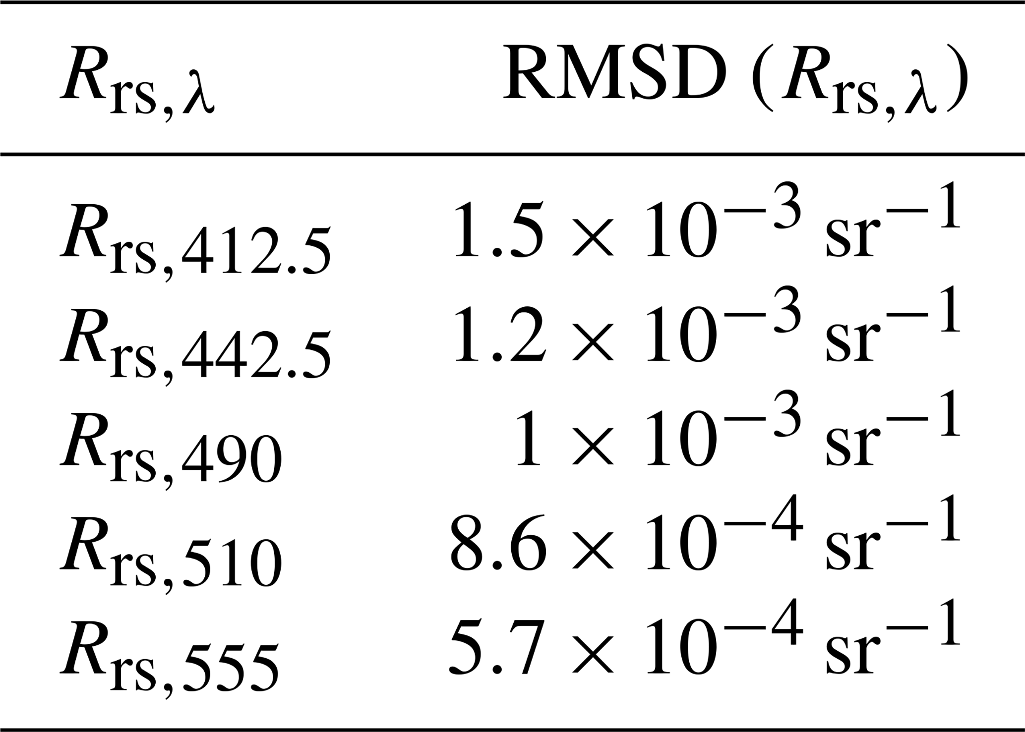
As an estimate of Σ_ϵ, we used a diagonal matrix with elements equal to the square of the root mean square difference (RMSD) between in situ measurements and the satellite measurements of R_rs in the Mediterranean Sea, shown in Table 3, obtained from a validation of the Copernicus dataset (Colella et al., 2025). This choice of Σ_ϵ is equivalent to assuming independence between measurements $y_{\mathit{\lambda }}^d$ with different wavelengths.

Table 3 Root mean square difference (RMSD) between in situ measurements and the satellite measurements of R_rs in the Mediterranean Sea, obtained from a validation of the Copernicus dataset (Colella et al., 2025).

For the prior parameters, we used μ_z=0 and Σ_z=𝟙α, with 𝟙 being a diagonal matrix of dimension 3×3 and α being a hyperparameter to be determined. This choice of Σ_z is equivalent to an ℓ₂ regularization. In Appendix B we explain the criteria used to tune α.

To retrieve ${\stackrel{\mathrm{̃}}{Z}}^{*}=\mathit{\{}{\stackrel{\mathrm{̃}}{\mathit{z}}}^{d*}{\mathit{\}}}_{d=\mathrm{1}}^D$, the MAP estimate of the latent variable $\stackrel{\mathrm{̃}}{\mathit{z}}$ for each day d, we want to minimize ℒ^z,d with respect to ${\stackrel{\mathrm{̃}}{\mathit{z}}}^d$ for every day d. We can perform this retrieval for all the historical data by minimizing the loss function; i.e., we aim to find

$$\begin{array}{}\text{(17)}& \begin{array}{rl}{\stackrel{\mathrm{̃}}{Z}}^{*}& ={\text{argmin}}_{\stackrel{\mathrm{̃}}{Z}}{\mathcal{L}}^z\\ & ={\text{argmin}}_{\stackrel{\mathrm{̃}}{Z}}\sum _{d=\mathrm{0}}^D{\mathcal{L}}^{z,d}({\mathit{y}}^d,{\mathit{x}}^d,{\stackrel{\mathrm{̃}}{\mathit{z}}}^d;\mathrm{\Lambda }).\end{array}\end{array}$$

4.2.1 Estimation of the latent variable posterior

We performed the minimization of ℒ^z using the Adam algorithm, with a learning rate γ=0.03, β₁=0.9, and β₂=0.999, which are the default momentum parameters from the PyTorch library (Paszke et al., 2019) version 2.4.1. We used 90 % of all the historical data per iteration, selected randomly across the entire period. The remaining 10 % were used as the test set. A copy of the code availability for every algorithm described in this work is in Soto (2025).

After ${\stackrel{\mathrm{̃}}{Z}}^{*}$ (the set of latent variables for the entire training set) was retrieved in order to estimate the uncertainty, we linearized ${\mathit{R}}_{\text{rs}}^{\text{MODEL}}(e^{{\stackrel{\mathrm{̃}}{z}}^d},\mathit{x};\mathrm{\Lambda })$ around ${\stackrel{\mathrm{̃}}{\mathit{z}}}^{d*}$ as

$$\begin{array}{}\text{(18)}& \begin{array}{rl}{\mathit{R}}_{\text{rs}}^{\text{MODEL}}& (e^{{\stackrel{\mathrm{̃}}{z}}^d},\mathit{x};\mathrm{\Lambda })\\ \approx & {\mathit{R}}_{\text{rs}}^{\text{MODEL}}(e^{{\stackrel{\mathrm{̃}}{z}}^{d*}},\mathit{x};\mathrm{\Lambda })\\ & +{\mathrm{\nabla }}_{{\stackrel{\mathrm{̃}}{z}}^d}{\mathit{R}}_{\text{rs}}^{\text{MODEL}}(e^{{\stackrel{\mathrm{̃}}{z}}^d},\mathit{x};\mathrm{\Lambda }){|}_{({\stackrel{\mathrm{̃}}{z}}^d={\stackrel{\mathrm{̃}}{z}}^{d*})}({\stackrel{\mathrm{̃}}{\mathit{z}}}^d-{\stackrel{\mathrm{̃}}{\mathit{z}}}^{d*})\\ =& {\mathit{R}}_{\text{rs}}^{\text{MODEL}}(e^{{\stackrel{\mathrm{̃}}{z}}^{d*}},\mathit{x};\mathrm{\Lambda })+\mathbf{K}({\stackrel{\mathrm{̃}}{\mathit{z}}}^d-{\stackrel{\mathrm{̃}}{\mathit{z}}}^{d*}),\end{array}\end{array}$$

where K is the Jacobian of ${\mathit{R}}_{\text{rs}}^{\text{MODEL}}(e^{{\stackrel{\mathrm{̃}}{z}}^{d*}},\mathit{x};\mathrm{\Lambda })$ with respect to ${\stackrel{\mathrm{̃}}{\mathit{z}}}^d$. Then, as shown in Rodgers (2000), the covariance matrix of the approximate posterior can be written as

$$\begin{array}{}\text{(19)}& {\mathbf{\Sigma }}_{{\stackrel{\mathrm{̃}}{z}}^{d*}}=({\mathbf{K}}^T{\mathbf{\Sigma }}_{\mathit{ϵ}}^{-\mathrm{1}}\mathbf{K}+{\mathbf{\Sigma }}_z^{-\mathrm{1}}{)}^{-\mathrm{1}}.\end{array}$$

In this way, the standard deviation is computed as the root square of the diagonal elements ${\mathit{\sigma }}_{\stackrel{\mathrm{̃}}{z}}$ of ${\mathbf{\Sigma }}_{{\stackrel{\mathrm{̃}}{z}}^{d*}}$.

Then, since the resulting retrieved values ${\stackrel{\mathrm{̃}}{Z}}^{*}$ are normally distributed, $Z^{*}=\text{exp}\left({\stackrel{\mathrm{̃}}{Z}}^{*}\right)$ has a log-normal distribution, and the uncertainty can thus be computed with the 68 % confidence interval (here we match the convention of using the standard deviation as uncertainty for variables with normal distribution).

The uncertainty for derived variables like kd and b_b,p is computed with standard error propagation (Arras, 1998); i.e., ΔF(x)²=∇_xF(x)Σ^x∇_xF(x)^T, where ΔF(x) is the error of a function F(x), ∇_xF(x) is the Jacobian, and Σ^x is the covariance matrix of x (in our case, ${\mathbf{\Sigma }}^x={\mathbf{\Sigma }}_{{\stackrel{\mathrm{̃}}{z}}^{d*}}$). These equations assume that each component of x is not correlated with the others and is only an approximation for nonlinear functions.

The previous procedure is equivalent to estimating the latent variable posterior with a log-normal distribution. A comparison of the true posterior and the estimated posterior can be seen in Fig. 7, where the true posterior was computed by sampling using the Metropolis–Hasting algorithm (see Algorithm 2). The discrepancy between the mean and standard deviation is due to the linearization step in Eq. (18). Algorithm 1 summarizes the steps used for the posterior estimate.

Algorithm 1 Algorithm for estimating the daily posterior estimate of the unknown latent variable z^d and the derived quantities kd^d and ${{\mathit{b}}_{\text{bp}}}^d$:
Input: x^d, y^d.

1. Find ${\stackrel{\mathrm{̃}}{\mathit{z}}}^{d*}={\text{argmin}}_{{\stackrel{\mathrm{̃}}{z}}^d}{\mathcal{L}}^{z,d}({\mathit{y}}^d,{\mathit{x}}^d,{\stackrel{\mathrm{̃}}{\mathit{z}}}^d;\mathrm{\Lambda })$ using a minimization algorithm (for example, Adam).

2. Compute K, the Jacobian of ${\mathit{R}}_{\text{rs}}^{\text{MODEL}}(e^{{\stackrel{\mathrm{̃}}{z}}^{d*}},\mathit{x};\mathrm{\Lambda })$, with respect to ${\stackrel{\mathrm{̃}}{\mathit{z}}}^d$.

3. Compute the covariance matrix of the approximate posterior as ${\mathrm{\Sigma }}_{{\stackrel{\mathrm{̃}}{z}}^{d*}}=({\mathbf{K}}^T{\mathbf{\Sigma }}_{\mathit{ϵ}}^{-\mathrm{1}}\mathbf{K}+{\mathbf{\Sigma }}_z^{-\mathrm{1}}{)}^{-\mathrm{1}}$.

4. The MAP estimate of the latent variable is equal to ${\mathit{z}}^{d*}=e^{{\stackrel{\mathrm{̃}}{z}}^{d*}}$. The uncertainty can be found by computing the 68 % confidence interval of the log-normal distribution. For this work, only the diagonal elements of ${\mathbf{\Sigma }}_{{\stackrel{\mathrm{̃}}{z}}^{d*}}$ were used, assuming independence between the latent variables.

5. Use Eqs. (10) and (11) to compute ${\mathit{b}}_{\text{bp}}^d$ and kd^d respectively, and use standard error propagation for their uncertainties.

4.3 Model optimization scheme

We retrieved the latent variable posterior in order to accurately estimate the daily average of chlorophyll, non-algal particles, and colored dissolved organic matter concentrations. To assess the accuracy of the inversion, we used the in situ observations $H^{\text{OBS}}=\mathit{\left\{}\right(\mathit{k}{\mathit{d}}^{d,\text{obs}},{{\mathit{b}}_{\text{bp}}}^{d,\text{obs}},{\text{chla}}^{d,\text{obs}}){\mathit{\}}}_{d=\mathrm{1}}^D$, where D is the number of days with available observations, kd^d,obs is a five-dimensional vector containing daily in situ observations of the downward light attenuation coefficient, ${{\mathit{b}}_{\text{bp}}}^{d,\text{obs}}$ is a three-dimensional vector with observations of the particulate backward-scattering coefficient only for the wavelengths $\mathit{\lambda }=(\mathrm{442.5},\mathrm{490},\mathrm{555}\mathrm{nm}$), and chla^d,obs is a scalar observation of sea surface chlorophyll concentration.

By comparing the modeled observation operator $H^{\text{MODEL}}=\left(\mathit{k}\mathit{d}\right({\mathit{z}}^d;{\mathit{x}}^d,\mathrm{\Lambda }),{\mathit{b}}_{\text{bp}}({\mathit{z}}^d;{\mathit{x}}^d,\mathrm{\Lambda }),\text{chla})$ with the daily observations, we aimed to optimize the forward model ${\mathit{R}}_{\text{rs}}^{\text{MODEL}}(\stackrel{\mathrm{̃}}{\mathit{z}},{\mathit{x}}^d;\mathrm{\Lambda })$ by adjusting the parameters Λ. We looked for Λ^* such that ${\sum }_{d=\mathrm{1}}^D\left|\right|H^{\text{MODEL}}({\mathit{z}}^{d*};{\mathit{x}}^d,{\mathrm{\Lambda }}^{*})-H^{\text{OBS}}\left|\right|$ is minimized for some suitable choice of distance. Since observations are not available every day and the observations corresponding to some of the wavelengths are missing, we worked with daily vectors with a dimension equal to the total number of available observations; e.g., days with all observations available correspond to vectors of dimension nine (five for kd^d, three for b_bp, and one for chla), while days with fewer observations correspond to lower-dimensional vectors.

Since we also want to estimate the uncertainty of the retrieved parameters, we used the standard deviation over all the training data as a measure of the spread of each observation and defined the loss function as

$$\begin{array}{}\text{(20)}& {\mathcal{L}}^H=\sum _{d=\mathrm{0}}^D{\displaystyle \frac{{\left({\text{H}}^{\text{MODEL},d}(Z^{*};\mathit{X},\mathrm{\Lambda })-H^{\text{OBS},d}\right)}^{\mathrm{2}}}{{\mathit{\sigma }}_{\text{OBS}}^{\mathrm{2}}}},\end{array}$$

where σ_OBS is the standard deviation of the observations computed only with the training data. We want to minimize this loss function and obtain an estimate for the uncertainty of the retrieved parameters. For this purpose, we proceed to use a Markov chain Monte Carlo algorithm, described in the next section.

4.3.1 Markov chain Monte Carlo algorithm for optimizing the model parameters

In order to estimate the posterior distribution of the parameters, $p\left(\mathrm{\Lambda }\right|H^{\text{OBS}},\widehat{Z},\mathit{X})$, we used the Metropolis–Hasting algorithm (Chib and Greenberg, 1995; Andrieu and Thoms, 2008).

The algorithm returns samples from a probability density function π(x) by defining a Markov process with a transition probability p(x,y) of moving from state x to state y. It can be shown that, with a suitable definition of this transition probability, the Markov chain process can converge asymptotically to the target distribution π(x). The Metropolis–Hasting algorithm uses the following transition probability:

$$\begin{array}{}\text{(21)}& \begin{array}{rl}p(x,y)& =q(x,y)\mathit{\alpha }(x,y),\\ \mathit{\alpha }(x,y)& =\text{min}\left[{\displaystyle \frac{\mathit{\pi }\left(y\right)q(y,x)}{\mathit{\pi }\left(x\right)q(x,y)}},\mathrm{1}\right],\end{array}\end{array}$$

where q(x,y) is the proposal transition probability, and α(x,y) is the acceptance probability. With this definition, samples from π(x) can be drawn by following Algorithm 2.

Algorithm 2 Metropolis–Hasting algorithm (Chib and Greenberg, 1995; Andrieu and Thoms, 2008). It consists of defining a Markov process. It is useful to sample from a target distribution π(x) without knowing the normalization constant.
Define: Proposal transition probability q(x,y).
Input: Length L_chain.
Initialize: x₀.

1. a = array of length L_chain.

2. a[0] = x₀.

3. For i = 0 to i = L_m−1 do

1. Sample a proposed new point $y\sim q\left(a\right[i],y$).

2. Compute α(a[i],y) as stated in Eq. (21).

3. Sample a random number from a uniform distribution between 0 and 1.

If the output is smaller than $\mathit{\alpha }\left(a\right[i],y)a[i+\mathrm{1}]=y$ else $a[i+\mathrm{1}]=a\left[i\right]$.

4. Discard the first samples (reaching the asymptotical behavior) and the correlated ones.

Some drawbacks are known; for example, the iterations have to be performed multiple times before the algorithm converges to its asymptotical behavior or successive iterations tend to be strongly correlated, so many iterations have to be performed in order to obtain uncorrelated samples. These difficulties increase as the dimensionality of the sampling space gets higher. In our case, to mitigate some of these effects, we did not perturb all the parameters, leaving those that are more precisely measured in the literature unperturbed, like the water-specific absorption and scattering coefficients.

A further complication is that the probability density that we want to sample depends on Z^*, the latent variable. This means that, each time we want to perform an iteration of the Metropolis–Hasting algorithm, we would need to find the MAP estimate of Z, increasing the computational time. To mitigate this problem, we use an estimate $\widehat{Z}$, consisting of a few iterations towards the MAP estimate.

Our model for the negative log likelihood is the loss function ℒ^H described in Sect. 4.3, which gives us the expression for the likelihood:

$$\begin{array}{}\text{(22)}& p\left(H^{\text{OBS}}\right|\mathrm{\Lambda },\widehat{Z},\mathit{X})\propto e^{-\frac{\mathrm{1}}{\mathrm{2}}{\mathcal{L}}^H(H^{\text{OBS}},\widehat{Z},\mathit{X},\mathrm{\Lambda })}.\end{array}$$

The density function, π(x), that we want to sample from is the posterior probability for the parameters. By using a uniform prior, $q({\mathrm{\Lambda }}_i,{\mathrm{\Lambda }}_j)=\mathcal{N}({\mathrm{\Lambda }}_i,{\mathit{\alpha }}_q\mathbb{1})$, where α_q is a hyperparameter equal to the standard deviation of the distance between steps. We compute the acceptance probability as

$$\begin{array}{}\text{(23)}& \begin{array}{rl}\mathit{\alpha }& ({\mathrm{\Lambda }}_i,{\mathrm{\Lambda }}_j)=\\ & \text{min}\left[e^{-\frac{\mathrm{1}}{\mathrm{2}}\left({\mathcal{L}}^H\right(H^{\text{OBS}},\widehat{Z},\mathit{X},{\mathrm{\Lambda }}_j)-{\mathcal{L}}^H(H^{\text{OBS}},\widehat{Z},\mathit{X},{\mathrm{\Lambda }}_i\left)\right)},\mathrm{1}\right].\end{array}\end{array}$$

Regarding the perturbed parameters, we consider the literature values Λ⁰ as close estimates of the optimal ones. For this reason, we perturbed them as ${\mathrm{\Lambda }}^{*}={\mathit{\delta }}_{\mathrm{\Lambda }}^T{\mathrm{\Lambda }}^{\mathrm{0}}$, where δ_Λ is a vector of small perturbations from unity, referred to as perturbation factors.

The values of the λ-dependent vector of dimension five, representing the phytoplankton-specific absorption coefficients a_phy, were perturbed as ${\mathit{a}}_{\text{phy}}^{*}={\mathit{\delta }}_{a_{\text{phy}}}{\mathit{a}}_{\text{phy}}^{\mathrm{0}}$, with ${\mathit{\delta }}_{a_{\text{phy}}}$ being a learnable scalar and ${\mathit{a}}_{\text{phy}}^{\mathrm{0}}$ the literature values. This formulation was chosen to maintain the shape of the function a_phy(λ) unperturbed.

For the carbon-specific scattering and backscattering coefficients b_phy(λ) and b_b,phy(λ), we first linearly interpolated them with the literature values and perturbed the tangent and the intercept of the linear interpolations, $b_{\text{phy}}(\mathit{\lambda }{)}^{*}={\mathit{\delta }}_{b_{\text{phy,int}}}{b}_{\text{phy,int}}^{\mathrm{0}}+{\mathit{\delta }}_{b_{\text{phy,T}}}{b}_{\text{phy,T}}^{\mathrm{0}}\mathit{\lambda }$.

The perturbations of the parameters d_CDOM, b_r,NAP, S_CDOM, ${\mathrm{\Theta }}_{\text{chla}}^{\text{min}}$, ${\mathrm{\Theta }}_{\text{chla}}^{\text{0}}$, β, σ, Q_a, and Q_b consisted of per-parameter scalar multiplications. All the other parameters were left unperturbed.

In this way, we perturbed 24 parameters, 9 of them by multiplying them by a scalar δ_i, where i is equal to each of the perturbed parameters; the 5 components of a_phy by multiplying them by the same scalar ${\mathit{\delta }}_{a_{\text{phy}}}$; and, finally, b_phy(λ) and b_b,phy(λ) by linearly interpolating them and perturbing the tangent and the intercept of each of them, totaling 14 perturbation factors.

In this manner, the perturbations δ_Λ were initialized with ones, and alternate minimization (AM) was then used, alternating between finding the MAP estimate of Z^* and the MLE of the parameters. Finally, we used the Metropolis–Hasting algorithm to estimate the posterior, as described in Algorithm 3.

Algorithm 3 Metropolis–Hasting algorithm with alternate minimization. Here we expand the Metropolis–Hasting algorithm in combination with the alternate minimization to sample from the posterior probability of the parameter space.
Define: Transition probability $q({\mathrm{\Lambda }}_i,{\mathrm{\Lambda }}_j)=\mathcal{N}({\mathrm{\Lambda }}_i,{\mathit{\alpha }}_q\mathbb{1})$.
Input: L_chain (length of MCMC chains), N_steps (number of AM steps), N_{z_steps} (steps towards the min of z^*).
Initialize: Λ₀ as the literature values.

1. Alternate minimization to estimate the MLE of the parameters.

1. For i=0 to i=N_steps

– Find an estimate of all the latent variables ${\widehat{Z}}^{*}\approx {\text{argmin}}_{\stackrel{\mathrm{̃}}{z}}{\mathcal{L}}^z(\mathit{y},\mathit{x},\stackrel{\mathrm{̃}}{\mathit{z}};{\mathrm{\Lambda }}_{\mathrm{0}})$

by performing N_{z_steps} iterations towards the minimum of the loss function.

– Perform one step towards the minimization of ${\mathcal{L}}^{\text{H}}(\mathit{y},\mathit{x},{\widehat{Z}}^{*};{\mathrm{\Lambda }}_{\mathrm{0}})$ and set Λ₀ to the new value.

2. Define an empty array Λ of length L_chain.

3. Λ[0] = Λ₀.

4. For i=0 to $i=L_{\text{chain}}-\mathrm{1}$

1. Sample a proposed new point ${\mathrm{\Lambda }}_j\sim \mathcal{N}\left(\mathrm{\Lambda }\right[i],{\mathit{\alpha }}_q\mathbb{1})$.

2. Find an estimate of all the latent variables ${\widehat{Z}}^{*}\approx {\text{argmin}}_{\stackrel{\mathrm{̃}}{z}}{\mathcal{L}}^z(\mathit{y},\mathit{x},\stackrel{\mathrm{̃}}{z};{\mathrm{\Lambda }}_j)$ by performing

a finite number of iterations towards the minimum of the loss function.

2. Compute α(Λ_i,Λ_j) as stated in Eq. (23) using the estimate ${\widehat{Z}}^{*}$ instead of the true minimum Z^*.

3. Sample a random number from a uniform distribution between 0 and 1. If the output is smaller

than α(Λ_i,Λ_j), make Λ[i+1] = Λ_j else Λ[i+1] = Λ[i].

5. Discard the first samples (reaching the asymptotical behavior) and the correlated ones.

4.4 Data-Informed Inversion Method (DIIM): a variational Bayes approach

As the dimension of the posterior increases, MCMC methods become increasingly more challenging, and even pointwise estimates, like those obtained with alternate minimization, could not converge due to the nonconvexity of our models. As an alternative approach, we present a framework based on the stochastic gradient variational Bayes (SGVB) estimator (Kingma and Welling, 2022).

The SGVB-based framework considers a random latent variable z∈𝒵 sampled from an unknown distribution $p_{{\mathrm{\Lambda }}^{*}}\left(\mathit{z}\right)$ and a random variable y∈𝒴 sampled from a distribution $p_{{\mathrm{\Lambda }}^{*}}\left(\mathit{y}\right|\mathit{z})$ conditional on the latent variable z. For example, y could be measurements from a known physical process, conditional on unknown hidden physical processes.

The aim is to efficiently approximate the maximum marginal likelihood estimate of the parameters Λ:

$$\begin{array}{}\text{(24)}& {\mathrm{\Lambda }}^{*}={\text{argmax}}_{\mathrm{\Lambda }}\left(p_{\mathrm{\Lambda }}\right(\mathit{y}\left)\right).\end{array}$$

To this end, the posterior probability distribution p_Λ(z|y) is estimated as a parameterized function q_ϕ(z|y). It can be shown that finding Λ^* and ϕ^* such that

$$\begin{array}{}\text{(25)}& \begin{array}{rl}{\mathrm{\Lambda }}^{*},{\mathit{\varphi }}^{*}=& {\text{argmax}}_{\mathrm{\Lambda },\mathit{\varphi }}{\mathcal{L}}_{\text{ELBO}},\\ {\mathcal{L}}_{\text{ELBO}}=& -D_{\text{KL}}\left(q_{\mathit{\varphi }}\right(\mathit{z}\left|\mathit{y}\right)\left|\right|p_{\mathrm{\Lambda }}\left(\mathit{z}\right))\\ & +{\mathbb{E}}_{q_{\mathit{\varphi }}\left(z\right|\mathit{y})}\left[\log \right(p_{\mathrm{\Lambda }}\left(\mathit{y}\right|\mathit{z}\left)\right)]\end{array}\end{array}$$

is approximately equal to finding the maximum likelihood estimate. Here $D_{\text{KL}}(\cdot ||\cdot )$ is the Kullback–Leibler divergence (D_KL), an asymmetric, positively defined measure of the proximity between two probability distributions (Shlens, 2014); p_Λ(z) is the prior distribution of the latent variable z; and ${\mathbb{E}}_{q_{\mathit{\varphi }}\left(\mathit{z}\right|\mathit{y})}[\cdot ]$ stands for the expected value over the probability distribution q_ϕ(z|y).

This is because ℒ_ELBO, where ELBO stands for “evidence lower bound”, is a lower bound of the data log-likelihood log p_Λ(y) (see Appendix C).

Kingma and Welling (2022) presented the SGVB estimator for the expected value (in the case where the D_KL can not be computed analytically, it can also be estimated) as

$$\begin{array}{}\text{(26)}& \begin{array}{rl}{\widehat{\mathcal{L}}}_{\text{ELBO}}\approx & -D_{\text{KL}}\left(q_{\mathit{\varphi }}\right(\mathit{z}\left|\mathit{y}\right)\left|\right|p_{\mathrm{\Lambda }}\left(\mathit{z}\right))\\ & +{\displaystyle \frac{\mathrm{1}}{L}}\sum _{l=\mathrm{1}}^L\log \left(p_{\mathrm{\Lambda }}\right(\mathit{y}\left|{\mathit{z}}_l\right)),z_l\sim q_{\mathit{\varphi }}(\mathit{z}|\mathit{y},\mathit{x}).\end{array}\end{array}$$

If the SGVB is used with a neural network as the approximate probability distributions q_ϕ(z|y), then the neural network architecture and minimization scheme are known as variational auto-encoders (Kingma and Welling, 2022), where the model q_ϕ(z|y) is usually called the “encoder” and p_Λ(y|z) the “decoder”.

Sohn et al. (2015) generalized this framework for what they called conditional variational auto-encoders (CVAEs), where the likelihood and posterior probabilities are allowed to be conditional distributions on a third set of random variables x∈𝒳, $\mathit{y}\sim p_{\mathrm{\Lambda }}\left(\mathit{y}\right|\mathit{z},\mathit{x})$ and $\mathit{z}\sim q_{\mathit{\varphi }}\left(\mathit{z}\right|\mathit{y},\mathit{x})$. This is the final configuration we used, but instead of training a generative model, as CVAEs are usually used to, we used it to solve the inversion problem while simultaneously finding approximate values for the parameters Λ^*, as explained in Sect. 4.4.1.

4.4.1 Variational Bayes approach to solve the inversion problem with the SGVB estimator

CVAEs are commonly used to train a generative model $p_{\mathrm{\Lambda }}\left(\mathit{y}\right|\mathit{z},\mathit{x})$ from a probability distribution p(z|x) that is easy to sample, in order to generate samples that effectively approximate the target probability distribution (Doersch, 2021). They have been used to solve inverse problems, like image recovery (Zhong et al., 2020, 2021; Zhao et al., 2023) and unfolding in high-energy physics (Shmakov et al., 2023), among other applications. In contrast to previous applications of VAEs and CVAEs to inverse methods, in this work, instead of first training a CVAE with latent variables that lack a physical interpretation, we directly used the SGVB estimator for the inverse method. Here, $p_{\mathrm{\Lambda }}\left(\mathit{y}\right|\mathit{z},\mathit{x})$ is the likelihood described in Eq. (14), where Λ represents the parameters of the forward function that we aim to optimize, and the latent variable z is the vector that we want to retrieve.

To do so, we used a neural network $q_{\mathit{\varphi }}\left(\mathit{z}\right|\mathit{y},\mathit{x})$ (diagram shown in Fig. 3) as an approximation of the posterior $p\left(\mathit{z}\right|\mathit{y},\mathit{x})$.

Our model for the likelihood is

$$\begin{array}{}\text{(27)}& \begin{array}{rl}-{\displaystyle \frac{\mathrm{1}}{L}}\sum _{l=\mathrm{1}}^L& \log \left(p_{\mathrm{\Lambda }}\right(\mathit{y}\left|{\mathit{z}}_l\right))=\\ {\displaystyle \frac{\mathrm{1}}{\mathrm{2}L}}& \sum _{l=\mathrm{0}}^L({\mathit{y}}^d-{\mathit{R}}_{\text{rs}}^{\text{MODEL}}(e^{{\stackrel{\mathrm{̃}}{z}}^d},{\mathit{x}}^d;\mathrm{\Lambda }){)}^T\\ & \times {\mathbf{\Sigma }}_{\mathit{ϵ}}^{-\mathrm{1}}({\mathit{y}}^d-{\mathit{R}}_{\text{rs}}^{\text{MODEL}}(e^{{\stackrel{\mathrm{̃}}{z}}^d},{\mathit{x}}^d;\mathrm{\Lambda }\left)\right)\\ +& \left({\mathcal{H}}^d\right(e^{{\stackrel{\mathrm{̃}}{z}}^d},\mathit{X};\mathrm{\Lambda })-H^{\text{OBS},d}{)}^T\\ & \times {\mathbf{\Sigma }}_H^{-\mathrm{1}}\left({\widehat{\mathcal{H}}}^d\right(e^{{\stackrel{\mathrm{̃}}{z}}^d},\mathit{X};\mathrm{\Lambda })-H^{\text{OBS},d}),\end{array}\end{array}$$

where ${\mathbf{\Sigma }}_{\mathit{ϵ}}^{-\mathrm{1}}$ is the equivalent to the covariance matrix introduced in Sect. 4.2, ${\mathbf{\Sigma }}_H^{-\mathrm{1}}$ is chosen in order to have the equivalent to ℒ^H from Eq. (20), and L is the number of samples used per iteration to approximate the expected value. We performed experiments with L=1, L=10, and L=100. The performance when using higher values for L was not significantly better; thus we decided to use L=10.

We used a neural network composed of two parts, one having the mean ${\mathit{\mu }}_{q_z}$ as output and the other having the covariance matrix ${\mathbf{\Sigma }}_{q_z}$ of a Gaussian probability distribution as output. Since the prior for z is a multivariate Gaussian, the D_KL divergence in Eq. (26) is

$$\begin{array}{}\text{(28)}& \begin{array}{rl}{D}_{\text{KL}}(q_{\mathit{\varphi }}& \left(\mathit{z}\right|\mathit{y}\left)\right|\left|p_{\mathrm{\Lambda }}\right(\mathit{z}\left)\right)=\\ {\displaystyle \frac{\mathrm{1}}{\mathrm{2}}}[& {\displaystyle \frac{\left|{\mathbf{\Sigma }}_z\right|}{\left|{\mathbf{\Sigma }}_{q_z}\right|}}+\text{Tr}\left({\mathbf{\Sigma }}_{q_z}^{-\mathrm{1}}{\mathbf{\Sigma }}_z\right)\\ & +({\mathit{\mu }}_{q_z}-{\mathit{\mu }}_z{)}^T{\mathbf{\Sigma }}_{q_z}^{-\mathrm{1}}({\mathit{\mu }}_{q_z}-{\mathit{\mu }}_z)-{\text{dim}}_z],\end{array}\end{array}$$

where $\left|{\mathbf{\Sigma }}_z\right|$ stands for the determinant of the scaled covariance matrix used for the prior introduced in Sect. 4.2, Tr(A) stands for the trace of a matrix A, and dim_z=3 represents the dimension of z.

Finally, we added ℓ₂ regularization for the parameters Λ, since it improved the convergence of the neural network. With all the components in place, the inversion task together with the inference on the parameters is equivalent to approximating the posterior with a parameterized function $q_{\mathit{\varphi }}\left(\mathit{z}\right|\mathit{x},\mathit{y})$ and finding the parameters $\mathit{\{}\mathit{\varphi },\mathrm{\Lambda }{\mathit{\}}}^{*}$ that minimize the loss function:

$$\begin{array}{}\text{(29)}& \begin{array}{rl}{L}_{\text{NN}}=& D_{\text{KL}}\left(q_{\mathit{\varphi }}\right(\mathit{z}\left|\mathit{y}\right)\left|\right|p_{\mathrm{\Lambda }}\left(\mathit{z}\right))\\ & -{\displaystyle \frac{\mathrm{1}}{L}}\sum _{l=\mathrm{1}}^L\log \left(p_{\mathrm{\Lambda }}\right(\mathit{y}\left|{\mathit{z}}_l\right))-{\mathit{\alpha }}_{\mathrm{\Lambda }}||\mathrm{\Lambda }-\mathrm{1}|{|}_{\mathrm{2}},\end{array}\end{array}$$

where α_Λ(Λ−1)² is the regularization term, with α_Λ being a hyperparameter tuned as explained in the next section, together with all the other hyperparameters of the method.

4.5 Architecture and training of the neural network

As illustrated in Fig. 3, the neural network (NN) is composed of three sections. The first part has two hidden layers, whose function is to reduce the dimensionality of the input layer by projecting it into the space of the in situ observations. To achieve this, this part was trained separately from the rest of the NN, with in situ observations corresponding to the training data. This preprocessing was done to facilitate the convergence of the final output to physically plausible values. The second and third parts are the predicted mean of the latent variable ${\mathit{\mu }}_{q_z}$ and the square root of the covariance matrix ${\mathbf{\Sigma }}_{q_z}={\mathbf{L}}_{q_z}^T{\mathbf{L}}_{q_z}$. In addition, experiments showed that a residual layer at the end of the second part of the NN (adding the first component of the output of the first part) improved the generalization error.

To decide on the best hyperparameters of the neural network, we used the Ray Tune library (Liaw et al., 2018), a Python library designed for parameter tuning, together with the Bayesian optimization hyperband algorithm (Falkner et al., 2018) to search in the hyperparameter space. These include the number of hidden layers, the size of the hidden layers, the learning rate, the different moments for the Adam algorithm used to train the neural network, and the size of the mini-batches.

In the same manner as with the MCMC algorithm, we used the same 90 % of the data for training, from which we randomly selected 5 % of them as validation for each iteration of the hyperparameter search.

Moreover, we explored different activation functions and found that the CELU activation function yielded the best results. The CELU function is similar to the rectified linear unit (ReLU) function, where, instead of being the identity for positive inputs and truncating to 0 for negative inputs, it truncates to −1 for negative values and makes a smooth transition between the identity part and the truncation part (Barron, 2017):

$$\begin{array}{}\text{(30)}& \text{CELU}\left(x\right)=\text{max}(\mathrm{0},x)+\text{min}(\mathrm{0},{\mathit{\alpha }}_c{e}^{x/{\mathit{\alpha }}_c}-\mathrm{1}).\end{array}$$

Here α_c is a hyperparameter that is also tuned with Ray Tune.

A diagram of the neural network $q_{\mathit{\varphi }}\left(\mathit{z}\right|\mathit{y},\mathit{x})$ is presented in Fig. 3, which is part of the framework described in Fig. 2. To train the neural network, first the measurements and OASIM data (X,Y) are passed to it, returning an estimate for the mean and the covariance matrix of the latent variable Z. From these estimates, a random sample is computed, $\widehat{Z}={\mathit{\mu }}_z+{\mathbf{\Sigma }}_z{\mathit{ϵ}}_z$, ${\mathit{ϵ}}_z\sim \mathcal{N}(\mathrm{0},\mathcal{I})$, and subsequently used as an estimate in the forward model ${\mathit{R}}_{\text{rs}}^{\text{MODEL}}(e^{{\stackrel{\mathrm{̃}}{z}}^d},{\mathit{x}}^d;\mathrm{\Lambda })$ and with the observation function $\mathcal{H}(\widehat{Z},\mathit{X};\mathrm{\Lambda })$.

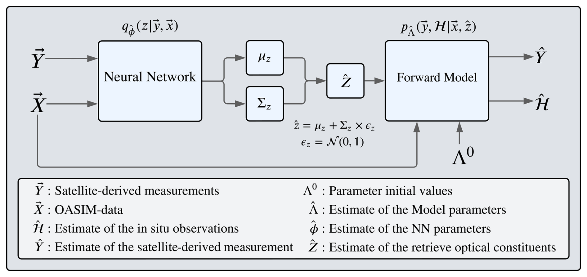
Figure 2 Diagram of the variational Bayes framework, adapted for the inversion problem, where the estimated $\widehat{Z}$ is retrieved using a parameterized probabilistic function $q_{\mathit{\varphi }}\left(\mathit{z}\right|\mathit{y},\mathit{x})$, which for our case is a feed-forward neural network (diagram in Fig. 3), and whose parameters ϕ are learned simultaneously to the parameters Λ, which are the parameters from the forward model.

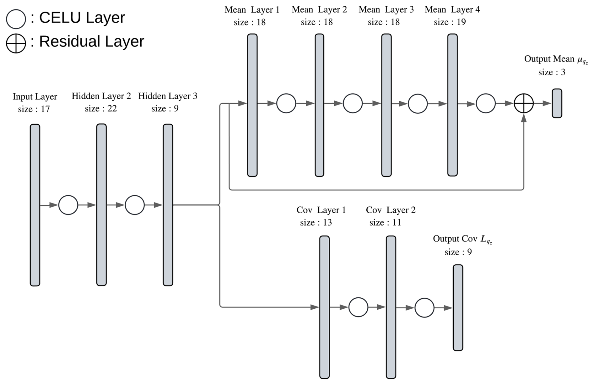
Figure 3 Diagram of the neural network (Soto, 2025) used as the parameterized probabilistic function $q_{\mathit{\varphi }}\left(\mathit{z}\right|\mathit{x},\mathit{y})$. It is composed of three sections: the first two hidden layers reduce the dimensionality of the input layer by projecting it into the space of the in situ observations. The output of the second layer is the input of the layers that learn the mean value of the latent variable ${\mathit{\mu }}_{q_z}$ and those that learn the components of the square root of the covariance matrix ${\mathbf{\Sigma }}_{q_z}={\mathbf{L}}_{q_z}^T{\mathbf{L}}_{q_z}$. The dimension of the hidden layers and the number of hidden layers are tuned using Ray Tune (Liaw et al., 2018).

5 Results

The results are divided into four parts: the first part focuses on the Bayesian retrieval of the optically active constituents at the surface of the sea and the uncertainty estimation, the second part discusses the parameter optimization, the third part compares the Bayesian outputs with the variational Bayes approach, and the last part presents a comparison with a state-of-the-art algorithm for satellite sea surface chlorophyll a estimation.

5.1 Bayesian inversion

We performed the Bayesian inversion from 2005 to 2013. As shown in Fig. 4, the retrieved sea surface chlorophyll manages to reproduce the interannual variability, including the spring algal blooms. The reported uncertainty serves as an estimate of the average expected discrepancy between retrieved data and in situ measurements, not only for chlorophyll observations but also for the downward light attenuation coefficient and particulate backward-scattering coefficient observations. We tested the performance of the inversion with a random sample consisting of 10 % of the days with observations. The root mean square error between the observations and the inverted data was computed (see Table D1), as well as the Spearman rank correlation coefficient (ρ; Table D2) and the relative median absolute deviation (rMAD; Table D3).

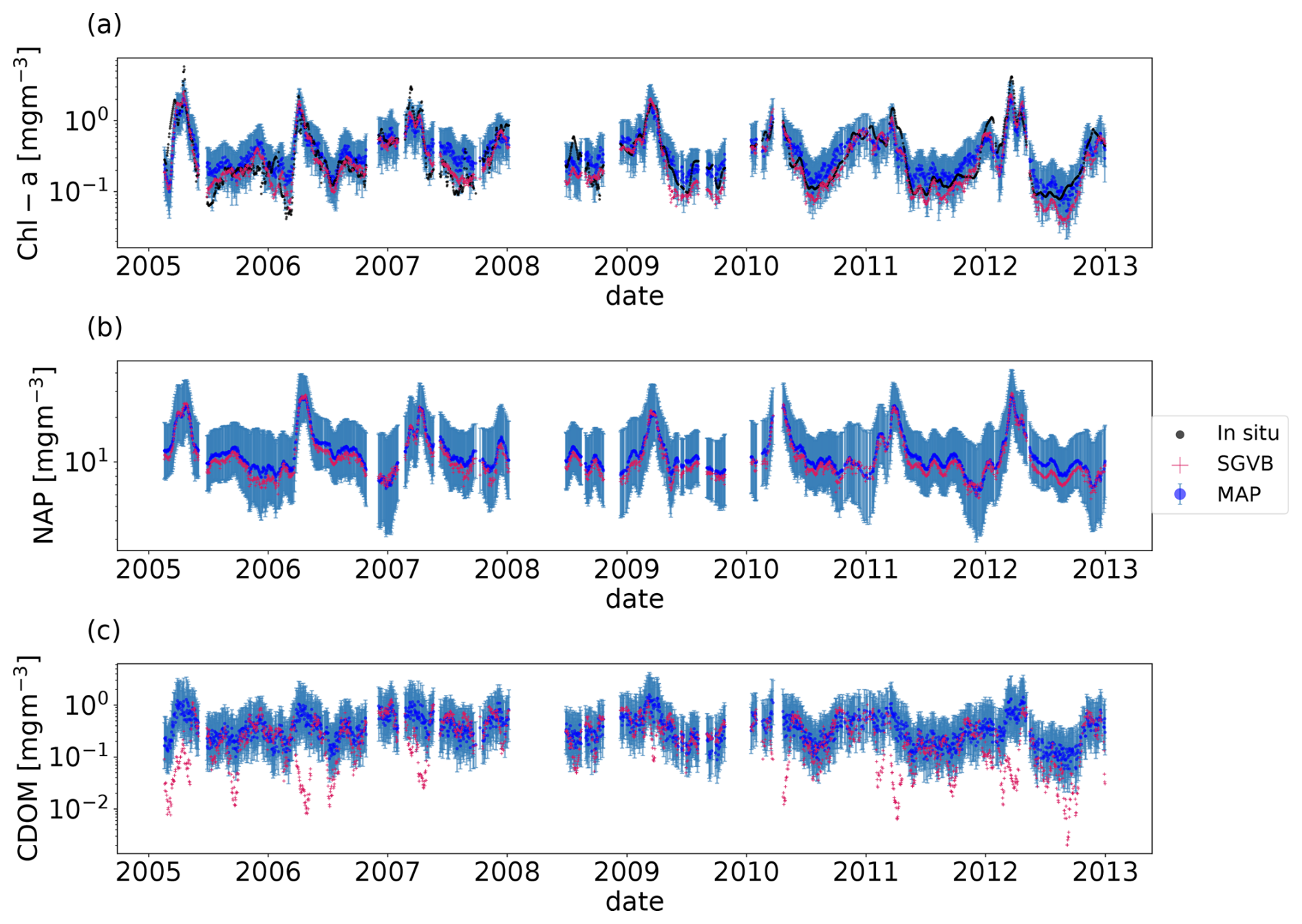
Figure 4 Time series for the chlorophyll α (a), non-algal particles (b), and colored dissolved organic matter (c). For all the timelines, the black points are the in situ observations from the BOUSSOLE buoy, the blue points are the MAP output with uncertainty (blue shadow) using the optimal parameters from the SGVB-based framework algorithm, and the red points are the output of the SGVB-based framework.

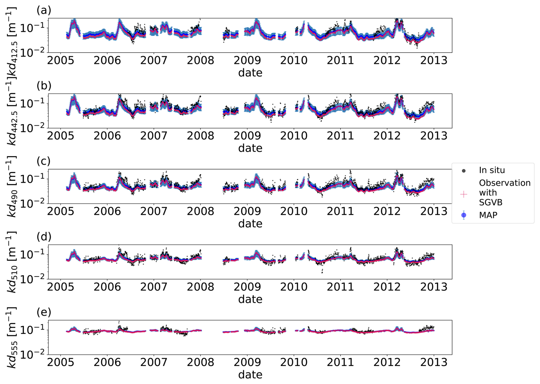
Figure 5 Time series for the downward light attenuation coefficient (k_d(λ)), with wavelengths λ=412.5 (a), λ=442.5 (b), λ=490 (c), λ=510 (d), and λ=555 (e). For all the timelines, the black points are the in situ observations from the BOUSSOLE buoy, the blue points are the MAP output with uncertainty (blue shadow) using the optimal parameters from the SGVB-based framework algorithm, and the red points are the observation operator computed using the output of the SGVB-based framework.

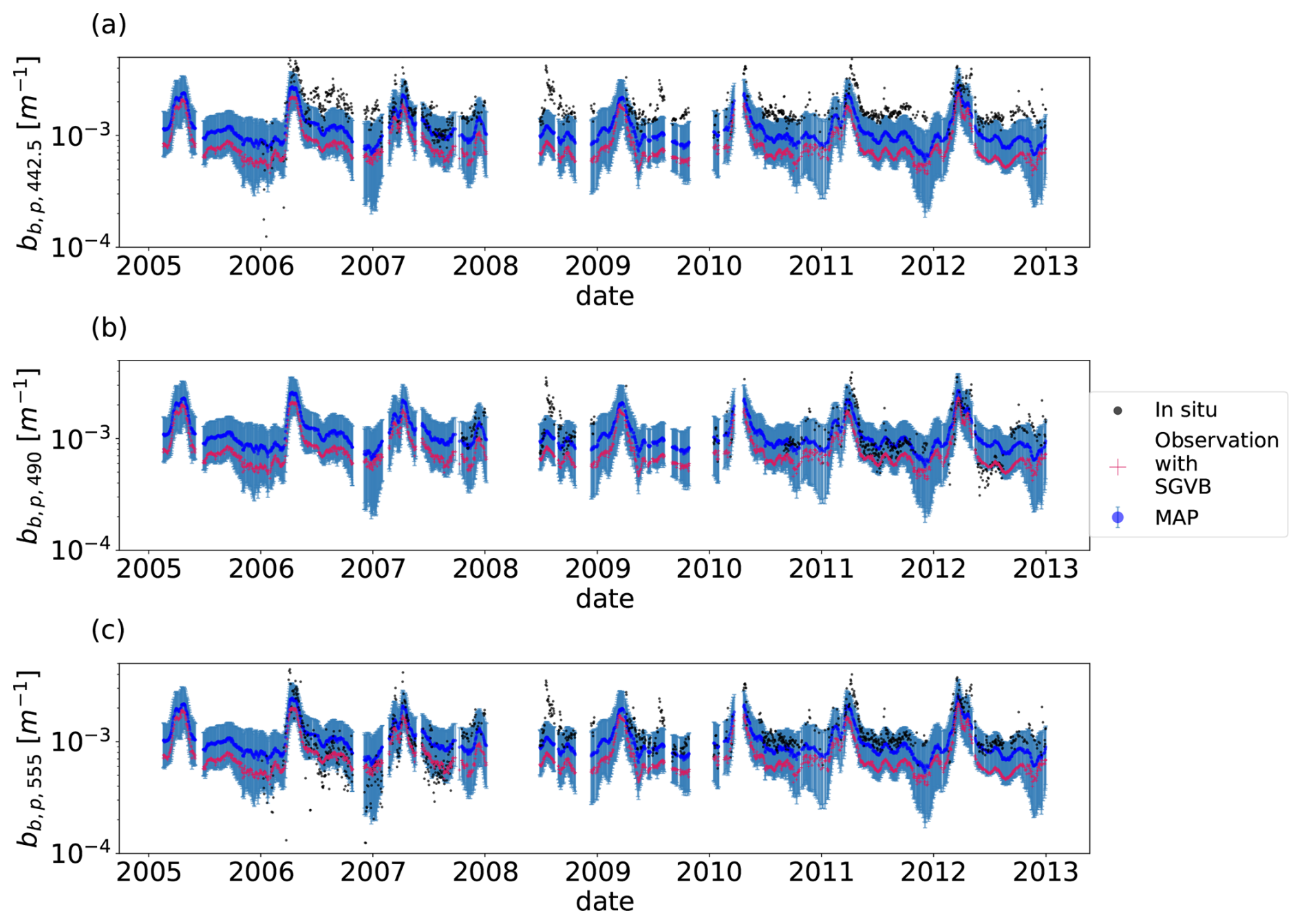
Figure 6 Time series for particulate backward-scattering coefficient for the wavelengths λ=442.5 (a), λ=490 (b), and λ=555 (c). For all the timelines, the black points are the in situ observations from the BOUSSOLE buoy, the blue points are the MAP output with uncertainty (blue shadow) using the optimal parameters from the SGVB-based framework algorithm, and the red points are the observation operator computed using the output of the SGVB-based framework.

Figure 7 shows a comparison between the true posterior distribution, sampled using the Metropolis–Hasting algorithm, and the estimated one using the linear approximation for the inversion of the remote sensing reflectance of 18 February 2005. The true posterior means and standard deviations are closely approximated by the linearization, even if the forward function is highly nonlinear. This result is closely related to the choice of the prior α𝟙=1.3𝟙, computed as explained in Sect. C, since it is a strongly informative prior. We can study the effect of the prior by computing the inverse of the Fisher information matrix, since the Cramér–Rao bound states that the variance in the MLE is always higher than or equal to this quantity:

$$\begin{array}{}\text{(31)}& \text{Var}\left[\widehat{\mathit{\psi }}\right]\ge {\displaystyle \frac{\mathrm{1}}{\mathbf{I}\left(\mathit{\psi }\right)}},\end{array}$$

where $\widehat{\mathit{\psi }}$ is an unbiased estimator of a random parameter ψ, and I(ψ) is the Fisher information matrix, defined as

$$\begin{array}{}\text{(32)}& \mathbf{I}\left(\mathit{\psi }\right)=-\mathbb{E}\left[{\displaystyle \frac{d^{\mathrm{2}}\mathcal{L}(X;\mathit{\psi })}{d{\mathit{\psi }}^{\mathrm{2}}}}\right],\end{array}$$

where ℒ(X;ψ) is the likelihood of a random variable X with parameters ψ (Cramér, 1999). For our case, the Fisher information matrix is equal to

$$\begin{array}{}\text{(33)}& \mathbf{I}\left(\mathrm{\Lambda }\right)={\mathbf{K}}^T{\mathbf{\Sigma }}_{\mathit{ϵ}}^{-\mathrm{1}}\mathbf{K},\end{array}$$

which is equal to the inverse of Eq. (19) without the effect of the prior. To quantify the effect of the prior, we divided the average Frobenius norm of the inverse of the Fisher information matrix $\left|\right|\mathrm{1}/\mathbf{I}\left(\mathrm{\Lambda }\right)|{|}_{\mathrm{2},\mathrm{2}}$ by the retrieved covariance matrix $\left|\right|{\mathbf{\Sigma }}_{{\stackrel{\mathrm{̃}}{z}}^d}|{|}_{\mathrm{2},\mathrm{2}}$, obtaining the value of 42.9, which means that the prior reduces the uncertainty of the MLE by a factor of 42. On the other hand, this highly informative prior is a reasonable prior, since it states that most of the chlorophyll concentration should be within values lower than $\text{exp}({\mathit{\mu }}_z+\mathrm{2}{\mathit{\sigma }}_{\stackrel{\mathrm{̃}}{z}})=\text{exp}\left(\mathrm{2.6}\right)=\mathrm{13.46}$ mg m⁻³ and higher than $\text{exp}({\mathit{\mu }}_z-\mathrm{2}{\mathit{\sigma }}_{\stackrel{\mathrm{̃}}{z}})=\text{exp}(-\mathrm{2.6})=\mathrm{0.07}$ mg m⁻³.

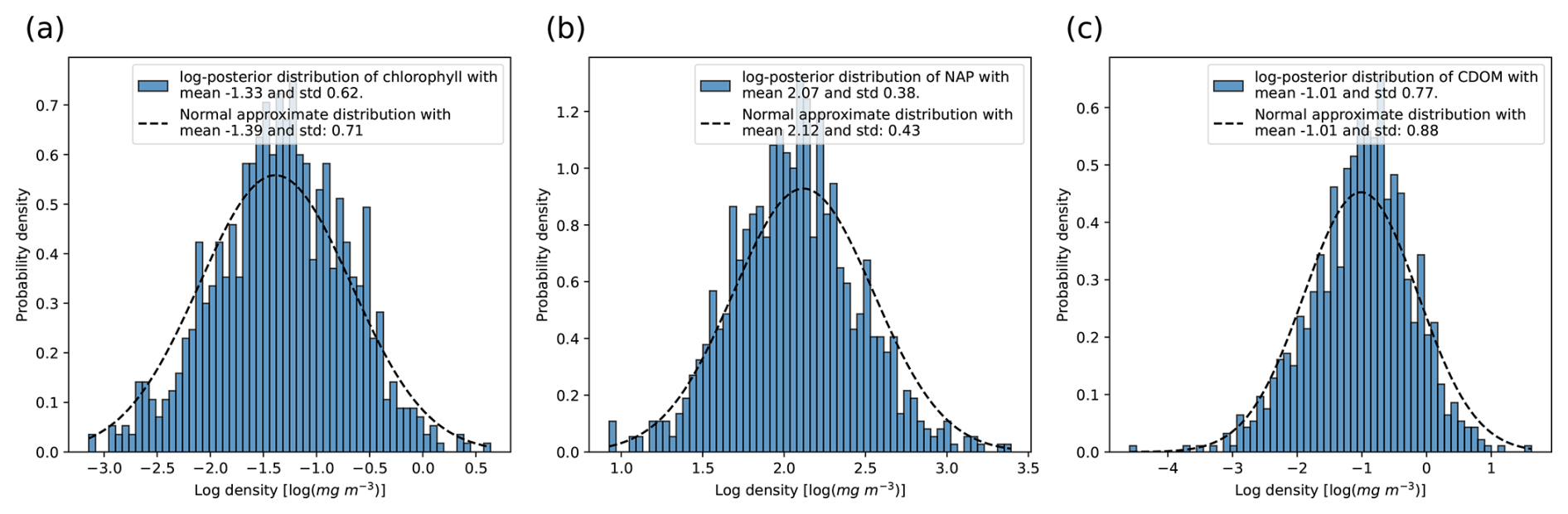
Figure 7 Comparison between the true posterior distribution (see Eq. 16) and the approximate posterior by following the algorithm in Algorithm 1 for the log-posterior distribution of (a) chlorophyll α, (b) non-algal particles, and (c) colored dissolved organic matter for the first day of the training data (18 February 2005). The true posterior (in blue) was sampled using the Metropolis–Hasting algorithm (see Algorithm 2), while the normal approximation (dashed line) was derived by linearization of the forward model around the MAP estimate.

5.2 Optimization of the forward model parameters

As described in Sect. 4.3.1, we tuned 24 parameters, multiplying them by 14 perturbation factors, to minimize the distance between the retrieved quantities and observation data. We are interested in the optimized parameter values and the uncertainties. If any of our final parameterizations are to be used in future work, it is important to note that we find optimal parameters that are representative of data from different seasons. For this reason, we present a sensitivity analysis where we can appreciate the annual variability in the sensitivity. Parameters with high variability may need special considerations for models that use different parameterizations for different seasons.

Following Carmichael et al. (1997), the sensitivity of the remote sensing reflectances, downward light attenuation coefficient, and backward-scattering coefficient can be computed by calculating the partial derivative with respect to the different parameters ($\partial R_{\text{RS}}/\partial {\mathit{\delta }}_i$, $\partial kd/\partial {\mathit{\delta }}_i$, $\partial b_{b,\mathrm{p}}/\partial {\mathit{\delta }}_i$), named the local sensitivity coefficients, and normalized with respect to the sensitivity coefficient ($R_{\text{RS}}/{\mathit{\delta }}_i$, $kd/{\mathit{\delta }}_i$, $b_{b,\mathrm{p}}/{\mathit{\delta }}_i$) to the obtained adimensional quantities. The results can be observed in Fig. 8.

We noticed that R_RS and b_b,p share a strong variability in the sensitivity with respect to the backward-scattering coefficient of phytoplankton, b_b,phy; the backscattering-to-scattering ratio of NAP, b_r,NAP; and the parameters ${\mathrm{\Theta }}_{\text{chla}}^{\text{min}},{\mathrm{\Theta }}_{\text{chla}}^{\mathrm{0}},\mathit{\beta }$, and σ, which form part of the chla : C ratio relation described in Eq. (3). This agrees with the seasonal variability in the abundance of the different phytoplankton functional types (Lazzari et al., 2012) and the variability in concentrations of pollution (Bodin et al., 2004). With this observation, we expect that using only one set of parameters for the full year would result in suboptimal predictions. Nevertheless, we proceed to find the optimal parameters that describe the full historical dataset.

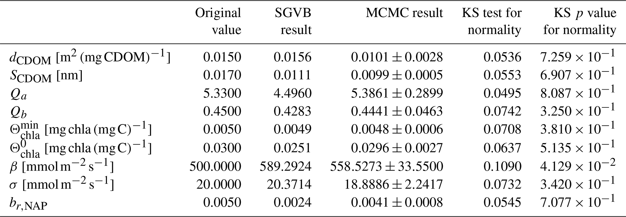
To do so, we performed an MCMC algorithm as described in Sect. 4.3.1. An example of the distribution obtained for each parameter can be observed in Fig. 9. The original values and the mean and standard deviation for the λ-dependent parameters can be seen in Fig. 10. Finally, the original values and the statistics obtained using the MCMC algorithm for the λ-independent parameters can be seen in Table 4.

Table 4 Original values and final values obtained using the SGVB estimator, as well as the mean, standard deviation, and Kolmogorov–Smirnov test coefficient for the sampling with the Metropolis–Hasting algorithm for the λ-independent parameters.

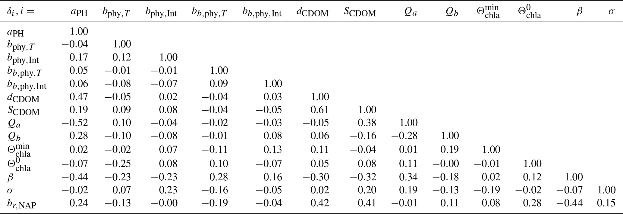
For completeness, we also computed the covariance matrix between the perturbation factors δ_i, which can be seen in Table 5.

Table 5 Correlation matrix between the perturbation factors δ_i, computed using the samples from the Metropolis–Hasting algorithm.

The main result of the new parameterization is a decrease in the root mean square error (RMSE) between the test data of sea surface chlorophyll observations and inverted values. A key aspect to note is that the MLE computed using the training data can present overfitting; for this reason, we had to use early stopping during the alternate minimization step, and then we proceeded to use the mean value of the estimated posterior estimated with the MCMC samples. Since we observed a decrease in the RMSE (see Table D1) for the test data, we can say that the posterior mean is good for generalization.

5.3 Comparison between Bayesian retrievals and the variational Bayes approach

As described in Sect. 4.4, we used the SGVB estimator to find an optimal parameterization. The results can be appreciated in Table 4 and Fig. 10. Taking into account the uncertainty in the MCMC results and using the 95 % confidence interval, 22 of the 24 parameters perturbed with the SGVB estimator agree with the MCMC estimation, in the sense that the SGVB output is within the uncertainty range of the MCMC estimate. The two parameters with a high discrepancy between the two frameworks are Q_a, on average the most sensitive parameter concerning remote sensing reflectance, and b_r,NAP, one of the most sensitive parameters concerning particulate backward scattering.

To assess the performance of each set of parameters, we evaluated the MAP estimates of the optical constituents z given each set of parameters (MAP estimate obtained with the MCMC algorithm and the MLE obtained with the SGVB estimator) for the test dataset. Recall that this dataset was not used for any parameter tuning before, so these results serve as a confirmation of the robustness of the methods.

The main indicator is the sea surface chlorophyll observations, as they are the least noisy and scattered observation data. Based on the root mean square error (RMSE) and relative median absolute deviation (rMAD) between the measurements and retrieved estimates (Tables D1 and D3), both parameter sets improved the inversion results. However, the parameter set optimized using the SGVB estimator yielded the best performance.

The observations of the downward light attenuation coefficient and the particulate backward-scattering coefficient are much more scattered and noisy than those of chlorophyll, yet the SGVB parameters optimized all the model output matching observations, while the MCMC favored better outputs only for the k_d values. We speculate that this is due to overfitting, as the measurements of particulate backward scattering are highly scattered. Moreover, as particulate backward scattering is sensitive to b_r,NAP, the estimated value from the MCMC could be affected by the noise. In the case of NN training, we used mini-batch minimization, which may have helped us to find a parameter value that is better for generalization.

The SGVB estimator also provides an efficient way of computing estimates of the optical constituents z, which, by construction, are also consistent with the forward model, with optimal RMSE between measurements and estimates. Since they are computed with a neural network, the computational time outperforms the standard implicit inversion methods, required in cases where the expression of the RTE is too complicated to invert it analytically. For comparison, the estimated optical constituents $\widehat{\mathit{z}}$ using the SGVB estimator are shown in Figs. 4–6, and the statistics for the observation operator using these estimates are shown in Tables D1, D2, and D3.

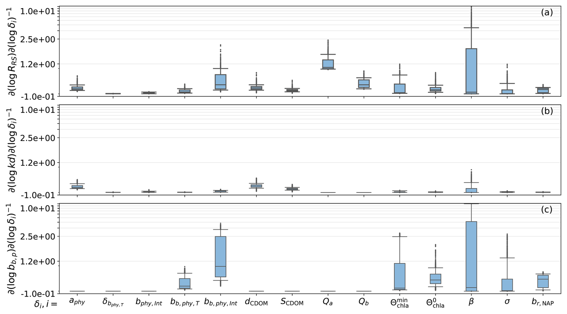
Figure 8 Sensitivity of (a) R_rs, (b) kd, and (c) b_b,p with respect to the perturbation factors δ_i evaluated at δ_i=1. The box plots represent the quartiles of the sensitivity for each day.

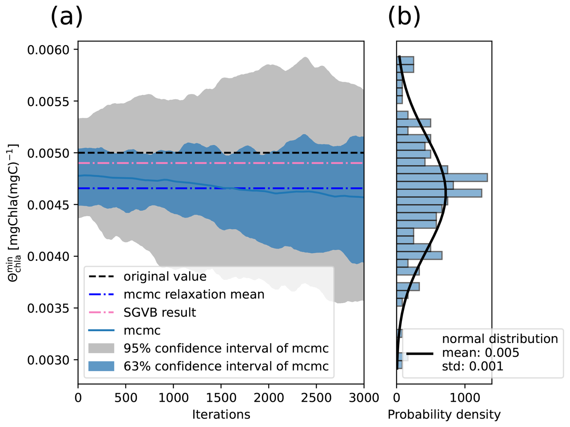
Figure 9 Result of the Metropolis–Hasting algorithm for the parameter ${\mathrm{\Theta }}_{\text{chla}}^{\text{min}}$ [mg chla (mg C)⁻¹], using the transition probability shown in Eq. (23), with initial conditions close to the value obtained after performing alternate minimization. (a) Evolution of the parameter after each iteration of the algorithm and (b) final probability density estimated as a Gaussian distribution.

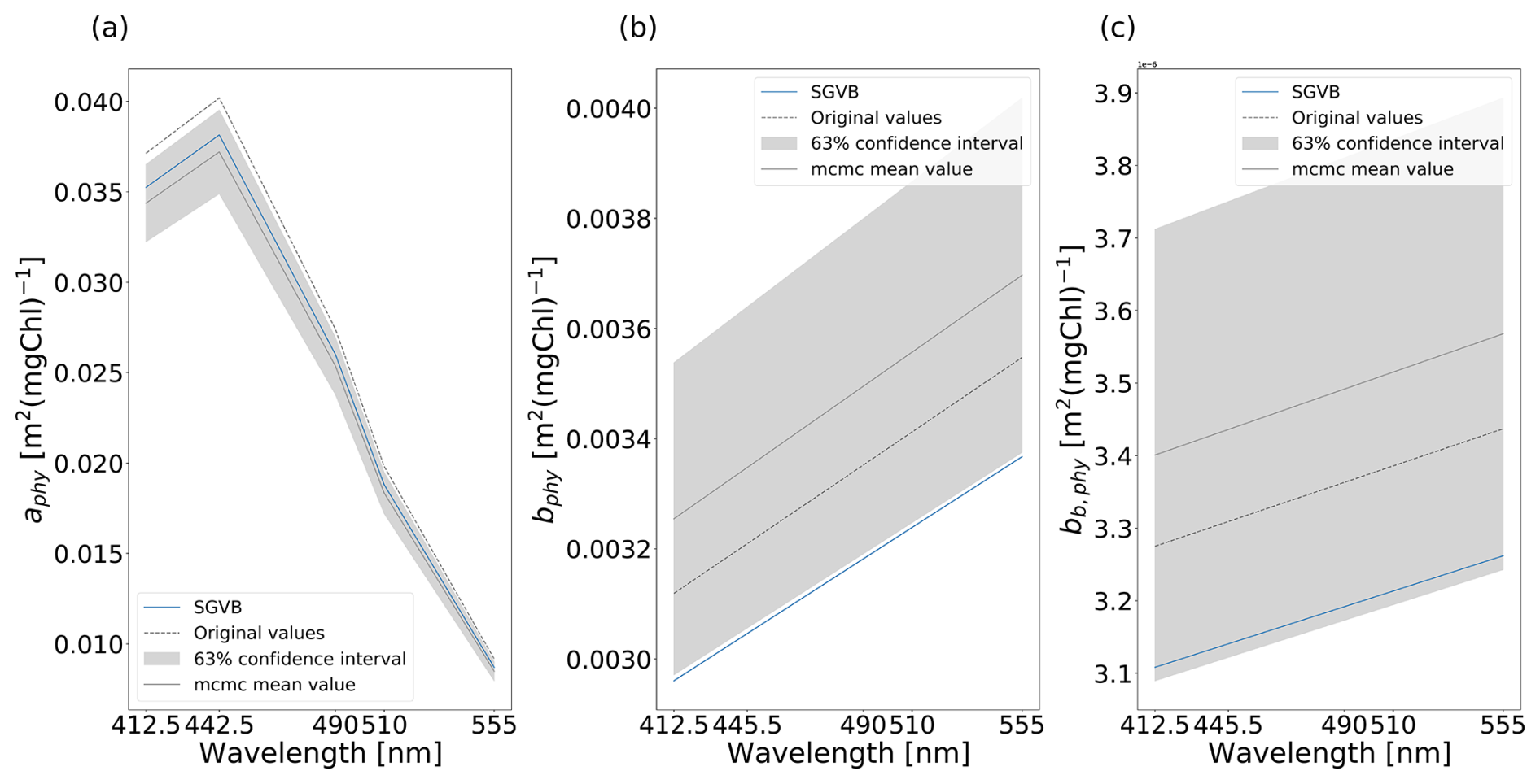
Figure 10 Original values (dashed line), final values using the SGVB-based framework (blue), and the mean and standard deviation (gray) for the λ-dependent parameter (a) absorption coefficient of phytoplankton a_phy(λ), (b) scattering coefficient of phytoplankton b_phy(λ), and (c) backward-scattering coefficient of phytoplankton b_b,phy(λ).

We observe that the standard Bayesian estimate and that using the SGVB estimator are close to each other (Fig. 4), since the SGVB estimator outputs are within the uncertainty range of the Bayesian estimate. Differences between both could be due to model errors, since the SGVB estimator requires approximating the posterior with a parameterized probability distribution, in our case, a neural network, or differences between the training algorithms. The variational Bayes method also estimates the covariance matrix between the latent variables Z; nevertheless, since the uncertainty was underestimated, we only plotted the mean values.

5.4 Comparison with satellite products

To assess the validity of the results with respect to state-of-the-art algorithms, we compared the capability of the DIIM system in a wider region of the northwestern Mediterranean Sea, characterized by highly dynamic regimes of vertical mixing during the spring period and stratification during summer. The comparison is carried out using additional in situ data (not used in the calibration of DIIM), based on high-performance liquid chromatography (HPLC;, Di Biagio et al., 2025), and a standard ocean color retrieval approach used by the Copernicus Marine Service, MedOC4.2020 (Colella et al., 2025). The latter approach is based on a calibrated nonlinear regression of the maximum R_rs in the wavelengths at 443, 490, and 510 nm, normalized over R_rs at 555 nm:

$$\begin{array}{}\text{(34)}& \begin{array}{rl}& {\text{chlorophyll}}_{\text{satellite}}={\mathrm{10}}^{(a_{\mathrm{0}}+a_{\mathrm{1}}X+a_{\mathrm{2}}{X}^{\mathrm{2}}+a_{\mathrm{3}}{X}^{\mathrm{3}}+a_{\mathrm{4}}{X}^{\mathrm{4}})},\\ & X={\log }_{\mathrm{10}}\left({\displaystyle \frac{\text{max}(R_{\text{rs},\mathrm{443}},R_{\text{rs},\mathrm{490}},R_{\text{rs},\mathrm{510}})}{R_{\text{rs},\mathrm{555}}}}\right),\\ & a_{\mathrm{0}}=\mathrm{0.327},a_{\mathrm{1}}=-\mathrm{2.994},a_{\mathrm{2}}=\mathrm{2.722},\\ & a_{\mathrm{3}}=-\mathrm{1.226},a_{\mathrm{4}}=-\mathrm{0.568}.\end{array}\end{array}$$

To do so, we computed the surface downward direct and scattered irradiance as described in Lazzari et al. (2021) for the days and places where in situ measurements were taken (see Fig. 11a). We chose a square of 4°×4° close to the BOUSSOLE buoy for the samples and selected those with a bathymetry lower than 200 m and performed at less than 10 m deep. For the remote sensing reflectance (CMEMS, 2023), we used an average of 5 d, with a ∼5 km window around the points. Finally, we used the SGVB estimator to invert the remote sensing reflectance and estimate the chlorophyll concentration. The outputs can be observed in Fig. 11.

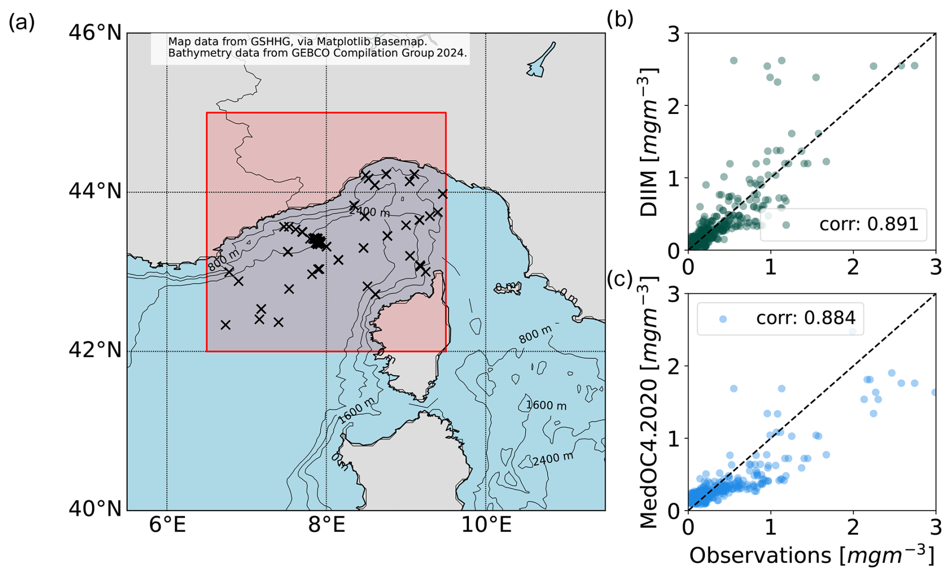
Figure 11 (a) Region in red and locations with in situ measurements (x) for the comparison between (b) the inverted values of chlorophyll a using the SGVB estimator and (c) a standard ocean color retrieval approach used with the Copernicus Marine Service (Colella et al., 2025).

Results are consistent between in situ data and inversion models, suggesting that the present approach is applicable over spatially heterogeneous conditions.

6 Discussion

In the last few years, there has been an increasing number of applications of neural networks in Earth sciences, including forecasts of the El Niño–Southern Oscillation (ENSO) using historical simulations and convolutional neural networks (Ham et al., 2019), fusion of satellite data (Chapman and Charantonis, 2017; Denvil-Sommer et al., 2019; Bocquet et al., 2020), classification of regions in the ocean (Richardson et al., 2003; Saraceno et al., 2006), determination of drivers of net primary productivity using self-organizing maps (Lachkar and Gruber, 2012), reconstruction of oceanographic variables (Martinez et al., 2020; Pietropolli et al., 2022), classification of the anomalies in water-leaving radiance (Mustapha et al., 2014), data reconstruction (Manucharyan et al., 2021; George et al., 2021), inversion of oceanographic variables (Brajard et al., 2006; Irrgang et al., 2019; Dessailly, 2012), pattern recognition (Maze et al., 2017; Jones et al., 2019; Boehme and Rosso, 2021; Desbruyères et al., 2021), forecasts imposing physical constraints (De Bézenac et al., 2019; Erichson et al., 2019), and increasing the resolution of modeling (Barthélémy et al., 2022), among others.

Our work makes use of a neural network to approximate the posterior probability distribution of optical constituents in the sea by employing the SGVB estimator. As described in Sect. 4.4.1, we maximize the ELBO loss function, which simultaneously optimizes the forward model by finding the MLE of the parameters, deriving in situ biogeochemical parameters for reflectance observations, linking the neural network procedure to an interpretable model. As stated by Kingma and Welling (2022), this approach is especially useful to infer intractable posteriors and to find the MLE of the forward model parameters, a situation commonly encountered in data assimilation problems, where the number of parameters to optimize makes the problem intractable. This work serves as a test bed, comparing the more traditional Bayesian inference approach with the results obtained with the SGVB estimator, and presenting a pointwise observation operator for the active optical constituents chlorophyll, NAP, and CDOM.

Our results with the SGVB estimator underestimated the uncertainty in the optical constituents, a computation that is of crucial importance for multiple applications, like objective comparison of simulations against observations and efficient assimilation of data with methods like Kalman filters, among others (Brankart et al., 2012). A further analysis is needed to assess the effect of each term of the loss function on the NN covariance matrix, as well as to determine whether the inclusion of a regularization term affects the uncertainty estimation. At the moment, the requirement of reliable uncertainty estimations leads us to use only the pointwise estimate of the neural network. Furthermore, we explored the Bayesian approach, approximating the final posterior distribution of the optical constituents, $p_{\mathrm{\Lambda }}\left(\mathit{z}\right|\mathit{y},\mathit{x})$, with a Gaussian probability distribution. This method returns estimates with reliable uncertainty estimations that can be used in real operational systems.

In particular, in addition to the optical constituents, we aimed to find the optimal model with respect to all the in situ observations for the entire period. This ambitious goal made the final results suboptimal for some individual measurements. For example, Salama and Verhoef (2015) used a similar forward model to estimate the downward light attenuation coefficient at a wavelength of 490 nm, kd(490), at different depths, obtaining an rMAD of 11.84 %, while our results using the MCMC parameters presented an rMAD value of 21 %. We noticed that by optimizing only one in situ measurement, we could find a set of parameters that made that measurement more precise. Nevertheless, we decided to use the parameters presented to balance the global accuracy. For example, in terms of the rMAD of the remote sensing reflectance at a wavelength of 490 nm, R_rs(490), we obtained an rMAD value of 1.8 %, outperforming previous works.

Our approach also differs from that of other work on Bayesian estimation of optical constituents (Gordon and Boynton, 1997; Boynton and Gordon, 2000; Michalopoulou et al., 2009; Erickson et al., 2023), since we employ a three-stream model, derived from the radiative transfer model (Dutkiewicz et al., 2015), and use it to derive the in situ observations for all available wavelengths. This feature allows scientists to understand the automatic learning process in terms of meaningful physical parameters.

The approach can be extended in different directions, particularly through the addition of more optical constituents, which will be facilitated once information from the new satellite missions Hyperspectral Precursor of the Application Mission (PRISMA), with 12 nm spectral resolution ranging from 400 to 2500 nm, and the Plankton, Aerosol, Cloud, Ocean Ecosystem (PACE), with 5 nm resolution ranging from 350 to 890 nm, is used as input to the system, or through the addition of the forward model terms that take into account the interaction with the sea floor, which is crucial for the analysis of shallow waters.

7 Conclusions

By utilizing the Bayes theorem and linearizing the forward function, we achieved the inversion of the optical constituents, with an estimate of the uncertainty. The latter is fundamental for the assimilation of remote sensing reflectance.

By using an MCMC algorithm, we computed a set of parameters that optimized the forward model and showed that the method was robust by obtaining coherent values with the SGVB estimator. Moreover, the variational Bayes framework can be used as an alternative to find pointwise estimates of optimal parameters and also as an efficient way of computing pointwise estimates of the optical constituents.

Regarding the computational advantages of the SGVB estimator, as long as the uncertainty is not required, it is the best option to estimate the optical constituents in operational systems, since, after training, the evaluation of the neural network is much faster than the iterative minimization (an effect known as amortization). Nevertheless, the posterior probability learned by the neural network underestimates the uncertainty in the result, which makes the MAP algorithm preferable when the uncertainty is a requirement. Since the computational time for the MAP estimate depends on the initial conditions, we proposed using the SGVB estimates as initial conditions for the MAP algorithm, which, based on experiments with our current implementation, we found to be capable of reducing the number of steps by more than 50 %.

For future work, it would be important to apply and verify the accuracy of the approach with more optical constituents and to test remote sensing reflectance assimilation in a biogeochemical model.

Appendix A

In this section, we expand the solution of Eq. (1) subject to the boundary conditions in Eq. (6), under the homogeneity assumption. First, for simplicity, we re-write Eq. (1) as

$$\begin{array}{}\text{(A1)}& \begin{array}{rl}{\displaystyle \frac{\mathrm{d}{E}_{\text{dir}}(h,\mathit{\lambda })}{\mathrm{d}h}}=& -c_d\left(\mathit{\lambda }\right)E_{\text{dir}}(h,\mathit{\lambda }),\\ {\displaystyle \frac{\mathrm{d}{E}_{\text{dif}}(h,\mathit{\lambda })}{\mathrm{d}h}}=& -C_s\left(\mathit{\lambda }\right)E_{\text{dif}}(h,\mathit{\lambda })+B_u\left(\mathit{\lambda }\right)E_u(h,\mathit{\lambda })\\ & +F_d\left(\mathit{\lambda }\right)E_{\text{dir}}(h,\mathit{\lambda }),\\ {\displaystyle \frac{\mathrm{d}{E}_{\text{u}}(h,\mathit{\lambda })}{\mathrm{d}h}}=& -B_s\left(\mathit{\lambda }\right)E_{\text{dif}}(h,\mathit{\lambda })+C_u\left(\mathit{\lambda }\right)E_u(h,\mathit{\lambda })\\ & -B_d\left(\mathit{\lambda }\right)E_{\text{dir}}(h,\mathit{\lambda })\\ \text{subject to}& \\ E_{\text{dir}}(\mathrm{0},\mathit{\lambda })=& E_{\text{dir}}^{\text{OASIM}}(\mathrm{0},\mathit{\lambda }),\\ E_{\text{dif}}(\mathrm{0},\mathit{\lambda })=& E_{\text{dif}}^{\text{OASIM}}(\mathrm{0},\mathit{\lambda }),E_{\text{u}}(\mathrm{\infty },\mathit{\lambda })=\mathrm{0},\end{array}\end{array}$$

where

$$\begin{array}{}\text{(A2)}& \begin{array}{rl}{c}_d\left(\mathit{\lambda }\right)& ={\displaystyle \frac{a\left(\mathit{\lambda }\right)+b\left(\mathit{\lambda }\right)}{\cos \mathit{\theta }}},\\ C_s\left(\mathit{\lambda }\right)& ={\displaystyle \frac{a\left(\mathit{\lambda }\right)+r_s{b}_b\left(\mathit{\lambda }\right)}{v_s}},\\ B_u\left(\mathit{\lambda }\right)& ={\displaystyle \frac{r_u{b}_b\left(\mathit{\lambda }\right)}{v_u}},\\ F_d\left(\mathit{\lambda }\right)& ={\displaystyle \frac{b\left(\mathit{\lambda }\right)-r_d{b}_b\left(\mathit{\lambda }\right)}{\cos \mathit{\theta }}},\\ B_s\left(\mathit{\lambda }\right)& ={\displaystyle \frac{r_s{b}_b\left(\mathit{\lambda }\right)}{v_s}},\\ C_u\left(\mathit{\lambda }\right)& ={\displaystyle \frac{a\left(\mathit{\lambda }\right)+r_u{b}_b\left(\mathit{\lambda }\right)}{v_u}},\\ B_d\left(\mathit{\lambda }\right)& ={\displaystyle \frac{r_d{b}_b\left(\mathit{\lambda }\right)}{\cos \mathit{\theta }}}.\end{array}\end{array}$$

Equation (A1) is a linear system of ordinary differential equations, which can be solved by first solving the equation for E_dir(h,λ), followed by solving the system of equations for E_dif(h,λ) and E_u(h,λ), taking the solution of E_dir(h,λ) as the inhomogeneous part of the system of equations. The final expression is

$$\begin{array}{}\text{(A3)}& \begin{array}{rl}{E}_{\text{dir}}(h,\mathit{\lambda })& =E_{\text{dir}}^{\text{OASIM}}(\mathrm{0},\mathit{\lambda })e^{-h{c}_d},\\ E_{\text{dif}}(h,\mathit{\lambda })& =c^{+}{e}^{-k^{+}h}+x_{\text{dif}}{E}_{\text{dir}}(h,\mathit{\lambda }),\\ E_u(h,\mathit{\lambda })& =c^{+}{r}^{+}{e}^{-k^{+}h}+y_{\text{u}}{E}_{\text{dir}}(h,\mathit{\lambda }),\end{array}\end{array}$$

where

$$\begin{array}{}\text{(A4)}& \begin{array}{rl}{c}^{+}& =E_{\text{dif}}^{\text{OASIM}}(\mathrm{0},\mathit{\lambda })-x{E}_{\text{dir}}^{\text{OASIM}}(\mathrm{0},\mathit{\lambda }),\\ k^{+}& =D-C_u,\\ r^{+}& ={\displaystyle \frac{B_s}{D}},\\ D& ={\displaystyle \frac{\mathrm{1}}{\mathrm{2}}}\left(C_s+C_u+\sqrt{{\left(C_s+C_u\right)}^{\mathrm{2}}-\mathrm{4}{B}_s{B}_u}\right),\\ x& ={\displaystyle \frac{\left(-(C_u+c_d)F_d-B_u{B}_d\right)}{(c_d-C_s)(c_d+C_u)+B_s{B}_u}},\\ y& ={\displaystyle \frac{\left(-B_s{F}_d+(-C_s+c_d)B_d\right)}{(c_d-C_s)(c_d+C_u)+B_s{B}_u}}.\end{array}\end{array}$$

In the case when the expression $(c_d-C_s)(c_d+C_u)+B_s{B}_u=\mathrm{0}$, then the expression for c⁺ has to be changed to $c^{+}=E_{\text{dif}}^{\text{OASIM}}(\mathrm{0},\mathit{\lambda })$.

Appendix B: Tuning of the hyperparameter α

As seen in Sect. 4, the final covariance matrix for the retrieved ${\stackrel{\mathrm{̃}}{Z}}^{*}$ depends on the hyperparameter α by the equation Σ_z=α𝟙. We selected the value of α to fulfill two criteria: the retrieved ${\stackrel{\mathrm{̃}}{Z}}^{*}$ should be robust to α, meaning small changes in α should not change the retrieved quantity, and the estimated uncertainty has to be close to the discrepancy between the retrieved data and in situ observations.

To this end, we defined the error in the forward model ${\mathit{ϵ}}_{R_{\text{rs}}}\left(\mathit{\alpha }\right)$ as the root mean square difference between the satellite remote sensing reflectance and that predicted by the model. The aim is to make this quantity robust to α.

We also defined the error between the predicted uncertainty and the actual discrepancy between the model and data ${\mathit{ϵ}}_{{\mathit{\delta }}_{\text{chla}}}\left(\mathit{\alpha }\right)$, where the predicted uncertainty is estimated as the mean value of the standard deviation of the predicted chla^MODEL, and the discrepancy between the model and data is estimated as the root mean square difference between chla^OBS and chla^MODEL.

We computed ${\mathit{ϵ}}_{R_{\text{rs}}}\left(\mathit{\alpha }\right)$ and ${\mathit{ϵ}}_{{\mathit{\delta }}_{\text{chla}}}\left(\mathit{\alpha }\right)$ for different values of α until the curve ${\mathit{ϵ}}_{R_{\text{rs}}}\left(\mathit{\alpha }\right)$ flattens. With the errors computed, we rescaled the error functions ${\mathit{ϵ}}_{R_{\text{rs}}}\left(\mathit{\alpha }\right)$ and ${\mathit{ϵ}}_{{\mathit{\delta }}_{\text{chla}}}\left(\mathit{\alpha }\right)$ between 0 and 1 in order to minimize both functions simultaneously by minimizing the following loss function:

$$\begin{array}{}\text{(B1)}& {\mathcal{L}}^{\mathit{\alpha }}=\stackrel{\mathrm{‾}}{{\mathit{ϵ}}_{R_{\text{rs}}}\left(\mathit{\alpha }\right)}+\stackrel{\mathrm{‾}}{{\mathit{ϵ}}_{{\mathit{\delta }}_{\text{chla}}}\left(\mathit{\alpha }\right)},\end{array}$$

where the line over the errors stands for the rescaling. Figure B1 shows the final value of α selected as a function of ${\mathit{ϵ}}_{R_{\text{rs}}}\left(\mathit{\alpha }\right)$, ${\mathit{ϵ}}_{{\mathit{\delta }}_{\text{chla}}}\left(\mathit{\alpha }\right)$, and ℒ^α.

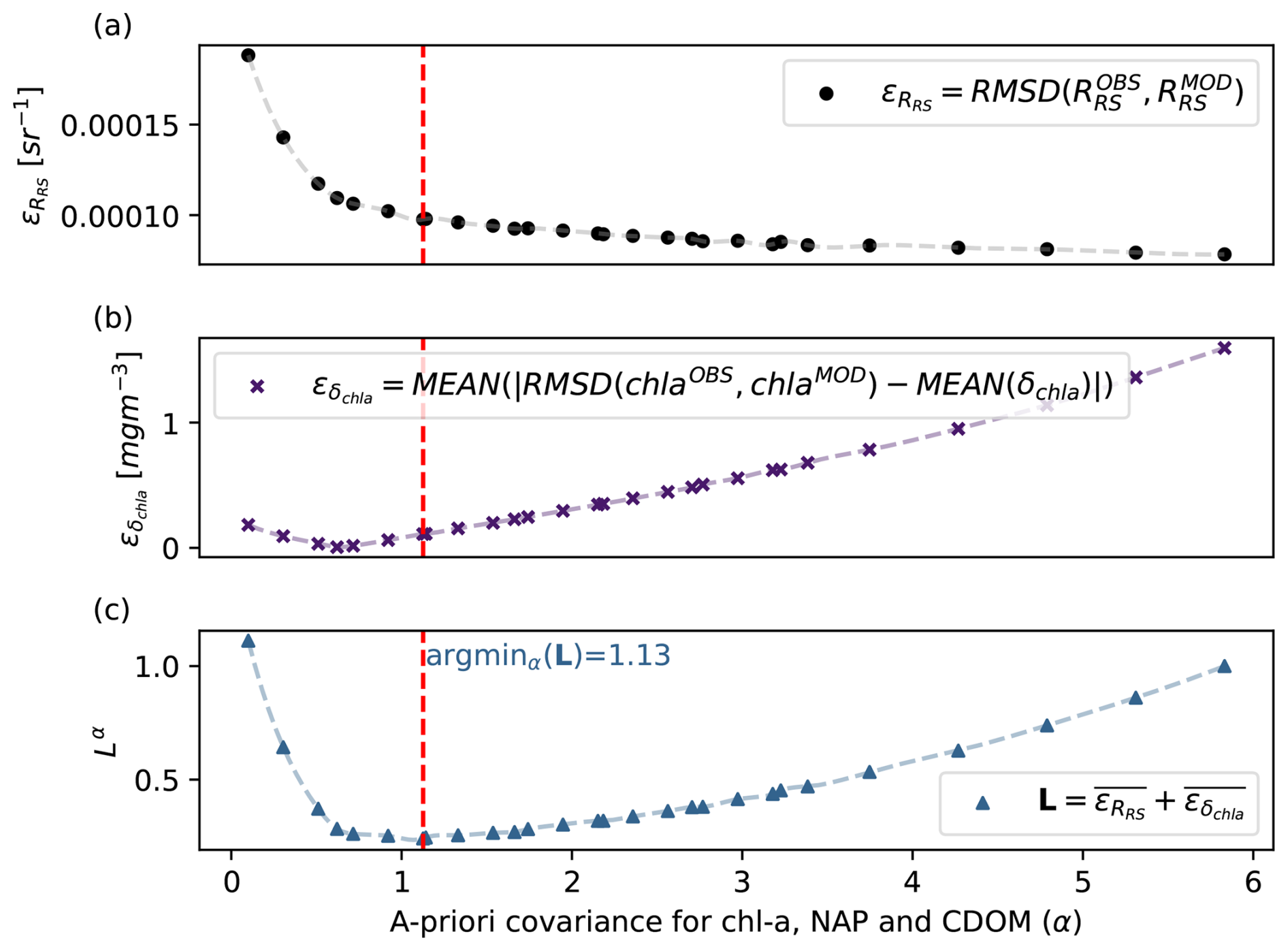
Figure B1 Illustration of how the hyperparameter α was chosen. Using a higher α decreases the root mean square difference between the remote sensing reflectance observed by the satellite and that obtained with the model (a) but increases the error between the predicted uncertainty and the actual discrepancy between the model and data (b). The value chosen was the one that minimized the ℒ^α loss function (c).

Appendix C

This section shows that ℒ_ELBO is a lower bound of the data log likelihood. First, we write the expression for the log likelihood by marginalizing over all possible values of the latent variable z:

$$\begin{array}{}\text{(C1)}& \log \left(p_{\mathrm{\Lambda }}\right(\mathit{y}\left)\right)=\log \left(\underset{\mathcal{Z}}{\int }{p}_{\mathrm{\Lambda }}\left(\mathit{y}\right|\mathit{z}\left)p\right(\mathit{z})\mathrm{d}\mathit{z}\right).\end{array}$$

Next we introduce the parameterized probability distribution q_ϕ(z|y):

$$\begin{array}{}\text{(C2)}& =\log \left(\underset{\mathcal{Z}}{\int }{p}_{\mathrm{\Lambda }}\left(\mathit{y}\right|\mathit{z}\left){\displaystyle \frac{q_{\mathit{\varphi }}\left(\mathit{z}\right|\mathit{y})}{q_{\mathit{\varphi }}\left(\mathit{z}\right|\mathit{y})}}p\right(\mathit{z})\mathrm{d}\mathit{z}\right).\end{array}$$

Finally, we use Jensen's inequality to find a lower bound for the log likelihood:

$$\begin{array}{ll}{\displaystyle }\ge & {\displaystyle }\underset{\mathcal{Z}}{\int }\log \left({\displaystyle \frac{p_{\mathrm{\Lambda }}\left(\mathit{y}\right|\mathit{z}\left)p\right(\mathit{z})}{q_{\mathit{\varphi }}\left(\mathit{z}\right|\mathit{y})}}\right)q_{\mathit{\varphi }}\left(\mathit{z}\right|\mathit{y})\mathrm{d}\mathit{z}\\ {\displaystyle }=& {\displaystyle }\underset{\mathcal{Z}}{\int }\log \left({\displaystyle \frac{p\left(\mathit{z}\right)}{q_{\mathit{\varphi }}\left(\mathit{z}\right|\mathit{y})}}\right)q_{\mathit{\varphi }}\left(\mathit{z}\right|\mathit{y})\\ {\displaystyle }& {\displaystyle }+\underset{\mathcal{Z}}{\int }\log \left(p_{\mathrm{\Lambda }}\right(\mathit{y}\left|\mathit{z}\right)\left)q_{\mathit{\varphi }}\right(\mathit{z}\left|\mathit{y}\right)\mathrm{d}\mathit{z}\\ {\displaystyle }=& {\displaystyle }-D_{\text{KL}}\left(q_{\mathit{\varphi }}\right(\mathit{z}\left|\mathit{y}\right)\left|\right|p\left(\mathit{z}\right))\\ {\displaystyle }& {\displaystyle }+{\mathbb{E}}_{q_{\mathit{\varphi }}\left(\mathit{z}\right|\mathit{y})}\left[\log \right(p_{\mathrm{\Lambda }}\left(\mathit{y}\right|\mathit{z}\left)\right)]\\ \text{(C3)}& {\displaystyle }=& {\displaystyle }{\mathcal{L}}_{\text{ELBO}}.\end{array}$$

The inequality is equal for the case $q_{\mathit{\varphi }}\left(\mathit{z}\right|\mathit{y})=p(\mathit{z}\left|\mathit{y}\right)$, the true posterior distribution, in which case ℒ_ELBO=log (p_Λ(y)). In other words, maximizing ℒ_ELBO equals maximizing the marginal log likelihood.

Appendix D

In this section, we include the root mean square error (RMSE), Pearson correlation coefficients (ρ), and relative median absolute deviation (rMAD) for all the measurements and observations, using the MAP estimates with unperturbed parameters, MAP estimate with parameters from the MCMC algorithm, MAP estimate with parameters from the SGVB estimator, and outputs from the SGVB estimator. All the quantities are computed using only the test data, which comprise 10 % of the data and were not used in the MCMC algorithm or in the training of the neural network. Finally, we include tables with the symbols used throughout this work.

Table D1 Root mean square error between satellite and in situ observations and the modeled data using the maximum a posterior (MAP) estimate with unperturbed parameters, optimized parameters with the MCMC algorithm, optimized parameters with the SGVB-based framework, and data modeled purely with the SGVB-based framework. Note that a log transform was performed before the computations.

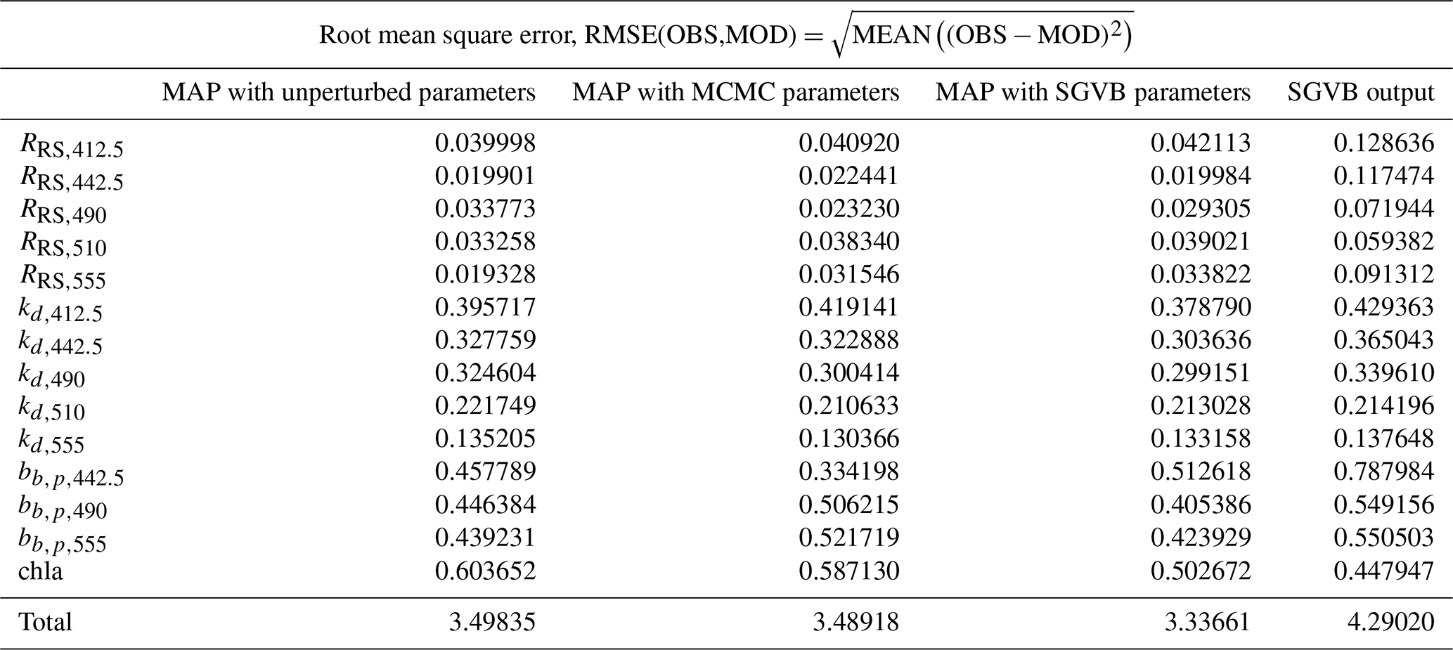
Table D2 Pearson correlation coefficient r between satellite and in situ observations and the modeled data using the maximum a posteriori (MAP) estimate with unperturbed parameters, optimized parameters with the MCMC algorithm, optimized parameters with the SGVB framework, and data modeled purely with the SGVB framework.

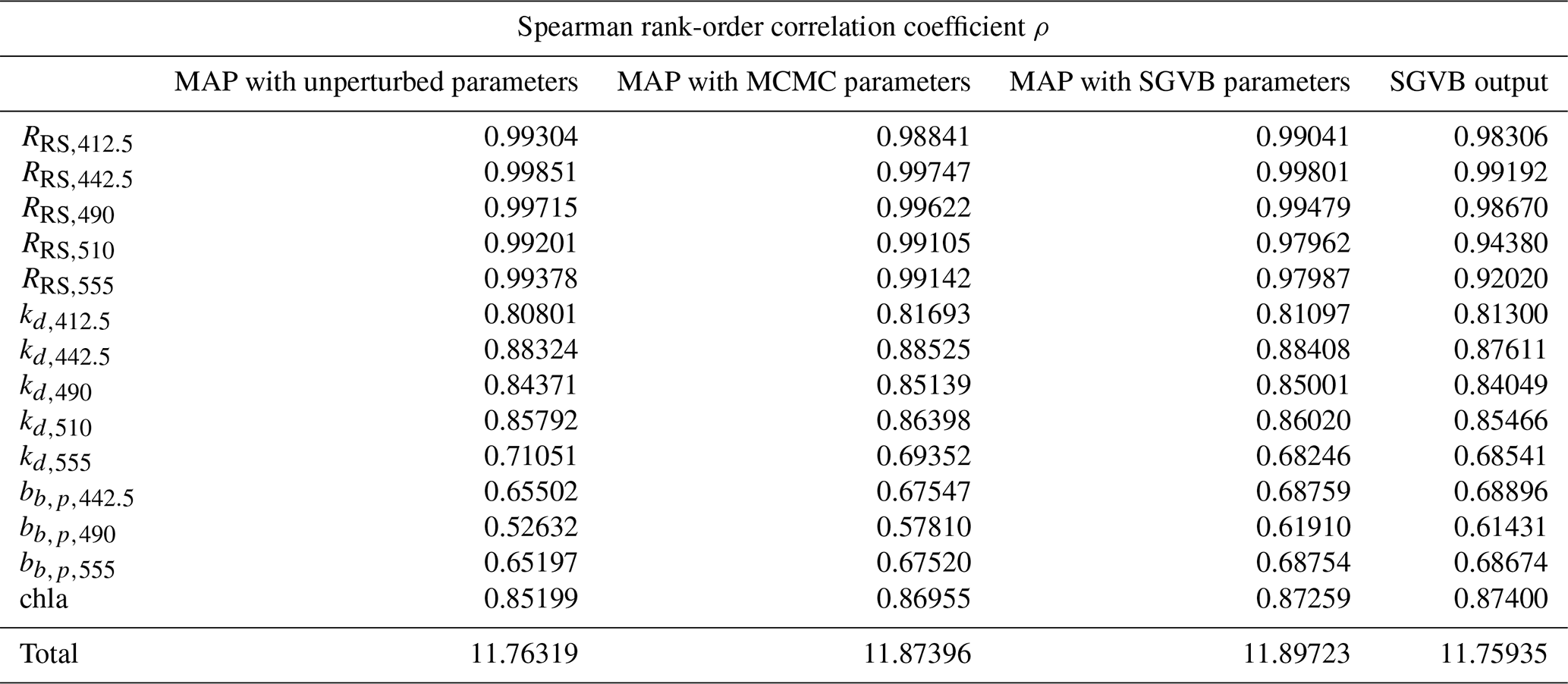
Table D3 Relative median absolute deviation (rMAD) between satellite and in situ observations and the modeled data using the maximum a posteriori (MAP) estimate with unperturbed parameters, optimized parameters with the MCMC algorithm, optimized parameters with the SGVB framework, and data modeled purely with the SGVB framework.

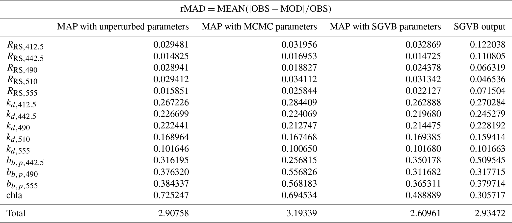
Table D4 Table of symbols used for the radiative transfer model.

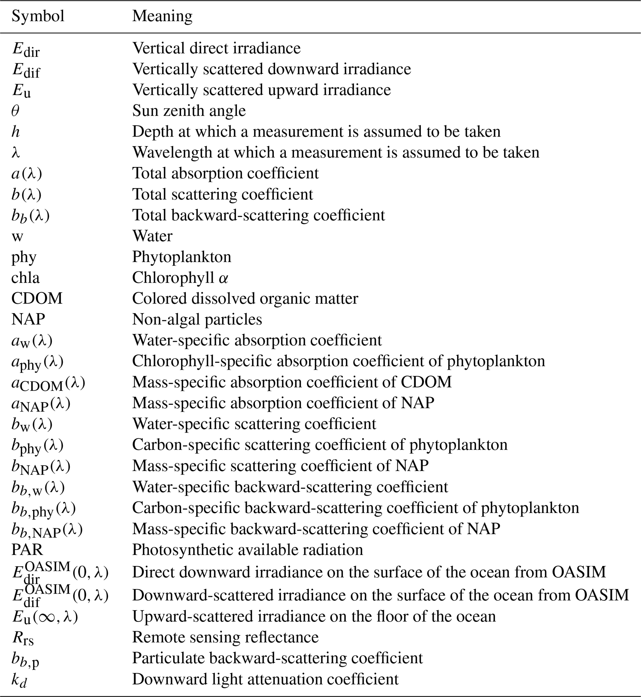
Table D5 Table of symbols and notation used for the Bayes formalism.

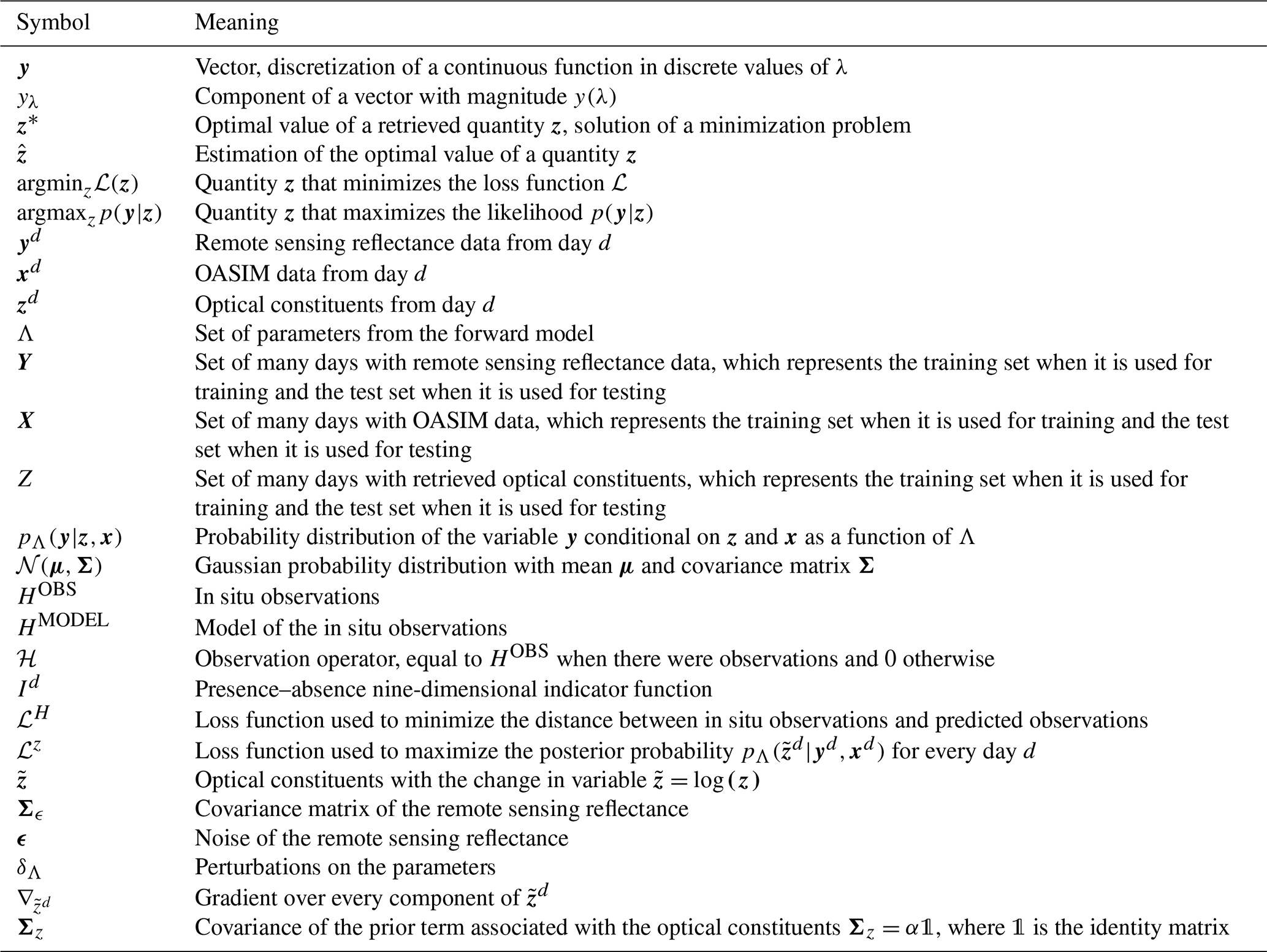
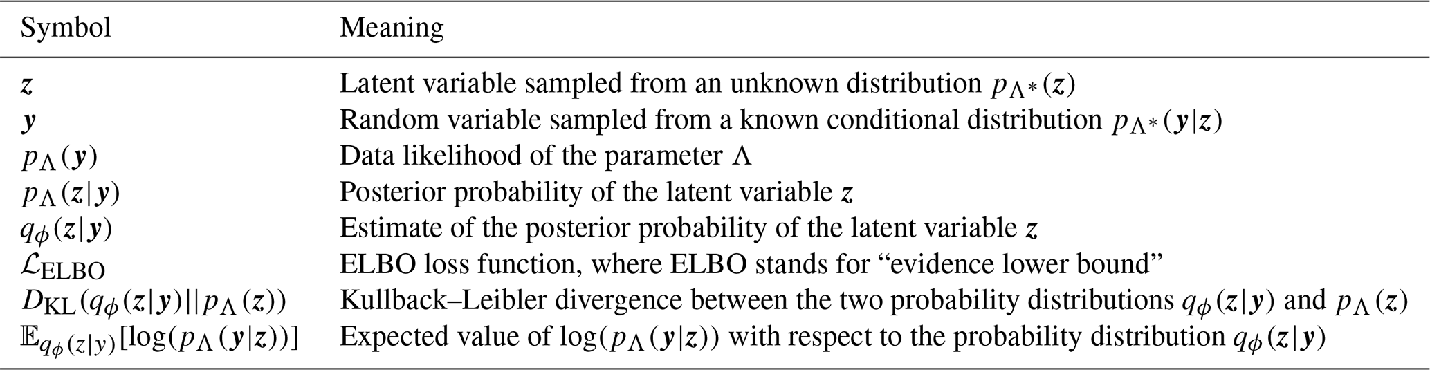
Table D6 Table of symbols and notations used for the variational Bayes formalism.