NAAC (v1.0): a seamless two-decade cross-scale simulation from the North American Atlantic Coast to tidal wetlands using the 3D unstructured-grid model SCHISM (v5.11.0)

Saltwater intrusion is an increasing concern for coastal ecosystems. While groundwater models have made progress in simulating aquifer salinization, their boundary conditions – potentially informed by ocean model simulations in shallow water systems and intertidal zones – remain constrained. Here we presented a 3D unstructured-grid model that covers the Gulf of Maine and the Mid-Atlantic Bight, and most areas of the South-Atlantic Bight along the North American Atlantic Coast (“NAAC”) for 2 decades, with a focus on the salinity simulations. This model resolves detailed geometric features of tidal tributaries down to 100 m while maintaining a resolution of 6.5 km in the coastal ocean. The two-decadal simulations from 2001 to 2020 were evaluated using a comprehensive observational dataset of elevation, temperature, and salinity. The mean absolute error in the M2 amplitude across the NOAA tidal gauges within the domain is 0.11 m. The root-mean-square deviation for salinity and temperature measurements are 0.27 PSU and 0.12 °C, respectively. The model reasonably captured the currents and circulations. For the first time, we extended a regional continental scale ocean model to the tidal wetlands to include compound flooding process. The two-decade of simulations of hydrodynamic and hydrological connectivity along the Atlantic Coast have significantly addressed numerous observational gaps in many systems. Specifically, saltwater intrusion patterns in major estuaries of the Mid-Atlantic, such as Chesapeake Bay, Delaware Bay, and other tributaries within the same hydrologic unit, exhibit significant correlations. The seamless cross-scale capability of this model facilitates future applications to land-sea interactions, such as carbon fluxes.

1 Introduction

Coastal regions are critical transition zones between saline oceanic waters and freshwater systems. Saltwater intrusion (SWI), defined as the landward encroachment of saltwater into freshwater aquifers, has become an increasing concern due to its adverse effects on drinking water quality, agriculture, and ecosystem stability (Barlow and Reichard, 2010; Werner et al., 2013). Numerical modeling, particularly groundwater models (e.g., Heiss and Michael, 2014; Paldor and Michael, 2021; Zhang et al., 2022), has been an effective tool for assessing SWI and its ecological impacts. Although oceanic forcing can be integrated into groundwater models through various approaches, such as incorporating observational data (Heiss and Michael, 2014), the spatial coverage and resolution often remain limited. Coastal ocean models can provide comprehensive boundary conditions across extended spatial and temporal scales. Larger regional models, which are typically downscaled from global ocean models, primarily emphasize deep-water regions and ocean circulation patterns (Hofmann et al., 2008; Warner et al., 2010; Lopez et al., 2020). In contrast, higher-resolution models – often with spatial resolutions of a few hundred meters – are used to capture nonlinear dynamics influenced by local geographic features, as demonstrated in studies of Chesapeake Bay (Li et al., 2005; Cai et al., 2022b), Delaware Bay (Chen et al., 2018; Liu et al., 2024), and other coastal systems worldwide (Xia et al., 2007; Xue et al., 2009, 2012; Chen et al., 2011; Li et al., 2022). However, shallow water systems and intertidal zones are often simplified or entirely excluded unless specifically targeted in certain studies (Tian et al., 2022; Cai et al., 2023). These omissions can compromise the accuracy of certain assessments, thereby limiting the effectiveness of ocean models in estimating surface water SWI or integrating with groundwater models. Moreover, these applications are often limited to specific coastal water bodies, lacking full connectivity to larger-scale oceanic forcings. Therefore, cross-scale simulations that seamlessly integrate oceanic processes with local dynamics are needed. Although recent efforts have advanced coastal resolution in global (Mathis et al., 2022; Zhang et al., 2023) and regional models (Ye et al., 2020; Cui et al., 2024) – including 10 km grids for coastal biogeochemistry (Mathis et al., 2022) and 1–2 km grids for tidal simulations (Zhang et al., 2023) – a fully integrated modeling framework that explicitly represents shallow water systems and intertidal zones in simulating salinity dynamics remains lacking.

In addition to addressing the lack of modeling tools, developing this NAAC model is also crucial for bridging observational gaps. Over the past few decades, there has been a significant accumulation of observational data, especially for key physical parameters such as water elevation, salinity, and temperature. However, these observations are unevenly distributed, with some areas heavily monitored while others lack observational coverage. For instance, Chesapeake Bay has seen extensive salinity, temperature, and nutrient monitoring since the 1980s, with numerous stations covering its main stem and tributaries, though the majority occur on a bi-weekly basis. Conversely, Delaware Bay has a few upstream stations providing daily salinity data spanning over five decades, while the remaining stations in the lower bay have records of less than 20 years or even 8 years. Beyond these two major estuaries, long-term monitoring of salinity and other parameters in smaller embayment in the mid-Atlantic region is even scarcer. Numerical model hindcasts can serve as a valuable tool to fill these observational gaps and can be further complemented by methodologies like remote sensing.

In this manuscript, we introduce a modeling system based on the SCHISM (Semi-implicit Cross-scale Hydroscience Integrated System Model) framework that covers the Gulf of Maine (GoME), the Mid-Atlantic Bight (MAB), and much of the South-Atlantic Bight (SAB) along the North American Atlantic Coast using unstructured grids. We have conducted a 20-year simulation from 2001 to 2020, focusing on tidal elevation, salinity, temperature, and velocity simulations. Our ultimate goal is to develop a reliable database to support future investigations, including SWI and other topics such as coastal carbon cycling. The study area, observational data used in this study, and model configuration are detailed in the Methods section. The following section presents model skill assessments. In the Discussion, we explore the implications for major water bodies, model uncertainties, and future directions before concluding the study.

2 Methods

2.1 Study area

The model domain covers the GoME, the MAB, and much of the SAB (Fig. 1). The GoME is a semi-enclosed body of water, bordered to the south and east by underwater banks, notably Georges Bank to the south. Along the GoME coastline are several estuaries, including the Bay of Fundy, Passamaquoddy Bay, Penobscot Bay, and Massachusetts Bay. The MAB is delineated from the GoME by Cape Cod and includes key estuaries such as Long Island Sound, Delaware Bay, and Chesapeake Bay. Long Island Sound, which stretches approximately 180 km, lies between Long Island and Connecticut. It connects to the ocean through the East River near New York City on its western end and through a narrow channel between Orient Point and Fishers Island on its eastern end. Outside of Long Island Sound, additional water bodies such as Great Peconic Bay, Little Peconic Bay, Noyack Bay, Sag Harbor Bay, Gardiners Bay, and Napeague Bay are closely linked to Long Island. Further south, Delaware Bay, a significant estuary bordered by New Jersey and Delaware, lies along the New Jersey coast. Chesapeake Bay is separated from Delaware Bay by the Delmarva Peninsula, though the two are connected via a canal. The division between the MAB and SAB occurs at Cape Hatteras, centrally located within the Albemarle-Pamlico Estuary System (APES), a complex lagoon system fed by six river basins. The coastline from Cape Fear to Cape Canaveral forms the Georgia Bight.

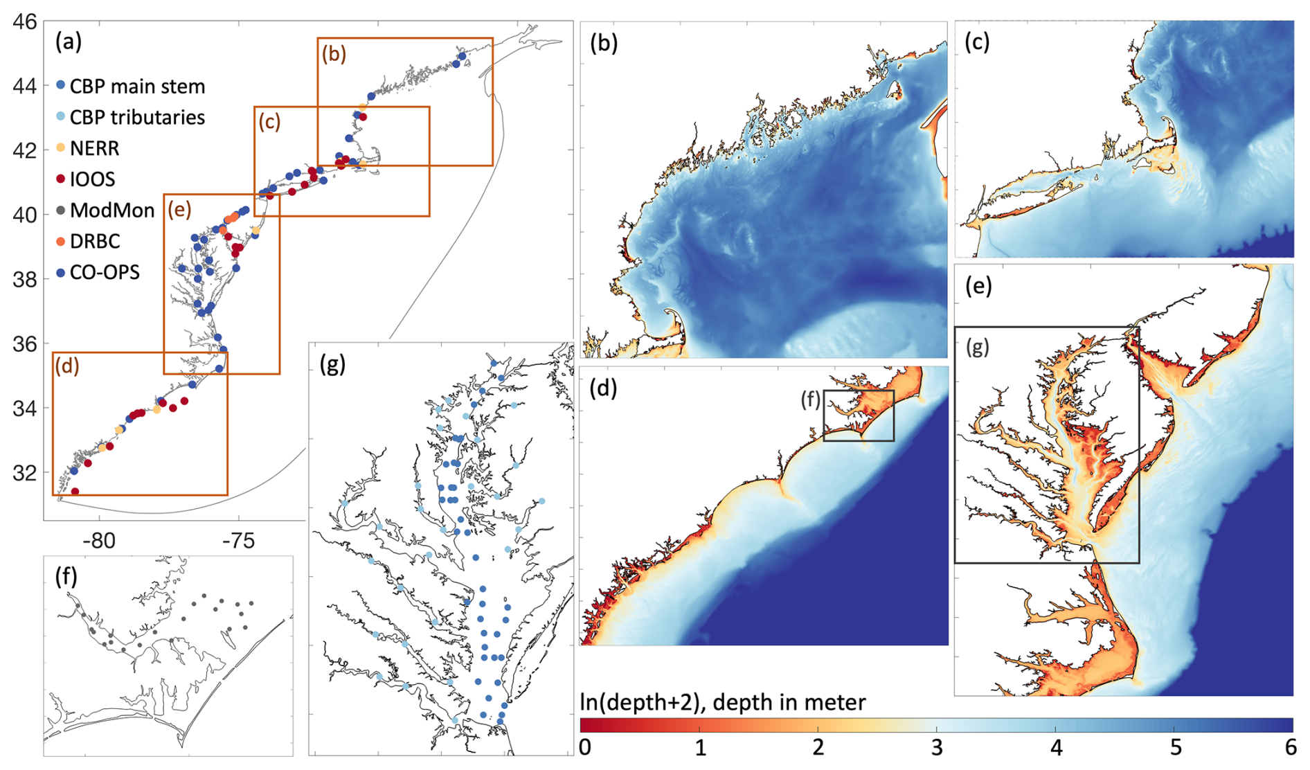
Figure 1 Study area along the North American Atlantic Coast. Scatters in (a), (f), (g) indicate the locations of monitoring stations from which data were used in this study for the skill assessments of elevation, salinity, and temperature. Panels (b)–(e) present detailed close-up views of specific areas denoted by orange boxes at (a) within the Gulf of Maine, Southern New England Coast, the South-Atlantic Bight, and the Mid-Atlantic Bight, respectively.

The GoME shoreline is predominantly rocky and scenic, shaped by glaciation (Uchupi and Bolmer, 2008). The central basin of the GoME features undersea valleys reaching depths of about 500 m, with an average depth of approximately 150 m (Uchupi and Bolmer, 2008). The MAB is characterized by a broad continental shelf extending roughly 100 km offshore (McNinch, 2004). Depths in major estuaries vary considerably: Long Island Sound has an average depth of 20 m, Delaware Bay averages 8 m, and Chesapeake Bay averages 6.5 m (Knebel et al., 1999; Dubois, 1988; Hobbs, 2004). The shoreline of Long Island Sound features a mix of sandy beaches, rocky shores, tidal flats, and tidal marshes, while the shores of Delaware Bay and Chesapeake Bay are more dominated by extensive tidal marshes (Knebel et al., 1999; Dubois, 1988; Hobbs, 2004). The SAB's geological features include “erosion remnant islands”, “marsh islands”, and “beach-ridge islands” (Zeigler, 1959). Within the APES, average depths are about 4.5 m, ranging from 7.5 m to less than 2 m (Clunies et al., 2017).

The GoME is notable for having one of the highest tidal amplitudes globally, exceeding 6 m (Ray, 2006). The GoME watershed covers an area of 180 000 km², with the Saint John and Penobscot Rivers being the largest contributors, discharging 990 and 342 m³ s⁻¹ respectively (Huntington and Billmire, 2014). On the ocean side, the Labrador Current flows along the Scotian Shelf, and subpolar North Atlantic waters mixed with eddies from the Gulf Stream enter through the Northeast Channel (Seidov et al., 2021). The overall circulation pattern in the GoME is counterclockwise, with two major outflows passing through the Great South Channel and around Georges Bank (Seidov et al., 2021). Along the MAB coast, the tidal range is generally less than 2 m (He et al., 2011). The Hudson River stream flow, along with tidal forcing, predominantly controls the stratification at the Hudson River Estuary (Ralston et al., 2008). The Delaware River is the primary tributary of Delaware Bay, contributing over 50 % of the freshwater inflow, which totals 371 m³ s⁻¹ (Kauffman et al., 2011). Tidal forcing is the main driver of circulation patterns in Delaware Bay. In Chesapeake Bay, the Susquehanna River (1135 m³ s⁻¹), followed by the Potomac River (306 m³ s⁻¹) and the James River (194 m³ s⁻¹), are the major freshwater sources, draining a watershed of 165 759 km² across six states (Ator et al., 2020). Chesapeake Bay also exhibits seasonal stratification due to its physical water characteristics (Murphy et al., 2011). In the SAB, the tidal range varies, with only 0.6 m at Cape Fear but up to 3 m along the Georgia coast (Blanton et al., 2004). The Gulf Stream flows through the Straits of Florida, follows the SAB coastline, and then veers east near the APES (Andres, 2021).

2.2 Observations

We employed an extensive observational dataset to conduct the model skill assessments (Fig. 1). For water elevation and current velocities, we primarily relied on tidal gauge and current data from the NOAA Center for Operational Oceanographic Products and Services (CO-OPS; https://tidesandcurrents.noaa.gov/products.html, last access: September 2024), metadata from the NOAA Integrated Ocean Observing System (IOOS; https://sensors.ioos.us, last access: September 2024), an hourly, 6 km surface current data from Coastal Ocean Dynamics Application Radar (CODAR) SeaSonde HF radar system at the National Centers for Environmental Information (NCEI, https://codar.com/hf-radar-technology/, last access: October 2025). Specifically for estuaries with additional long-term monitoring, we use long-term monitoring database from the Cheesecake Bay Program (CBP; http://www.chesapeakebay.net/data, last access: September 2024) for the Chesapeake Bay, high frequency measurements from the USGS and relevant products from the Delaware River Basin Commission (https://www.nj.gov/drbc/, last access: September 2024) for the Delaware Bay, and data from the Neuse River Estuary Modeling and Monitoring Project (ModMon; https://paerllab.web.unc.edu/modmon/, last access: September 2024) for the APES. Additionally, long-term monitoring data from the National Estuarine Research Reserve System (NERR; https://cdmo.baruch.sc.edu/aqs, last access: September 2024) were used to validate creek and wetland simulations.

2.3 Model configuration

For this study, we utilized the SCHISM (v5.11.0) framework, which is particularly well-suited for seamless cross-scale modeling (Zhang et al., 2025). SCHISM is distinguished by its use of mixed triangular-quadrangular unstructured horizontal grids and its flexible vertical grid coordinate system, known as Localized Sigma Coordinates with Shaved Cell (LSC2) (Zhang et al., 2015). This adaptability in both horizontal and vertical grid configurations make SCHISM especially effective in environments with complex geometrical features, such as tidal wetlands and tributaries. Additionally, SCHISM employs a semi-implicit time-stepping scheme within a hybrid finite-element and finite-volume framework to solve the Navier–Stokes equations (Zhang et al., 2016). Specifically, SCHISM utilizes an Eulerian–Lagrangian Method (ELM) for momentum advection, which further alleviates numerical stability limitations (Zhang et al., 2016). This numerical approach ensures stability and reliability, particularly under wetting and drying conditions typical of tidal wetlands (Cai et al., 2022a, 2023). Notably, the model's scheme bypasses the constraints of the Courant-Friedrichs-Lewy condition (Zhang et al., 2016), allowing for the use of relatively large time steps even with high-resolution grids that capture detailed geomorphic features. This capability significantly improves numerical efficiency and cost-effectiveness. Larger time steps can introduce temporal truncation errors, though they also reduce numerical diffusion in the ELM framework. To ensure a balance between numerical accuracy and stability, we adopted a 150 s time step that falls within validated range established through previous successful applications of SCHISM in US East Coast and global settings (Zhang et al., 2016; Ye et al., 2018, 2020; Cai et al., 2022b, 2023; Zhang et al., 2023). Overall, SCHISM stands out as one of the few hydrodynamic models ideally suited to our research purposes, which addresses the intricate interplay between land and sea, marked by complex geometrical and hydrodynamic processes.

The model's resolution varies from 6.5 km in the coastal ocean to 100 m in tidal wetlands (Cai et al., 2025a). The vertical resolution ranges from up to 63 layers in the deep ocean to a single layer in the wetlands, with an average of 23.6 layers over the entire domain. The extent of tidal marsh wetlands is based on the CONUS tidal wetland cover maps (Yang et al., 2022; Fig. 2c). Since the marsh upland migration over the simulation period is generally smaller than the resolution used in this study, we did not account for horizontal evolution in the land boundary. In a simplified version of wetland tributary and creek coverage, the model consists of 983 607 total elements and 540 895 nodes (Fig. 2b). When more details of the wetland components are included, the total element count increases to 1 075 826, and the node count rises to 592 583 (Fig. 2c). Considering the additional computational cost of incorporating tidal marsh coverage, we conducted a 20-year simulation with simplified coverage of wetlands, focusing on tributaries, and a single year (2003) with comprehensive tidal marsh coverage for sensitivity analysis.

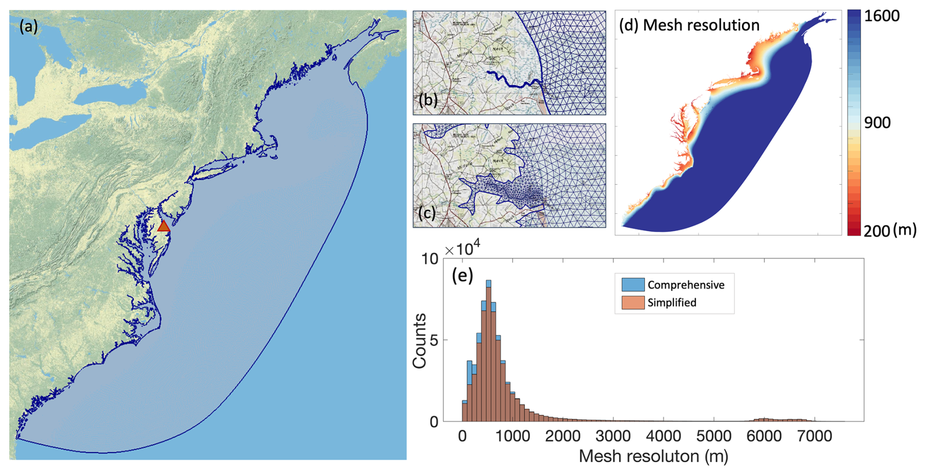
Figure 2 (a) Model domain and grid, the background is a topographic map from USGS. (b, c) Zoom-in view of the area marked by the orange triangle in (a), showing simplified and comprehensive coverage of tidal wetlands respectively. (d, e) Horizontal distribution and corresponding histogram of mesh resolutions.

We refer to NOAA Continuously Updated Digital Elevation Model (CUDEM; https://www.ncei.noaa.gov/metadata/geoportal/rest/metadata/item/gov.noaa.ngdc.mgg.dem:999919/html, last access: September 2024) and USGS Coastal National Elevation Database (CoNED; https://www.usgs.gov/coastal-changes-and-impacts/coned, last access: September 2024) for the bathymetry setup (Fig. 1b–e). To drive the model, we incorporate river discharge data from the National Water Model (NWM; https://water.noaa.gov/about/nwm, last access: September 2024) for the US East Coast (Fig. 3). For the Canadian regions, we utilize real-time hydrometric data (https://wateroffice.ec.gc.ca/map/index_e.html?type=real_time, last access: September 2024). The ocean boundary conditions are defined by the Hybrid Coordinate Ocean Model (HYCOM; https://www.hycom.org, last access: September 2024; Fig. 4); while the atmospheric forcing is provided by the North American Regional Reanalysis (NARR; https://www.ncei.noaa.gov/products/weather-climate-models/north-american-regional, last access: September 2024; Fig. 5). HYCOM data is used to initialize the model along the open ocean boundaries, while the finer, landward water bodies are initialized with reasonable constant values for each tracer (e.g., temperature and salinity). The model is then spun up for three years to establish fully developed three-dimensional initial conditions for the 20-year simulation period. This spin-up duration accounts for the range of residence times within the system, which can vary from a few days to several hundred days across different water bodies.

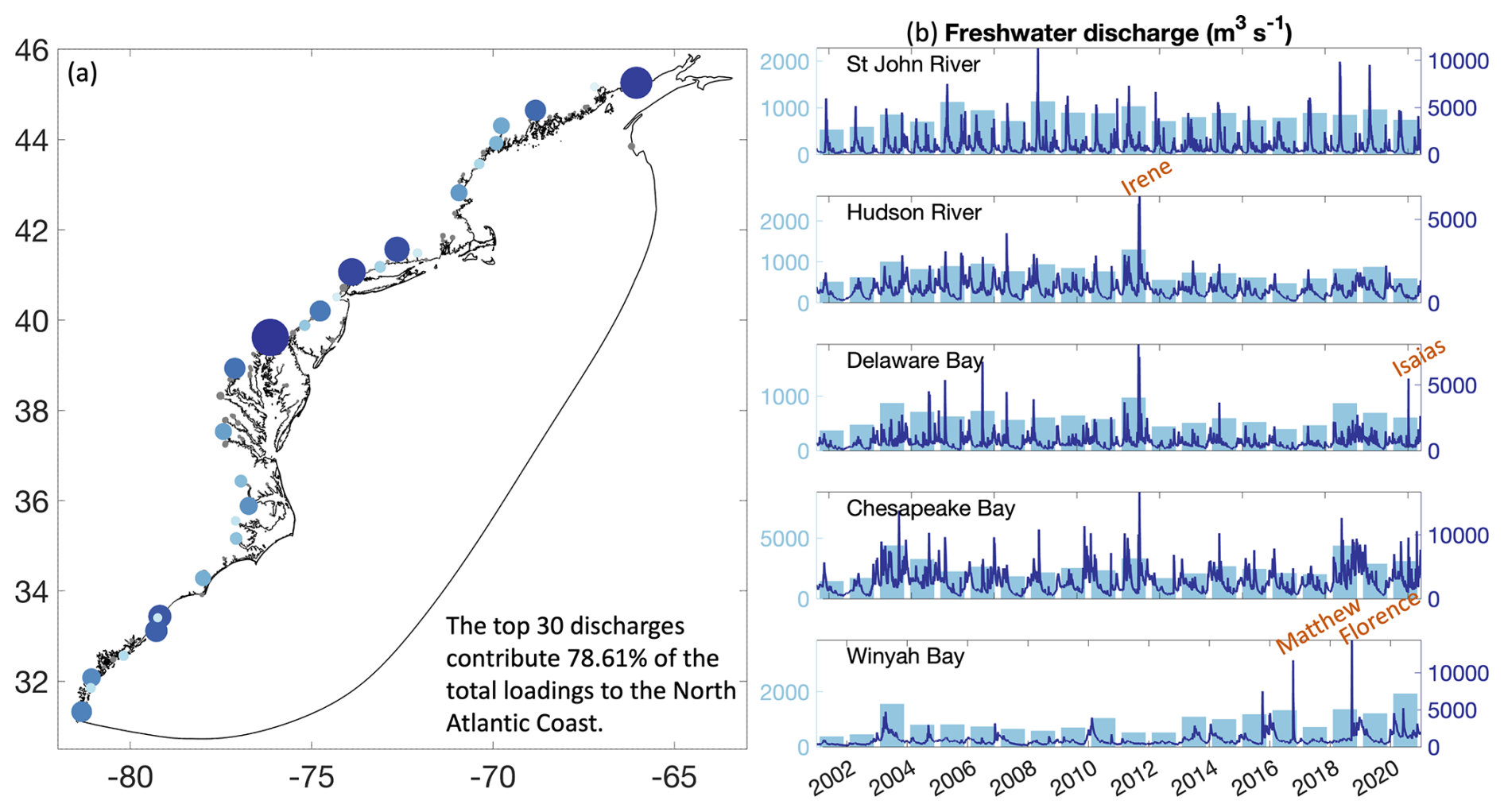
Figure 3 (a) Spatial distribution and (b) time series of freshwater discharge across the major water bodies of the North American Atlantic Coast. Darker colors, correlated to larger circle size, in panel (a) represent higher freshwater discharge amounts for the period from 2001 to 2020. Light blue bars in panel (b) represent the annual mean discharge for each of these estuaries.

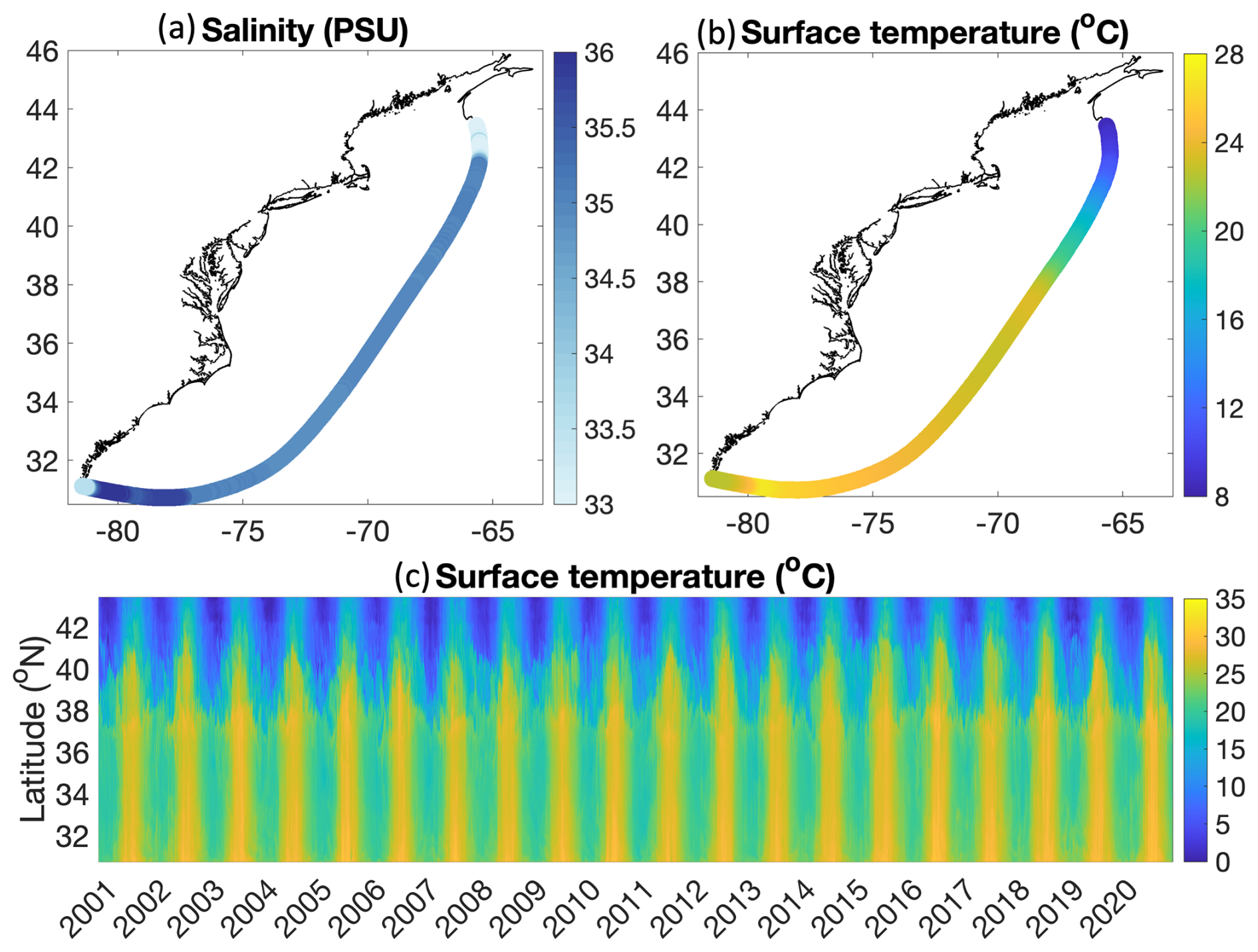
Figure 4 Ocean boundary forcing in the model. (a, b) Mean salinity and surface temperature along the ocean boundary over the 20-year simulation period. (c) Time series of surface temperature along the ocean boundary excluding the near near-shoal part on the southeastern side, from lower to higher latitudes.

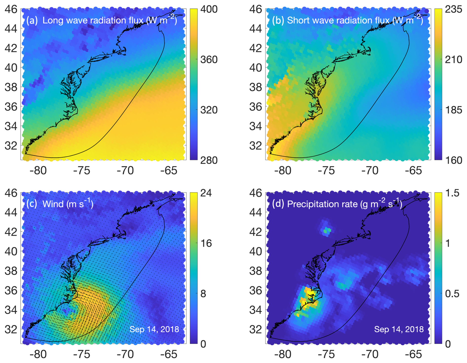
Figure 5 Atmospheric forcing in the model. (a, b) Mean downward longwave and shortwave radiation fluxes over the 20-year simulation period. (c, d) Instantaneous wind velocity and precipitation during Hurricane Florence.

3 Model skill assessments

3.1 Tidal elevations

We compare the eight tidal constituents (M2, S2, N2, K2, K1, O1, P1, Q1) between the model simulations and NOAA tidal gauge data (Fig. 6). Since the semi-diurnal M2 constituent is the dominant component along the East Coast with a higher amplitude, we specifically highlight its comparison across stations from south to north for each year (e.g., year 2003 in Fig. 6a). The mean absolute error (MAE) for the M2 constituent across all stations is 0.11 m. For the other constituents – Q1, O1, P1, K1, N2, S2, and K2 – the MAEs are 0.003, 0.015, 0.006, 0.011, 0.021, 0.022, and 0.007 m, respectively. The correlation coefficient between observations and model simulations is 0.83 for Q1, O1, P1, and K1, and 0.97 for N2, S2, and K2. Corresponding r² values are 0.87 and 0.94, respectively, indicating strong statistical significance. These performance metrics are slightly lower than reported in previous studies using SCHISM, such as Cui et al. (2024), likely due to the inclusion of shallow water stations, where uncertainties from factors like bathymetry and local friction are more pronounced. Additionally, overestimation in the GOME model tends to degrade the statistics. Despite this, the M2 amplitude remains highly consistent across most of the domain, particularly in the focused MAB study areas.

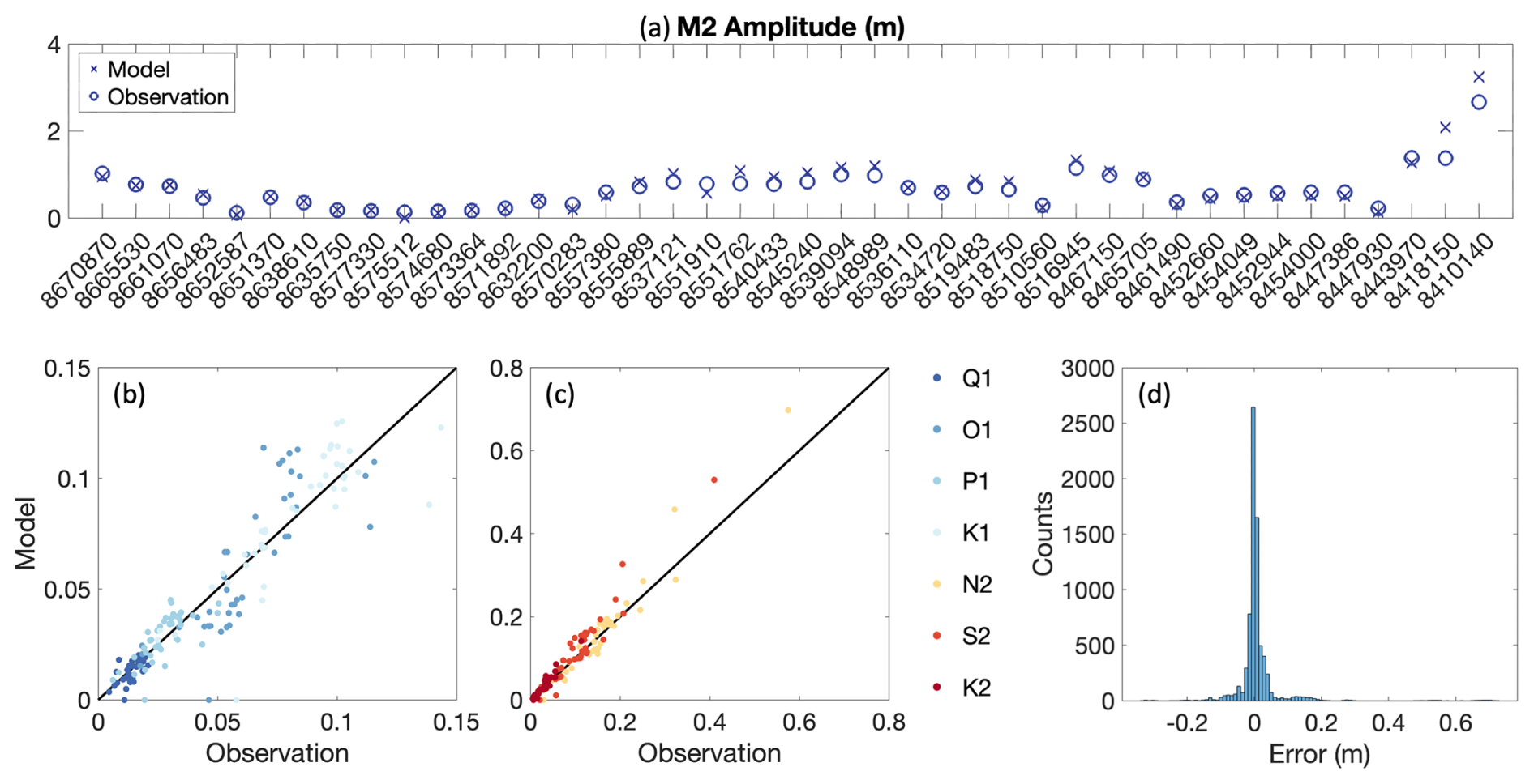
Figure 6 (a) Comparison of model-simulated and observed M2 tidal amplitude at stations along the North American Atlantic coast for year 2003. (b, c) Model versus observed values (m) for additional tidal constituents, indicated by listed colors of each contituents in the the rightside of panel (c). (d) Histogram of error differences for the eight tidal constituents across all years with available data.

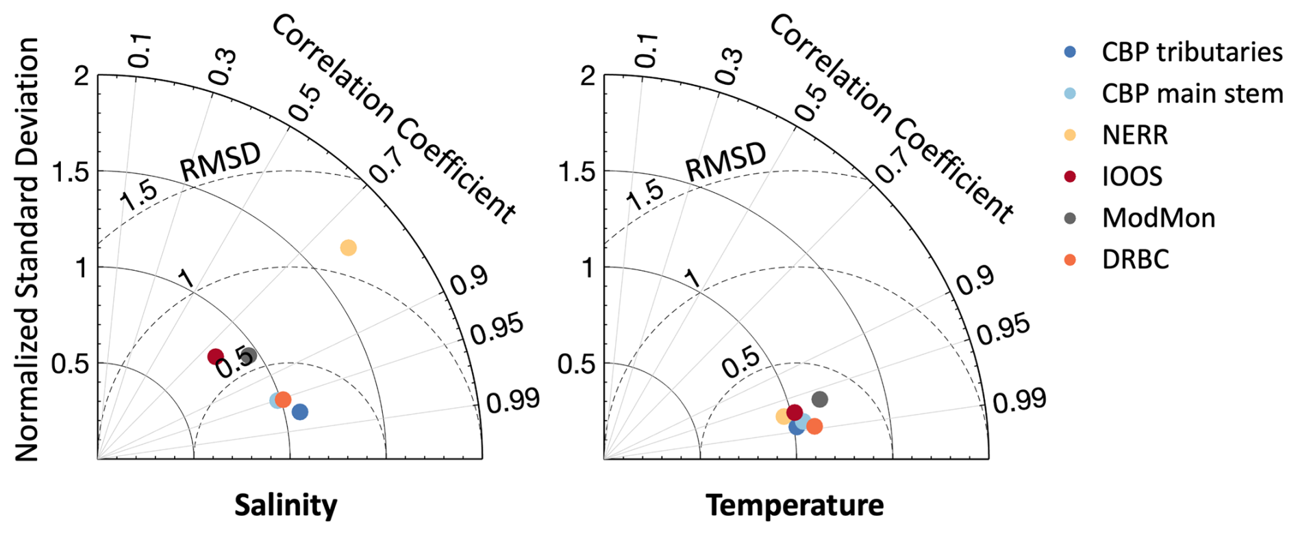
Figure 7 Taylor diagram of simulated salinity and temperature across all stations from various datasets.

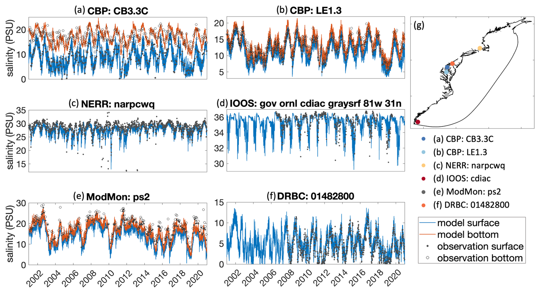
Figure 8 (a–f) Comparison of simulated and observed salinity at selected stations from the six observational data sources outlined in (g).

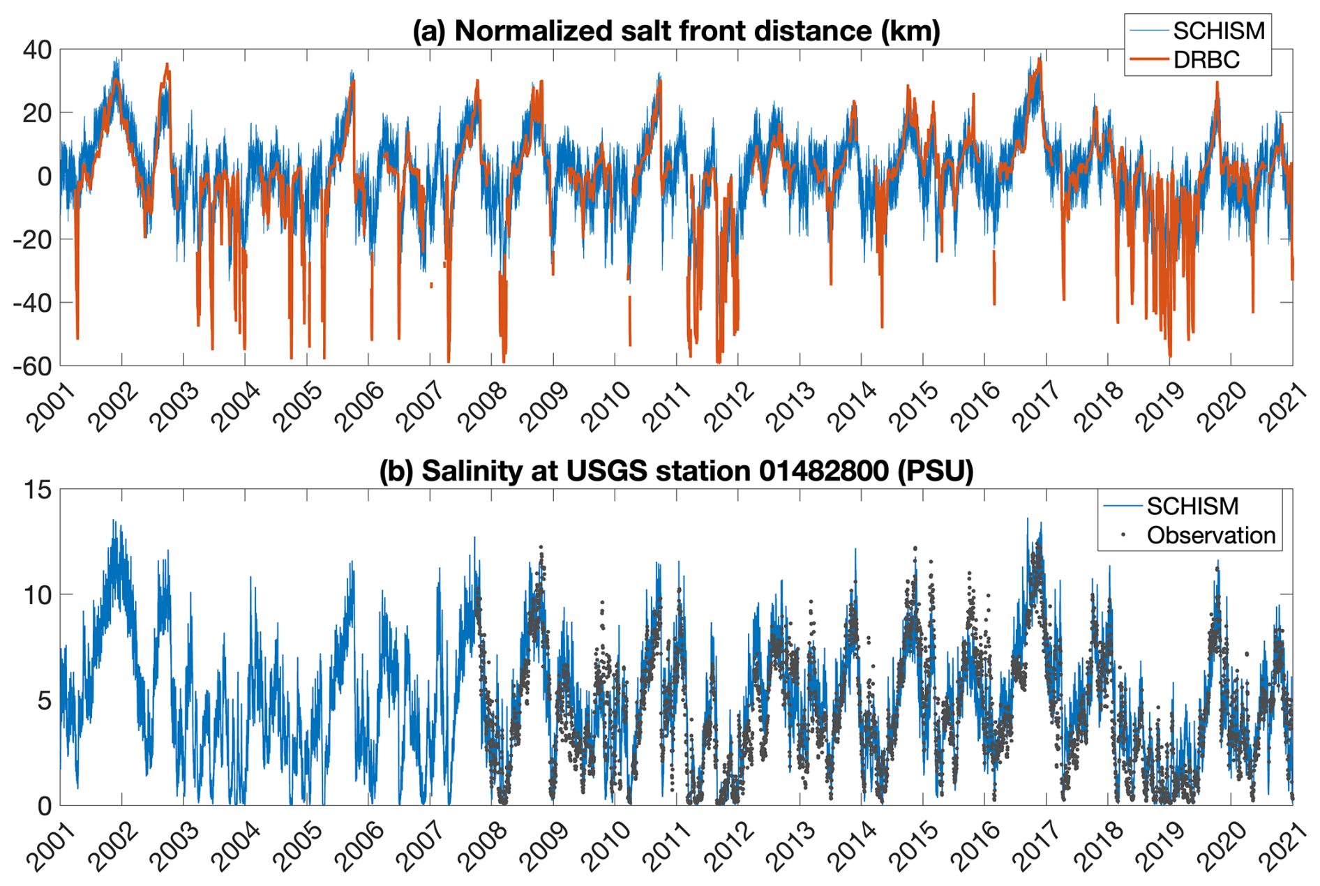
Figure 9 Validation of the simulated SWI distance in the Delaware Bay. (a) Comparison of the normalized salt front distance relative to the 20-year mean between SCHISM and DRBC. (b) Comparison of simulated salinity and observed measurements at USGS station 01482800, which represents the lower boundary for SWI estimation by DRBC.

3.2 Salinity and temperature

Available data from various sources (Fig. 1) were utilized to evaluate the model's performance in simulating salinity and temperature (Fig. 7). Both the Chesapeake Bay and Delaware Bay exhibit comparable model skills for salinity, with root mean square deviations (RMSD) less than 0.15 PSU for the main stem and 0.34 PSU for tributaries, normalized standard deviations (STD) below 1.08 PSU, and correlation coefficients (CC) larger than 0.95. Seasonal stratification, characterized by differences between surface and bottom salinity, is accurately represented in the Chesapeake Bay's main stem and major tributary channels (Fig. 8a and b). Shallow water simulations at APES, validated by ModMon, demonstrate slightly higher RMSD (0.38 PSU), a normalized STD of 0.80 PSU, and a CC of 0.82. The narrow salinity range observed at many coastal IOOS stations (e.g., 30 to 36 PSU in Fig. 8d) generally results in small RMSDs and STDs, ensuring a reasonably high CC for temporal variations. However, NERR stations show lower model performance, with an RMSD of 0.24 PSU, a normalized STD of 1.61 PSU, and a CC of 0.89. These discrepancies may be attributed to potential historical shifts in NERR station locations, introducing uncertainties in skill assessment. Additionally, the model struggles to capture high-frequency salinity fluctuations over tidal and diurnal cycles at NERR stations due to the limited resolution and absence of explicit representation of tidal marsh creeks and wetlands in the base scenario. Despite these challenges, the model reasonably captures the overall salinity magnitude and temporal variations at certain NERR stations, such as those in Narragansett Bay (Fig. 8c). Salinity simulation and modelled SWI distances in the Delaware Bay, defined as the distance from the bay mouth to the location where salinity drops below 0.5 PSU, are validated against salt front distance (similarly defined by DRBC) data from DRBC (Fig. 9). Historical DRBC data are provided as 7 d averaged daily records, which explains why SCHISM exhibits higher variability at shorter timescales (Fig. 9a). Among the salt front estimates from DRBC, the upper saltwater limit is generally more reliable than the lower limit. This is because DRBC estimates rely on interpolating distances between several monitoring stations, and the lower limit often falls beyond the monitored range, leading to noticeable underestimations of salt front distance during periods of low intrusion (Fig. 9a). SCHISM shows minimal bias in estimating the upper salt front limit, while tending to predict slightly shorter seaward salt front distances for the lower limit (Fig. 9a). To further validate this evaluation, direct comparison between salinity simulated by SCHISM and observations from a USGS station – used as one of DRBC's reference points for salt front distance – shows strong agreement (Fig. 9b).

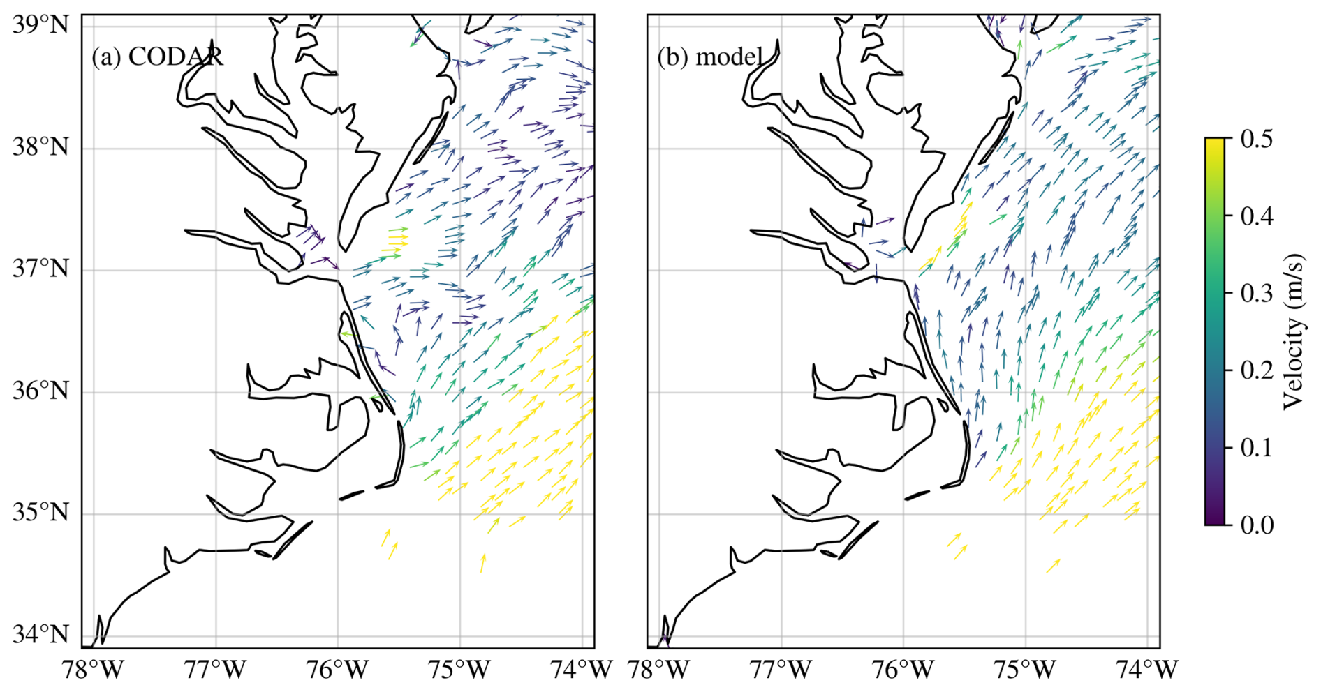
Figure 10 Daily averaged currents over Mid-Atlantic coast from (a) CODAR and (b) model on 30 July 2015.

The temperature time series in estuaries and coastal regions show RMSD values below 0.13 °C across all areas, with normalized STD ranging from 0.94 to 1.15 °C and CC exceeding 0.96 (Fig. 7). The largest spatial errors are mainly concentrated in shallow tributaries, likely due to known overestimations of shortwave/longwave radiation and air temperature in NARR. We plan to explore alternative atmospheric forcing products (e.g., ERA1) in future versions of NAAC to address this issue. In addition to the station-based time series, we evaluated large-scale sea surface temperature by comparing model simulations with the NOAA OI SST reanalysis dataset (Fig. S5; https://psl.noaa.gov/data/gridded/data.noaa.oisst.v2.highres.html, last access: August 2025). The comparison yielded an overall MAE of 0.55 °C and a RMSD of 1.09 °C across the overlapping ocean domain, demonstrating the model's ability to capture basin-scale features such as the Gulf Stream. This representation is further supported by current simulations, which show a RMSD of 0.24 m s⁻¹ for magnitude and 90.63° for direction when compared with observations across the region (Fig. 10). Although the overall RMSD for current directions across the region is relatively large, the directional RMSD at locations with velocities exceeding 1 m s⁻¹ is only 10.69°. However, the model domain does not fully encompass the entire Gulf Stream pathway, making the simulation highly dependent on the boundary conditions provided (Fig. 4).

3.3 Current velocities

In large coastal ocean areas, daily-averaged surface currents are compared with observations from CODAR (e.g., MAB at Fig. 10). Overall, the model reproduces the surface circulation but slightly underestimates the velocity magnitude near APES. Given the fact that no data assimilation was used, the model skill for the surface currents is generally acceptable. We take available time series data from NOAA gauges over Chesapeake Bay, Delaware Bay, and New York Bay for the validation of current simulations (Fig. 11). At New York Bay, the model tends to have slight phase shift but comparable magnitude and temporal patterns. The model slightly overestimated or underestimated certain peak velocities at both lower Chesapeake Bay and Delaware Bay. These bias patterns are largely station-specific rather than temporally correlated. At Delaware Bay, the overestimation is more prominent during ebb/flooding tides, whereas at New York Bay, the model shows underestimation during similar periods. This station-dependent bias likely reflects local bathymetric complexities or grid resolution limitations, which we plan to improve as needed in future model updates.

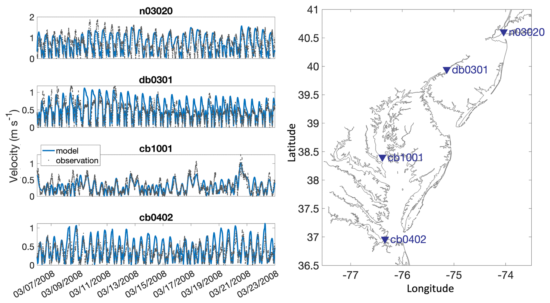
Figure 11 Time series comparison of model-simulated and observed current velocity at stations across the major estuaries along the Mid-Atlantic coast.

4 Discussion

4.1 Applications in major waterbodies along the North American Atlantic Coast

While numerous observations have been made over the centuries, significant gaps remain in many systems. The development of this model offers a valuable database for addressing these deficiencies. In cases with limited temporal and spatial coverage, it is crucial to validate the model using available data while bridging these gaps to support future research in coastal studies. For scenarios requiring higher resolution to capture finer details of localized processes, this model provides a solid foundation, potentially serving as an initial condition or offering boundary forcings. Additionally, the following sections present sample applications related to SWI and tidal fluxes in typical mid-Atlantic waterbodies. However, this manuscript does not delve deeply into these specific topics. Instead, it aims to demonstrate examples and explore the potential future applications of the developed model.

4.1.1 Estimation on saltwater intrusion and salt front distances

Salinity observations are significantly less abundant compared to measurements of temperature or water levels. For instance, the NOAA CO-OPS database contains over two decades and up to one century of water level data from more than 50 stations along the East Coast, yet only a few stations provide salinity measurements, and these are for much shorter durations. While the relatively small variability of salinity in ocean waters may explain its lower priority in NOAA's observational efforts, salinity data from USGS stations are also more limited compared to the measurements of discharge. Consequently, the availability of salinity simulations from this model, particularly in oligohaline, mesohaline, and polyhaline zones, offers valuable support for scientific research and management practices.

One use of this model is to serve as an important supplement for the monitoring and prediction of SWI in the Delaware Bay and the surrounding Delmarva region, which has been identified as highly vulnerable to SWI over recent decades (Mondal et al., 2023). An accurate validation to the upper stream USGS stations supports a reasonable capture of the salt front distance as supported by the salt front estimation data provided from DRBC (Fig. 9). Notably, SCHISM can not only bridge the temporal gaps of observation but also correct the salt front locations when the intrusion has not reached the first USGS station, under which conditions the estimated salt front distance from DRBC may tend to be underestimated by interpolation constraints due to relatively few observational stations. Importantly, we found the salt front distance at the Delaware Bay and Chesapeake Bay show significant correlation with r-square larger than 0.64 (Fig. 12). Given that the salt front distance is largely driven by the freshwater discharge in estuaries (Ross et al., 2015), and these two water bodies, along with other tributaries, share a drainage source from the same second level hydrological unit, this significant correlation is understandable.

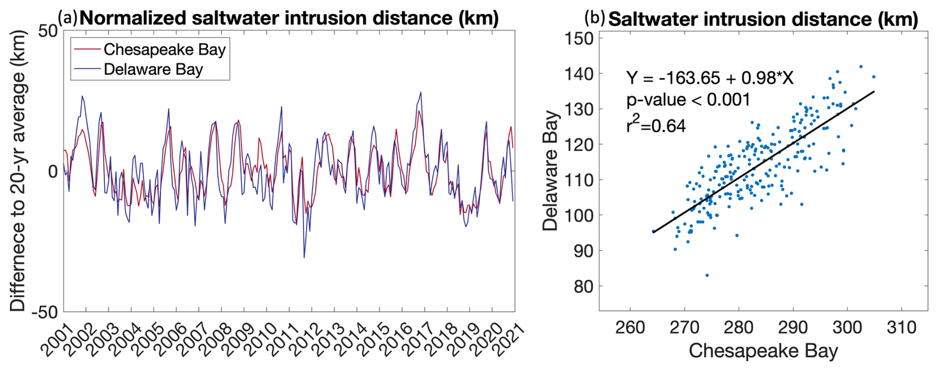
Figure 12 Simulated saltwater intrusion distance in the Chesapeake and Delaware Bays, presented as (a) a normalized view and (b) correlation analysis.

4.1.2 Water exchange between major estuaries and the coastal Atlantic

Tidal flushing plays a key role in exchanging water between coastal and estuarine zones, offering essential insights for studies on processes like coastal carbon cycling (Sanford et al., 1992; Najjar et al., 2018). However, observations are not always available on large spatial and temporal scales. Here we are showing an example of modeled tidal flow fluxes at the gate or major inlets of the three significant waterbodies at mid-Atlantic – Delaware Bay, Chesapeake Bay, and the APES (Fig. 13). While the net fluxes are always associated with the riverine discharge as denoted in Fig. 3, the flood and ebb tidal fluxes have distinct patterns among these three systems. Spring–neap tidal signals are most apparent at the Delaware Bay mouth due to its larger tidal range, producing tidal fluxes roughly twice those of Chesapeake Bay and 16 times those of Hatteras Inlet. The relatively smaller river discharge into Delaware Bay further reduces the influence of riverine and wind-driven variability, allowing tidal signals to dominate (Fig. 6a).

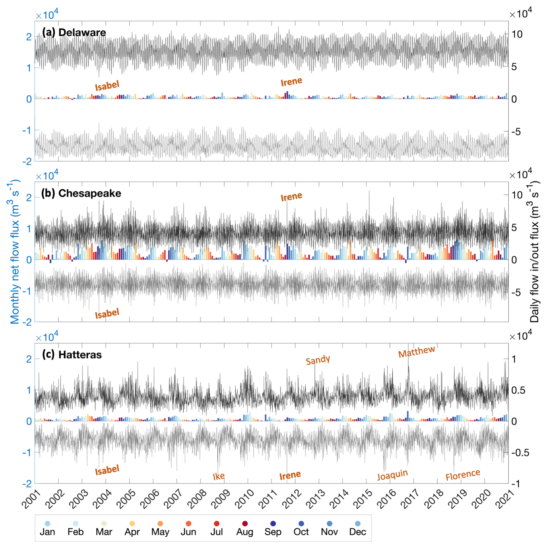
Figure 13 Tidal fluxes across the mouths of (a) Delaware Bay, (b) Chesapeake Bay, and (c) Hatteras Inlet at APES. Colored bars represent monthly net flow, while black and grey lines show daily inflow and outflow. Notable hurricanes are marked along the timeline at the affected locations, with bold text indicating those that impacted multiple sites. Except for the right-hand vertical axis in panel (c), all left-hand vertical axes share the same scale. The right-hand vertical axes in panels (a) and (b) also share the same scale.

The disturbances caused by numerous hurricanes are clearly noticeable at the Hatteras Inlet, while at Delaware Bay, also these disturbances are still visible but dwarfed by the generally large tidal range (Fig. 13a and c). However, we could still notice occasions such as Hurricane Irene in 2012 lead to an abnormal high-net flow in September compared to other periods in those two decades (Fig. 13). The in/out fluxes at Hatteras show relatively less structures from tide than the other two bays; instead, wind forcings might be dominant at this low-tidal range (e.g., <0.8 m) location (Fig. 13). In summary, the hurricane disturbance can be seen in flux directions, depending on the wind directions, track, and precipitation conditions.

4.2 Resolving tidal wetlands and their connectivity to shelf-scale processes

In this model development practice, we conducted a one-year simulation of an entire coverage of wetlands for a sensitivity test on this regional-scale model. The model results show that including tidal wetlands has minor impacts on the model skills in the physical variables away from the wetlands. In certain areas, especially for regions with complex geometry of tidal creeks and tidal marshes, such as near some of the NERR stations, including the wetland helps local simulations (Fig. 14). However, given the relatively small widths of the tidal creeks, an effective incorporation of a comprehensive wetland details will significantly increase the model grid size and therefore computational costs (Cai et al., 2023). To explicitly include the impacts of the wetlands on coastal processes, the model resolution at these areas needs to decrease to at least 50 m and even be less than 10 m for some essential creeks. In addition, the local bathymetry of the creeks needs to be fully resolved, and the varying drag force from the vegetation at the marsh platform from at the non-vegetated creeks need to be distinguished (Cai et al., 2022a). For the future directions, improvement in bathymetry from sources with an even more realistic Digital Elevation Model (DEM) could be very helpful in the simulations. We could further incorporate other ocean boundary and atmospheric forcing sources in further evaluation. Furthermore, a two-way coupling of ocean model and regional-scale coastal groundwater could be considered to incorporating the roles of submarine groundwater discharge on the costal processes.

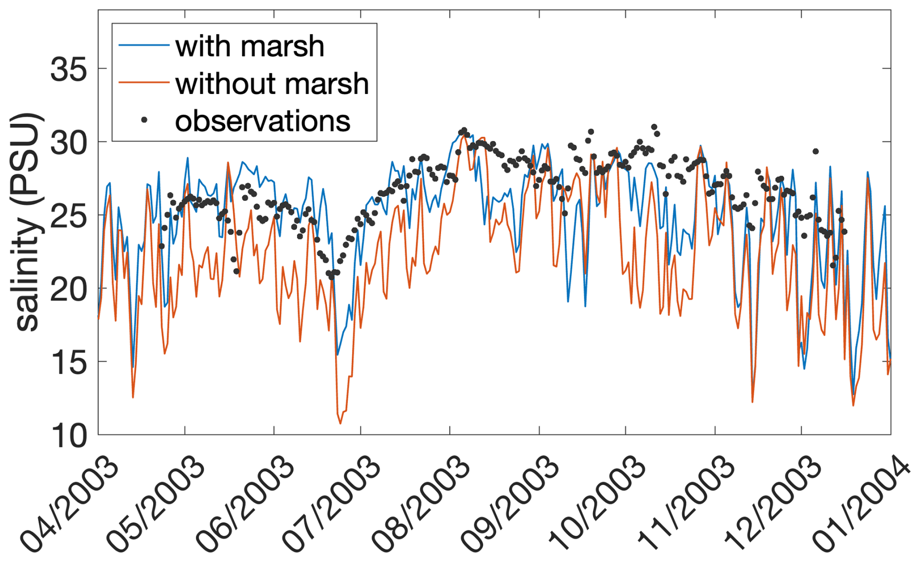
Figure 14 Salinity simulations with and without extended tidal wetland coverage versus observed data at the NEER station (jacb9wq).

To investigate the connectivity between tidal wetlands and the shelf, we conducted an idealized one-year numerical experiment in which a passive conservative tracer was continuously released from the Plum Island Estuary (PIE) – the largest tidal marsh system along the New England coast. The resulting tracer distributions (Fig. 15) reveal progressive offshore and along-shelf transport of marsh-sourced material over time. Initially concentrated near the estuary, the tracer gradually spreads southward and offshore, with significant accumulation along the southern Maine coast and within semi-enclosed shelf regions such as Georges Bank, Southern New England Shelf, and the Mid-Atlantic Bight. This evolving pattern underscores the dominant role of large-scale shelf processes – including the cyclonic Georges Bank Gyre, the northeastward Gulf Stream along the shelf break, and the southwestward Shelfbreak Jet near the inner shelf – in shaping cross-shelf exchange and material retention. While this idealized tracer experiment cannot be directly validated due to the absence of long-term tracer observations sourced from coastal wetlands, the modeled pathways align qualitatively with known circulation structures and transport trends from prior regional studies. The simulation serves as a useful exploratory tool for illustrating how signals from coastal wetlands can be redistributed over broad spatial scales by shelf dynamics, reinforcing the importance of capturing these interactions in cross-scale modeling frameworks.

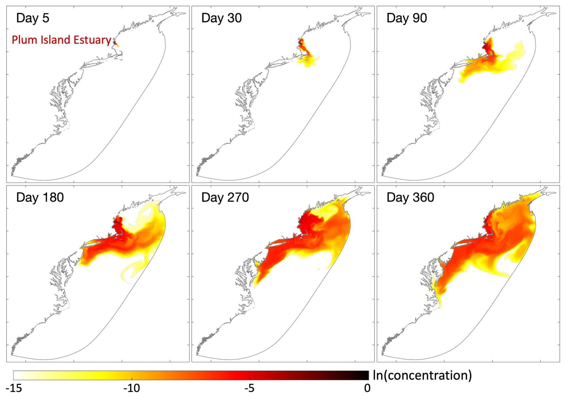
Figure 15 Log-scale plot showing the distribution of a passive tracer released continuously from a constant source of wetlands at Plum Island Estuary.

5 Conclusions

In this study, we developed a 3D unstructured-grid model NAAC for the North American Atlantic Coast, encompassing the GoME, the MAB, and much of the SAB. This model, based on the SCHISM (v5.11.0) framework, provides a seamless cross-scale simulation extending from the coastal ocean to tidal wetlands, allowing for the representation of fine-scale hydrodynamic and salinity dynamics over a two-decade period (2001–2020). Through extensive validation against observational datasets, the model demonstrated strong performance in simulating key physical variables such as tidal elevation, salinity, and temperature. One of the key contributions of this work is the integration of shallow water systems and intertidal zones within a regional-scale model, addressing long-standing gaps in hydrodynamic connectivity along the Atlantic Coast. Our results highlight significant correlations in saltwater intrusion patterns between major estuaries, suggesting common hydrological drivers at a broader scale. The model also captures the complex tidal exchange processes that govern estuarine circulation, making it a valuable tool for future studies on coastal carbon cycling, biogeochemical transport, and climate-driven changes in coastal hydrodynamics. Overall, NAAC represents a significant step forward in coastal ocean modeling, offering a foundation for future applications in coastal hydrodynamics, ecosystem studies, and climate resilience planning. The availability of this dataset will support interdisciplinary research and inform management strategies aimed at mitigating the impacts of saltwater intrusion and sea-level rise on coastal ecosystems.