A component-based modular treatment of the soil–plant–atmosphere continuum: the GEOSPACE framework (v.1.2.9)

The soil–plant–atmosphere continuum (SPAC) system is a complex and interconnected network of physical phenomena, encompassing heat transfer, evapotranspiration, precipitation, water absorption, soil water flow, substance transport, and gas exchange. These processes govern the exchange of energy and water within the SPAC system. Modeling the SPAC system involves multiple disciplines, including hydrology, ecology, and computational science, making a physically based approach inherently interdisciplinary for capturing the complexity of the system.

The present study introduces the Soil–Plant–Atmosphere Continuum Estimator in GEOframe (GEOSPACE), a new ecohydrological modeling framework, in particular its one-dimensional development, GEOSPACE-1D. GEOSPACE leverages and extends selected components from the GEOframe modeling system, while also integrating newly developed modules, to comprehensively simulate water transport dynamics in the SPAC system. The framework of GEOSPACE-1D is a tool designed to facilitate robust, reliable, and transparent simulations of SPAC interactions. It embraces the principles of open-source software and modular design, aiming to promote open, reusable, and reproducible research practices. Instead of relying on a single monolithic model, we propose a component-based modeling approach, where each component addresses a specific aspect of the system. Object-oriented programming (OOP) is adopted as the foundational framework for this approach, providing flexibility and adaptability to accommodate the ever-changing nature of the SPAC system. This compartmentalization serves two critical purposes: validating individual processes against analytical solutions and facilitating the integration of novel processes into the system.

The paper emphasizes the significance of modeling the coupling between infiltration and evapotranspiration through two “virtual” simulations based on real-world input data from the “Spike II” experiment to explore the interplay between plant transpiration, soil evaporation, and soil moisture dynamics, highlighting the need to account for these interactions in SPAC models. Overall, GEOSPACE-1D represents an approach to SPAC modeling providing a flexible and extensible framework for studying complex interactions within the Earth's critical zone. It is worth recalling that the fundamental premise of GEOSPACE-1D is not to create a single soil–plant–atmosphere model but to establish a system that allows the creation of a series of soil–plant–atmosphere models adapted to the specific needs of the user's case study.

1 Introduction

The soil–plant–atmosphere continuum (SPAC) encompasses a wide range of interconnected physical phenomena, including heat transfer, evapotranspiration, precipitation, water absorption and infiltration, soil water flow, substance transport, and gas exchange, all of which influence the exchange of energy, matter, and water among these three compartments (Fisher and Koven, 2020; Blyth et al., 2021; Li et al., 2021). A variety of formulations for the underlying physics of these processes are currently debated, including soil–root interactions (Steudle, 2000; Schröder et al., 2008; Manoli et al., 2017), alternative formulations for plant hydraulics (Verhoef and Egea, 2014b; Silva et al., 2022; Giraud et al., 2023), constraints imposed by water-limited availability (water stress) and their combinations (Lhomme, 2001; Verhoef and Egea, 2014b), the characterization of soil properties in the presence of roots (York et al., 2016; Carminati and Javaux, 2020), and coupling plant behavior with atmospheric transport (Katul et al., 2001; Poggi et al., 2004; Mauder et al., 2020; Finnigan et al., 2009). Additional discussions include the statistical description of plant canopies (Kerches Braghiere, 2018; McGrath et al., 2016), individual plant traits (Mencuccini et al., 2019; Cranko Page et al., 2024), and the interactions between trees, soil microbiology (Cassiani et al., 2015; Simard et al., 1997), and atmospheric processes (Brunet, 2020). Depending on specific objectives and the temporal and spatial scales of analysis, various simplifications of these processes are often employed (Anderson et al., 2003; Donovan and Sperry, 2000).

Given the complexity of the SPAC domain, numerous modeling approaches have been developed. These include physically based models (PBMs) (Fatichi et al., 2016) and those leveraging statistical learning techniques, such as machine learning (ML) (Pal and Sharma, 2021). Traditional PBM-based land surface models, widely used in hydrology and agronomy, often employ simplified governing equations, such as the Penman–Monteith equation (Pereira et al., 2015) or the Priestley–Taylor approach (Formetta et al., 2014). More advanced types of SPAC models include SVAT (soil–vegetation–atmosphere transfer) models and LSMs (land surface models). While SVAT models focus on vegetation-related processes and LSMs cover a broader range of processes, the distinction between these categories is not always clear-cut (Blyth et al., 2021; Fisher and Koven, 2020; Pal and Sharma, 2021). For a comprehensive model overview, we recommend Blyth et al. (2021) for LSM comparisons, Fatichi et al. (2016) for process-based model capabilities, and Bonan et al. (2024) for Earth system modeling perspectives. Additional valuable references offering complementary perspectives include Overgaard et al. (2006), McDermid et al. (2017), Vereecken et al. (2019), Bierkens (2015), and Miralles et al. (2025). These references collectively indicate that achieving a deeper understanding and accurate modeling of SPAC interactions requires highly interdisciplinary approaches which, in our assessment, necessitates moving beyond the traditional notion of “model”.

To address the implementation challenges arising from the complexity of SPAC processes and the diversity of possible solutions, the literature advocates dividing software into self-contained, independent components interconnected through a supporting software layer. This approach, known as “modeling by components” (MBC), has been in use for over 40 years (Holling, 1978) and was initially developed to integrate knowledge across disciplines (Moore and Hughes, 2017). In recent decades, MBC has gained significant importance within environmental modeling (Argent, 2004; Serafin, 2019). Notable MBC implementations in hydrology and meteorology include frameworks as TIME (Rahman et al., 2003), CSDMS (Peckham et al., 2013), ESMF (Collins et al., 2005), OMS (David et al., 2013), and RAVEN (Craig et al., 2020). A more extensive list can be found in Chen et al. (2020).

True MBC systems adopt a service-oriented architecture (SOA) (Richards and Ford, 2020), which facilitates the integration of heterogeneous data sources. SOA frameworks are inherently scalable, designed to operate across diverse machines and architectures, and are fundamental to the infrastructure of the digital Earth (Rigon et al., 2022; David et al., 2013). By abstracting computational details, SOA enables users to focus on modeling rather than the complexities of the underlying computational engines. Despite the advantages of MBC concepts, practical implementation remains challenging. It often requires programmers to adopt new workflows and habits. The OMS framework has explicitly addressed these challenges, bridging the gap between conceptual elegance and practical usability (Lloyd et al., 2011). These frameworks aim to meet broader scientific needs while adhering to good scientific practices, as outlined in Rigon et al. (2022).

To our knowledge, no existing SVAT models or LSMs implement a true MBC structure, although some exhibit highly modular software organization. Beyond leveraging MBC, incorporating internal modularity through object-oriented programming (OOP) principles is equally important, as emphasized by Rouson et al. (2011) and Gardner and Manduchi (2007). OOP promotes code reuse, improves readability, and enhances efficiency and scalability. Moreover, employing appropriate levels of abstraction, as theorized by Berti (2000), enhances model adaptability and reliability while minimizing the need for modifications to existing code.

These principles, which we have found inadequately implemented in previous modeling efforts, have guided the development of a new ecohydrological modeling framework within GEOframe, GEOSPACE, the Soil–Plant–Atmosphere Continuum Estimator in GEOframe, which we present in this paper. This software platform integrates MBC concepts with OOP principles to transcend traditional modeling paradigms, focusing on the interactions and feedback mechanisms within the SPAC. The MBC approach maintains complete control over code evolution while creating a unified framework applicable to ecohydrological, agrometeorological, and hydroclimatological communities. In developing GEOSPACE, we have prioritized strict adherence to FAIR principles (findable, accessible, interoperable, and reusable) (Wilkinson et al., 2016) to ensure openness and availability. Additionally, we address specific algorithmic limitations identified in similar software, particularly regarding inadequate treatment of transitions between saturated and unsaturated conditions and the implementation of appropriate numerical solvers. The GEOSPACE framework functions as an integral component of the GEOframe system, and it uses some of the components available in GEOframe to simulate the water transport in the continuum SPAC, thus being the ecohydrological model of GEOframe. GEOframe is an open-source, component-based hydrological modeling system (Formetta et al., 2014; Bancheri et al., 2020). Rather than being a single model, GEOframe is a modular framework, where each part of the hydrological cycle is implemented in a self-contained building block, an OMS3 component (David et al., 2013). Models available in GEOframe cover a wide range of processes, including geomorphic and DEM analysis, spatial interpolation of meteorological variables, radiation budget estimation, infiltration, evapotranspiration, runoff generation, channel routing, travel time analysis, and model calibration. It allows users to build custom modeling solutions to address various hydrological challenges. The GEOSPACE framework presented here was developed by composing and extending existing GEOframe components, WHETGEO (Water Heat and Transport) (Tubini and Rigon, 2022), GEOET (EvapoTranspiration), and BrokerGEO, to simulate complex soil–vegetation–atmosphere interactions in the critical zone. While GEOSPACE builds upon existing components in GEOframe, this work contributes three main innovations: (i) the development of GEOET, a new evapotranspiration module evolved from the established ETP-GEOframe component (Bottazzi, 2020); (ii) the implementation of BrokerGEO, a new coupler component enabling the dynamic interaction between evapotranspiration and infiltration processes; and (iii) the extension of WHETGEO (Tubini and Rigon, 2022) to allow modular and seamless coupling with GEOET and BrokerGEO. These contributions represent both algorithmic and structural advances over previous models, such as the monolithic GEOtop framework (Rigon et al., 2006), and establish GEOSPACE as the ecohydrological core of GEOframe.

This paper is organized as follows: Sect. 2 provides an overview of the GEOSPACE system and its hierarchical software architecture. Sections 3, 4, and 6 introduce its main components: WHETGEO, GEOET, and BrokerGEO. Section 5 discusses the implementation of the stress function, addressing evapotranspiration constraints caused by water scarcity or other environmental factors. Each section follows a similar structure and includes a concise overview of the mathematical equations employed and relevant software implementation details. Readers less interested in the informatics can skip the latter portions of these sections. Section 7 presents two “virtual” simulations based on real input data to showcase the potential applications and capabilities of the coupled system of GEOSPACE-1D and verify its correct functioning. In addition, a dedicated subsection describes general model inputs and outputs in detail. Finally, Sect. 8 describes the availability of the code, executables, training materials, and fair use conditions and concludes the paper.

While this paper does not delve into the rationale behind the implemented physics, which is addressed in other contributions, it focuses on software organization and the integration of components into a cohesive modeling solution. This approach, by introducing feedback mechanisms, transcends traditional modeling paradigms to become more than a single model with boundary conditions (Staudinger et al., 2019). Appendices provide technical details, and the Supplement includes notebooks for data preparation, output visualization, and video tutorials.

2 GEOSPACE-1D system overview and its perceptual model

The framework presented here, the Soil–Plant–Atmosphere Continuum Estimator in GEOframe (GEOSPACE), is an ecohydrological framework within the GEOframe system. It is designed to simulate interactions within the soil–plant–atmosphere continuum and analyze processes occurring in the Earth's critical zone (CZ) (National Research Council et al., 2001). GEOSPACE-1D models the mass and energy budgets as well as water flow along a soil column, accounting for water uptake by vegetation as evapotranspiration flux (ET).

As outlined in the Introduction, the framework offers multiple alternatives for simulating key physical processes (e.g., evapotranspiration, stress factor computations, soil parameterizations) with varying levels of complexity and detail. This flexibility allows users to tailor the model to their specific case studies, compare different formulations, and easily add new features. Such modularity enhances the reliability of modeling solutions by enabling the integration of appropriate components. The component-based structure of GEOSPACE-1D also improves software robustness and facilitates third-party testing and inspection. Moreover, the software is open-source and adheres to modern software engineering practices (Rigon et al., 2022). The OMS3 workflow is recorded in “.sim” files, ensuring that any deterministic simulation can be precisely replicated. GEOSPACE-1D prioritizes the development of reliable, robust, and replicable models, as emphasized in Prentice et al. (2015). Its flexibility allows for varying degrees of realism by selecting or developing components aligned with modeling objectives and advancements in research.

Based on the principles of Tubini et al. (2021), the implementation of the basic equations of GEOSPACE-1D is abstract. The equations describing the processes inherit from a common interface, following the principle of “programming to interfaces, not to concrete classes”. These equations are organized into libraries that streamline the implementation of partial differential equations (PDEs), ordinary differential equations (ODEs), and other equation types with flexibility and minimal effort.

While the ultimate goal is to comprehensively cover all compartments of the SPAC, this paper primarily focuses on water and energy exchanges between soil, plants, and the atmosphere, with a reasonable treatment of canopies. The GEOframe system already includes a wide array of ODE-based models for some of these exchanges. However, GEOSPACE-1D specifically incorporates PDEs, particularly for the soil compartment. It features a robust implementation of the Richards–Richardson equation (Tubini et al., 2021; Casulli and Zanolli, 2010) for 1D soil water flow and extends the Penman–Monteith approach for transpiration (Schymanski and Or, 2017; Bottazzi et al., 2021). Additionally, ancillary components have been developed for radiative transfer based on Ryu et al. (2011) and de Pury (1995) and for coupling the water budget with the energy budget and solute transport in the soil.

GEOSPACE-1D comprises a coupled model consisting of three primary components: WHETGEO, GEOET, and BrokerGEO. WHETGEO, Water Heat and Transport in GEOframe (Tubini and Rigon, 2022), solves the conservative form of the Richardson–Richards equation using the Newton–Casulli–Zanolli algorithm (Casulli and Zanolli, 2010) and also implements a numerical solution to solve the transport equation by adopting the algorithm presented in Casulli and Zanolli (2005).

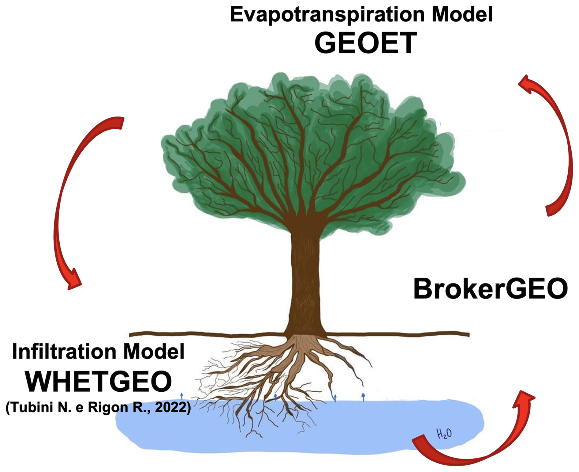
Figure 1 GEOSPACE-1D cycle path: presented graphically (designed by Concetta D'Amato) is the cyclic operation of GEOSPACE-1D, highlighting the crucial linkage among its three components. This feedback mechanism plays a key role in ensuring the mass and energy balance throughout the system.

GEOET (GEOframe EvapoTranspiration) is a suite of models that is designed to implement different formulations of ET, from the simplest Priestley–Taylor (PT) formula (Priestley and Taylor, 1972) to the complex computation of the energy budget at the canopy scale, as described in D'Amato and Rigon (2025).

Currently, GEOET, in addition to PT, incorporates the Penman–Monteith FAO model (PM-FAO) and the GEOframe–Prospero model (Bottazzi, 2020; Bottazzi et al., 2021). It is also designed to integrate more complex models that account for plant hydraulics, as implemented according to D'Amato and Rigon (2025). The presence of multiple models for computing evapotranspiration within a unified framework enables a comprehensive comparison of models and parameterizations, as they can leverage common auxiliary components. This possibility also meets the needs of users by offering a selection of modeling approaches of different levels of complexity, allowing users to choose according to their specific needs and available data. GEOET is also designed to implement the multiple water and environmental stress functions which are currently based on the Jarvis model (Macfarlane et al., 2004) and the Medlyn stomatal conductance model (Medlyn et al., 2011; Ball et al., 1987; Lin et al., 2015). Furthermore, GEOET models depth growth and root density functionally to understand soil–plant interactions in the process of root water uptake.

Finally, BrokerGEO is the coupler that allows the exchange of data between the other two components in memory, and it splits evaporation (E_s) and transpiration (E_l) between the control volumes in which the soil column is discretized.

The operational flow of the model follows a cyclic pathway, as illustrated in Fig. 1. Starting with WHETGEO-1D, GEOSPACE-1D computes the water suction for each control volume within the soil column. This information, integrated into the GEOET-StressFactor modules (further described in Sect. 5), plays a crucial role in determining the reduction in ET for each control volume, which is then consolidated into a global water stress factor value.

Furthermore, the GEOET-StressFactor modules incorporate additional reductions in ET associated with environmental variables, including air temperature, net radiation, and vapor pressure deficit, when necessary, in accordance with the selected method. The specific manner in which these stress factors are utilized varies depending on the chosen method or ET model, as detailed in Sect. 4, with the objective of limiting water abstraction from the soil.

Subsequently, BrokerGEO is responsible for partitioning the global Actual EvapoTranspiration (AET) into the soil control volumes using a root functioning model. Finally, an iterative process begins, during which WHETGEO, informed by the water evapotranspired from each control volume, recalculates the soil water potential, ensuring the conservation of both mass and energy budgets.

General notes about the software organization of GEOSPACE-1D

The macro-conceptual structure of GEOSPACE-1D is mirrored in a hierarchy of software entities. At a higher level are the OMS3 components (David et al., 2013, 2014). OMS3 is a component-based environmental modeling framework that empowers developers to create distinct components for individual modeling concepts. These components can be, in principle, executed and tested independently, thus establishing what could be called a secondary level of concern. A graphical example of a component is illustrated in Fig. 2. Each input parameter is sourced from a reader component or another component if derived from some modeling, while each output parameter is handled by a writer component. This setup facilitates straightforward management of data formats, streamlining the process for ease of use. Leveraging the modularity of OMS3, GEOSPACE-1D components integrate at runtime by connecting them with the OMS3 DSL based on Groovy (https://groovy-lang.org, last access: 19 December 2024). A standard operational configuration of the GEOSPACE-1D OMS3 components during runtime is depicted in Fig. 3, with simplification achieved by omitting all input/output connections for clarity.

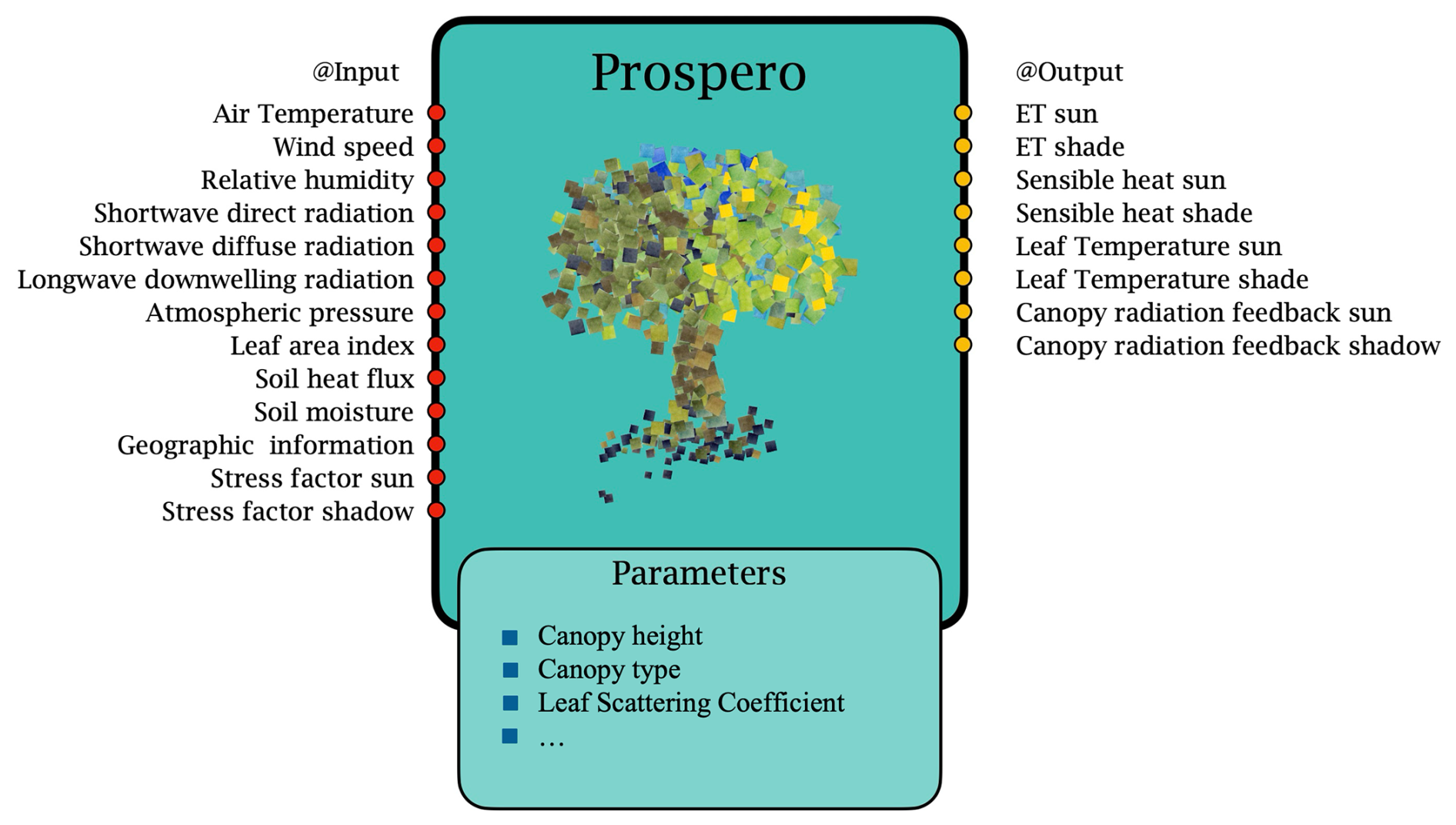
Figure 2 A pictorial representation of the Prospero OMS3 component with most of its inputs and outputs.

The GEOSPACE-1D system depicted in Fig. 3 consists of three main interconnected parts, each comprising a set of related components. WHETGEO actually has multiple variants, each distinguished by unique capabilities outlined in Tubini and Rigon (2022). More intricate is the GEOET, comprising five distinct components, each tasked with specific functions such as stress factor estimation, root modeling, soil evaporation estimation, and transpiration computation using, in this case, the Prospero model. Alternatively, a single component can replace the latter two and the one estimating the total evapotranspiration by employing, for instance, the Priestley–Taylor formula to estimate comprehensive evapotranspiration values. BrokerGEO employs two components in its connector role. The arrows denote variable flow among components, with thickness reflecting the volume of exchanged variables. For a comprehensive understanding of the complete workflow, we direct readers to examine the simulation configuration files provided in the Supplement, particularly the geospace1D_ProsperoPM.sim file. These .sim files, a standard feature of the OMS framework, serve as executable documentation that precisely records the model workflow, component connections, and parameter settings. The Supplement also includes a concise presentation with accompanying slides that provide detailed guidance on interpreting .sim file structure, component relationships, and execution sequence, offering valuable insights for both new users and those seeking to modify existing simulations.

OMS3, beyond the components, offers essential services, including tools for calibration and implicit parallelization of component runs. Further insights into the framework are available in the Supplement.

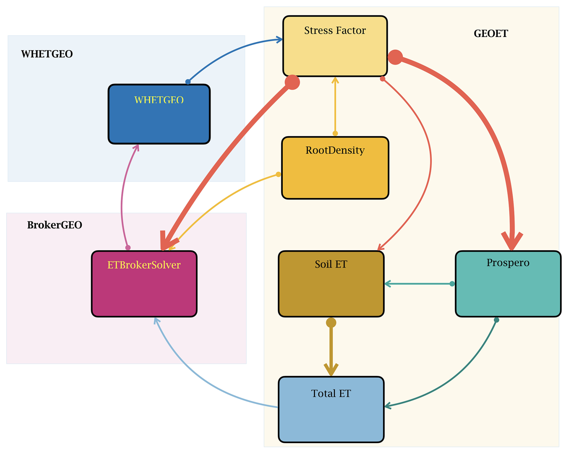
Figure 3 Here is an illustration of a simplified configuration in GEOSPACE-1D, focusing on component organization. We have omitted the components responsible for file I/O. One of the components, WHETGEO, exemplifies the various possibilities, differing in whether they account for the influence of the energy budget on flow. The simulations, as described in the text, begin with the WHETGEO component and progress according to the directional flow indicated by the arrows. The thickness of each arrow represents the number of variables exchanged between components, providing a visual indication of data transfer magnitude between system elements. For complete information on the workflow, please refer, for instance, to geospace1D_ProsperoPM.sim, which can be found in the Supplement.

Deeper within the software, written in Java programming language, it is organized into packages that encapsulate cohesive functional modules. The names of the packages formed are as follows:

• it.geoframe.blogspot.modelname.packagename

They are designed to avoid being confused with other models in the literature that implement the same classes. The site https://geoframe.blogspot.com/ (last access: 1 October 2025) is the blog where all the news and materials about GEOframe are posted, and the uniqueness of the URL guarantees that the names of the packages and classes are unique on the web. The contents of these packages are illustrated, for each of the three compartments, in the following sections.

A few software engineering choices were made and are characteristic “patterns” of the programming in GEOframe. Classes represent the finer programming level. In fact, internally, GEOSPACE-1D is coded with the Java language by organizing the various classes between interfaces and abstract classes. This adheres to the object-oriented principle “program to interfaces, not concrete classes”, facilitating the creation of scalable and maintainable software solutions. As stated earlier, reusability of the Java code is one of the prerogatives of the model. Therefore, we have adopted a generic programming approach (Berti, 2000) of decoupling the concrete data representation from the algorithm implementations by balancing it with specific approaches to improve the computational efficiency of the software. Because of these special programming structures, “patterns” are often used. In particular, the so-called Factory Pattern (Gamma et al., 1995) is used to instantiate at runtime the concrete classes chosen by the user among the various possibilities.

Because we are mostly interested in the implementation issues in this paper, we acknowledge a crucial aspect for facilitating information exchange between the soil and atmospheric compartments, which is how the data classes, i.e., the Java classes that manage the data quantities, are defined. These include the following.

• ProblemQuantities

• InputTimeSeries

• Parameters

These data classes serve as data containers and are managed distinctively from conventional OOP practices but similar to traditional scientific programming. They are mutable singleton static classes, instantiated once and serving as repositories for data updated at each time step. Further elaboration on these classes will be provided in the following sections.

3 WHETGEO

The first pillar of the GEOSPACE-1D modeling system is WHETGEO (Tubini and Rigon, 2022; Tubini et al., 2021). Its 1D deployment, WHETGEO-1D, is a new physically based model simulating the water and energy budgets in a soil column. It solves the conservative form of the Richardson–Richards equation, R² (Richards, 1931; Richardson, 1922), using the Newton–Casulli–Zanolli (NCZ) algorithm (Casulli and Zanolli, 2010) and also implements the numerical solution to solve the advection–dispersion equation by adopting the algorithm presented in Casulli and Zanolli (2005), currently applied to the heat transport. More comprehensive information about WHETGEO can be found in Tubini (2021), Tubini and Rigon (2022), and Tubini et al. (2021).

WHETGEO delves into infiltration and soil moisture dynamics that have cascading effects on various aspects of the environment, water resources, accurate water balance estimation, aquifer recharge prediction, and flow patterns.

For what regards evaporation, it is well-established that plant productivity is significantly influenced by the patterns of soil moisture dynamics (Porporato et al., 2004). Soil moisture deficit, in particular, reduces plant water potential, inducing water stress, which can lead to dehydration, loss of turgor, xylem cavitation, stomatal closure, and a decrease in photosynthesis (Nilsen and Orcutt, 1996). At the same time, it is an oversimplification to model soil moisture dynamics without considering transpiration, which constitutes a significant portion of the water budget. The relationship between soil moisture and evapotranspiration is a crucial component for accurately representing soil water balance. Regardless of the specific ET model used, it is the amount of water extracted from the soil at various depths by plant roots (Evaristo and McDonnell, 2017). These roots are capable of absorbing substantial amounts of water, significantly altering the distribution of the water column.

An approach to include the evapotranspiration flux within the soil moisture dynamics is to add a sink term representing water extraction by plant roots in the R² equation, obtaining a modified one-dimensional continuity equation (Feddes et al., 1976; Molz, 1981):

$$\begin{array}{}\text{(1)}& {\displaystyle \frac{\partial \mathit{\theta }}{\partial t}}+S_{\mathrm{s}}{\displaystyle \frac{\mathit{\theta }}{{\mathit{\theta }}_{\mathrm{s}}}}{\displaystyle \frac{\partial \mathit{\psi }}{\partial t}}=\mathrm{\nabla }\cdot \left(K\left(\mathit{\theta }\right)\mathbf{\nabla }\left(\mathit{\psi }+z\right)\right)-S\left(z\right)+R\left(z\right),\end{array}$$

where the forces acting are gravity z [L] and the matric potential ψ [L]. In Eq. (1), K [L T⁻¹] is the hydraulic conductivity, θ [–] is the dimensionless volumetric water content, ∇ [L⁻¹] is the gradient operator, z [L] is the vertical coordinate, positive upward, S is the water extraction function [T⁻¹], and R [T⁻¹] is the water redistribution function by roots. The function S(z) represents water extraction by plant roots and can depend on space, time, root density distribution, water potential, water content, or a combination of these variables (Feddes et al., 1976; Perrochet, 1987; Lai and Katul, 2000). S_s [L⁻¹] is the specific storage coefficient, defined as

$$\begin{array}{}\text{(2)}& S_{\mathrm{s}}=\mathit{\rho }g(n\mathit{\beta }+\mathit{\alpha }),\end{array}$$

with ρ [M L⁻³] being the water density, g [L T⁻²] the gravitational acceleration, n [L³L⁻³] the soil porosity, β [L T² M⁻¹] the liquid compressibility, and α [L T² M⁻¹] the soil matrix compressibility.

Molz and Remson (1970) highlight the impracticality of modeling water transport in soil with complex root systems considering flow to individual rootlets. Precise root geometry is hard to measure and varies over time. Additionally, root water permeability changes along their length, noted by Kramer (1970). Consequently, the extraction function S(z) is treated with simplified models which adopt a macroscopic, not microscopic, approach, which is actually computed by the BrokerGEO components (described in Sect. 6).

Like source term models, the roots themselves are capable of redistributing water between different soil layers (Beyer et al., 2018), but the modeling of the source term R(z) is not under scrutiny in this paper.

Extension of the Richards solver, i.e., on the RichardsRootSolverMain

The algorithmic concepts of WHETGEO are comprehensively described in Tubini and Rigon (2022), but here, we summarize only those aspects related to the extension we made for allowing the connection with GEOET and BrokerGEO.

In WHETGEO, the column of soil is discretized in layers, which are parts of the soil column with the same soil type, and control volumes, which are finite-volume elements, in which the R² equation is solved. Each control volume is characterized by geometrical quantities grouped into a parameter set, which contains all the parameters controlling the flow dynamics and defining the form of the equations to be solved. These parameters are specific to each control volume. All of this information is stored in the grid file and, once read, is stored in the Geometry and ProblemQuantities, singleton classes as illustrated in Fig. 4.

A more detailed examination of Fig. 4 reveals that ProblemQuantities and Geometry are typical example of “reflexive association”, a type of relationship between elements in a class diagram where an element is associated with itself. In other words, it is an association between instances of the same class and it means that the class could work stand-alone. The term S(z) in Eq. (1) is a sink which affects any layer, and this can be obtained by means of the introduction of some new classes.

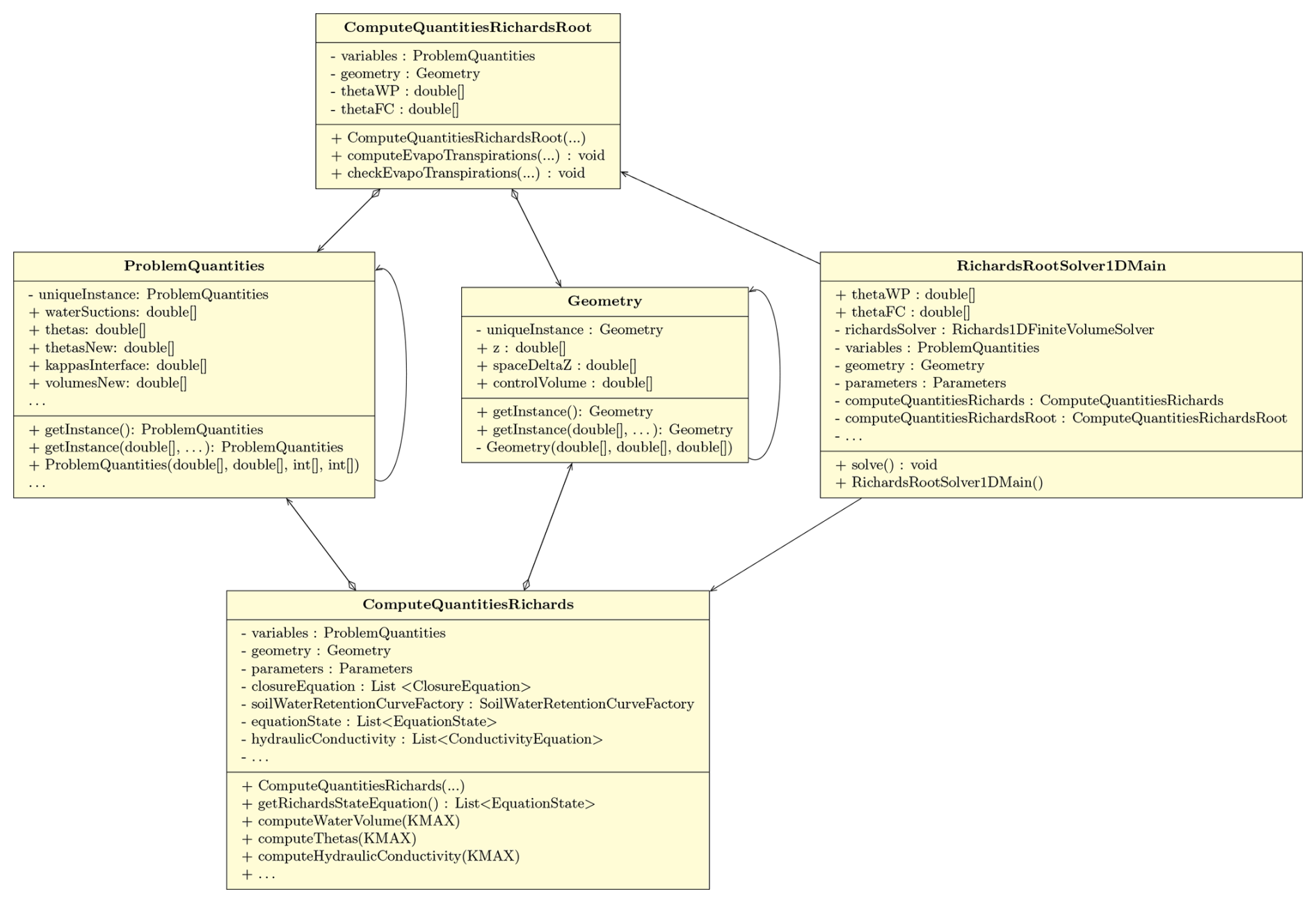
Figure 4 UML class diagram for the RichardsRootSolver1DMain class. The class solves Eq. (1) directly by calling the methods of the concrete classes ComputeQuantitiesRichardsRoot and ComputeQuantitiesRichards.

The first class that has been added is the following.

• ComputeQuantitiesRichardsRoot

ComputeQuantitiesRichardsRoot is a Java class with the responsibility of managing the evapotranspiration demand for each control volume, sourced from BrokerGEO. Its primary function involves assessing the requested water volume against the available water content in each control volume, thereby estimating the reduction in ET and deriving a stress factor, $g_{{\mathrm{w}}_i}$, for every soil layer. These stress factors are subsequently utilized iteratively to determine the actual evapotranspiration (AET) through information exchange with GEOET via BrokerGEO. AET is then deducted from each control volume, with the class overseeing algorithm convergence as well.

A closer inspection of Fig. 4 reveals that the ComputeQuantitiesRichardsRoot class is composed by aggregation with the ProblemQuantities class and the Geometry class as mentioned above. The first one contains all the variables of the models and its implementation using the singleton pattern (Freeman, 2004), whereas the second one manages the geometric features of the grid and how grid elements are connected to each other.

While the present deployment of GEOSPACE works in a 1D column, it is ready to manage the more complex topologies of 2D or 3D future versions of the system.

The relationship between the classes ComputeQuantitiesRichardsRoot and ProblemQuantities can be described as a combination of both “association” and “aggregation” (Fowler, 2004). The ComputeQuantitiesRichardsRoot class maintains a reciprocal “association” with the ProblemQuantities class through the instantiated variables, allowing them to interact and exchange information. Furthermore, an “aggregation” relationship exists where the ComputeQuantitiesRichardsRoot class encapsulates an instance of the ProblemQuantities class to manage and compute various problem-related quantities, as illustrated by an empty diamond shape (Fig. 4). Overall, this relationship structure enhances the modularity and organization of the software design, enabling the ComputeQuantitiesRichardsRoot class to efficiently utilize and manage the data provided by the ProblemQuantities class.

The class involved in solving Eq. (1) considering the amount of water removed by evapotranspiration is the concrete class, RichardsRootSolver1DMain, as shown in the UML (Unified Modeling Language) diagram of Fig. 4.

The RichardsRootSolver1DMain class, as shown in Fig. 4, is directly connected with ComputeQuantitiesRichardsRoot and ComputeQuantitiesRichards and with their methods to compute the solution of the pressure value ψ at any time step. In this specific case, the RichardsRootSolver1DMain class uses ComputeQuantitiesRichardsRoot, and the actual solver is the solve() method, which contains the solving algorithms. With the change of each of the “Compute” classes, this abstract structure allows changing the solver type by just adding some new class in substitution.

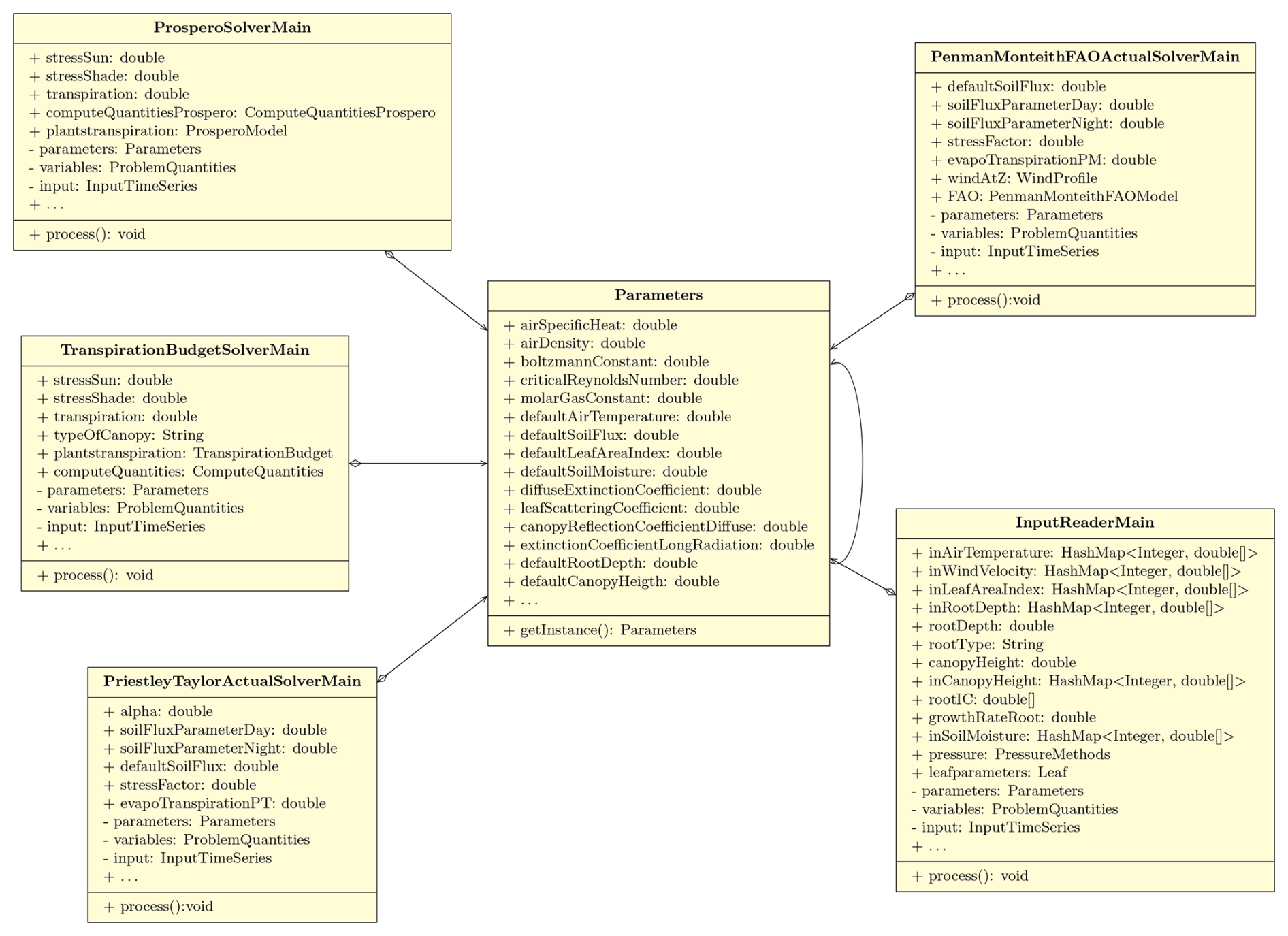
Figure 5 UML class diagram of the Parameters class, illustrating its aggregation and association relationships with the ET model solvers and the input reader class.

4 GEOET

The process of plant transpiration propels the exchange of water and energy between the Earth's surface and the atmosphere (Katul et al., 2012). This phenomenon significantly impacts the uptake of carbon by the ecosystem and also plays a pivotal role in determining how rainfall infiltrates into the soil and the moisture profile dynamic. In fact, the interaction between soil evaporation and plant transpiration is not merely a sum of physical processes but is influenced by feedback mechanisms. As plants transpire, they create a suction that draws moisture from the soil into their root systems, thereby influencing the rate of soil evaporation. Conversely, soil evaporation can reduce the available moisture for plant roots, impacting their ability to transpire effectively. This dynamic coupling shapes the moisture profile within the soil, significantly changing the overall water availability for the soil and vegetation and for the entire hydrological cycle.

The GEOET system incorporates three evapotranspiration models, as illustrated in Fig. 6. In the following the formulas that implement them are reported for readers' convenience. First comes the Priestley–Taylor one (Priestley and Taylor, 1972), secondly the Penman–Monteith FAO (Penman and Keen, 1948), and lastly the Prospero model (Bottazzi, 2020; Bottazzi et al., 2021). As described in Appendix A, Prospero solves the stationary energy budget coupled with water vapor transport and sensible heat transport using a zeroth-order approximation, incorporating information derived from the Clausius–Clapeyron equation. A comprehensive step-by-step derivation of the solution method is presented in D'Amato and Rigon (2025), which also addresses its current limitations and discusses potential enhancements. While the envisioned improvements are not yet implemented in the current GEOSPACE design, the software architecture has been carefully structured to accommodate future implementation of these and other advanced features.

The Priestley–Taylor ET estimator

The Priestley–Taylor model component (PT) (Priestley and Taylor, 1972) is based on the formula

$$\begin{array}{}\text{(3)}& {\mathrm{ET}}_{\mathrm{PT}}=\mathit{\alpha }{\displaystyle \frac{\mathrm{\Delta }}{(\mathrm{\Delta }+\mathit{\gamma })}}(R_{\mathrm{n}}-G),\end{array}$$

where α is an empirical coefficient relating actual evaporation to equilibrium evaporation, Δ is the slope of the saturation vapor pressure and air temperature curve [kPa °C⁻¹], γ is the psychrometric constant [kPa °C⁻¹], R_n is the net radiation [W m⁻²], and G is the ground heat flux [W m⁻²].

The implementation of this formula is relatively straightforward, although the radiation term requires a more detailed and careful evaluation. Further information about this equation can be found in Appendix A.

The Penman–Monteith FAO estimator

The second model presently implemented is the Penman–Monteith FAO approximation (PM) (Penman and Keen, 1948), an adaptation of the Penman–Monteith model, as outlined in the following equation (Allen, 1986):

$$\begin{array}{}\text{(4)}& {\mathrm{ET}}_{\mathrm{0}}={\displaystyle \frac{\mathrm{1}}{\mathit{\lambda }}}{\displaystyle \frac{\mathrm{0.408}\mathrm{\Delta }(R_{\mathrm{n}}-G)+\mathit{\gamma }\frac{\mathrm{900}}{T+\mathrm{273}}{u}_{\mathrm{2}}{\mathit{\delta }}_{\mathrm{a}}}{\mathrm{\Delta }+\mathit{\gamma }(\mathrm{1}+\mathrm{0.34}{u}_{\mathrm{2}})}},\end{array}$$

where ET₀ is the reference evapotranspiration [mm d⁻¹], R_n is the net radiation at the crop surface [MJ m⁻² d⁻¹], G is the soil heat flux density [MJ m⁻² d⁻¹], T is the mean daily air temperature at 2 m height [°C], u₂ is the wind speed at 2 m height [m s⁻¹], e_s is the saturation vapor pressure also known as vapor pressure at the dew point [kPa], e_a [kPa] is the actual vapor pressure, ${\mathit{\delta }}_{\mathrm{a}}=(e_{\mathrm{s}}-e_{\mathrm{a}})$ [kPa] is the saturation vapor pressure deficit, and Δ [kPa °C⁻¹] is the derivative of the Clausius–Clapeyron formula.

In terms of computational complexity, these models are relatively straightforward. Both PT and PM are equipped with dedicated packages housing their respective core Java classes for solving the equations, PriestleyTaylorModel.java and PMFAOModel.java. Additionally, each package includes various “solver” classes designed to invoke methods from the main model class, enabling the computation of solutions that account for environmental inputs and stress factors.

Specifically, to ensure that users do not input more information than necessary or provide data unrelated to their chosen method, we differentiate between solvers for calculating potential evapotranspiration (without stresses) and actual evapotranspiration (with the possibility to select among the various type of stresses).

The Prospero model

The Prospero model (Bottazzi, 2020; Bottazzi et al., 2021) is a physically based approach for calculating transpiration as detailed in D'Amato and Rigon (2025). The transpiration, E_l, is considered for the sunlit and shaded fractions of the canopy while the soil evaporation, E_s, is estimated using the residual radiation hitting the soil. E_s, at present, is determined according to the FAO Penman–Monteith model, i.e., E_s=ET₀. Meanwhile, E_l is computed using the Prospero model that implements a modified version of the Schymanski and Or (SO) model (Schymanski and Or, 2017), which has been upscaled to address canopy-level transpiration and ensure mass conservation during periods of water stress.

This model returns not only an E_l estimate but also the sensible heat H and vapor pressure gap e_Δ, besides the temperature of the leaves, T_l. The latter variable is the key for obtaining the others, as below:

$$\begin{array}{}\text{(5)}& T_{\mathrm{l}}={\displaystyle \frac{\begin{array}{c}{R}_{\mathrm{n}}+a_{\mathrm{sH}}{A}_{\mathrm{tr}}{\mathit{ϵ}}_{\mathrm{l}}\mathit{\sigma }{T}_{\mathrm{a}}^{\mathrm{4}}+c_{\mathrm{H}}(a_{\mathrm{sH}},A_{\mathrm{tr}})\cdot T_{\mathrm{a}}\\ +c_{\mathrm{E}}(a_{\mathrm{sE}},A_{\mathrm{tr}},g_{\mathrm{s}})\cdot (\mathrm{\Delta }\cdot T_{\mathrm{a}}+{\mathit{\delta }}_{\mathrm{a}})\end{array}}{c_{\mathrm{H}}(a_{\mathrm{sH}},A_{\mathrm{tr}})+c_{\mathrm{E}}(a_{\mathrm{sE}},A_{\mathrm{tr}},g_{\mathrm{s}})\mathrm{\Delta }+a_{\mathrm{sH}}{A}_{\mathrm{tr}}{\mathit{ϵ}}_{\mathrm{l}}\mathit{\sigma }{T}^{\mathrm{3}}}},\end{array}$$

where R_n is the net radiation, a_sH represents the sides of surface exchanging sensible heat and longwave radiation (equal to 1 for single-layer exchange, 2 for two-layer exchange such as leaves [–]), A_tr is the transpiring surface for a unit of ground surface [–], ϵ_l [–] is the leaf emissivity, $\mathit{\sigma }=\mathrm{1.67}\times {\mathrm{10}}^{-\mathrm{8}}$ [$\mathrm{W}{\mathrm{m}}^{-\mathrm{2}}{\mathrm{K}}^{-\mathrm{4}}$] is the Stefan–Boltzmann constant, a_sE represents the sides of surface exchanging latent heat (equal to 1 for hypostomatous and 2 for amphistomatous [–]), g_s is the stomatal conductance [m s⁻¹], δ_a=P_ws and P_w are the saturation water vapor pressure and the water vapor pressure, respectively, c_E is the total conductance for water vapor evapotranspiration transport [m s⁻¹], and c_H is the total conductance for the sensible heat transport [m s⁻¹].

It is assumed that the right-hand-side terms in Eq. (5) are all known. Furthermore, the water pressure gap is estimated as follows.

$$\begin{array}{}\text{(6)}& e_{\mathrm{\Delta }}:=e_{\mathrm{s}}-e_{\mathrm{l}}=\mathrm{\Delta }(T_{\mathrm{l}}-T_{\mathrm{a}})+{\mathit{\delta }}_{\mathrm{a}}\end{array}$$

The transpiration is calculated as

$$\begin{array}{}\text{(7)}& E_{\mathrm{l}}=c_{\mathrm{E}}(a_{\mathrm{sE}},A_{\mathrm{tr}})e_{\mathrm{\Delta }}.\end{array}$$

Finally, the sensible heat is computed as

$$\begin{array}{}\text{(8)}& H_{\mathrm{l}}=c_{\mathrm{H}}(a_{\mathrm{sH}},A_{\mathrm{tr}})(T_{\mathrm{l}}-T_{\mathrm{a}}).\end{array}$$

For further information on these formulas or solutions, please refer to Bottazzi (2020), Bottazzi et al. (2021), or D'Amato and Rigon (2025).

4.1 The GEOET informatics organization

The evapotranspiration component, GEOET, developed as part of this paper, is based on its precursor, the GEOframe-ETP model (Bottazzi, 2020; Bottazzi et al., 2021), whose original source code is available at https://github.com/geoframecomponents/ETP (last access: 1 October 2025). Both GEOframe-ETP and GEOET simulate the evapotranspiration according to different evapotranspiration models: the Priestley–Taylor model (Priestley and Taylor, 1972), the Penman–Monteith FAO model (Allen et al., 1998), and the GEOframe–Prospero model (Bottazzi, 2020; Bottazzi et al., 2021). But, in moving from one software to the other, the refactoring of the existing codes was substantial at both the design level and algorithmic level, as you can see in the box diagrams of Fig. 6. The reorganization and the re-engineering of the software were essential to allow the use of multiple options of evapotranspiration physics to introduce a separate component for calculating the stress factor, making it possible to apply them to all evapotranspiration models and facilitating the connection of any of the ET components with other model components, particularly enabling its linkage with WHETGEO.

The new version of the code thus allows the physical processes of evapotranspiration to be analyzed individually and also in conjunction with the infiltration process. To obtain this, as shown in Fig. 6, all the evapotranspiration models were separated into packages of classes with specific tasks. Furthermore, depending on the model's complexity, each package is hierarchically organized into additional packages and classes. Each class is designed to perform a singular task and strives to be as self-contained as possible. This design not only ensures that each class operates independently but also shields the user from the need to provide inputs or information unrelated to the specific model they are utilizing.

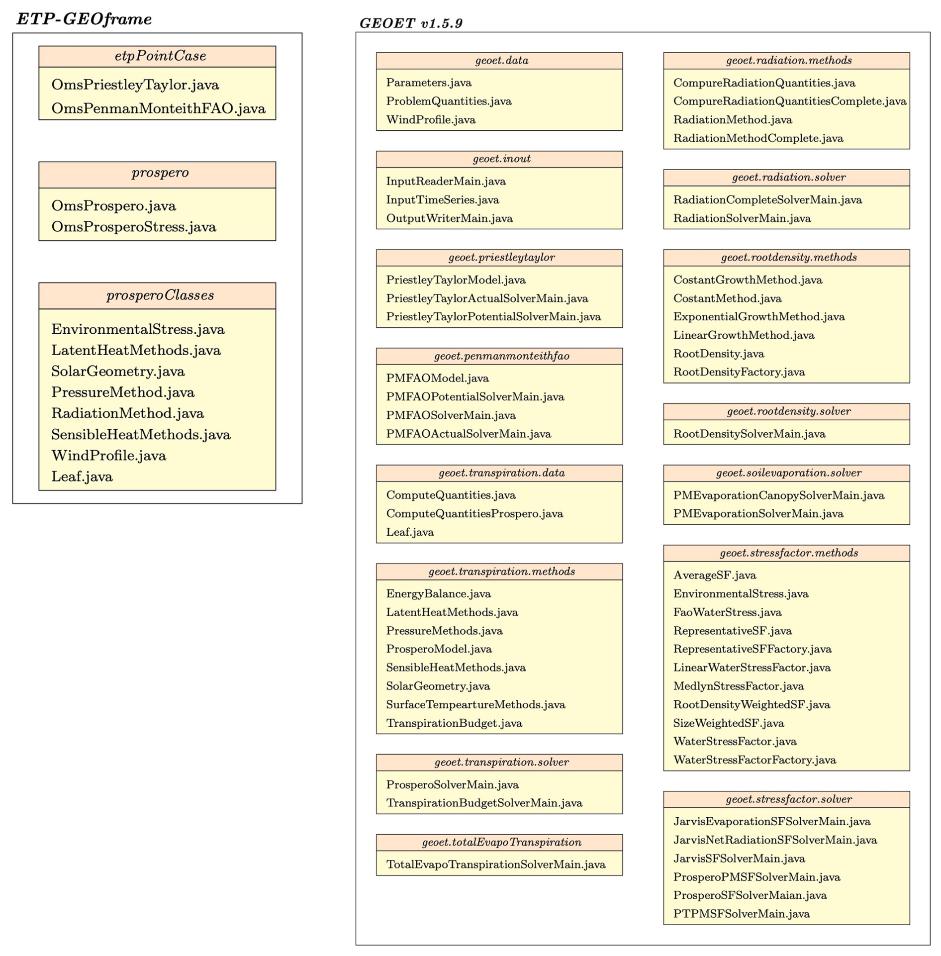
Figure 6 The GEOframe ET original packages, constituting ETP-GEOframe (Bottazzi, 2020) (on the left), and the new packages (on the right) containing in GEOET. This refactoring was necessary to accommodate multiple options for estimating the water stress factor, to incorporate a more sophisticated radiation budget, and to integrate a model for root functioning.

The new packages include the following.

• geoet.data is the package responsible for managing the data and variables of all the ET models. The data are encapsulated in singleton static classes that are simultaneously available to all the other classes of estimating ET, as previously described for the data classes functional to WHETGEO.

• geoet.inout package was crafted to facilitate the management of model inputs and outputs, as the model's evolution aligns with contemporary trends to separate model-agnostic data from the models themselves. This software structure, in fact, allows for the incorporation of diverse data ingestion and extraction methodologies and is pivotal in harnessing novel data-handling advancements as they emerge.

Besides the packages dedicated to ancillary shared tasks, packages were dedicated to containing the various algorithms for each of the evapotranspiration estimation models used.

• The Priestley–Taylor formulation (Priestley and Taylor, 1972) of ET is implemented in the geoet.priestleytaylor package.

• The Penman–Monteith FAO model is implemented in the geoet.penmanmonteithfao package.

• The Prospero model is more conceptually and computationally complex than the other two models and, as can be seen in Fig. 6, is split into various packages. The relative packages are named geoet.transpiration.*.

A specialized package has been developed exclusively for estimating the soil evaporation, designated as geoet.soilevaporation.solver. In this phase, the computation of soil evaporation employs the Penman–Monteith method. However, the software's architecture is designed to facilitate effortless integration and development of novel techniques based on the theory supported by the work by Lehmann et al. (2014).

Enclosed within the geoet.radiation.* packages are the procedures inherited from the earlier ETP-GEOframe version, alongside the methodologies introduced in this study, expounded in the Supplement, which build upon the parameterizations of the processes delineated in De Pury and Farquhar (1997) and Ryu et al. (2011).

4.1.1 How to add a new model?

A primary objective in the software engineering of the GEOSPACE system was to enable feature expansion through class addition rather than code modification, adhering to the open–closed principle of object-oriented design. By following the OOP and generic programming principles of GEOSPACE-1D, integrating a new model component, either a solver or a new stress function, into the existing code base becomes, in fact, straightforward. To illustrate that this feature can actually be applied to any part of GEOSPACE, consider the introduction of a new stress model. To incorporate it, a concrete class is created within the geoet.stressfactor.methods package, such as HydroDemo.java, where the numerical equation for the new method is defined. Furthermore, a solver class is developed within the geoet.stressfactor.solver package, for instance HydroDemoSolverMain.java. This class solves the equation by directly invoking methods from the concrete classes. This integration is achieved through addition, requiring no modifications to previously written code.

The newly created class, HydroDemo.java, extends the existing abstract class, WaterStressFactor.java (see Sect. 5.4). This new class provides the implementation of the concrete method defined in the abstract class and inherits all of its characteristics. Finally we update the file WaterStressFactorFactory.java with the string that users must enter in the model executable to specify the new method they wish to use, namely “HydroDemo”.

5 About the stress factor models and their deployment

As highlighted in the Supplement, the modeling of stomatal conductance, often referred to as the “vegetation stress factor”, is a central subject of debate within the scientific literature. This contentious issue has spurred the emergence of multiple theoretical frameworks, each trying to provide a comprehensive understanding of this intricate physiological process (Daly et al., 2004).

It is essential to have a computer modeling framework that facilitates the integration of emerging theories without compromising the integrity of the current code. This capability of GEOSPACE-1D ensures that it can adapt in harmony with new research advancements, thereby enhancing the resilience and relevance of its computational framework.

The scientific literature reveals two primary families of parameterizations governing leaf conductance (Yu et al., 2017), the Jarvis model (Jarvis et al., 1976) and the Ball–Berry one (Dewar, 2002), and it is pivotal to create an informatics infrastructure capable of implementing both these formulations. To achieve this, we constructed an adaptable set of packages: geoet.stressfactor.*.

The forthcoming implementation we are detailing must seamlessly function with both the GEOET model independently and when integrated with GEOSPACE-1D. In each scenario, it should have the flexibility to accommodate different stress factor models. This abstraction is essential as stress factor data pertaining to each control volume are not only crucial for GEOET but also necessary for BrokerGEO and WHETGEO within the GEOSPACE-1D framework. So far, two stress parameterizations have been implemented, the so-called Jarvis model (Jarvis et al., 1976; Macfarlane et al., 2004; White et al., 1999) and the Medlyn stomatal conductance model (Medlyn et al., 2011).

5.1 The Jarvis model for stresses

As described in the Supplement, the Jarvis model implemented in GEOET follows the formulation proposed by White et al. (1999) and Macfarlane et al. (2004), where stomatal conductance is given by

$$\begin{array}{}\text{(9)}& g_{\mathrm{s}}=g_{\mathrm{s},\max }\cdot f_R\left(R_{\mathrm{PAR}}\right)\cdot f_T\left(T_{\mathrm{a}}\right)\cdot f_{\mathit{\delta }}\left({\mathit{\delta }}_{\mathrm{a}}\right)\cdot f_{\mathit{\psi }}\left({\mathit{\psi }}_{\mathrm{l}}\right).\end{array}$$

Here, the stress reduction functions f account for photosynthetically active radiation (PAR) f_R(R_PAR), air temperature f_T(T_a), vapor pressure deficit f_δ(δ_a), and leaf water potential f_ψ(ψ_l). All details about the functional forms used for each f are provided in the Supplement, and their implementation is available in the EnvironmentalStress.java class.

As regards the water stress, despite the wealth of literature, in a considerable number of soil–plant models, water availability directly depends on θ (Verhoef and Egea, 2014a) rather than on ψ. Following what was done in the precursor GEOframe-ETP model (Bottazzi, 2020), we maintained the FAO water stress factor K_s (Appendix A) and a new formulation was added as a function f_θ(θ), the “fraction of transpirable soil water” (FTSW), to be used in the Jarvis model (Eq. 9). The formula itself is a representation of the relationship between soil moisture content (θ), wilting point (θ_WP), and field capacity (θ_FC), and it is commonly used to assess plant water stress and to make decisions related to irrigation management and water conservation. The Java class involved in the computation of the FTSW is the LinearWaterStressFactor.java class and computes the water stress factor in each control volume of the grid computational soil according to the following:

$$\begin{array}{}\text{(10)}& g_{\mathrm{w},i}={\displaystyle \frac{{\mathit{\theta }}_i-{\mathit{\theta }}_{\mathrm{WP},i}}{{\mathit{\theta }}_{\mathrm{FC},i}-{\mathit{\theta }}_{\mathrm{WP},i}}},\end{array}$$

where g_w,i is the water stress factor in the ith control volume; θ_i represents the current soil water content in the ith control volume; θ_WP,i is the wilting point of the ith control volume of the soil, which is the moisture level at which plants can no longer extract water from the soil effectively, leading to wilting; and θ_FC,i represents the field capacity of the ith control volume of the soil, which is the maximum amount of water the soil can hold against the force of gravity.

The θ_i value derived from the WHETGEO model, and likewise the parameters θ_WP,i and θ_FC,i, is customized for each control volume, as it is the user's choice to discretize the soil column and determine the number of layers and associated parameter values. Consequently, the values of θ_WP,i and θ_FC,i are specific to each individual soil layer and, by extension, to all the control volumes containing them.

5.2 The Medlyn model for stresses

The Medlyn model (Medlyn et al., 2011) is part of the Ball–Berry–Leuning (BBL) family of models (Ball et al., 1987; Leuning, 1990; Dewar, 2002), and it has been modified in various ways since the original paper. For instance, in Dewar (2002) the form given to it is

$$\begin{array}{}\text{(11)}& g_{\mathrm{B}}=g_{\mathrm{0}}+g_{\mathrm{1}}{\displaystyle \frac{A_{\mathrm{n}}}{(C_{\mathrm{s}}-\mathrm{\Gamma })\left(\mathrm{1}+\frac{{\mathit{\delta }}_{\mathrm{a}}}{e_{\mathrm{0}}}\right)}},\end{array}$$

where g_B is the Ball–Berry–Leuning conductance, g₀ is the value of g_B at the light compensation point, g₁ and e₀ are empirical coefficients, A_n is the net leaf CO₂ assimilation rate, C_s is the CO₂ concentration at the leaf surface, Γ is the CO₂ concentration at the compensation point, and finally δ_a is the water vapor pressure deficit.

An interesting form of the BBL was obtained in Medlyn et al. (2011), under the hypothesis of optimal photosynthesis theory, which is

$$\begin{array}{}\text{(12)}& g_{\mathrm{B}}=\mathrm{1.6}\left(\mathrm{1}+{\displaystyle \frac{g_{\mathrm{1}}}{\sqrt{{\mathit{\delta }}_{\mathrm{a}}}}}\right){\displaystyle \frac{A_{\mathrm{n}}}{C_{\mathrm{s}}}}.\end{array}$$

Equation (12) has been integrated into the GEOSPACE-1D framework simply by adding a class,

• MedlynStressFactor.java,

and it is fully functional when a time series of net carbon assimilation is provided as input. Its scope is actually to be a placeholder for a future OMS3 component dedicated to computing net carbon assimilation within GEOSPACE-1D.

5.3 Estimating the global stress on the basis of local stresses

Given the discretization of soil into multiple layers within GEOSPACE-1D, it becomes imperative to establish a method for distributing total stress estimates based on local stresses and reciprocally allocating transpiration demands across these soil layers. The mechanism through which soil moisture is transported into plants, thereby facilitating E_l, is primarily via the roots (Carminati and Javaux, 2020). Hence, despite its simplicity, the introduction of a root functioning model is essential. Within GEOSPACE-1D, root models are integrated into GEOET through the following.

• geoet.rootdensity.methods package

• geoet.rootdensity.solver package

Eventually, at this point, the information derived by the root models can be used to estimate the total stress acting on the plants. GEOET implements three ways to estimate the global stress called the average water stress factor, the size-weighted stress factor, and the root-density-weighted water stress factor, which are briefly described below.

• The average water stress factor is implemented in the AverageSF.java class, according to which the representative water stress factor value at the nth instant, G_w, is given by the arithmetic mean of the stress values characterizing the soil column:

  $$\begin{array}{}\text{(13)}& G_{\mathrm{w}}={\displaystyle \frac{{\sum }_{i=\mathrm{1}}^N{g}_{\mathrm{w},i}}{N}},\end{array}$$

  where N is the total number of control volumes affected by the roots.

• The size-weighted water stress factor is implemented in the SizeWeightedSF.java class, according to which the representative water stress factor value at the nth instant, G_w, is given by the weighted average of the water stress values characterizing the soil column as a function of the size dx of the control volumes affected by the roots:

  $$\begin{array}{}\text{(14)}& G_{\mathrm{w}}={\displaystyle \frac{{\sum }_{i=\mathrm{1}}^N{g}_{\mathrm{w},i}\cdot {\mathrm{dx}}_i}{{\sum }_{i=\mathrm{1}}^N{\mathrm{dx}}_i}}={\displaystyle \frac{{\sum }_{i=\mathrm{1}}^N{g}_{\mathrm{w},i}\cdot {\mathrm{dx}}_i}{{\mathit{\eta }}_{\mathrm{R}}}}.\end{array}$$

  It is specified that the sum of the size dx_i of the control volumes affected by the root system coincides with the depth η_R of the roots themselves.

• The root-density-weighted water stress factor is implemented in the RootDensityWeightedSF.java class, according to which the representative water stress factor value at the nth instant, G_w, is given by the weighted average of the water stress values characterizing the soil column as a function of the root density ρ_R,i of the control volumes affected by the roots:

  $$\begin{array}{}\text{(15)}& G_{\mathrm{w}}={\displaystyle \frac{{\sum }_{i=\mathrm{1}}^N{g}_{\mathrm{w},i}\cdot {\mathit{\rho }}_{\mathrm{R},i}}{{\sum }_{i=\mathrm{1}}^N{\mathit{\rho }}_{\mathrm{R},i}}}={\displaystyle \frac{{\sum }_{i=\mathrm{1}}^N{g}_{\mathrm{w},i}\cdot {\mathit{\rho }}_{\mathrm{R},i}}{{\mathit{\rho }}_{\mathrm{Root}}}}.\end{array}$$

  In this case the sum of the root density in each control volume ρ_R,i affected by the root system coincides with the total root density in the root zone ρ_Root.

5.4 Informatics: factory pattern for stress estimator

The many parameterizations in the literature for the calculation of the stomatal conductance, as well as the numerous formulations that can be used for the computation of a representative stress factor value, pose precisely the problem of how to implement a structure that is flexible to current and future changes. To do this, we relied on the potential of the design, i.e., the simple factory pattern (Gamma et al., 1995). If we consider the case of the computation of the representative water stress factor value, we practically need different subclasses that implement several methods with the possibility for the user to choose one of these classes and also add new method in the future. Indeed, employing the simple factory pattern (Freeman, 2004; Gamma et al., 1995) enables the encapsulation of object creation logic within the factory class.

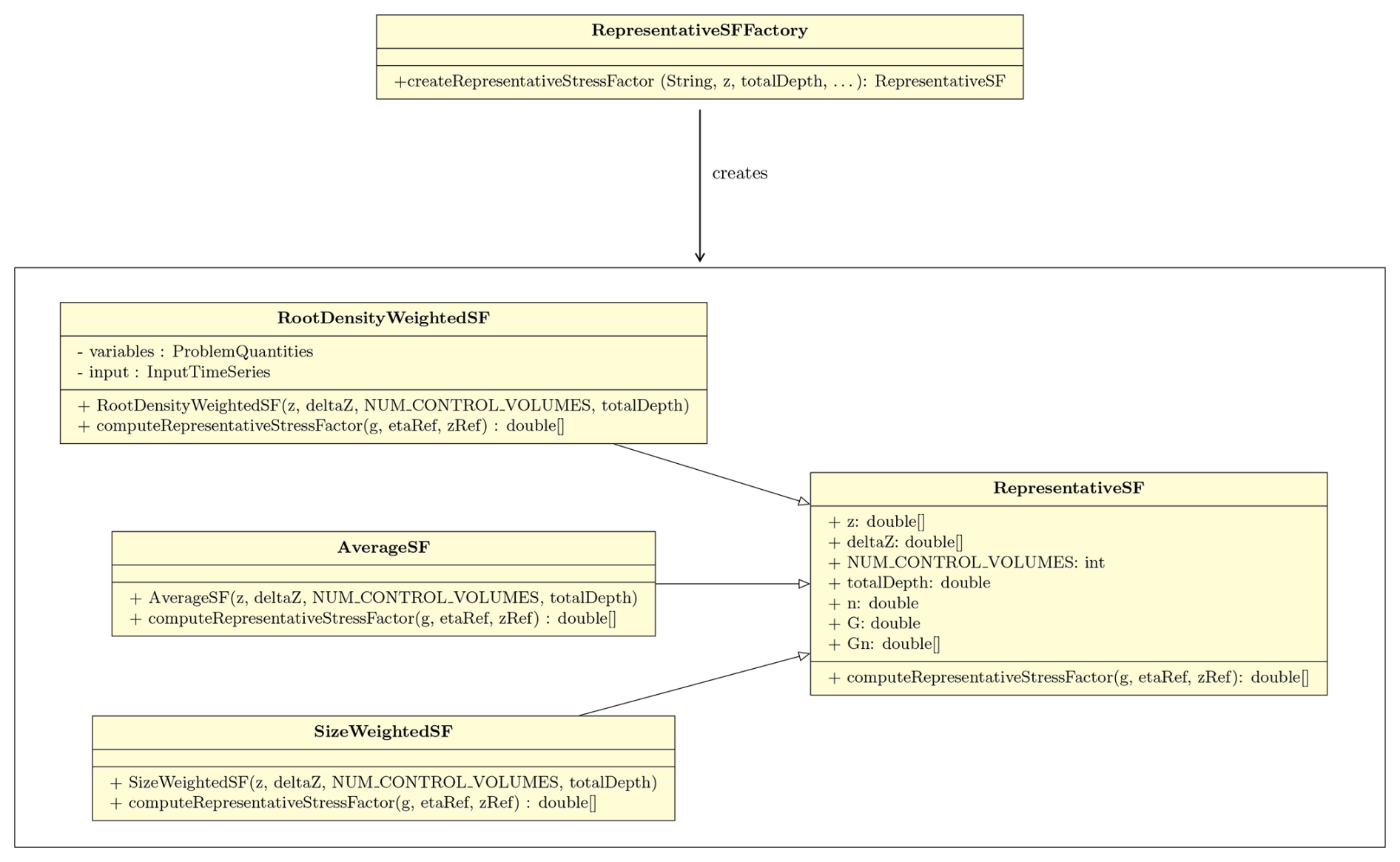
Figure 7 UML class diagram for the Java simple factory applied for the choice of the representative water stress factor computation model. The RepresentativeSF class defines the interface that is implemented by the concrete classes RootDensityWeightedSF, AverageSF, and SizeWeightedSF.

As shown in Fig. 7, the RepresentativeSF class is an abstract class and three Java classes that implement the concrete methods to compute the representative water stress factor:

• RootDensityWeightedSF,

• AverageSF,

• SizeWeightedSF.

A closer inspection of Fig. 7 reveals that the RepresentativeSFFactory class accomplishes the task of implementing one of the concrete classes. In particular, the RepresentativeSFFactory class is responsible for creating instances of RepresentativeSF or its subclasses based on a specified type provided as input. The RepresentativeSFFactory class is connected to the classes RepresentativeSF and its possible subclasses through the createRepresentativeStressFactor method. The factory creates instances of RepresentativeSF or its subclasses based on the specified type and returns them as output.

In the context of computing water stress within each control volume, an abstract and factory class framework was developed, like the one just described, using the Java classes WaterStressFactor and WaterStressFactorFactory. This architecture was designed with the foresight of accommodating novel formulations.

6 BrokerGEO actions and packages

It is important to note that the ET (or T) flux drawn from the soil from each control volume estimated by GEOET is subject to a water stress which depends on the existing water content estimated by WHETGEO, establishing a feedback between the two software components. To implement the feedback, BrokerGEO distributes the evaporative demand among the soil control volumes. The three methods implemented below mirror the methods used to obtain the global water stress factor in GEOET for any time step.

• Average water-weighted method

  $$\begin{array}{}\text{(16)}& {\mathrm{ET}}_{\mathrm{ref},i}={\displaystyle \frac{g_{\mathrm{w},i}}{{\sum }_{i=\mathrm{1}}^N{g}_{\mathrm{w},i}}}{\mathrm{ET}}_{\mathrm{ref}}={\displaystyle \frac{g_{\mathrm{w},i}}{N{G}_{\mathrm{w}}}}{\mathrm{ET}}_{\mathrm{ref}}\end{array}$$

• Size water-weighted method

  $$\begin{array}{}\text{(17)}& {\mathrm{ET}}_{\mathrm{ref},i}={\displaystyle \frac{g_{\mathrm{w},i}\cdot {\mathrm{dx}}_i}{{\sum }_{i=\mathrm{1}}^N{g}_{\mathrm{w},i}\cdot {\mathrm{dx}}_i}}{\mathrm{ET}}_{\mathrm{ref}}={\displaystyle \frac{g_{\mathrm{w},i}\cdot {\mathrm{dx}}_i}{G_{\mathrm{w}}{\mathit{\eta }}_{\mathrm{R}}}}{\mathrm{ET}}_{\mathrm{ref}}\end{array}$$

• Root water-weighted method

  $$\begin{array}{}\text{(18)}& {\mathrm{ET}}_{\mathrm{ref},i}={\displaystyle \frac{g_{\mathrm{w},i}\cdot {\mathit{\rho }}_{\mathrm{R},i}}{{\sum }_{i=\mathrm{1}}^N{g}_{\mathrm{w},i}\cdot {\mathit{\rho }}_{\mathrm{R},i}}}{\mathrm{ET}}_{\mathrm{ref}}\end{array}$$

ET_ref is the reference flux at the nth instant, ET_ref,i is the split flux at the nth instant in each ith control volumes, N is the total number of control volumes affected by the roots, dx is the size of the control volumes, and η_ref is the depth at which we want to divide the flow, which can be the depth of the roots or the depth of the soil layer that is considered for evaporation. Finally ρ_R,i is the root density in each control volume and ρ_Root is the total root density. The g_w,i represents the water stress factor in the ith control volume at the nth instant, G_w is the representative water stress factor, and the other symbols used have the meanings mentioned above.

6.1 BrokerGEO informatics

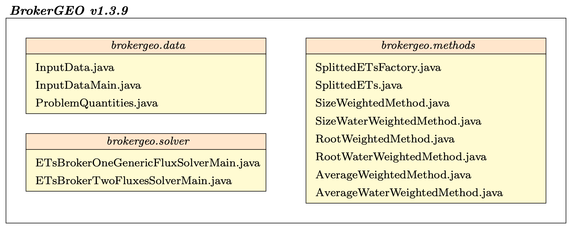
BrokerGEO is an independent OMS3 component used in GEOSPACE-1D to connect WHETGEO-1D to the four different evapotranspiration models of GEOET. The BrokerGEO 1.3.9 version is mainly composed of three packages shown in Fig. 8:

• brokergeo.data

• brokergeo.solver

• brokergeo.methods

The brokergeo.data package assumes the role of overseeing the input data and variables associated with the models. It leverages two classes, namely ProblemQuantities and InputData for input management. These classes are subsequently linked to the classes responsible for computing the partitioned evapotranspiration within each control volume, which are within the brokergeo.solver package. The solver packages contains classes that are designed to invoke methods from the classes in brokergeo.methods, enabling the computation of solutions.

Figure 8 IT software structure of BrokerGEO v1.3.9: packages and classes.

In the UML diagram depicted in Fig. 9, the package comprises two key solver classes: firstly, ETsBrokerOneGenericFluxSolverMain, which is tailored for computing only the split evapotranspiration (ETs). This approach aligns with the prevalent practices in evapotranspiration modeling literature, where most models estimate the comprehensive evapotranspirative flux, encompassing both vegetation transpiration and bare soil evaporation. However, models like Prospero and TranspirationBudget are dedicated exclusively to transpiration computation. Secondly, ETsBrokerTwoFluxesSolverMain is specifically designed to calculate the split transpiration (E_l) and split soil evaporation (E_s) as distinct components.

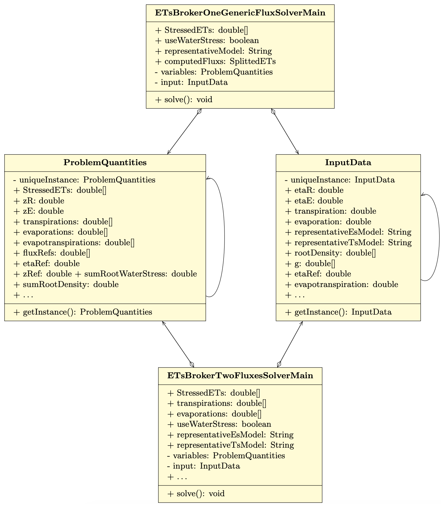
Figure 9 UML class diagram for the ETsBrokerOneGenericFluxSolverMain class and ETsBrokerTwoFluxesSolverMain class. The classes compute the split evapotranspiration directly by calling the methods of the concrete classes through the simple factory pattern shown in Fig. 10. The graph points out the relation of “aggregation” and “association” between the solver classes and the ProblemQuantiites and InputData classes.

Upon a more detailed examination of Fig. 9, it becomes apparent that the connection between the solver classes, specifically ETsBrokerOneGenericFluxSolverMain and ETsBrokerTwoFluxesSolverMain, and the two classes ProblemQuantities and InputData can be characterized as a hybrid of both “association” and “aggregation”.

At the bottom of the programming chain, three classes are responsible for implementing the three equations (Eqs. 16, 17, 18): AverageWaterWeightedMethod.java, SizeWaterWeightedMethod.java, and RootWaterWeightedMethod.java. Any other possible partition formula can be implemented as well by simply adding a class in the method package.

6.2 BrokerGEO factory pattern

Given that multiple methods for partitioning evapotranspiration (ET) can be employed, with the potential for the introduction of new methods in the future, the most adaptable design choice for the IT architecture of BrokerGEO was the simple factory pattern (Gamma et al., 1995).

As shown in Fig. 10, the SplitterETs class is the abstract class, and it contains only the abstract method computeStressedETs. Therefore, we have six possible alternatives that implement a concrete method to compute the split flux:

• AverageWaterWeightedMethod,

• AverageWeightedMethod,

• RootWaterWeightedMethod,

• RootWeightedMethod,

• SizeWaterWeightedMethod,

• SizeWeightedMethod.

The connection between the SplitterETsFactory class and the SplitterETs class is established through the createEvapoTranspirations method. This method enables the factory to produce instances of SplitterETs and its subclasses based on the type string that the user may specify as input to choose which model to use, and the corresponding method is returned.

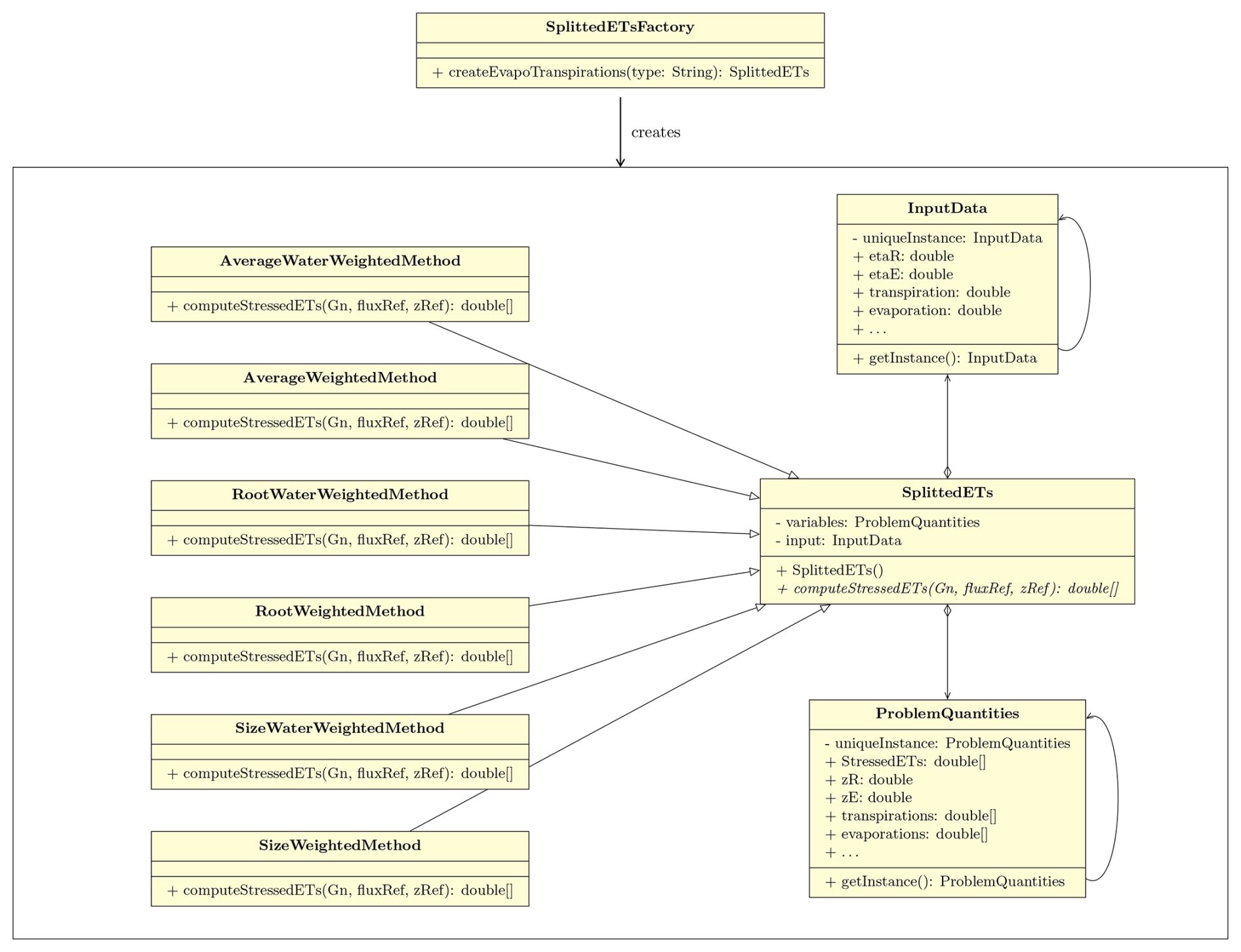
Figure 10 UML class diagram for the Java simple factory applied for the choice of the splitter evapotranspiration method. The SplittedETs class defines the interface that is implemented by the concrete classes AverageWaterWeightedMethod, AverageWeightedMethod, RootWaterWeightedMethod, RootWeightedMethod, SizeWaterWeightedMethod, and SizeWeightedMethod. The UML graph points out the relation of “aggregation” and “association” between the abstract class SplittedETs and the ProblemQuantiites and InputData classes.

Since BrokerGEO operates as an autonomous OMS3 component, all the implemented numerical methods are capable of partitioning a reference flux. This reference flux may represent simple evaporation, transpiration, or the entire evapotranspiration flux.

7 Unveiling GEOSPACE-1D capabilities on practical applications

To demonstrate the capabilities of the model, we present two “virtual” simulations: the first is called the “baseline simulation” (BSL), which simulates the coupled dynamics of infiltration and evapotranspiration, while the second one focuses only on the infiltration process. The simulations are not intended to investigate a particular experimental setup, which would require a longer paper and is an open a topic better addressed in dedicated research. Instead, these simulations serve as a proof of concept, demonstrating that the system functions correctly without integration errors across all tested conditions. This represents only a small subset of the comprehensive simulations performed by the authors to evaluate GEOSPACE's robustness. Water budget closure was verified for all simulations, with supporting documentation provided in the Supplement. All the simulations are readily available in the Supplement, which contains a series of Jupyter notebooks that allow re-executing them and inspecting their results more deeply.

The BSL simulation was done by forcing the model with the input data of the 2-month dataset from the “Spike II” experiment, whose forcings are shown in Fig. 11. A comprehensive description of the experiment is reported in Queloz et al. (2015), Benettin et al. (2019, 2021a, b), and Nehemy et al. (2021).

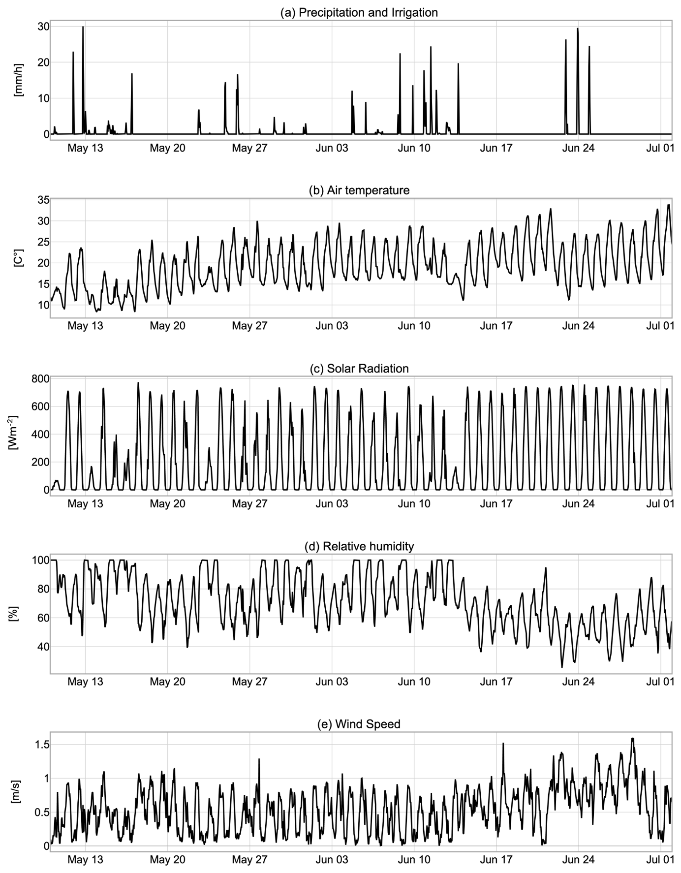
Figure 11 Time series of the dataset from the “Spike II” experiment provided by the meteorological station (MeteoMADD, MADD Technologies Sàrl, Switzerland). The data have been accurately aggregated on an hourly scale to be used as input for the simulation with the GEOSPACE-1D model.

The “Spike II” BSL can be described as a one-dimensional simulation of a homogeneous column of soil of 2.5 m depth with a plant of height of 3.5 m, i.e., a willow. The soil column was discretized with a uniform grid space of 250 control volumes, and we carried out an hourly time step simulation. The soil hydraulic properties are described with the Van Genuchten model (Table 2), and most of them are taken from the work of Asadollahi et al. (2022). The initial condition is assumed to be hydrostatic with ψ=0 m at the bottom. The surface boundary condition is the rainfall and irrigation shown in Fig. 11a. WHETGEO-1D (Tubini and Rigon, 2022) includes a surface water coupled model, which allows the formation of surface ponding, so the surface boundary condition may change from the Dirichlet type – prescribed water suction – to the Neumann type – prescribed flux – and vice-versa, according to the occurring process. At the bottom of the column, we prescribed a free drainage boundary condition with a gravity-driven transient.

Table 1 Summary of the main settings for the baseline simulation: this table presents key parameters and configurations utilized in the baseline simulation.

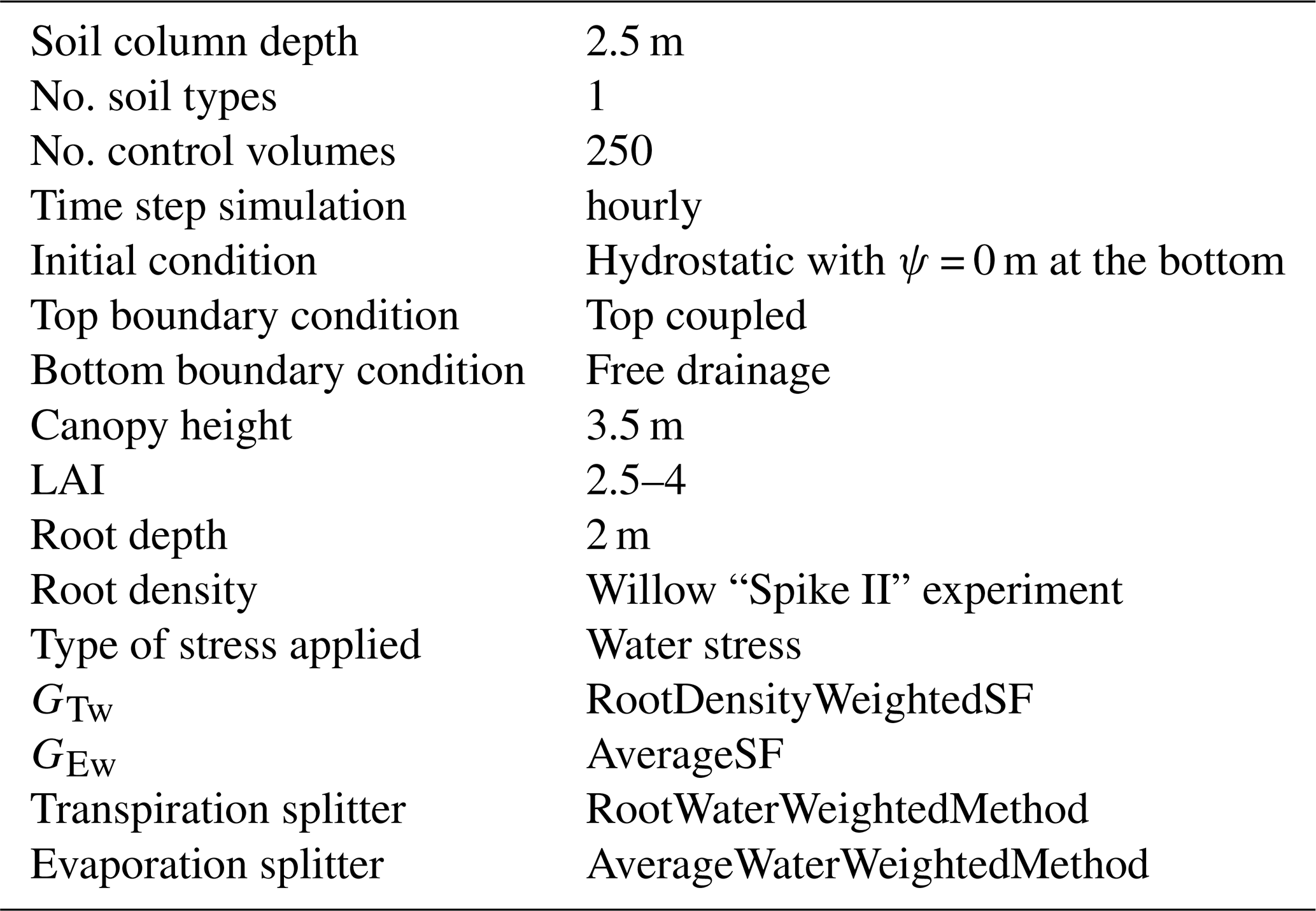
Table 2 Hydraulic properties of the soil column for the baseline simulation.

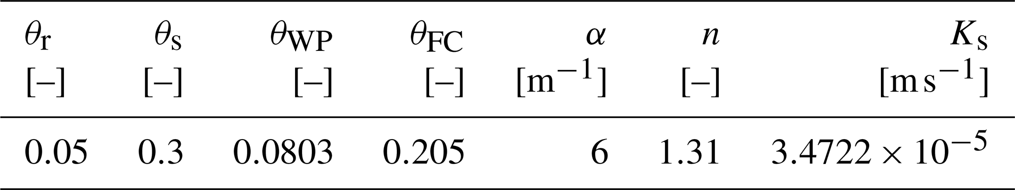
For the evapotranspiration model, we utilized the GEOET–Prospero model, driven by the input data shown in Fig. 11. Our analysis focused on a plant of height of 3.5 m, with leaf area index (LAI) linearly varying from 2.5 to 4 m at the beginning and end of the simulation, respectively. As root depth and density parameters we used the “Spike II” experiment measurements of the willow, and they were kept constant throughout the simulation. Finally, among the Jarvis stresses only the water stress is considered, excluding all environmental stresses, and the representative water stress factor for transpiration G_Tw is computed with the root-density-weighted method. The representative water stress factor for evaporation G_Ew is calculated as the arithmetic mean of the stress values characterizing the depth of the evaporation layer, located 0.2 m from the soil surface. The partitioning of evaporation and transpiration between the control volumes is done by BrokerGEO using AverageWaterWeightedMethod for evaporation and RootWaterWeightedMethod for transpiration.

Table 1 provides a comprehensive overview of the settings employed in the baseline simulation. For further details, please refer to the dedicated folder available on the Zenodo repository (D'Amato and Rigon, 2024) and the original thesis (D'Amato, 2024).

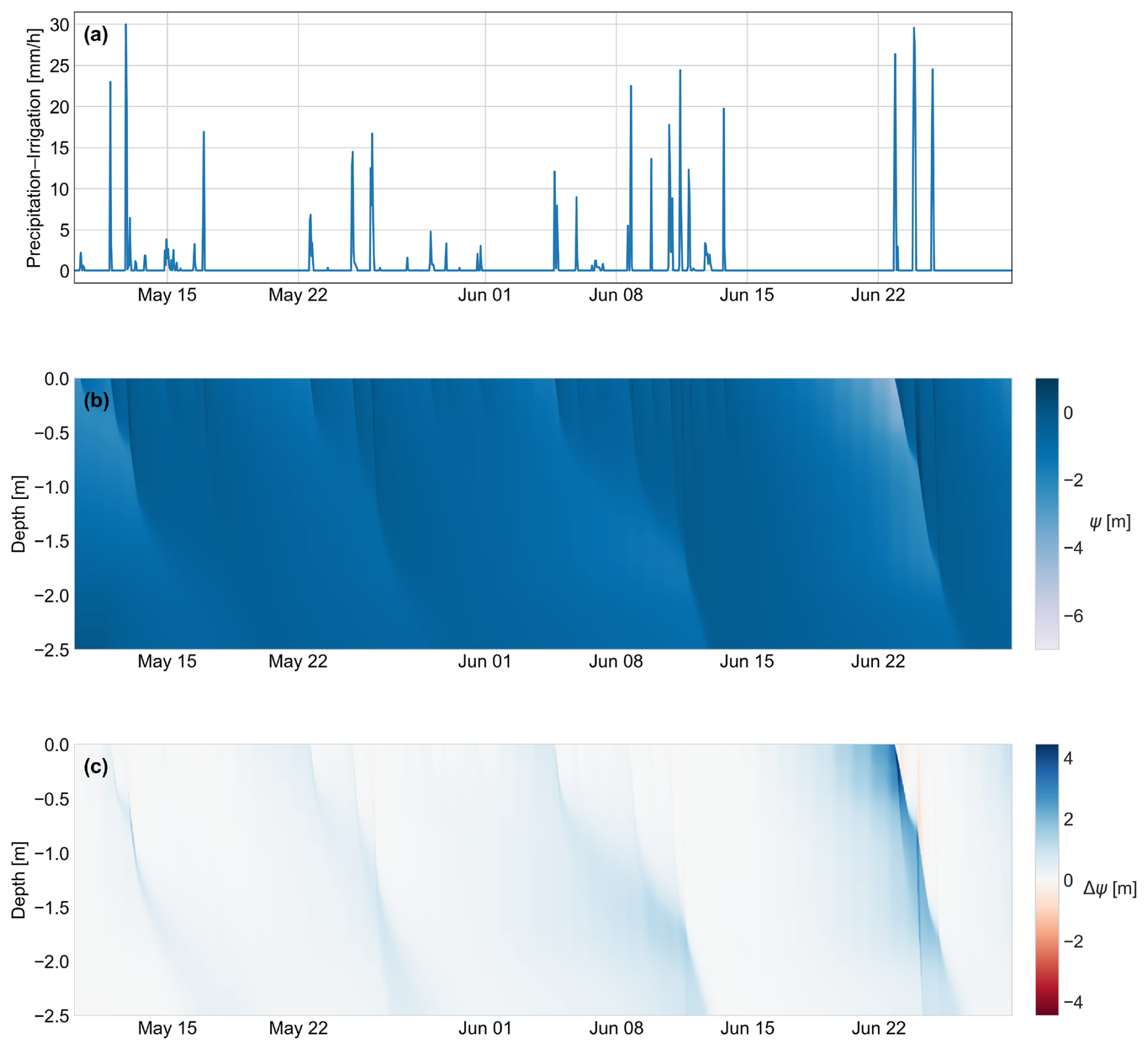
Figure 12 Comparison of soil water potential evolution under scenarios with and without evapotranspiration: panel (a) shows the precipitation–irrigation input over time. Panel (b) depicts the soil water potential (ψ) in the baseline simulation, which includes both infiltration and evapotranspiration. The plot displays depth in meters, with a color scale representing ψ. The darker blue colors indicate increases in ψ resulting from rainfall events and their subsequent propagation over time, typically in a downward direction. As depth increases and water potential decreases, infiltration rates slow down due to reduced soil hydraulic conductivity. This phenomenon is visually represented by the decreasing intensity of the darker signatures and their rightward curvature with depth. Panel (c) illustrates the temporal evolution of the soil water potential difference, defined as $\mathrm{\Delta }\mathit{\psi }={\mathit{\psi }}_{\text{R}}-{\mathit{\psi }}_{\text{BSL}}$, where ψ_R refers to the simulation with infiltration only and ψ_BSL to the baseline simulation. A diverging color map centered at zero is used to represent Δψ values. Positive differences (blue) indicate higher ψ_R in the infiltration-only case, while negative differences (red) indicate lower ψ_R. These deviations primarily result from the absence of evapotranspiration in the infiltration-only simulation.

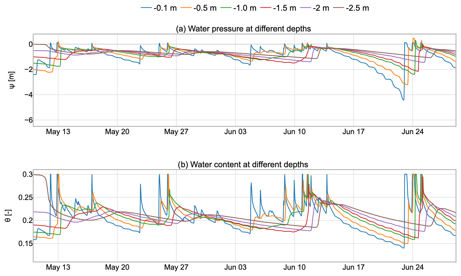
Figure 13 (a) Soil water potential and (b) water content evolution with time at different depths in the baseline simulation. The data in these two figures are clearly related through the soil water retention curve. Notably, following certain rainfall events, soil saturation (ψ>0) is achieved, which is a condition that cannot be adequately handled by solvers less sophisticated than those implemented in GEOSPACE.

Figure 12b depicts the temporal evolution of the soil water potential of the BSL simulation following the rainfall event illustrated in Fig. 12a. Darker blue patterns indicate higher soil water potential, demonstrating a noticeable increase following irrigation or rainfall episodes. In the last events, saturation occurs, leading to surface ponding, eventually resulting in the formation of an infiltrating saturated front. The above situation is better clarified in Fig. 13 where saturation is clearly generated at the surface (blue line) and quickly propagates in the soil down to −1.5 m.

No instabilities along the simulation are visible, even when the systems move from unsaturated to saturated conditions and vice versa, and the mass balance closure is verified, with the error in the closure being around 10⁻⁹ m as shown in the Supplement.

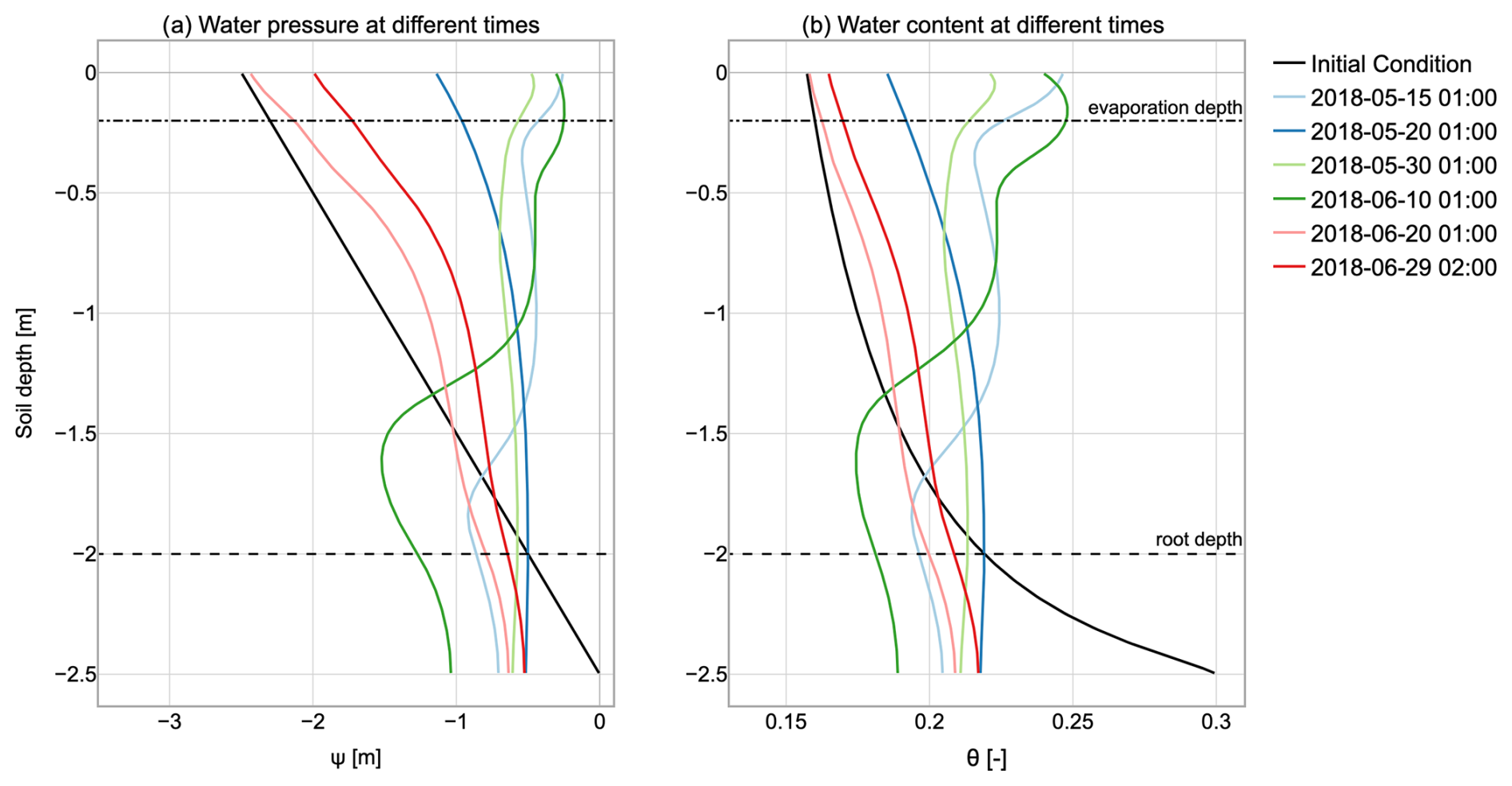
Figure 14 (a) Evolution of soil water potential and (b) water content along the soil profile at various arbitrarily chosen times in the baseline simulation. The initial condition (depicted in black) is hydrostatic but evolves rapidly upon commencement of rainfall. The resulting evolution exhibits a distinct vertical pattern corresponding to the root distribution profile. At the lower portion of the profile, the final conditions are notably influenced by the free drainage boundary condition imposed at the bottom.

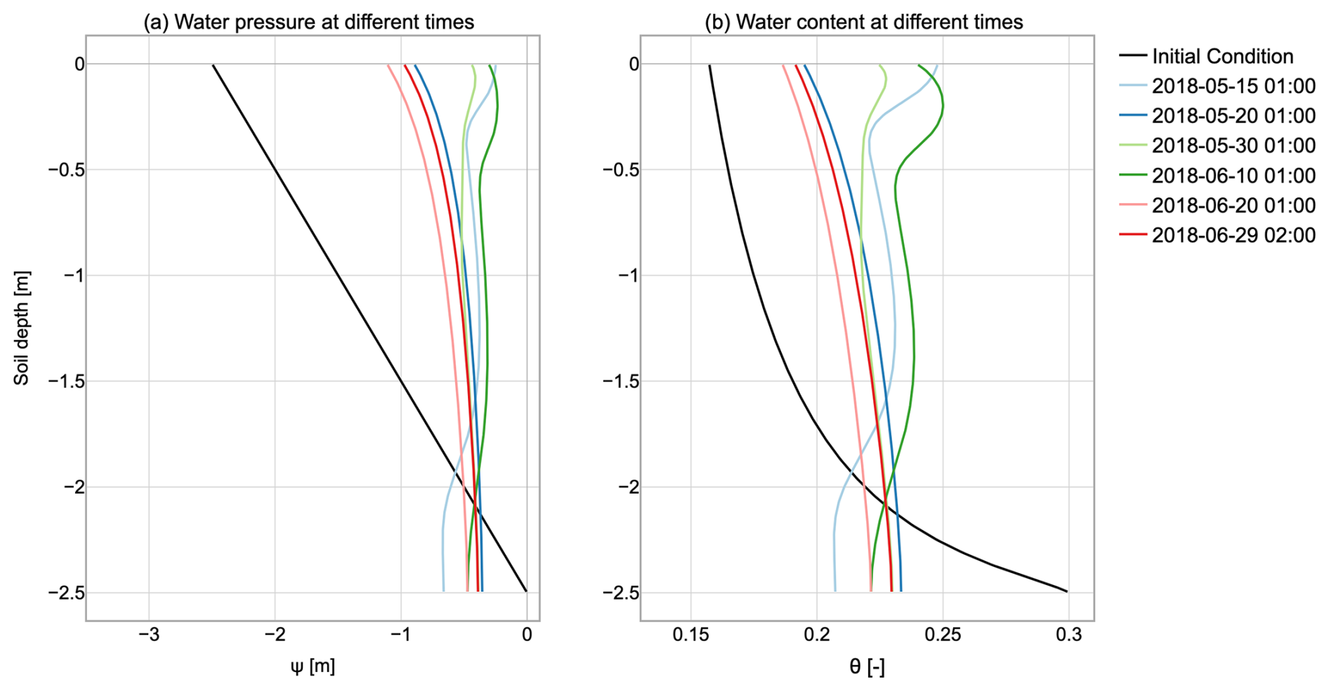
Figure 15 (a) Evolution of soil water potential and (b) water content along the soil profile at various arbitrarily chosen times in a scenario without evapotranspiration. Under identical initial and lower boundary conditions as in the previous figure, this second simulation logically maintains a higher soil water content throughout the profile.

As depicted in Fig. 14, the GEOSPACE-1D outputs provide the necessary data to visualize water pressure and water content profiles at different time steps. This particular figure represents the scenario estimating the combined effects of infiltration and transpiration on soil moisture.

In the second virtual simulation, we replicated the baseline simulation while excluding the evapotranspiration process, thus following the development of the infiltration process in the soil column without evapotranspiration. The outputs of this simulation are in Figs. 15 and 12c. In particular, Fig. 15 serves as a visual comparison, illustrating the dynamics of infiltration without water extraction by the plant. The increased saturation of the soil column compared to the baseline simulation is particularly evident when comparing Figs. 14 and 15.

For a more comprehensive analysis, Fig. 12c illustrates the temporal evolution of the soil water potential difference along the soil profile, defined as $\mathrm{\Delta }\mathit{\psi }={\mathit{\psi }}_{\text{R}}-{\mathit{\psi }}_{\text{BSL}}$, where ψ_R refers to the simulation with infiltration only and ψ_BSL to the baseline simulation with coupled evapotranspiration. This comparison highlights how the exclusion of evapotranspiration processes significantly alters soil water dynamics. In particular, the absence of evapotranspiration results in higher soil water potentials over time, especially in the upper layers, where root water uptake and evaporation typically occur more intensively. These differences are amplified with increasing time elapsed since the last precipitation event, creating a cumulative divergence in the soil moisture profile. This divergence becomes less pronounced following new precipitation inputs, which temporarily reduce the evapotranspiration-induced differences by replenishing soil moisture across all simulation scenarios.

Although a comprehensive analysis of real-world cases exceeds the scope of this paper, our results clearly challenge the conventional “business as usual” simulation approach that estimates infiltration without adequately accounting for plant water uptake. The total bottom flux without evapotranspiration amounts to 602.31 mm, a stark contrast to the 180.09 mm observed in the baseline simulation, resulting in a 234.6 % increase in groundwater recharge.

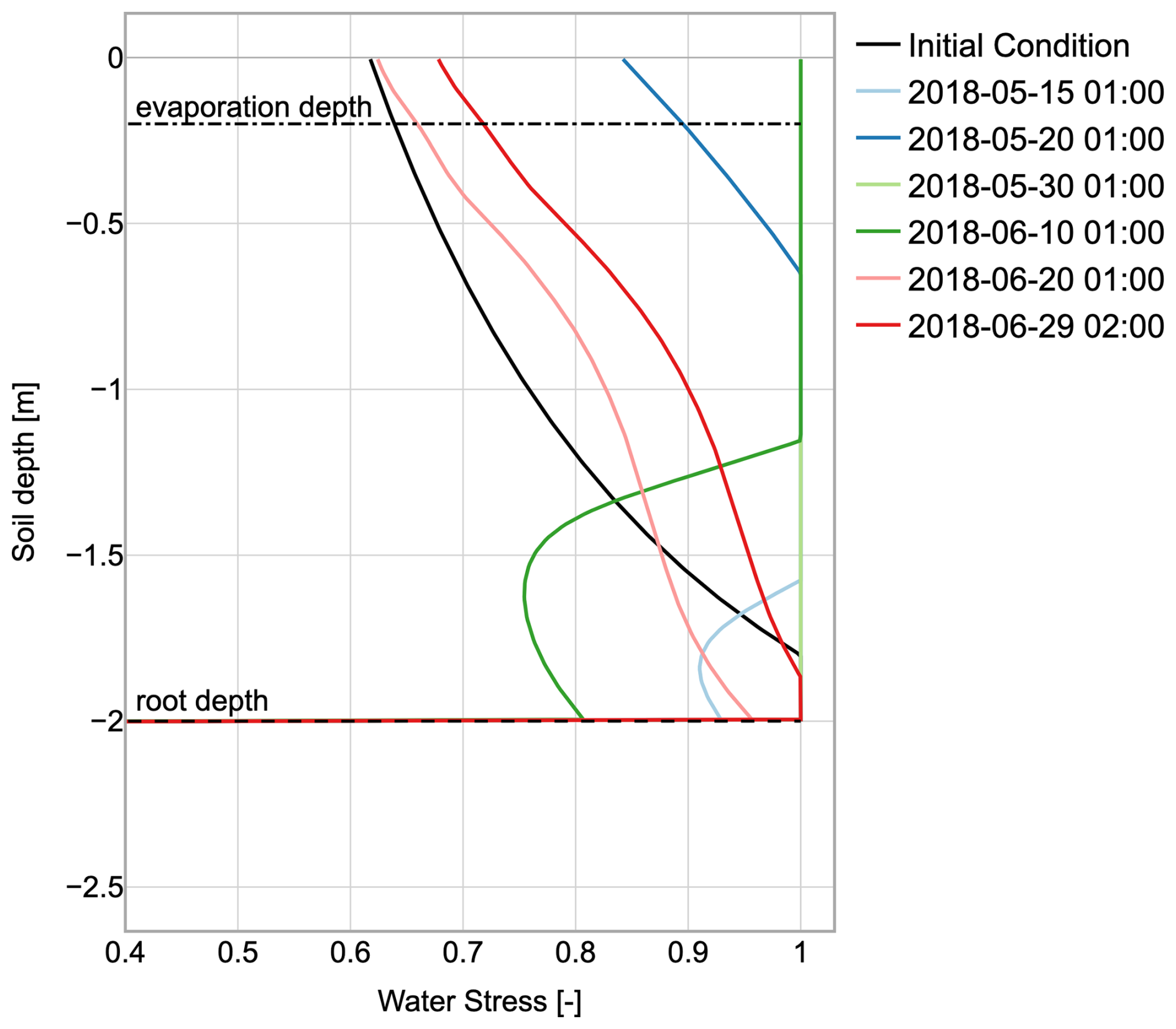
Figure 16 Evolution of the water stress factor along the soil profile at various arbitrarily chosen times in the baseline simulation. This information can support more accurate and efficient irrigation scheduling based on soil water availability.

Figure 16 represents the evolution of the water stress in time and depth in the BSL. As said before, the root depth is considered constant in time but a time series describing the root depth growth could be provided as an input to the model, if available. The bulk stress factor can be easily estimated from the data provided and is shown in the Zenodo folder material (D'Amato and Rigon, 2024). Unlike conventional modeling practices where irrigation is triggered based on soil water content or soil water potential measurements, GEOSPACE enables direct assessment of water stress levels at any soil depth. However, it is important to note that the current version of the software does not yet incorporate the phenomenon of hydraulic redistribution, whereby roots can redistribute water vertically through the soil profile.

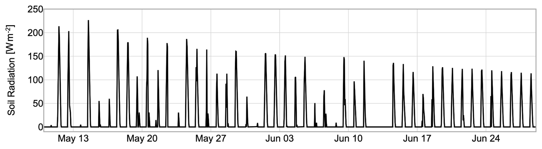
Figure 17 Radiation reaching the ground, given the prescribed LAI as input, in the baseline simulation. The decrease in radiation depends on meteorological conditions and the increase in LAI with time.

Solar radiation is measured in this experiment, but it undergoes filtration as it passes through the plant canopy, as described by the model presented in the Supplement. The remaining radiation, known as residual radiation, is depicted in Fig. 17, and it reaches the soil, where it is utilized to estimate soil evaporation using the PM-FAO model. The estimated soil evaporation and transpiration rates are then shown in Fig. 18.

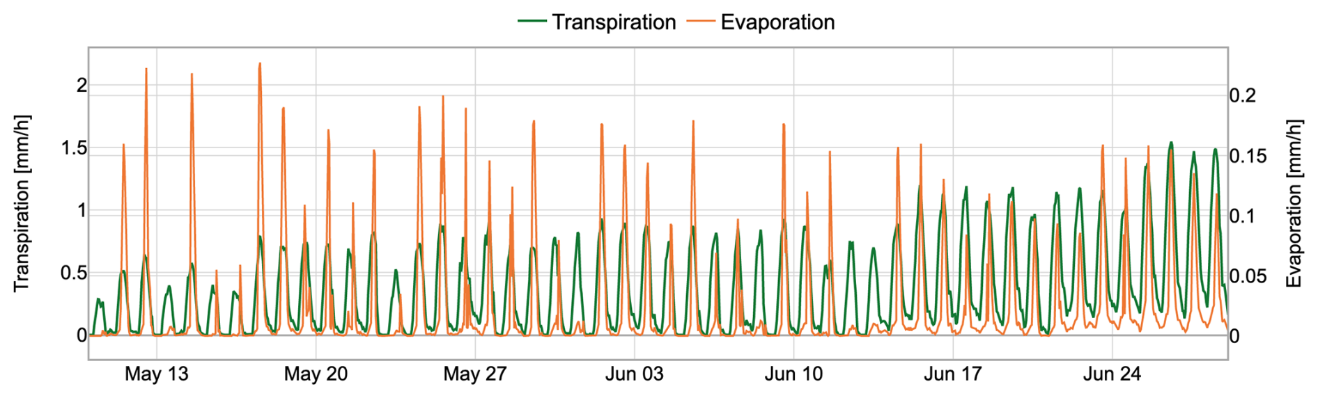
Figure 18 Evolution of transpiration (green) and evaporation (orange) fluxes with time in the baseline simulation. The observed increase in transpiration over time results from the concurrent increases in solar radiation approaching the summer solstice, vegetation leaf area index (LAI), and root system expansion.

User information: input and output

The GEOSPACE-1D system exhibits a modular structure, necessitating various inputs contingent upon the specific modules employed. Table 3 summarizes the general inputs required for all components in GEOSPACE-1D. These simulation parameters, including the simulation's temporal parameters, are user-defined in the OMS3 .sim file.

In the context of WHETGEO, input data can be categorized into two main key components: time series and computational grid data (Table 4). Time series data primarily serve to define the boundary conditions for the case study. These time series are encapsulated within .csv files specific for OMS3 format. Computational grid data encompass domain discretization, initial conditions, and terrain parameters, all stored in Network Common Data Form (NetCDF) files. The processing of time series and computational grid data is executed using specialized Python modules integrated into the geoframepy package (Tubini and Rigon, 2021).

Specifically, the time series data for boundary conditions need meteorological information about precipitation, the presence of surface ponding, and the hydraulic condition at the base of the soil column. When addressing computational grid considerations, it is essential to specify the structure of the soil column, such as the soil horizons and hydrological/hydraulic parameters, or to employ literature data for saturated hydraulic conductivity, water content at saturation, residual values, and the water retention curve parameters (SWRC), as outlined in WHETGEO (Tubini, 2021). Most of these soil parameters, implemented as default in WHETGEO, are available in Bonan (2019), but any other dataset can be used as well by changing the appropriate configuration files.

The input data required by GEOET are time series of meteorological forcings that could be downloaded from online weather service portals. Specifically, the input data include time series of air temperature, wind speed, relative humidity, solar radiation, and pressure, but they depend on the evapotranspiration model used from those available (Table 5). In the context of vegetation characterization, leaf area index data and canopy height, acquired from the literature or satellite sources, are fundamental for the computation of transpiration flux. Root depth (z_R) and density (δ_R) have to be specified in the creation of computational grid data because their information is needed in each control volume. Additionally, parameters associated with stress factor calculations, such as the water content at wilting point (θ_WP) and field capacity (θ_FC), can be readily sourced from available literature. Finally, the user has to specify which model to use to compute the representative water stress factor G_w (Sect. 5) and, accordingly, also the model to split evapotranspiration with BrokerGEO (Table 6) as described in Sect. 6.2. The output data of GEOSPACE-1D depend on the model combination that we use. Table 7 summarizes the GEOSPACE-1D outputs.

The WHETGEO model generates output data in NetCDF format. Nevertheless, these outputs (as well as the inputs) are managed separately by specifically designed OMS3 components, which handle the writing and reading processes. This separation ensures modularity and flexibility, allowing alternative writers and readers to be provided to adapt to different file formats as required.

For ease of reading, we provide users with extensively commented Python notebooks, through which all possible outputs of WHETGEO-1D can be accessed. Outputs include water suction [m], water content [–], Darcy velocity [m s⁻¹], mass balance error, and others. If the heat transport model is used, the soil temperature is also outputted.

To date, GEOET results have been stored in OMS3 CSV files, and the type of output depends on the evapotranspiration model used in GEOSPACE-1D, as highlighted in Table 7. Specifically, if we consider Prospero for transpiration and Penman–Monteith for soil evaporation, the estimated output quantities are soil evaporation [L T⁻¹], transpiration [mm T⁻¹], latent and sensible heat flux [W m⁻²], leaf temperature [°C], water vapor deficit [–], and so on. For a complete description, please refer to the Jupyter notebook 00_Notebook of GEOSPACE-1D on the GitHub page (https://github.com/GEOframeOMSProjects/OMS_Project_GEOSPACE-1D, last access: 1 October 2025).

It is important to highlight that a common challenge in conducting simulations is the scarcity of data required to perform them. For instance, obtaining data on root density can be difficult, and it is not always guaranteed that a study site will have a meteorological station providing all the necessary data outlined in Tables 4 and 5. This is why GEOET offers both simple and complex evapotranspiration models. In cases where all the required data for complex models are not available, simpler models requiring fewer inputs can be utilized.

Taking Prospero again as an example, it is possible to encounter situations where only a few of the necessary inputs are missing. In such instances, default data from the model or data from existing literature can be used. In the context of evapotranspiration models, radiation is a critical input that must never be absent, as it serves as the primary driver. Similarly, when it comes to roots, while the depth of roots may be known, their density is often unknown. In such cases, one may opt for an arbitrary distribution or reconstruct it using data from the literature, or more users can use one of the root density growth methods implemented in GEOET. For more information please refer to D'Amato (2024).

Table 3 General inputs required for all components in GEOSPACE-1D. These simulation parameters, including the simulation's temporal parameters, are user-defined in the OMS3 .sim file.

Table 4 Input data for WHETGEO component, categorized into two main elements: time series and computational grid data.

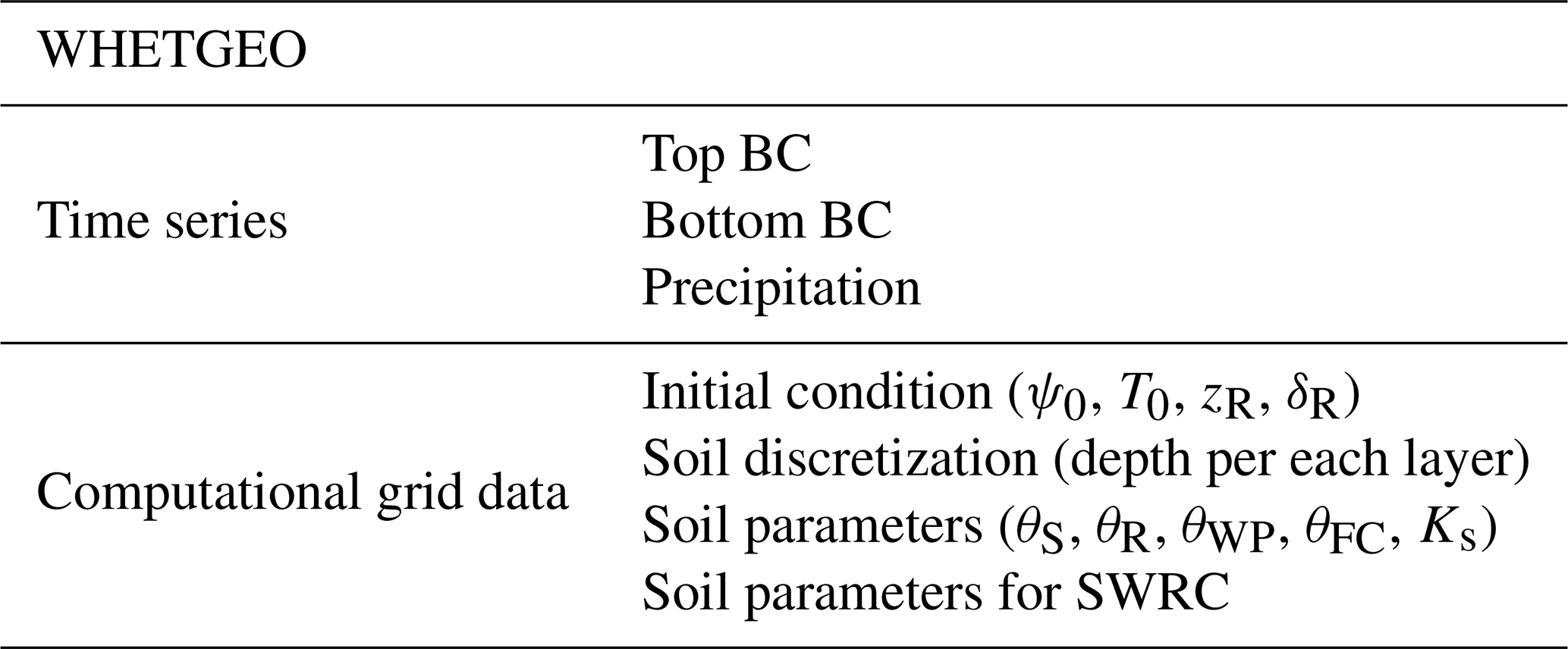
Table 5 Time series input data for GEOET component and a comparison of input requirements for different evapotranspiration models (Prospero, PM-FAO, and PT) in GEOET.

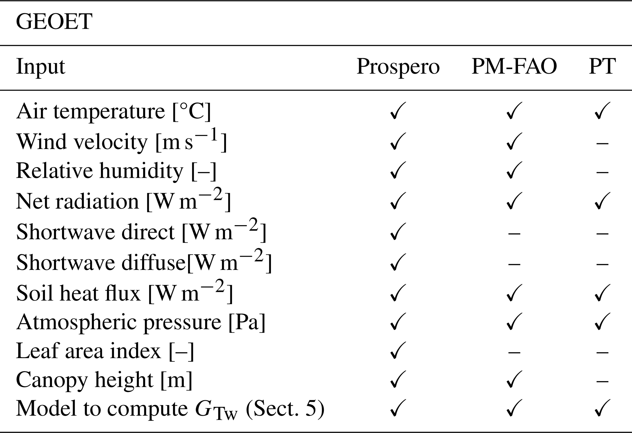
Table 6 Overview of key inputs within the BrokerGEO model: the algorithm for computing reference evapotranspiration (ET_ref,i) and details about the computational grid and the reference flux (evaporation, transpiration, or evapotranspiration) to be split.

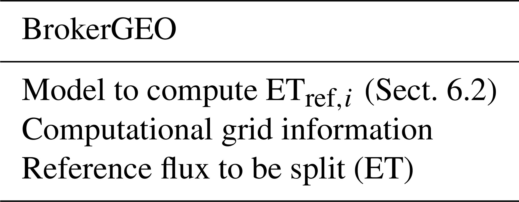
Table 7 GEOSPACE-1D model outputs: hydrological and meteorological variables between WHETGEO output (NetCDF) and GEOET output (.csv).

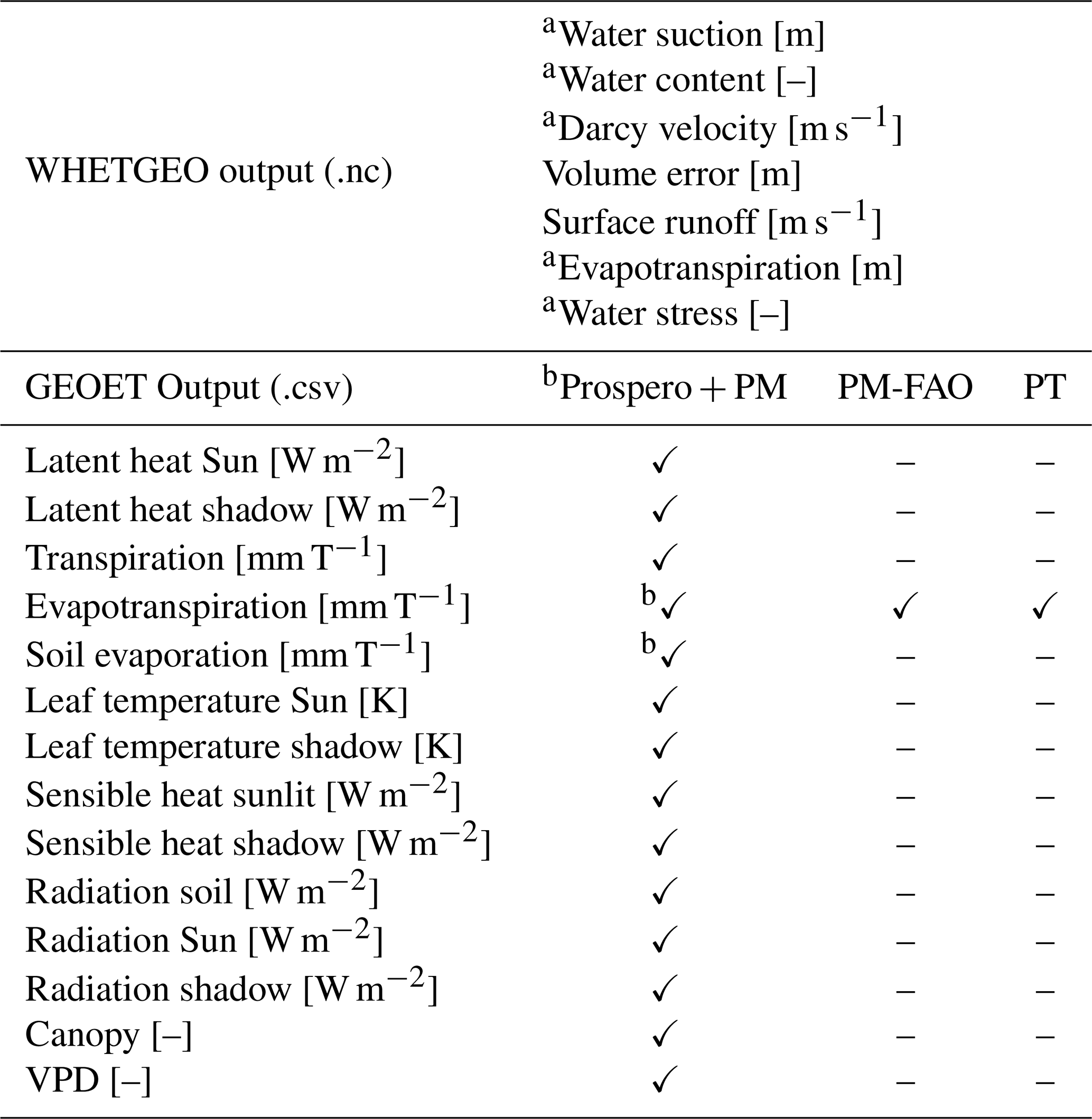
^a This variable includes all outputs at the current time step for each control volume. ^b When using Prospero, soil evaporation is computed with the PM model, setting a predefined evaporation depth as input.

8 User information: code availability

The latest executable code of the WHETGEO model with the new classes mentioned before can be downloaded from https://github.com/geoframecomponents/WHETGEO-1D (last access: 1 October 2025) and can be compiled by following the instructions therein. The version of the OMS3 compiled project can be found at https://github.com/GEOframeOMSProjects/OMS_Project_WHETGEO1D (last access: 1 October 2025).

The Object Modeling System v.3 (OMS3) is a component-based environmental modeling framework introduced by David et al. (2013). More information is in the Supplement.

While the majority of the content presented thus far holds broad relevance, it is important to note that the deployment example showcased here pertains to a one-dimensional (1D) context. Comprehensive information on GEOSPACE-1D, intended for both users and developers, can be found in the Supplement. Included within it is a Jupyter notebook labeled with the prefix “00_”, affectionately referred to as “Notebook Zero”, which serves as a comprehensive guide for executing the code pertaining to any of the components. The latest executable code can be downloaded from https://github.com/geoframecomponents/GEOSPACE-1D (last access: 1 October 2025) and can be compiled by following the instructions therein. Finally, the version of the OMS3 compiled project can be found at https://github.com/GEOframeOMSProjects/OMS_Project_GEOSPACE-1D.

The code can be executed in the OMS3 console, which can be downloaded and installed according to the instructions given at https://geoframe.blogspot.com/2020/01/the-winter-school-on-geoframe-system-is.html (last access: 1 October 2025).

The various components of GEOSPACE v.1.2.9 are finally compiled and grouped in the following .jar files:

• whetgeo1d-1.2.9 includes the WHETGEO model components;

• brokergeo-1.3.9 includes the BrokerGEO coupler;

• geoet-1.5.9 includes the GEOET model containing the ET modules, besides the root functioning, the modules that split the radiation into the canopy and soil layers, and the stress factor estimators;

• buffer-1.1.9 contains ancillary modules for the management of data in memory and their eventual printing;

• closureequation-1.1.9 manages the equations that are actually solved in WHETGEO;

• netcdf-1.1.9 manages the input and output from and to NetCDF files;

• numerical-1.0.2 contains the core algorithms for the solutions of the equations.

The integration of all components took place within the Object Modeling System v3 framework (OMS3) and interlinked within GEOSPACE. Notably, within the aforementioned components, specific to WHETGEO, are modules such as buffer, closureequation, netcdf, and numerical. For comprehensive information on these WHETGEO-specific components, you can refer to Tubini (2021). Due to the modularity of the system, whilst the components were developed and can be enhanced independently, they can be seamlessly used at runtime by connecting them with the OMS3 DSL based on Groovy. OMS3 provides the basic services and, among them, tools for calibration and implicit parallelization of component runs.

Finally, more comprehensive information about GEOframe is available at the following.

• https://abouthydrology.blogspot.com/2015/03/jgrass-newage-essentials.html (last access: 1 October 2025)

• https://geoframe.blogspot.com/2020/01/gsw2020-photos-and-material.html (last access: 1 October 2025)

9 Conclusions

This paper presents and discusses the implementation of the GEOSPACE framework, in particular its one-dimensional development, which stands out among various software programs for its component-based organization leveraging the OMS3 framework. GEOSPACE-1D comprises three main components: WHETGEO, GEOET, and BrokerGEO. WHETGEO serves as a solver for the Richards–Richardson equation, employing a novel integration algorithm, incorporating the soil energy budget, and featuring automatic switching between saturated and unsaturated conditions. GEOET implements various evapotranspiration formulas and the Prospero model, which concurrently solves transpiration and heat transport alongside the stationary energy budget. Additionally, GEOET provides information on the temperature and water pressure differentials between leaves and air. BrokerGEO acts as a connector between the GEOET and WHETGEO solvers, redistributing evaporation and transpiration demands within the soil column. Additionally, the paper delves into the underlying philosophy of the GEOSPACE framework, which can be succinctly summarized as a structure designed to facilitate modifications aimed at exploring soil–plant–atmosphere interactions under various hypotheses and incorporating new research findings. This objective is accomplished by implementing core functionalities as relationships among abstract objects, specifically interfaces, which are subsequently instantiated into concrete classes, allowing flexibility for user/programmer choices. The instantiation mechanism for these classes is achieved using the factory pattern. A consequence of the above choices is that, for instance, the creation of a new method for estimating the water stress consists of just adding a new class that extends the general interface. Adding a new method for estimating transpiration or evaporation can require a few classes, depending on the complexity of the method, but always obeying the prescription that the code remain “open to extensions and closed to modifications”. In the cases already deployed, the Priestley–Taylor formula is implemented by using three classes, while the Prospero model requires a few more as shown in Fig. 6. Departing from the strict object-oriented paradigm, which necessitates the creation and destruction of immutable classes, GEOSPACE-1D adopts a more conventional approach, particularly familiar to scientists, for classes dedicated to data containment. Data classes are structured as singletons, instantiated once and continuously updated with new content at each time step.

The model's capabilities are showcased through a “baseline” simulation, which compares infiltration estimates with and without evaporation and transpiration based on data collected in the “Spike II” experiment at the École Polytechnique Fédérale de Lausanne. The simulations conducted aimed to highlight the functionalities and capabilities of the system, demonstrating its ability to maintain water mass and energy conservation. It is worth noting that during these simulations, the soil column experiences saturation due to a perched water table while transpiration occurs. Throughout the simulations, the mass budget closure is rigorously monitored and consistently achieved with high precision, despite the diverse range of simulated conditions. These simulations exhibit a strong correspondence with measured data, as further elaborated in a companion paper currently in preparation (D'Amato et al., 2025c).

As part of the project, a collection of companion Jupyter notebooks has been developed to elucidate the process of inputting data required by GEOSPACE-1D across various configurations. This aligns with the model's implementation philosophy, which separates the handling of model-agnostic components (written in Python and potentially compatible with other modeling platforms) from the model-specific elements (programmed in Java in our case). The outcome of any simulation setup is encapsulated in OMS3 “.sim” files, facilitating easy sharing. In line with promoting FAIR principles in modeling, all aspects related to GEOSPACE-1D including executables, notebooks, simulations, and input and output data files are consolidated within OMS3 projects and can be readily distributed. Everything utilized in this paper is included in the dedicated folder available on the Zenodo repository (D'Amato and Rigon, 2024) for third-party inspection and self-instruction. Furthermore, the source code is openly accessible and provided on GitHub, as detailed in the relevant sections of the paper. Additionally, instructional videos demonstrating the system's functionality can be found on the GEOframe blog.

Appendix A: GEOET

The evapotranspiration component, GEOET, is a deep refactoring of the GEOframe-ETP model (Bottazzi, 2020; Bottazzi et al., 2021). The GEOET framework incorporates four evapotranspiration models, as illustrated in Fig. 6. Starting with the simplest model, we have the Priestley–Taylor model (PT), the Penman–Monteith FAO (PM) approximation, an adaptation of the Penman–Monteith model, the Prospero model (Bottazzi, 2020; Bottazzi et al., 2021), and the TranspirationBudget model, a complex computation of the energy budget at the canopy scale described in D'Amato and Rigon (2025). The Priestley–Taylor model is already fully described in the main text, while the PM model and the Prospero model require some further explanations.

A1 Penman–Monteith FAO additional information

Chapter 2 of the FAO evapotranspiration book (Food and Agriculture Organization of the United Nations, https://www.fao.org/3/X0490E/x0490e06.htm#TopOfPage, last access: 1 October 2025) introduces the user to the need to standardize one method to compute reference evapotranspiration (ET₀). As described in Bottazzi (2020), the Penman–Monteith FAO is the approximation for the Penman–Monteith equation, defined for a reference crop as a hypothetical crop with an assumed height of 0.12 m, having a surface resistance of 70 s m⁻¹ and an albedo of 0.23. It is widely used, especially in the agricultural field.

Starting from the Penman–Monteith equation, the FAO approximation for a grass reference surface leads to the computation of a reference evapotranspiration as follows:

$$\begin{array}{}\text{(A1)}& {\mathrm{ET}}_{\mathrm{0}}={\displaystyle \frac{\mathrm{1}}{\mathit{\lambda }}}{\displaystyle \frac{\mathrm{0.408}\mathrm{\Delta }(R_{\mathrm{n}}-G)+\mathit{\gamma }\frac{\mathrm{900}}{T+\mathrm{273}}{u}_{\mathrm{2}}(e_{\mathrm{s}}-e_{\mathrm{a}})}{\mathrm{\Delta }+\mathit{\gamma }(\mathrm{1}+\mathrm{0.34}{u}_{\mathrm{2}})}},\end{array}$$

where ET₀ is the reference evapotranspiration [mm d⁻¹], R_n is the net radiation at the crop surface [MJ m⁻² d⁻¹], G is the soil heat flux density [MJ m⁻² d⁻¹], T is the mean daily air temperature at 2 m height [°C], u₂ is the wind speed at 2 m height [m s⁻¹], e_s is the saturation vapor pressure [kPa], e_a is the actual vapor pressure [kPa], (e_s−e_a) is the saturation vapor pressure deficit [kPa], and D is the slope vapor pressure curve [kPa °C⁻¹],

Using the latent heat constant λ, the reference evapotranspiration can be converted to the reference latent heat:

$$\begin{array}{}\text{(A2)}& E_{\mathrm{0}}={\mathrm{ET}}_{\mathrm{0}}\cdot \mathit{\lambda }.\end{array}$$

FAO computes the actual evapotranspiration using the water stress coefficient K_s and the single crop coefficient K_c:

$$\begin{array}{}\text{(A3)}& E_{\mathrm{FAO}}={\mathrm{ET}}_{\mathrm{0}}\cdot K_{\mathrm{s}}\cdot K_{\mathrm{c}}.\end{array}$$

Values for K_c are given by the FAO in Table 12 of Chap. 6 (https://www.fao.org/3/X0490E/x0490e0b.htm#TopOfPage:~:text=TABLE%2012.%20Single%20(time%2Daveraged)%20crop%20coefficients%2C%20Kc%2C%20and%20mean%20maximum%20plant%20heights%20for%20non%20stressed%2C%20well%2Dmanaged%20crops%20in%20subhumid%20climates%20(RHmin%20%C2%BB%2045%25%2C%20u2%20%C2%BB%202%20m/s)%20for%20use%20with%20the%20FAO%20Penman%2DMonteith%20ETo, last access: 1 October 2025). The water stress coefficient K_s can by computed as

$$\begin{array}{}\text{(A4)}& {\displaystyle }{K}_{\mathrm{s}}={\displaystyle \frac{\mathrm{TAW}-D_{\mathrm{r}}}{\mathrm{TAW}-\mathrm{RAW}}}={\displaystyle \frac{\mathrm{TAW}-D_{\mathrm{r}}}{(\mathrm{1}-p)\mathrm{TAW}}},\text{(A5)}& {\displaystyle }\mathrm{RAW}=p\cdot \mathrm{TAW},\text{(A6)}& {\displaystyle }\mathrm{TAW}=\mathrm{1000}({\mathit{\theta }}_{\mathrm{FC}}-{\mathit{\theta }}_{\mathrm{WP}})\cdot Z_{\mathrm{r}},\text{(A7)}& {\displaystyle }\mathrm{TAW}=\mathrm{1000}({\mathit{\theta }}_{\mathrm{FC}}-\mathit{\theta })\cdot Z_{\mathrm{r}},\end{array}$$

where K_s is a dimensionless transpiration reduction factor dependent on available soil water [0–1], D_r is root zone depletion [mm], TAW is total available soil water in the root zone [mm], p is the fraction of TAW that a crop can extract from the root zone without suffering water stress [–], θ_FC is the water content at field capacity [m³ m⁻³], θ_WP is the water content at wilting point [m³ m⁻³], θ_WP is the measured water content [m³ m⁻³], and Z_r is the rooting depth [m].

A2 Prospero model

The Prospero model (Bottazzi, 2020) (Bottazzi et al., 2021) is a physically based approach for calculating canopy transpiration (T) and soil evaporation E. These processes are considered for both sunlit and shaded fractions of the canopy. E from the soil is determined according the FAO Penman–Monteith model; meanwhile, T is computed using a modified version of the Schymanski and Or (Schymanski and Or, 2017) (SO) model, which has been upscaled to address canopy-level transpiration and modified to ensure mass conservation during periods of water stress. The SO model solves the stationary energy budget coupled with the water vapor transport Dalton equation and the sensible heat S equation by using a suitable simplification of the Clausius–Clapeyron formula.

For a more in-depth exploration of this topic, readers are encouraged to refer to the comprehensive information provided in Bottazzi (2020) and D'Amato and Rigon (2025).

To expand the applicability of this equation to the canopy, Bottazzi (2020) chose to implement a two-big-leaf approach (Dai et al., 2004; Luo et al., 2018), utilizing the Sun/shade model introduced by De Pury and Farquhar (1997) and illustrated in the Supplement. This approach enables the calculation of the fraction of the canopy exposed to direct sunlit and the fraction in shade, along with the radiation absorbed by various canopy layers. Specifically, Prospero employs this two-leaf Sun–shade approach, while treating the soil as an additional layer. Other environmental variables such as air temperature, relative humidity, wind, and longwave radiation are assumed to remain constant within the canopy, allowing it to be treated as a single large leaf emitting latent heat proportionate to its area and shortwave radiation.

The SO approach overcomes several limitations of the Penman–Monteith equation, particularly in its representation of transpiring leaf area and leaf thermal capacity, along with their feedback on the energy balance. Incorrectly representing the transpiring leaf area can significantly impact the overall energy balance. Consequently, the energy budget can be reformulated in terms of the area capable of exchanging fluxes and the equilibrium leaf temperature as follows:

$$\begin{array}{}\text{(A8)}& R_{\mathrm{s}}=a_{\mathrm{sH}}{A}_{\mathrm{tr}}{R}_{\mathrm{ll}}\left(T_{\mathrm{l}}\right)+a_{\mathrm{sE}}{A}_{\mathrm{tr}}{E}_{\mathrm{l}}\left(T_{\mathrm{l}}\right)+a_{\mathrm{sH}}{A}_{\mathrm{tr}}{H}_{\mathrm{l}}\left(T_{\mathrm{l}}\right),\end{array}$$

where a_sH is the side of the surface exchanging sensible heat (1 for soil, 2 for leaves) [–], a_sE is the side of the surface exchanging latent heat (1 for amphistomatous leaves) [–], A_tr is the area exchanging fluxes (radiation, sensible, and latent heat) [m² m⁻²], and T_l is the equilibrium leaf temperature [K].

The longwave radiation is computed as

$$\begin{array}{}\text{(A9)}& R_{\mathrm{ll}}=a_{\mathrm{sH}}{A}_{\mathrm{tr}}{\mathit{ϵ}}_{\mathrm{l}}\mathit{\sigma }(T_{\mathrm{l}}^{\mathrm{4}}-T_{\mathrm{a}}^{\mathrm{4}}),\end{array}$$

and T is computed as

$$\begin{array}{}\text{(A10)}& E_{\mathrm{l}}=c_{\mathrm{E}}(a_{\mathrm{sE}},A_{\mathrm{tr}})\cdot \left[\mathrm{\Delta }\right(T_{\mathrm{l}}-T_{\mathrm{a}})+P_{\mathrm{ws}}-P_{\mathrm{w}}].\end{array}$$

The sensible heat is computed as

$$\begin{array}{}\text{(A11)}& H_{\mathrm{l}}=c_{\mathrm{H}}(a_{\mathrm{sH}},A_{\mathrm{tr}})\cdot \left[\right(T_{\mathrm{l}}-T_{\mathrm{a}}\left)\right].\end{array}$$

A_tr is the transpiring surface for a unit of ground surface [–], a_sE represents the sides of the surface exchanging latent heat (equal to 1 for hypostomatous, 2 for amphistomatous [–]), a_sH represents the sides of the surface exchanging sensible heat and longwave radiation (equal to 1 for soil, 2 for leaves [–]), and P_ws and P_w are the saturation water vapor pressure and the water vapor pressure. Eventually, the leaf temperature (for each layer treated) T_l is computed as

$$\begin{array}{}\text{(A12)}& T_{\mathrm{l}}={\displaystyle \frac{\begin{array}{c}{R}_{\mathrm{s}}+a_{\mathrm{sH}}{A}_{\mathrm{tr}}{\mathit{ϵ}}_{\mathrm{l}}\mathit{\sigma }{T}_{\mathrm{a}}^{\mathrm{4}}+c_{\mathrm{H}}(a_{\mathrm{sH}},A_{\mathrm{tr}})\cdot T_{\mathrm{a}}\\ +c_{\mathrm{E}}(a_{\mathrm{sE}},A_{\mathrm{tr}},g_{\mathrm{s}})\cdot (\mathrm{\Delta }e\cdot T_{\mathrm{a}}+P_{\mathrm{w}}-P_{\mathrm{ws}})\end{array}}{c_{\mathrm{H}}(a_{\mathrm{sH}},A_{\mathrm{tr}})+c_{\mathrm{E}}(a_{\mathrm{sE}},A_{\mathrm{tr}},g_{\mathrm{s}})\mathrm{\Delta }e+a_{\mathrm{sH}}{A}_{\mathrm{tr}}{\mathit{ϵ}}_{\mathrm{l}}\mathit{\sigma }{T}^{\mathrm{3}}}},\end{array}$$

where g_s is the stomatal conductance [m s⁻¹].

A3 GEOET classes in detail

The refactoring of the GEOET codes covers some substantial software engineering aspects that are detailed below for some of the packages.

Working details of the classes geoet.data and geoet.inout

Parameters, ProblemQuantities, and InputTimeSeries are the pivotal data classes that are used by algorithmic classes to get the simulation done. Their relations to form a working program are illustrated in the UML diagrams presented in Figs. 5, A1, and A2.

An identical pattern emerges in the relationships between the method ET solvers and the classes encapsulated within the geoet.data and geoet.inout packages. To illustrate this point, we will examine the connection between a solver class, such as PriestleyTaylorActualSolverMain and the Parameters class (Fig. 5). The relationship between these classes can be considered both an association and an aggregation. It is an association because the PriestleyTaylorActualSolverMain object uses the Parameters object only temporarily and is not responsible for its creation or life cycle management. In fact, PriestleyTaylorActualSolverMain has a reference to Parameters to access its data, and Parameters exists independently of PriestleyTaylorActualSolverMain. But the relation is also an aggregation due to the class PriestleyTaylorActualSolverMain containing field parameters that are of the type Parameters, and this relationship indicates that PriestleyTaylorActualSolverMain “contains” an object of type Parameters. The important point is that the Parameters class is used by PriestleyTaylorActualSolverMain but exists independently of it.

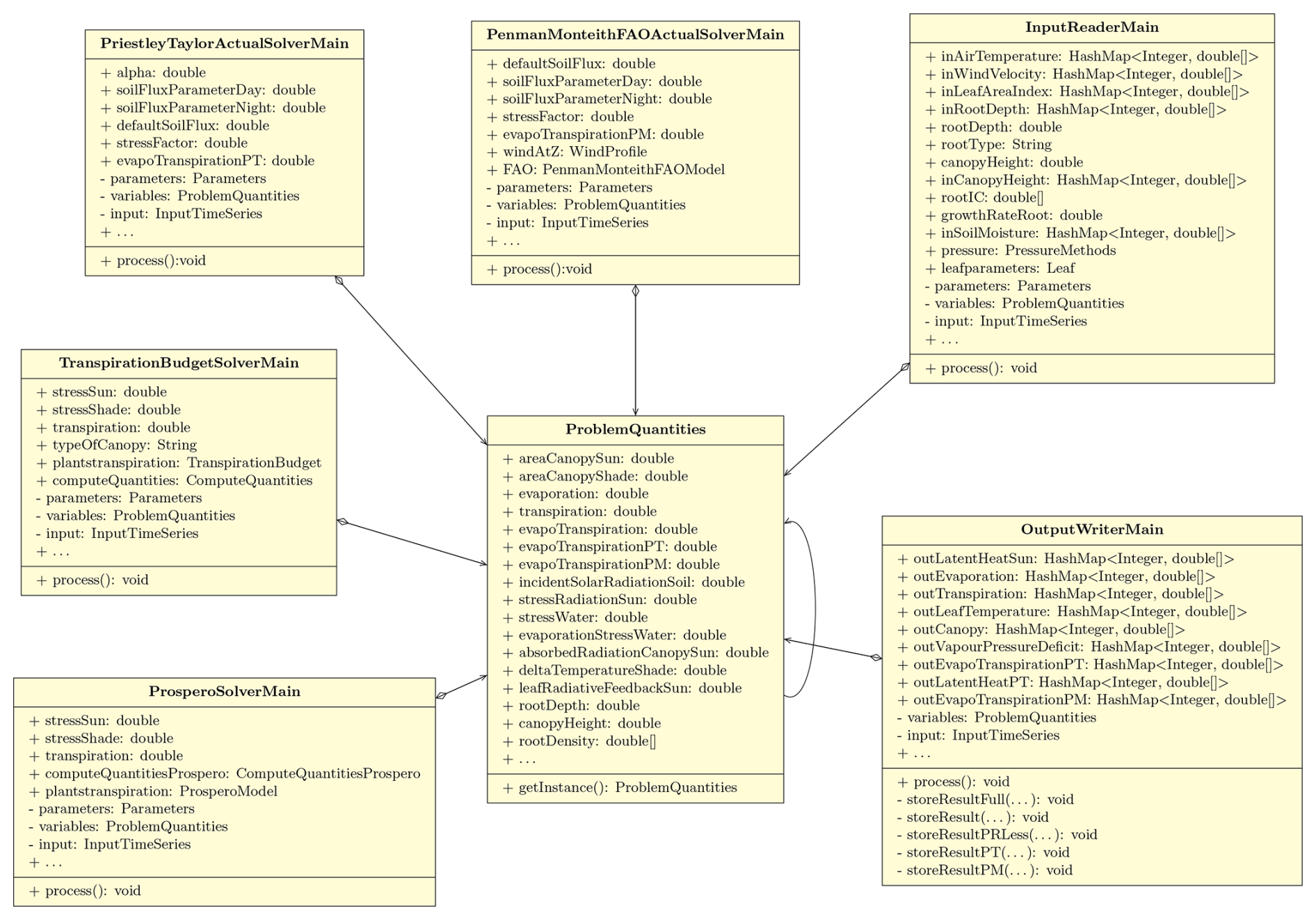
Figure A1 UML class diagram for the ProblemQuantities class, illustrating the aggregation and association relations with the ET model solver classes and mainly with the input and output classes. In this way we ensure that all model variables are shared among all classes regardless of the type of ET model used.

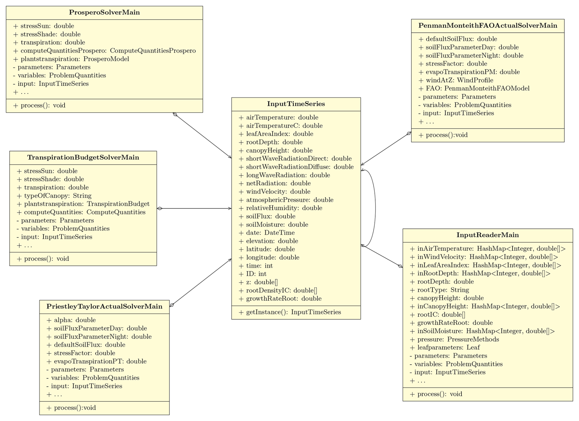
Figure A2 UML class diagram for the InputTimeSeries class, revealing the aggregation and association relations with some of the classes involved.