PyESPERv1.0.0: a Python implementation of empirical seawater property estimation routines (ESPERs)

This project produced a Python language implementation of locally interpolated regression (LIR) and neural network (NN) algorithms from empirical seawater property estimation routines (PyESPERv1.0.0). These routines estimate total alkalinity, dissolved inorganic carbon, total pH, nitrate, phosphate, silicate, and oxygen from geographic coordinates, depth, salinity, and 16 combinations of zero to four additional predictors (temperature and biogeochemical information) and were previously available only in the MATLAB programming language. Here, we document modifications to reduce discrepancies between the implementations, calculate the disagreements between the methods, and quantify Global Ocean Data Analysis Project (GLODAPv2.2022) reconstruction errors with PyESPER. While the PyESPER routine based on neural networks (PyESPER_NN) faithfully reproduces the corresponding MATLAB routine estimates of properties that do not require anthropogenic carbon change information, PyESPER_LIR and – to a lesser extent – PyESPER_NN estimates for total pH and dissolved inorganic carbon do not exactly reproduce the MATLAB routine estimates due to differences in interpolation and extrapolation methods between the programming languages. While the MATLAB and Python LIR-based estimates are not identical, we show that they are similarly skilled at reproducing the GLODAPv2.2022 data product and are thus comparable. This project increases the accessibility of ESPERv1.01.01 algorithms by providing users with code in the freely available Python language and enables future ESPER updates to be released in multiple coding languages.

1 Introduction

Ship-based biogeochemical data, as compiled within the Global Ocean Data Analysis Project (GLODAP; Lauvset et al., 2022), have high precision and accuracy but are seasonally biased and spatially sparse (Hauck et al., 2023). International efforts to deploy biogeochemical (BGC) profiling floats with broad spatial coverage and high temporal resolution (10 d) are ongoing (Bittig et al., 2019), with potential to greatly augment available ocean carbon cycle and biogeochemical data. These data can then support a wide variety of research topics and management applications (e.g., warming, acidification, eutrophication, deoxygenation, fisheries, and ecosystem studies). This strategy leverages the high precision and accuracy of ship-based measurements to calibrate and validate the BGC float sensors periodically throughout a float deployment. To do this, machine learning and regression algorithms – which take advantage of the strong regional correlations between seawater properties in the open ocean and, especially, the ocean interior (Bittig et al., 2018; Carter et al., 2018, 2021) – are used to map the ship-based information onto “reference depth” portions of the float profiles.

The empirical seawater property estimation routines (ESPERv1.01.01, henceforth referred to as ESPERs), originally written in the MATLAB programming language, aim to help realize the full potential of BGC float data by using machine learning techniques and regression strategies to predict total alkalinity (TA), dissolved inorganic carbon (DIC), pH on the total scale (pH_T), phosphate, nitrate, silicate, and oxygen from commonly measured physical and BGC parameters (Carter et al., 2021). The algorithms are used to calibrate float profiles (Maurer et al., 2021). In addition, because two carbonate system property measurements are necessary to fully quantify the carbonate system in seawater (Zeebe and Wolf-Gladrow, 2001) and BGC floats only have the capability to measure pH_T, these algorithms have the potential to provide (calculated) TA or DIC as a secondary constraint for the marine carbonate system. This method also offers an alternative to using models to estimate variables for carbonate chemistry calculations when nutrient information is unavailable, which potentially has high error values. ESPERs have also been used to map ship-based information across spatial and temporal scales for other applications, including estimation of TA for adjustments of the pH and fugacity of CO₂ (fCO₂) to in situ conditions for data products (Jiang et al., 2021) and estimation of the TA and seawater properties necessary for estimating ocean acidification indicators (Jiang et al., 2020; Sharp et al., 2024). Recent research has also shown that similar machine learning estimation algorithms have potential for the development of four-dimensional data products such as the Gridded Ocean Biogeochemistry from Artificial Intelligence–Oxygen (GOBAI-O₂; Sharp et al., 2023) and the Mapped Observation-Based Oceanic DIC (MOBO-DIC; Keppler et al., 2020).

1.1 Importance

Tanhua et al. (2021) and others have argued that researchers should utilize workflows that produce findable, accessible, interoperable, and reusable (FAIR) data products. ESPERs are publicly available (findable) on Zenodo, with updates published to GitHub, are free (accessible), and provide the option for users to cite a digital object identifier (DOI) for each version (reusable). However, until now, ESPERs were available only in the proprietary MATLAB programming language, which posed a barrier to accessibility and interoperability that we aim to address. Future updates may include even more accessible features such as a user interface.

1.2 Goals

This project aimed to create a freely available Python implementation of ESPERs (PyESPERv1.0.0, henceforth referred to as PyESPERs; Carter et al., 2021; Dias and Carter, 2025) that is equivalent to the MATLAB version within ±2 times the estimate uncertainties (σ) for all estimated biogeochemical properties (TA, DIC, pH_T, nitrate, phosphate, silicate, and oxygen). The PyESPER code is freely available at Zenodo, and updates will be made available at the GitHub repository (see the “Code availability” section).

2 Methods

ESPER algorithms were translated into Python coding language, while the associated files were either translated into Python or read by Python as MATLAB files. Some original methods were required to allow interpolations to be similar in Python to those of MATLAB ESPERs.

2.1 ESPERs

ESPERs allow estimation of biogeochemical seawater properties using coordinates, depth, salinity, and other optional inputs from a single function call. While sharing a similar set of equations and required input data, ESPERs have two variants that use either locally interpolated regressions (ESPER_LIR) or neural networks (ESPER_NN), along with a mixed estimate (ESPER_Mixed) that is the mean of estimates from the two functions (Carter et al., 2021). There are a couple of reasons to maintain the separate ESPER LIR, NN, or Mixed options, from an end-user perspective, and these reasons are also true for PyESPERs.

1. ESPER_LIRs predate the ESPER_NNs and have been used as a standalone data product for various research purposes (see Carter et al., 2016, 2018). Long-term users of these LIRs have previously expressed a desire for consistency between versions (e.g., when depth was taken out as a predictor for pH_T), and some of them already use CANYON-B (Bittig et al., 2019) as a neural network option for comparison. Therefore, these users who desire consistency would most likely prefer to use ESPER_LIR.

2. ESPER_LIRs are more transparent than ESPER_NNs, as it is simple to parse apart coefficients at the gridded locations and to see how the equations are a result of these. ESPER_LIRs also rely on a grid, which may appeal to some users.

3. ESPER_NNs provide improved estimates on average compared with ESPER_LIRs and behave more like a mapping product in that 3D coordinates are predictors, which may alternately appeal to some users.

4. Although the ESPER_Mixed estimates perform better on average than LIRs or NNs do independently, there are cases where they have greater bias and root mean square error (RMSE) values than LIRs or NNs (e.g., when using Eqs. 1–3 for phosphate or nitrate at all depths; Carter et al., 2021). Users may want to assess each scenario independently and choose which method is most appropriate according to their needs.

5. The NNs are more closely reproduced between the MATLAB and Python ESPER implementations.

2.1.1 Locally interpolated regressions

The most recent versions of ESPER_LIRs (version 1.01.01; version 3 of LIRs) use a standard set of equations of the format shown in Eq. (1) to estimate up to seven different biogeochemical water properties using up to 16 equations with different combinations of input parameters (see Appendix A, Tables A1 and A2; Carter et al., 2021):

$$\begin{array}{}\text{(1)}& X=C_{\mathrm{0}}+\sum _{i=\mathrm{1}}^n{C}_i{P}_i,\end{array}$$

where X is the estimated property (TA, DIC, pH_T, nitrate, phosphate, silicate, or oxygen), C₀ is the intercept, and C_i is the coefficient for each of the n predictors P_i. The intercepts (C₀) and coefficients (C_i) vary with location (latitude, longitude, and depth) and are different for each of the predictor variables (P_i; Tables A1 and A2; Carter et al., 2021). The most recent ESPERs were trained and assessed on the GLODAPv2.2020 (Olsen et al., 2020) data product, which includes data from 946 cruises and spans 1972–2019, and additional datasets from the Mediterranean Sea and Gulf of Mexico (Carter et al., 2021, Supplementary Information) taken from the Coastal Ocean Data Analysis Project (CODAP, Jiang et al., 2021) and the CARIMED data product (Álvarez et al., 2019).

When the ESPER_LIR function is called, the routines interpolate a pre-determined grid of C's (intercepts and coefficients) to user-defined locations. Linear interpolation is used within the grid and for extrapolation, and this method utilizes an underlying Delaunay triangulation with MATLAB's scatteredInterpolant function (Carter et al., 2021). The three-dimensional interpolation and extrapolation algorithm is implemented differently in MATLAB and Python, and although both calculations are valid, this difference in implementation is the source of disagreements we find and later quantify between ESPER and PyESPER.

ESPER_LIR coefficients have been determined on a grid using a moving window regression strategy similar to the approach first outlined by Velo et al. (2013), resulting in a set of intercept and coefficient estimates for each of 16 equations for seven possible properties at 44 957 total locations on a 5° latitude (−84.5–85.5° N) × 5° longitude (−19.5–375.5° E) × 33 depth (0–5500 m) ocean interior grid subsampled from the World Ocean Atlas gridded product (Carter et al., 2016, 2018, 2021). These coefficients were fit using regressions relating the property of interest (X) to different combinations of up to five predictor properties (P, Tables A1 and A2), relating to each possible equation as in Eq. (1). Depth (scaled to $\mathrm{1}/\mathrm{25}$) is included as a coordinate for coefficient interpolation, but depth is not used as a predictor for the current ESPER version (it was included in an earlier version, but only when predicting pH_T; Carter et al., 2018). Data for each regression fit are selected from “windows” of data that are within 15° latitude, within 30°$/$cosine(latitude) in longitude, and within either ($\mathrm{100}+z/\mathrm{10}$) m depth or 0.1 kg m⁻³ of the estimated density of seawater at that coordinate location, where z is depth in meters (Carter et al., 2021). If either the depth-based or the density-based criterion applies, data are selected for that location, which allows water masses to impact window selection along with depth. If fewer than 100 measurements fall within a window, the dimensions are doubled. In LIRv2, windows are iteratively scaled by a factor of the iteration number until at least 100 measurements are selected to train each regression (Carter et al., 2018). For ESPER_LIRs (LIRv3), it is argued that increasing window size has the following benefits: (1) includes more data for regression fits, (2) introduces more modes of oceanographic variability into fitting data, and (3) reduces multicollinearity (Carter et al., 2021). However, the risk of increasing the window size is that the ESPER_LIRs will be less appropriate locally. A weighting term is applied to help account for this by reducing the cost of regression misfits to data that are distant or at significantly different depths relative to the location, with a cap to prevent overfitting to nearby coordinates (see Carter et al., 2021). Regression coefficients (C₀ and C_i) are then fit using Eq. (2), with separate regressions for the Northern Hemisphere Atlantic, Mediterranean, and Arctic, as well as other global locations, to prevent interpolation across Central America or the Bering Strait.

$$\begin{array}{}\text{(2)}& \text{XW}=\left(C_{\mathrm{0}}+\sum _{i=\mathrm{1}}^n{C}_i{P}_i\right)W\end{array}$$

PyESPER_LIR does not duplicate this portion of the effort but instead builds directly upon the grid of coefficients obtained for and utilized by the MATLAB implementation of ESPER_LIR.

When the function is called, ESPER_LIR uses MATLAB's scatteredInterpolant (linear interpolation and extrapolations) function to interpolate this previously created grid of regression coefficients to the user-provided set of coordinates, resulting in coefficient estimates at the desired locations (Carter et al., 2021). This method uses a Delaunay triangulation of the scattered sample points to perform interpolations and extrapolations. Different valid mathematics can be used to obtain these Delaunay triangulations and to extrapolate and interpolate, but efforts to identify a Python method for these tasks that exactly replicates the MATLAB results have been unsuccessful. The most similar and least computationally intensive results relative to those of MATLAB's scatteredInterpolant were produced by combining Python's SciPy package functions LinearNDInterpolator (interpolate subpackage) and Delaunay (spatial subpackage; Virtanen et al., 2020). However, because LinearNDInterpolator does not extrapolate and other Python functions do not produce similar results to those of MATLAB when using similar methods, the gridded set of three-dimensional coordinates (44 957 locations based on the World Ocean Atlas) and corresponding coefficient estimates provided by ESPER_LIRs were expanded in MATLAB to 106 400 locations on a grid with estimates every 5° latitude (−94.5–90.5° N) and longitude (−19.5–375.5° E) and up to 9000 m in depth and applied to scatteredInterpolant within ESPER_LIR to provide coefficient estimates for the external locations through extrapolation. This grid, with equivalent coefficients within the original parts of the grid and extrapolations outside of the grid, was read in Python when the LIRs were called. The expanded grid allowed Python functions to avoid extrapolations and rely solely on interpolation and triangulation methods when estimating coefficients at user-defined locations. While some of these locations are unphysical (e.g., $\pm >\mathrm{90}\mathit{°}$ N or on land), the coefficients nevertheless provide valid extrapolations from MATLAB for the full possible domain that can then be interpolated in PyESPER_LIR. PyESPER_LIR otherwise replicated ESPER_LIR's separation of data from the Atlantic Ocean, Mediterranean Sea, and Arctic Ocean and data from the Indo-Pacific and Southern Ocean regions.

During the creation of this expanded grid, a grouping error was observed in current versions of MATLAB ESPER_LIRs. Specifically, the mirrored portion of the grid found at <0 and >360° E and north of 40° S was not correctly flagged as belonging to the Atlantic grid. The practical effect of this bug was that estimates near the Prime Meridian and near the cutoff between the Southern Ocean and the Atlantic Ocean had extrapolated coefficients instead of interpolated coefficients. This bug was fixed for both MATLAB ESPER_LIR and PyESPER_LIR comparisons for this paper, and a fixed grouping routine is now provided at the original MATLAB ESPER repository with corresponding documentation and will be included in future updates to ESPER_LIRs.

2.1.2 Neural networks

ESPER_NNs use feed-forward neural networks with latitude, depth, cosine(longitude − 20° E), cosine(longitude − 110° E), and the parameters from Table A2 as predictors. Four neural networks are used in each of the two ocean regions, which are the same as those used for LIRs (Atlantic–Mediterranean–Arctic and Indo–Pacific–Southern), resulting in 896 total neural networks (eight for each of 16 combinations of predictors for seven property estimates; Carter et al., 2021). An ensemble of four previously created neural networks with different combinations of neurons and hidden layers, including a single one-hidden-layer network with 40 neurons and three two-hidden-layer networks with $\mathrm{30}/\mathrm{10}$, $\mathrm{25}/\mathrm{15}$, and $\mathrm{20}/\mathrm{20}$ neurons in the first/second hidden layers, is used to minimize the impact of errors from any one neural network (Carter et al., 2021).

In ESPER_NN, the neural networks are encoded as functions to avoid requiring access to the machine learning toolbox within MATLAB. Here, we further translate these functions to Python. The resultant Python functions replicate the functions in ESPER_NN to within machine precision. ESPER_NNs linearly interpolate between the two regions of neural networks by latitude across the Southern Atlantic Ocean and Bering Sea and between the North Pacific and Arctic oceans. Zonal transitions in the Southern Atlantic and Indo–Pacific–Southern Ocean network are also implemented. This interpolation uses custom-written 1D or 2D interpolations that are handled identically in both programming environments.

2.1.3 Mixed estimates

The mixed estimate for each input location is the mean of the LIR and NN estimates and therefore is trivially reproduced by a simple single function call and module within Python.

2.1.4 Anthropogenic carbon

The impacts of anthropogenic carbon (C_ant) are approximated in ESPER and PyESPER using a 1°×1° gridded transit time distribution (Waugh et al., 2006) C_ant product referenced to the year 2002 (Lauvset et al., 2016). ESPERs assume that oceanic C_ant increases proportionally to atmospheric anthropogenic CO₂ (transient steady-state assumptions; Gammon et al., 1982; Gruber et al., 2019; Tanhua et al., 2007). This implies that the “shape” of the C_ant vertical profile (gradient) remains constant with continuous exponential increases in atmospheric CO₂ and ocean C_ant according to Eq. (3) (Carter et al., 2021).

$$\begin{array}{}\text{(3)}& C_{\text{ant\_year\_location}}=C_{\text{ant\_year\_location}}{\mathrm{e}}^{\mathrm{0.018989}(\text{year}-\mathrm{2002})}\end{array}$$

The coefficient in Eq. (3) is derived from Gruber et al.'s (2019) assumption of a 28 % increase in C_ant from 1994 to 2007 and enables estimating C_ant for a location in a desired year when C_ant is known for that same location in a reference year (2002; Carter et al., 2021). This approach does not allow for non-steady-state variations, which is accounted for in overall uncertainty estimates, and is noted as a significant source of uncertainty for projections beyond ∼2030.

ESPERs were trained on data for pH_T and DIC, which were converted to the equivalents for the year 2002, and then modified back to the original measurement dates using Eq. (3). ESPERs and PyESPERs estimate the C_ant component of DIC and pH_T in output variables for 2002 by interpolating the 2002 C_ant grid to user-provided coordinates and then applying Eq. (3) to estimate C_ant for the user-requested estimate year. As with the original ESPERs, this method is not meant to be used when C_ant is of primary interest but rather provides a means of quickly adjusting DIC or pH_T to a reference year (Carter et al., 2021). Likewise, these methods are not adequate for making reliable projections beyond the year 2030, or perhaps sooner in coastal or other areas where the underlying global open ocean anthropogenic carbon estimations have greater uncertainties (Carter et al., 2021).

2.2 Uncertainty estimation

ESPERs and PyESPERs return depth- and salinity-dependent uncertainties for each property at the 1σ (one standard uncertainty) level, meaning approximately 95 % of new open ocean measurements from GLODAPv2.2022 should fall within ± twice the ESPER uncertainties (Carter et al., 2021). As in Carter et al. (2021), baseline error estimates in the depth and salinity space (E_{X_Est}) are interpolated based on RMSEs of all predictions from validation versions of the routines within bins of salinity and depth. ESPER_LIRs and PyESPER_LIRs scale these uncertainties using user-provided predictor uncertainty estimates (E_{Pi_Provided}). Equation (4) is used when user-provided uncertainties exceed the default assumed input uncertainties (E_{Pi_Default}; Table A3):

$$\begin{array}{}\text{(4)}& E_{X\mathit{\_}\text{Output}}=\sqrt{\begin{array}{l}{E}_{X\mathit{\_}\text{Est}}^{\mathrm{2}}-\sum _{i=\mathrm{1}}^n{\left(\frac{\partial X}{\partial P_i}{E}_{\text{Pi\_Default}}\right)}^{\mathrm{2}}\\ +\sum _{i=\mathrm{1}}^n{\left(\frac{\partial X}{\partial P_i}{E}_{\text{Pi\_Provided}}\right)}^{\mathrm{2}}\end{array},}\end{array}$$

where $\frac{\partial X}{\partial P_i}$ is the sensitivity of the property estimate X to the ith predictor P_i. ESPER_NNs and PyESPER_NNs estimate sensitivities by iteratively perturbing the input predictors if the user specifies uncertainties that are larger than the default. Mixed uncertainties are the minimum uncertainties assessed for LIR and NN estimates.

2.3 Assessment

For many applications, the most critical validation is a test of the reconstruction of withheld data. However, such an exercise requires training alternative versions of the method after withholding data, and, as of now, PyESPER is not separately trained but is instead reliant on the ESPER training that was performed and validated previously with MATLAB (Carter et al., 2021). For this publication, we aim to instead show that PyESPER and ESPER provide quantitatively similar results and assert that the validation presented earlier for ESPER in MATLAB can be considered to also be appropriate for PyESPER in all but a limited number of specific exceptional cases. To support this claim, PyESPER and ESPER were used to estimate values for the GLODAPv2.2022 data product (1 381 248 sets of measurements; Fig. 1) with each equation and output variable combination. This dataset included a wide range of input data, and comparison of PyESPER and ESPER was primarily considered based on application to the high-quality “open ocean” (_o) portion of the GLODAP dataset as in Carter et al. (2021), defined as GLODAP data with only World Ocean Circulation Experiment (WOCE) data quality control flag categories of 2 (Acceptable) and secondary quality control flag categories of 1 (subjected to full secondary quality control) for all possible input and measurement data and for salinities between 30 and 37 (n=306 227 for TA, 343 580 for DIC, 199 304 for pH_T, and 764 301 for phosphate, nitrate, silicate, and oxygen). Additional comparison with the entire GLODAPv2.2022 dataset (“whole ocean” or _w), including NaNs and anomalous data with salinities <30 and temperatures<0 °C, which are not recommended for use with ESPERs, is presented in Appendix B. These comparisons are used as a rigorous test of the fidelity of the PyESPER estimates to the ESPER estimates. Resulting estimates were compared graphically and with the normalized root mean square error (RMSE_n; equivalent to RMSE divided by the mean of the MATLAB estimate for each variable) for each equation case globally and regionally and across depths. RMSE_n was used because it allows for comparison between variables of different scales. Additionally, where measured values were present in the dataset, both ESPER and PyESPER were validated against the measured data, though, again, this is not a validation of the method as much as a check that both variants provide similar values.

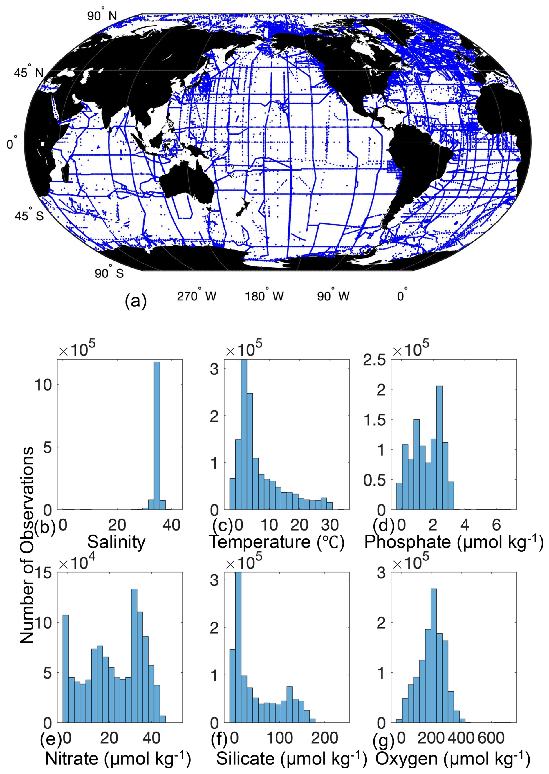
Figure 1 Location of GLODAPv2.2022 data used to compare PyESPER to MATLAB ESPER estimates (a), and histograms of the distributions of measured GLODAPv2.2022 variables used as inputs for the PyESPERv1.0.0 and ESPER algorithms (b–g).

2.3.1 DIC application

As an additional comparison of the LIR method differences, DIC estimates from both PyESPER_LIR and ESPER_LIR were applied to the Roemmich–Gilson Argo climatology (Roemmich and Gilson, 2009) to create mapped annual surface estimates of DIC.

3 Results and discussion

PyESPER and ESPER produced open ocean estimates with mean differences (Python estimate–MATLAB estimate) of $<\pm \mathrm{0.04}$ for all parameters, and NNs had smaller mean differences of $<\pm \mathrm{0.004}$ for all parameters (units are µmol kg⁻¹ except for pH_T) estimated from the open ocean GLODAPv2.2022 data, although the standard deviations of these differences and uncertainties associated with the estimates were at times larger than the mean differences (Tables 1 and 2). The greatest RMSE_n was $\mathrm{2.08}\times {\mathrm{10}}^{-\mathrm{2}}$ for silicate estimates using LIRs. PyESPER_NN functioned as an equivalent data product to ESPER_NN for all data. For open ocean data, PyESPER_LIRs functioned similarly to ESPER_LIRs, with a large majority of identical estimates produced between the two data products.

3.1 Data product validation

The results of comparisons between MATLAB ESPERs and PyESPERs are described below.

3.1.1 Locally interpolated regressions

When compared to the ESPER_LIR results for the open ocean (_o) GLODAPv2.2022 dataset, all equation–case and desired outcome variable combinations from PyESPER (PyESPER_LIR–ESPER_LIR estimates) resulted in mean differences of $<\pm \mathrm{0.04}$ (Table 1). Mean (± standard deviation; RMSE_n) PyESPER–ESPER_LIR differences for each property are shown in Table 1. The very wide range of input data resulted in a wide range of estimates from both ESPER_LIRs and PyESPER_LIRs for all variables (Table 1; Fig. 2; for _w, see Appendix B, Fig. B1), representing the large range of biogeochemical property values that can be found in the oceans. The PyESPER_LIR and ESPER_LIR results worked similarly well in predicting measured values at locations, even with the outlier and unusual input data used (see Table B1), suggesting that the Python estimates, although not identical to the MATLAB estimates for these interpolations, were equivalently valid reconstructions.

Table 1 Mean (standard deviation), maximum, minimum, and normalized RMSE (RMSE_n) for differences between MATLAB and Python LIRs, ESPER_LIR and measured values, and PyESPER_LIR and measured values for TA, DIC, pH_T, phosphate, nitrate, silicate, and oxygen estimates (all units, except for pH_T, are µmol kg⁻¹) for open ocean (_o) data and all equations combined (n=13 384 096 for TA, 13 384 096 for DIC, 13 384 096 for pH_T, 13 384 096 for phosphate, 12 718 592 for nitrate, 12 640 896 for silicate, and 12 757 792 for oxygen).

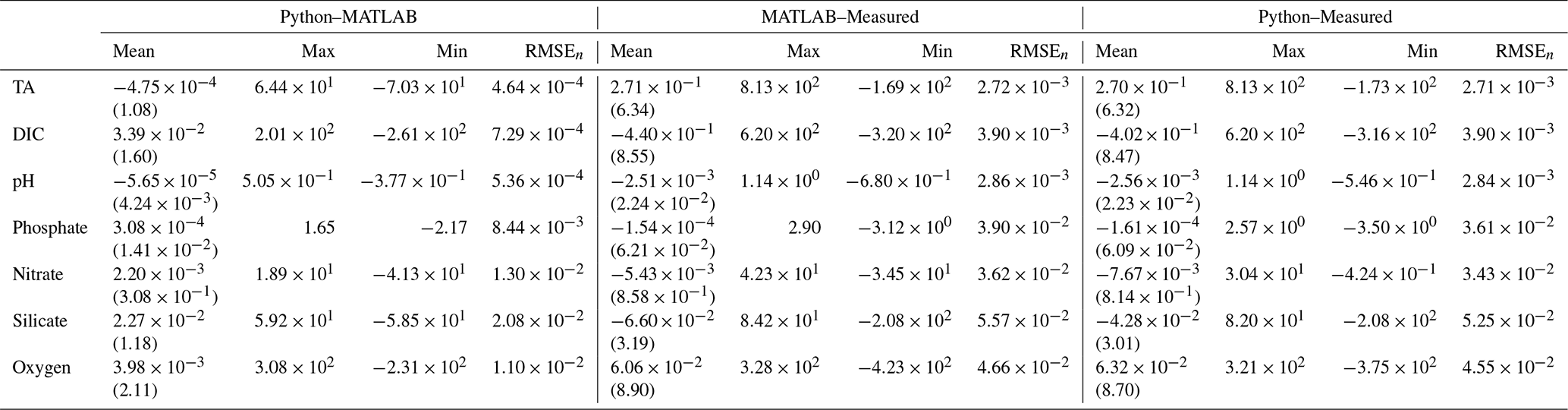
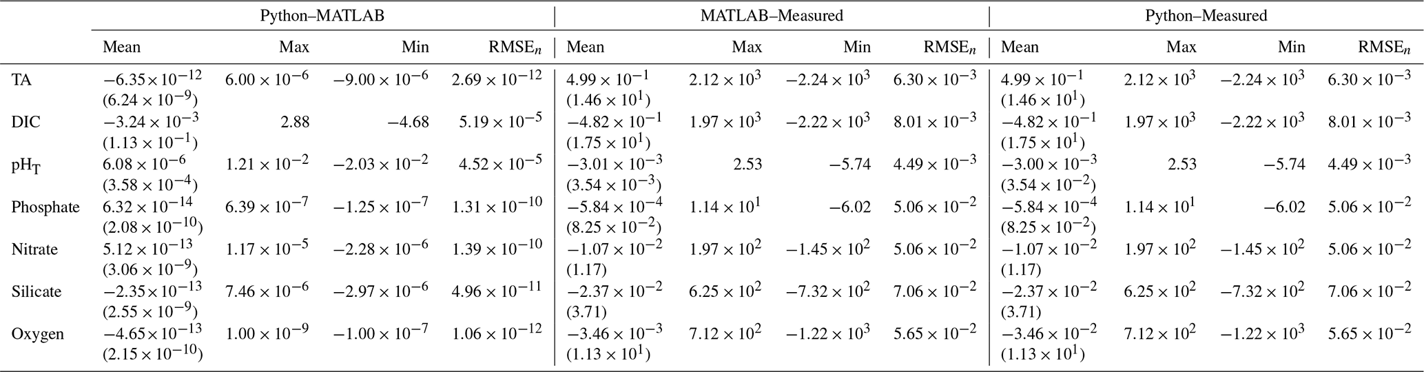
Table 2 Mean (standard deviation), maximum, minimum, and normalized RMSE (RMSE_n) are shown for three scenarios: (1) between Python and MATLAB NNs, (2) between MATLAB ESPER_NN and measured values, and (3) between PyESPER_NN and measured values. Separate rows exist for TA, DIC, pH_T, phosphate, nitrate, silicate, and oxygen estimates. All units, except for pH_T, are µmol kg⁻¹, and data are for open oceans (_o) and all equations combined.

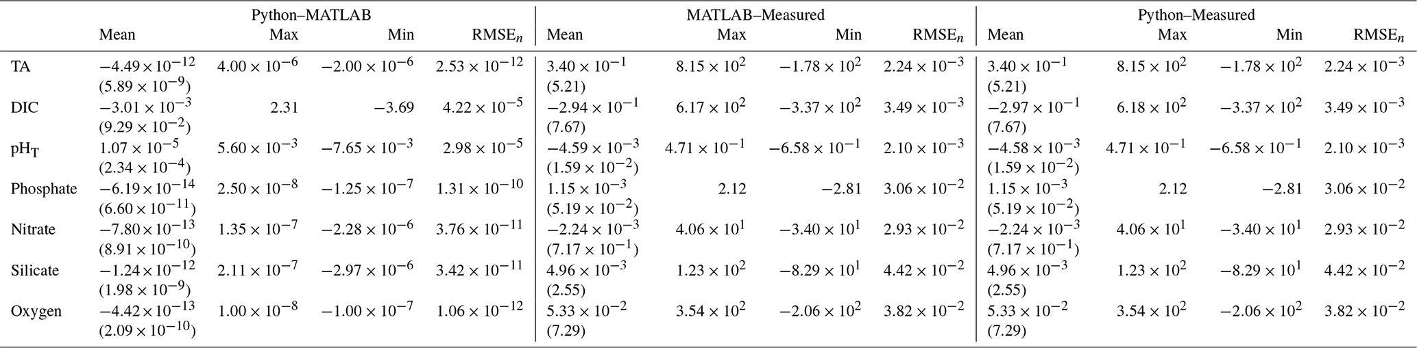
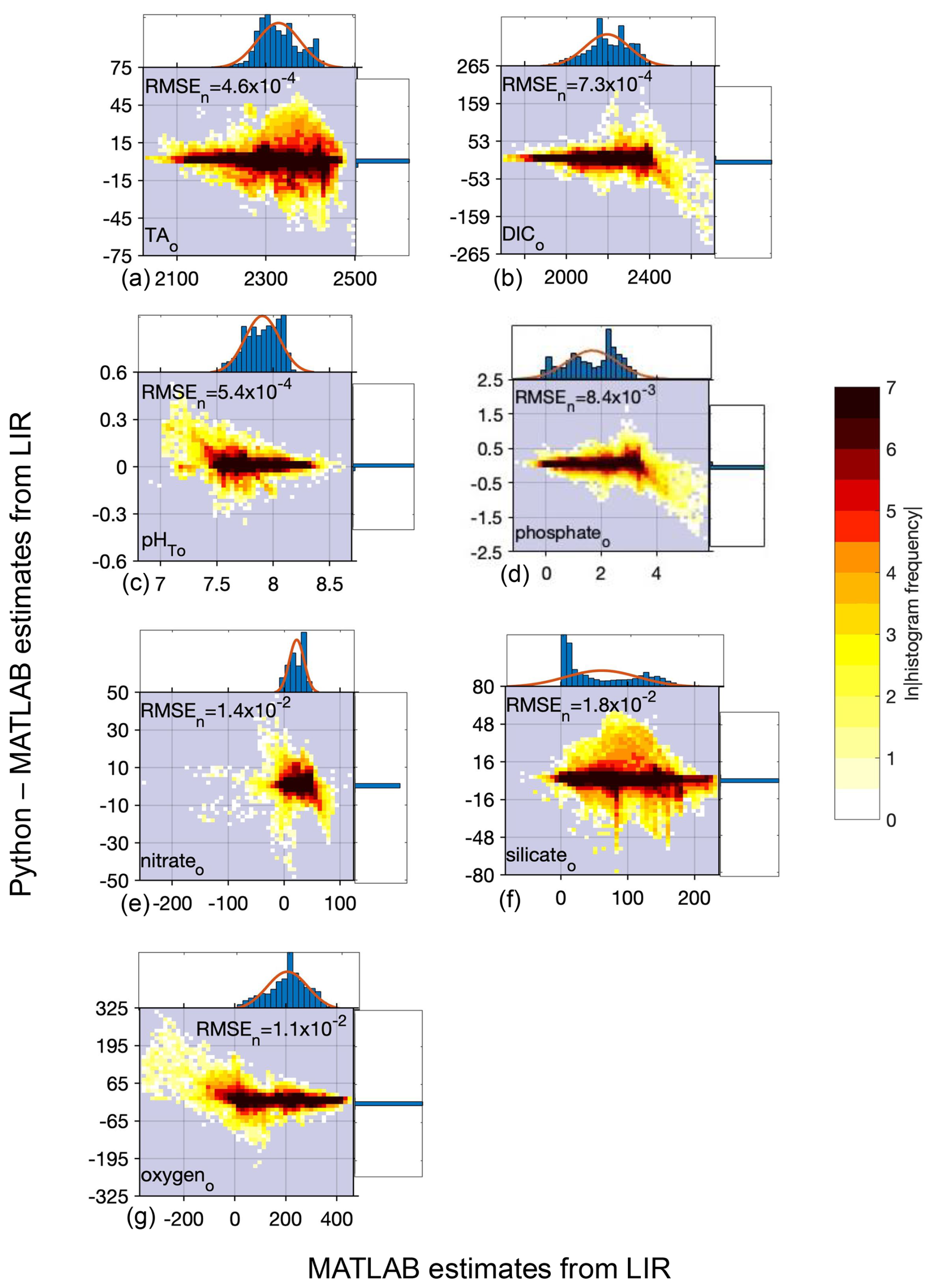
Figure 2 Difference between Python and MATLAB locally interpolated regression estimates (y axis) compared to MATLAB estimates (x axis) for open ocean (_o) data and all equations combined for TA (a, 13 384 096 total estimates from all equations), DIC (b, 13 384 096 estimates), pH_T (c, 13 384 096 estimates), phosphate (d, 13 384 096 estimates), nitrate (e, 12 718 592 estimates), silicate (f, 12 640 896), and oxygen (g, 12 757 792 estimates); n= 306 227 for TA, 343 580 for DIC, 199 304 for pH_T, and 764 301 for phosphate, nitrate, silicate, and oxygen. All units, except for pH_T, are µmol kg⁻¹. Top and side histograms represent the distribution of the x and y axes, respectively. Note the differences in the x- and y-axis scales. RMSE_n is the normalized root mean square error, or the RMSE of all estimates divided by the mean of all estimates.

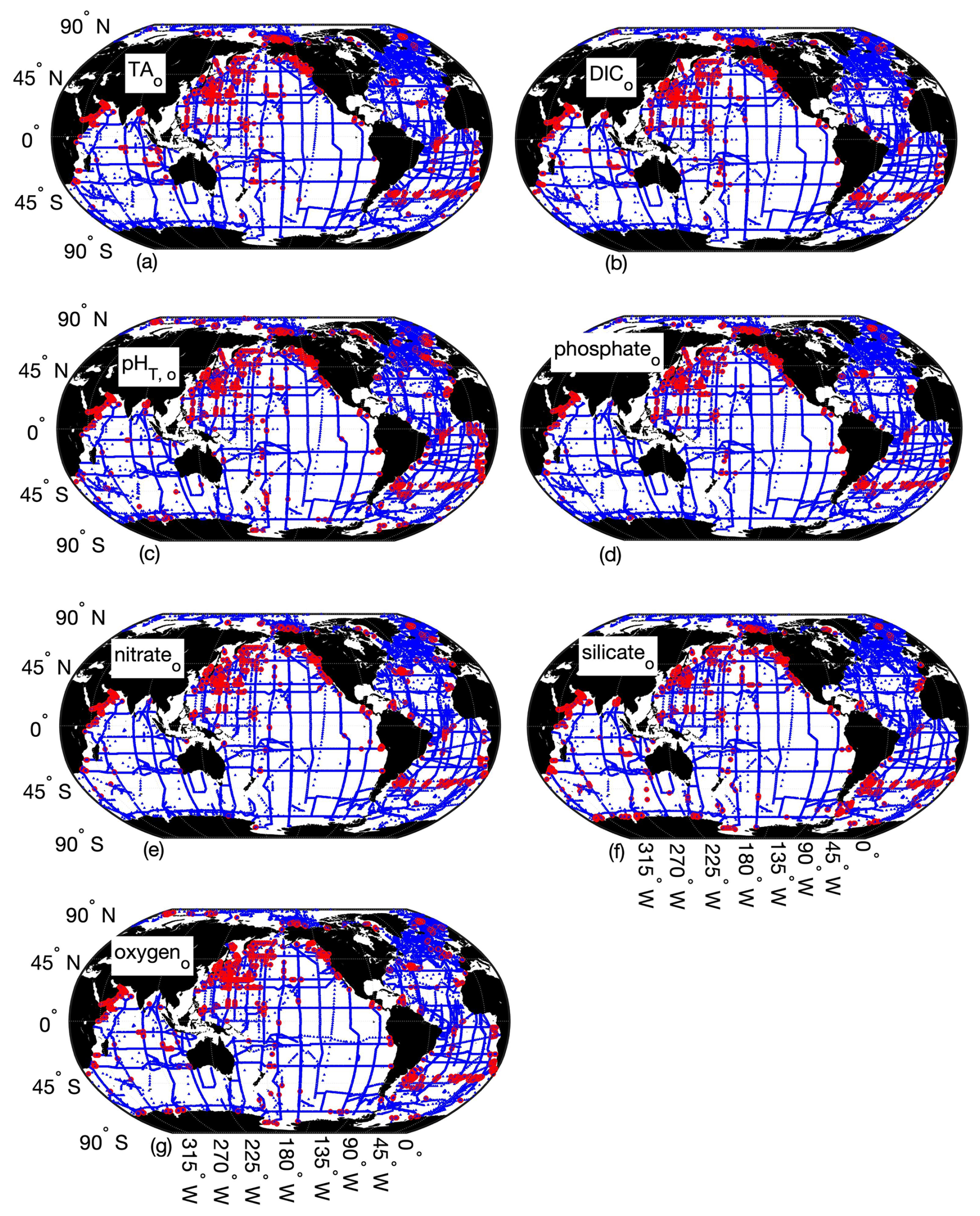
Figure 3 Map of differences between Python and MATLAB ESPER locally interpolated regression estimates (total estimates n=13 384 096 for TA (a), DIC (b), pH_T (c), and phosphate, 12 718 592 for nitrate (d), 12 640 896 for silicate (e), and 12 757 792 for oxygen (f)) for the open ocean (_o), where the small blue circles represent differences<2 times the uncertainties of the MATLAB estimates (n=13 344 924 for TA, 13 354 980 for DIC, 13 349 438 for pH_T, 13 357 843 for phosphate, 12 688 861 for nitrate, 12 597 608 for silicate, and 12 721 483 for oxygen) and red circles represent differences>2 times the uncertainties of the MATLAB estimates (n=39 172 for TA, 29 116 for DIC, 34 658 for pH_T, 26 253 for phosphate, 29 731 for nitrate, 43 288 for silicate, and 36 309 for oxygen).

PyESPER_LIRs were within 2σ (∼95 % of measurements should fall within this uncertainty level) for most ocean regions, with a few exceptions that occurred predominantly in coastal areas or deep waters near the edges of the original MATLAB grid (Figs. 3 and 4). Spatial patterns in the distribution of outliers shown in Fig. 4 appear to reflect locations where more edge-of-grid biogeochemical measurements were collected (e.g., near coasts and in deep waters). Hence, these exceptionally different locations aligned well with places where coefficients were extrapolated in MATLAB for use in PyESPER_LIRs, compared to interpolations with distant “dummy points” within MATLAB ESPER_LIRs (see Sect. 2.1.1, Locally interpolated regressions, Figs. 3–5; for _w, Figs. B2 and B3). Within regions where MATLAB and Python were interpolating similarly, far outliers were uncommon (Figs. 3–5, B2, and B3). When ESPER_LIR and PyESPER_LIR were applied to temperature and salinity from the Roemmich and Gilson climatology for the year 2023 (Roemmich and Gilson, 2009), the patterns of the surface DIC distribution were similar, with a few minor nuances (Fig. C1). Notably, low DIC estimates covered a broader spatial extent in the western equatorial Pacific and Indian oceans for the PyESPER_LIR estimates, and PyESPER_LIR appeared to have a slightly low bias in some places relative to ESPER_LIR. Beyond these minor differences, the mapped DIC demonstrates the similarity of the data products' functionality in an applied setting. While ESPER_LIR and PyESPER_LIR do not produce quantitatively identical estimates, it should be noted that both routines perform similarly well at reconstructing the GLODAPv2.2022 data product (Table 1; for _w, Table B1). These routines should not be considered identical but are comparable.

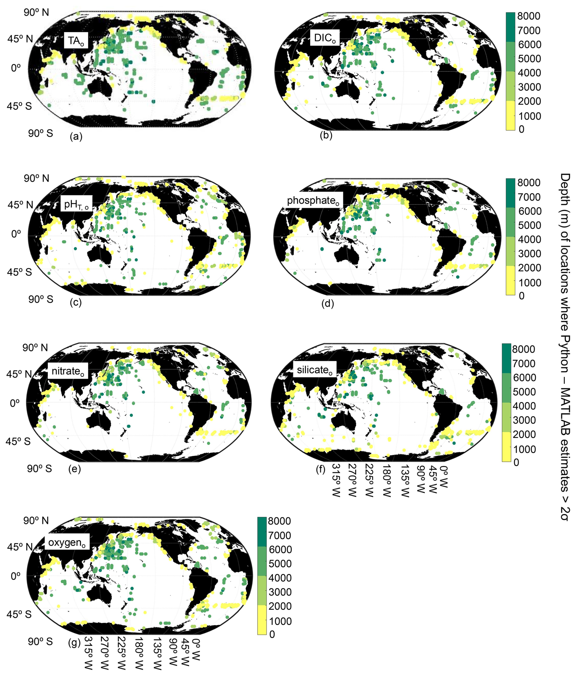
Figure 4 Map of locations and depths (color bar) where differences between Python and MATLAB ESPER locally interpolated regression estimates are greater than 2 times the estimate uncertainties for the open ocean (_o; n=13 344 924 for TA (a), 13 354 980 for DIC (b), 13 349 438 for pH_T (c), 13 357 843 for phosphate (d), 12 688 861 for nitrate (e), 12 597 608 for silicate (f), and 12 721 483 for oxygen (g)).

3.1.2 Neural networks

When compared to the ESPER_NN results for the open ocean (_o) GLODAPv2.2022 dataset, all equation–case and desired outcome variable combinations from PyESPER_NN (PyESPER–ESPER_NN estimates) resulted in mean differences of $<\pm \mathrm{0.004}$ (Table 2), a much smaller difference than for the LIR comparisons. The mean (± standard deviation; RMSE_n) offset for each property is shown in Table 2. Because a very wide range of input data were used, a wide range of estimates were produced from both ESPER_NNs and PyESPER_NNs for all variables (Fig. 6), representing the high variability that can be found in the oceans (especially coastal regions, some of which were included in the “open ocean” dataset due to having salinities between 30 and 37 and quality-controlled data). Both the PyESPER_NN and ESPER_NN results were nearly identical, even when outlier results were obtained from unusual input data from environments where ESPERs are not recommended for use (for example, resulting in negative DIC estimates in Fig. B4; see also Table B2). The largest relative disagreements were found for DIC and pH_T, though these disagreements remained small relative to the measurement uncertainties. These minor offsets are attributed to the programming language differences in the interpolation of the C_ant adjustment, which is applied only to these two properties.

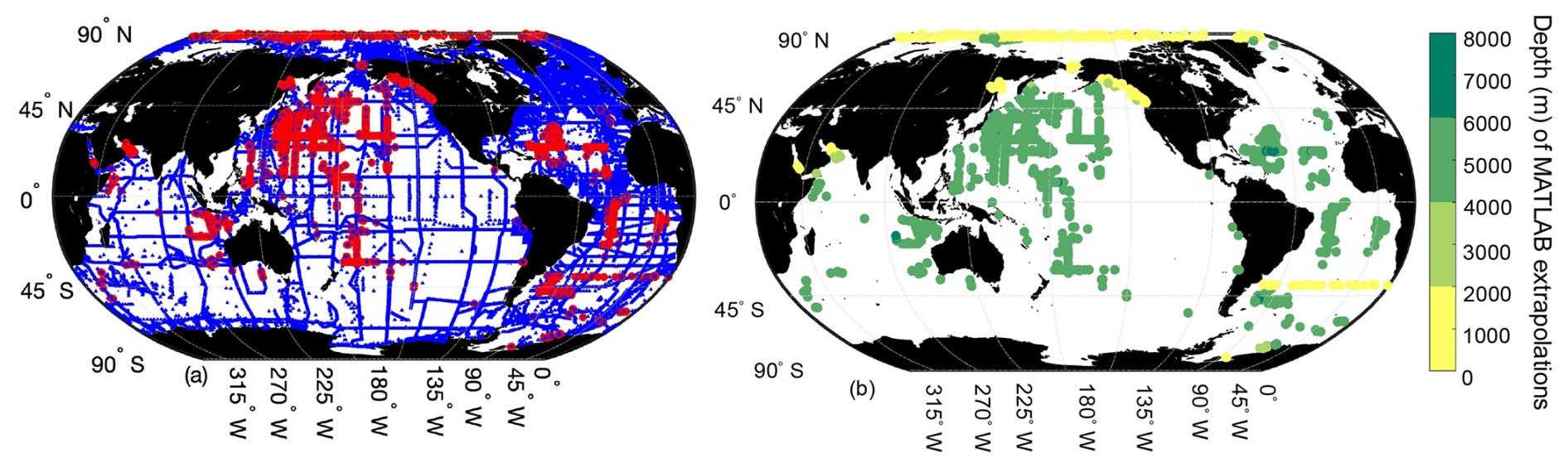
Figure 5 Map of locations where MATLAB was interpolating (n=1 365 170, blue) and extrapolating (n=16 078, red) from the grid to the GLODAPv2.2022 data (a), and the depth of the extrapolations (b).

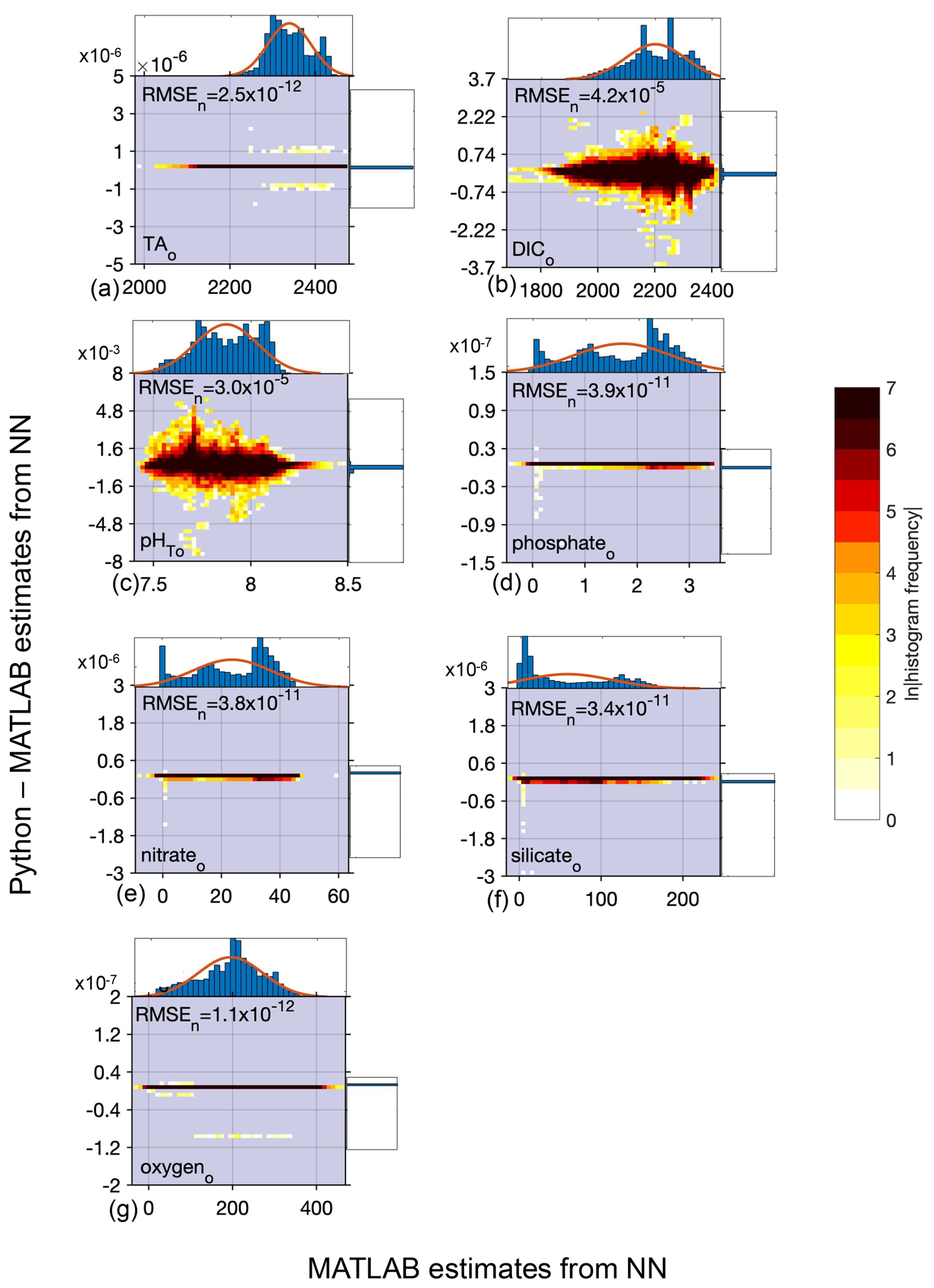
Figure 6 Difference between Python and MATLAB neural network estimates (y axis) compared to MATLAB estimates (x axis) for open ocean (_o) data and all equations combined for TA (a, 4 899 512 total estimates from all equations), DIC (b, 5 497 004 estimates), pH_T (c, 3 188 864 estimates), phosphate (d, 12 228 432 estimates), nitrate (e, 12 228 432 estimates), silicate (f, 12 228 432 estimates), and oxygen (g, 12 228 560 estimates); n=306 227 for TA, 343 580 for DIC, 199 304 for pH_T, and 764 301 for phosphate, nitrate, silicate, and oxygen. All units, except for pH_T, are µmol kg⁻¹. Top and side histograms represent the distribution of the x and y axes, respectively. Note the differences in the x- and y-axis scales. RMSE_n is the normalized root mean square error, or the RMSE divided by the mean of all estimates from MATLAB_NN.

3.1.3 Anthropogenic carbon estimates

Although inconsistencies in the results occur between Python and MATLAB when interpolating (same issue noted in Sect. 2.1.4, Anthropogenic carbon), the anthropogenic carbon (C_ant) estimates were similar between the two versions of ESPER. This was demonstrated by differences in the DIC and pH_T estimates for NNs, which interpolate only when estimating the contribution of C_ant to the estimates (Fig. 6). The next generation of ESPER updates will include a new method for estimating C_ant (Tracer-Based Rapid Anthropogenic Carbon Estimation, or TRACEv1; Carter et al., 2025), which uses neural networks and should eliminate the need for interpolation. Currently, when C_ant estimates are required, the results from PyESPER_NNs remain functionally identical to those from ESPER_NNs, despite minor offsets from the interpolation methods.

Table 3 Time required to produce estimates for PyESPERv1.0.0 and ESPERs (LIRs and NNs) for different desired variables, equation–case combinations, and numbers of estimates.

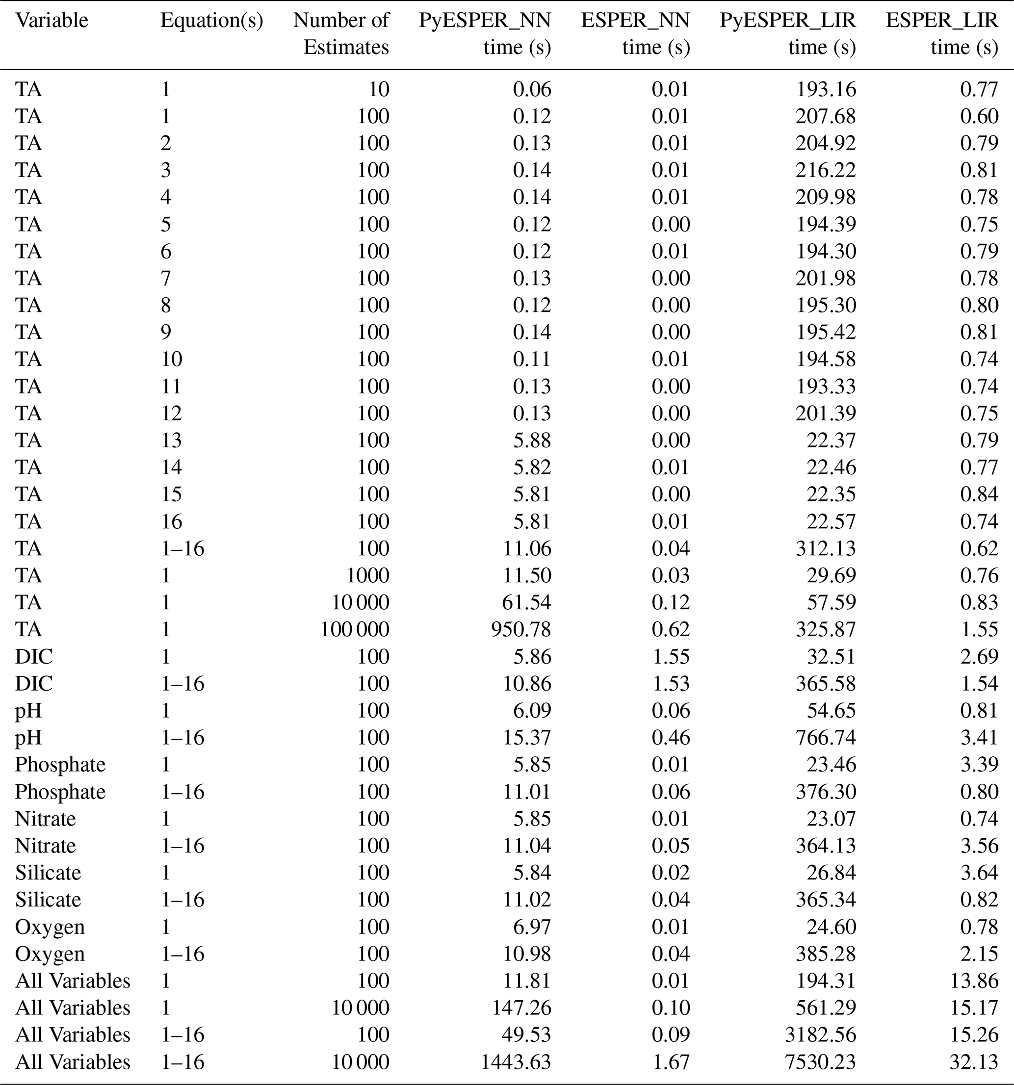
3.2 Speed of calculation

PyESPERs take considerably longer than ESPERs to produce estimates. On a MacBook Air using Python in the terminal with a standard internet connection, PyESPER_NN produced results 0−1500 times slower than ESPER_NN, while PyESPER_LIR produced results about 7−500 times slower than ESPER_LIRs, with the magnitude of the slowdown dependent upon the number of variable inputs and equation cases requested and the number of estimates required (Table 3). ESPER_NNs were the fastest to execute and took <2 s for all time tests, even when large datasets and all variable–equation case scenarios were requested. ESPER_LIRs were the next-fastest, requiring <33 s for all time tests, followed by PyESPER_NNs, which typically required 5–15 s to execute but required >1400 s (23 min) for running large datasets and all variable–equation case scenarios. PyESPER_LIRs were the slowest and typically required 22–500 s to execute, but the longest scenario required 7530 s (125 min; Table 3). It is possible that this code can be further optimized for speed in future updates.

3.3 Future improvements

Updated ESPERs will be trained and assessed using GLODAPv2.2023 (or later versions), which includes 1108 cruises (compared to 946 cruises from GLODAPv2.2020, the current data product used). Additionally, future ESPERs will incorporate depth (z) as an optional predictor variable for consistency with LIPHR, a prior version for estimating pH_T (Carter et al., 2018). The implementation of updated C_ant estimation methods should additionally improve the accuracy and efficiency of both ESPERs and PyESPERs when C_ant estimates are required. Future versions of ESPER written in MATLAB may be modified to improve interoperability with the Python implementation (i.e., to ensure the interpolation routines are identical in all instances between languages).

4 Conclusions

A near-replicate of ESPERs has been produced in the freely available Python programming language. This algorithm data product will offer Python users or researchers with limited funds an alternate, free method for using ESPERs (other than the proprietary MATLAB), increasing the accessibility of the original ESPER algorithms. The same logic applied to the original MATLAB ESPERs was applied within the Python coding language (PyESPERs, version 1.0.0), and the results have demonstrated comparability to the ESPER estimates. Estimates from PyESPER_NNs precisely align with those from ESPER_NNs for all equations and desired outcome variable combinations (Fig. 6), and estimates from these two routines align very closely for all estimates and to within machine precision for all but pH_T and DIC, which exhibit slight differences due to the impacts of interpolating for C_ant. The PyESPER_LIR estimates differ from the ESPER_LIR estimates for some coastal and deep-water regions between the two coding languages due to triangulation, extrapolation, and interpolation differences, but they were more similar throughout all portions of the open ocean (Figs. 2–4). Notably, PyESPER_LIR performs equivalently to ESPER_LIR when reconstructing the training data from GLODAPv2.v2022, so estimates produced from these two routines should be considered comparable rather than identical. Nevertheless, we do not recommend using PyESPER_LIR in coastal or deep (>5500 m) waters when primarily interested in comparing results with those of the MATLAB implementation of ESPER_LIR. Future updates to ESPERs will include updates to PyESPERs, with adjustments to allow for greater consistency and speed.

Appendix A: ESPER specifications

The sets of equations, predictor variables, and measurement uncertainties used in ESPER and PyESPER (adapted from Carter et al., 2021) are shown below.

Table A1 Input predictor variable combinations used for each ESPER equation (adapted from Carter et al., 2021), where S is salinity, T is temperature, and A,B, and C are as defined in Table A2 (below).

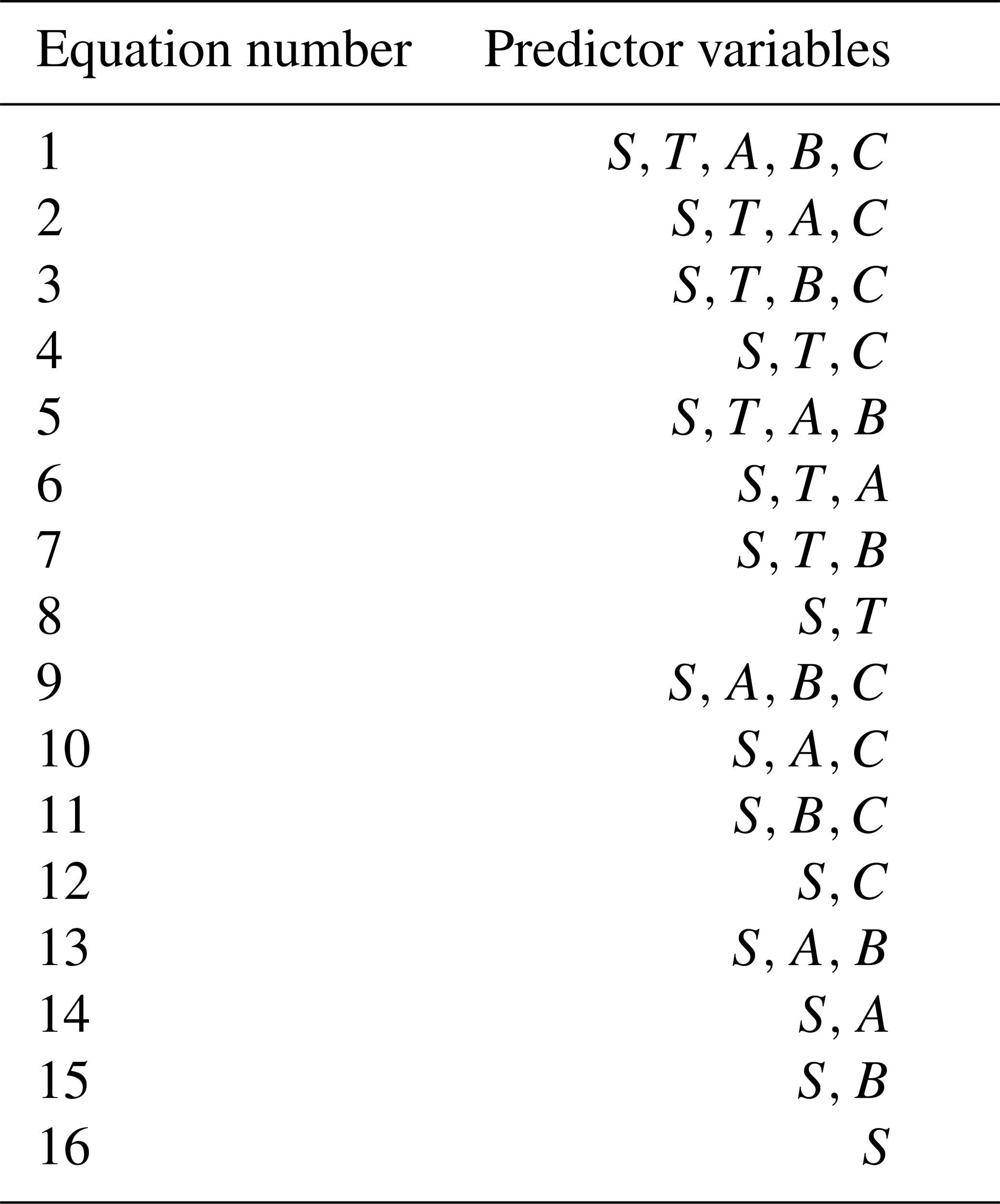
Table A2 Input predictor variables (A,B, and C) for each estimated property (adapted from Carter et al., 2021).

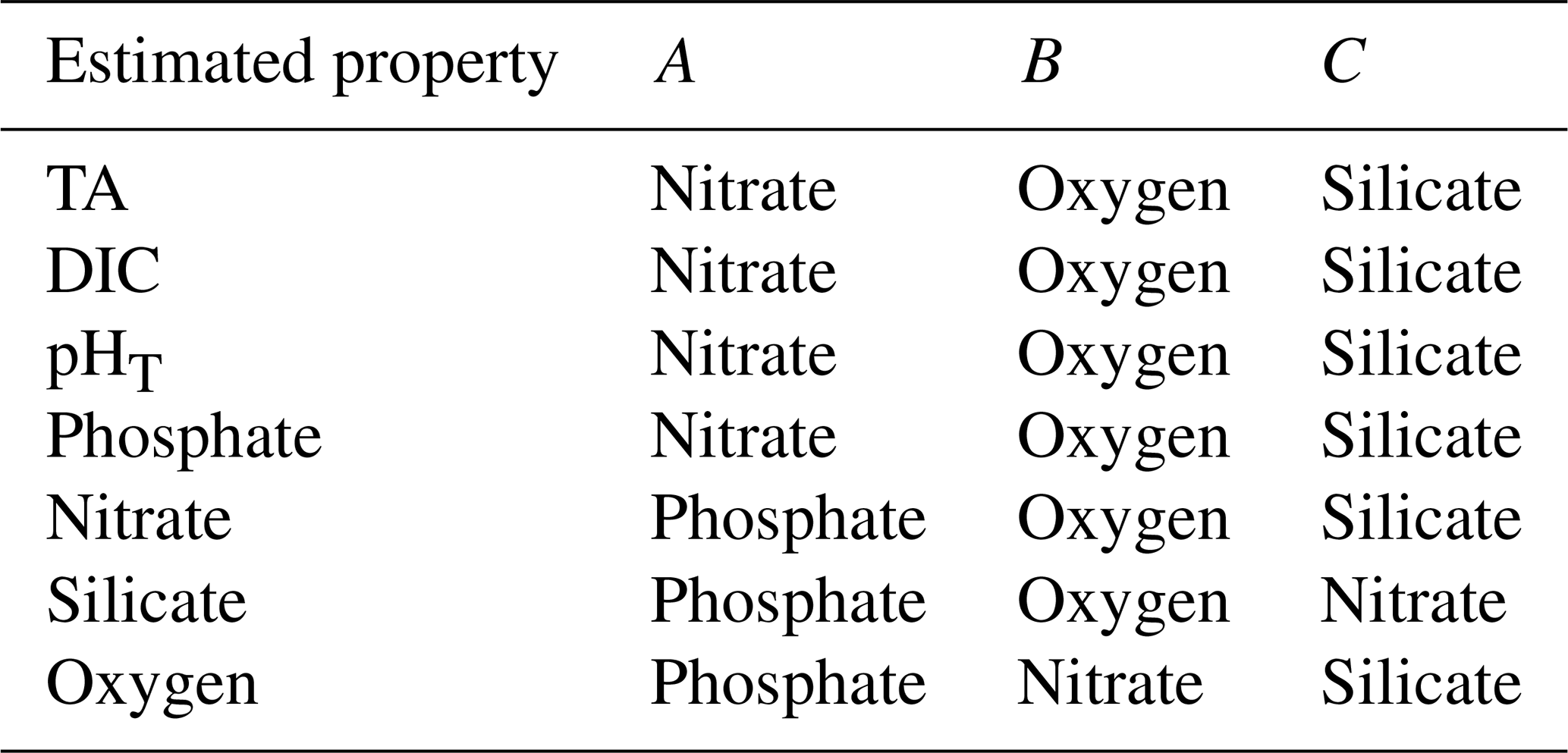
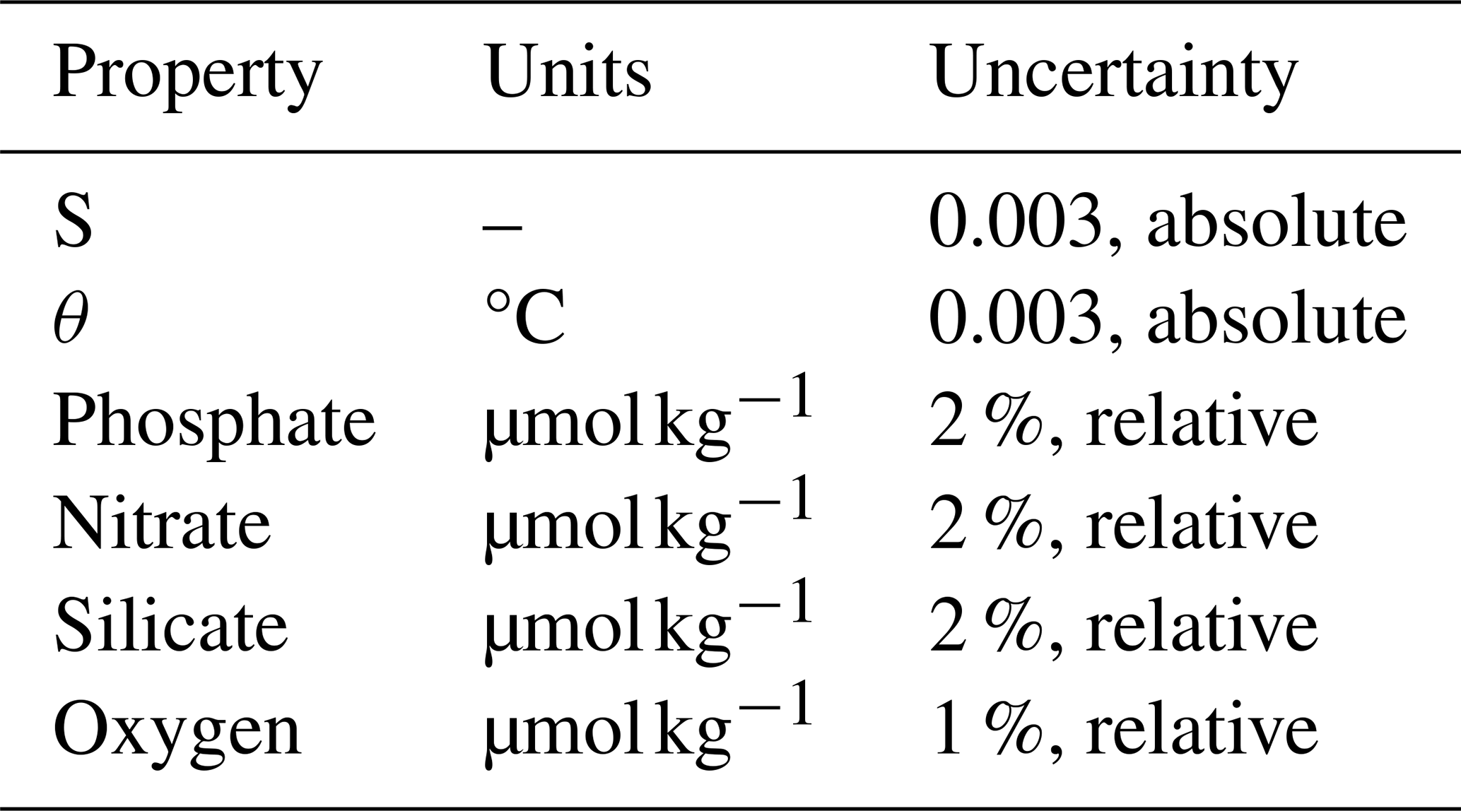
Table A3 Default measurement uncertainties (E_{Pi_Default}) for ESPERs and PyESPERs (adapted from Carter et al., 2021), where θ is the potential temperature.

Appendix B: Comparison using the entire GLODAPv2.2022 dataset

The results of comparisons of PyESPER with ESPER for the entire GLODAPv2.2022 dataset, including the entire oceanic and coastal salinity range and data of all quality control flag categories, are shown below.

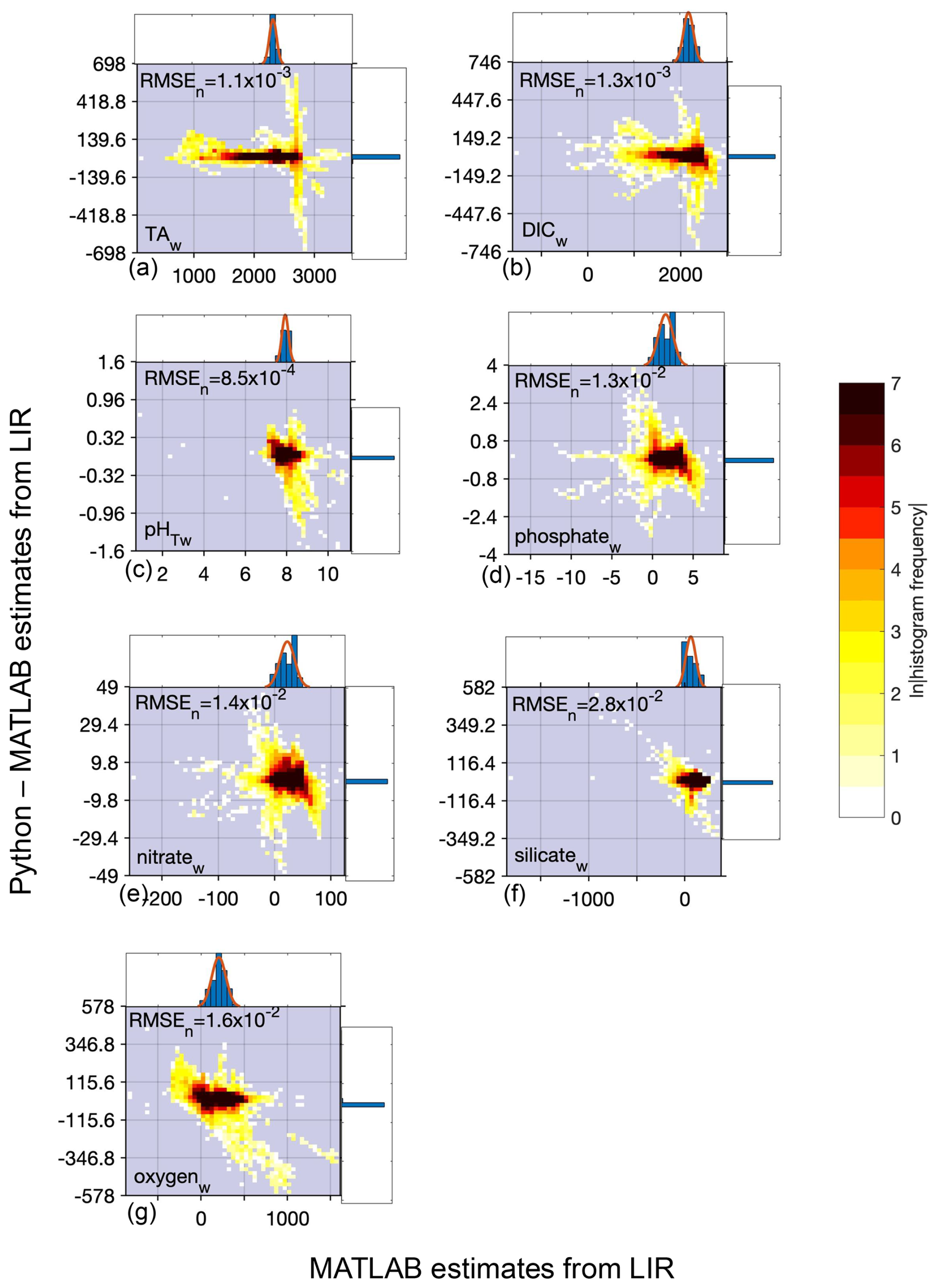
Figure B1 Difference between Python and MATLAB locally interpolated regression estimates (y axis) compared to MATLAB estimates (x axis) for whole ocean (_w) data and all equations combined (22 099 968 total estimates from all equations for each variable) for TA (a), DIC (b), pH_T (c), phosphate (d), nitrate (e), silicate (f), and oxygen (g) derived using all equations and calculated from the entire GLODAPv2.2022 dataset (n=1 381 248). All units, except for pH_T, are µmol kg⁻¹. Top and side histograms represent the distribution of the x and y axes, respectively. Note the differences in the x- and y-axis scales. RMSE_n is the normalized root mean square error, or the RMSE of all estimates divided by the mean of all MATLAB estimates. The large range of sometimes unrealistic estimates along the x axis can be attributed to the anomalous and sometimes erroneous input data used for predictions.

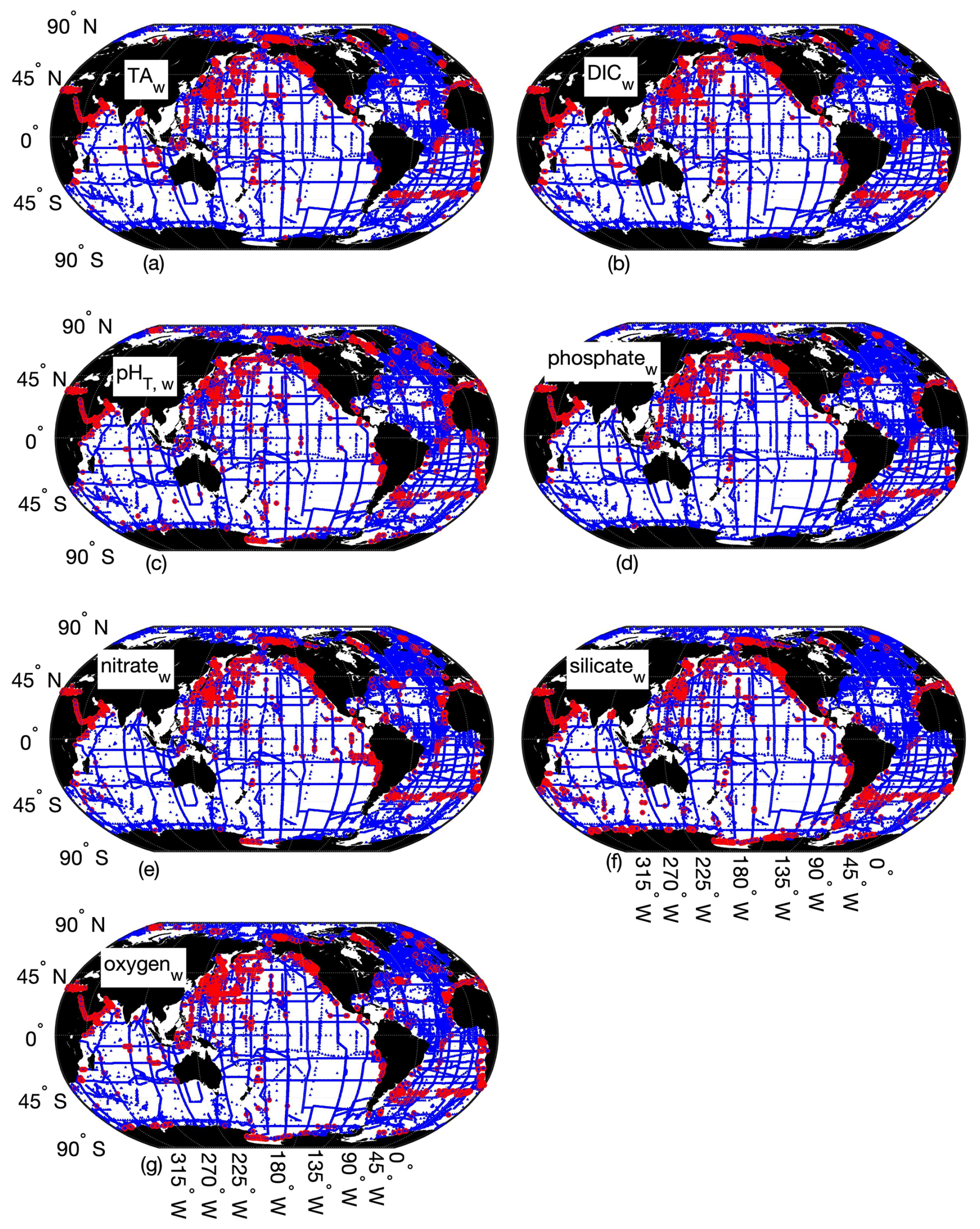
Figure B2 Map of differences between Python and MATLAB ESPER locally interpolated regression estimates (total estimates n=22 099 968 for all variables) for the whole ocean (_w), where the small blue circles represent differences<2 times the uncertainties of the MATLAB estimates (n=22 034 967 for TA (a), 22 054 048 for DIC (b), 22 045 316 for pH_T (c), 22 057 220 for phosphate (d), 22 045 770 for nitrate (e), 22 024 674 for silicate (f), and 22 045 827 for oxygen (g)) and red circles represent differences>2 times the uncertainties of the MATLAB estimates (n=65 001 for TA, 45 920 for DIC, 54 642 for pH, 42 748 for phosphate, 54 198 for nitrate, 75 294 for silicate, and 54 141 for oxygen; n=1 381 248).

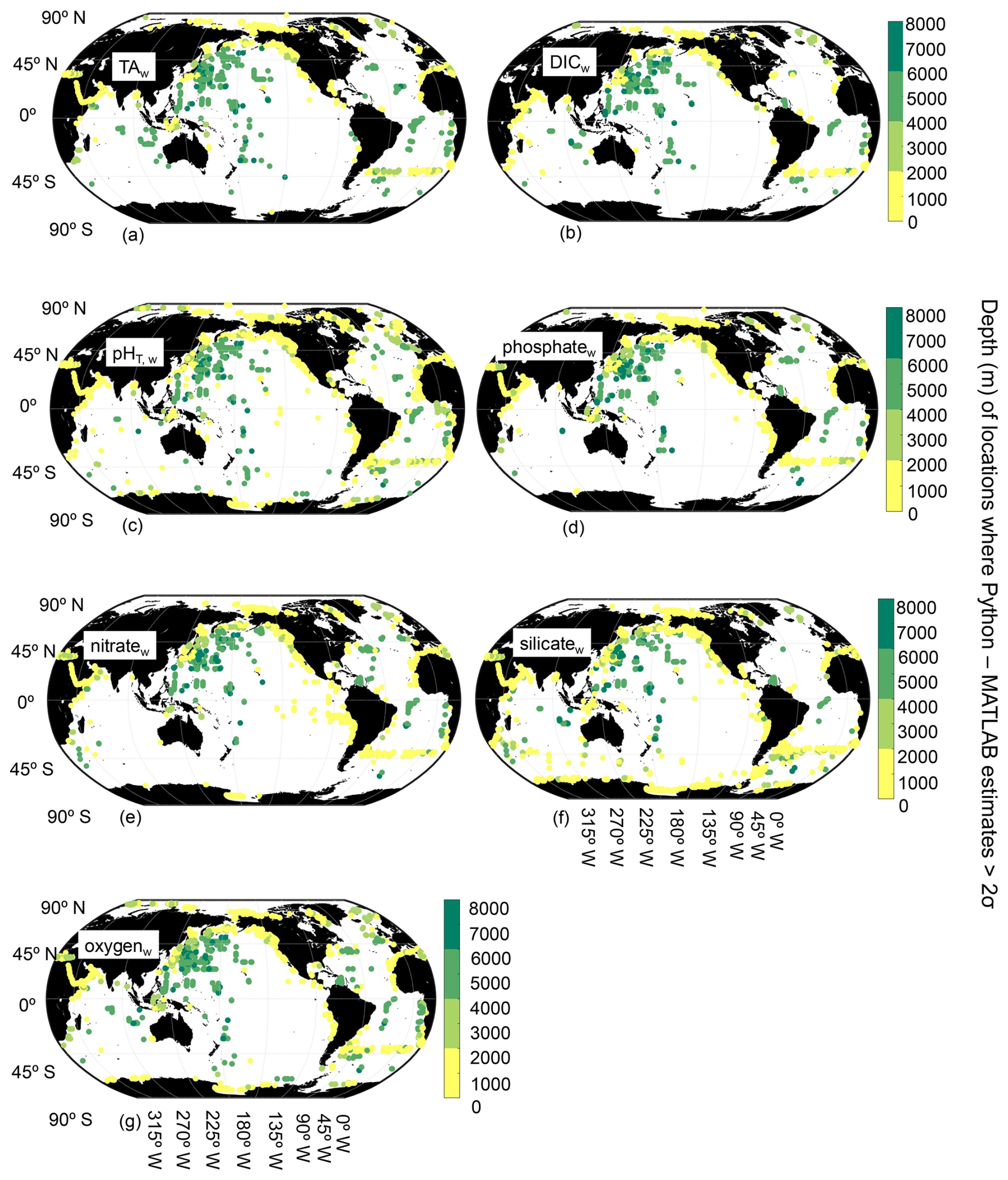
Figure B3 Map of locations and depths (color bar) where the differences between Python and MATLAB ESPER locally interpolated regression estimates are greater than 2 times the estimate uncertainties for the whole ocean (_w, n=22 034 967 for TA (a), 22 054 048 for DIC (b), 22 045 316 for pH_T (c), 22 057 220 for phosphate (d), 22 045 770 for nitrate (e), 22 024 674 for silicate (f), and 22 045 827 for oxygen (g); n=1 381 248).

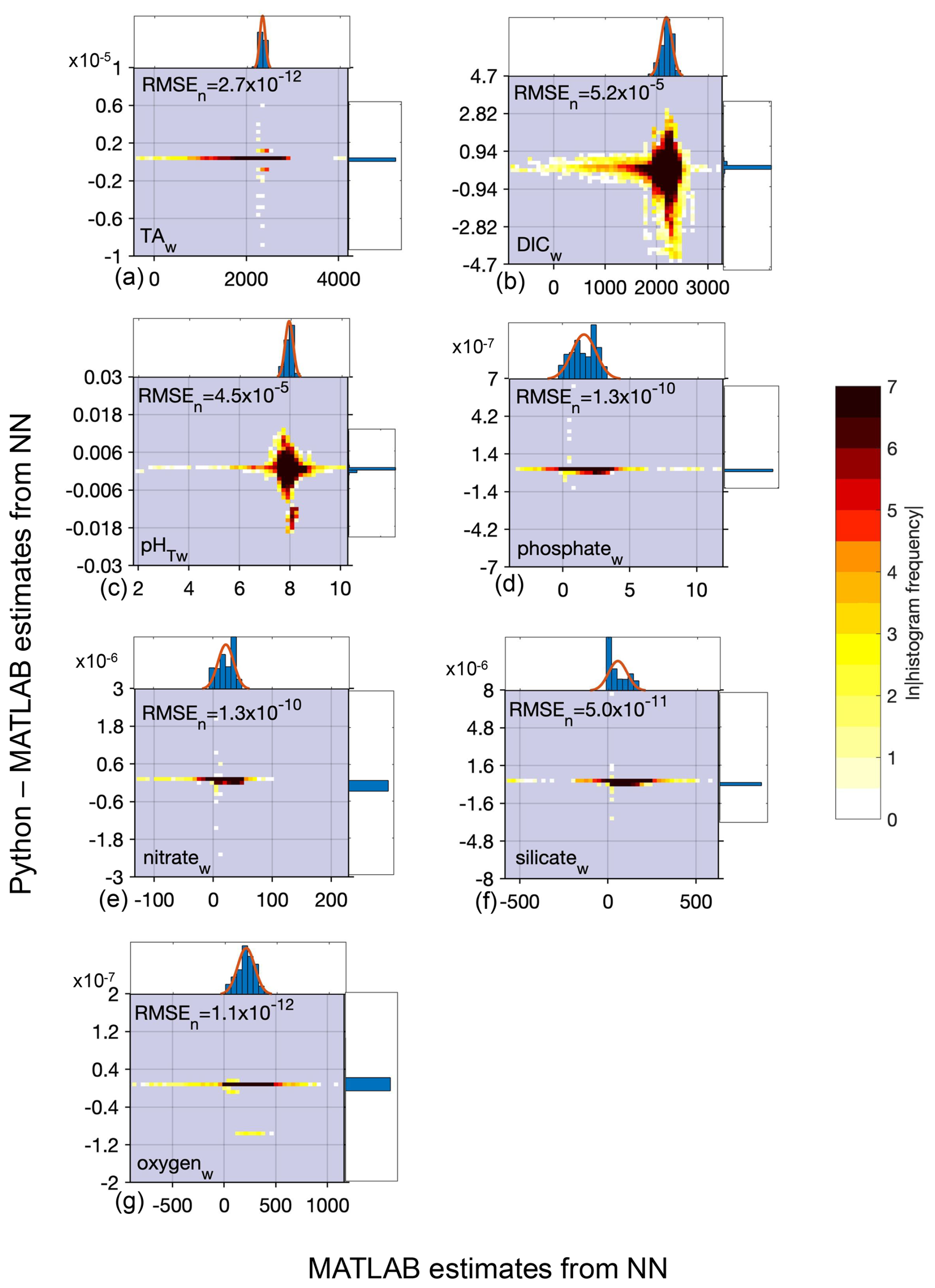
Figure B4 Difference between Python and MATLAB neural network estimates (y axis) compared to MATLAB estimates (x axis) for whole ocean (_w) data and all equations combined for TA (a, 17 802 134 total estimates from all equations), DIC (b, 17 802 134 estimates), pH_T (c, 17 799 566 estimates), phosphate (d, 17 802 134 estimates), nitrate (e, 17 395 954 estimates), silicate (f, 17 445 310 estimates), and oxygen (g, 17 220 360 estimates) derived using all equations and calculated from the entire GLODAPv2.2022 dataset (n=1 381 248). All units, except for pH_T, are µmol kg⁻¹. Top and side histograms represent the distribution of the x and y axes, respectively. Note the differences in the x- and y-axis scales. RMSE_n is the normalized root mean square error, or the RMSE of all estimates divided by the mean of all estimates. The large range of sometimes unrealistic estimates along the x axis can be attributed to the anomalous and sometimes erroneous input data used for predictions.

Table B1 Mean (standard deviation), maximum, minimum, and normalized RMSE (RMSE_n) for differences between MATLAB and Python LIRs, ESPER_LIR and measured values, and PyESPER_LIR and measured values for TA, DIC, pH_T, phosphate, nitrate, silicate, and oxygen estimates (all units, except for pH_T, are µmol kg⁻¹) for all equations combined from the entire GLODAPv2.2022 dataset (_w; n=1 381 248).

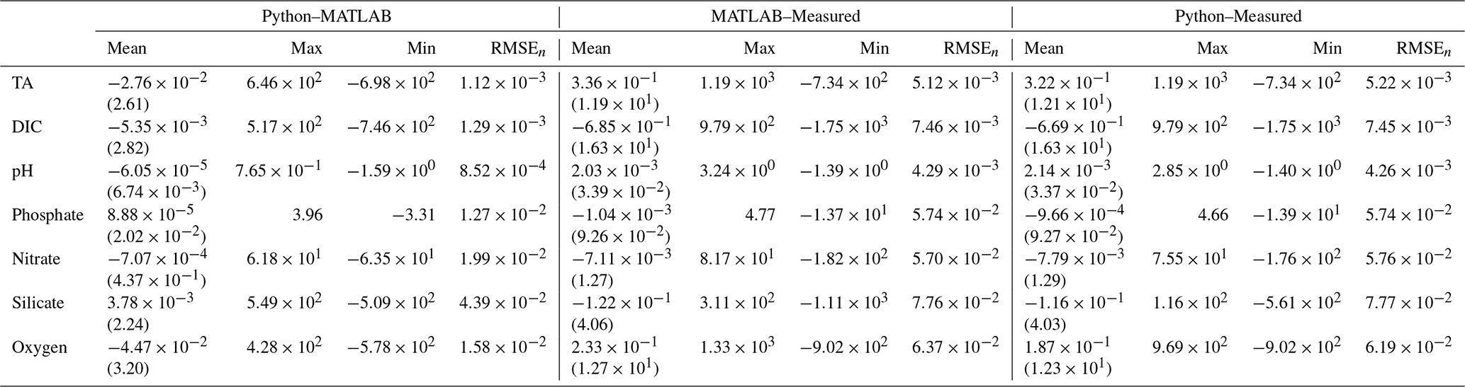
Table B2 Mean (standard deviation), maximum, minimum, and normalized RMSE (RMSE_n) for differences between MATLAB and Python NNs, ESPER_NN and measured values, and PyESPER_NN and measured values for TA, DIC, pH_T, phosphate, nitrate, silicate, and oxygen estimates (all units, except for pH_T, are µmol kg⁻¹) for all equations combined from the entire GLODAPv2.2022 dataset (_w; where necessary input data were available, n=1 381 248).

Appendix C: Example of mapped DIC estimates from PyESPER and ESPER

Surface ocean DIC estimates from PyESPER_LIR and ESPER_LIR were applied to the Roemmich and Gilson climatology (Roemmich and Gilson, 2009). Differences in the surface ocean DIC between the two coding languages (c) illustrate the need to avoid using PyESPER_LIR for DIC in the surface ocean when comparing to MATLAB ESPER_LIR.

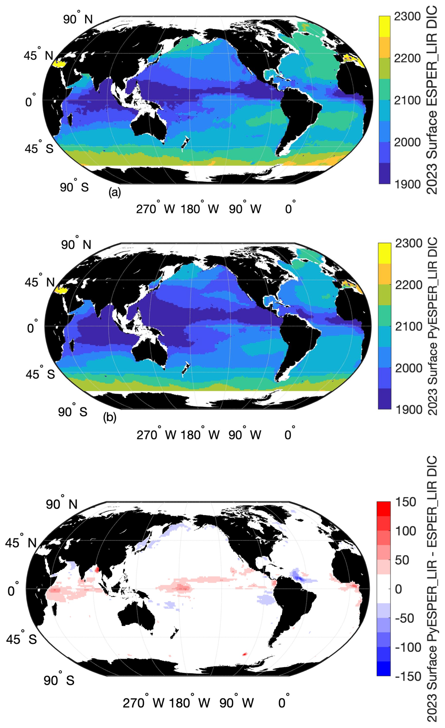
Figure C1 Maps of 2023 mean annual surface estimates of MATLAB ESPER_LIR DIC (a), Python PyESPER_LIR DIC (b), and PyESPER_LIR–ESPER_LIR DIC (c; units are µmol kg⁻¹) from the application of ESPERs to the Roemmich–Gilson Argo (Argo, 2000) climatology (Roemmich and Gilson, 2009).

Appendix D: Comparison of interpolation and extrapolation values between MATLAB and Python

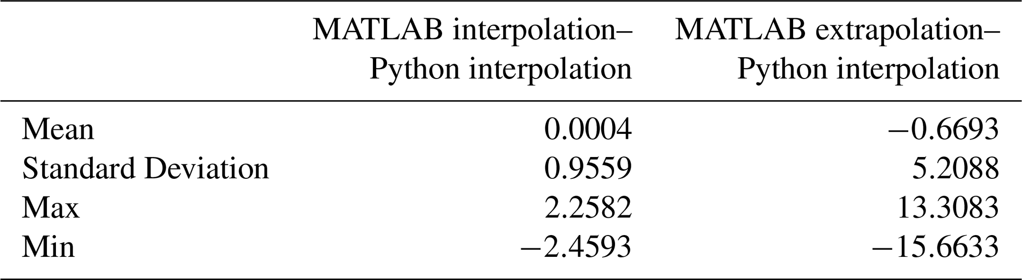
MATLAB ESPER_LIRs avoid extrapolation by addition of a false set of data points at very far distances from the grid. However, when this method was implemented in Python, significant errors were introduced due to the differences in triangulation (which were both valid) between the coding languages. Therefore, it was necessary to find another means of calculating extrapolations in PyESPER_LIRs that was more similar to those of ESPER_LIRs. We did this by producing a larger grid in MATLAB and reading that into Python. A simple demonstration of the errors introduced by this method is described below.

For this comparison, we imagine a hypothetical cube, with x, y, and z coordinates, upon which we wish to provide estimates for a fourth variable (p) via both interpolation and extrapolation (Fig. D1a). We have created a random dataset of points and values within this cube for these demonstration purposes. We then followed the same procedure as in the PyESPER data product creation, whereby we extended this grid in three-dimensional space and used MATLAB scatteredInterpolant extrapolations to estimate values on the expanded grid (Fig. D1b). This method conducts a Delaunay triangulation and then uses both linear interpolation and extrapolation to estimate values. These extrapolated values were then used for interpolation only within Python using SciPy's Delaunay and LinearNDInterpolator functions, which produced more consistent results than interpolation and extrapolation within Python.

When interpolations within Python were compared to locations on the hypothetical grid where interpolations occurred in MATLAB also, the results were more similar than those where the grid was extrapolated within MATLAB. This is because different, but equally valid, mathematics are used to interpolate and extrapolate. Namely, a triangulation is used as the basis for interpolations, whereas extrapolations are based on boundary gradients. Despite these differences, the results were still more similar with this method between the two coding languages than when extrapolations were done in both Python and MATLAB.

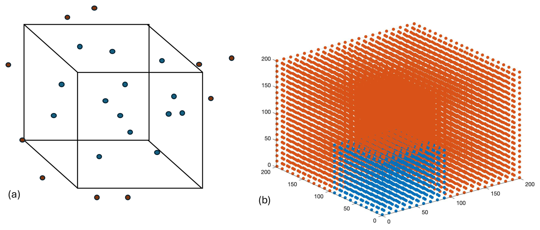
Figure D1 Hypothetical “grid” whereby estimates (p) interpolated within the grid are shown in blue and extrapolations are shown in red (a). Grid created for demonstration purposes, with interpolated values in blue and areas where we extrapolated values in red (b).

Table D1 Comparison of differences between MATLAB interpolations and extrapolations and Python results (all interpolations).