GraphFlow v1.0: approximating groundwater contaminant transport with graph-based methods – an application to fault scenario selection

Groundwater contaminant transport problems remain challenging with respect to their computing requirements. This often limits the exploration of the conceptual uncertainty that is mainly related to large-scale geological features – such as faults, fractures, and stratigraphic variations – and limited characterization. Here, to facilitate geological conceptual uncertainty exploration, we develop further the use of graph representation for geological models to approximate groundwater flow and transport. We consider a faulted multi-heterogeneous-layer medium to test our approach. The existing rank correlation between the shortest path distribution from a contaminant source to the model domain outlet and the cumulative mass distribution at the outlet enables us to perform scenario selection. The scenario selection approach relies on a metric combining the Jaccard dissimilarity and the Wasserstein distance to compare binary images. Among a set combining eight alternative scenarios, where three faults can act as either a flow barrier or a preferential path, we show that the use of graph approximations allows us to retain or reject scenarios with confidence, as well as to estimate the individual probability of a fault to act as a barrier or a path. This methodology framework opens up possibilities to explore more thoroughly conceptual geological uncertainty for processes affected by flow and transport.

1 Introduction

Understanding contaminant transport in subsurface heterogeneous environments is critical to predict pollutant fate and to support effective mitigation strategies. Robust modeling approaches are essential to capture the complexity of these systems and to provide reliable predictions (Bear and Cheng, 2010; Ostad-Ali-Askari and Shayannejad, 2021). Traditional approaches, such as solving partial differential equations (PDEs) for flow and transport, have been extensively used to model groundwater systems (Bear and Cheng, 2010). In particular, MODFLOW 6 is a modeler and solver of differential equations for hydrogeology developed by the US Geological Survey, which is widely used in the research community. However, these methods often require high computational resources (Karmakar et al., 2022), which restrains the exploration of heterogeneity or geological structural uncertainty, such as faults acting as a preferential flow path or a barrier, despite their control on flow and transport conditions.

In recent years, new data-driven approaches have emerged as surrogates for contaminant transport simulation. On the one hand, entirely data-based structures have been developed using various deep learning architectures like transformers (Bai and Tahmasebi, 2022; Pang et al., 2024). On the other hand, there have been recent attempts involving hybrid models like physics-informed neural networks (PINNs), which also include differential equations and boundary conditions as inputs (Meray et al., 2024). In both cases, the results are promising, but the number of simulations required for model training and the lack of transferability remain challenging (Luo et al., 2023). Additionally, tests have mainly been conducted in 1D or 2D due to the significant complexity involved in 3D simulations (Meray et al., 2024).

Graph theory offers a promising alternative to traditional PDE-based models by simplifying the representation of complex systems without the costly training of data-driven methods. For this approach, the first step is to create a graph to represent a geological model. The choice of vertices, edges, and their weights is crucial. Next, an algorithm, often for the calculation of the shortest path or maximum flow, is applied to the graph. In recent years, these graph-based methods have been primarily used for studying fracture networks (Hyman et al., 2018; Karra et al., 2018; O'Ghaffari et al., 2011). In such cases, each intersection between fractures is modeled by a node, and geometric and geological information is stored in the edge weights. The use of graphs is particularly effective for discrete fracture networks (DFNs) due to their high structural complexity, with the number of elements often being too large to be solved by traditional finite-element methods.

Other studies use a graph-based method to approximate the path of minimal hydraulic resistance (or maximal hydraulic conductivity) in a heterogeneous medium. Graphs are generated with hydraulic resistance as weights, and graph algorithms are applied. Mishra et al. (2024) simulate random walks on a 3D graph to approximate CO₂ plume spreading in a reservoir. Both Knudby and Carrera (2006) and Rizzo and de Barros (2017) demonstrate in 2D that shortest-path algorithms approximate quite well the trajectory of the fastest particles in the plume and the drawdown signal.

The objective of this paper is to demonstrate how useful and efficient graph-based approximations of flow and transport can be in reducing geological concept uncertainty in groundwater applications. To do so, we adapt the approach of Rizzo and de Barros (2017), which is limited to a 2D multi-Gaussian heterogeneous medium. Here, we go one step further by integrating general flow direction information and by doing a comparison with flow and transport simulations, thus improving its consistency with subsurface flow and extending its application to a 3D case with increased complexity in terms of heterogeneous aquifer properties by considering a faulted multi-heterogeneous-layer medium. In particular, rather than focusing solely on the best path between the source and a set of target nodes, we calculate the minimal distance between the source and each node, resulting in a distance map. We compare this distance distribution to the distribution of cumulative mass passing through the outlet to evaluate the accuracy of our model. We also assess the robustness of the approximation under the uncertainty of parameters controlling the heterogeneity of subsurface properties. In addition to measuring the performance of this new method for scenario selection, as compared to using more expensive physics-based numerical solvers, we provide a way to predict fault behavior a posteriori based on field measurements.

The paper is organized as follows. The methodology employed is described in Sect. 2. The section starts by introducing the synthetic experimental setting (Sect. 2.1), including a description of the medium heterogeneity and the necessary conditions to numerically solve flow and transport equations. Then, Sect. 2.2 presents how we approximate flow and contaminant transport using distance computation through graphs. Section 2.3 specifies the modalities for observing data from the physics-based model. Section 2.4 introduces metrics to allow the comparison between distance maps from graph computations and cumulative mass maps. Section 2.5 shows to what extent this method can be applied to the selection of fault scenarios. Section 3 presents the general results, highlighting the correlation between the distance distributions and the distribution of cumulative masses, as well as the effectiveness of the method for scenario selection. Finally, the conclusion and the possibilities for future experiments are discussed in Sect. 5.

2 Method

2.1 Experimental setting

For this paper, we consider the following synthetic case, depicted in Fig. 1: a fault zone with three vertical faults and three geological units, each characterized by different heterogeneous property field parameterizations, whose properties are detailed below. The flow propagates primarily in the x direction, with the system's inlet and outlet being maintained at a constant head. A contaminant is continuously injected into approximately the middle of the model, and we study the transport of this contaminant until it exits the model at its outlet face. Flow in a heterogeneous porous medium is modeled using Darcy's law in conjunction with the continuity equation, which, together, describe fluid motion based on the principle of mass conservation. Contaminant transport is modeled using the advection–diffusion equation (ADE), which is based on Darcy's law for advection and Fick's law for diffusion and dispersion. The flow and transport equations are solved using a finite-difference solver, applied on a structured mesh. Faults influence the transport of the contaminant by locally altering the hydraulic conductivity. In this synthetic case, we assume that the faults can either increase or decrease the conductivity by a factor of 100 with respect to the value assigned by the underlying multi-Gaussian field in the absence of faults. As such, faults can act as either a pathway (1) or a barrier (−1). Considering all possibilities, there are eight possible fault scenarios, designated by a triplet $(f_{\mathrm{1}},f_{\mathrm{2}},f_{\mathrm{3}})$ belonging to $\mathit{\{}-\mathrm{1},\mathrm{1}{\mathit{\}}}^{\mathrm{3}}$. The highly schematic geometry of the faults was chosen to maximize the variability of the plume depending on the behavior of the faults. We add further variability by testing 10 possible source positions (Table 1), chosen randomly around a reference point with the coordinates x_s=2000 m, y_s=2500 m, and z_s=512.5 m. This results in a total of 80 scenarios, numbered from 0 to 79, where the tens digit refers to their fault scenario and the units digit refers to the source position.

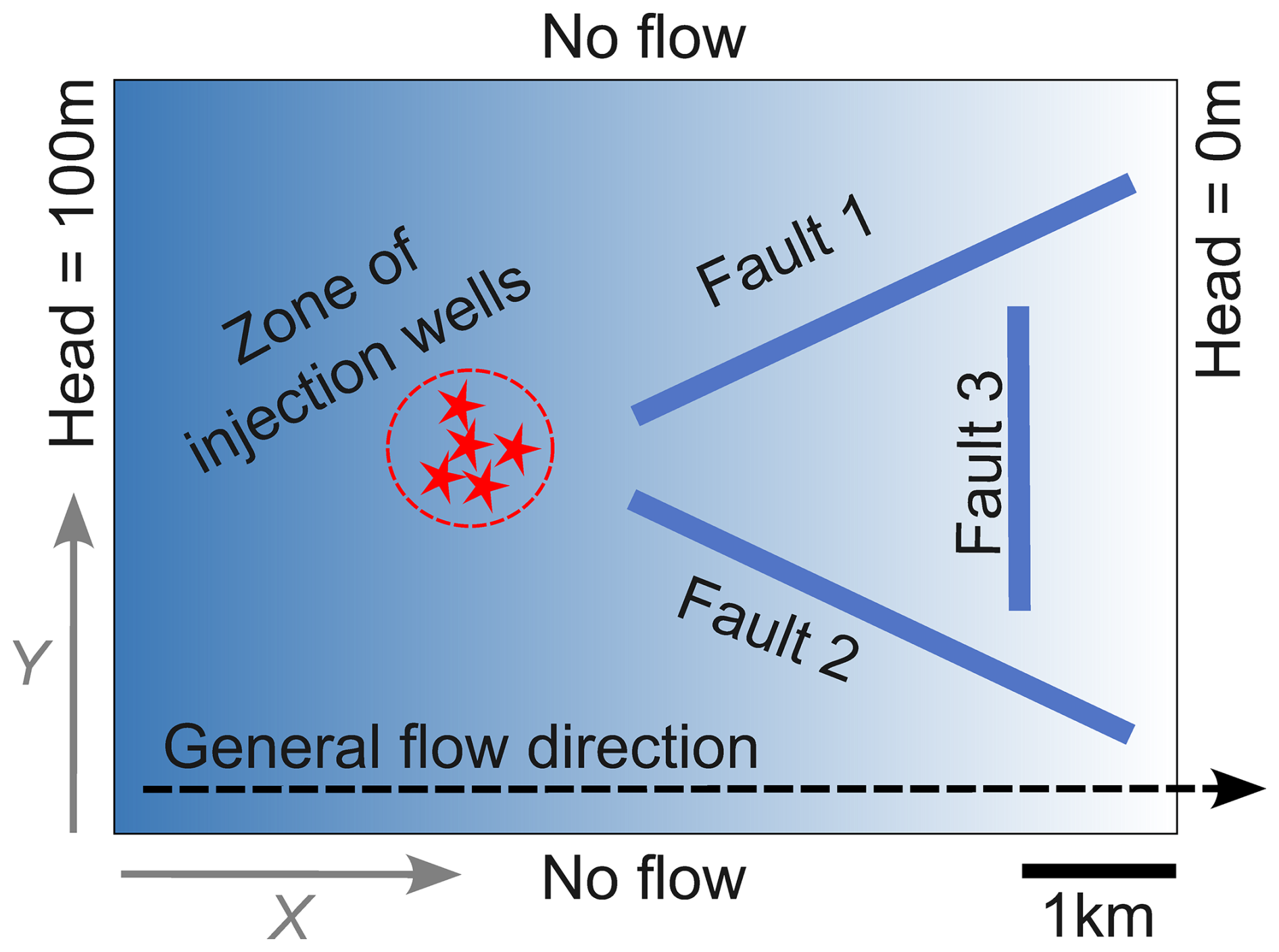
Figure 1 Geometry of the synthetic 3D simulation domain. The domain has dimensions L_x=7000 m, L_y=5000 m, and L_z=1000 m and is discretized with a structured mesh of cell size of Δx=100 m, Δy=100 m, and Δz=25 m. Three vertical fault planes are located within the domain, and they are orthogonal to the x–y plane shown in the figure. These faults can either increase or decrease the local conductivity by a factor of 100, acting, respectively, as pathways or barriers to flow. The figure also illustrates the direction of the main flow (from left to right along the x axis) and the approximate central location of the contaminant injection source, randomly varied within a predefined region across scenarios.

Table 1 Coordinates of the 10 randomly drawn contaminant source positions.

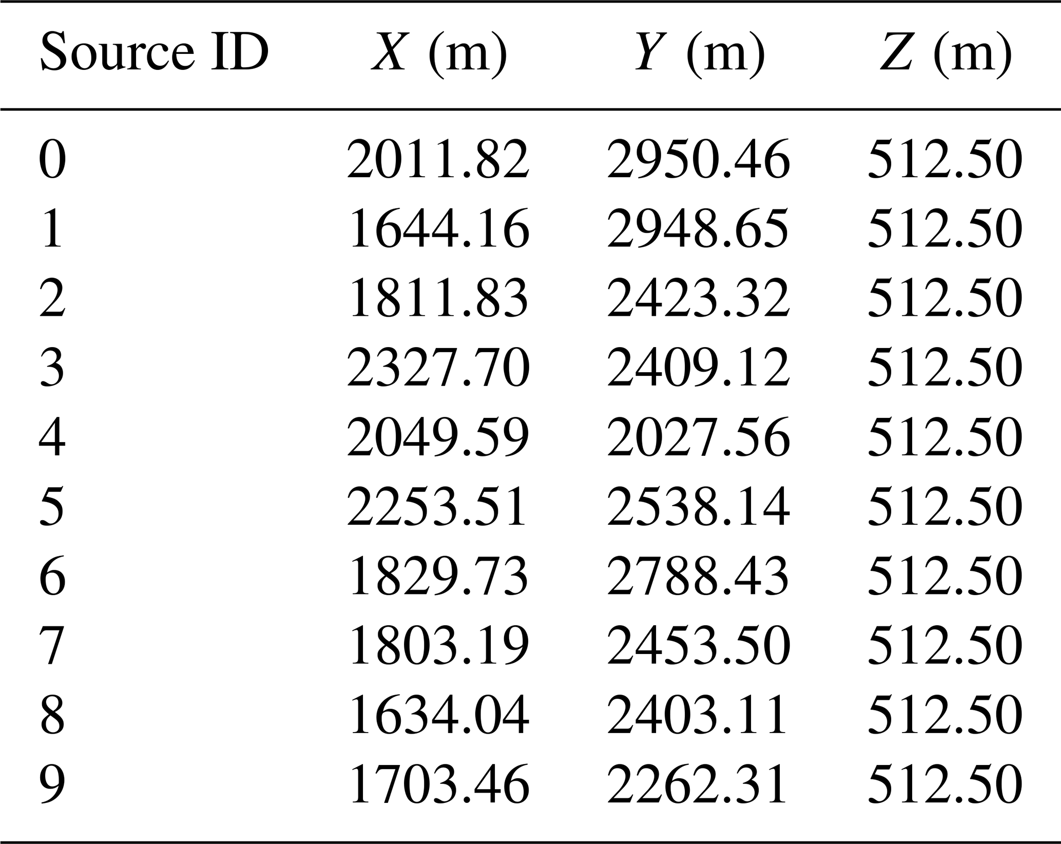
The model dimensions are L_x=7000 m, L_y=5000 m, and L_z=1000 m. Spatial discretization is done in cells of size Δx=100 m, Δy=100 m, and Δz=25 m. The primary direction of flow is along the x axis: the heads at the planes x=0 m and x=7000 m are constant and equal to 100 and 0 m, respectively. The other boundaries of the model are constrained by zero flux. In our study, we assume a point source (one cell) that continuously injects a contaminant at a rate of 50 000 m³ d⁻¹, with a concentration of 100 units of mass per cubic meter (m³). Each scenario is characterized by unique aquifer properties that are produced by combining stochastic property field realizations. The subsurface consists of three geological units with average conductivity of $\mathrm{3.5}\times {\mathrm{10}}^{-\mathrm{5}}$, $\mathrm{8.0}\times {\mathrm{10}}^{-\mathrm{4}}$, and $\mathrm{2.0}\times {\mathrm{10}}^{-\mathrm{5}}$ m s⁻¹, respectively, and constant porosity of 0.25. For each scenario, the hydraulic log conductivity (before the effects of faults) of each geological unit is modeled by a spatial random field (SRF) with a multi-Gaussian (MG) model, with standard deviations of 0.4, 0.5, and 0.6, respectively, and a correlation length of 8Δx, 4Δy, and 2Δz. The faults are modeled directly on the regular-grid voxel so that each fault occupies an ensemble of face-connected voxels in the model. An example of sections of the hydraulic conductivity field is shown in Fig. 2.

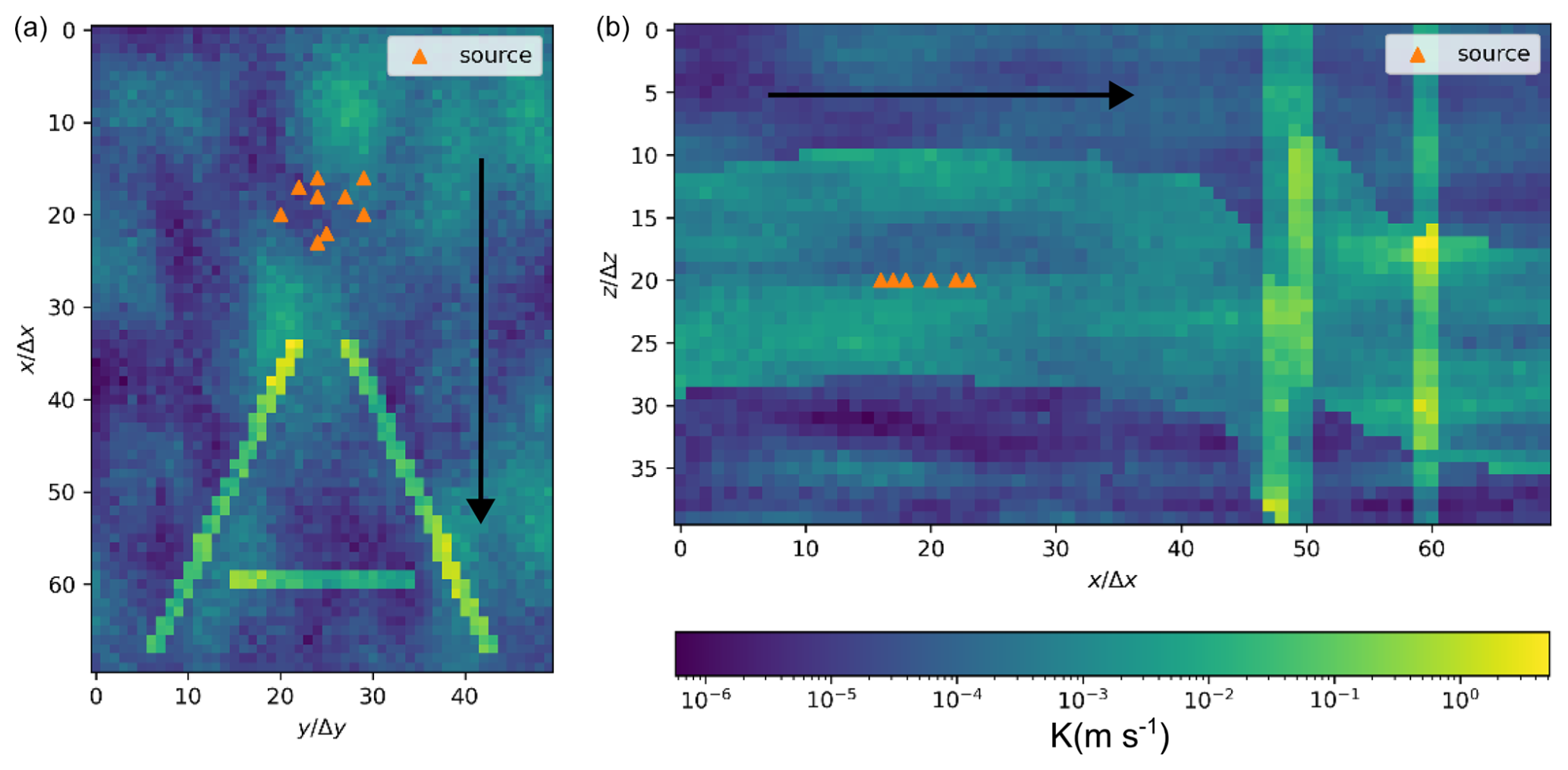
Figure 2 Sections of the hydraulic conductivity field (in m s⁻¹) for the fault scenario $(\mathrm{1},\mathrm{1},\mathrm{1})$, where all three faults act as pathways (i.e., increase conductivity). The hydraulic conductivity field is generated using a multi-Gaussian spatial random field model with heterogeneous geological units. (a) Horizontal section at depth index $z/\mathrm{\Delta }z=\mathrm{30}$. (b) Vertical section at lateral index $y/\mathrm{\Delta }y=\mathrm{15}$. Fault planes are vertical and orthogonal to the x–y plane. The orange dots represent the possible contaminant injection locations. The black arrow indicates the main direction of flow (along the x axis). Axes are labeled in terms of discretization units.

2.2 Graph generation and computation

In order to take advantage of Dijkstra's algorithm to find the shortest paths between graph nodes and to use such a formulation as an approximation for subsurface contaminant flow and transport, the underlying aquifer model has to be represented as a graph. Here, we explain how the regular-grid discretization of an aquifer model can be converted into a graph.

2.2.1 Graph generation

A graph G(V,E) is defined as a pair comprising a set V of vertices and a set E of edges. Each edge e∈E connects two vertices in V and may have an associated weight. In our study, the graphs are directed, and they always have an associated geometric dimension. Thus, for each edge e connecting vertex v₁ to vertex v₂, we use the vector e as the directed vector between the two corresponding points in 3D space. Lastly, a path is described as a sequence of vertices where each pair of consecutive vertices is linked by an edge.

Though the graph is built as an oriented graph, it is similar to a non-oriented graph: all edges are “duplicated” such that, for an oriented edge connecting vertex v₁ to vertex v₂, an oriented edge connecting vertex v₂ to vertex v₁ exists. We use oriented edges as a way to integrate general flow information, such as the main flow direction.

The hydraulic conductivity fields used by physics-based solvers like MODFLOW 6 are discrete fields, which can be defined on both regular and non-regular grids depending on the solver settings. In this work, we focus exclusively on hydraulic conductivity fields defined on regular grids within a bounded 3D space. To construct the graph, we choose the center of each cell in the discrete field mesh as vertices. Two vertices are connected by an edge if their respective cells share a face or a corner.

For an edge e ($[e_x,e_y,e_z]$) connecting two vertices v₁ and v₂, we can calculate an approximation of the hydraulic conductivity tensor K(e) along this edge using the harmonic mean:

$$\begin{array}{}\text{(1)}& \mathbf{K}\left(\mathit{e}\right)=\mathrm{2}\cdot \left(\mathbf{K}\right(v_{\mathrm{1}}{)}^{-\mathrm{1}}+\mathbf{K}(v_{\mathrm{2}}{)}^{-\mathrm{1}}{)}^{-\mathrm{1}},\end{array}$$

where K(v₁) and K(v₂) denote the hydraulic conductivity tensors in the respective cells of vertices v₁ and v₂.

For a given path Γ within 3D space, its hydraulic resistance R_Γ is defined by the following formula (Rizzo and de Barros, 2017):

$$\begin{array}{}\text{(2)}& R_{\mathrm{\Gamma }}=\underset{\mathrm{\Gamma }}{\int }\mathrm{|}{K}^{-\mathrm{1}}\left(l\right)\cdot \mathbf{dl}\mathrm{|},\end{array}$$

with dl being the incremental length along the path Γ.

The concept of hydraulic resistance to groundwater flow is important because the fluid tends to follow paths of minimal resistance (Le Goc et al., 2010). Note also the similarity of this concept compared to that of electrical resistance. We can discretize this definition to apply it to our model. For a given oriented edge e∈E, the hydraulic resistance R_e can be approximated by the following formula:

$$\begin{array}{}\text{(3)}& R_e=\mathrm{|}{\mathbf{K}}^{-\mathrm{1}}\left(\mathit{e}\right)\cdot \mathit{e}\mathrm{|},\end{array}$$

where K(e) is the simplified tensor $[K_{xx},K_{yy},K_{zz}]$ of the hydraulic conductivity on the oriented edge e ($[e_x,e_y,e_z]$).

Rizzo and de Barros (2017) use this value of hydraulic resistance for their modeling. In our case, in 3D and for a point source, we found that the results were more conclusive by adding a corrective factor to this formula in the form of a dot product, preventing paths from going “backwards”. For a given edge e∈E, its weight w_e is defined as follows:

$$\begin{array}{}\text{(4)}& w_e=max({\mathit{f}}_{\text{dir}}\cdot \mathit{e},\mathrm{0})\cdot R_e,\end{array}$$

where f_dir is the main direction of the flow.

To build the graph, we use all cells of the initial model, keep identical information and resolutions, and do not perform upscaling or graph reduction. Thus, we obtain a graph with exactly the same resolution as the original simulation space (as many nodes in the graph as cells in the grid representation), with edge weights that accurately approximate the cost for the contaminant to traverse that edge.

2.2.2 Computation

The shortest-path problem is a classic problem in graph theory. It has several variants, depending on the number of sources and targets and the nature of the weights. In our case, we aim to find the shortest paths between a single source (the contaminant source) and all nodes in the last layer of the model. The algorithm of choice in this case is Dijkstra's algorithm (Dijkstra, 1959). The graph utilized is the one generated in Sect. 2.2.1, with each edge e being assigned the weight w_e from Eq. (4).

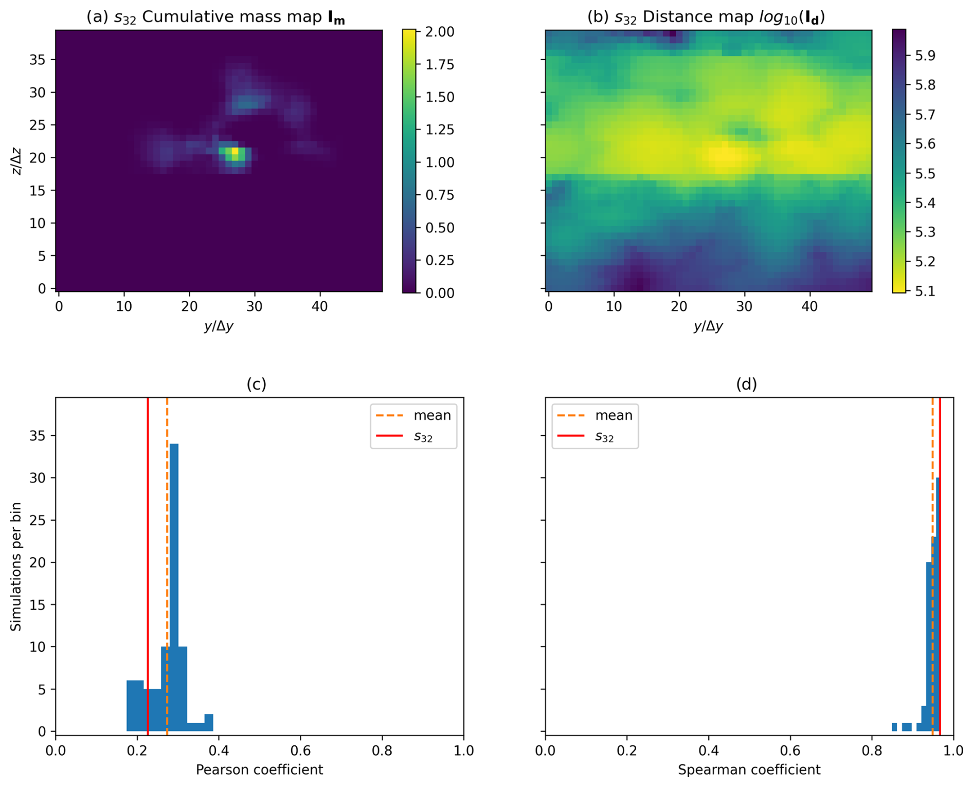
Figure 3 (a) Map of the cumulative mass at FTA for scenario 32. (b) Map of distances between the source and the model outlet face for scenario 32. Both maps are plotted on the outlet face located at x=7000 m using discretized coordinates $y/\mathrm{\Delta }y$ and $z/\mathrm{\Delta }z$. (c, d) Histogram and mean of two correlation coefficients between the negative of the distances and the cumulative mass over all 80 of the scenarios.

Starting from the weighted and directed graph generated in the previous section, we aim to apply a shortest-path algorithm (Dijkstra's algorithm) between the source and the graph nodes corresponding to the model outlet face (for which the hydraulic head is set to 0 m in Fig. 1). Here, the source is a single point, and the model outlet face includes 2000 nodes. Rizzo and de Barros (2017) calculate only the shortest path between the source and the target set. In contrast, we calculate the minimum distance between the source and each node of the model outlet face. This process is not costly because, in general, Dijkstra's algorithm needs to compute all distances to obtain any particular one. We thus obtain a distance value for each vertex in the last layer, resulting in a 2D array that can be visualized as an image. An example is provided in Fig. 3b. In practice, we used the function “get_shortest_paths” from the Python igraph library (Csárdi and Nepusz, 2006), which is compiled in C++. In the following content, the distance map returned by Dijkstra's algorithm is denoted as I_d.

2.3 Observation time

Equivalent simulations were performed with MODFLOW 6 to compare the shortest paths with concentrations calculated numerically. To make the comparison possible, an observation time for the simulation must be chosen. Indeed, while modeling the geological environment as a graph and calculating the shortest paths does not depend on time, the model outlet face concentrations calculated by MODFLOW 6 can vary considerably depending on the chosen observation time. The question is which value should be compared with the values returned by the Dijkstra algorithm and at which observation time. Logically, one can expect that the shortest-path algorithm will better approximate the path taken by the fastest particles of the fluid rather than the slowest ones. Therefore, it seems reasonable to choose a relatively short observation time, a first time of arrival (FTA). Here, we define it as the time in the numerical simulation at the point when the cumulative mass that has passed through the last layer reaches 1 % of the injected mass during the first time step, similarly as in Rizzo and de Barros (2017). For our observations on the last layer of the model, we have chosen to examine the cumulative mass that has passed through it since time t=0 rather than the concentration to be less sensitive to this observation time. An example is given in Fig. 3a. In what follows, the cumulative mass map returned by MODFLOW 6 at FTA is denoted as I_m.

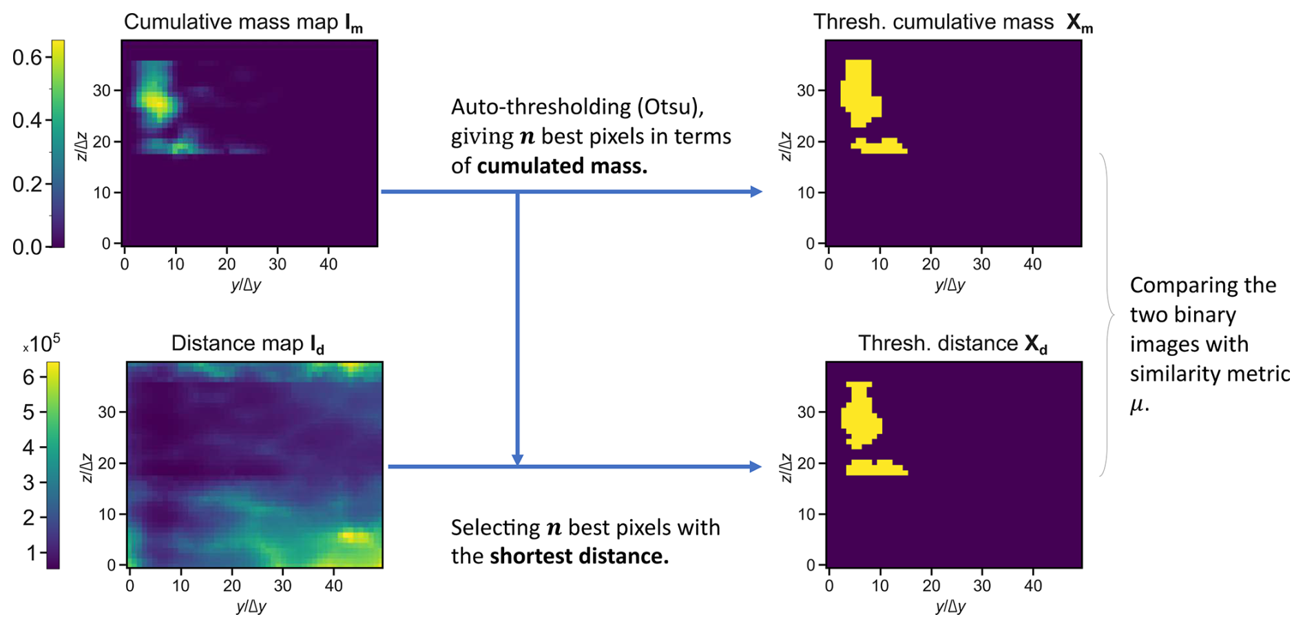
Figure 4 Method to compare cumulative mass and distance maps. The cumulative mass maps are obtained from a numerical solver (in our case, MODFLOW 6), while the distance maps are generated by our model using the shortest path to the outlet, computed with Dijkstra's algorithm.

2.4 Metrics

Comparing briefly the distances map and the cumulative mass map (Fig. 3a and b) over the 80 cases, one can see that the distributions look quite dissimilar. The histograms displaying Pearson and Spearman correlations between the two distributions have been calculated and can be found in Fig. 3c and d. The average values for these correlations are around 0.2 for the Pearson correlation and above 0.9 for the Spearman correlation. This suggests that, while there is a relatively weak correlation between the distributions themselves, the rankings of the pixels exhibit a strong correlation. What interests us more than the correlation between the two entire arrays are the pixels in I_m with significant cumulative mass. The preservation of rank correlation enables us to compare areas displaying high values of cumulative mass with areas displaying the shortest distances, and, thus, we suggest that the proposed proxy is relevant. We want to find a metric that spatially compares the pixels in I_m to the pixels in I_d with low Dijkstra distances. Ideally, given a number n of pixels in I_m displaying the highest values of cumulative mass, for a perfect proxy, the pixels in I_d displaying the n shortest distances would share the same locations in the images. This inspires the following method, represented in Fig. 4:

1. We identify pixels in I_m where the cumulative mass exceeds a certain threshold, denoting them as significant concentration zones, defining a set of n points X_m.

2. The n pixels with the smallest distances are selected in I_d, defining a second set of points X_d.

3. For a certain similarity metric μ, μ(X_m,X_d) is computed.

For step 1, the Otsu thresholding method is utilized (Otsu, 1979). This thresholding method minimizes the intra-class variance for a distribution. It has the strong advantage of being non-parametric and is considered to be a reference in computer graphics. For step 3 of comparing between the two sets of points, the problem is reduced to comparing two binary images, assigning the label 1 to points in the sets of interest and the label 0 to others. Numerous metrics exist in the machine learning literature for segmentation problems. We have chosen to employ two complementary metrics: the Jaccard similarity index and the normalized Wasserstein distance.

The Jaccard index, also known as the IoU (intersection over union) ratio, quantifies the similarity between two finite sample sets A and B as follows:

$$\begin{array}{}\text{(5)}& J(A,B)={\displaystyle \frac{\mathrm{|}A\cap B\mathrm{|}}{\mathrm{|}A\cup B\mathrm{|}}}.\end{array}$$

In our context, the sets in question are the non-zero pixels X_m and X_d from each image. The Jaccard index is beneficial because it evaluates the overlap between the spots in both images and ranges from 0 (indicating total dissimilarity) to 1 (indicating total similarity). However, its limitations, as outlined in Wang et al. (2022), include a predisposition towards larger areas rather than smaller ones. In the latter, a single-pixel error might significantly impact the IoU ratio. Moreover, the index drops to zero with no overlap between the spots, failing to differentiate between various non-overlapping scenarios, including those where a spot's shape remains preserved despite translation.

Another valuable metric is the Wasserstein distance, or the Earth mover distance, derived from optimal transport theory. This measure assesses the dissimilarity between two distributions or densities by calculating the “cost” of transferring matter from one distribution to the other. The Wasserstein distance can vary depending on the underlying distance metric; in our study, we utilize the Euclidean distance, yielding the 2-Wasserstein distance (W₂), which is the square root of the loss from the following optimization problem:

$$\begin{array}{ll}\text{(6)}& {\displaystyle }{W}_{\mathrm{2}}^{\mathrm{2}}(\mathit{a},\mathit{b})=\underset{\mathit{\gamma }\in {\mathbb{R}}_{+}^{l\times n}}{min}& {\displaystyle }\sum _{i,j}{\mathit{\gamma }}_{j,i}\Vert z_i-z_j^{\prime }{\Vert }_{\mathrm{2}}{\displaystyle }\text{s.t. }& {\displaystyle }\mathbf{\Gamma }\mathbf{1}=\mathit{a}\\ {\displaystyle }& {\displaystyle }{\mathbf{\Gamma }}^T\mathbf{1}=\mathit{b}\\ {\displaystyle }& {\displaystyle }\mathbf{\Gamma }\ge \mathrm{0}\\ {\displaystyle }\text{with }& {\displaystyle }\mathbf{\Gamma }=\left({\mathit{\gamma }}_{i,j}\right),\end{array}$$

where a∈ℝⁿ and b∈ℝ^l represent the sample weights or, in other words, the mass distribution to be displaced, and $(z_i{)}_{i\in \mathit{\{}\mathrm{1},\mathrm{\dots },n\mathit{\}}}=(\mathit{\{}{x}_i,y_i\mathit{\}}{)}_{i\in \mathit{\{}\mathrm{1},\mathrm{\dots },n\mathit{\}}}$ and $(z_j^{\prime }{)}_{j\in \mathit{\{}\mathrm{1},\mathrm{\dots },l\mathit{\}}}=(\mathit{\{}{x}_j^{\prime },y_j^{\prime }\mathit{\}}{)}_{j\in \mathit{\{}\mathrm{1},\mathrm{\dots },l\mathit{\}}}$ are the Euclidean coordinates of the points from the two samples, respectively. The solution of the optimization problem $\mathbf{\Gamma }=\left({\mathit{\gamma }}_{i,j}\right)$ is the optimal transport matrix between the two samples.

In our case, we have two binary images, each of which can be interpreted as a 2D uniform distribution over the pixels with a value of 1. Each such pixel is assigned a value of $\mathrm{1}/k$, where k is the number of pixels with a value of 1 in the respective image, ensuring that the distribution is properly normalized. Thus, in Eq. (6), we take $n=l=\left|{\mathbf{X}}_{\mathrm{m}}\right|$ the number of elements of the sets X_m and X_d, and we define the weight vectors as follows:

$${\displaystyle }\mathit{a}=\mathit{b}={\left(\begin{array}{c}\frac{\mathrm{1}}{n}\mathrm{\dots }\frac{\mathrm{1}}{n}\end{array}\right)}^T,$$

with $(z_i{)}_{i\in \mathit{\{}\mathrm{1},\mathrm{\dots },n\mathit{\}}}$ and $(z_i^{\prime }{)}_{i\in \mathit{\{}\mathrm{1},\mathrm{\dots },n\mathit{\}}}$ being the 2D coordinates of the elements of the sets X_m and X_d, respectively.

Directly dealing with this distance can be challenging due to its dependence on the data type, including the sample size and the characteristic distance between samples, and because it does not scale between 0 and 1. An approach, as developed in Wang et al. (2022), introduces the normalized Wasserstein distance (NWD), which scales from 0 (indicating total dissimilarity) to 1 (indicating total similarity):

$$\begin{array}{}\text{(7)}& \text{NWD}({\mathbf{X}}_{\mathrm{m}},{\mathbf{X}}_{\mathrm{d}})=\exp \left(-{\displaystyle \frac{W_{\mathrm{2}}({\mathbf{X}}_{\mathrm{m}},{\mathbf{X}}_{\mathrm{d}})}{C}}\right),\end{array}$$

where C is “a constant closely related to the dataset” (Wang et al., 2022). C is chosen as the average standard deviation of the coordinates of the sets X_m and X_d, calculated across multiple scenarios. The NWD has the advantage of better accounting for results that are merely translated, correlating closely with the distance between the centers of mass of the distributions (Lipp and Vermeesch, 2023), but it has the disadvantage of overly penalizing cases where a dissimilar pixel is very far from the areas of similarity between the two images.

To mitigate this, we have calculated the arithmetic mean of the Jaccard index and the NWD as a similarity index, denoted as μ:

$$\begin{array}{}\text{(8)}& \mathit{\mu }({\mathbf{X}}_{\mathrm{m}},{\mathbf{X}}_{\mathrm{d}})={\displaystyle \frac{\text{NWD}({\mathbf{X}}_{\mathrm{m}},{\mathbf{X}}_{\mathrm{d}})+J({\mathbf{X}}_{\mathrm{m}},{\mathbf{X}}_{\mathrm{d}})}{\mathrm{2}}}.\end{array}$$

Thus, following the method above, we select the pixels of interest in both images I_m and I_d, and we calculate their similarity index using the function μ. Therefore, we define the function μ^*, which performs all of this for the two images I_m and I_d and returns their similarity:

$$\begin{array}{}\text{(9)}& {\mathit{\mu }}^{*}({\mathbf{I}}_{\mathrm{m}},{\mathbf{I}}_{\mathrm{d}})=\mathit{\mu }({\mathbf{X}}_{\mathrm{m}},{\mathbf{X}}_{\mathrm{d}}).\end{array}$$

2.5 Method of scenario selection

Suppose we are dealing with a geological setting where we know the conductivity field and the source position, and we have measurements of the cumulative fluid mass that has traversed the output layer up to the present time. Faults are present, but we are uncertain whether they behave as a preferential path or barrier. Can we predict the nature of these faults using our shortest-path method and our similarity metric μ? To address this question, we aim to compare the similarity between binary images generated from MODFLOW 6 (which we consider to be our ground truth or reference data) and those resulting from the shortest-path calculations, as described in the preceding sections.

For a known source position j and conductivity field, let S_j be the set of fault scenarios, and let n_f=|S| be the number of possible fault scenarios. Let us use, for each scenario s, I_m(s) and I_d(s) as the arrays of, respectively, cumulative mass and distance. Two methods to predict the fault scenario are described in the following sections: one method selects a set of scenarios to reduce uncertainty, while the other assigns a probability to each fault for its behavior.

2.5.1 Scenario selection

We are striving to develop a method to identify, from a discrete set of potential scenarios, which scenario aligns with the actual measurements of cumulative mass in the output layer. However, we have noted that, despite the accuracy of the MODFLOW 6 simulation, certain scenarios lack sufficient variability to be distinguished, especially when the fault that distinguishes them has minimal or no impact on the plume. Thus, given a reference scenario (s₀∈S_j), we aim to devise a strategy (represented by a function f) to select a set f(s₀) of scenarios (instead of one scenario) that includes our reference scenario s₀. Equivalently, this function would reject certain scenarios and thus reduce the uncertainty. This function should rely exclusively on the cumulative mass map I_m(s₀) of s₀ and the set of distance maps from all scenarios $\mathit{\left\{}{\mathbf{I}}_{\mathrm{d}}\right(s),s\in S_j\mathit{\}}$. Ideally, we would like to find a function satisfying f(s)={s} for every scenario s, but, as we said, this is not always possible due to the low inter-scenario variability of the model and the approximations of our method based on shortest paths.

Thus, we define the success of a strategy f applied to scenario s, denoted as Y(f,s):

$$\begin{array}{}\text{(10)}& Y(f,s)={\mathbb{1}}_{\mathit{\{}s\in f(s\left)\mathit{\right\}}},\end{array}$$

returning 1 if s∈f(s) and returning 0 otherwise. We also define w(f,s) – that, is the number of scenarios selected by the strategy f for the scenario s:

$$\begin{array}{}\text{(11)}& w(f,s)=\mathrm{|}f\left(s\right)\mathrm{|}.\end{array}$$

From these results, we can calculate, for a strategy f, the success rate $\stackrel{\mathrm{‾}}{Y}\left(f\right)$ and the average number $\stackrel{\mathrm{‾}}{w}\left(f\right)$ over all 80 available scenarios (for all possible sources). We would like to maximize the success rate while keeping the average number of selected scenarios low enough to reject the maximum number of scenarios. Therefore, we seek a strategy with the highest possible ratio $\frac{\stackrel{\mathrm{‾}}{Y}\left(f\right)}{\stackrel{\mathrm{‾}}{w}\left(f\right)}$.

We may simply consider the strategy h_k for $k\in \mathit{\{}\mathrm{1},\mathrm{\dots },n_f\mathit{\}}$, which always randomly selects a subset S of size k. For this type of strategy, we obtain a linear response: $\stackrel{\mathrm{‾}}{Y}\left(h_k\right)=\frac{k}{n_f}$ and $\stackrel{\mathrm{‾}}{w}\left(s\right)=k$. This dummy strategy serves as a baseline for improvement; a good strategy should display a metric above this linear response.

An idea for a method is for a certain threshold $\mathit{\lambda }\in [\mathrm{0},\mathrm{1}]$ to retain only the scenarios (s_i) such that ${\mathit{\mu }}^{*}\left({\mathbf{I}}_{\mathrm{m}}\right(s),{\mathbf{I}}_{\mathrm{d}}(s_i\left)\right)\ge \mathit{\lambda }$. We thus define the strategy g_λ for $\mathit{\lambda }\in [\mathrm{0},\mathrm{1}]$:

$$\begin{array}{}\text{(12)}& g_{\mathit{\lambda }}\left(s\right)=\mathit{\{}t\in S_j,{\mathit{\mu }}^{*}({\mathbf{I}}_{\mathrm{m}}\left(s\right),{\mathbf{I}}_{\mathrm{d}}\left(t\right))\ge \mathit{\lambda }\mathit{\}}.\end{array}$$

Another idea is to select all of the scenarios with maximum similarity I. This defines the u strategy:

$$\begin{array}{}\text{(13)}& u\left(s\right)=\underset{j\in S_j}{\text{argmax}}\left({\mathit{\mu }}^{*}\right({\mathbf{I}}_{\mathrm{m}}\left(s\right),{\mathbf{I}}_{\mathrm{d}}\left(j\right)\left)\right).\end{array}$$

2.5.2 Prediction of each fault's behavior

Another way to learn more about the reference scenario is to attempt to predict the behavior of each individual fault rather than directly seeking to identify the correct scenario. For a given reference scenario s₀, we want to calculate a value interpreted as a similarity to predict the behavior of its fault i ($i\in \mathit{\{}\mathrm{1},\mathrm{2},\mathrm{3}\mathit{\}}$ in our example). For a given scenario s₀, we define the binary value F_i(s₀), which equals 1 if fault i is a preferential path in scenario s₀ and −1 if it is a barrier.

The sum of similarities between the reference scenario s₀ and the scenarios where the fault i behaves as a path divided by the sum of similarities to the reference scenario for all scenarios returns a value between 0 and 1 that can be interpreted as a probability:

$$\begin{array}{}\text{(14)}& P\left(F_i\right(s_{\mathrm{0}})=\mathrm{1})={\displaystyle \frac{{\sum }_{s\in S_j,F_i\left(s\right)=\mathrm{1}}{\mathit{\mu }}^{*}\left({\mathbf{I}}_{\mathrm{m}}\right(s_{\mathrm{0}}),{\mathbf{I}}_{\mathrm{d}}(s\left)\right)}{{\sum }_{s\in S_j}{\mathit{\mu }}^{*}\left({\mathbf{I}}_{\mathrm{m}}\right(s_{\mathrm{0}}),{\mathbf{I}}_{\mathrm{d}}(s\left)\right)}}.\end{array}$$

Indeed, this ranges from 0 (if s₀ is very dissimilar to the scenarios with i as a preferential path) to 1 (if s₀ is very similar to these scenarios). Similarly, the probability for the fault i to behave as a barrier for scenario s₀ can be seen as this normalized sum:

$$\begin{array}{ll}{\displaystyle }P\left(F_i\right(s_{\mathrm{0}})=-\mathrm{1})& {\displaystyle }={\displaystyle \frac{{\sum }_{s\in S_j,F_i\left(s\right)=-\mathrm{1}}{\mathit{\mu }}^{*}\left({\mathbf{I}}_{\mathrm{m}}\right(s_{\mathrm{0}}),{\mathbf{I}}_{\mathrm{d}}(s\left)\right)}{{\sum }_{s\in S_j}{\mathit{\mu }}^{*}\left({\mathbf{I}}_{\mathrm{m}}\right(s_{\mathrm{0}}),{\mathbf{I}}_{\mathrm{d}}(s\left)\right)}}\\ \text{(15)}& {\displaystyle }& {\displaystyle }=\mathrm{1}-P\left(F_i\right(s_{\mathrm{0}})=\mathrm{1}).\end{array}$$

This value ranges from 0 and 1 as well, allowing it to be interpreted as a probability. This enables us to predict the behavior of the fault by rounding it to 0 or 1.

3 Results

3.1 General graph approximation performances

The similarity index described in Sect. 2.4 has been applied to analyze the results of the 80 scenarios. For each scenario, a MODFLOW 6 simulation is run to obtain the cumulative mass, a graph calculation is performed to obtain a distance map, and the two outputs are compared via the similarity index. A representative sample of the results can be found in Fig. 5, and the distribution of similarities is shown in Fig. 6. The mean and median similarity over all scenarios are, respectively, 0.62 and 0.74.

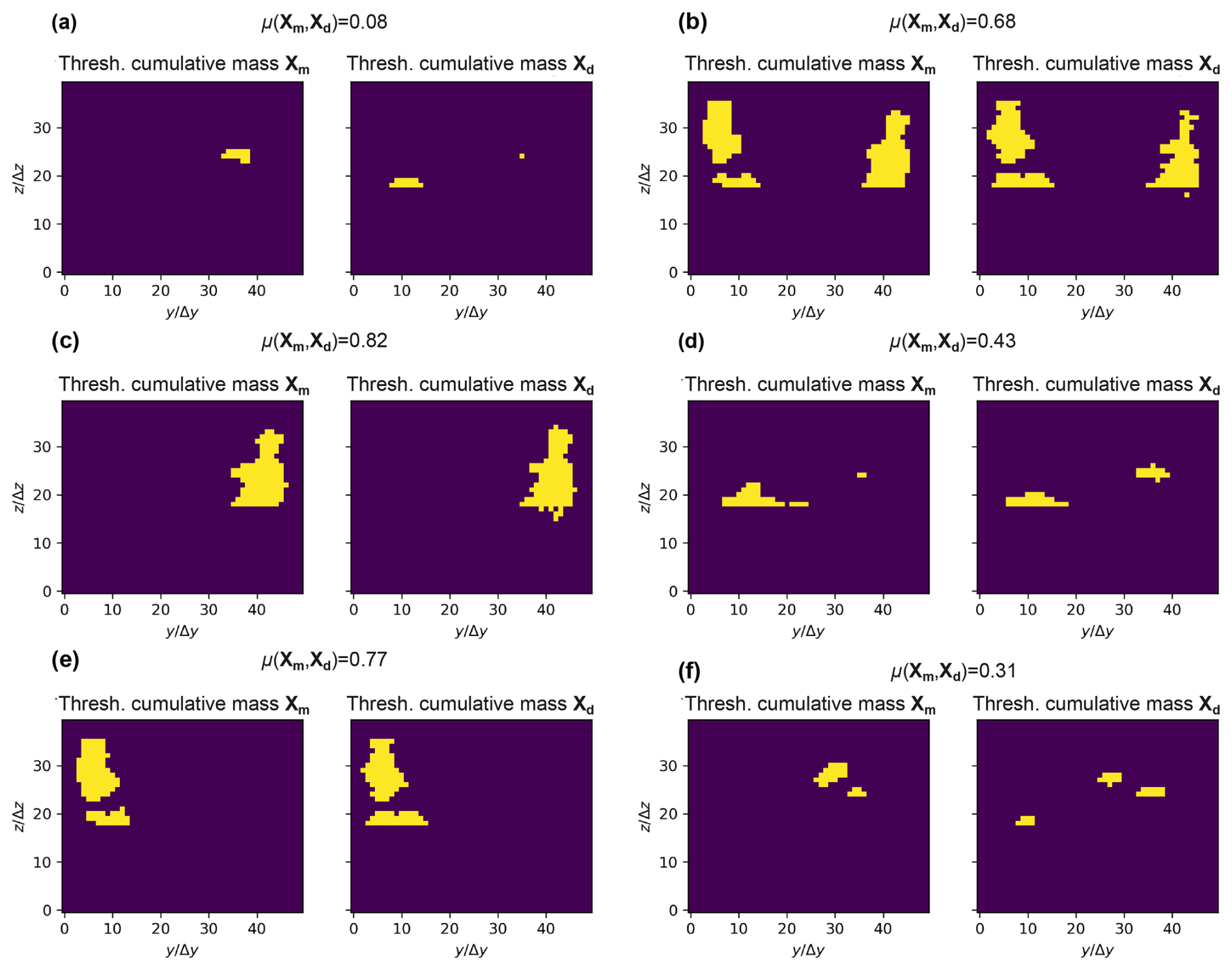
Figure 5 Computation of the similarity for scenarios 0 (a), 76 (b), 36 (c), 8 (d), 27 (e), and 10 (f). For each case, on the left side is the cumulative mass (X_m) at FTA from MODFLOW 6 to which an Otsu thresholding is applied. On the right side, the map of distances (X_d) is shown, thresholded with the same number of pixels as for the cumulated mass map. The similarity values are shown on the top of each figure. The axes are expressed in discretization units.

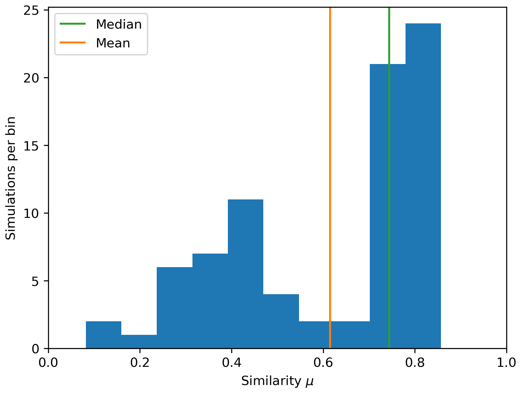
Figure 6 Histogram of similarity index values computed over all 80 scenarios using the similarity formula from Eq. (9). For each scenario, the similarity was calculated between the cumulative mass map at FTA and the corresponding distance maps.

The similarity value is indicative since it was constructed from two different measures and thus requires some interpretation to decide whether or not the approximation is “good enough”. Across all results, we observe that the approximation of X_m by X_d is acceptable when the similarity value is greater than 0.3. Note that what can be considered to be a valid threshold for a good approximation is subject to the user appreciation. If the user is more demanding then they can choose a higher threshold, such as 0.4 or 0.5. In the case of Fig. 5f, we observe that our method captures two out of the three cumulative mass patches present in the MODFLOW 6 simulation and produces a similarity index of 0.31. We can conclude that the distance map provides a good indication of where the cumulative mass will be significantly present.

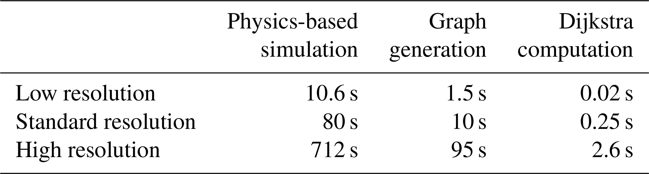
Another important result is the comparison of the computational time between the graph-based method and the physics-based method. We conducted our calculations using our model, as well as two others with coarser (low resolution) and finer (high resolution) resolutions. For the low resolution, the discretization parameters Δx, Δy, and Δz are multiplied by 2, and these are divided by 2 for the high resolution, resulting in the cell volume being either multiplied by or divided by 8. The computation times are presented in Table 2. We observe that, for the method using graphs, generating the graph has a significantly higher cost than calculating the paths. Moreover, the graph generation followed by Dijkstra's calculation takes approximately 10 times less computational time than the MODFLOW 6 simulation.

Table 2 Duration of each simulation for three different model resolutions. The physics-based simulation is conducted with MODFLOW 6, and the graph-based one is conducted with the igraph library.

Figure 7 Cross-similarity between the cumulative mass map at FTA of scenario 65 and the distance maps of all scenarios in S₅ (a) and between the cumulative mass map at FTA of scenario 12 and the distance maps of all scenarios in S₂ (b), computed using the similarity formula from Eq. (9).

3.2 Scenario selection illustration using two examples

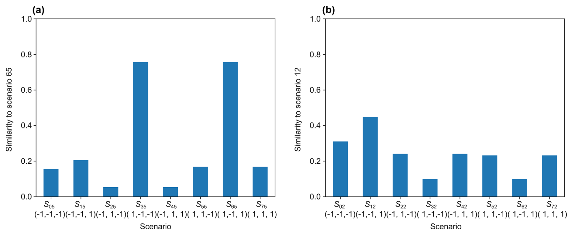
To illustrate the previous methods in a concrete case, we choose scenario number 65 from our database (denoted as s₆₅), which has the source position 5 and corresponds to the fault scenario triplet $(\mathrm{1},-\mathrm{1},\mathrm{1})$ (i.e., faults 1 and 3 are paths, and fault 2 is a barrier). Figure 7 shows the similarity between the cumulative mass map I_m(s₆₅) and each of the distance maps from all fault scenarios ${\mathbf{I}}_{\mathrm{d}}\left(s\right),s\in S_{\mathrm{5}}$. We can see that two fault scenarios stand out distinctly, namely fault scenarios $(\mathrm{1},-\mathrm{1},-\mathrm{1})$ and $(\mathrm{1},-\mathrm{1},\mathrm{1})$, which include the correct scenario. Indeed, when fault 1 acts as a preferential path and fault 2 as a barrier, most of the flow goes through fault 1, which reaches the model outlet independently of fault 3 (that could act as either a barrier or a preferential path). This means that fault 3 does not influence the shortest path through the graph. Therefore, with the strategies defined in Sect. 2.5.1, namely g_λ (with any threshold between 0.2 and 0.75), or with the strategy u, we can clearly isolate these two scenarios from the rest, allowing us to reject six out of eight fault scenarios. If we attempt to predict the faults individually (as in Sect. 2.5.2), we obtain the probabilities in the second row of Table 3. The prediction is accurate for faults 1 and 2, but, for fault 3, the probability is very close to 0.5, not allowing any conclusion. For scenario 65, we see that both approaches allow for the clear identification of the nature of two out of three faults.

Table 3 Probabilities P(F_i(s)=1) of each fault being a preferential path for scenario 12 and scenario 65.

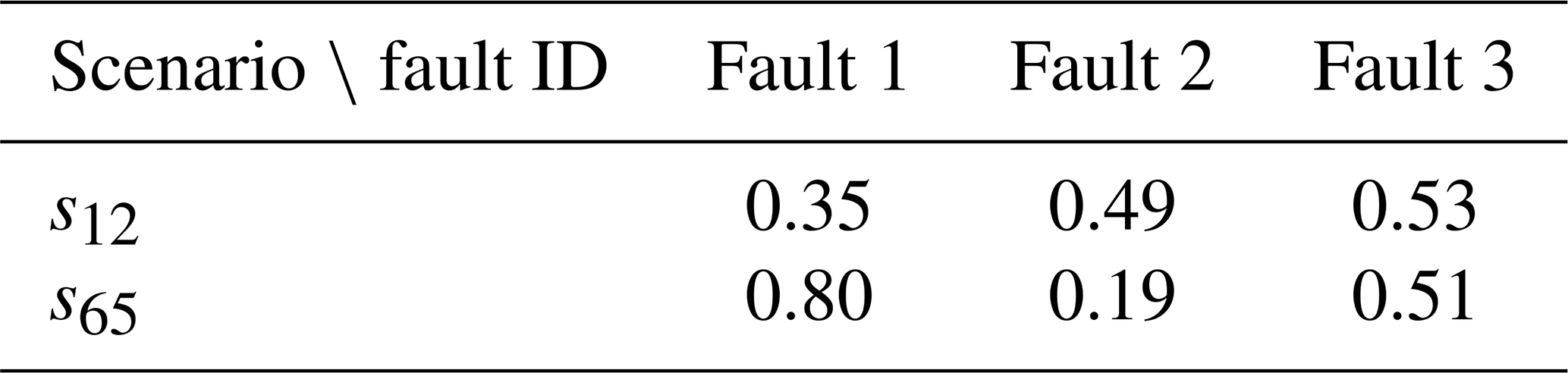
Now, let us consider scenario s₁₂ from our database, which has the source position 2 and corresponds to the fault scenario $(-\mathrm{1},-\mathrm{1},\mathrm{1})$. Looking at Fig. 7, which shows the similarity between the cumulative mass map I_m(s₁₂) and each of the distance maps from all fault scenarios ${\mathbf{I}}_{\mathrm{d}}\left(s\right),s\in S_{\mathrm{2}}$, we can see that it is less clear here. Even if the correct fault scenario has the highest cross-similarity, the difference compared to the others is not substantial enough to make a confident prediction. Using the second method and looking at each fault individually, we obtain the probabilities in third row of Table 3. While the prediction for the first fault is clearly predicted (correctly) to behave as a path, the prediction is poor for faults 2 and 3, with probabilities slightly below or above 0.5. Thus, for this scenario, the results are less favorable, with only one fault being confidently identified.

3.3 Scenario selection overall results

The results of the average success rate $\stackrel{\mathrm{‾}}{Y}$, computed over pairs (80) of fault scenarios (8) and contaminant sources (10), as a function of the average number of selected scenarios $\stackrel{\mathrm{‾}}{w}$, are presented in Fig. 8. It is evident that all data points lie significantly above the baseline curve of the h_k functions. Specifically, selecting the g_λ function for λ=0.5 yields a precision of $\stackrel{\mathrm{‾}}{Y}=\mathrm{0.8}$ and an average number of selected scenarios $\stackrel{\mathrm{‾}}{w}=\mathrm{2}$, which can be interpreted to be a confidence of 80 % to select the right scenario when selecting the two best scenarios. Close results are obtained with the u function. This shows that, with this method, we are able to confidently reject a good portion of the scenarios. Using the probabilities calculated in Eq. (14), we can then calculate the recall and precision for each fault in predicting its behavior. Because there are two possible classes (barrier or path), recall and precision are calculated for both classes. The results are shown in Fig. 9 with blue markers. Additionally, in Fig. 9, the recall and precision scores obtained using the cumulative mass results from MODFLOW 6 from start to finish are shown with orange markers. The fact that the precision and recall are not equal to 1 demonstrates the inherent lack of variability in the data; i.e., there exists ambiguity between scenarios that cannot be resolved when using the physics-based solver. Even with perfect measurement, we cannot determine the nature of each fault with certainty a posteriori.

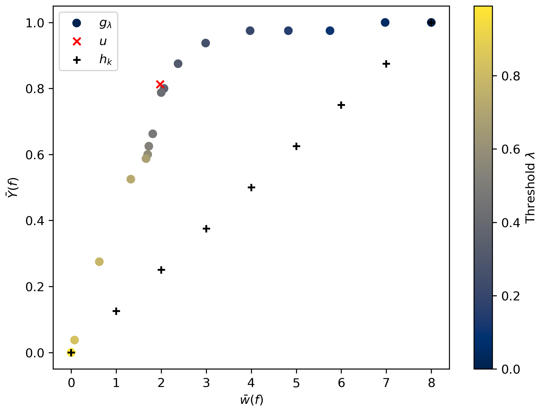
Figure 8 Results of scenario identification for different selection functions. Each point corresponds to one strategy f, and its coordinates correspond to the average number of scenarios retained $\stackrel{\mathrm{‾}}{w}\left(f\right)$ and the success rate $\stackrel{\mathrm{‾}}{Y}\left(f\right)$, computed over all 80 cases. The black-cross markers refer to the dummy strategies h_k, selecting a constant number of random scenarios. The dot markers refer to the strategies g_λ, retaining the scenarios with a cross-similarity over the threshold λ, with their color corresponding to the value of λ according to the color bar on the right. Finally, the red-cross marker refers to the strategy u, selecting the scenarios with the maximal cross-similarity. We can notice that both strategies g_λ and u are above the line of the random strategies h_k.

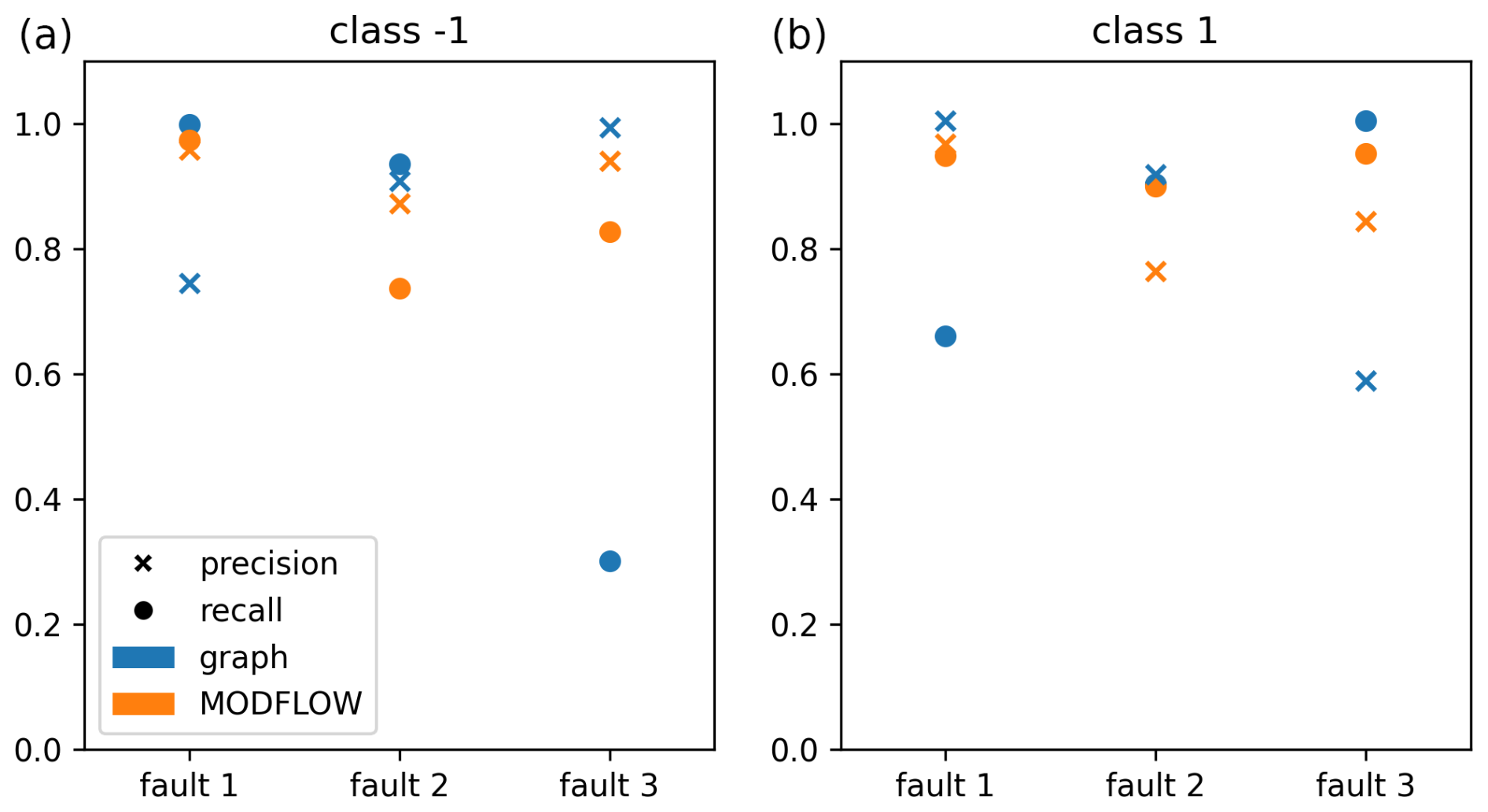
Figure 9 Precision and recall for the classification for each fault, each method, and each class. (a) Class −1 (barrier) and  (b) class 1 (path).

We can make the general observation that the results from the graph-based models are within the range of the results from the physics-based solver. Notably, for fault 2, the graph-based model even outperforms the physics-based one in predicting its behavior. This is because the graph method is highly sensitive to the presence or absence of paths with very high conductivity. Conversely, for fault 3 (the transverse fault), the results are significantly worse. This is because the Dijkstra paths are minimally influenced by the nature of fault 3 due to its geometry: whether it acts as a preferential pathway or as a barrier, it only adds a constant to the length of all of the paths.

4 Discussion

This study has confirmed and extended the findings of Rizzo and de Barros (2017) by successfully demonstrating the effectiveness of graph-based methods in approximating contaminant transport in 3D subsurface environments with faults. Using a graph modelization very similar to the one of Rizzo and de Barros (2017), but embedding a few improvements, we have shown that not only the shortest path but the whole distance map generated by Dijkstra's algorithm between the source and the model's outlet is rank correlated with the distribution of cumulative masses flowing through the outlet. The proposed metric, combining both the Jaccard index and Wasserstein distance and used to compare the graph-based distances with the cumulative mass, is effective in comparing binary images and exhibits fairly good spatial similarity between the two maps.

The proposed similarity metric tries to mitigate the drawbacks of each of its components. On the one hand, the Jaccard index penalizes the comparison of small areas as a single-pixel error might significantly impact the IoU ratio in that case, and it cannot discriminate between non-overlapping scenarios. On the other hand, the NWD penalizes cases where a dissimilar pixel is very far from the areas of similarity between two images. However, one can note that it is very sensitive to slight changes: a small shift both decreases the Wasserstein component of the similarity and decreases the Jaccard index.

In addition to the model presented in Sect. 2.1, we tested our method in the absence of faults by varying the multi-Gaussian field. The results are presented in Appendix A. We first verified that our results align with those of Rizzo and de Barros (2017). We also studied the uncertainty of the minimal distance point of the outlet and compared it with that of the maximum cumulative mass point. We demonstrated that the uncertainties were comparable and followed similar trends for different field parameters. However, the absence of very-high-conductivity paths (or very-low-conductivity barriers), which the graph approximates quite well, can explain the mitigated performance of a graph-based approach in a multi-Gaussian setting. So, the use of the proposed approach is particularly interesting in testing scenarios displaying strong hydraulic conductivity contrasts or very different pathways.

These results suggest the potential use of graph-based methods as a proxy for groundwater flow simulation, particularly when traditional methods are too costly to implement and when the sought-after information is less about the contaminant concentration values and more about its location on a control plane. This is relevant for scenario selection, which can be achieved by comparing the locations of contaminants at the outlet. Our experiment described in Sect. 2.5 allowed us to assess the use of a graph-based method in fault scenario selection. By comparing the similarity between the cumulative mass result of a reference scenario and the graph simulations, we can either reject a significant number of scenarios to reduce uncertainty or calculate a fault-by-fault probability of increasing or decreasing the conductivity. For two of the three faults studied, our results are close to those obtained with MODFLOW 6.

However, several questions and challenges related to the use of graph-based methods remain unresolved after this study. It is still necessary to explore the impact of the chosen observation time for the physical data, as well as the possibility of 3D visualization of the shortest paths, and to test other graph algorithms for approximating groundwater flow. Additionally, the difficulty in determining a thresholding method for the distance seems to compromise the possibility of completely replacing physics-based methods. All of these questions are detailed in the following paragraphs.

An aspect to consider is the attention given to the observation time. As mentioned in Sect. 2.3, we chose to perform all our measurements at the first time of arrival (FTA). While we use a percentage approach to determine the FTA, an alternative could be to use a deconvolution approach (Luo and Cirpka, 2008), potentially with greater computing expenses. Then, with our dataset, we can calculate the time at which the distribution of cumulative mass is closest to the distribution of distances. However, it would be necessary to study the quality of the approximation at other observation times as well.

Additionally, it would be interesting to test the scalability of the approach (e.g., by increasing the regular grid resolution or simplifying the graph representation) or other graph algorithms to approximate groundwater flow to potentially increase the computing efficiency of the approach. In particular, the minimum-cost flow problem (Ahuja et al., 1993) could be useful if it can be properly defined in this context. Specifically, it would be necessary to find a geological value to associate with the notion of capacity, knowing that hydraulic resistance can be used to represent the cost.

With this graph-based method, we can hope for a true 3D visualization of the plume shape rather than just the distance distribution at the outlet. We have conducted some preliminary tests in this direction. The initial idea was to recalculate the distances between the source and each orthogonal section of the graph using Dijkstra's algorithm rather than just the final section. However, this method was unsuccessful due to the lack of consistency in the distance distribution between different sections. A more successful idea was to calculate the number of paths passing through each node in the 3D mesh to identify the most visited nodes. Preliminary figures are presented in Appendix C. A more quantitative study, such as comparing results with streamline-based approaches, would be necessary.

Finally, there are two paths open to make the graph-based method fully independent from the physics-based results. The first would be to find a thresholding method to distinguish the pixels of interest solely based on their distance. We attempted this in Appendix B, but our results were mixed. The second, more ambitious method would be to find a function Φ that transforms the distance distribution I_d into an estimate of the cumulative mass ${\widehat{\mathbf{I}}}_{\text{mf}}=\mathrm{\Phi }\left({\mathbf{I}}_{\mathrm{d}}\right)$. Machine learning approaches could be considered for this. Developing a truly independent method could significantly reduce computation time as graph generation and Dijkstra's calculation are 10 times less costly than a physics-based simulation.

The investigation of the use of graph structures as proxies for geological processes extends beyond the hydrogeological application proposed here. While our work could have more general applications to flow and transport in porous media, it has not been tested yet and could be investigated in future research. Regarding other fields of application, Montsion et al. (2024) used Dijkstra distances as proxies for the non-Euclidean distance in 2D between geological feature by assigning weights to edges based on estimated flow properties, and these distances were, in turn, used as part of a mineral prospectivity analysis. In the context of building 3D geological models, graph neural networks are being used as a framework for understanding relationships between observations (Hillier et al., 2021, 2023). In both cases, the possibilities for constraining the modeling results with knowledge graphs that share similar architectures (Enkhsaikhan et al., 2021) provide the potential for mapping specific local knowledge onto larger poorly understood regions.

5 Conclusions

GraphFlow allows for the calculation of Dijkstra paths to generate a distance map for the last layer of the model. We have demonstrated, by developing an appropriate similarity measure, that, for a synthetic case involving a fault zone, these distance maps are highly rank correlated (average Spearman coefficient of 0.9) with the distribution of cumulative masses at the first time of arrival (FTA). Moreover, the spatial similarity of the pixels of interest is high (0.62 on average for our similarity measure).

This result has enabled us to use this model for scenario selection. For eight different fault scenarios, comparing their distance maps significantly reduces uncertainty by selecting a few plausible scenarios with confidence.

Several challenges remain in finding other applications for this method. The main challenge is in making the model independent of physics-based results: specifically, finding a threshold based solely on distance to distinguish between pixels of interest and pixels with negligible cumulative mass.

Appendix A: Validation of the graph-based approximation method in a heterogeneous environment without faults

We also tested our graph-based approximation method in a heterogeneous environment without faults. We used the exact same parameters, but instead of testing variability according to fault behavior, we simulated 50 multi-Gaussian realizations for each geological unit, resulting in 50 different scenarios. There is only one source position with coordinates of x_s=1050 m, y_s=2550 m, and z_s=512.5 m.

As in the main body of the paper, the distribution of similarity was calculated, with the mean and median being 0.37 and 0.38, respectively. These results, shown in Fig. A1, are significantly lower but still acceptable (above the qualitative threshold of 0.3). This can be explained by the absence of very-high-conductivity paths (or very-low-conductivity barriers), which the graph approximates quite well.

For these simulations, we also found it interesting to study the sensitivity of the groundwater flow simulation results to the parameters of the multi-Gaussian hydraulic conductivity field. This has already been tested in numerous papers for PDE-based methods only.

Cao et al. (2018) show that the characteristic size of the plume for a 2D simulation and its variance (its uncertainty) increase when the field variance σ increases and also when the correlation length λ increases. Srzic et al. (2013) also demonstrate that, as the heterogeneity of the field increases, the uncertainty about the center of the plume increases as well. We would like to see if the results from the shortest-path method exhibit similar behavior in response to parameter changes.

Starting from reference values for the standard deviation σ₀ and the correlation length λ₀, we successively apply a factor to vary both parameters. The variable we will focus on is the standard deviation of the position of the point of maximum cumulative mass at the FTA (respectively, the point of minimal distance). For each standard deviation σ and correlation length λ, we generated 50 realizations of the MG field and calculated the standard deviation of the coordinates of the point of maximum cumulative mass at the FTA (respectively, the point of minimal distance). This represents the uncertainty of the result for the fixed parameters of standard deviation σ and correlation length λ considering the fact that the exact structure of the conductivity field is often unknown. By decomposing the results on the y and z axes, we can visualize the results in Fig. A2. We can observe that, in all cases, the results from Dijkstra's algorithm follow the trends of the MODFLOW 6 results. Moreover, these trends are consistent with previously observed results in the literature: as the correlation length and standard deviation increase, the uncertainty also increases. We can also notice the standard deviations from Dijkstra's algorithm are either equal to or significantly greater than those from MODFLOW 6. This means that the uncertainty related to the structure of the conductivity field is not underestimated by Dijkstra's method.

Figure A1 Histogram of the similarity index values over all 50 scenarios.

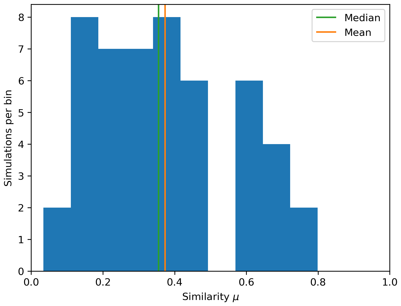
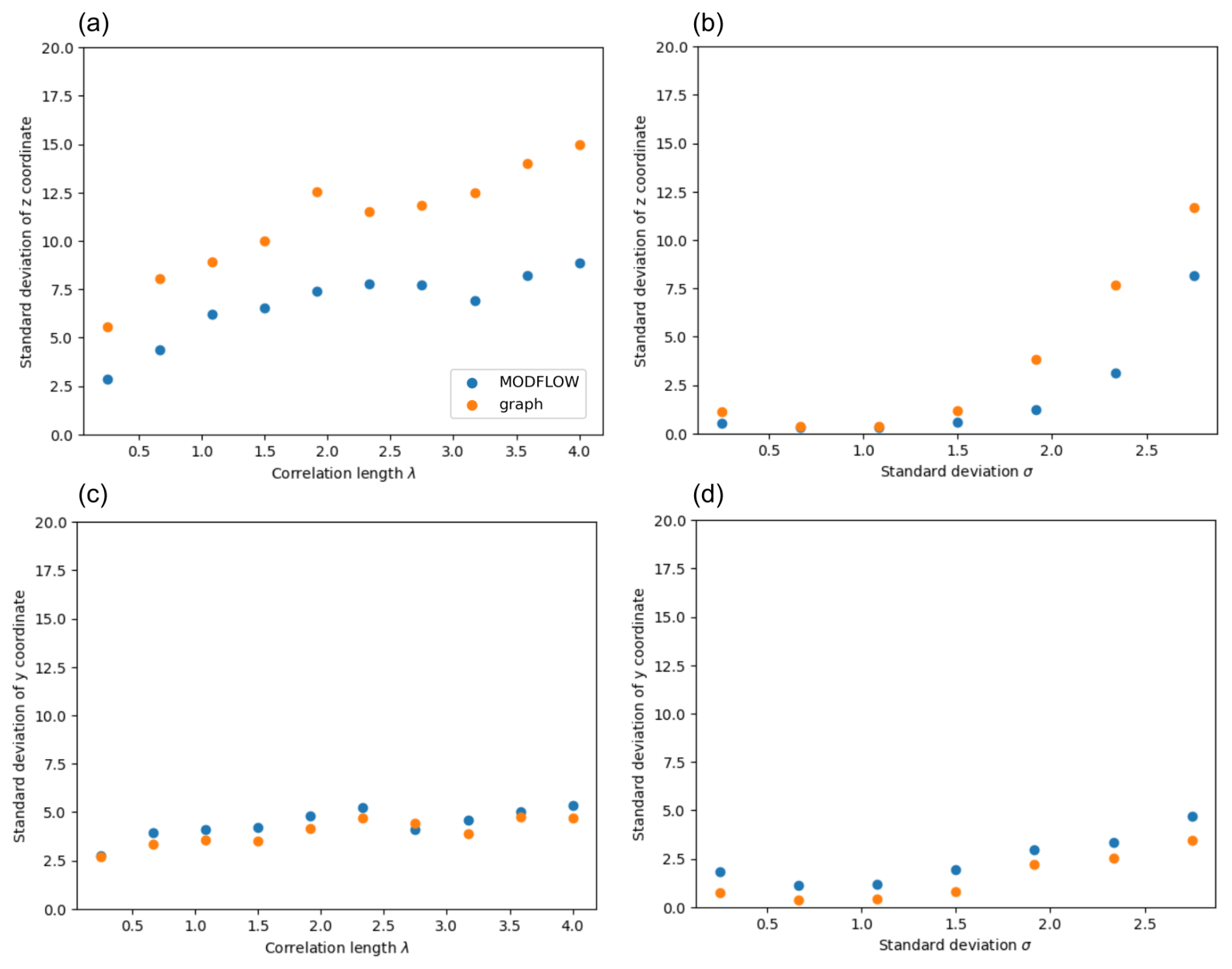
Figure A2 Standard deviation of point of maximum cumulative mass coordinates (respectively, point of shortest graph distance coordinates) for simulations with MODFLOW 6 in blue (respectively, with graph method in orange) as a function of the correlation length of the conductivity field.

Appendix B: Thresholding methods for identifying significant points based on distance

In Sect. 3, we observed the effectiveness of similarity: for a given number n of pixels (corresponding to the number of pixels where the cumulative mass at FTA is significant), we compared the set of n pixels with the highest cumulative mass at FTA X_m with the set of n pixels with the smallest distance X_d. However, even with this knowledge, without physics-based data I_m, there is no straightforward way to determine which points of I_d should be retained as locations where the contaminant is present in significant quantities based solely on the ranking of points according to their distance. For instance, we cannot predict whether the cumulative mass is uniform throughout the entire last layer or highly localized. Therefore, we aim to automatically determine, using the distribution of distances, a threshold to distinguish between significant and other points, returning an estimation of the area ${\widehat{\mathbf{I}}}_{\text{dk}}$ where the contaminant is significant. The Otsu algorithm does not work well directly on the distance array I_d because the distribution is not suitable for it. By examining the distributions of several scenarios (see Fig. B1a and b), we observe the presence of a peak, typically close to the minimum distance. Empirically, a correct threshold value consistently lies before this peak.

An attempt we made was to apply an Otsu thresholding to the signal before this peak. It is even possible to use multi-class Otsu thresholding to estimate different cumulative mass zones. The results are mixed, and some examples are shown in Fig. B1c and d. Often, our auto-thresholding attempt overestimates the area of interest.

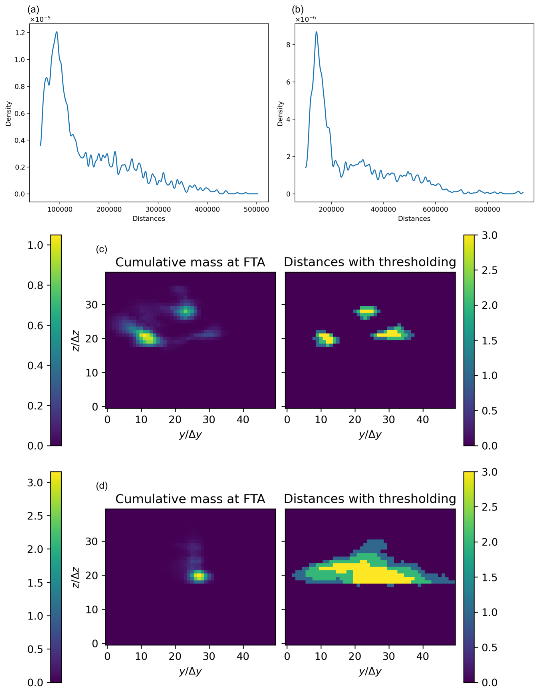
Figure B1 (a, b) Densities of the distance for two different simulations. The densities have been computed with a Gaussian kernel. The presence of a peak close to the shortest distance is to be noticed. (c, d) Two different cases and their corresponding estimated thresholding based on the distances. In both cases, the similarity is already quite good (>0.5). The color bars on the right refer to the discrete classes after the Otsu thresholding; this is not meant to approximate the cumulative mass values. The axes are expressed in discretization units.

Appendix C: A 3D visualization of Dijkstra pathways

For each vertex, we aim to count the number of Dijkstra paths that pass through these nodes. Using the notations from Sect. 2.2.1 and calling $({\mathit{\pi }}_{\mathrm{1}},\mathrm{\dots },{\mathit{\pi }}_{\mathrm{2000}})$ the set of oriented paths calculated by Dijkstra's algorithm between the source and the 2000 nodes of the model outlet face, we define the number of paths passing through a vertex v∈V as n^*(v):

$$\begin{array}{}\text{(C1)}& n^{*}\left(v\right)=\sum _{i\in \mathit{\{}\mathrm{1},\mathrm{\dots },n\mathit{\}}}{\mathbb{1}}_{v\in {\mathit{\pi }}_i},\end{array}$$

where ${\mathbb{1}}_{\mathit{\{}v\in {\mathit{\pi }}_i\mathit{\}}}$ is an indicator function that equals 1 if the vertex v belongs to the path π_i and that equals 0 otherwise.

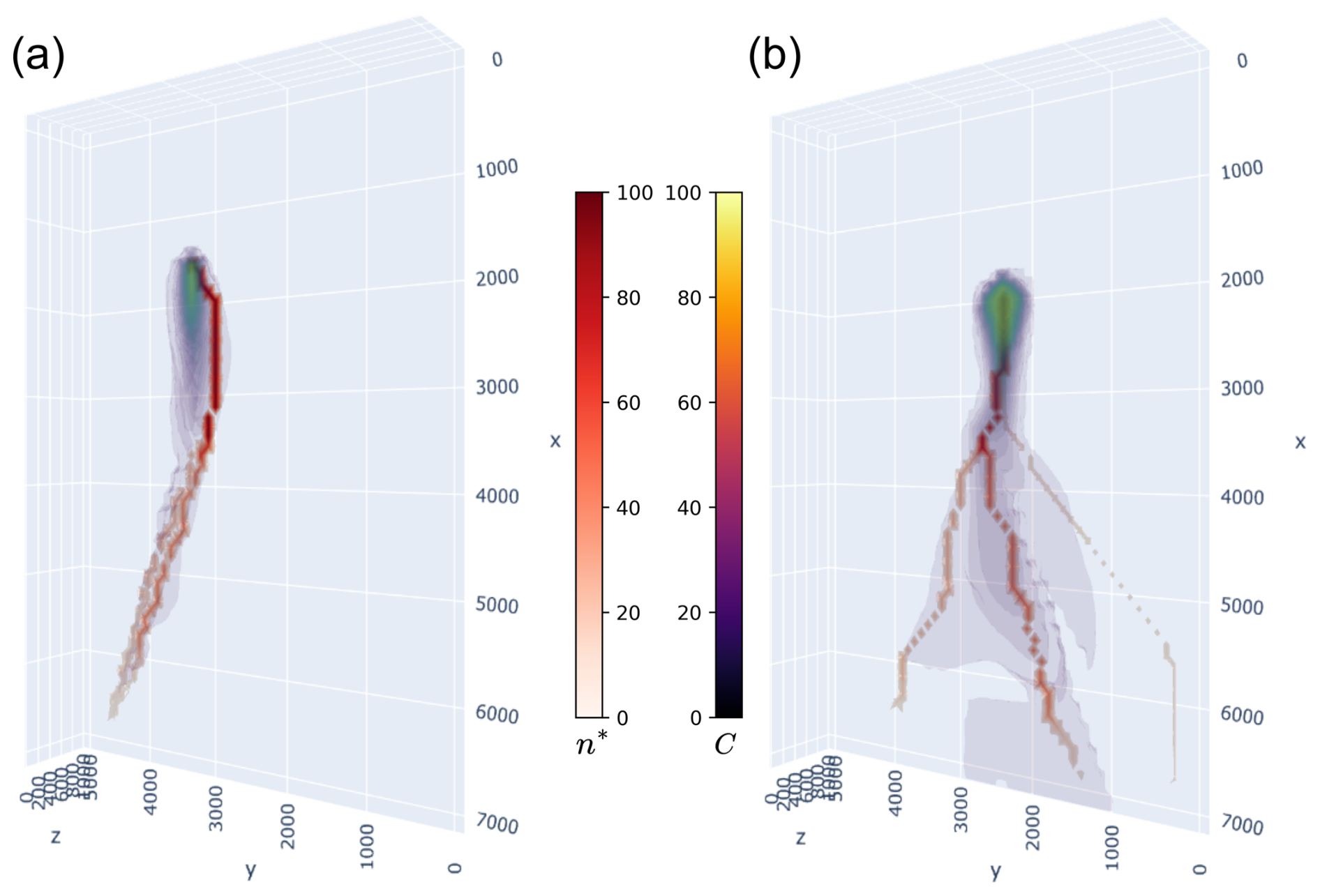
Figure C1 Visualization for two scenarios of the most visited nodes n^* and the concentration C at FTA.

In practice, if we consider all of the paths between the source and the last layer, we end up with nodes with a high n^* value, but these do not accurately correspond to the actual flow paths of the contaminant. This occurs because arrival points that are very far away or even at an infinite distance (in the sense of Dijkstra) from the source are counted, meaning the contaminant has no chance of reaching them. Thus, we realized that restricting the number of nodes to m by selecting only the m closest nodes (in the sense of Dijkstra) in relation to the source yielded better results. For the examples, we arbitrarily chose m=200, but this parameter warrants further exploration. Some examples of this method are shown in Fig. C1.