Enhanced land subsidence interpolation through a hybrid deep convolutional neural network and InSAR time series

Land subsidence, whether gradual or sudden, poses a significant global threat to infrastructure and the environment. This study introduces a hybrid approach that combines deep convolutional neural networks (CNNs) with persistent scatterer interferometric synthetic aperture radar (PSInSAR) to estimate land subsidence in areas where PSInSAR data are unreliable or sparse. The proposed method trains a deep CNN using subsidence driving forces and PSInSAR data to learn spatial patterns and predict subsidence values. Our evaluation demonstrates that the CNN effectively mitigates discontinuities in PSInSAR results, producing a continuous and reliable subsidence surface. The model's performance was assessed using training, validation, and testing datasets, achieving root mean square errors (RMSEs) of 3.99, 8.47, and 9 mm, respectively. In contrast, traditional interpolation methods such as kriging, inverse distance weighting (IDW), and radial basis function (RBF) interpolation yielded RMSE values of 61.60, 66.21, and 61.76 mm, respectively, on the test dataset. Additionally, the coefficients of determination (R²) for CNN, kriging, IDW, and RBF were 0.98, −0.06, −0.22, and −0.06, respectively. The deep CNN model demonstrated an 85 % improvement in subsidence prediction accuracy compared to conventional interpolation methods, highlighting its potential for accurate and continuous land subsidence estimation.

1 Introduction

The gradual decrease in the height of Earth's surface, which is accompanied by slight horizontal displacements, is called subsidence. Due to the gradual nature of land subsidence, this phenomenon is also called “silent earthquake”. Its harmful effects appear over a long period of time and carry significant risks. However, land subsidence is a global threat to urban areas around the world (Sun et al., 2023). This issue is an important global concern and is not limited to one region. Iran is facing an increasing challenge, especially in this field. Human activities, such as mining and excessive underground water extraction, contribute to this problem. To address it, effective groundwater management to prevent unauthorized water extraction would help. However, land subsidence is not only caused by human actions; natural factors also play an important role. These include water table fluctuations, soil characteristics, bedrock depth, terrain features such as elevation and aspect, vegetation cover, and the prevailing climate. All of these factors together create a complex landscape of land subsidence occurrences.

Precise levelling and GNSS observations offer high precision in measuring subsidence, but their use in investigating subsidence over a wide area is limited due to their reliance on measuring sparse stations. These methods require multiple measurements at different locations, making it difficult to monitor subsidence over large areas (Fialko et al., 2005; Hu et al., 2012). However, interferometric synthetic aperture radar (InSAR) has a high spatial resolution and has emerged as a cost-effective technique for monitoring subsidence on a large scale (Amighpey and Arabi, 2016; Biswas et al., 2018; Chang et al., 2010; Gonnuru and Kumar, 2018; Khorrami et al., 2019; Rucci et al., 2012; Tamburini et al., 2010; Tomás et al., 2011). InSAR uses radar waves to carefully monitor changes in Earth's crust surface over time. Methods that analyse radar images over time, known as time series analysis, make them very effective for monitoring subsidence, which usually occurs gradually over time. Persistent scatterer interferometric synthetic aperture radar (PSInSAR) is particularly valuable for monitoring urban land subsidence. This is because there are many high-density persistent scatterer (PS) points, mainly associated with buildings and anthropogenic structures. This abundance significantly improves the quality of the data within interferograms (Gao et al., 2019). Although these advantages are significant, dealing with the sparse and uneven distribution of PS points in both the spatial and temporal dimensions is a significant computational challenge. The PSInSAR approach generates discontinuous results, as it calculates subsidence exclusively at PS points. Consequently, it becomes imperative to employ intelligent interpolation instead of mathematical or stochastic methods between these data points to fill out these gaps (Naghibi et al., 2022).

Subsidence is a complex physical phenomenon influenced by a multitude of factors, such as changes in groundwater levels, soil type, bedrock depth, slope, elevation, and aspect. To obtain the subsidence in the whole area, interpolation methods between PS points and artificial intelligence (AI) methods (where AI is trained using features affecting subsidence) can be used to obtain subsidence information for the entire area. Classical interpolation methods (e.g. kriging, inverse distance weighting (IDW), radial basis function (RBF), Mehrabi and Voosoghi, 2018; recursive moving least squares (RMLS), Mehrabi and Voosoghi, 2015) do not consider the physics of the issue, making their results less reliable. So it is very important to apply methods that take into account the real characteristics of the phenomenon, especially when monitoring the subsidence. Recently, machine learning methods, specifically deep convolutional neural networks (CNNs), have shown encouraging results in various applications. In the larger context of land subsidence prediction models, we find two main categories: (1) physical process models simulate subsidence by incorporating factors such as geotechnical mechanics, soil properties, and water dynamics. They are frequently used in large-scale projects but require a substantial amount of prior knowledge and data (Nie et al., 2015); and (2) mathematical or statistical models that predict subsidence based on historical elevation data and past trends (Zhu et al., 2010).

Several studies have investigated various forecasting models, methodologies, and influencing factors to improve the understanding of this field. Neural networks have emerged as powerful prediction tools and have been used in the field of subsidence prediction using its driving forces (Azarakhsh et al., 2022; Ku and Liu, 2023; Zhu et al., 2010). Lee et al. (2023) employed data from an urban area in South Korea to develop a machine-learning-based model for predicting land subsidence risk. Their methodology incorporated historical land subsidence data along with attribute information pertaining to underground utility lines in the specified region. The research team utilized machine learning algorithms such as random forest (RF), extreme gradient boosting (XGBoost), and light gradient boosting machine (LightGBM) for the analysis and prediction of land subsidence risks (Lee et al., 2023). Sadeghi et al. (2023) combined full consistency decision making (FUCOM) and GIS methodologies to assess Iran's vulnerability to land subsidence. Their approach resulted in the development of a hierarchical FUCOM-GIS framework, which highlighted critical factors such as water stress, groundwater depletion, soil type, geological timescale, and rainfall amount as the main drivers of land subsidence. Researchers commonly validate their results by comparing them with InSAR analyses, identifying areas exhibiting notable subsidence. Furthermore, the research assessed the risks to power transmission lines and substations, revealing structural issues such as pier sinking, electric insulator deviation, and cracking (Sadeghi et al., 2023). In another study focused on Dechen County, China, Wang et al. (2023) employed backpropagation neural network (BPNN) and RF algorithms in conjunction with various monitoring data sources, GIS, and small baseline subset (SBA) technology to predict trends in land subsidence. Their findings underscored Sugianto as the most severely affected area, with an annual average subsidence rate of −40.71 mm yr⁻¹. The study highlighted that changes in both deep and shallow groundwater levels were the primary drivers of land subsidence in this region. Notably, the BPNN model demonstrated higher prediction accuracy compared to the RF model, especially when considering changes in groundwater levels (Wang et al., 2023). Furthermore, Zhou et al. (2020) demonstrated that the integration of the GM (1,3) model with neural networks and ground-related variables shows great potential for achieving highly accurate subsidence predictions. The proposed approach is capable of replacing traditional precise levelling methods in long-term subsidence forecasting, offering valuable insights for urban disaster prevention (Zhou et al., 2020).

Deng et al. (2017) conducted research on the integration of PSInSAR with grey system theory for monitoring and predicting land subsidence, as demonstrated in the Beijing plain (Deng et al., 2017). Precision mapping of complete subsidence basins faces challenges, especially when dealing with image pairs with limited temporal separation. Rapid deformations and vegetative changes in such scenarios introduce complexity. Strategies, such as combining differential interferometric synthetic aperture radar (DInSAR) with the probability integral model (PIM), have been introduced to effectively delineate subsidence basins resulting from mining activities (Fan et al., 2015).

The remarkable effectiveness of the RF model in mapping the susceptibility of land subsidence deserves attention. This approach demonstrates exceptional capabilities in identifying key factors that contribute to subsidence occurrences, such as the proximity to faults, elevation, slope angle, land use patterns, and water table levels. These factors play a crucial role in influencing the likelihood of subsidence events (Mohammady et al., 2019). In addition, the integration of fuzzy logic techniques and neural networks has been used to predict subsidence (Ghorbanzadeh et al., 2020).

Land subsidence is a significant geological risk, and predicting and investigating this phenomenon is vital. Traditional monitoring and forecasting methods have limitations and require more advanced approaches. Kumar et al. (2022) utilized recurrent neural networks (RNNs), specifically vanilla and stacked long short-term memory (LSTM) models, to forecast land subsidence in the Jharia Coalfield, Dhanbad, India. Using data from 14 locations collected through the modified PSInSAR technique, the study shows that these models can effectively predict deformation rates, identifying critical subsidence levels at Nai-dunia basti, Digwadih, and Godhar. This research underscores the potential of integrating advanced monitoring techniques with sophisticated predictive models to better anticipate and mitigate land subsidence impacts (Kumar et al., 2022).

The integration of InSAR processing with deep-learning methods in modelling and predicting land subsidence has shown significant promise. This approach demonstrates substantial capabilities in identifying and predicting subsidence in regions around Lake Urmia by leveraging Sentinel-1 data and SBA InSAR methods. Key factors such as rainfall, groundwater levels, and lake area variations, measured using TRMM, GRACE, and MODIS satellite data, were critical in understanding subsidence dynamics. Moreover, the application of machine learning models, including multi-layer perceptron, CNN, and LSTM networks, has been instrumental in improving prediction accuracy. The ensemble model combining these networks outperformed individual models, achieving enhanced prediction reliability (Radman et al., 2021).

Predicting deformation is essential for early detection of abnormal conditions and timely intervention. A recent study introduced a deep convolutional neural network (DCNN) approach to forecasting time series deformation using InSAR data. The research, conducted at Hong Kong International Airport, demonstrated that the DCNN could effectively predict both linear land settlement and nonlinear thermal expansion of structures with high accuracy. The study's findings highlight the DCNN's potential to enhance early warning systems by providing precise short-term deformation predictions, thus enabling better risk management and mitigation strategies (Ma et al., 2020).

In this study we used a CNN model trained over the area where subsidence is available through PSInSAR. Then this model is used over other areas where subsidence cannot be obtained from PSInSAR processing. The proposed method follows three main steps: calculation of subsidence in PS points by PSInSAR method, calculation of subsidence driving forces, and training CNN.

2 Methodology

2.1 PSInSAR

PSInSAR is a remote sensing technique that utilizes SAR images to monitor surface deformation over time. It relies on identifying PS points, which are stable points on Earth's surface reflecting radar signals consistently. PSInSAR combines multiple interferograms created by comparing synthetic aperture radar (SAR) images of the same area taken at different times. By analysing phase differences between radar signals in these interferograms, it detects changes in Earth's surface over time. PSInSAR has significant advantages over DInSAR, as it effectively eliminates topographic errors and atmospheric noise, and it addresses temporal and spatial correlation issues between radar images (Ferretti et al., 2001; Gonnuru and Kumar, 2018; Wasowski and Bovenga, 2014). PSInSAR, a form of differential interferometry, involves analysing a collection of at least 15 SAR images captured at different times, all covering the same area (Crosetto et al., 2016). PSInSAR finds diverse applications, including monitoring subsidence in urban areas (Ferretti et al., 2000; Luo et al., 2013) and tracking natural hazards such as landslides, earthquakes, and volcanic activity (Peltier et al., 2010). However, one drawback of PSInSAR is the lack of continuity between PS points, as they depend on the land use of the area. These PS points are more abundant in areas with buildings, dams, oil wells, pipelines, electric fences, roads, rocks, and bridges (Din et al., 2015), but they are relatively scarce in vegetated areas. Consequently, PSInSAR performs best in urban areas and regions with rocky terrain (Oštir and Komac, 2007).

In this article, the amplitude dispersion index is used to select the PS points, Eq. (1). The usual threshold of the amplitude dispersion index is limited between 0.2 and 0.4 (Conway, 2016).

$$\begin{array}{}\text{(1)}& D_{\mathrm{A}}={\mathit{\sigma }}_{\mathrm{A}}/{\mathit{\mu }}_{\mathrm{A}},\end{array}$$

where μ_A and σ_A are the standard deviation and mean values of the radiometrically corrected amplitude of pixels. In PSInSAR the amplitude data from SAR images is carefully examined to identify specific PS points while excluding those affected by space–time decoherence and atmospheric delay (Li et al., 2004).

2.2 Deep CNNs

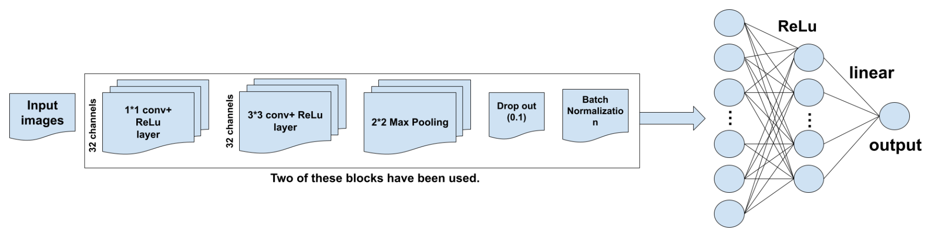
CNNs are deep-learning algorithms widely employed for various image-related tasks such as image recognition, classification, and regression. They learn and extract essential features from raw images by processing them through multiple layers of filters, known as “convolutions”. This multi-layer processing progressively extracts more abstract features. These filters are trained using backpropagation, a technique that adjusts filter weights based on the difference between the predicted and actual outputs. In addition to convolutional layers, CNN typically includes pooling layers to downsample the convolutional output and fully connected layers to use the extracted features for image classification. CNN has gained popularity, particularly after the success of AlexNet in the ImageNet challenge in 2012, and has since become the dominant approach for image recognition tasks.

CNN is used in various fields, including medical imagery (Lee et al., 2017), classification (LeCun and Bengio, 1998), segmentation (Nair and Hinton, 2010; Van Do et al., 2024), image reconstruction (Christ et al., 2016; Elboushaki et al., 2020; Lakhani and Sundaram, 2017), and natural language processing (Kim et al., 2018). While CNN are often associated with categorical tasks, they are also highly effective in regression tasks, where the goal is to predict continuous output variables instead of discrete labels. In CNN regression, the network typically has a single output neuron in the final layer that generates a continuous value instead of a probability distribution for classification. It is important to note that CNN requires a lot of input data, especially for image processing. As the network's depth increases, so does its complexity, resulting in a larger number of weight parameters, which can sometimes create challenges during training (Liu et al., 2018). CNN introduced the concept of local connections between layers with typical components including convolution, activation, and pooling layers (Chen et al., 2018). The convolutional layer learns image features from small sections of input data through mathematical operations involving the input image matrix and a filter or kernel. The activation layer introduces nonlinearity into the network, commonly using the rectified linear unit (ReLU) function.

CNN regression is a valuable approach for predicting continuous output variables and has found applications in various fields including geology and civil engineering. CNN regression can also be used to predict subsidence. By training a CNN model with input–output pairs, where inputs are subsidence driving forces and outputs represent subsidence values, researchers can predict subsidence at single-pixel levels and provide valuable insights.

To predict land subsidence, we trained a CNN regression model with the architecture shown in Fig. 1. The CNN has 31 layers, including three 1×1 convolutional layers, three 3×3 convolutional layers followed by three 2×2 max-pooling layers, batch normalization layers, drop out layers with a rate of 0.1, and two fully connected layers with 1024 rectified linear unit (ReLU) activation neurons, two fully connected layers with 512 ReLU activation neurons, and a fully connected layer with 256 ReLU activation neurons. The input dimensions are $\mathrm{30}\times \mathrm{30}\times \mathrm{9}$, where 30×30 patches separated from the neighbourhood of each scattered point and 9 features are used as network input.

Figure 1 Illustration of CNN architecture.

2.3 Hyperparameter tuning process

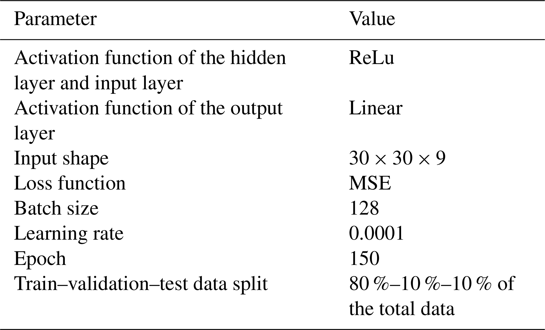
After creating the model architecture, model inputs were normalized to a range of [0,1] to ensure consistent input scaling, which is crucial for the stable performance of the neural network. Then we tuned the hyperparameters of the CNN regression model, including the loss function, optimizer, batch size, learning rate, activation function, and number of epochs. The best model was saved based on its performance metrics. The optimal parameters for the model are given in Table 1, and the rationale for each hyperparameter is explained in detail below.

• Activation function. We used the ReLU function in the hidden layers due to its effectiveness in mitigating the vanishing gradient problem and promoting sparse activations. For the output layer, a linear activation function was employed to ensure the model could predict a continuous range of values.

• Loss function. We considered both the mean squared error (MSE) and the mean absolute error (MAE) as potential loss functions. The MSE penalizes larger errors more heavily than the MAE, making it suitable for scenarios where outliers significantly impact the model's performance. Given the MSE's properties and its ability to improve the model's performance by reducing fluctuations and speeding up convergence, we selected MSE as our loss function. The MSE is calculated as follows:

  $$\begin{array}{}\text{(2)}& \text{MSE}={\displaystyle \frac{\mathrm{1}}{N}}{\sum }_i^N(Y_i-{\widehat{Y}}_i{)}^{\mathrm{2}},\end{array}$$

  where Y_i represents the actual values, ${\widehat{Y}}_i$ represents the predicted values, and N is the number of observations.

• Batch size. We experimented with batch sizes of 64 and 128. A larger batch size of 128 was chosen as it provided a good balance between training speed and model performance, allowing more stable gradient estimates.

• Learning rate. The initial learning rate was set to 0.001, but we found that a smaller learning rate of 0.0001 led to more gradual and stable convergence, reducing the risk of overshooting the optimal solution.

• Optimizer. The Adam optimizer was selected for its adaptive learning rate capabilities and efficiency in handling sparse gradients. It combines the advantages of both the AdaGrad (Adaptive Gradient Algorithm) and RMSProp (root mean square propagation) algorithms, making it suitable for our regression task.

• Number of epochs. We initially set the number of epochs to 100 but extended this to 150 epochs to ensure the model had sufficient time to learn the underlying patterns in the data without overfitting.

• Dividing the data. We initially allocated 15 % of the total data to the test data, 15 % to the validation data, and 70 % to the training data. However, we observed high-cost function fluctuations in the training and validation data. To mitigate this issue, we adjusted the data split to 80 % for training and 10 % each for testing and validation, which helped reduce the fluctuations

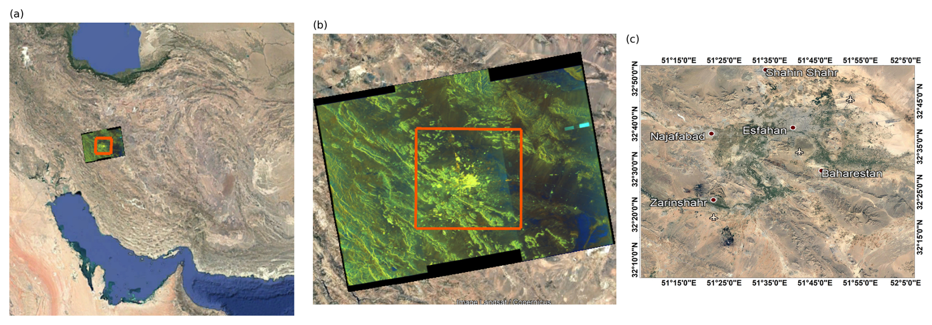
Figure 2 Geographic overview of the study area (© Google Earth).

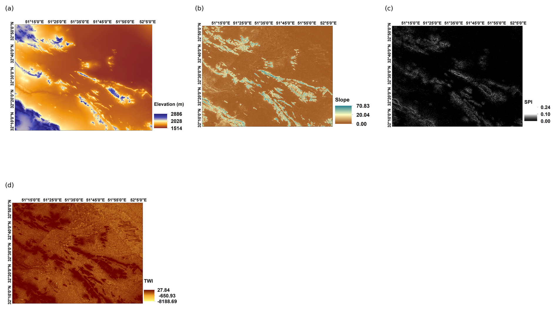
Figure 3 Subsidence driving forces – (a) elevation, (b) slope, (c) SPI, and (d) TWI.

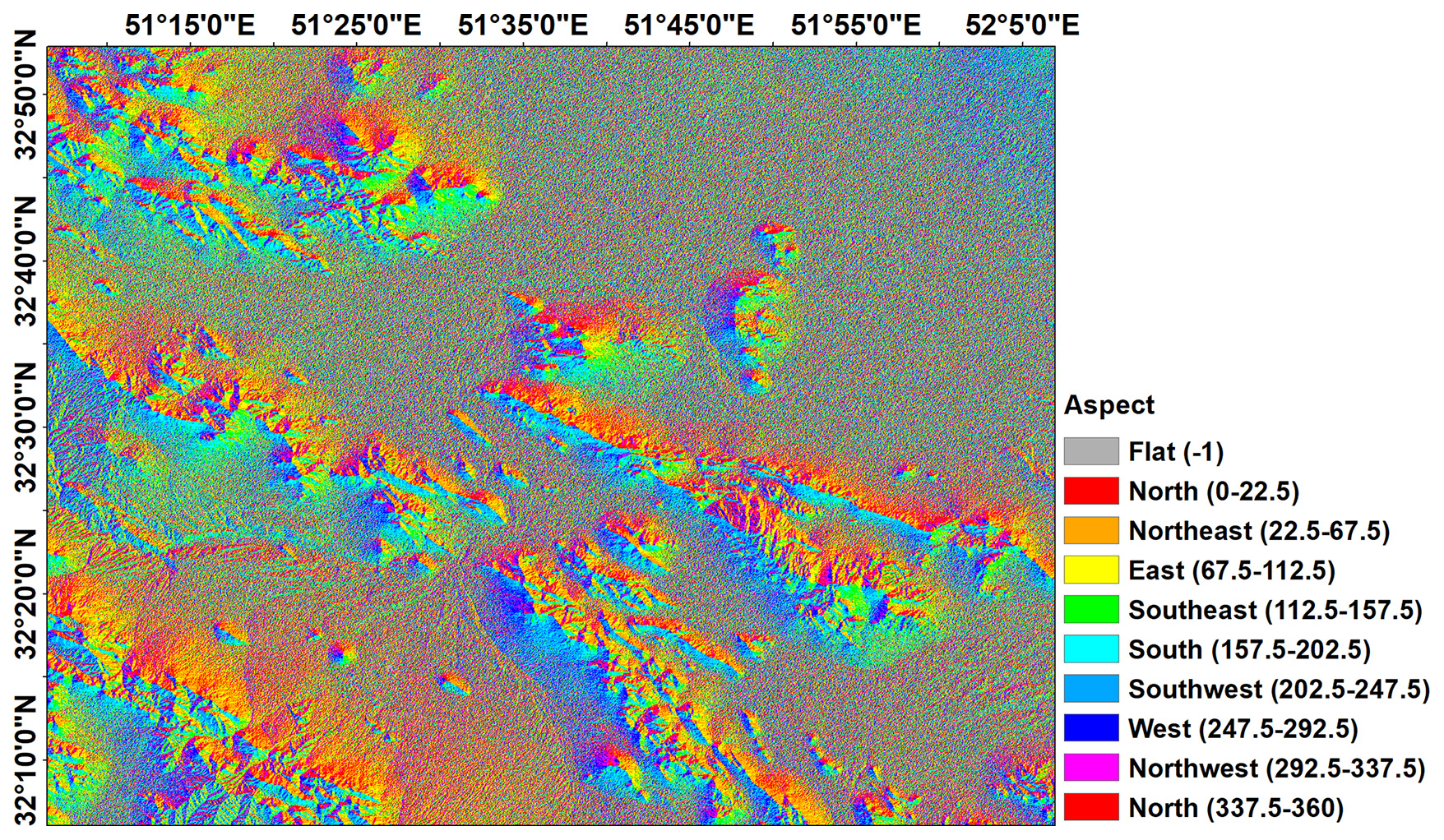
Figure 4 Subsidence driving force – aspect.

Table 1 Key parameters of the CNN.

2.4 Driving forces of subsidence

The selected driving factors for predicting subsidence – normalized difference vegetation index (NDVI), distance from wells, land use, water table map, altitude, slope, stream power index (SPI), topographic wetness index (TWI), and aspect – are well supported by extensive research and have been identified as significant predictors in previous studies (Abdollahi et al., 2019; Andaryani et al., 2019; Conway, 2016; Fan et al., 2015; Ghorbanzadeh et al., 2020; Mohammady et al., 2019; Shi et al., 2020; Wang et al., 2023; Yang et al., 2014; Zang et al., 2019; Zhao et al., 2021; Zhou et al., 2020). By incorporating these factors into the subsidence prediction model, this study ensures a comprehensive approach that reflects the complexity of subsidence phenomena.

1. NDVI is a crucial indicator of vegetation health and land cover changes. Changes in NDVI can reflect alterations in land use practices, such as urbanization or agricultural expansion, which are closely linked to subsidence. Healthy vegetation typically reduces the need for excessive groundwater extraction, while barren or urbanized areas might correlate with higher subsidence due to increased groundwater use.

2. The distance from groundwater extraction wells is a critical factor in subsidence studies. Areas closer to high-density exploitation wells often experience more severe subsidence due to the localized impact of extensive groundwater withdrawal.

3. Land use changes, including urbanization, agricultural expansion, and deforestation, influence subsidence rates. Urban areas often experience higher subsidence due to increased groundwater extraction for residential, industrial, and agricultural purposes.

4. Groundwater level changes, as depicted in water table maps, are directly linked to subsidence. Over-extraction of groundwater leads to a drop in the water table, causing the ground to compact and subsidence. Groundwater depletion is a primary contributor to subside, emphasizing the importance of preventing unauthorized withdrawals and effectively managing water resources.

5. Altitude influences subsidence through its effect on hydrological processes. Altitude affects the distribution and movement of groundwater. Higher altitudes typically receive more precipitation, which can infiltrate the ground and recharge aquifers. At lower altitudes, reduced precipitation and higher evaporation rates can lead to a lowering of the water table. When groundwater is extracted faster than it is replenished, it can result in subsidence. The amount of water in the soil, influenced by altitude through precipitation and drainage patterns, affects soil compaction. High altitude areas with abundant rainfall can lead to saturated soils which are less prone to subsidence. Conversely, in lower altitude areas with less precipitation, soils may dry out and compact more easily, contributing to subsidence.

6. Slope affects water runoff and infiltration rates. Steeper slopes may reduce infiltration, leading to less groundwater recharge and potentially higher subsidence rates in adjacent flat areas.

7. The SPI measures the power of water flow in depositing and causing soil erosion. As a result, this index can be an important input for subsidence prediction models. The equation used to calculate SPI is as follows (Pradhan et al., 2014):

   $$\begin{array}{}\text{(3)}& \text{SPI}=\mathit{\alpha }\cdot \tan \mathit{\beta }.\end{array}$$

   Here, α represents flow accumulation, and β represents the slope.

8. The TWI is a mathematical formula that quantifies the effect of local topography on the flow of surface water. It is a physically based index that can be used to determine flow direction and accumulation and has many practical applications in fields such as hydrology, agriculture, and geology. The TWI indicates areas of potential soil moisture accumulation. Areas with high TWI values are likely to have more groundwater recharge, which can mitigate subsidence.

   In rainfall runoff modelling, TWI can be used to predict the amount and timing of runoff in a specific area, while in soil moisture modelling it can be used to predict the spatial distribution of soil moisture. Overall, the TWI is a useful tool for understanding and predicting the movement of water across the landscape (Qin et al., 2011). Additionally, the TWI identifies areas that can be affected by flooding from rainfall events (Ballerine, 2017). The TWI equation is as follows (Moore et al., 1991):

   $$\begin{array}{}\text{(4)}& \text{TWI}=\ln (\mathit{\alpha }/\tan \mathit{\beta }),\end{array}$$

   where α is the upslope contributing area and β is the slope. The TWI is calculated using a digital elevation model (DEM) of the study areas.

9. Aspect affects solar radiation and, consequently, evaporation and soil moisture levels. Different aspects can lead to variations in vegetation cover and groundwater recharge, influencing subsidence. Additionally, the slope and aspect of an area can influence drainage patterns, erosion, and sediment production, all contributing to subsidence.

It is essential to recognize that examining one factor alone is not enough to predict subsidence. A linear relationship between groundwater level changes and subsidence may exist in certain regions, but this linear relationship does not exist in all regions. Each region has unique characteristics such as soil type, fault lines, and slope. Subsidence is a complex phenomenon that requires a comprehensive investigation that takes into account all relevant factors. Therefore, thorough analysis is necessary to obtain a comprehensive understanding of subsidence in a particular area (Azarm et al., 2023).

3 Study area and datasets

3.1 Study area

The studied area is in Isfahan Province and includes the cities of Isfahan, Mahyar, Khomeini Shahr, and Falavarjan. This region has a rich history of human habitation, a diverse cultural heritage, and a wide range of economic activities. Covering approximately 7000 square kilometres, this area displays various uses, including urban, agricultural, and industrial areas. Its climate is semi-arid, characterized by hot summers and cold winters. The primary sources of water in this area are the Zayandeh-Rud River and several underground aquifers that provide water for various uses such as agriculture, drinking water, and industrial needs (Neysiani et al., 2022) (Fig. 2). To effectively monitor and predict land subsidence in this study area, we used advanced techniques such as radar interferometry and CNN. Our goal was to provide an accurate and reliable estimate of land subsidence in the study area by integrating these techniques and considering complex subsidence driving forces.

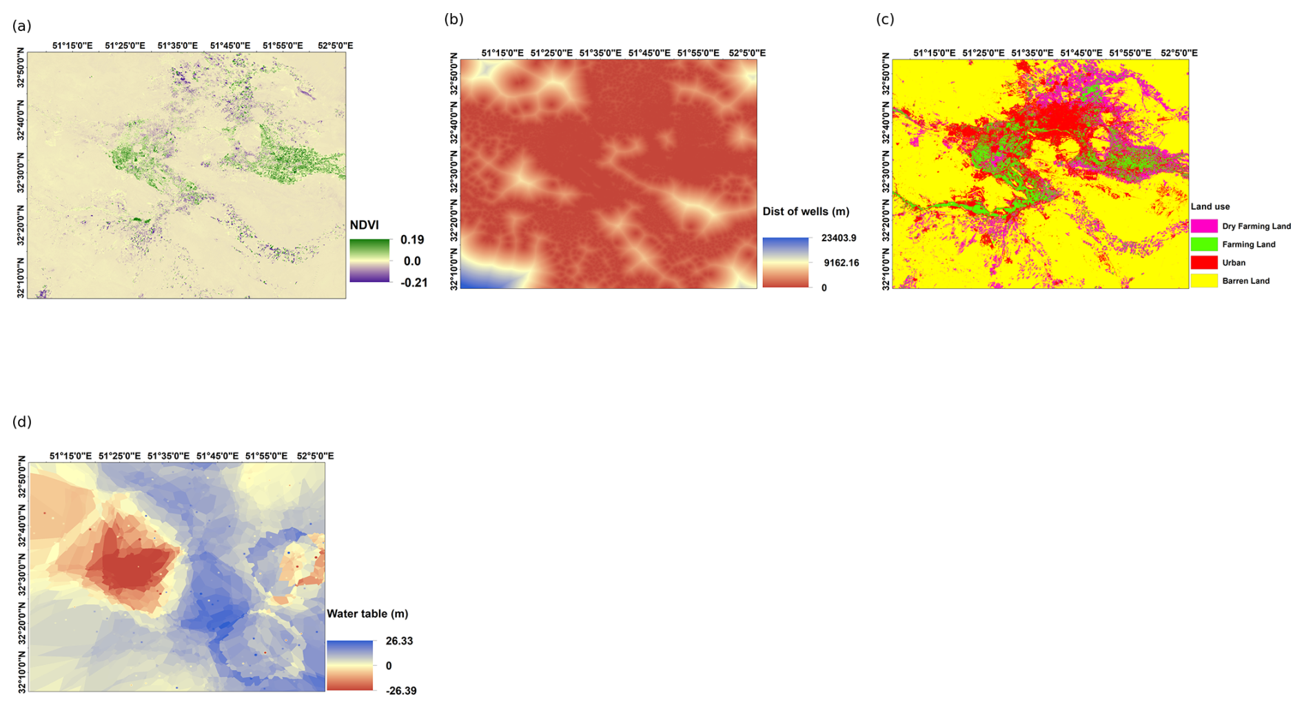
Figure 5 Driving forces of subsidence – (a) NDVI, (b) distance of wells, (c) land use, (d) water table map in 2014 to 2020.

3.2 Datasets

3.2.1 Sentinel-1A radar images

This study utilizes 73 radar images from the Sentinel-1A satellite to analyse subsidence trends in the study area over a 7 year period, from 2014 to 2020. The data were collected from the ascending track 28. The Sentinel-1A satellite, launched by the European Space Agency, operates in C-band and provides SAR imagery with a spatial resolution of 5 m by 20 m. The images were acquired at 6 d intervals, ensuring high temporal resolution for detecting ground movements. The interferometric wide swath mode was used, offering comprehensive coverage of the study area.

The PSInSAR technique was applied to the Sentinel-1A data using Sarproz software. This method is particularly effective in urban and semi-urban areas where permanent scatterers are abundant. The precise processing steps involved coregistration, interferogram generation, phase unwrapping, and geocoding to produce detailed subsidence maps (Ferretti et al., 2001).

3.2.2 DEM

The 30 m Shuttle Radar Topography Mission Digital Elevation Model (SRTM DEM) was employed to calculate various topographical and hydrological indices, including SPI, TWI, slope, and aspect. These indices were computed using ArcMap software, providing essential insights into the terrain characteristics influencing subsidence (Figs. 3 and 4).

3.2.3 Optical satellite images

Optical images from the Landsat 8 satellite, launched by NASA, were used to extract NDVI and land use information for the year 2020. The Landsat 8 images, with a spatial resolution of 30 m, were processed using Envi software to calculate average annual changes in NDVI between 2014 and 2020. This analysis helps in understanding the impact of vegetation and land use changes on subsidence (Fig. 5).

3.2.4 Groundwater monitoring data

Groundwater level changes were investigated using data from piezometric wells within the study area. The groundwater monitoring data, covering the period from 2014 to 2020, were sourced from the Isfahan Regional Water Authority. These data were collected monthly and provided detailed information on the groundwater table fluctuations. The data were processed to generate water table maps, which were then analysed in relation to subsidence patterns. In areas with high densities of exploitation wells, the probability of subsidence increases due to significant groundwater extraction. The distance from these wells was calculated and included as one of the driving forces for subsidence (Fig. 5).

4 Results

4.1 Results of the CNN

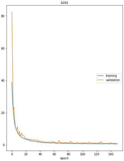
The CNN was trained using the calculated driving forces and subsidence at the PS points, and the performance of the network assessed by analysing the graphs of the cost function (MSE) for the training and validation data, as shown in Fig. 6; the root mean square error (RMSE) values of this model for the training, validation, and test data are 3.99, 8.47, and 9 mm, respectively.

Figure 6 Cost function of the training and validation data.

4.2 Comparison between CNN and traditional interpolation methods

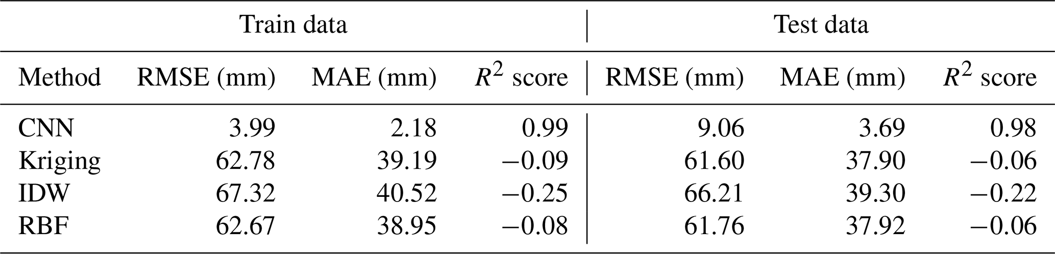
In our study, we employed four distinct methods to create a continuous subsidence surface: a CNN and three traditional interpolation methods – kriging, IDW, and RBF. The traditional interpolation methods were utilized to interpolate between PS points and calculate the subsidence across all pixels within the study area based solely on the spatial distribution of the PS points. However, these methods do not account for the subsidence driving forces, and their accuracy can be compromised by an irregular distributions of PS points.

In contrast, the CNN model was trained using subsidence driving forces to predict subsidence and generate a continuous subsidence surface. This method is particularly effective in handling irregularly distributed data points, making it suitable for scenarios where PS points are unevenly distributed across the study area. By incorporating subsidence driving forces, the CNN can provide a more reliable prediction of subsidence compared to the traditional interpolation methods. To evaluate the accuracy of these methods in predicting subsidence, we used several performance metrics, including the RMSE, MAE, and R-squared (R²), The values of these metrics for each method on the train and test data are given in Table 2. To further validate the superiority of the CNN model, we conducted statistical significance tests. A t test was performed to compare the performance metrics, with the results indicating a statistically significant improvement in the CNN model's performance over the traditional interpolation methods (p value<0.05). These results indicate a statistically significant improvement in the accuracy of the CNN compared to the traditional interpolation methods.

Table 2 Comparison of interpolation methods used to predict subsidence.

Error distribution maps are visual tools that illustrate the spatial distribution of prediction errors across the study area. These maps play a crucial role in evaluating the performance of subsidence prediction models, such as the CNN and traditional interpolation methods (kriging, IDW, and RBF).

By plotting the differences between the predicted and PSInSAR subsidence values at various locations, error distribution maps help identify patterns or areas where the models perform well or poorly. Clusters of high errors indicate that traditional interpolation methods do not perform well in areas where the range of subsidence values is greater than the average values of the entire study area and in areas with sparse PS distribution. These methods tend to have the highest errors at these points, which are often critical for accurate subsidence assessment. In contrast, the CNN demonstrates more consistent performance due to its training on subsidence driving forces, resulting in lower errors in these high-variance regions.

In our study, the error distribution maps confirmed the findings from the quantitative performance metrics (RMSE, MAE, and R² score). The CNN showed a more uniform error distribution, indicating its effectiveness in handling irregular data distributions and incorporating subsidence driving forces. This visual evidence supports the conclusion that the CNN provides a more reliable and accurate subsidence prediction compared to traditional interpolation methods (Fig. 7).

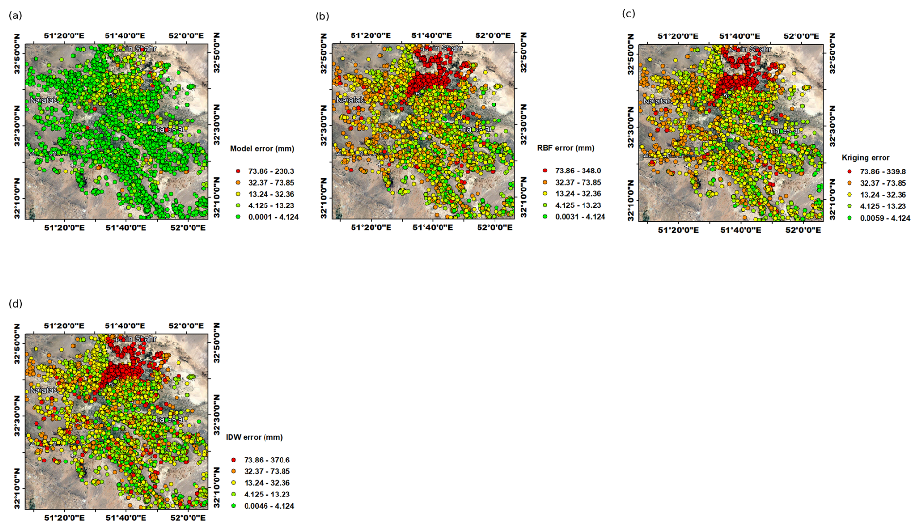
Figure 7 Error distribution map of (a) CNN, (b) RBF, (c) kriging, and (d) IDW (© Google Earth).

4.3 Subsidence of study area

In our analysis of land subsidence in the Isfahan region, we processed a total of 73 Sentinel-A images using the PSInSAR method. Through this process, we identified PS points by applying a range amplitude dispersion index threshold of 0.2 and a temporal correlation threshold of 0.8. The maximum velocity for these PS points was observed in the northeast of the study area, specifically near Shahid Beheshti Airport in Isfahan, measuring −67 mm yr⁻¹. This significant rate resulted in a cumulative displacement of approximately −33 cm in the period from 2014 to 2020 (Fig. 8).

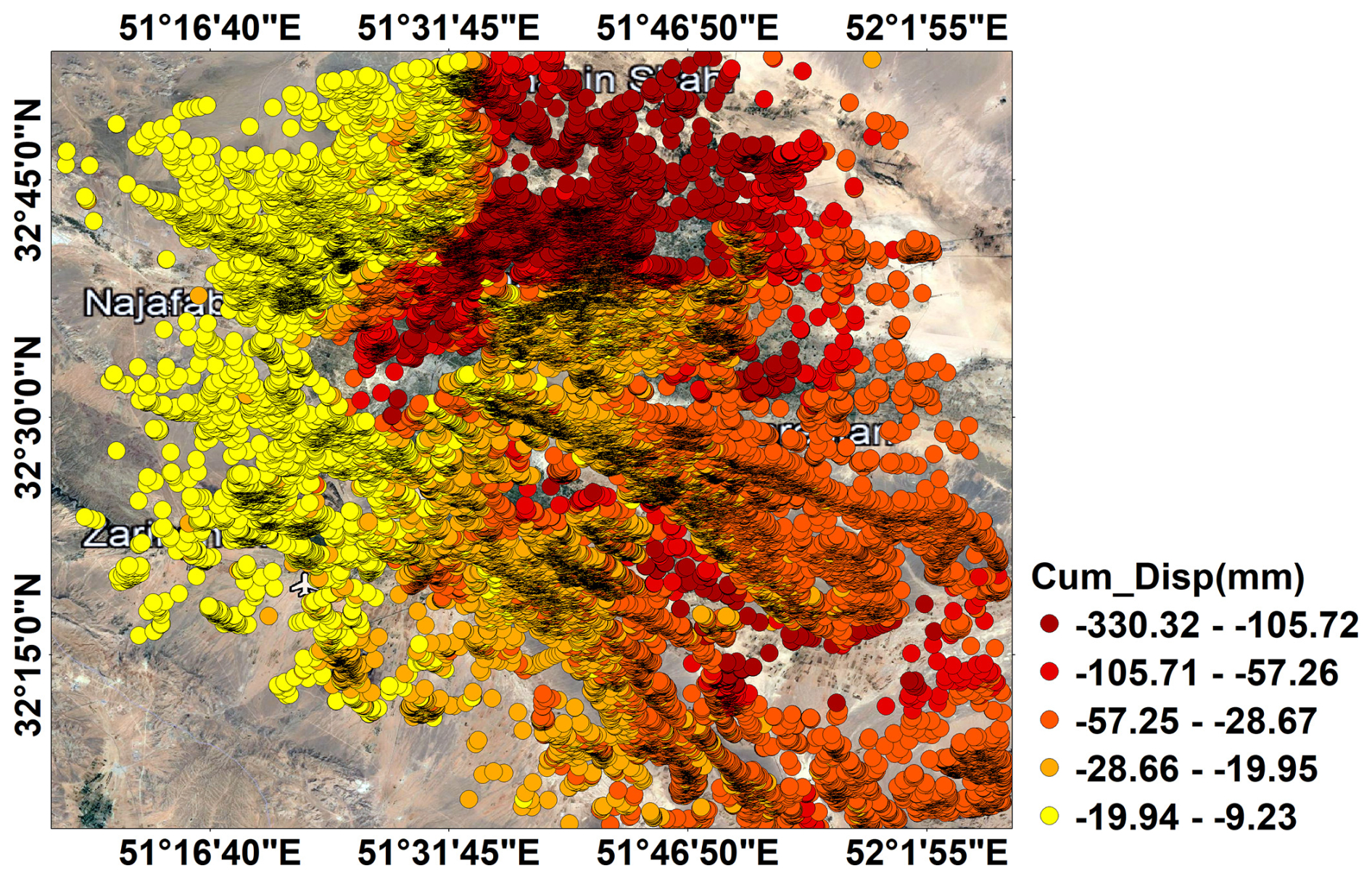
Figure 8 Cumulative displacement of PS points during the period 2014 to 2020 (© Google Earth).

A velocity map was created using kriging interpolation between PS points. The results showed that the highest velocity, approximately 67 mm yr⁻¹, was observed in the northeast of the study area (Fig. 9).

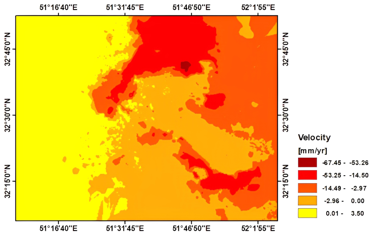
Figure 9 Velocity map using kriging.

In this research, in order to obtain a continuous subsidence surface of a specific area, two methods, kriging and CNN, have been used. The kriging method is based on mathematics and interpolation between cumulative displacement of PS points. The maximum amount of cumulative displacement obtained by the kriging method in the studied area is approximately 36 cm (Fig. 10).

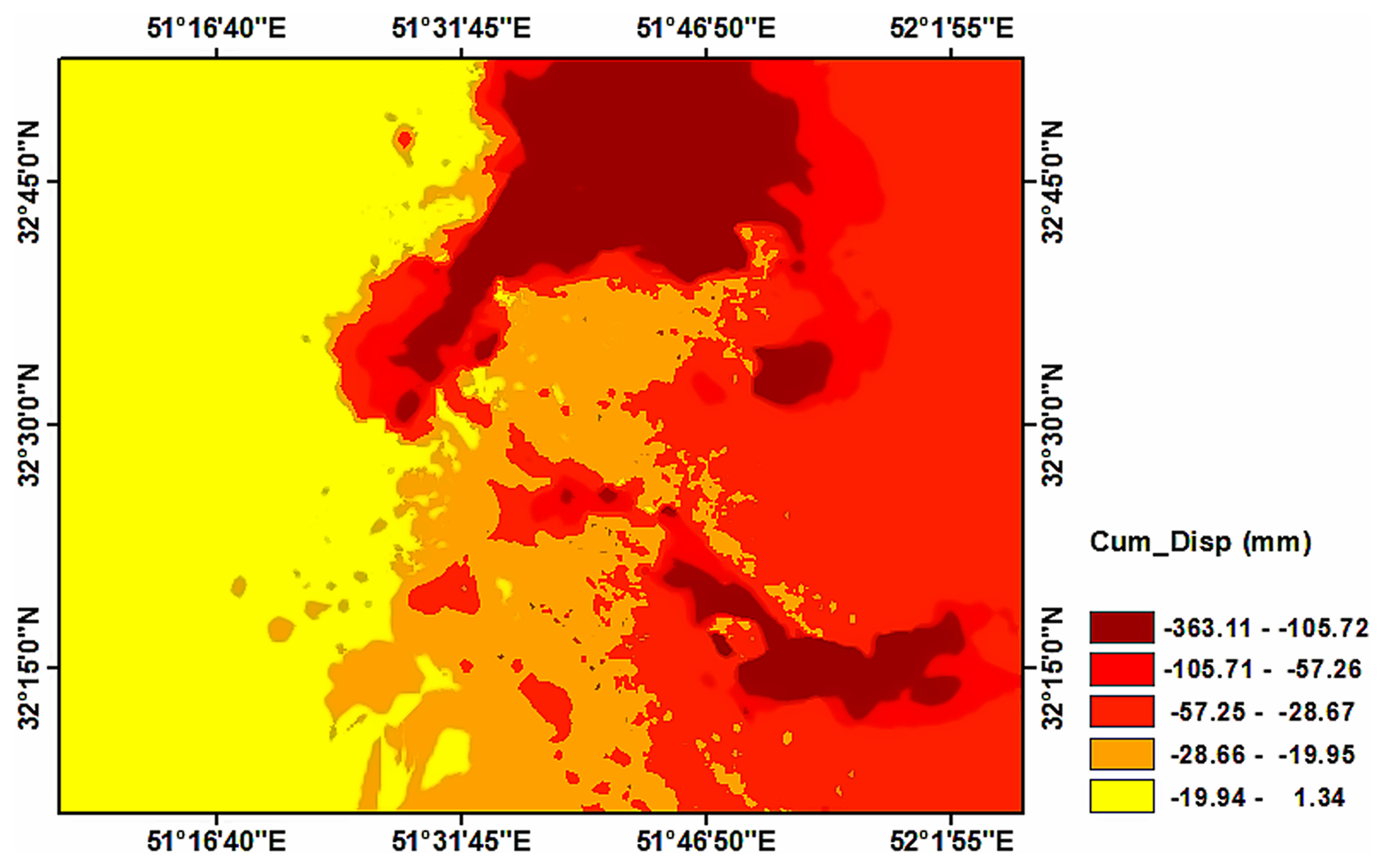
Figure 10 Cumulative displacement using kriging during the period 2014 to 2020.

The CNN model was trained with the cumulative displacement of PS points and the subsidence driving forces in these points, and finally the subsidence of the entire area was predicted with this model. The maximum amount of cumulative displacement obtained by the CNN method in the studied area is approximately 33 cm (Fig. 11).

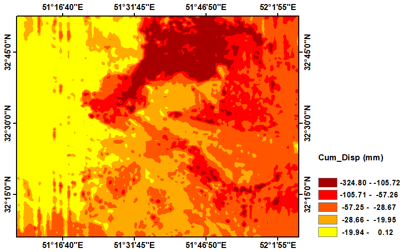
Figure 11 Cumulative displacement using CNN during the period 2014 to 2020.

Shahid Beheshti Airport in Isfahan is experiencing a critical rate of land subsidence, with an estimated velocity exceeding 45 mm yr⁻¹. This alarming rate of deformation has resulted in a significant cumulative displacement of approximately 41 cm between 2014 and 2020. Moreover, the CNN-generated subsidence map reveals a slightly higher maximum cumulative displacement of 42 cm in the region, suggesting that deep-learning models provide a more comprehensive and accurate representation of land deformation. These findings highlight the urgency of addressing subsidence-related risks, particularly in critical infrastructure areas such as airports, where even slight ground movements can lead to substantial damage. The CNN model's ability to detect and quantify subsidence in regions with sparse data further underscores its potential as a valuable tool for monitoring and mitigating land deformation across various urban and industrial settings (Fig. 12).

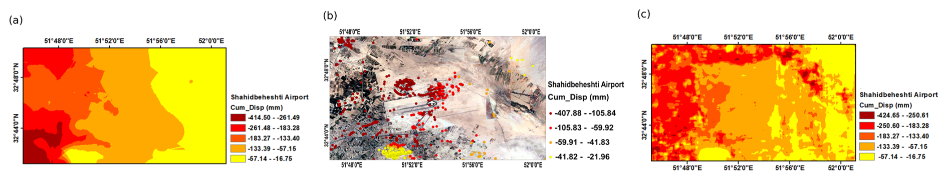
Figure 12 Cumulative displacement of Shahid Beheshti Airport during the period 2014 to 2020. (a) Continuous surface of cumulative displacement using kriging interpolation between PS points. (b) Cumulative displacement of PS points (© Google Earth). (c) Continuous surface of cumulative displacement resulting from CNN.

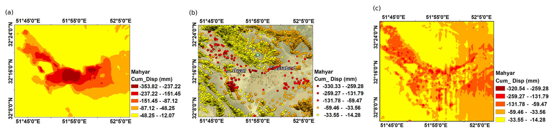
Figure 13 Cumulative displacement of Mahyar and Nasr Abad Jarqouye during the period 2014 to 2020. (a) Continuous surface of cumulative displacement using kriging interpolation between PS points. (b) Cumulative displacement of PS points (© Google Earth). (c) Continuous surface of cumulative displacement resulting from CNN.

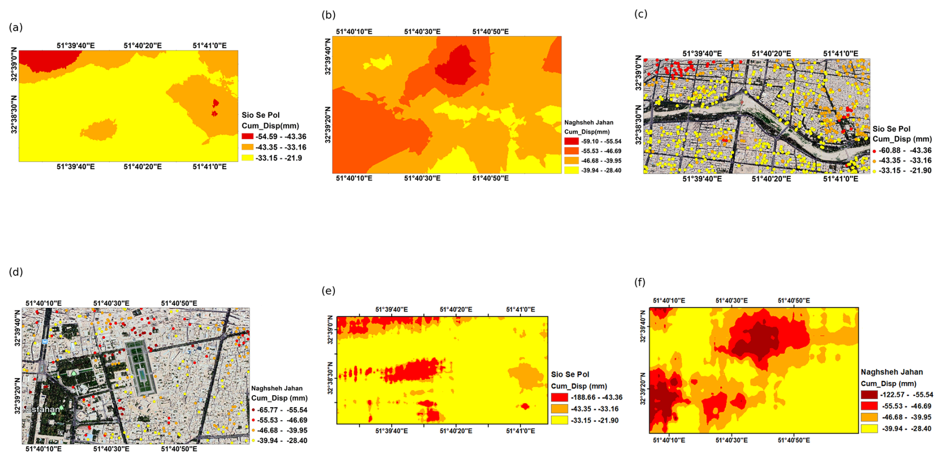
Figure 14 Cumulative displacement of (a, c, e) the Si-o-Se Pol area and (b, d, f) Naghsheh Jahan during the period 2014 to 2020. (a, b) Continuous surface of cumulative displacement using kriging interpolation between PS points. (c, d) Cumulative displacement of PS points (© Google Earth). (e, f) Continuous surface of cumulative displacement resulting from CNN.

Our study revealed significant subsidence patterns in the Mahyar and Nasr Abad Jarqouye regions, highlighting the severity of land deformation over the observation period. The analysis indicates an average subsidence velocity of approximately 5 cm yr⁻¹, leading to a substantial cumulative displacement of around 33 cm between 2014 and 2020. When applying the kriging interpolation method, the estimated maximum cumulative displacement reached approximately 35 cm. In contrast, our deep-learning-based CNN model predicted a slightly lower maximum cumulative displacement of around 32 cm. These findings underscore the variations in prediction accuracy between traditional geostatistical methods and data-driven deep-learning approaches. The discrepancy between the kriging and CNN estimates suggests that while kriging may slightly overestimate extreme displacement values due to its spatial smoothing effect, the CNN model, trained directly on observed deformation patterns, offers a more data-driven approach to subsidence prediction (Fig. 13).

In the Naghsheh Jahan area, the maximum cumulative displacements estimated using the kriging and CNN methods between 2014 and 2020 were approximately 6 and 12 cm, respectively. Similarly, in the Si-o-Se Pol area, the kriging method estimated a maximum cumulative displacement of around 6 cm, while the CNN predicted a significantly higher value of approximately 19 cm. These discrepancies highlight fundamental differences between geostatistical interpolation and deep-learning-based predictive modelling. While kriging interpolation effectively fits observed PS points, it struggles with accurate extrapolation in regions where measurement points are sparse or absent. Conversely, the CNN approach identifies significant deformation trends that kriging fails to detect, emphasizing the potential of deep-learning techniques for more reliable and spatially comprehensive subsidence prediction (Fig. 14).

The city of Khomeini Shahr is facing a concerning situation where the subsidence velocity has been estimated to be more than 45 mm yr⁻¹. Unfortunately, this has resulted in displacement in residential areas, with the maximum cumulative displacement of PS points reaching 30 cm from 2014 to 2020. According to the map generated using CNN, the maximum cumulative displacement is currently at 31 cm. A comparative analysis of kriging interpolation and the CNN model against PSInSAR observations reveals key methodological differences. The kriging interpolation method, while effective in fitting observed data points, primarily relies on mathematical interpolation and spatial smoothing. This often leads to inaccuracies in regions with a lower density of PS points, as it lacks the ability to infer displacement patterns beyond the available observations. In contrast, the CNN model estimates settlement values based on learned structural relationships, capturing complex spatial dependencies and underlying deformation mechanisms more effectively. This advantage allows the deep-learning model to provide a more continuous and spatially coherent subsidence map, improving predictive accuracy in areas with sparse measurement data (Fig. 15).

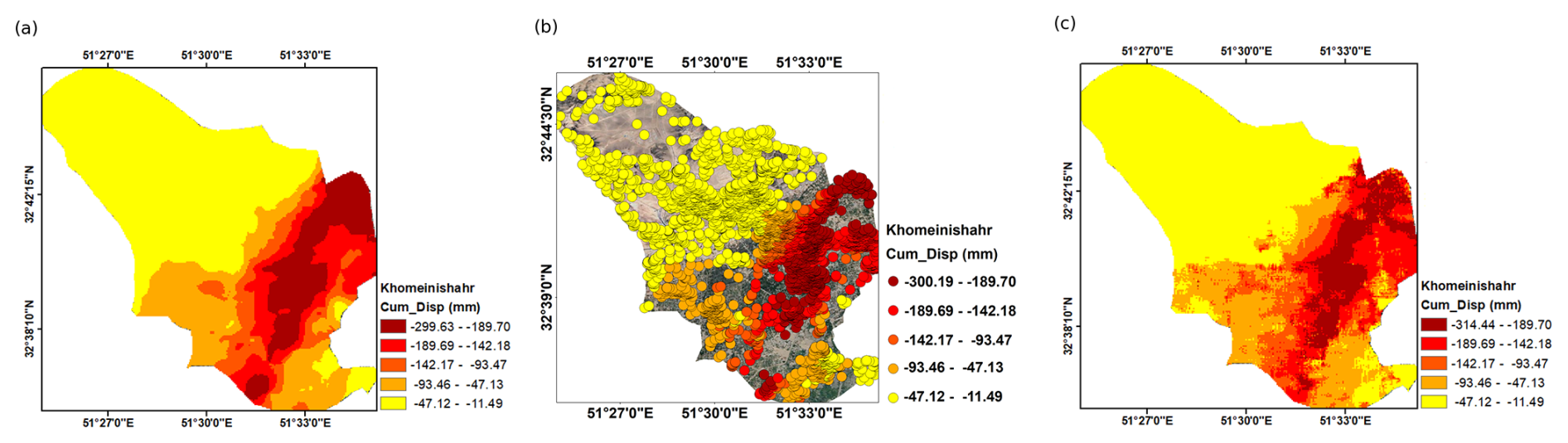
Figure 15 Cumulative displacement of Khomeini Shahr during the period 2014 to 2020. (a) Continuous surface of cumulative displacement using kriging interpolation between PS points. (b) Cumulative displacement of PS points (© Google Earth). (c) Continuous surface of cumulative displacement resulting from CNN.

In Falavarjan city, the estimated subsidence velocity exceeds 23 mm yr⁻¹, highlighting a concerning rate of land deformation. Over the period from 2014 to 2020, this has resulted in a maximum cumulative displacement of approximately 16 cm based on conventional geostatistical estimates. However, the CNN-generated subsidence map indicates a significantly higher maximum cumulative displacement of around 23 cm. The discrepancy between PSInSAR estimates and CNN predictions highlights fundamental differences in their modelling approaches. While conventional methods rely on spatial interpolation and statistical assumptions, CNNs leverage spatial dependencies and structural patterns learned from observed data, allowing for more accurate and continuous subsidence mapping. This suggests that deep-learning-based approaches may provide a more reliable representation of ground deformation, particularly in regions with a sparse distribution or absence of PS points (Fig. 16).

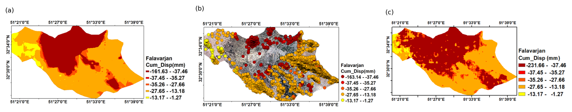
Figure 16 Cumulative displacement of Falavarjan, 2014 to 2020: (a) Continuous surface of cumulative displacement using kriging interpolation between PS points. (b) Cumulative displacement of PS points (© Google Earth). (c) Continuous surface of cumulative displacement resulting from CNN.

5 Conclusion

This study presents an innovative deep-learning framework utilizing a convolutional neural network (CNN) to generate a continuous subsidence surface across the study area. Unlike traditional methods that rely on discrete geodetic measurements, the proposed approach integrates multiple key driving factors – including NDVI, distance from wells, land use, water table depth, altitude, slope, SPI, TWI, and aspect – providing a more comprehensive and data-driven understanding of subsidence dynamics. The CNN model effectively addresses the limitations of PSInSAR, which, despite its reliability in detecting gradual land deformation, is restricted to PS points and performs poorly in vegetated or low-coherence areas. By leveraging deep learning, the proposed model enables subsidence estimation even in regions where PSInSAR measurements are unavailable, addressing a critical gap in geospatial monitoring.

The superiority of the CNN-based approach was demonstrated through a comparative analysis against conventional interpolation techniques, including kriging, IDW, and RBF. The CNN model achieved significantly lower RMSE values (3.99, 8.47, and 9 mm for the training, validation, and test datasets, respectively) and an R² score of 0.98, whereas traditional methods exhibited considerably higher RMSE values (kriging: 61.60 mm, IDW: 66.21 mm, RBF: 61.76 mm) and negative R² scores, highlighting their limitations in subsidence prediction. The study also identified severe land subsidence in key areas, with rates exceeding 45 mm yr⁻¹ at Shahid Beheshti Airport and 54 mm yr⁻¹ in the Mahyar Plain. The CNN model demonstrated an 85 % improvement in prediction accuracy over traditional methods, underscoring its robustness and effectiveness, particularly in areas with sparse and irregularly distributed data.

Despite these advancements, some challenges remain. The model's performance is influenced by the availability and quality of input data, and its computational demands necessitate the use of high-performance GPUs for efficient training. Additionally, regional variations in subsidence mechanisms may require model adaptations to ensure accuracy across diverse landscapes. Future research should focus on enhancing the model's generalizability across different geographical regions, developing real-time monitoring capabilities for early warning systems, and integrating additional datasets – such as climate variables and bedrock depth – to further refine predictive accuracy. Furthermore, exploring hybrid deep-learning architectures, such as CNN-LSTM models, may enhance computational efficiency and improve temporal prediction capabilities. Addressing these aspects will further establish deep-learning-based subsidence modelling as a scalable and effective tool for geospatial analysis, environmental monitoring, and urban planning.