Implementation of an intermediate-complexity snow-physics scheme (ISBA-Explicit Snow) into a sea ice model (SI³): 1D thermodynamic coupling and validation

Snow plays a crucial role in the formation and sustainability of sea ice. Due to its thermal properties, snow acts as an insulating layer, shielding the ice from the air above. This insulation reduces the heat transfer between the sea ice and the atmosphere. Due to its reflective properties, the snow cover also strongly contributes to albedo over ice-covered regions, which gives it a significant role in the Earth's climate system.

Current state-of-art climate models use overly simple representations of the snow cover overlaying the sea ice. The snow cover is often represented with a one-layer scheme, assuming a constant density, no wet or dry metamorphism, or that no liquid water is stored in the snow. Here we implemented an intermediate-complexity snow-physics scheme (ISBA-Explicit Snow) into a sea ice model (SI³), which serves as the sea ice component for upcoming versions of the CNRM-CM climate model. This is, to our knowledge, the first time that a snow model with such a level of complexity has been incorporated into a sea ice model designed for global to regional applications. We validated our model by comparing 1D simulations with data from the Surface Heat Budget of the Arctic Ocean (SHEBA) but also simulations from another advanced snow-on-sea ice model (SnowModel-LG), as well as simulations with the previous SI³ snow scheme.

Our model simulates realistic snow thicknesses, densities, and temperatures, aligning well with SHEBA observations and SnowModel-LG outputs, while capturing their temporal variability. We show that the thickness, density, and thermal conductivity of the snowpack are significantly affected by the choices made in parameterization for calculating snowfall density and wind-induced snow compaction and by the choice of the atmospheric forcing. Unlike the previous SI³ snow scheme that assumed constant density and thermal conductivity, our model realistically simulates the evolution of these properties, resulting in more accurate temperatures at the snow–ice interface. Ultimately, our study shows that modeling the temporal changes in the density and thermal conductivity of the snow layers leads to more realistic upper sea ice temperatures and therefore to a more accurate representation of heat transfer between the underlying sea ice and the atmosphere.

1 Introduction

Snow is an important component of the climate system. Due to its reflective properties, it regulates the Earth's energy balance. Without snow, our planet would warm due to a positive feedback loop on the ocean, land, and atmosphere system (Webster et al., 2018). In the polar regions, snow accumulates on top of the sea ice, leading to an increase in the surface albedo by up to 50 % with respect to the bare ice albedo (e.g., Perovich and Polashenski, 2012) and to a reduction of the solar radiation absorbed by the sea ice (and thus the climate system). Conversely, snow on sea ice acts as an insulator (e.g., Sturm and Massom, 2017), reducing the heat transfer between the sea ice and the atmosphere and delaying the ice thermodynamic thickening, keeping the ice warm and thus thin (Fichefet et al., 2000; Lecomte et al., 2013). Snow can also promote sea ice growth through the formation of superimposed ice (the refreezing of fresh percolating meltwater on top of sea ice; Nicolaus et al., 2003) and snow ice (refrozen mixture of snow and saltwater flooding the base of the snow; Jutras et al., 2016). Despite its importance, snow on sea ice remains an understudied component of the climate system.

The optical and thermal properties of snow are influenced by a multitude of processes that vary significantly in their frequency, magnitude, and occurrence across seasons, regions, and hemispheres (see Webster et al., 2018, and Sturm and Massom, 2017, for recent reviews). At microscopic scale, the freshly deposited snow undergoes complex metamorphic processes that modify its grain size, shape, and density, thus impacting its thermal conductivity (Sturm et al., 1997) and albedo (Bohren and Beschta, 1979). After snowfall, the wind erodes or drifts the unconsolidated snow, shaping the heterogeneity of the snow cover in accordance with the sea ice topography. Some of this blowing snow may also fall into leads, open cracks, or polynyas where it may melt, form slush, or refreeze (Leonard and Maksym, 2011). Wind also tends to compact the snowpack, thus increasing its density (Sommer et al., 2018).

Accurately representing snow on sea ice in climate models is crucial for capturing the complex interactions and feedbacks within the climate system and for ensuring more reliable predictions of future climate changes (Fichefet et al., 2000; Holland et al., 2021; Lecomte et al., 2013). For instance, Fichefet et al. (2000) showed that reducing by half the thermal conductivity of the snow overlaying the Antarctic sea ice in a global coarse-resolution ice–ocean model significantly decreases the sea ice thickness. They also observed changes in the stratification of the Southern Ocean and a weakening of the Antarctic Bottom Water meridional overturning. Similarly, in the Arctic, Lecomte et al. (2013) showed that using a constant snow conductivity in a coupled sea ice–ocean model leads to an overestimation of sea ice thickness in the Arctic. More recently, Holland et al. (2021) showed that increasing snow precipitation in climate models results in significant changes to sea ice thickness, emphasizing the critical need for an accurate representation of the snow cover on sea ice within coupled Earth system models.

While current state-of-the-art climate models employ relatively complex snow schemes over land, the scarcity of observations and the technical challenges involved in coupling snow with sea ice (Liston et al., 2020) lead to relying on overly simplistic representations of the snow on sea ice. Indeed, snow on sea ice in climate models is typically depicted using a simplified one-layer scheme, assuming constant snow density and thermal conductivity, without taking into account liquid water retention or snow metamorphism.

Over recent years, efforts have been made towards using more complex snow models over the sea ice. These models are mainly designed to produce datasets of snow properties such as (primarily) its thickness or (secondarily) density to compensate for the lack of observational data and/or assist with remote sensing (the snow thickness is a required input to derive the sea ice thickness from satellite altimetry). For example, Liston et al. (2020) developed for such applications a Lagrangian snow model (SnowModel-LG) which follows the ice motion and includes a representation of snow density and grain size evolution, blowing-snow sublimation, snowmelt, and superimposed ice formation. Similarly, Wever et al. (2020) developed a sea ice module for the unidimensional, physics-based, detailed, multi-layer snow cover model SNOWPACK, which they used in a Lagrangian framework.

Such Lagrangian models are useful to improve the knowledge of the interactions between snow and sea ice but are not suitable for climate systems that use an Eulerian framework. Simple modeling of snow on sea ice with an Eulerian framework has also been achieved. Lecomte et al. (2013) developed a parameterization that consists of a set of two linear equations relating the snow thermal conductivity and density to the mean seasonal wind speed. More recently, Petty et al. (2018) developed an Eulerian model which uses two snow layers, a rather simple parameterization representing accumulation, wind packing, advection–divergence, and blowing snow lost to leads to represent key sources and sinks of snow on sea ice. In the CICE sea ice model (Hunke et al., 2017), snow physics are handled by the Icepack component (Shapero et al., 2021), which includes some advanced parameterizations such as wind-driven snow erosion and compaction. In this scheme, an effective snow density is diagnosed based on wind speed and used to limit erosion of denser snow layers. Additionally, the model parameterizes the snow grain size evolution as a function of temperature gradients and density, which in turn influences surface albedo.

The sea ice component for upcoming versions of the CNRM climate model (CNRM-CM, Voldoire et al., 2013), called SI³ (Sea Ice modeling Integrated Initiative, Vancoppenolle et al., 2023), incorporates a simplistic representation of snow over sea ice, assuming a constant density, thermal conductivity, and albedo. In this study, we integrate a more advanced snow scheme, ISBA-Explicit Snow, (ISBA-ES, Boone and Etchevers, 2001), into SI³ to improve its representation of the snow over sea ice. The ISBA-ES snow model incorporates detailed representations of snowpack properties such as density, grain size, and thermal conductivity, allowing for more accurate simulation of snow accumulation, compaction, metamorphism, and melt processes than previous snow schemes within SI³. To the best of our knowledge, this is the first time a snow-physics scheme of this level of complexity has been integrated into a global sea ice model.

Here, we present the SI³ + ISBA-ES model, the developments made to allow the integration of ISBA-ES within the SI³ framework, and the validation of our coupled model in a unidimensional context focusing on the thermodynamic processes only (i.e., without representing the effects of sea ice dynamics). To achieve this, we decided to validate our model using Lagrangian data from the Surface Heat Budget of the Arctic Ocean (SHEBA) experiment (Perovich et al., 1999), where there are no direct effects of sea ice drift on snow properties, and against SnowModel-LG (Stroeve et al., 2020) data.

2 Materials and method

2.1 Sea ice model

The sea ice model used is SI³ (Sea Ice modeling Integrated Initiative, Vancoppenolle et al., 2023), which is part of the Nucleus for European Modelling of the Ocean (Madec and the NEMO System Team, 2024) in its version 4.2.2. The core of SI³ integrates a suite of physical processes crucial for accurately simulating sea ice evolution. These processes include thermodynamics, where heat exchanges between the atmosphere, ocean, and ice drive ice growth and melt. Additionally, SI³ accounts for mechanical forces such as ice deformation and ridging, which significantly impact ice thickness distribution and overall sea ice morphology. The sea ice thermodynamics are modeled using a 1D scheme that conserves energy (Bitz and Lipscomb, 1999) and includes a time-dependent salinity profile (Vancoppenolle et al., 2009). SI³ resolves a subgrid-scale sea ice thickness distribution (Bitz et al., 2001; Thorndike et al., 1975). As the paper focuses on thermodynamics, we use the SI³ model in 1D (vertical) configurations, with only one sea ice category and two ice layers, assuming that the dynamical processes affecting the snow and sea ice such as the ice deformation and ridging are negligible and that the advection is accounted by following the trajectory of the observations used to validate the model (see Sect. 2.4). Since we focus on the period where the snow is present, we neglect melt ponds over sea ice in our configurations.

The surface forcing is computed by the NEMO bulk algorithm (NCAR; Large and Yeager, 2004). Turbulent heat fluxes over sea ice are computed from 2 m air temperature and humidity, 10 m winds, and surface pressure. In the current version of the model, the snow fraction is either 1 or 0, meaning that we assume that the snow covers the whole ice fraction.

2.2 Snow model

The original version of the SI³ model used for this paper, prior to any snow model implementation, simulates the snow cover assuming constant density (330 kg m⁻³) and thermal conductivity (0.31 $\mathrm{W}{\mathrm{m}}^{-\mathrm{1}}{\mathrm{K}}^{-\mathrm{1}}$), no liquid water stored in snow, and no snow metamorphism. When SI³ is hereafter coupled with the ISBA-ES snow model (see Sect. 2), the snow cover is simply computed by ISBA-ES instead of the original SI³ trivial snow scheme.

The ISBA-Explicit Snow (ISBA-ES) snow model (Interactions between Soil Biosphere Atmosphere-Explicit Snow) was developed by Boone and Etchevers (2001) and revised by Decharme et al. (2016) (see also the user manual, Boone, 2002). Initially developed for alpine conditions, it incorporates detailed representations of snowpack properties such as density, grain size, and thermal conductivity and accounts for complex processes like snow accumulation, compaction, dry and wet metamorphism, liquid water storage, and melt processes. The model is based on similar schemes as described by Kondo and Yamazaki (1990), Loth et al. (1993), Lynch-Stieglitz (1994), and Sun et al. (1999). We use 12 snow layers for our simulations. The number of vertical layers is fixed but their thickness is adapted at each time step to the total snow thickness, and the ISBA-ES prognostic variables are remapped at each time step on the ISBA-ES vertical grid. At each time step, the snow layer thickness is updated according to the total snow thickness. The upper layer thickness is bounded so that its thickness does not exceed 0.2 m in order to resolve the diurnal cycle based on an assumed thermal damping depth of snow (Boone and Etchevers, 2001). Thickening beyond that threshold ultimately results in snow transfer toward the layers below. The prognostic variables of the model are the snow heat content, the snow density, the snow thickness, and the snow albedo. ISBA-ES includes parameterizations for processes like snow sublimation, blowing-snow transport, and snowfall density, enabling a comprehensive understanding of the physical mechanisms driving the snowpack evolution. The snow metamorphism is not explicitly computed but is accounted for in the density and albedo parameterizations.

2.2.1 Snow density

The local rate of change of snow density ρ_s is parameterized after Brun et al. (1989, 1997):

$$\begin{array}{}\text{(1)}& {\displaystyle \frac{\partial {\mathit{\rho }}_{\mathrm{s}}}{\partial t}}={\displaystyle \frac{{\mathit{\sigma }}_{\mathrm{s}}}{{\mathit{\eta }}_{\mathrm{s}}(T_{\mathrm{s}},{\mathit{\rho }}_{\mathrm{s}})}}+{\mathit{\xi }}_{\text{wind}}.\end{array}$$

The first term on the right-hand side represents the snow overburden (the compactive viscosity term). It accounts for the pressure of the snow above (σ_s, in Pa) and its viscosity (η_s, in Pa s), determined by snow temperature T_s and density ρ_s (Kojima, 1967; Mellor, 1964). The second, term ξ_wind, represents the effect of the wind compaction (see Sect. 2.2.3).

2.2.2 Energy balance and heat flow

The heat content H_s (in J m⁻²) or energy needed to melt each snow layer is defined using an expression similar to those of Lynch-Stieglitz (1994) and Sun et al. (1999) as

$$\begin{array}{}\text{(2)}& H_{\mathrm{s}}=c_{\mathrm{s}}{h}_{\mathrm{s}}(T_{\mathrm{s}}-T_{\mathrm{f}})-L_{\mathrm{f}}(W_{\mathrm{s}}-W_{\mathrm{l}}),\end{array}$$

where h_s is the snow thickness, L_f is the latent heat of fusion, c_s is the snow heat capacity defined following Verseghy (1991), W_s is the snow water equivalent (SWE), and W_l is the snow liquid water content. The heat content is used to diagnose the snow temperature using the equation above assuming that there is no liquid water in the snow layer (W_l=0).

$$\begin{array}{}\text{(3)}& T_{\mathrm{s}}=T_{\mathrm{f}}+{\displaystyle \frac{H_{\mathrm{s}}+L_{\mathrm{f}}{W}_{\mathrm{s}}}{c_{\mathrm{s}}{h}_{\mathrm{s}}}}\end{array}$$

If the calculated temperature exceeds the freezing point, it is set to T_f, and the liquid water content is determined from the heat content equation as follows:

$$\begin{array}{}\text{(4)}& W_{\mathrm{l}}=W_{\mathrm{s}}+{\displaystyle \frac{H_{\mathrm{s}}}{L_{\mathrm{f}}}}.\end{array}$$

The layer-averaged snow temperature equation (T_s,k) for the snow layer k is then expressed as

$$\begin{array}{}\text{(5)}& c_{\mathrm{s},k}{D}_{\mathrm{s},k}{\displaystyle \frac{\partial T_{\mathrm{s},k}}{\partial t}}=G_{\mathrm{s},k-\mathrm{1}}-G_{\mathrm{s},k}-F_{\mathrm{s},k},\end{array}$$

where F_s represents latent heat absorption or release due to phase changes (between water and ice). The heat flux G_s is simply expressed as

$$\begin{array}{}\text{(6)}& G_{\mathrm{s}}=J_{\mathrm{s}}+Q_{\mathrm{s}},\end{array}$$

where J_s and Q_s are the heat conduction and radiation fluxes, respectively. Q_s is computed as follows:

$$\begin{array}{}\text{(7)}& Q_{\mathrm{s},i}=R_{\mathrm{g}}(\mathrm{1}-\mathit{\alpha })\exp (-{\mathit{\nu }}_{\mathrm{s},k}{h}_{\mathrm{s},k})k_{\mathrm{s}},\end{array}$$

where R_g is the incoming shortwave radiation at the snow surface, α is the albedo, and ν_s,k is the shortwave radiation extinction coefficient (Bohren and Barkstrom, 1974). The extinction coefficient γ_s,i at each snow level i is computed as in Anderson (1976) and depends on the snow optical diameter d_s,i such as ${\mathit{\gamma }}_{\mathrm{s},i}=C_{\mathrm{v}}{\mathit{\rho }}_{\mathrm{s},i}{d}_{\mathrm{s},i}^{-\mathrm{1}/\mathrm{2}}$. The snow optical diameter is itself parameterized after Anderson (1976) and depends on the snow density as $d_{\mathrm{s},i}=\text{MIN}(d_{\mathrm{s},\text{max}},a_{\text{sd}}{b}_{\text{sd}}{\mathit{\rho }}_{\text{si}}^{\mathrm{4}})$, where d_s,max is the maximum grain size authorized and is equal to 2.796 × 10⁻³ m. The snow albedo is solved over three bands (ultraviolet and visible, 0.3–0.8 µm; two near-infrared bands, 0.8–1.5 µm and 1.5–2.8) as in Decharme et al. (2016, Eq. 17) and is a function of the snow optical diameter and of the age of the first layer of the snowpack. The conduction flux J_s is computed as follows:

$$\begin{array}{}\text{(8)}& J_{\mathrm{s},i}={\displaystyle \frac{\mathrm{2}{k}_{\mathrm{s},k}(T_{\mathrm{s},k}-T_{\mathrm{s},k+\mathrm{1}})}{h_{\mathrm{s},k}+h_{\mathrm{s},k+\mathrm{1}}}},\end{array}$$

where h_s,k is the snow layer thickness, and k_s is the snow thermal conductivity. Finally, the net heat flux G_s,0 at the atmosphere–snow interface is expressed as

$$\begin{array}{}\text{(9)}& \begin{array}{rl}{G}_{\mathrm{s},\mathrm{0}}& =R_{\mathrm{g}}(\mathrm{1}-\mathit{\alpha })+{\mathit{\epsilon }}_{\mathrm{n}}{R}_{\text{at}}-\mathit{\sigma }{T}_{\mathrm{s},\mathrm{1}}^{\mathrm{4}}-H-\text{LE}\\ & +P_{\text{rn}}{C}_{\mathrm{w}}(T_{\text{al}}-T_{\mathrm{f}}),\end{array}\end{array}$$

where ε_n is the snow emissivity (assumed to be 1), R_at is the downwelling atmospheric longwave radiation, σ is the Stefan–Boltzmann constant, and H and LE are the sensible and latent heat fluxes. The last term on the right-hand side of the equation above is a precipitation advection term where c_w represents the specific heat of water, P_rn is the rainfall rate, and T_al is the temperature of rainfall, assumed to be the air temperature if it is above the temperature of fusion T_f.

2.2.3 Parameterizations

ISBA-ES uses parameterizations to represent various processes, including the changes in snow albedo, grain size, radiation extinction coefficient, compactive viscosity (that represent the snow overburden), thermal conductivity, snowfall density, and snow compaction due to wind (see Sects. 2.2.1 and 2.2.2). For the purposes of this study, some of the parameterizations were adjusted to better suit polar conditions. Thus, this section only outlines the parameterizations that differ from the standard ISBA-ES configuration as described by Decharme et al. (2016). Detailed descriptions of the parameterizations that remained unchanged from the default ISBA-ES configuration for this study are available in Boone and Etchevers (2001) and Decharme et al. (2016).

Snowfall density

The density of the snow precipitation is parameterized as in Pahaut (1975):

$$\begin{array}{}\text{(10)}& {\mathit{\rho }}_{\text{new}}=A_{\text{sn}}+B_{\text{sn}}(T_{\mathrm{a}}-T_{\mathrm{f}})+C_{\text{sn}}(V_{\mathrm{a}}{)}^{\mathrm{1}/\mathrm{2}},\end{array}$$

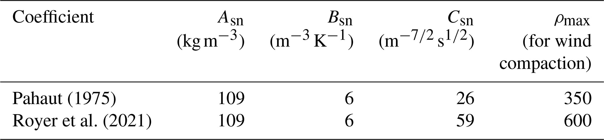
where T_a is the air temperature, T_f is the temperature of fusion, and V_a is the 10 m wind speed. A_sn, B_sn, and C_sn are coefficients given by Pahaut (1975). Additionally, we tested another set of values for these coefficients, supposedly more suitable to the Arctic region given by Royer et al. (2021). The values of the coefficients are listed in Table 1.

Table 1 Coefficients used for the parameterization of the snowfall density.

Wind compaction

The snowpack density is increased by the wind compaction processes. In ISBA-ES, the snowdrift ξ_wind (i.e., the wind compaction) is computed as

$$\begin{array}{}\text{(11)}& {\mathit{\xi }}_{\text{wind}}={\displaystyle \frac{\partial {\mathit{\rho }}_{\mathrm{s},k}}{\partial t}}={\displaystyle \frac{{\mathit{\rho }}_{\text{max}}-{\mathit{\rho }}_{\mathrm{s},k}}{{\mathit{\tau }}_{\mathrm{i}}}},\end{array}$$

where k denotes the snow layer, ρ_max is a maximum snow density authorized, and τ_i is the time characteristic for snow grain change under wind transport and is computed as

$$\begin{array}{}\text{(12)}& {\mathit{\tau }}_k={\displaystyle \frac{\mathit{\tau }}{{\text{Wind}}_{\text{Effect}}{\mathrm{\Gamma }}_{k,\text{drift}}}},\end{array}$$

where τ is empirically set to 48 h, Wind_Effect is an empirical coefficient on wind effect, and Γ_k,drift represents the grain driftability with an exponential decay function of the depth of the snow layer. In our experiments, we use two sets of values for the parameters ρ_max and Wind_Effect. The first one is the default parameters used in ISBA-ES, defined by Brun et al. (1997), where ρ_max = 350 g m⁻³ and Wind_Effect = 1, and the second one is the parameters defined by Royer et al. (2021), where ρ_max = 600 g m⁻³ and Wind_Effect = 1.5, in order to increase the effect of the wind on compaction and improve the representation of the upper wind slab layer typical of Arctic snowpacks (e.g., Domine et al., 2018; Sturm et al., 2002, and references therein).

Thermal conductivity

In the default version of ISBA-ES, the thermal conductivity is computed as in Anderson (1976). However, this parameterization may not be suited to the Arctic region. For this reason, and to be consistent with the SnowModel-LG model used for comparison and validation (Liston et al., 2020, and see Sect. 2.4), we implemented the Sturm et al. (1997) parameterization for the thermal conductivity, which is computed as follows:

$$\begin{array}{}\text{(13a)}& k_{\mathrm{s}}=\mathrm{0.138}-\mathrm{1.01}\mathit{\rho }+\mathrm{3.233}{\mathit{\rho }}^{\mathrm{2}}\mathrm{0.156}\le \mathit{\rho }\le \mathrm{0.6}\end{array}$$

and

$$\begin{array}{}\text{(13b)}& k_{\mathrm{s}}=\mathrm{0.023}+\mathrm{0.234}\mathit{\rho }\mathit{\rho }\le \mathrm{0.156}.\end{array}$$

2.3 Snow and ice coupling

In this work, we couple the ISBA-ES model to the SI³ model so that most snow thermodynamic processes are not computed anymore by the original SI³ snow scheme but by ISBA-ES. However, some sea-ice-related processes (not accounted for in the ISBA-ES original model) such as the snow–ice formation are not resolved by the current version of ISBA-ES and are still resolved within the sea ice model. The coupling is made online, meaning that the ISBA-ES code is incorporated within SI³ and no coupler is needed. However, in the present version of the code the interactions of the snow with the sea ice dynamics and with the melt ponds are not yet implemented so we focus on evaluating the thermodynamic part of the coupling.

At the beginning of a time step, the lower boundary condition of ISBA-ES is given by the temperature and the thermal conductivity of the upper sea ice layer. After the resolution of snow processes, the conduction flux at the snow–ice interface computed by ISBA-ES is sent to SI³ and is used as upper boundary condition for the temperature solving in the sea ice. Note that since the snow–ice conversion is computed within SI³ and not ISBA-ES, the vertical profiles of the ISBA-ES prognostic variables are also exchanged between the two models and updated in both ISBA-ES (due to “snow-only” processes) and SI³ (due to snow–ice conversion).

The conduction flux at the snow–ice interface F_c is recomputed in ISBA-ES as $F_{\mathrm{c}}=-K_{\mathrm{s}-\mathrm{i}}\cdot (T_{i,\mathrm{1}}-T_{\mathrm{s},N})$, where T is the temperature, the subscripts i and s, N denote the ice or the snow and the index 1, and N denotes the upper layer and the lower layer, respectively. K_s-i is the thermal conductivity at the snow–ice interface, which is computed as in SI³ and Rousset et al. (2015): $K_{\text{s-i}}=\frac{(h_{\mathrm{s},N}+h_{i,\mathrm{0}})\cdot (k_{i,\mathrm{0}}\cdot k_{\mathrm{s},N})}{(k_{i,\mathrm{0}}\cdot h_{\mathrm{s},N}+k_{\mathrm{s}}\cdot h_{i,\mathrm{0}})}$, where k is the thermal conductivity and h is the thickness of the corresponding layer (depending on the subscript).

The ISBA-ES model is called just before the resolution of the sea ice thermodynamic processes. The basic iteration procedure for the SI³ + ISBA-ES model follows the steps below.

• The ISBA-ES model is called. The model reads its prognostic variables (snow thickness, density, heat content, and albedo) from a restart or from a previous time step and the temperature and conductivity of the first sea ice layer from current time step. Then, it computes the changes in snow thickness, heat content, and density due to snowfall and remaps the prognostic variables on its vertical grid. Then, the model resolves the evolution of prognostic variables accounting for processes such as settling, compaction, metamorphism, and melting. Additionally, it calculates the conduction flux at the interface between the snow and sea ice and the radiative flux transferred to the sea ice below. At the end of the ISBA-ES iteration, the vertical profiles of ISBA-ES prognostic variables along with any remaining heat and evaporation flux to be transmitted to SI³ (if all snow has melted during a time step) are stored.

• The conduction flux at the interface between the snow and the sea ice estimated by ISBA-ES is then used as a boundary condition to solve the temperature equation in the sea ice by SI³, and changes in ice thickness due to ice melt are computed by SI³ as well.

• If the snow exceeds a certain thickness and density so that the snow base is pushed below the freeboard, snow–ice formation occurs, and the vertical profiles of snow and sea ice thickness and enthalpy are updated and saved for use in the next time step.

Note that the current version of the SI³ + ISBA-ES model does not yet account for the dynamic processes related to the sea ice advection and deformation and thus cannot be used to perform realistic 3D simulations. Nonetheless, the version of the model presented here is already suitable for 1D simulations on multiyear ice, following the ice motion.

2.4 Validation data

We use the data collected during the Surface Heat Budget of the Arctic Ocean (SHEBA) experiment to validate our model (Perovich et al., 1999). The SHEBA experiment took place from 1997 to 1998. During this period, several snow variables useful to validate our model such as the snow thickness, the snow surface temperature, and the snow–ice interface temperature were collected daily. Snow thicknesses were gathered by employing magnaprobes and ruler measurements along transects ranging from 200 to 500 m in length. We used the same SHEBA snow thickness dataset as Stroeve et al. (2020), where in situ observations were aggregated over all transects and averaged for each day. Since most snow measurement were taken on multiyear ice (Sturm et al., 2002), the snow depth averaged over all transects can be approximated as the snow depth on level ice. Additionally, the snow surface temperature and the snow–ice interface temperature were collected from thermistors as described in Persson et al. (2002). Note that the two temperatures were not measured exactly at the same exact location, leading to an uncertainty of ∼ 0.6 °C in the temperatures.

We also compared our model with the outputs of the SnowModel-LG simulations performed by Liston et al. (2020) and Stroeve et al. (2020). SnowModel-LG is a multi-layer model specifically designed to simulate the key physical processes governing the seasonal evolution of snow thickness and density over sea ice. It operates on a Lagrangian framework and incorporates various parameterizations to account for processes like blowing-snow redistribution, sublimation, changes in density and grain size, and snow metamorphism. More details about the model can be found in by Liston et al. (2020) and Stroeve et al. (2020). The model is forced either by NASA's Modern Era Retrospective Analysis for Research and Applications Version 2 (MERRA-2, Gelaro et al., 2017) or by the European Centre for Medium-Range Weather Forecasts (ECMWF) atmospheric data (ERA5, Hersbach et al., 2020). Approximately 61 000 Lagrangian parcels were simulated with this model over the Arctic, covering the 1980–2018 period. We also use the SnowModel-LG data described in Stroeve et al. (2020), which gives an estimate of the classic behavior of a snow model of intermediate complexity. To compare SnowModel-LG with our simulations over the SHEBA site, we used the same Lagrangian parcel used in Stroeve et al. (2020), which is a representative parcel located initially near the departure location of the SHEBA campaign (see Sect. 3.1 in their paper). The path of the SHEBA experiment is illustrated in Fig. 1.

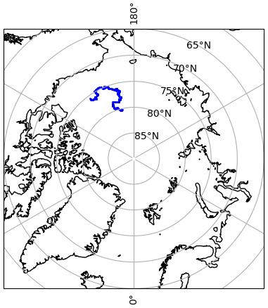
Figure 1 Trajectory of the SHEBA experiment during the observation period (blue).

More recent campaigns than SHEBA have measured snow over sea ice over nearly year-long periods, notably the MOSAiC campaign (Nicolaus et al., 2022). However, cumulative snowfall during MOSAiC showed significant variability across transects – up to 10 times higher than the mean in some cases – due to intense blowing-snow events (Wagner et al., 2022). In contrast, SHEBA reported only a 30 % increase in snow depth over ridges (Sturm et al., 2002). Additionally, the average cumulative snowfall across all MOSAiC transects was relatively low, ranging from 72 to 107 mm SWE, with a peak snow depth of 30 cm (Itkin et al., 2023). This contrasts with the SHEBA campaign, where cumulative snowfall reached around 179 mm SWE and snow depth peaked at 42.3 cm, with an average of 37.3 cm (Sturm et al., 2002). For these reasons, we chose to use the SHEBA dataset instead of MOSAiC to validate our model.

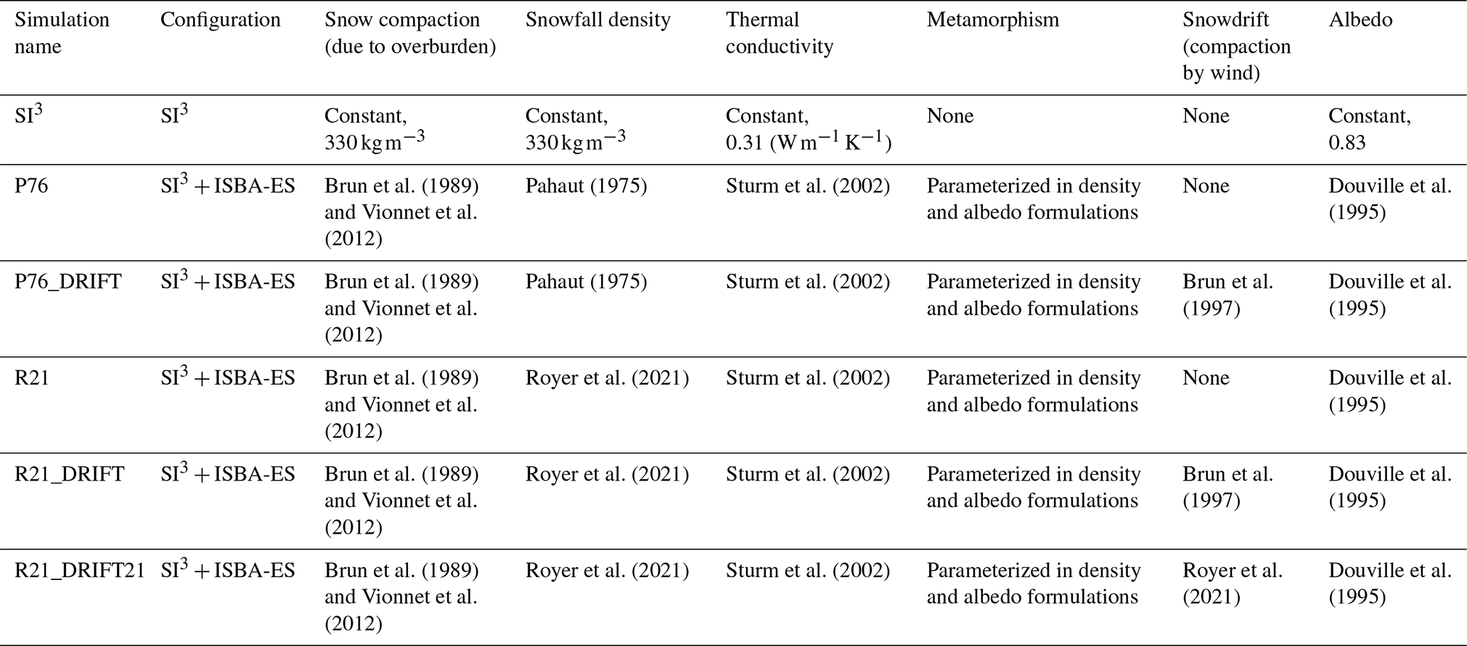
Table 2 Parameterizations used to represent snow processes in all SI³ + ISBA-ES (and SI³-only) simulations.

2.5 Configurations

Among all the parameterizations available in ISBA-ES, the parameterizations of the snowfall density and of the wind-induced compaction are the ones with the greatest impact on the snow thickness and density. Thus, we performed a set of experiments to evaluate the sensitivity of the model to these parameterizations. Two experiments, P76 and R21 using the Pahaut (1975) and Royer et al. (2021) coefficients (see Sect. 2.2.3) for the parameterization for the snowfall density, respectively, were conducted without the snowdrift parameterizations active. Additionally, two similar experiments, P76_DRIFT and R21_DRIFT, were conducted with the snowdrift parameterization enabled, using the Pahaut (1975) and Royer et al. (2021) coefficients, respectively, for snowfall density parameterization. Another experiment, named R21_DRIFT21, was set up using the Royer et al. (2021) coefficients for both snowfall density and snowdrift parameterization (see Sect. 2.2.3). Lastly, we prepared a configuration called SI³, where the snowpack is simulated by SI³ in its NEMO 4.2 stable version (i.e., without ISBA-ES) to examine the differences in snow state simulation between SI³-only and SI³ + ISBA-ES. The parameterizations used in these experiments are summarized in Table 2.

SI³ is used in sea-ice-only mode, meaning that the sea ice and snow component is forced from both oceanic and atmospheric sides. We use the GLORYS12 (Lellouche et al., 2018) reanalysis as forcing data for the ocean and either the MERRA-2 or ERA5 reanalysis for the atmosphere (more information is provided in the Results section). To force our simulations, we followed the trajectory of the SHEBA tower and extracted the forcing data at the position of the tower for each day.

The simulations were initialized on 3 November 1997. We use the SHEBA snow thickness averaged over all snow transects for this date (0.153 m) as the initial value for our model. We also use the SnowModel-LG density for this date (191 kg m⁻³ ) to initialize ISBA-ES simulations since the density for SHEBA was not measured on this date. For the sea ice thickness and concentration, we use the GLORYS12 value for this date (2.95 m and 0.88, respectively).

3 Results

3.1 Validation at the SHEBA site

3.1.1 Sensitivity to the atmospheric forcing

Following Stroeve et al. (2020), we first investigate the effect of the atmospheric forcing on the snowpack variability. For this, we conducted two simulations using the P76_DRIFT setup, changing only the atmospheric forcing applied – either ERA5 or MERRA-2 – over the duration of the SHEBA experiment (Perovich et al., 1999), following the tower trajectory. We compare the results obtained from our simulations with the SHEBA data and with the outputs available from the SnowModel-LG simulations from Liston et al. (2020) and Stroeve et al. (2020). While the resolution disparity between our model's estimates (roughly equivalent to the resolution of the forcing, 31 km for ERA5) and the point measurements from SHEBA prevents a quantitative assessment of our simulations, it does provide an estimate of the simulation's realism.

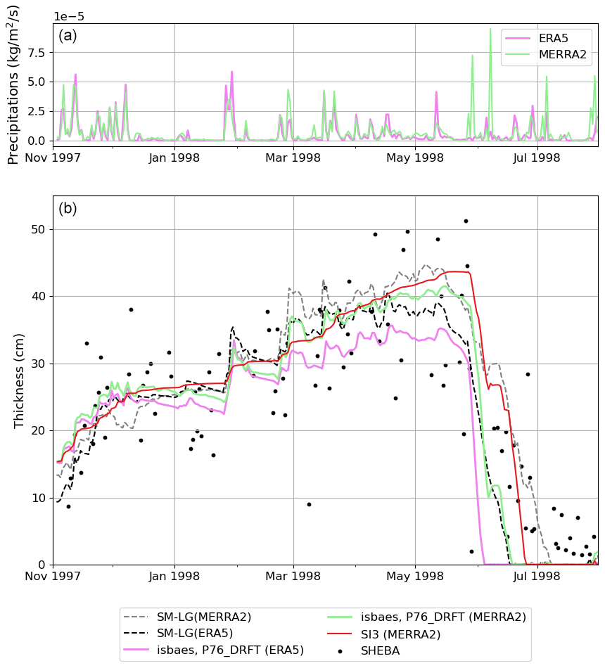
Figure 2 (a) Snow precipitation (in $\mathrm{kg}{\mathrm{m}}^{-\mathrm{3}}{\mathrm{s}}^{-\mathrm{1}}$) in MERRA-2 (green line) and ERA5 (magenta line) forcings. (b) Observed daily averages (black dots) and simulated (lines) snow thickness at the SHEBA tower during the November 1997–September 1998 period. The observations were aggregated over all transects (Perovich et al. 1999). The magenta line and the green line represent the snow thickness for a simulation using the P76_DRIFT configuration using ERA5 and MERRA-2 as forcing, respectively. The dashed lines represent the snow thickness from the SnowModel-LG product, in light gray for the MERRA-2 forcing and dark gray for ERA5.

Table 3 Averaged scores obtained for the snow thickness (cm) during the November 1997 to August 1998 period for the sensitivity tests on the atmospheric forcing.

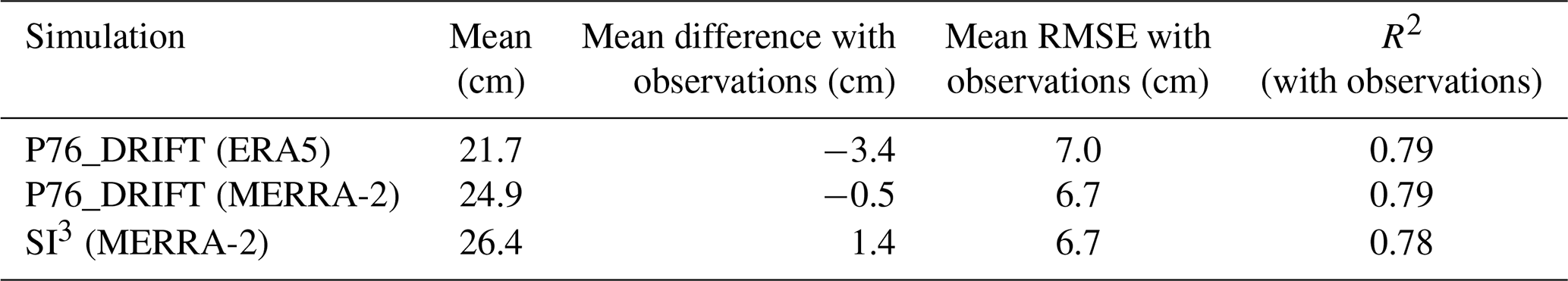
Overall, the snow thickness computed by ISBA-ES with the P76_DRIFT configuration compares well with the SHEBA observations and SnowModel-LG outputs (Fig. 2). When using ERA5 as the atmospheric forcing, snow thickness is slightly underestimated by an average of 3.4 cm over the period. In contrast, a better match with observations is achieved using MERRA-2, with the underestimation reduced to an average of 0.5 cm (refer to the scores in Table 3). In particular, the snowmelt is delayed in comparison to the ERA5 simulation because MERRA-2 reports more precipitation than ERA5 during the melt season (from May to August). During the SHEBA period, switching the atmospheric forcing from ERA5 to MERRA-2 results in an average change in snow thickness of approximately 3.2 cm in ISBA-ES simulations. This difference aligns with SnowModel-LG outputs, where the change in atmospheric forcing leads to an average change in snow thickness of around 3.1 cm.

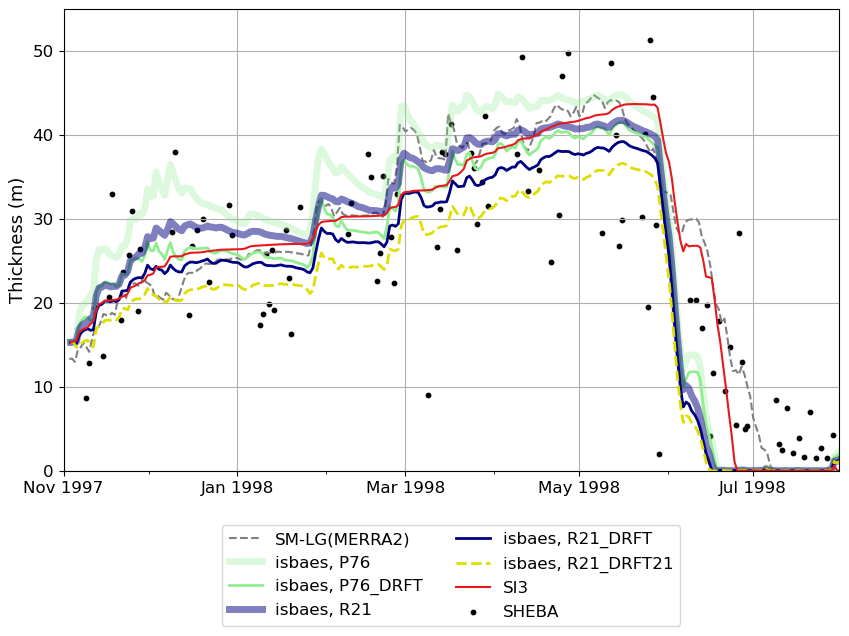
Figure 3 Observed daily averages (black dots) and simulated (lines) snow thickness at the SHEBA tower during the November 1997–September 1998 period. The observations were aggregated over all transects (Perovich et al. 1999). The thick green, thin green, thick blue, thin blue, yellow dashed, and red lines respectively show the P76, P76_DRFT, R21, R21_DRFT, R21_DRFT21, and SI³-only simulations, while the dashed gray line shows the SnowModel-LG data.

The mean differences of P76_DRIFT simulations with SnowModel-LG outputs are 2.2 cm for ERA5 simulations and 2.1 cm for MERRA-2. The temporal variability of SI³ + ISBA-ES simulations aligns more closely with the SnowModel-LG outputs compared to the SI³-only simulation, where the snow thickness varies less over time. This is because SI³ + ISBA-ES simulates the temporal evolution of precipitation density, making it more responsive to changes in atmospheric temperature and wind compared to the SI³-only simulation in which the density of the snowfall is constant.

3.1.2 Sensitivity to the parameterization of snowfall density and snowdrift

This section focuses on analyzing the effects of changing the parameterizations for snowfall density and wind-driven snow compaction (snowdrift). Given that better agreement with the observations was achieved using MERRA-2 as atmospheric forcing, we decided to use this forcing for our simulations. Therefore, the MERRA-2 reanalysis is used to force all simulations presented in the rest of the article.

We performed six simulations with the P76, P76_DRIFT, R21, R21_DRIFT, R21_DRIFT21, and SI³ configurations over the period and the path of the SHEBA experiment (Perovich et al., 1999) as described in the previous section.

Table 4 Averaged scores obtained for the snow thickness (cm) during the November 1997 to August 1998 period for the sensitivity tests on the snow density parameterizations.

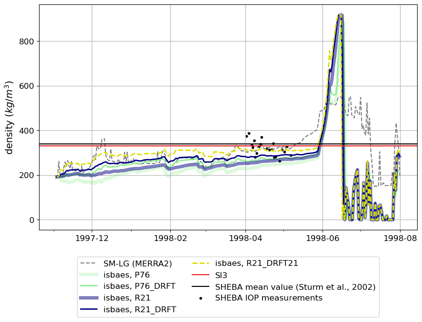
Figure 4 Snow density at the SHEBA tower during the November 1997–September 1998 period. The black dots represent the daily averages of the SHEBA density measurements made during the intensive observation period in April.

Figure 3 depicts the aggregated snow thickness from all SHEBA transects compared to our simulations and to SnowModel-LG outputs. The scores obtained for each simulation are summarized in Table 4. Overall, all simulations compare reasonably well with the measured snow thickness from SHEBA during the accumulation period. The best scores are nonetheless obtained for the P76_DRIFT simulation (see Table 4). As expected, the snowdrift parameterization tends to reduce the snow thickness through snow compaction by ∼ 3.9 cm (P76 – P76_DRIFT) on average over the period for the default parameters and by ∼ 5.1 cm with the Royer et al. (2021) parameters for the snowdrift and the snowfall density (R21 – R21_DRIFT21). The choice of the parameterization for the snowfall density and for the snowdrift results in an average change in snow thickness of approximately 3.9 cm in ISBA-ES simulations (P76_DRIFT – R21_DRIFT21), which is roughly the same order of magnitude as the thickness change associated with the choice of atmospheric forcing (see Sect. 3.1.1).

However, the snow tends to disappear in all simulations during the first month of the melting season, while it persists until the end of the melting season (roughly from May to August) in the observations. In the melt season (from May 1998), the excessively fast melting of the snow in all ISBA-ES simulations compared to the SHEBA observations and the SI³-only simulation is likely due to the ISBA-ES albedo parameterization, which seems to underestimate the albedo during the melt season. Indeed, when the snow albedo is forced to 0.8 (which is higher than the albedo simulated with ISBA-ES, see Fig. 9), the snow thickness gets closer to the SnowModel-LG simulation during the melt period (see Fig. S1 in the Supplement). This underestimation of the albedo is probably due to its dependency on the density. Indeed, the albedo depends on the snow specific area, which is affected by the snow metamorphism (which is not explicitly represented by ISBA-ES), rather than on the snow density (e.g., Xiong and Shi, 2018)

The SI³-only simulation reproduces the snowmelt more successfully, resulting in thicker snow during this period. The better performance of the SI³-only simulation during the melt season may be attributed to its use of a constant snow albedo (0.83, see Fig. 9).

Note that the snow melts completely in summer in all simulations (including SnowModel-LG simulations), whereas snow remains in the observations, which also shows that the snowmelt is likely to be overestimated by the models.

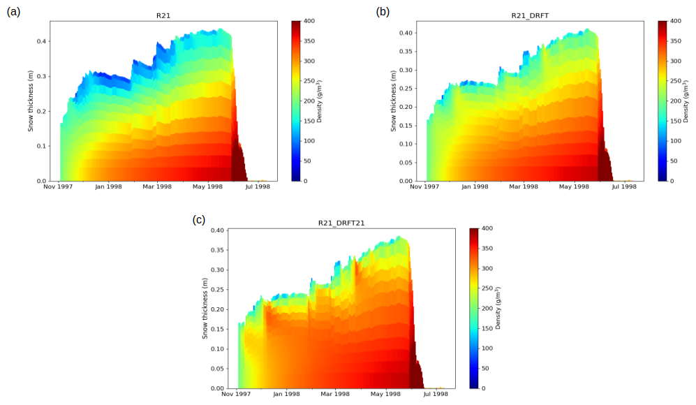
Figure 5 Snow thickness and density (contours) for R21 (a), R21_DRIFT (b), and R21_DRIFT21 (c) at the SHEBA tower during the November 1997–June 1998 period.

The first-order discrepancies in snow thickness between the different ISBA-ES simulations are related to the density of snow: since during compaction processes the mass remains constant, a denser snow will be associated with a thinner snowpack and vice versa. The evolution of the density during the SHEBA period is represented in Fig. 4. For the ISBA-ES simulations, the mean densities over this period are 225.6, 260.7, 244.6, 275.5, and 303.9 g m⁻³ for P76, P76_DRIFT, R21, R21_DRIFT, and R21_DRIFT21, respectively, which is slightly lower than the average bulk density of 340 g m⁻³ measured during SHEBA by Sturm et al. (2002) and with the mean densities of SnowModel_LG outputs (281.8 g m⁻³ when forced by MERRA-2 and 263.0 when forced by ERA5). Better agreement with the SnowModel-LG depth-averaged density is found for the ISBA-ES simulations using the snowdrift parameterization (P76_DRIFT and R21_DRIFT).

Over the Arctic region, the snowpack typically consists of a basal depth hoar (low-density, brittle, highly permeable type of snow) overlaid by a hard and dense wind slab (e.g., Domine et al., 2018; Sturm et al., 2002, and references therein). Without the snowdrift parameterization activated, the snowpack is not compacted near the surface (Fig. 5a). Consequently, the P76 (not shown, similar to R21) and R21 simulations fail to represent the typical Arctic wind slab layer. Alternatively, the default ISBA-ES snowdrift parameterization (Brun et al., 1997) tends to increase the near-surface density (Fig. 5b). However, the maximum density in the Brun et al. (1997) snowdrift parameterization is 350 g m⁻³, which is lower than the mean density of the wind slab layers found during SHEBA in Sturm et al. (2002) (403 g m⁻³). Therefore, the P76_DRIFT (not shown, similar to R21_DRFT) and R21_DRIFT simulations still lack an accurate representation of the wind slabs. In contrast, the Royer et al. (2021) snowdrift parameterization allows for higher densities and yields significantly different results (Fig. 5c). During winter, R21_DRIFT21 simulates higher densities near the snowpack surface, which could be attributed to a wind slab layer. Thus, although R21_DRIFT21 appears to overestimate the mean density, likely due to an inaccurate representation of the depth hoar layer, it does allow for a more realistic representation of wind slab layers in the Arctic region. In SI³, the density is constant and equal to 330 g m⁻³. The snow mass (not shown) remains unaffected by the choice of the parameterization for snowfall density and/or wind-induced compaction in the accumulation period. In the melt season, however, the melt rates are affected by the differences in heat diffusion associated with the differences in thermal conductivity, themselves dependent on the snow density.

Indeed, the snow density drives its thermal conductivity and thus the heat transfer within the snowpack. In SI³, it is a fixed parameter at 0.31 $\mathrm{W}{\mathrm{m}}^{-\mathrm{1}}{\mathrm{K}}^{-\mathrm{1}}$ (Vancoppenolle et al., 2023), which is the value measured during SHEBA by Sturm et al. (2002), but in ISBA-ES it can evolve as a function of the density. Figure 6 represents the time series of the snow thermal conductivity for SI³-only and SI³ +ISBAES simulations. The snowpack bulk conductivity from December 1997 to April 1998 is 0.10 $\mathrm{W}{\mathrm{m}}^{-\mathrm{1}}{\mathrm{K}}^{-\mathrm{1}}$ for the simulations without the snowdrift parameterization, 0.11 $\mathrm{W}{\mathrm{m}}^{-\mathrm{1}}{\mathrm{K}}^{-\mathrm{1}}$ for the simulations using the Brun et al. (1997) snowdrift parameterization, and 0.14 $\mathrm{W}{\mathrm{m}}^{-\mathrm{1}}{\mathrm{K}}^{-\mathrm{1}}$ with the Royer et al. (2021) snowdrift parameters. Those conductivity estimates are consistent with the measured bulk conductivity during SHEBA (0.14 $\mathrm{W}{\mathrm{m}}^{-\mathrm{1}}{\mathrm{K}}^{-\mathrm{1}}$, Sturm et al., 2002) but since the publication of the SHEBA datasets the conductivity measurements have been questioned and they are thought to be too low (Calonne et al., 2019; Riche and Schneebeli, 2013). Sturm et al. (2002) estimated a thermal conductivity of 0.31 $\mathrm{W}{\mathrm{m}}^{-\mathrm{1}}{\mathrm{K}}^{-\mathrm{1}}$, inferred from ice growth and temperature gradients. Thus, the thermal conductivity simulated by ISBA-ES might be slightly underestimated.

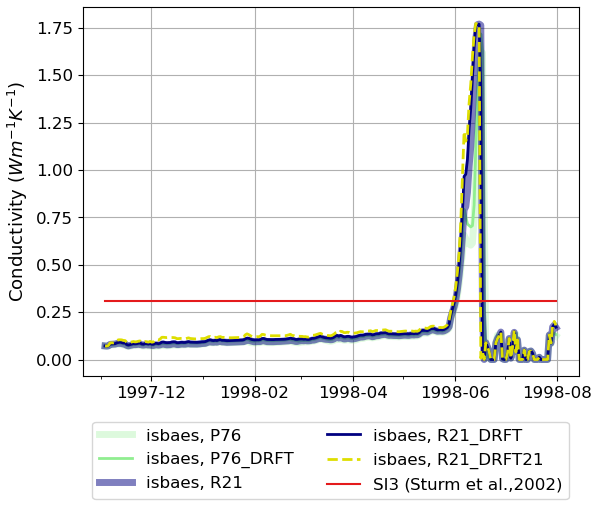
Figure 6 Snow conductivity at the SHEBA tower during the November 1997–September 1998 period.

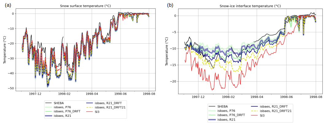
Figure 7 Measured and simulated snow surface (a) and snow–ice interface (b) temperatures (°C) at the SHEBA tower during the November 1997–September 1998 period. The black line shows the observations; the colored lines show the simulations as in Fig. 3.

The thermal conductivity drives the heat transfer through the snowpack. The snow surface temperature and the snow–ice interface temperature were measured at the SHEBA tower during the whole SHEBA period. Figure 7 represents the measured and simulated snow temperatures at both the snow surface and at the sea–ice interface. Note that the snow temperatures were not available in the SnowModel-LG outputs. The snow surface temperature is strongly dependent on the atmospheric forcing, and all SI³ + ISBA-ES or SI³-only simulations compare well with the observations and simulate a snow surface temperature consistent with the observations and a realistic temporal variability. The surface temperature simulated by ISBA-ES simulations is slightly too cold by between ∼ −3 and −4 °C compared to the observations, while the bias in the SI³-only simulation is about −2.4 °C on average over the accumulation and melt periods (from January to June 1998). All SI³ + ISBA-ES simulations simulate a snow–ice interfacial temperature more consistent with the observations than the SI³-only simulation, with a mean difference of 0.8 °C for P76 and −2.7 °C for R21_DRFT21 simulations, against −6 °C for SI³ on average over the accumulation and melt periods. Thus, this suggests that the thermal conductivity simulated by ISBA-ES is more realistic than the mean value used in SI³ (even though it seems slightly underestimated compared to the observations). The ISBA-ES model also simulates a more realistic bottom snow temperature in the melt season (from the end of May) compared to SI³. Note that the best agreement with the observations is found for the P76_DRIFT simulation. The lowest interfacial temperatures simulated by the SI³ + ISBA-ES range from ∼ −12 °C for P76 to ∼ −18 °C for R21_DRIFT21 simulations. Note that this range depends on the parameterization used for the computation of the snow thermal conductivity (i.e., Sturm et al., 1997, parameterization), as we found a bigger range of temperatures with the Anderson (1976) parameterization (used in the ISBA-ES default version) (not shown). In brief, these results highlight the sensitivity of the snowpack bottom temperature to the choice of the parameterization for the snowfall density and/or wind compaction through their impact on the snow density and ultimately the snow conductivity, but also the importance of simulating a realistic thermal conductivity in the snowpack as it will condition the sea ice growth and melt below.

In all ISBA-ES simulations, the thermal conductivity of snow is lower than the value prescribed in SI³. This results in a more insulating snow layer that reduces heat loss from the sea ice to the atmosphere, thereby keeping the ice warmer and thinner (Fig. 8). Consequently, all ISBA-ES simulations produce thinner sea ice compared to SI³, with mean sea ice thicknesses (averaged from November 1997 to August 1998) of 2.17, 2.21, 2.18, 2.22, and 2.26 m for the P76, P76_DRFT, R21, R21_DRFT, and R21_DRFT21 experiments, respectively, versus 2.36 m in SI³. While SI³ simulates a mean sea ice thickness closer to the observed value of 2.38 m during the same period, the onset of melting is delayed by approximately 15 d relative to the observations. In contrast, although the ISBA-ES simulations underestimate the sea ice thickness, they reproduce a melt onset timing that aligns well with the observations. The sensitivity of the sea ice thickness to the choice of the parameterization for the snowfall density and the snowdrift is around 6 cm on average over the SHEBA period (R21_DRFT21-P76_DRFT). However, since the sea ice thickness at the end of the melt season is different between the different simulations, we could expect this sensitivity to grow in longer simulations.

Figure 8 Measured and simulated sea ice thicknesses (m) at the SHEBA tower.

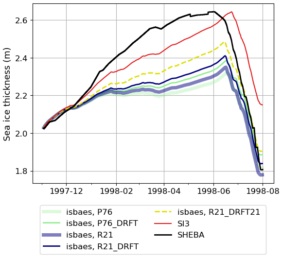
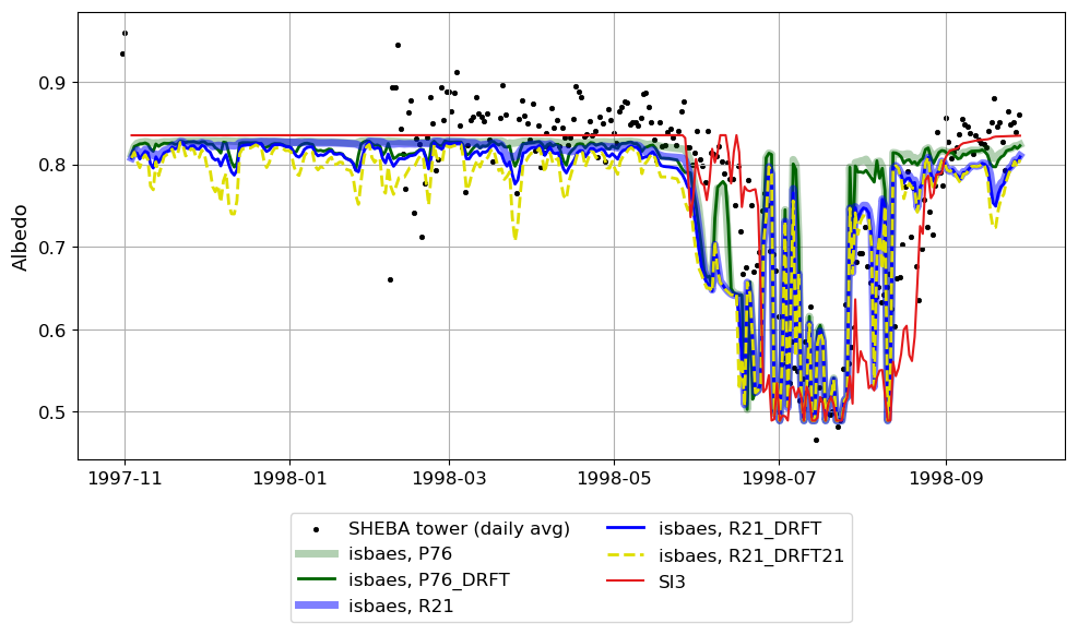
Figure 9 Daily averages of measured (dots) and simulated (lines) snow–ice albedo at the SHEBA tower during the November 1997–September 1998 period.

The snow/ice albedo was also measured at the SHEBA tower during the melt season, and it is represented in Fig. 9 along with the albedo simulated by SI³ + ISBA-ES and SI³-only simulations. In SI³, the snow albedo is fixed to 0.83 and it is constant during the accumulation period, which is roughly consistent with the observations at the SHEBA tower (Fig. 9). In SI³ + ISBA-ES simulations, the albedo varies with the snowpack density and thus it is sensitive to the choice of the parameterization for the snowfall density and/or wind compaction. It is slightly lower than the albedo in SI³ as it is bounded to 0.83 and decreases when the density increases. P76 and R21 simulate a realistic albedo, but the other simulations underestimate the albedo. When the snowdrift parameterization is active, the albedo fluctuates more as it depends on the density of the first layer, which is very sensitive to the compaction by wind.

4 Discussion and conclusion

Here we implemented for the first time a detailed snow-physics scheme (ISBA-ES) into a sea ice model (SI³), which serves as the sea ice component for upcoming versions of the CNRM-CM climate model. The ISBA-ES snow model incorporates detailed representations of snowpack properties such as density, grain size, and thermal conductivity, allowing for more accurate simulation of snow accumulation, compaction, metamorphism, and melt processes than usual slab models (such as the original snow parameterization in SI³ that uses a constant density and thermal conductivity). Its integration into SI³ does not use a coupler and the ISBA-ES code is compiled within the SI³ framework.

The integration of such a detailed snow model within a sea ice model is, per se, a technical challenge. We integrated ISBA-ES to SI³ so that snow thermodynamic processes are not computed anymore by SI³ but by ISBA-ES. However, we aimed at modifying as little as possible the ISBA-ES model to facilitate the phasing with the future versions of the model. Thus, some sea-ice-related processes (thus not resolved by this alpine snow model) such as the snow–ice formation are still resolved within the sea ice model. At the snow–ice interface, transfer of heat from snow to ice is made through a heat conduction flux. The SI³ + ISBA-ES model is currently fully functional in 1D without the sea ice dynamics activated and conserves the heat, mass, and salt.

The aim of this article was to present the first developments made to allow the integration of ISBA-ES into SI³ and the performance of the model, focusing on the thermodynamic processes only. Here, we validated the SI³ + ISBA-ES model over 1D configurations following the path of the Heat Budget of the Arctic Ocean (SHEBA) experiment (Perovich et al., 1999). We performed several simulations using different parameterizations for computing the snowfall density and the compaction by wind to illustrate the sensitivity of our model to these parameterizations. We compared these simulations with the SHEBA observations and with the SnowModel-LG outputs from Stroeve et al. (2020), which is, to date, the most sophisticated and validated snow-on-sea ice model available. Overall, our model simulates realistic snow thicknesses, densities, and temperatures compared to the SHEBA observations and SnowModel-LG outputs and captures the temporal variability of these variables well. Compared to the previous snow scheme used in SI³ that assumes constant snow density and thermal conductivity, our model is able to realistically simulate the temporal evolution of the snow bulk density and thermal conductivity of the snowpack. As a result, the temperature at the snow–ice interface is more accurate with SI³ +ISBAES compared to the previous SI³ snow scheme, leading to a more realistic heat transfer to the underlying sea ice and more realistic sea ice upper temperatures. This emphasizes the importance of modeling the temporal changes in the density and thermal conductivity of the snow layers on Arctic sea ice. In ISBA-ES, the sea ice is more insulated from the atmosphere than in SI³ due to the lower thermal conductivity of snow, which results in warmer and thinner ice. Consequently, the SI³-only simulation yields a mean sea ice thickness closer to observations, whereas ISBA-ES appears to better capture the timing of the melt onset. This underestimation of sea ice thickness in the SI³ + ISBA-ES simulations may result from several factors: (1) the one-dimensional nature of the simulation, which excludes dynamical processes; (2) the absence of certain physical processes, such as the formation of superimposed ice and the diffusion of water vapor through snow, that can influence sea ice growth; and (3) the SI³ sea ice model being tuned for snow with higher thermal conductivity. Nonetheless, the results show a physically consistent response of sea ice thickness and demonstrate a realistic coupling between snow and sea ice.

In agreement with Lecomte et al. (2013), we demonstrated that snowpack thicknesses, densities, and thermal conductivities are equally sensitive to the parameterization choices for computing snowfall density and representing snow compaction by wind, as well as to the choice of atmospheric forcing. Therefore, specific tuning of these ISBA-ES parameterizations is as crucial as having realistic forcing to accurately represent the snowpack over the Arctic. The best agreement with the SHEBA observations for snow thickness and temperature is achieved using the Brun et al. (1997) parameters for snowfall density and snow compaction (the default parameters of ISBA-ES). However, given (1) the significant spatial variability of Arctic snow cover, (2) the resolution disparity between model grid cell area estimates and point measurements during SHEBA, and (3) the uncertainties in observations, it is difficult to highlight the superiority of any SI³ + ISBA-ES configuration over another. Nonetheless, our results highlight the realism of the SI³ + ISBA-ES model and the importance of the choice of such parameterizations.

However, our study highlights the limitations of the current version of the SI³ + ISBA-ES model. While the model produces realistic depth-averaged densities, the vertical density profiles it simulates are not accurate. The model fails to accurately represent the typical Arctic snowpack, which generally features a basal depth hoar layer beneath a hard, dense wind slab. This inaccurate representation of the density profiles suggests that certain polar-specific processes may be missing from the model. For instance, incorporating a representation of water vapor fluxes within the snowpack could benefit the model. Indeed, the strong temperature gradients in the Arctic snowpack create gradients in saturation water vapor density and pressure, which result in diffusion (Sturm and Benson, 1997) that can significantly influence the snowpack's density profiles (Domine et al., 2016; Jafari and Lehning, 2023). In addition, we also demonstrated that the default maximum density according to Brun et al. (1997) for the snowdrift parameterization is insufficient for accurately capturing the upper wind slab layer typical of the Arctic region. Setting a higher maximum density as proposed by Royer et al. (2021) appears to better represent this wind slab layer, although it results in a slightly overly dense snowpack. However, the absence of long-term records of snow density profiles over sea ice complicates the tuning of wind compaction parameterizations. Future field studies collecting such data could significantly enhance the fidelity of density profiles in Arctic snow models. The model also seems to overestimate the albedo decrease during the melt season, leading to a rapid snowmelt. This underestimation is possibly due to a misrepresentation of the surface scattering layer in our model that was observed in the melt season during SHEBA (Perovich, 2005).

The model could also be further improved by incorporating specific snow-on-sea ice processes that are not yet represented in SI³ + ISBA-ES, such as the formation of superimposed ice, or by incorporating more recent parameterizations of the thermal conductivity (e.g., Macfarlane et al., 2023). Thus, despite the current limitations of the model, the implementation of such an intermediate-complexity snow model within the SI³ framework will facilitate further developments (in particular, the inclusion of polar-specific snow processes) that were not achievable with the previous, overly simplistic bulk snow model of SI³.

Since this study focuses solely on the thermodynamics of snow and sea ice, it serves as a preliminary step towards the full integration of ISBA-ES within SI³ and, subsequently, the CNRM-CM framework. The complete integration of ISBA-ES within SI³ requires the implementation of advection for time-varying snow layers, which is currently in progress. The next version of the model will be capable of simulating the spatial and temporal evolution of the snowpack on both level and deformed ice, thanks to the use of multiple sea ice categories and the incorporation of a subgrid-scale distribution of snow thicknesses.

Following this, SI³ + ISBA-ES must be coupled with the atmosphere to achieve its full integration within the CNRM-CM framework. This will require additional development to enable the snow model to be driven by atmospheric heat fluxes. In the current code version, these fluxes over snow are calculated within the ISBA-ES model, which is appropriate for a forced mode but not feasible within the existing CNRM-CM coupling approach, where surface heat fluxes are typically calculated in the atmospheric model. To conclude, this paper marks the starting point of developments towards an improved snow over sea ice in the CNRM-CM model.