A close look at using national ground stations for the statistical modeling of NO₂

Air pollution leads to various health and societal issues. Modeling and predicting air pollution over space have important implications in health studies, urban planning, and policy-making. Many statistical models have been developed to understand the relationships between geospatial data and air pollution sources. An important aspect often neglected is spatial heterogeneity; however, the relationships between geographically distributed variables and air pollutants commonly vary over space. This study aims to evaluate and compare various spatial and non-spatial statistical modeling (including machine learning) methods within different spatial groups. The spatial groups are defined by traffic- and population-related variables. Models are classified into local and global models. Local models use air pollution measurements from the Amsterdam area. Global models use ground station observations in Germany and in the Netherlands. We found that prediction accuracy differs substantially in different spatial groups. Predictions for places near roads with high populations show poor prediction accuracy, while prediction accuracy increases in low-population-density areas for both local and global models. The prediction accuracy is further increased in places far from roads for global models. Modeling of air pollution in different spatial groups shows that nonlinear methods can have higher prediction accuracy than linear methods. The spatial prediction patterns of global models show that nonlinear methods generally are less sensitive to extreme values compared to linear methods. Additionally, clusters of predicted air pollution differ between models within cities despite similar prediction accuracy. Also, the influence of predictors on NO₂ concentrations varies across different cities. Using the local dataset of our study and explicitly accounting for spatial autocorrelation in the universal and ordinary kriging models does not improve accuracy; however, analyzing prediction performance across spatial groups provides valuable insights. Comparing local and global prediction patterns reveals that local models capture regional clusters of high air pollution, which are not detected by global models. These findings highlight the fact that solely relying on overall prediction accuracy can be insufficient and potentially misleading, underscoring the importance of considering spatial variability and model performance within different spatial groups.

1 Introduction

Modeling and estimating NO₂ concentration levels are essential for a comprehensive understanding of air pollution, which plays a critical role in urban planning and policy-making to promote public health. Air pollutants have been modeled across various spatial scales, from local to global. These models can be broadly classified into three categories: statistical models, chemical transport models, and air dispersion models. Chemical transport models are typically used for large-scale air pollution modeling, while air dispersion models require detailed, spatially resolved emission lists to capture small-scale variations in pollutants (Beelen et al., 2013).

In recent years, statistical modeling has gained popularity for high-resolution mapping at different spatial scales, driven by the increasing availability of predictors (e.g., GIS variables) and advancements in computational capabilities. Land use regression (LUR) is the most well-known statistical approach for air pollution modeling, employing linear regression to capture the spatial variability in traffic-related air pollution in urban areas. Most LUR models rely on data from ground monitoring stations (Hoek et al., 2008; Wang et al., 2020). Geostatistical methods like kriging can further account for spatial correlations between observations. However, several studies have favored the simplicity of LUR, often concluding that it performs as well as or better than geostatistical methods (Hoek et al., 2008; Marshall et al., 2008; Beelen et al., 2013). Notably, these conclusions are typically based solely on prediction accuracy, without considering the models' ability to quantify uncertainty, offer scientific interpretation, or integrate known physical mechanisms (Lu et al., 2023). Specifically, many studies neglect the optimal estimation of the covariance function and the specification of priors in geostatistical modeling.

Although linear regression models are advantageous for their interpretability and ability to extrapolate, they may not capture the complex processes of air emission, dispersion, and deposition (Wang et al., 2020). As a result, data-driven nonparametric models, commonly referred to as machine learning methods in air pollution mapping, have become increasingly popular. These models, such as ensemble tree-based algorithms, are better suited for capturing the nonlinear relationships between pollutants and predictors (Weichenthal et al., 2016; Reid et al., 2015; Lu et al., 2020). For instance, Brokamp et al. (2017) compared land use random forest (LURF) models with LUR models to measure elemental components of PM_2.5 in Cincinnati, Ohio, and found that LURF models had lower prediction error variance across all elemental models when cross-validated. Similarly, Kerckhoffs et al. (2019) reported that machine learning algorithms, such as bagging and random forests, explained more variability in ultra-fine particle concentrations than multiple-linear-regression and regularized-regression techniques. Ameer et al. (2019) advocated for random forest regression as the best technique for pollution prediction in varying datasets, locations, and characteristics, as it outperformed decision tree regression, multilayer perceptron regression, and gradient boosting regression. Ren et al. (2020) also concluded that nonlinear machine learning methods achieve higher accuracy than linear LUR, emphasizing the importance of careful hyperparameter tuning and robust data splitting and validation to ensure stable, reliable results. Chen et al. (2019) compared 16 algorithms for predicting annual average fine-particle (PM_2.5) and nitrogen dioxide (NO₂) concentrations across Europe. They found that ensemble-tree-based methods were particularly effective for PM_2.5, while NO₂ models showed similar R² values across different methods. Importantly, they reported a high correlation between the predicted values of various models, noting that the most influential predictors differed substantially between pollutants. For example, satellite observations and dispersion model estimates were key predictors for PM_2.5 concentrations, while NO₂ variability was primarily driven by traffic-related variables. The significant contribution of road traffic to NO₂ levels is further supported by Wong et al. (2021), whose modeling results implied that nitrogen emissions are influenced by long-range transport from gasoline-fueled passenger cars in particular.

In recent years, the use of statistical modeling for air pollution mapping has surged, and models are increasingly applied to urban and geo-health studies. However, evaluating these models and maps remains challenging. One challenge is the scarcity of air pollution measurements. Another is the neglect of spatial heterogeneity in air pollution mapping. For example, He et al. (2022) acknowledge spatial heterogeneity in measurement stations by demonstrating that the probability density functions of concentrations (NO, NO₂, PM₁₀, PM_2.5) vary across different spatial categories (e.g., urban traffic, suburban/rural traffic, urban industrial, suburban/rural industrial, urban background, suburban background, rural background). However, their study does not model potential differences in the prediction accuracy across these categories. Most current statistical approaches assess only overall accuracy (Hoek et al., 2008; Chen et al., 2019). Hoek et al. (2008) reported that LUR models typically explain 60 %–70 % of the variation in NO₂, but this explained variation could be significantly lower near traffic. Chen et al. (2019) argued that many air pollution exposure studies fail to account for the characteristics of monitoring sites when performing cross-validation, potentially misrepresenting model results. They suggest evaluating models using pollution data from monitoring sites that reflect the application locations (Chen et al., 2019).

Finally, a consistent and coherent method for quantifying uncertainty in air pollution mapping is still lacking. As noted by Shaddick et al. (2020), uncertainty in air pollutant measurements is rarely discussed. This lack of evaluation can lead to overlooked biases, in particular because nonparametric machine learning methods often lack extrapolation capabilities. When prediction areas differ significantly from the training data in their societal and environmental characteristics, this can result in highly biased estimates that are rarely examined in many studies (Shaddick et al., 2020).

Given the growing number of modeling and prediction techniques and the risk of misrepresenting spatial patterns due to data heterogeneity, this study seeks to answer the following research questions:

1. To what extent can statistical models predict NO₂ concentrations using high-quality, high-temporal-resolution ground station measurements?

2. How do the performance and spatial accuracy of these models vary?

This study focuses on the Netherlands and Germany and uses two datasets: the official national ground station measurements from both countries (referred to as the global dataset) (OpenAQ, 2017; EEA, 2021) and the more dense long-term measurements collected by Palmes tubes in Amsterdam from the Amsterdam area (referred to as the local dataset) (Gemeente Amsterdam, 2022). Palmes tubes are passive samplers used in the routine monitoring network that measure NO₂ on street lanterns and building facades in Amsterdam. The global dataset includes 482 measurement stations covering 398 000 km² (0.0012 points km⁻²), while the local dataset contains 132 stations across 196 km² (0.591 points km⁻²). The study aims to compare and understand model behaviors and prediction patterns across (1) the two datasets, (2) different spatial groups classified by proximity to traffic and population density, and (3) various statistical models to evaluate the added value of nonlinear machine learning models and geostatistical approaches.

2 Methodology

2.1 Data

The global and local datasets include the annual mean NO₂ concentrations (measured in µg m⁻³) for the year 2017 (OpenAQ, 2017; EEA, 2021). Figure 1 presents the distribution of NO₂ concentrations at the global and local measurement stations. The terms “global” and “local” were chosen to reflect the relative scale of the datasets, with “global” representing a broader, cross-national dataset and “local” focusing specifically on Amsterdam. While the “global” dataset includes only two neighboring countries, this terminology emphasizes its wider scope compared to the local dataset. The global dataset comprises ground station measurements from Germany and the Netherlands, while the local dataset includes the Palmes data in the Amsterdam region.

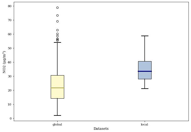
Figure 1 Distribution of NO₂ concentrations in the global (yellow) and local (blue) datasets.

The spatial distribution of NO₂ measurement stations is provided in the Supplement (Figs. S1 and S2). Urban areas generally have a higher density of measurement stations. This study focuses on the differences between global and local models, particularly in Amsterdam, while also considering the city's less densely populated areas to examine the urban impact on predicted NO₂ concentrations in the local models.

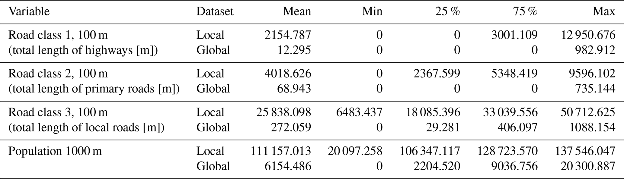
To evaluate whether prediction quality varies across areas with different characteristics of spatial patterns (e.g., high vs. low road density), the global and local datasets are divided into three spatial groups based on population density and traffic-oriented variables. Population data for 2015 from the Global Human Settlement Layer are used (JRC, 2015), and road length information is sourced from OpenStreetMap (2019). Descriptive statistics for the variables used to define the spatial groups are presented in Table 1.

Table 1 Descriptive statistics of variables determining the spatial groups for the local and global datasets. The statistics are derived from the station measurement locations. The distances in the “variable” column represent different buffer radii around measurement stations.

The three spatial groups are defined as follows:

1. Urban. Areas within 100 m of road class 1 (highways) or 2 (primary roads) and with a population density in the highest 25 % or areas where both road class 3 (local roads) values and population density are in the highest 25 %.

2. Suburban. Areas within 100 m of road class 1 or 2 with a population density in the lowest 75 % or areas where road class 3 values are in the highest 25 % and population density is in the lowest 75 %.

3. Rural. Areas further than 100 m from road class 1 or 2 or areas where road class 3 values are in the lowest 75 %.

This classification resulted in 85 observations being labeled as “urban”, 138 as “suburban”, and 259 as “rural”, totaling 482 observations in the global dataset. Given the smaller sample size of the local dataset, the threshold for defining “urban” was adjusted from the 75th percentile to the 50th percentile, which had a converging effect on the relative group sizes. Moreover, the increase in samples classified as “urban” is desirable, as this group exhibits relatively high heterogeneity. The local dataset consists of 56 observations classified as “urban”, 46 as “suburban”, and 30 as “rural.”

Although this adjustment introduces some inconsistency between the global and local definitions of “urban”, it addresses the challenge of unequal distributions of instances across groups in the local dataset, which could introduce bias into the statistical learning models. The threshold adjustment represents an initial step toward mitigating such effects by ensuring a more balanced representation of spatial characteristics within the local model. Figures S3 and S4 show the spatial distribution of observations among these groups for both datasets, while Figs. S5 and S6 show the measured NO₂ concentrations per station.

Spatial predictors

We utilized a set of variables derived from Lu et al. (2020), including data on industrial areas, road lengths, population density, Earth night lights, wind speed, temperature, elevation, TROPOMI level 3 NO₂, and global radiation. A complete list of these variables is available in the Supplement (Table S1). Precipitation data were sourced from weather stations (National Centers for Environmental Information, 2017) and interpolated using ordinary kriging to cover the NO₂ measurement stations. Kriging parameters are detailed in the Supplement (Sect. S2.4, “Parameters”).

Building density was obtained from the World Settlement Layer 2015 dataset available on Figshare (Marconcini et al., 2020). In line with previous studies (Beelen et al., 2013; Kheirbek et al., 2014), we considered various buffer sizes (100, 500, 1000 m) around measurement stations to account for spatial proximity effects, especially in densely populated urban areas. Normalized difference vegetation index (NDVI) values were obtained from NASA (NASA, 2017).

Traffic volume data were sourced from the Nationaal Dataportaal Wegverkeer (NDW) in the Netherlands (Rijkswaterstaat, 2017) and from the Bundesanstalt für Strassenwesen (BAST) in Germany (Bundesanstalt für Strassenwesen, 2017). These data, generated by automatic counting stations, are expressed as average hourly traffic in 2017, with buffer sizes of 25, 50, 100, 400, and 800 m. The formula for calculating average hourly traffic is provided in the Supplement (Eq. S1).

2.2 Modeling NO₂ globally and locally

2.2.1 Ensemble trees

The global models use two types of statistical learning methods. The first group consists of ensemble-tree-based approaches, including the random forest and extreme gradient boosting (XGBoost). Hyperparameters are tuned based on cross-validation error. For the random forest model, the number of estimators is set to 1000, with a minimum sample split of 10, minimum samples per leaf of 5, maximum features per tree of 4, and a maximum depth of 10. The XGBoost model uses 10 000 estimators, with a reg_alpha of 2, reg_lambda of 0, max_depth of 5, and a learning rate of 0.0005 (see also Figs. S7 and S8). Additionally, the gamma for the XGBoost model is set to 5. Further details can be found in the Supplement (Sect. S1.1, “Parameters”, and Eq. S2; Boersma, 2025a). Additionally, the light gradient boosting (LightGBM) model was tested but did not yield significantly different results compared to XGBoost. The results of LightGBM analyses are shown in Figs. S9–S12.

2.2.2 Multiple linear regression

Key variables identified by the random forest model are used as predictors in multiple linear regression (MLR). The least absolute shrinkage and selection operator (LASSO) and ridge regularizations are employed to prevent overfitting. LASSO differs from ridge in that it uses the sum of the absolute values of the coefficients as a penalty, allowing some coefficients to be exactly zero and thus enabling feature selection (Ren et al., 2020). The alpha for both the LASSO and ridge models is tuned to 0.1 and is optimized using the lowest mean absolute error (MAE), root-mean-square error (RMSE), and highest R². The search grid ranges from 0.1 to 1 in increments of 0.1. Detailed parameters and mathematical formulations for linear regression, error terms, ridge regression, and LASSO regression are given in the Supplement (Sect. S1.2, “Parameters”, and Eq. S3; Boersma, 2025a).

2.2.3 Mixed-effects model and kriging

The performance of the random forest, XGBoost (Table S2), LASSO, and ridge models (Table S3) are unsatisfactory for the local dataset. Spatial modeling approaches including mixed-effects modeling and kriging are applied.

Mixed-effects models were able to capture hierarchical or grouped structures. In our study, the fixed effects correspond to the most influential predictors, such as population density, road length, and other traffic-related variables, which are assumed to have consistent effects across the entire study region. The random effects capture the spatial trends specific to different geographic regions, such as urban, suburban, and rural areas. For instance, local topography, vegetation, or specific traffic patterns in a region can create unique spatial trends. These spatial groups represent the variations in NO₂ concentrations due to local environmental factors and are modeled as random effects, allowing the model to account for spatial autocorrelation within regions.

This modeling approach is suitable because the spatial distribution of pollutants such as NO₂ is not random and tends to show clusters or gradients in traffic, land use, and population density. By modeling the spatial context as random effects, we capture these spatial dependencies and potentially improve the accuracy of predictions in different areas (Mullen and Birkeland, 2008; Lee et al., 2020).

Kriging is essentially a form of Gaussian process regression, developed and applied in geosciences with a focus on spatial prediction. It typically uses spatial coordinates as covariates and places a strong emphasis on variogram modeling to capture spatial dependence. The residuals of a linear regression model are treated as realizations of a spatial stochastic process, and their covariance is modeled to make predictions. Kriging is particularly suitable for estimating NO₂ concentrations, as NO₂ tends to vary smoothly over space.

In this study, ordinary and universal kriging are applied. Ordinary kriging assumes that the mean of the variable predicted is constant but unknown. It assumes stationarity without trend removal. Universal kriging assumes that the variable being predicted has a deterministic trend (e.g., linear or polynomial). The automap package in R (Hiemstra et al., 2009) is used to initialize the covariance parameters and to perform the kriging interpolation. Two separate models are created, one that incorporates the spatial groups (urban, suburban, rural) and one that does not. These models help to compare the effect of modeling spatial correlation on the prediction accuracy (Idir et al., 2021; Khan et al., 2023).

In total, 10 models are fit and compared: 4 using the global dataset and 6 using the local dataset, enabling a comprehensive evaluation of model performance across different geographical scales. The equations for kriging and the linear model are provided in the Supplement under the “Parameters” (S2.1–S2.3) and “Equations” (S4 and S5) sections.

2.3 Feature selection

Feature selection for global models is initially based on Shapley values (Shapley, 1953). While the variance inflation factor (VIF) is effective at detecting multicollinearity, it does not consider feature importance or interactions. The VIF results are available in Tables S4 and S5. Feature selection aims to remove irrelevant or highly correlated predictors that could generate unstable estimates and affect model interpretation (Araki et al., 2018).

Shapley values are calculated for each feature (i.e., predictor) based on its contribution ϕ_j to the prediction of NO₂ concentration levels compared to the average prediction across the dataset (Shapley, 1953). The contribution of a feature is determined by comparing the difference in the response variable when the feature is present vs. when it is absent (i.e., marginal contribution) (Algaba et al., 2019; Shapley, 1953). The formula for calculating Shapley values can be found in the Supplement (Eq. S6).

In this study, feature selection is guided by the out-of-sample performance in a random sampling validation repeated 10 times, where Shapley values are calculated for each iteration of the random forest models. Predictors are ranked based on the median Shapley value across all iterations. The relative positions of each predictor using the median-based approach are illustrated in Figs. S13 and S14, with the Shapley ranking of a single run shown in Fig. 2. The most influential predictors for the global models include nightlight intensity (450 and 3150 m buffers), population density (1000 and 3000 m buffers), road class (class 2 within 25 m and class 3 within 300 and 3000 m buffers), the annual mean NO₂ column density of 2018 measured by the TROPOMI instrument on board Sentinel-5p (trop mean filter 2018), building density in the 100 m buffer, NDVI, and traffic buffers (25 and 50 m buffers). Descriptive statistics of the most influential predictors for the global models are in Table 2.

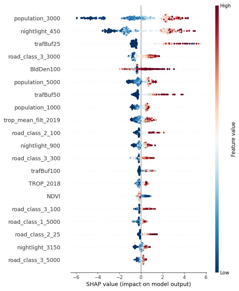
Figure 2 Variable importance ranked by Shapley values in a single run using the global dataset.

Table 2 Descriptive statistics for global predictors. bldden100 = built area within a 100 m buffer, NDVI = normalized difference vegetation index, nightlight_3150 = nightlight in a 3150 m buffer, nightlight_450 = nightlight in a 450 m buffer, population_1000 = population in a 1 km grid, population_3000 = population in a 3 km grid, road_class_2_25 = total length of primary roads in a 25 m buffer, road_class_3_300 = total length of local roads in a 300 m buffer, road_class_3_3000 = total length of local roads in a 3000 m buffer, trafbuf25 = traffic count in a 25 m buffer, trafbuf50 = traffic count in a 50 m buffer, trop_mean_filt_2018 = TROPOMI 2018 mean vertical column density. Note that the NDVI has a scale factor of 0.0001.

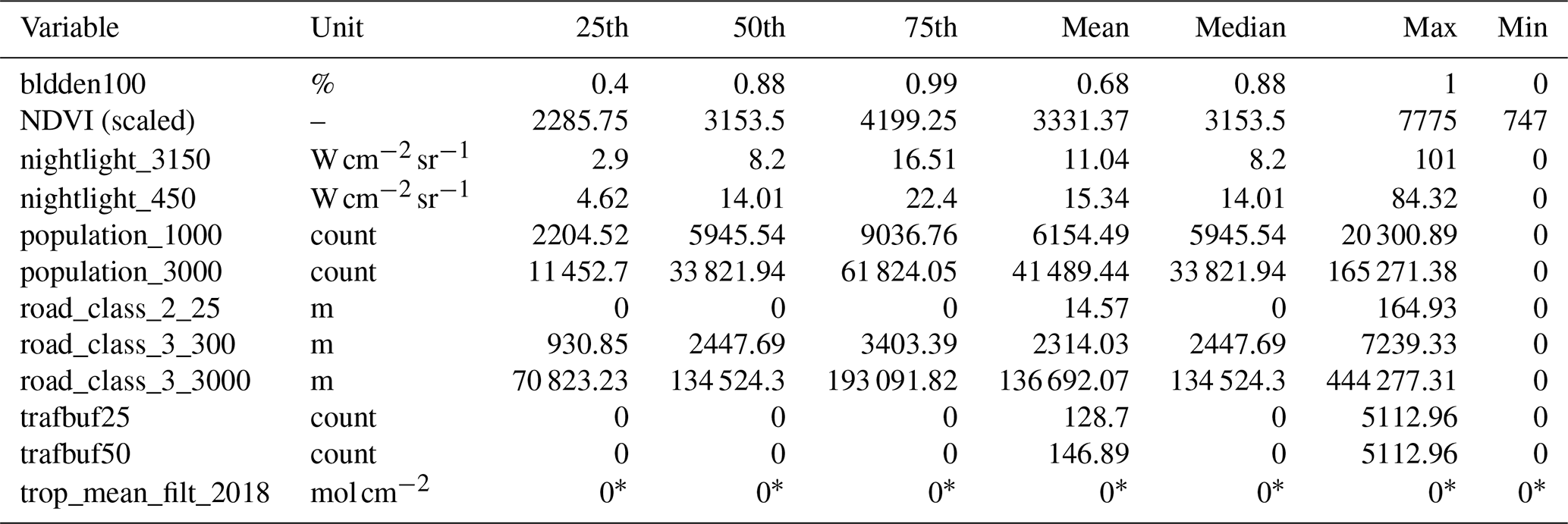
^* The values for trop mean filt 2018 are very small, on the order of 10⁻⁵.

A random forest algorithm is applied iteratively to determine the optimal number of predictors, starting with the 2 most influential predictors and extending to the 30 most influential features. The RMSE and R² metrics are used to evaluate the optimal number of predictors. The number of predictor variables and their corresponding evaluation scores (R², RMSE) are shown in Fig. 3. In particular, prediction accuracy improves significantly when considering at least 12 predictors, but the improvement is marginal beyond this number.

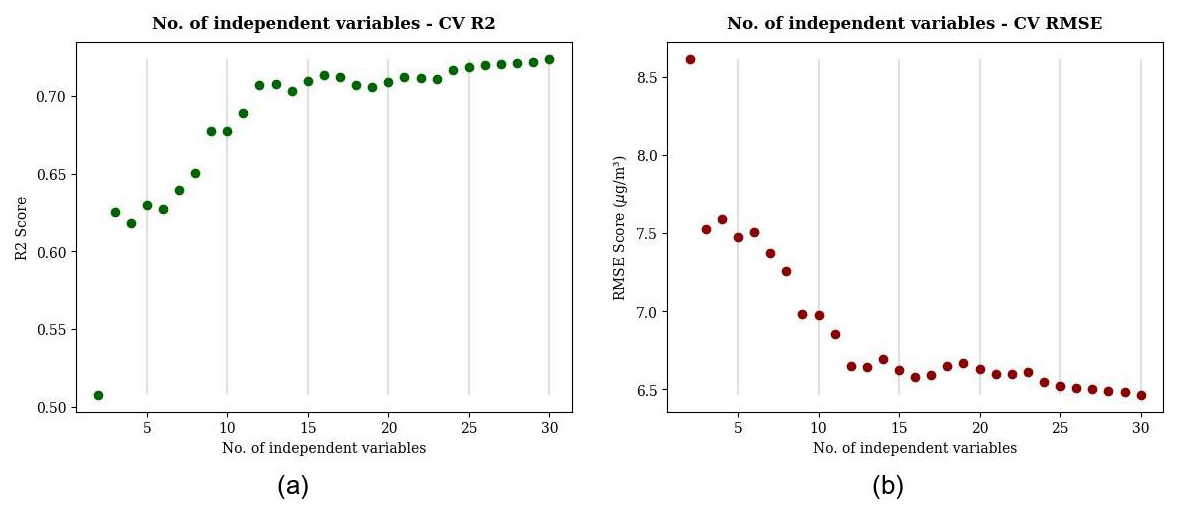
Figure 3 Out-of-sample performance in a random sampling validation repeated 10 times: the number of features and model performance based on the global dataset. The metrics shown include R² (a) and RMSE (b).

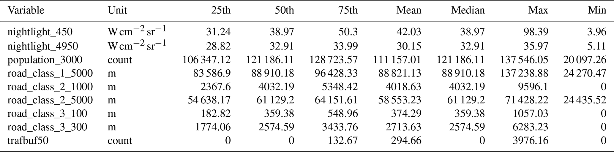
Due to the random forest model's poor performance across all local station measurements (Figs. S15–S17) and per spatial group (Table S2), the random forest algorithm is deemed unsuitable for identifying the number of variables for the local models. Instead, the best-subset regression is used for variable selection in local models. This approach tests all possible combinations of predictor variables (Kassambara, 2018), with a maximum of 30 predictors considered. The statistical criteria include adjusted R²; Mallows criterion p – with p referring to the number of predictors in the regression model; and Bayesian information criteria (BIC) scores. As a result, nine features are identified for the local models. The most influential predictors for the local models include nightlight intensity (450 and 4950 m buffer), population density (3000 m buffer), road class (class 1 within a 5000 m buffer, class 2 within 1000 and 5000 m buffers, class 3 within 100 and 300 m buffers), and the traffic buffer (50 m buffer). Descriptive statistics of the most influential predictors for the local models are in Table 3.

Table 3 Descriptive statistics for local predictors. nightlight_450 = nightlight in a 450 m buffer, nightlight_4950 = nightlight in a 4950 m buffer, population_3000 = population in a 3 km grid, road_class_1_5000 = total length of highway in a 5000 m buffer, road_class_2_1000 = total length of primary roads in a 1000 m buffer, road_class_2_5000 = total length of primary roads in a 5000 m buffer, road_class_3_100 = total length of local roads 100 m buffer, road_class_3_300 = total length of local roads in a 300 m buffer, trafbuf50 = traffic count in a 50 m buffer.

2.4 Model comparison

In global modeling, comparisons are made among tree-based models, random forest and XGBoost, and linear models, with LASSO and ridge penalization (the models are also called LASSO and ridge). For local modeling, we compare linear models, mixed-effect models, and kriging models. Each model is evaluated based on the standard matrix of R², RMSE, and MAE (Rybarczyk and Zalakeviciute, 2018; Ameer et al., 2019; Chang et al., 2020). For model evaluation, leave-one-out cross-validation (LOOCV) is employed for local models, while a random $\mathrm{90}/\mathrm{10}$ training–testing split is used for global models. Additionally, the prediction patterns of the local and global models are analyzed. To benchmark the model performance, a mobile NO₂ map of the study area (Kerckhoffs et al., 2019; Yuan et al., 2023) is used for comparison. This map provides detailed spatial information collected by two Google Street View cars that continuously measured NO₂ at a frequency of 1 Hz in Amsterdam from 25 May 2019 to 15 March 2020 (stopped due to the COVID-19 lockdown policy). We acknowledge that the temporal resolution of these benchmark data differs from the coarser temporal scales used in our models. The data used in Kerckhoffs et al. (2019) are over specific, limited time periods, while our models address predictions over broader temporal spans. Despite this temporal inconsistency, the detailed spatial granularity of the annual map from Kerckhoffs et al. (2019) provides valuable insights and remains an appropriate standard for assessing spatial prediction quality.

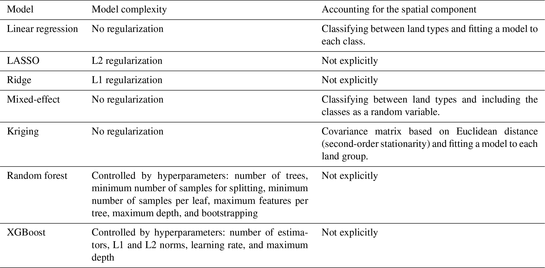
Table 4 provides an overview of the global and local models, along with selected predictors and evaluation methods. The global models are applied to areas with varying demographic characteristics, including two large cities with populations exceeding 700 000 (Amsterdam and Hamburg), a mid-sized city with around 350 000 inhabitants (Utrecht), and a small city with approximately 70 000 inhabitants (Bayreuth). The resolution of the analysis is 100 m, with raster files of the most important predictors resampled and converted into 100 m grid cells for these regions using spatial extraction methods. The influential predictor information (for global models, see Tables 2 and 4; for local models, see Tables 3 and 4) is recalculated at a 100 m resolution for the extent of the aforementioned regions. The 100 m by 100 m grid cells containing predictor information are used to predict NO₂ values for the respective 100 m grids based on the trained local and global models (Lu et al., 2020, 2023). The 100 m grid resolution is consistently applied in the predictions for both local and global models. Local model predictions are applied exclusively to Amsterdam. Table 5 summarizes the complexity of the models and how spatial components are accounted for.

Kerckhoffs et al. (2019)Kerckhoffs et al. (2019)

Table 4 Global and local models defined by selected predictors, the models evaluated, and how the models are evaluated.

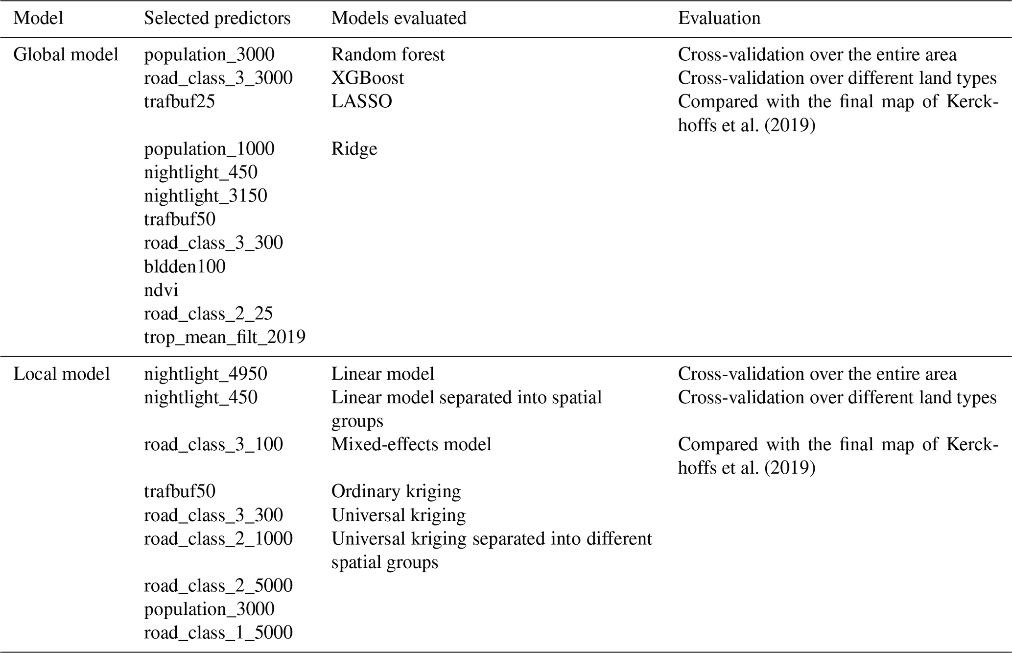
Table 5 Features of the global and local models regarding model complexity and how the spatial component is considered.

Evaluations of the different linear and nonlinear models were carried out using repeated random sampling validation (i.e., Monte Carlo cross-validation) performed 20 times. In each iteration, 90 % of the data was used for training and the remaining 10 % for testing. For testing model performance on spatial groups, 30 testing samples were used every time (Boersma, 2025a). This approach allowed us to evaluate the variance and median statistics for each model in terms of R², MAE, and RMSE (Fig. 4). The repeated sampling provided stable estimates.

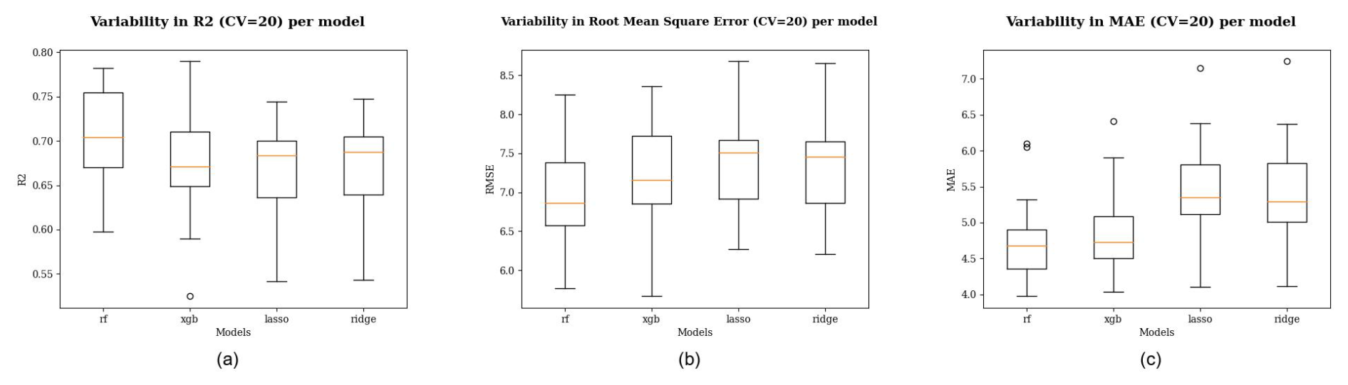
Figure 4 Out-of-sample performance evaluated using random sampling validation repeated 20 times. The metrics shown are R² (a), RMSE (b), and MAE (c). Upper and lower quartiles indicate variability. RF = random forest, XGB = XGBoost.

3 Results

3.1 Global models

When comparing out-of-sample performance via 20-fold repeated random sampling validation, the linear models (i.e., LASSO and ridge) exhibited performance similar to that of the nonlinear models, particularly in terms of R². Among the models, the random forest consistently outperformed the others, with the highest median R², lowest RMSE, and lowest MAE. The robustness of the random forest model is further emphasized by its minimal standard deviation in R² and MAE (Fig. 4).

3.1.1 Accounting for spatial information

We further investigated the influence of spatial heterogeneity by comparing model performance across different spatial groups using the global dataset. Descriptive statistics for NO₂ concentrations in each spatial group reveal distinct differences (Table 6).

Table 6 Descriptive statistics of NO₂ concentrations for each spatial group (in µg m⁻³).

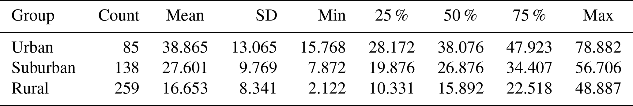
Table 7 Model performance per spatial group (Monte Carlo CV, number of iterations = 20, and 30 samples used for testing per iteration). RMSE and MAE are represented as NO₂ (in µg m⁻³).

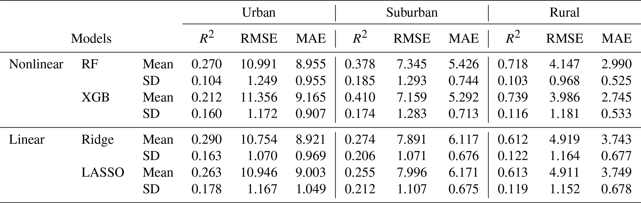
Table 8 Model performance using leave-one-out cross-validation.

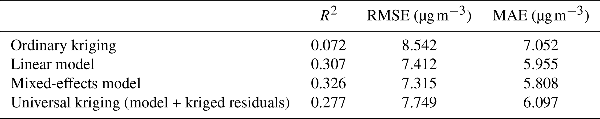
Table 7 details the performance metrics (R², RMSE, MAE) for each spatial group. Nonlinear models outperformed linear ones in suburban and rural areas, while performance was less distinguishable in urban areas, likely due to the smaller sample size. Ensemble-tree-based methods, such as the random forest, showed lower accuracy in urban areas, possibly due to the limited and heterogeneous nature of the data in this group.

3.1.2 Spatial prediction patterns

Figure 5 presents the spatial predictions of NO₂ concentrations across the Amsterdam area for each model. Panels (a) and (b) depict the predictions from nonlinear models, while panels (c) and (d) illustrate the results from linear models. Generally, linear models exhibit a higher tendency to overfit, as their prediction maps are more influenced by extreme values (i.e., concentrations below 15 or above 50 µg m⁻³) compared to the nonlinear techniques. Interestingly, the linear models identify a significant NO₂ hotspot in the southwestern part of the study area, which is not captured by the nonlinear models. Across all models, however, elevated NO₂ is consistently observed along major roads and in some urban areas, such as Haarlem (see Fig. S18).

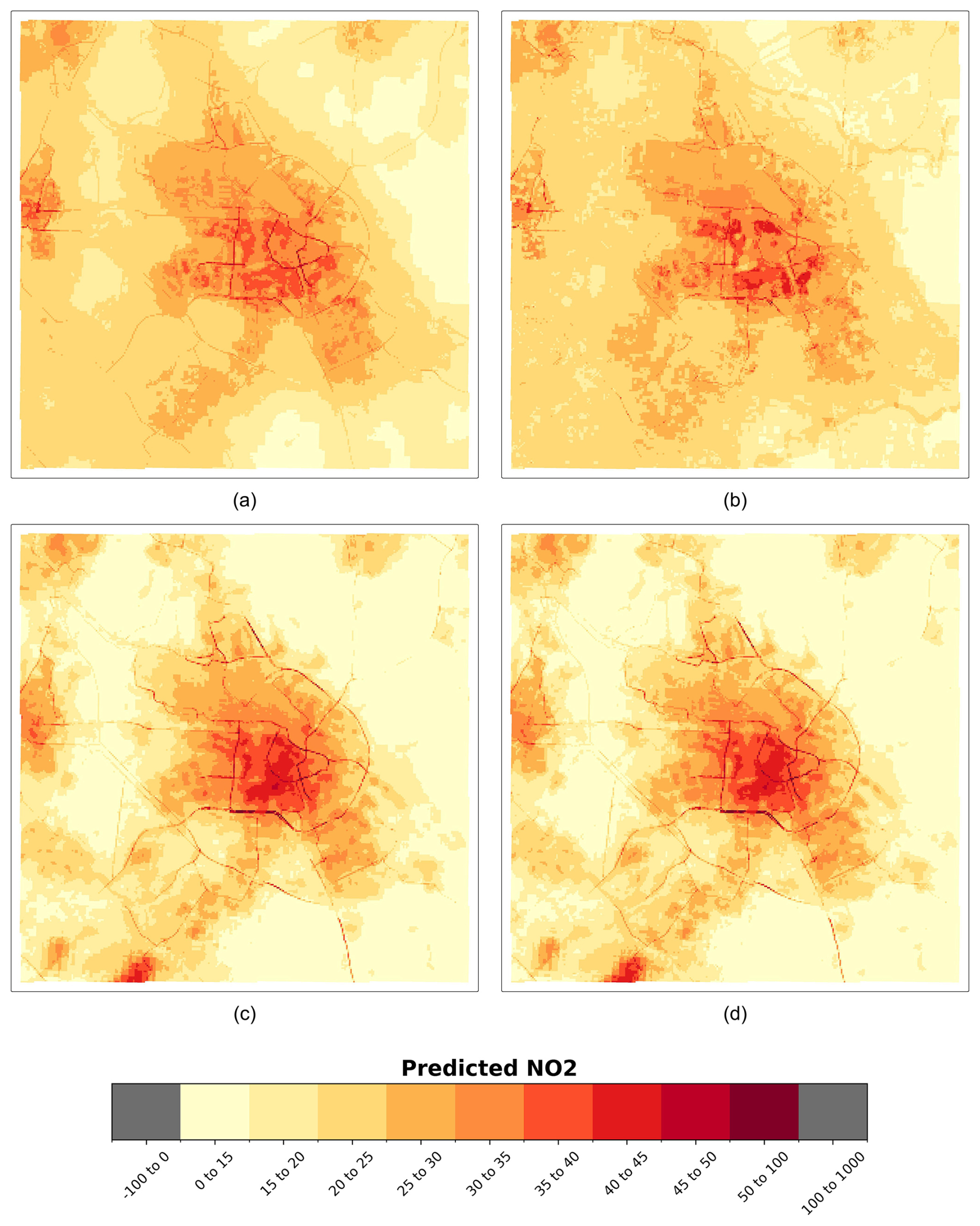
Figure 5 Spatial patterns of predicted NO₂ (100 m), measured in µg m⁻³, nonlinear global models for Amsterdam. (a) Random forest and (b) XGBoost. The linear models are (c) LASSO and (d) ridge. The area is 30 km×30 km.

Figure 6 shows the spatial patterns of predicted NO₂ concentrations for Hamburg (a, b), Utrecht (c, d), and Bayreuth (e, f) using the random forest and ridge regression models. Predictions from other models (XGBoost, LASSO, LightGBM) for these cities, including both zoomed-in and zoomed-out views, are provided in Figs. S19–S30.

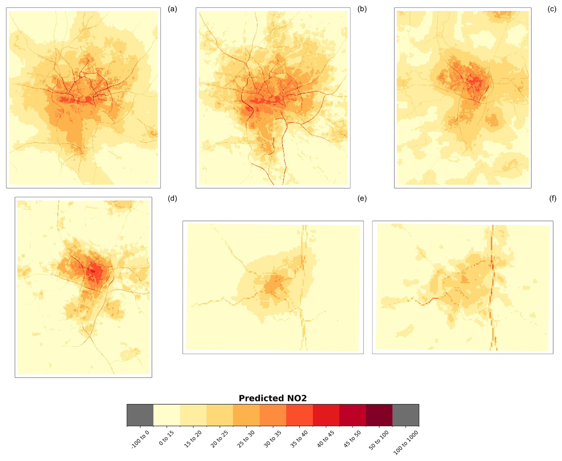
Figure 6 Spatial patterns of predicted NO₂ (100 m), measured in µg m⁻³, per global model for Hamburg (area: 30 km×30 km), Utrecht (area: 25 km×25 km), and Bayreuth (area: 10 km×10 km) – (a) random forest (Hamburg), (b) ridge (Hamburg), (c) random forest (Utrecht), (d) ridge (Utrecht), (e) random forest (Bayreuth), and (f) ridge (Bayreuth).

Comparing the prediction maps of these cities reveals noticeable differences in spatial patterns. A key finding is that in Hamburg, the highest air pollution levels are concentrated around major roads, while in Utrecht, the urban center exhibits the highest NO₂ concentrations. This correlation between major roads and elevated air pollution in Hamburg can be reasonably explained by the city's high traffic congestion, as it ranks 69th among the most congested cities globally (Tomtom, 2021). Interestingly, there are also spatial differences in the predicted NO₂ concentrations along highways between the random forest and ridge models. For instance, in Hamburg, the ridge model predicts high NO₂ levels along highways in the southeastern and western parts of the city, whereas the random forest model provides a more nuanced spatial identification of these areas. The random forest predictions highlight more pronounced air pollution along roads in the central and northern parts of Hamburg compared to the ridge model.

Furthermore, the magnitude of high pollution levels related to major roads is significantly greater in Hamburg than in Utrecht and Bayreuth. Nevertheless, the relationship between the presence of roads and higher air pollution levels is evident in both Utrecht and Bayreuth, particularly in the predictions from the ridge model. In Utrecht, the urban center is more prominently identified as a high NO₂ concentration area compared to in Hamburg and Bayreuth. Additionally, the ridge model for Utrecht shows more clusters of elevated NO₂ levels in the periphery, whereas the random forest model predicts a more scattered distribution of NO₂ concentrations in the urban center, similar to the pattern observed in the Amsterdam area.

Bayreuth, on the other hand, is characterized by moderate NO₂ pollution, with very low NO₂ concentrations (<15 µg m⁻³) in the rural areas surrounding the city. However, some clusters of higher NO₂ levels exceeding the 15 µg m⁻³ benchmark are observed in the vicinity of other villages, suggesting a relationship between population or building density and air pollution (see also Figs. S25–S27). Figure S31 provides the distribution of predicted NO₂ concentrations for each global model and location.

3.2 Local models

The performance of the local models was assessed using the R², RMSE, and MAE metrics. Table 8 summarizes the performance of the linear model, mixed-effects model, ordinary kriging model, and universal kriging model, all evaluated using leave-one-out cross-validation. Among these, the ordinary kriging model exhibits the poorest performance. Figure 7 illustrates the spatial prediction patterns for each model. Notably, the universal kriging model outperforms the ordinary kriging model significantly. However, note that with the ordinary kriging model, we could see the smoothed spatial patterns of the air pollution measurements. The simple linear model surpasses the universal kriging method in terms of prediction accuracy. Incorporating spatial groups as random effects in the mixed-effects model leads to a higher R² and lower RMSE and MAE, indicating the importance of accounting for spatial heterogeneity.

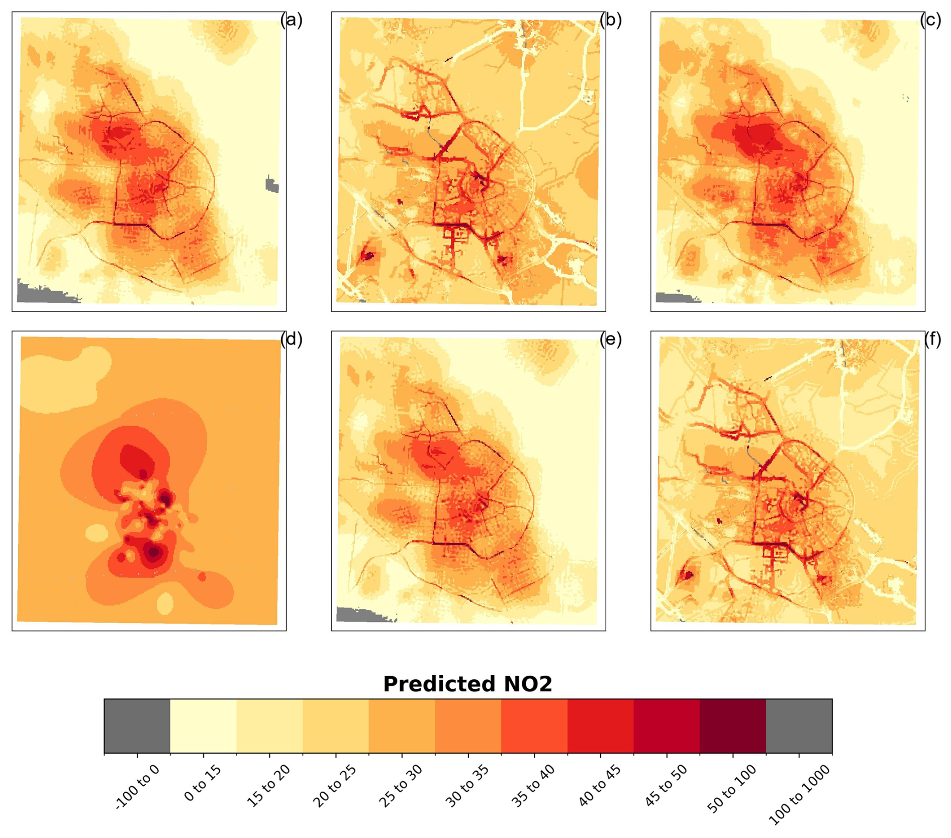
Figure 7 Spatial patterns of predicted NO₂ (µg m⁻³) at a 100 m resolution based on the local dataset – (a) linear model, (b) linear model separating for spatial groups, (c) mixed-effects model, (d) ordinary kriging, (e) universal kriging, and (f) universal kriging separating for spatial groups.

Table 9 Model performance per spatial group (CV = leave-one-out cross-validation). RMSE and MAE are in µg m⁻³.

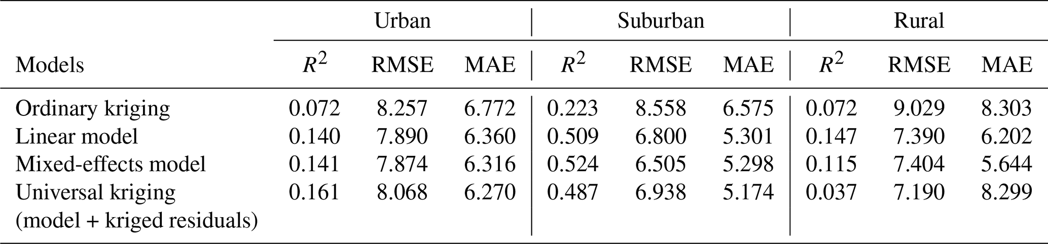
Table 9 provides model performance metrics for each spatial group, again using leave-one-out cross-validation. Consistent with the global model results, local models trained on urban observations tend to perform poorly. This poor performance is likely caused by an imbalance between the relatively small number of samples and the relatively high heterogeneity. This imbalance may hinder the models' ability to capture the variability within urban areas, contributing to their poorer performance in this group. Interestingly, proximity to roads does not necessarily correlate with model performance, as the suburban group exhibits a higher R² than the rural group. Unlike global models, which perform best in rural areas, local models perform best in suburban areas. This difference may arise because observations in rural areas within the local dataset are more similar to those in urban and suburban areas than in the global dataset due to a more uniform distribution of predictor values.

3.3 Spatial prediction patterns

Figure 7 displays the predicted NO₂ patterns based on the local dataset. The prediction map for the linear model (panel a) is quite similar to those for the mixed-effects (panel c) and universal kriging (panel e) models, with all identifying a high-NO₂-concentration cluster in the northwestern part of Amsterdam. Further analysis suggests that this cluster is likely influenced by the predictor “road class 2 5000” (i.e., the number of primary roads within each 5000 m buffer), as this predictor exhibits a similar cluster in the same location (see Figs. S32–S41).

The two models that account for spatial groups before the modeling process (mixed-effects and universal kriging) display comparable patterns, where the influence of roads is evident through either the predictors themselves or the spatial groupings (see also Fig. S42). The relatively low NO₂ values along roads in the outer Amsterdam area can be attributed to the spatial grouping. High standard deviations in predictor values within a specific spatial group can affect that group's NO₂ predictions, potentially leading to overestimation or underestimation in certain areas.

The high NO₂ values along roads are primarily associated with the suburban spatial group, where the observations are located within 100 m of the roads. Compared to the rural group, the data distribution for each predictor in the suburban group is substantially different, leading to distinct learning patterns that explain the relatively high prediction values along roads (see Figs. S43–S51). In some instances, negative predicted values are observed, albeit rarely. These may result from discrepancies in feature characteristics between the training and testing datasets.

Comparing local prediction patterns to global prediction patterns reveals that the local models identify a cluster of high air pollution in the northwestern part of Amsterdam that the global models do not detect. This discrepancy could be due to differences in the spatial distribution of NO₂ values between the local and global datasets, leading to distinct learning patterns in the respective models (Fig. 1). Moreover, Figs. 5 and 7 underscore the challenge of comparing spatial variations between global and local models, given their differing algorithms. Local models, with their focus on specific spatial groupings and detailed predictors, capture regional clusters that global models may overlook or underrepresent due to their broader scope.

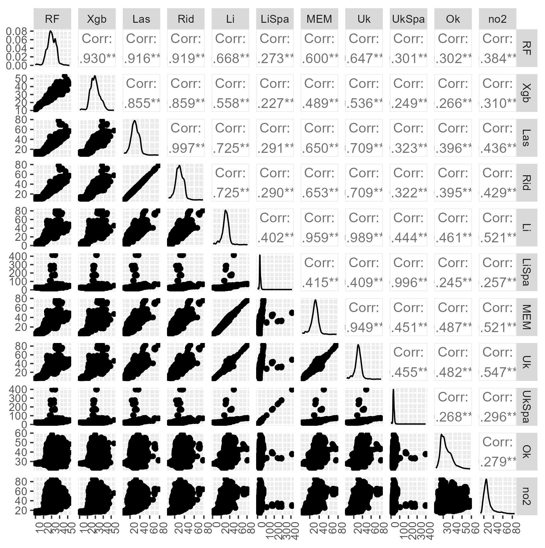
Figure 8 Comparing model predictions whereby the numbers equal the Pearson correlation coefficient. RF: random forest, XGB: XGBoost, LR: linear regression, LRsp: linear regression accounting for spatial groups, MEM: mixed-effects model, UK: universal kriging, UKsp: universal kriging accounting for spatial groups, OK: ordinary kriging, no2: mobile NO₂ map from Kerckhoffs et al. (2021).

3.3.1 Model comparison

Figure 8 shows the correlation in predicted NO₂ values for the local and global models, as well as the mobile NO₂ map from Kerckhoffs et al. (2019) (referred to as the open-NO₂ dataset), which was used as a benchmark (Fig. S53). To improve the clarity of the correlations between the models and the open-NO₂ dataset, we addressed some extreme prediction values. These outliers were removed to prevent them from skewing the analysis and to provide a more accurate representation of the correlations. We selected a manual threshold of 85 as the upper bound based on the maximum value observed across the 10 models (excluding the 2 where outlier detection was applied first). The lower bound was set to 0. The correlation matrix with these extreme predictions removed (including LightGBM results) is shown in Fig. S54. The global models are highly correlated, with the LASSO model being the least correlated with other global models. The correlations between the ordinary kriging model and other models are low, which is expected, as the covariance function has a small length scale. Although the assumption of second-order stationarity is likely violated in ordinary kriging due to the strong influence of local traffic on NO₂ concentrations, the method remains applicable. It still provides the best linear unbiased prediction (BLUP) based on Euclidean distances between spatial coordinates. When comparing the models with the open-NO₂ dataset, some local models show more similarity than global models do. This is reasonable, as the local model dataset is also from Amsterdam. Table 10 shows the residuals per global and local model. The XGBoost model emerged as the most accurate among the global models, with the lowest mean residual (1.36), indicating that it closely matched the open-NO₂ values. The LASSO model also demonstrated higher residuals compared to XGBoost and ridge, suggesting less consistency in its predictions. In contrast, local models exhibited greater variability in residuals. The mixed-effects model and universal kriging had relatively moderate mean residuals (2.51 and 1.83, respectively), while the linear spatial group and universal kriging spatial group models had significantly higher standard deviations, indicating more extreme residuals. Ordinary kriging retained the highest mean residual (4.71), reinforcing the trend that local models generally had greater prediction errors compared to global models. A spatial comparison of the predicted NO₂ concentration values between the open-NO₂ dataset and the global and local models is shown in Figs. S55–S59 and S60–S65, respectively. A spatial comparison of the global and local model predictions with the measurement station data can be found in Figs. S66–S85 and S86–S91, respectively.

Table 10 The summary statistics of the differences between model predictions and the mobile-measurement-derived NO₂ map from Kerckhoffs et al. (2021).

4 Discussion

Several studies have applied statistical modeling to ground station measurements and geospatial predictors for NO₂ mapping, but the impact of spatial heterogeneity, as well as a thorough analysis of the prediction patterns in different areas using different models, has often been under-stressed. In this study, we address this gap by comparing spatial and non-spatial models across different spatial scales. Below, we discuss the key findings and provide our perspectives.

4.1 Relationship between predictors and other pollutants

For both global and local datasets, traffic and population density emerge as the most influential predictors, aligning with the findings of Beelen et al. (2013), which emphasize the importance of these variables for improving prediction accuracy. The strong influence of traffic on NO₂ concentrations also supports the conclusions of Lu et al. (2020) and Chen et al. (2019). However, since the pollutant sources vary (Chen et al., 2019), the modeling results for NO₂ may not be directly applicable to other pollutants.

4.2 Accounting for spatial groups

Without accounting for the spatial groups, the differences in terms of the accuracy assessment matrices between linear and nonlinear techniques are minimal. The random forest model generally performs with the highest R² and lowest MAE, and the R² of the ridge model is higher than that of the XGBoost model. When accounting for spatial groups, the differences in model performance between linear and nonlinear techniques become more pronounced, with nonlinear models generally outperforming linear models, particularly in rural areas where data are more homogeneous.

A limitation of the data is the fact that the most heterogeneous group (urban) is the least represented in terms of the number of data points, at least for the global dataset. In urban areas, the more heterogeneous nature of the data reduces the performance gap between linear and nonlinear techniques, with both performing poorly. This poor prediction accuracy in urban areas is concerning, as the impact of air pollution is often more severe in these regions due to proximity to traffic-heavy roads and industrial areas (He et al., 2022). Although spatial grouping improves predictive reliability, it can lead to counterintuitive patterns, such as lower predicted NO₂ concentrations along roads compared to in the surrounding rural areas. In the local dataset, the threshold for defining “urban” areas was adjusted from the upper 75 % (0.75) to the median (0.5). This adjustment was necessary due to the limited sample size, which required a broader definition to ensure sufficient data coverage for urban areas. However, this change also resulted in a less stringent definition of “urban,” potentially including areas with lower population densities. While this adjustment expands the number of training samples available for the most heterogeneous group (urban), it introduces a limitation by diluting the urban group and affecting the comparability of results. This trade-off underscores the challenges of balancing data representation with statistical robustness in spatial analyses.

4.3 Influence of cross-validation techniques

The cross-validation (CV) strategy plays a crucial role in model performance and generalizability. In this study, we opted for a random $\mathrm{90}/\mathrm{10}$ training–testing split repeated 20 times to ensure model stability while maintaining sufficient training data. For testing on spatial groups, we further limited the testing samples to 30 to account for spatial variability and avoid data imbalance. This approach allows us to evaluate model performance across different spatial settings while mitigating the risk of overfitting.

However, the random split employed in this approach can lead to biased performance estimates, particularly with small datasets. Some points may be used multiple times, while others might not be used at all, which can skew results. To address this issue, alternative strategies like the 5-fold CV are often employed, as they provide a good balance between bias and variance. In the 5-fold CV, the dataset is divided into five partitions, ensuring that each point is used for validation exactly once. This method can be particularly useful when the dataset is small, as it ensures more comprehensive utilization of the data.

In our study, we chose to use the Monte Carlo CV because it provides a robust measure of uncertainty, particularly for relatively small datasets. The Monte Carlo CV works well when data are limited, as it generates multiple datasets through resampling, allowing us to estimate variability and model performance more effectively. The Monte Carlo CV aims to reduce bias by randomly drawing training points for each iteration, thus providing a more reliable estimate of model accuracy. Although increasing the number of iterations and reducing the testing set size could further reduce bias, leaving more data points in the testing set offers additional information about the model's performance.

Alternative techniques, such as the 5-fold CV, remain popular because they offer a straightforward balance between training and validation data. Nonetheless, the Monte Carlo CV may provide better estimates of uncertainty, especially in cases with limited data, which could make it preferable for heterogeneous spatial datasets. Although increasing the number of iterations may improve predictive reliability, the trade-off between computational efficiency and statistical robustness must be carefully considered.

Meyer and Pebesma (2021, 2022) criticized the imprudent use of global-scale models, in particular highlighting the issue that model performance cannot be validated in regions without observational data. They advocate for the use of spatial cross-validation to address this limitation. After careful consideration, we opted for the Monte Carlo CV to mitigate the bias introduced by spatial cross-validation (Wadoux et al., 2021; Lu et al., 2023). We would like to emphasize that the core issue in cross-validation for spatial modeling lies in the inclusion of spatial coordinates or distances as predictors. From this perspective, it is evident that sampling should be random in the predictor space. Therefore, we argue that cross-validation in spatially correlated data is not fundamentally different from standard cross-validation, provided that the predictor space sampling is handled appropriately.

4.4 Global and local predictions

In comparing global and local models, each approach has distinct strengths and limitations. Local models, tailored to specific spatial groupings and incorporating detailed predictors, excel at capturing regional clusters and nuances. These models can identify patterns and variations that broader, global models might miss or represent inadequately. On the other hand, global models are designed to capture overarching trends across larger areas but often overlook the finer local details crucial for accurate predictions in specific regions.

The findings of Yuan et al. (2023) support this distinction, highlighting the fact that integrating large-scale stationary measurements with local mobile data improves modeling performance in urban areas by accounting for finer spatial variations. Their study underscores the limitations of global models, which, while providing a broad overview, may fail to capture the detailed local variations necessary for precise predictions. By combining global and local data, a more accurate and nuanced depiction of air pollution can be achieved, particularly in complex urban environments where local details are critical.

4.5 Spatial variation in feature importance

The influence of specific predictors on NO₂ concentrations can vary significantly between cities. For example, building density and population are more significant contributors to air pollution in Utrecht, whereas traffic has a greater impact on high NO₂ concentrations in Hamburg. Applying global models with the same predictors across different cities may conceal this finding and yield suboptimal results. It is therefore important to consider the spatial heterogeneity and at the same time ensure a consistent uncertainty assessment. However, the current number of official ground stations may not be sufficient to characterize the spatial heterogeneity and ensure a detailed and reliable prediction.

4.6 Further perspectives on model improvement

The limited number of observations in the local dataset poses challenges for fitting complex models. Transforming the original data could potentially avoid predictions falling outside the plausible range (e.g., below 0 µg m⁻³). However, in this study, a transformation was not applied for the following reason. Although airborne pollutant concentrations are often positively skewed (Maranzano et al., 2020), Lu et al. (2023) found that optimal modeling results were obtained without transforming the data and by using a Gaussian likelihood – even when other distributions, such as gamma, better reflected the data's skewed distribution. Moreover, while the LASSO and ridge models perform well with the global dataset, their predictions were less satisfactory with the local dataset. In this study, traffic volumes were a significant feature, yet no distinction was made between different types of traffic (e.g., cars, buses, trucks), vehicle types (e.g., electric, diesel), or engine types, all of which are known to influence air pollution (Wong et al., 2021). For example, distinguishing between vehicle types could reveal that certain roads, such as those leading to or from the port of Hamburg, have a higher proportion of trucks, which might explain localized clusters of high NO₂ concentrations.

5 Conclusions

In this study, we investigate the spatial heterogeneity of NO₂ modeling by comparing various linear and nonlinear statistical models at different scales (local vs. global). One of the key findings of this study is that the model performance matrix varies trivially with models of different levels of complexity but significantly when considering spatial heterogeneity and modeling in various population, traffic, and urban settings. The nonlinear techniques have better predictions in rural and suburban areas compared to the linear models. Global model prediction accuracy is considerably higher in rural, homogeneous areas, the influence of which leads to high overall performance without accounting for spatial groups. Methods preferred in global modeling could be unfavorable in local modeling. The relatively few NO₂ observations and potentially lower quality of the local (Palmes) dataset compared to the official ground station measurement are important reasons for the unsatisfactory performance of nonlinear models. Using the local dataset, we also found that explicitly accounting for spatial autocorrelation in the universal and ordinary kriging models does not improve accuracy; however, analyzing predictions across spatial groups provides valuable insights. Also, different modeling techniques lead to different NO₂ clusters in the prediction map despite the similar performance matrices that they received. Last but importantly, our results suggest that focusing solely on overall prediction accuracy can lead to overconfidence and to an underestimation of the further efforts required in statistical air pollution mapping.