OpenBench: a land model evaluation system

Recent land surface models (LSMs) have evolved significantly in complexity and resolution, requiring comprehensive evaluation systems to assess their performance. This paper introduces the Open Source Land Surface Model Benchmarking System (OpenBench), an open-source, cross-platform benchmarking system designed to evaluate the state-of-the-art LSMs. OpenBench addresses significant limitations in the current evaluation frameworks by integrating processes that encompass human activities, facilitating arbitrary spatiotemporal resolutions, and offering comprehensive visualization capabilities. The system utilizes various metrics and normalized scoring indices, enabling a comprehensive evaluation of different aspects of model performance. Key features include automation for managing multiple reference datasets, advanced data processing capabilities, and support for station-based and gridded data evaluations. By examining case studies on river discharge, urban heat flux, and agricultural modeling, we illustrate OpenBench's ability to identify the strengths and limitations of models across different spatiotemporal scales and processes. The system's modular architecture enables seamless integration of new models, variables, and evaluation metrics, ensuring adaptability to emerging research needs. OpenBench provides the research community with a standardized, extensible framework for model assessment and improvement. Its comprehensive evaluation capabilities and efficient computational architecture make it a valuable tool for both model development and operational applications in various fields.

1 Introduction

Land surface models (LSMs) simulate the complex interactions among the land surface, planetary boundary layer, rivers and lakes, glaciers and frozen soils, plant physiology and ecology, vegetation dynamics, biogeochemistry, human activities, and other processes occurring on the land surface (Blyth et al., 2021; Dai et al., 2003; Lawrence et al., 2019; Pokhrel et al., 2016). These models play an important role in understanding and predicting various changes in the Earth system, serving as a bridge connecting the land surface, ocean, and atmosphere (Fisher and Koven, 2020; Ward et al., 2020; Liu et al., 2024). As such, they are key components of Earth system models (ESMs) and have significant impacts on our ability to comprehend and predict weather, climate, hydrological cycles, carbon cycles, and various other environmental factors. In recent decades, LSMs have undergone rapid development, evolving from basic “bucket” models (Manabe, 1969) to advanced multi-module systems (Blyth et al., 2021) that incorporate both biogeochemical processes (e.g., greenhouse gas, carbon, nitrogen, and phosphorus cycles) and geophysical processes (including land-use changes, three-dimensional surface water, subsurface flow, and flooding), as well as human activities (such as agriculture, reservoir management, and urban development). This evolution has been driven by advances in hydrology, meteorology, computer science, and measurement technology, leading to the development of increasingly complex models. Concurrent with the increasing complexity of processes represented in LSMs, there has been a significant improvement in spatial resolution as well. Models have progressed from traditional forecasting scales of 25–100 km (Dai et al., 2003) to current fine scales of 0.1–10 km (Chen et al., 2024). The increasing complexity and resolution of models require a comprehensive evaluation and analysis of simulation results.

Table 1 The software that can be used or partly used for land surface model evaluation. The abbreviations for specific nouns in the table are described as follows: AMWG – NCAR's CAM Diagnostics Package; CVDP – NCAR's Climate Variability Diagnostics Package; ESMValTool – Earth System Model Evaluation Tool; PMP – PCMDI's Metrics Package; ILAMB – International Land Model Benchmarking System; MDTF – NOAA's Model Diagnostics Task Force Framework; MPAS-Analysis – analysis for MPAS (Model for Prediction Across Scales) components of E3SM Ocean and Sea-ice analysis for E3SM's MPAS components; E3SM Diags v2.7 – The E3SM Diagnostics Package; AMBER – Automated Model Benchmarking; PALS – Protocol for the Analysis of Land Surface models; LVT – Land Surface Verification Toolkit; benchcab – evaluation tool for the land surface model CABLE; TraceMe – traceability analysis system for model evaluation; AMET – Atmospheric Model Evaluation Tool; MET – Model Evaluation Tool; MVIETool – Multivariable Integrated Evaluation Tool.

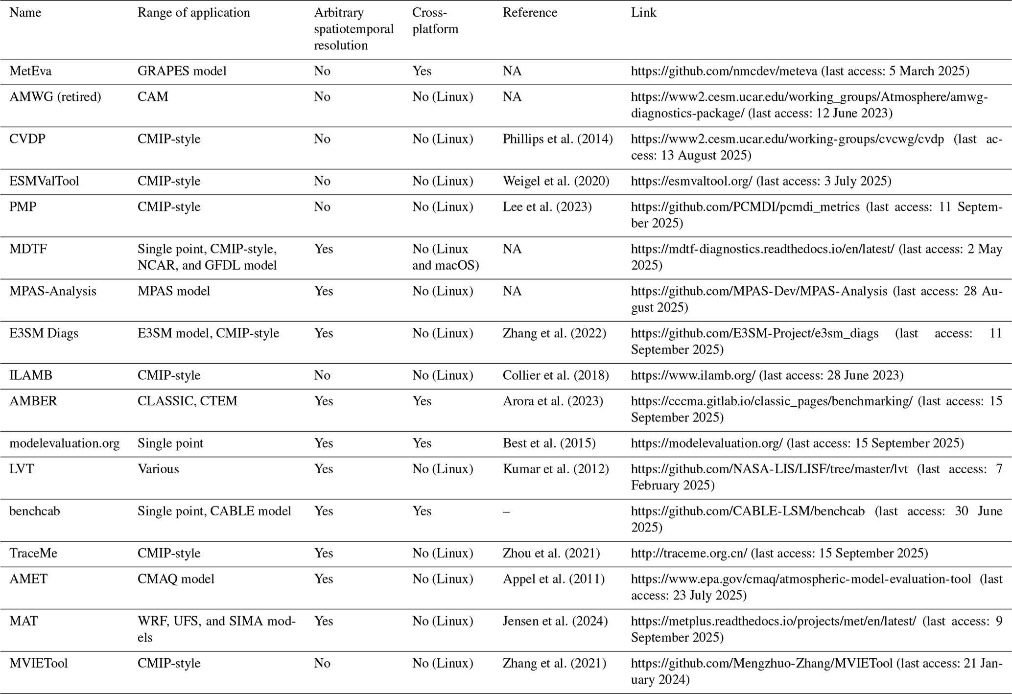
In recent years, various model benchmarking systems (see Table 1) have been developed. These systems assess model performance in comparison to multiple sources of reference datasets. Most of these benchmarking systems consist of benchmark datasets, evaluation software, metrics, model operating environments, and auxiliary tools. The benchmark datasets standardize observation, reanalysis, and remote sensing data to evaluate model accuracy in simulating land processes. Evaluation software includes metrics, execution environments, and tools designed for automated assessment and quantifying LSMs' performance. The operating environment comprises the software and hardware for running evaluations, while ancillary tools support benchmarking. Despite the importance of LSM evaluation and the development of various benchmarking systems, several limitations persist in current evaluation approaches. These limitations have become increasingly apparent as the complexity and resolution of LSMs have increased. One significant area for improvement is the scope of evaluation variables in most existing evaluation systems. These systems typically focus on some range of commonly used variables, such as water, heat and carbon fluxes, temperature, and vegetation coverage. This restricted scope fails to capture the full range of processes simulated by modern LSMs. For instance, TraceMe (Zhou et al., 2021) is primarily designed to evaluate model outputs related to the carbon cycle, while the MetEva software developed by the National Meteorological Center of China (https://github.com/nmcdev/meteva, last access: 5 March 2025) focuses on meteorological fields. However, neither of these tools provides a comprehensive assessment of land surface processes, nor can they easily adapt to new evaluation indicators or datasets. In particular, there is a lack of comprehensive evaluation for hydrological cycles and human activities, making it challenging to fully assess model performance in these critical areas. Human activity, while an important factor affecting surface processes, is one of the most challenging aspects to model and evaluate. This is primarily due to the small-scale nature of human activity data (e.g., crop yields, dam operation, and anthropogenic heat) and the involvement of complex socio-economic and land-use change data. These datasets are often multi-source, complex, and highly uncertain. To date, no evaluation system has been found to integrate the assessment of human activities in LSMs broadly.

Another significant challenge in current LSM evaluation practices is the difficulty in conducting inter-model comparisons. This comparative work is a key step in improving model performance and understanding model differences and uncertainties. However, the lack of a universal and comprehensive evaluation tool presents significant challenges, especially in the context of high-resolution complex models and evolving underlying datasets. Traditionally, software tools for evaluating LSMs have often been customized for specific models or datasets. For example, the evaluation tools for the Canadian Land Surface Scheme (CLASS) (Verseghy, 1991) and the Community Atmosphere Biosphere Land Exchange (CABLE) model (Haverd et al., 2018), i.e., AMBER (Arora et al., 2023) and benchcab (https://github.com/CABLE-LSM/benchcab, last access:30 June 2025), are optimized for their respective outputs. Customized software designs lead to several issues. Researchers must invest time in learning specific usage methods and data formats for each new model, limiting their ability to try new models and slowing down comparisons. Different tools using different evaluation criteria and formats make it difficult to compare model performance. Evaluation tools like the International Land Model Benchmarking (ILAMB) platform (Collier et al., 2018) require complex data processing, such as converting model outputs to the Coupled Model Intercomparison Project (CMIP) standard. This process consumes time and computing resources, increasing the risk of errors and potentially affecting the reliability of evaluations. In the meantime, some platforms, such as ILAMB and the Land Surface Verification Toolkit (LVT) (Kumar et al., 2012), offer a wide range of assessments for process variables. However, their spatiotemporal resolution is relatively low (typically at a monthly scale and 0.5°). They have limitations in processing data conversion at different scales, making it difficult to perform simulation evaluations at multiple spatiotemporal scales.

Visual analysis capabilities are another area where current evaluation tools often fall short. Many lack visual functions or produce low-quality visualizations, making it difficult to display evaluation results effectively. For instance, while some can produce graphical diagnostics, the quality is often insufficient to meet publication standards, and it is unable to customize output. Platform compatibility is also a significant issue, as most evaluation tools are designed to run only on Linux. This limits their application on Windows or macOS operating systems, thus restricting their popularity and accessibility.

To address these challenges and meet the high standard requirements of new-generation LSM verification and evaluation, we have developed OpenBench (Open Source Land Surface Model Benchmarking System). The core goal of OpenBench is to provide an open-source, fast, efficient, diverse, and accurate evaluation mechanism for high-resolution land-surface model outputs. OpenBench is designed as a universal and high-performance LSM evaluation system, fully written in Python, that realizes functions such as data processing, evaluation method encapsulation, and result analysis visualization. OpenBench supports cross-platform operation, including Windows, macOS, and Linux, enhancing its accessibility and usability across different research environments. OpenBench incorporates evaluation metrics and datasets that account for human activities on land surface processes, filling a significant gap in current evaluation systems. The system provides a unified and standardized benchmark test method framework, allowing for efficient and comprehensive validation and evaluation of typical land surface models, such as CoLM, CLM, Noah-MP, GLDAS, and JULES, as well as CMIP-style model output. By ensuring the widespread sharing of evaluation results, OpenBench aims to advance scientific research and operational work in land surface modeling. The system maximizes the use of available observational and reanalysis data through its efficient data management and processing capabilities.

In the following sections of this paper, we will detail the methodology behind OpenBench, including its system architecture, its key components, and the benchmark datasets developed for it. We will then present case studies that demonstrate its application in evaluating and comparing different LSMs or parameterizations, highlighting its capabilities in handling high-resolution data and complex processes. Finally, we will discuss the implications of this new evaluation system for the field of land surface modeling and outline future directions for its development and application.

Figure 1 General flowchart of OpenBench.

2 Overall structure

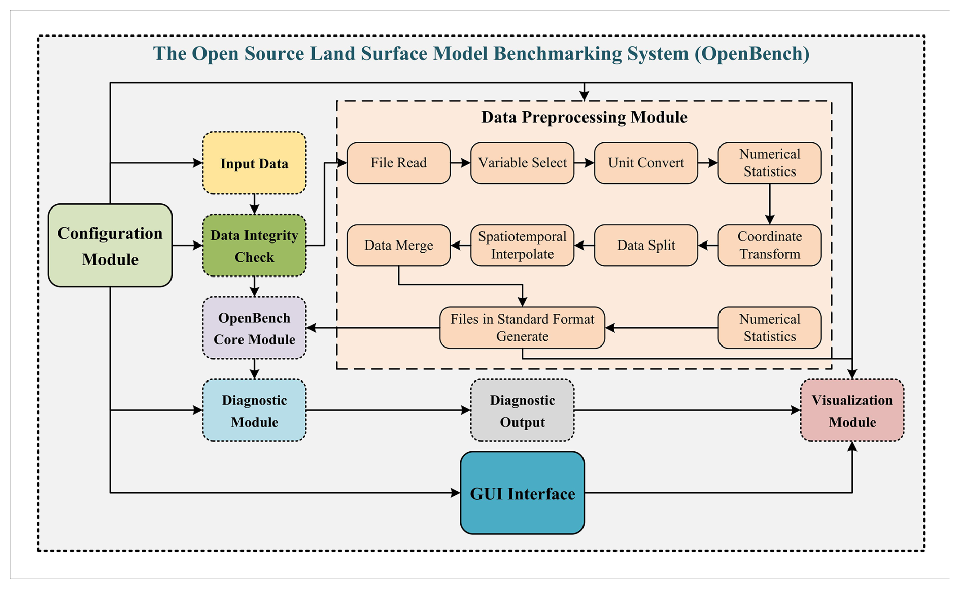
OpenBench represents a significant advancement in the field of model evaluation and intercomparison. This section outlines the system's overall structure, highlighting its key components and workflow. OpenBench is designed with modularity and flexibility in mind, enabling efficient processing of diverse datasets and model outputs. The OpenBench code is designed to simultaneously handle various data types, including plot-scale data (such as station data) and gridded data (regional or global) for both simulation and reference datasets. The flowchart of OpenBench is shown in Fig. 1.

The system includes six components: configuration management, data processing, evaluation, comparison processing, statistical analysis, and visualization. The configuration management module accommodates three configuration namelist formats (YAML, JSON, and Fortran namelist) to meet different user preferences and workflows, with JSON as the default format. Users can utilize the configuration namelist to define evaluation parameters, data sources, and model outputs. This adaptable configuration system facilitates straightforward customization of evaluation scenarios. The data processing module handles the preprocessing of both reference and simulation data, including temporal and spatial resampling to ensure consistent comparison between datasets with different spatiotemporal resolutions. The evaluation module implements the core evaluation logic, applying various metrics and scores to quantify model performance. It supports both gridded and station-based data and adapts its methods accordingly. The comparison module facilitates multi-model and multi-scenario comparisons, enabling comprehensive analysis across different models or configurations. Finally, advanced statistical techniques are implemented in the statistical analysis module, providing deeper insights into model behaviors and performance patterns. The system also includes capabilities for generating visualizations of evaluation results, which are crucial for interpreting and communicating findings provided in the visualization module.

The system's workflow follows a logical sequence of operations. The process begins with initialization, where command-line arguments are parsed and configuration files are read. This stage sets up necessary directories and initializes key variables, laying the groundwork for subsequent operations. The system then moves into the data preparation phase, where both observational and model data are processed to ensure compatibility in terms of temporal and spatial resolution. This crucial step handles various data formats and structures, normalizing them for consistent analysis. At the core of the system is the evaluation process. Here, a wide array of metrics and scores is applied to quantify the agreement between model outputs and observational data. This step is highly parallelized to efficiently handle large datasets, allowing for a comprehensive assessment across multiple variables and time frames. If multiple models or scenarios are being evaluated, the system performs comparative analyses to highlight relative strengths and weaknesses. This comparison stage provides valuable perspectives into model performance across different conditions or implementations. Following the primary evaluation, the system conducts advanced statistical analyses to gain a profound understanding from the evaluation results. This may include uncertainty quantification, trend analysis, or other sophisticated statistical methods. The final stages involve result generation and visualization. The system compiles evaluation results, generates summary statistics, and prepares data for visualization. The system can produce various charts, graphs, and maps to effectively communicate the evaluation outcomes. Throughout these stages, the system demonstrates flexibility in handling different types of data (grid-based or station-based), various temporal resolutions, and a wide range of environmental variables. It also incorporates specialized handling for different land surface models, recognizing the unique characteristics and outputs of each. This comprehensive approach allows for a thorough, standardized evaluation of land surface models, providing valuable feedback for model development and application in Earth system science.

Nevertheless, OpenBench is developed to serve as a specialized tool for land surface model output analysis, evaluation, and comparison. The software package is freely available to the community. The code is modular and can be easily extended or modified to accommodate the specific requirements of different evaluation tasks. OpenBench relies on various popular and well-established Python packages specific to the scientific computing stack: NumPy (Harris et al., 2020), Xarray (Hoyer and Hamman, 2017), Pandas (Mckinney, 2010), SciPy (Virtanen et al., 2020), Matplotlib (Hunter, 2007), Cartopy (Elson et al., 2024), Dask (Rocklin, 2015), and Joblib (Joblib, 2020). For the remap functions, there are several options: SciPy, Cdo (Schulzweida, 2022), xESMF (Zhuang et al., 2023), and xarray-regrid (Schilperoort et al., 2024) are available for selection. We use as few packages as possible, reducing dependencies to improve performance and compatibility. The software is developed and hosted on GitHub and is distributed under the Apache-2.0 license. The latest version of OpenBench can be found in the Zenodo repository, where it has been assigned a digital object identifier (https://doi.org/10.5281/zenodo.14540647).

OpenBench achieves speed improvements through its parallel processing architecture. Benchmark tests demonstrate clear advantages over sequential processing methods. In station-based evaluations, processing a single variable across 142 stations takes 3.12 min using single-process execution, whereas parallel processing with 48 cores reduces this to 0.509 min on an Intel(R) Xeon(R) CPU E5-4640 v4 @ 2.10 GHz with 48 GB RAM. OpenBench uses Dask's lazy execution and chunked arrays for efficient gridded data processing, balancing memory use and processing speed. Processing 0.25° resolution model outputs (2001–2010, monthly) against two reference datasets takes 2.302 min sequentially versus 1.301 min in parallel on the same hardware. These performance improvements are particularly beneficial for comprehensive model evaluations involving multiple variables, reference datasets, and spatial domains. The efficiency gains from parallel processing become more substantial with higher-resolution datasets and increasing numbers of evaluation sites, making OpenBench suitable for both rapid diagnostic evaluations on personal workstations and extensive comparative studies on high-performance computing systems.

Table 2 Metrics employed in OpenBench.

3 Evaluation

3.1 The metric index

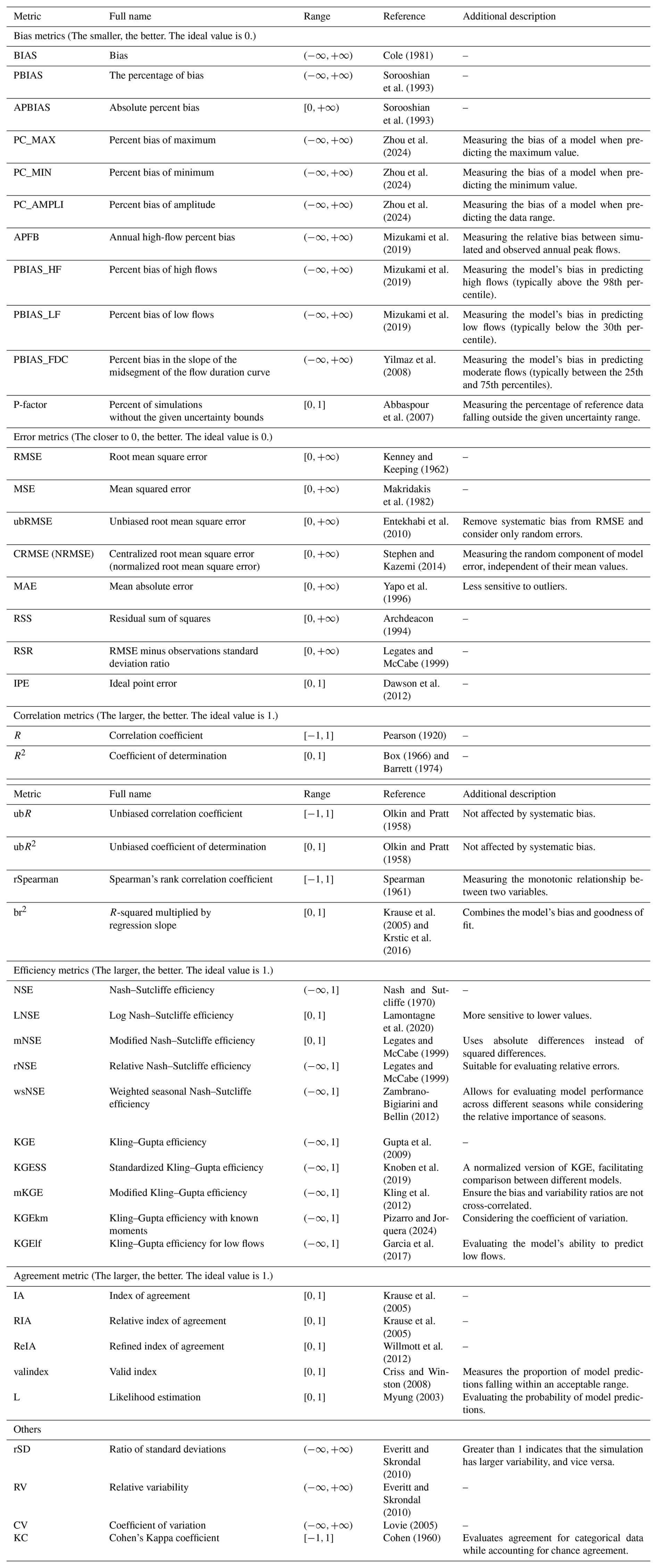
OpenBench uses a variety of metrics to evaluate LSM performance thoroughly (Table 2). This approach offers different viewpoints on model behavior, detailed comprehension of model strengths and weaknesses, versatile comparison abilities for both individual and inter-model assessments, and efficient implementation using Xarray and Dask software for handling large datasets. The system incorporates various categories of metrics to capture different aspects of model performance. For example, bias metrics, such as percent bias (PBIAS) and absolute percent bias (APBIAS), measure systematic over- or under-estimation and bias magnitude, respectively. Error metrics, including the root mean square error (RMSE), unbiased root mean square error (ubRMSE), centralized root mean square error (CRMSE), and mean absolute error (MAE), provide different perspectives on the magnitude and nature of model errors. Efficiency metrics like the Nash–Sutcliffe efficiency (NSE) and Kling–Gupta efficiency (KGE) evaluate model performance relative to baselines and combine multiple aspects of the model-data agreement. Correlation metrics, including the Pearson correlation coefficient (R) and coefficient of determination (R²), quantify the strength and direction of linear relationships between model outputs and observations. The index of agreement (IA) provides a more comprehensive assessment of magnitude and phase agreement. Variability metrics such as the ratio of standard deviations (rSD) and specialized bias metrics for maximum (PC_MAX), minimum (PC_MIN), and amplitude (PC_AMPLI) values help identify whether models accurately capture the range of system variability and extreme conditions. For categorical data, the Cohen's Kappa coefficient (KC) evaluates agreement while accounting for chance. Variability metrics such as relative variability (RV) and the coefficient of variation (CV) help identify whether models accurately capture the range of system variability. Bias-corrected versions of several metrics focus on assessing agreement in variability patterns after removing mean biases. In summary, this comprehensive approach provides a robust foundation for quantitative LSM assessment, enabling a multi-faceted evaluation that captures various aspects of the model-observation agreement. By implementing this range of metrics, OpenBench offers a thorough and nuanced evaluation of LSMs, supporting scientific understanding and practical model improvement.

3.2 The scoring index

OpenBench implements a suite of normalized score indices developed in ILAMB (Collier et al., 2018; Arora et al., 2023), ranging from 0 to 1, with 1 indicating perfect agreement between the model and observations. ILAMB encompasses several key indices, each designed to evaluate specific aspects of model performance. The normalized bias score (nBiasScore) quantifies systematic errors in the model's predictions, normalized by observational variability. For a given variable v(t,x), where t represents time and x represents spatial coordinates, we first calculate the bias from the temporal means of both the reference ${\stackrel{\mathrm{‾}}{v}}_{\text{ref}}\left(x\right)$ and model ${\stackrel{\mathrm{‾}}{v}}_{\text{sim}}\left(x\right)$ data. To score the bias, we normalize it by the centralized root mean square (CRMS) of the reference data:

$$\begin{array}{}\text{(1)}& \text{CRMS}\left(x\right)=\sqrt{{\displaystyle \frac{{\int }_{t_{\mathrm{0}}}^{t_{\mathrm{f}}}\left(v_{\text{ref}}\right(t,x)-{\stackrel{\mathrm{‾}}{v}}_{\text{ref}}(x){)}^{\mathrm{2}}\mathrm{d}t}{t_{\mathrm{f}}-t_{\mathrm{0}}}}},\end{array}$$

where t₀ and t_f are the first and final time step, respectively. We then compute the bias as $\text{bias}\left(x\right)=v_{\text{ref}}(t,x)-v_{\text{sim}}(t,x)$. The relative error in the bias is then given as ${\mathit{\epsilon }}_{\text{bias}}\left(x\right)=\frac{\left|\text{bias}\left(x\right)\right|}{\text{CRMS}\left(x\right)}$. The bias score as a function of space is then computed as:

$$\begin{array}{}\text{(2)}& \text{nBiasScore}\left(x\right)=e^{-{\mathit{\epsilon }}_{\text{bias}}\left(x\right)}.\end{array}$$

This score effectively penalizes large biases relative to the natural variability of the system. To evaluate the model's ability to capture observational variability, we employ the normalized RMSE score (nRMSEScore). Similar to nBiasScore, we first calculate the centralized RMSE (CRMSE):

$$\begin{array}{}\text{(3)}& \text{CRMSE}\left(x\right)=\sqrt{{\displaystyle \frac{\begin{array}{c}{\int }_{t_{\mathrm{0}}}^{t_{\mathrm{f}}}\left(\left(v_{\text{sim}}\right(t,x)-{\stackrel{\mathrm{‾}}{v}}_{\text{sim}}(x)\right)\\ -{\left(v_{\text{ref}}(t,x)-{\stackrel{\mathrm{‾}}{v}}_{\text{ref}}\left(x\right))\right)}^{\mathrm{2}}\mathrm{d}t\end{array}}{t_{\mathrm{f}}-t_{\mathrm{0}}}}}.\end{array}$$

The relative error in bias is then given as ${\mathit{\epsilon }}_{\text{rmse}}\left(x\right)=\frac{\text{CRMSE}\left(x\right)}{\text{CRMS}\left(x\right)}$. The nRMSEScore as a function of space is then computed as:

$$\begin{array}{}\text{(4)}& \text{nRMSEScore}\left(x\right)=e^{-{\mathit{\epsilon }}_{\text{rmse}}\left(x\right)}.\end{array}$$

This metric is particularly sensitive to differences in variability patterns between model outputs and observations. For variables with strong seasonal patterns, the normalized phase score (nPhaseScore) assesses the model's ability to capture the timing of seasonal cycles, providing insight into the model's representation of temporal dynamics. The nPhaseScore is calculated as:

$$\begin{array}{}\text{(5)}& \text{nPhaseScore}\left(x\right)={\displaystyle \frac{\mathrm{1}}{\mathrm{2}}}\left[\mathrm{1}+\cos \left({\displaystyle \frac{\mathrm{2}\mathit{\pi }\mathit{\theta }\left(x\right)}{\text{nstep}}}\right)\right],\end{array}$$

where $\mathit{\theta }(x,\mathit{\lambda },\mathit{\varphi })$ is the time difference between modeled and observed maxima:

$$\begin{array}{}\text{(6)}& \mathit{\theta }\left(x\right)=\text{maxima}\left(c_{\text{sim}}\right(x,t\left)\right)-\text{maxima}\left(c_{\text{ref}}\right(x,t\left)\right).\end{array}$$

Here, c_sim and c_ref are the climatological mean cycles (i.e., the average seasonal patterns) of the model and reference data, computed by averaging each month or day across all years in the time series. “maxima”( ) identifies the timing (month for monthly data, day for daily data) when the peak value occurs in these average seasonal cycles at each spatial location x. The parameter nstep represents the number of time steps in a complete annual cycle (e.g., 12 for monthly data or 365 for daily data) and normalizes the phase difference to the annual cycle.

Interannual variability, a critical aspect of climate modeling, is evaluated using the normalized interannual variability score (nIavScore). nIavScore is given by first removing the annual cycle from both the reference and model:

$$\begin{array}{}\text{(7)}& {\text{iav}}_{\text{ii}}\left(x\right)=\sqrt{{\displaystyle \frac{{\int }_{t_{\mathrm{0}}}^{t_{\mathrm{f}}}\left(v_{\text{ii}}\right(t,x)-c_{\text{ii}}(t,x){)}^{\mathrm{2}}\mathrm{d}t}{t_{\mathrm{f}}-t_{\mathrm{0}}}}},\end{array}$$

where ii represents sim or ref. Then, the relative error is calculated as:

$$\begin{array}{}\text{(8)}& {\mathit{\epsilon }}_{\text{iav}}\left(x\right)={\displaystyle \frac{{\text{iav}}_{\text{sim}}\left(x\right)-{\text{iav}}_{\text{ref}}\left(x\right)}{{\text{iav}}_{\text{ref}}\left(x\right)}}.\end{array}$$

Similar to Eqs. (2) and (4), the nIavScore is given by

$$\begin{array}{}\text{(9)}& \text{nIavScore}\left(x\right)=e^{-{\mathit{\epsilon }}_{\text{iav}}\left(x\right)}.\end{array}$$

This score is crucial for assessing the model's performance in representing year-to-year variations driven by climate factors. The spatial score (nSpatialScore) evaluates how well the model captures the spatial distribution of a variable compared to observations by assessing both the spatial correlation and the relative variability across the domain. The nSpatialScore is calculated as:

$$\begin{array}{}\text{(10)}& \text{nSpatialScore}=\mathrm{2}(\mathrm{1}+R)/{\left(\mathit{\sigma }+{\displaystyle \frac{\mathrm{1}}{\mathit{\sigma }}}\right)}^{\mathrm{2}},\end{array}$$

where R is the spatial correlation coefficient between the model and reference period mean values and σ is the ratio of spatial standard deviations:

$$\begin{array}{}\text{(11)}& \mathit{\sigma }=\text{stdev}\left({\stackrel{\mathrm{‾}}{v}}_{\text{sim}}\left(x\right)\right)/\text{stdev}\left({\stackrel{\mathrm{‾}}{v}}_{\text{ref}}\left(x\right)\right).\end{array}$$

To provide an overall assessment of model performance, we calculate an overall score (OvScore) that combines these individual metrics. This composite score gives double weight to the nRMSEScore due to its importance in capturing both bias and variability aspects, which is consistent with ILAMB. The relative score (ReScore) is designed to compare performance across simulations by normalizing a model's overall score relative to the multi-simulation mean and standard deviation. Positive values indicate above-average performance, while negative values indicate below-average performance. Detailed information can be obtained from Collier et al. (2018) and Arora et al. (2023).

ILAMB and OpenBench exhibit two key differences in their scoring methodologies. The first distinction lies in their approach to calculating global mean scores. ILAMB applies mass weighting when evaluating variables that represent carbon or water mass/flux, such as gross primary production (GPP) or precipitation. This method can lead to global mean scores being disproportionately influenced by middle and low latitudes, as exemplified by the significant impact of GPP or precipitation in the Amazon. In contrast, OpenBench offers greater flexibility in its weighting methods. OpenBench supports multiple weighting options that users can select based on their requirements. Users can choose between a simple spatial integral for unweighted averaging, area weighting to account for varying grid cell sizes across latitudes, or mass weighting for mass/flux variables. This flexibility allows researchers to choose the best weighting method for their particular analysis. For example, when evaluating GPP, researchers might opt for mass weighting to align with ILAMB's methodology, or they could choose area weighting to ensure more balanced representation across latitudes. The choice of weighting method can significantly impact the final results, particularly when analyzing variables with strong spatial heterogeneity. The second major difference pertains to how these systems handle multiple reference datasets. ILAMB combines evaluation results from different reference datasets, assigning weights to each and combining them multiplicatively to produce a single final score that incorporates all datasets. OpenBench, on the other hand, provides users with multiple reference datasets and allows them to select one or more that they consider most accurate. It then reports scores separately for each chosen dataset without applying weights. This approach gives users more flexibility and transparency in interpreting results, allowing them to make informed decisions based on their knowledge of dataset quality and relevance to their specific research questions. These methodological differences reflect the distinct philosophies and goals of each system. ILAMB's approach emphasizes a comprehensive, weighted assessment that accounts for the relative importance of different regions and datasets. OpenBench prioritizes user choice and equal spatial representation in its scoring methodology, allowing for a more customizable and potentially more equitable evaluation process. Both approaches have their merits, and the choice between them may depend on the specific needs and preferences of the research community using these benchmarking tools. It is worth noting that, although we refer to OpenBench as a “benchmarking system” in accordance with community convention, the tool primarily functions as an evaluation and comparison framework rather than adhering to strict benchmarking with predetermined performance standards. This design choice affords users the flexibility to establish their own performance criteria while benefiting from standardized evaluation methodologies.

In summary, by combining multiple normalized scores that assess different aspects of model performance, we enable a nuanced understanding of model strengths and weaknesses. This approach not only supports the evaluation of individual models but also facilitates inter-model comparisons and the tracking of model improvements over time.

3.3 Datasets

OpenBench integrates a diverse array of benchmarking data spanning multiple variables, levels, and spatiotemporal resolutions. This approach ensures a thorough evaluation of modern high-resolution LSMs, which require increasingly detailed and accurate input data to capture complex land–atmosphere interactions.

The strength of OpenBench lies in its extensive collection of baseline datasets, categorized into five main groups: radiation and energy cycle, ecosystem and carbon cycle, hydrology cycle, parameters and atmospheric forcing, and human activity. These datasets are derived from five primary sources: field observations, satellite remote sensing, reanalysis data, machine learning, and model outputs. Each source offers unique advantages, contributing to a more comprehensive understanding of land surface processes. Field observations provide high-accuracy, ground-truth data essential for model validation and calibration. While often limited in spatial coverage, these datasets offer unparalleled accuracy and temporal resolution. Satellite remote sensing delivers extensive spatial coverage and consistent temporal sampling, which are crucial for monitoring large-scale land surface processes. Reanalysis data combine model simulations with observations to create consistent, gridded data products, particularly useful for long-term studies or filling observational gaps. Model outputs and machine learning, while not direct observations, provide estimates of variables that are challenging to measure directly.

The spatiotemporal scope of OpenBench's datasets is another critical feature. Many datasets span several decades, allowing for the evaluation of long-term trends and interannual variability. This extended temporal coverage enables assessing LSMs' performance over long historical periods. The resolution ranges from coarse (e.g., 0.5° for ILAMB datasets; Collier et al., 2018) to very fine (e.g., 500 m for MODIS-based products; Varquez et al., 2021), making it possible to evaluate LSMs across different spatial scales, from global assessments to regional or plot-scale studies.

A unique aspect of OpenBench is its inclusion of datasets focused on human impacts on land surface processes. This approach recognizes the growing importance of anthropogenic factors in shaping the Earth system. Datasets like AH4GUC (Varquez et al., 2021), which provides global anthropogenic heat flux data, and GDHY (Iizumi and Sakai, 2020), offering detailed information on global crop yields, enable the evaluation of urban heat island effects and agricultural impacts in LSMs.

OpenBench's inclusion of multiple datasets for each variable allows for a more robust evaluation of LSMs. This multi-dataset approach enables users to assess model performance against a range of reference data, providing a more comprehensive evaluation. For instance, in evaluating evapotranspiration, OpenBench includes datasets like GLEAM4.2a (Miralles et al., 2011), FLUXCOM (Jung et al., 2019), X-BASE (Nelson et al., 2024), Xu2024 (Xu et al., 2025), and ERA5-Land (Muñoz-Sabater et al., 2021), each with its own methodology and characteristics. Users can assess model performance across multiple variables simultaneously, identifying potential compensating errors or cross-variable inconsistencies that might be missed when evaluating single variables in isolation. This multi-dimensional approach provides a more complete picture of model performance and helps guide future model development efforts. Meanwhile, OpenBench's dataset collection is designed to be expandable and updatable, ensuring its relevance in the rapidly evolving field of Earth system science. As new datasets become available or existing datasets are updated, they can be seamlessly integrated into the OpenBench framework.

It is noted that while OpenBench integrates with a comprehensive collection of datasets, we cannot directly provide specific data due to copyright restrictions and licensing agreements. However, to ensure transparency and reproducibility, we have included relevant links to the original data sources in Tables S1–S5 in the Supplement. These links will guide users to the appropriate platforms to access the datasets following the respective terms and conditions set by the data providers. To demonstrate the functionality and structure of OpenBench, we have included a set of self-generated sample data. These sample data mimic the characteristics and format of the actual datasets, allowing users to familiarize themselves with the OpenBench framework and its capabilities without infringing on any copyright issues. We encourage users to utilize these sample datasets for initial testing and exploration of the OpenBench system and then proceed to acquire the complete datasets from the original sources for comprehensive model evaluations.

3.4 Supporting models

OpenBench has been designed to accommodate a diverse array of land surface models, facilitating comprehensive intercomparison and evaluation studies. This multi-model support is a key feature of OpenBench, enabling researchers to assess and compare the performance of various models across different land surface processes and variables. Currently, OpenBench supports various state-of-the-art land surface models, including multiple versions of the Common Land Model (CoLM2014 and CoLM2024) (Bai et al., 2024; Dai et al., 2003; Fan et al., 2024), the Community Land Model Version 5 (CLM5) (Lawrence et al., 2019), Noah-MP 5.0 (He et al., 2023), the Minimal Advanced Treatments of Surface Interaction and Runoff model (Version 2021) (Nitta et al., 2014), the Atmosphere–Vegetation Interaction Model (AVIM) (Li et al., 2002), the Global Land Data Assimilation System (GLDAS2) (Rodell et al., 2004), Today's Earth (TE) (https://www.eorc.jaxa.jp/water/index.html, last access: 8 July 2025), the Variable Infiltration Capacity (VIC) model (Hamman et al., 2018), and so on. OpenBench has expanded its capabilities to support Lambert conformal projection outputs from regional climate models such as the climate extension of the Weather Research and Forecasting model (CWRF) (Liang et al., 2012) and the Weather Research and Forecasting (WRF) model (Lo et al., 2008).

Furthermore, OpenBench supports CMIP-style series outputs, such as CMIP-style simulation, e.g., LS3MIP (Van Den Hurk et al., 2016) and ISIMIP (Wartenburger et al., 2018), allowing for seamless integration of global climate model data into the evaluation framework. Each supported model is integrated into the system through a dedicated namelist file that maps the model's output variables to standardized variables used within OpenBench. This approach ensures consistent comparison and evaluation across different models, regardless of their native output format or projection.

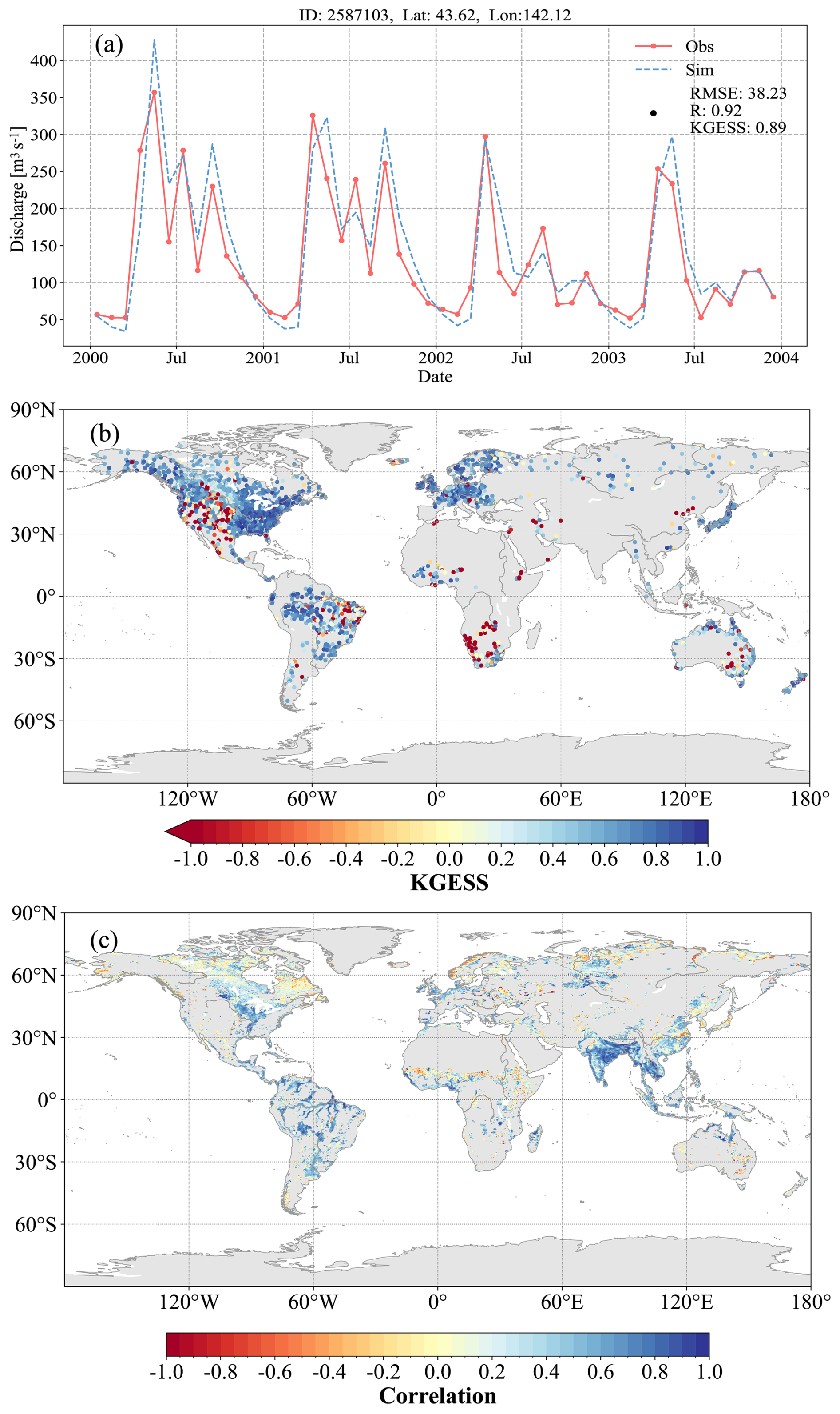
Figure 2 Example of river discharge evaluation: (a) simulated and observed discharge hydrographs for an example station; (b) global maps of KGESS values for the simulated discharge dataset; and (c) global maps of R values for the simulated inundation dataset.

3.5 Case studies

To illustrate the analytical capabilities of our evaluation system, we present comprehensive case studies focusing on two critical aspects of hydrological modeling: river discharge evaluation and inundation fraction assessment. These analyses were conducted using simulations from the CaMa-Flood Version 4.22 model (Yamazaki et al., 2013), driven by 0.25° remapped daily runoff data from the Global Reach-level Flood Reanalysis (GRFR) (Yang et al., 2021). The evaluation was performed globally with 0.25° spatial resolution, utilizing observational data from the Global Runoff Data Centre (GRDC) for discharge validation and the Global Inundation Extent from Multi-Satellites (GIEMS) (Prigent et al., 2020) for inundation fraction assessment. Our analysis demonstrates the system's versatility in conducting site-specific and global-scale evaluations. Figure 2a presents a detailed comparison of simulated and observed discharge hydrographs for a representative station. This station-level analysis reveals the model's strong performance in capturing both the magnitude and temporal variability of discharge patterns. The close alignment between simulated and observed values indicates robust model performance at the local scale. Figure 2b illustrates the spatial distribution of KGESS values for simulated discharge across the globe. The analysis reveals distinct regional patterns in model performance. The model demonstrates particularly strong capabilities in simulating discharge across wet regions, including the Amazon basin, Japan, and the Eastern United States. However, performance metrics indicate lower accuracy in the Western United States, Central Australia, and Southern Africa. These regional variations can be attributed to several factors, including the influence of human activities, uncertainties in precipitation datasets, and limitations in model parameterization schemes (Wei et al., 2020). The impact of human activities on model performance is particularly evident in regions like the Western United States, where discharge patterns are significantly modified by dam operations (Hanazaki et al., 2022). This finding underscores the importance of incorporating human water management practices in regions with intensive anthropogenic influence to achieve reliable simulation results. Figure 2c presents global patterns of correlation coefficients for the simulated inundation fraction. The results indicate strong model performance in low-latitude regions, particularly in the Amazon basin and South Asia. However, significant discrepancies emerge in high-latitude areas (above 60° N). This spatial pattern of model performance highlights the need for improved representation of snow-related processes and precipitation phase partitioning in these regions (Jennings et al., 2018).

Figure 3 An example of a scores heat map for GPP classified by IGBP land cover.

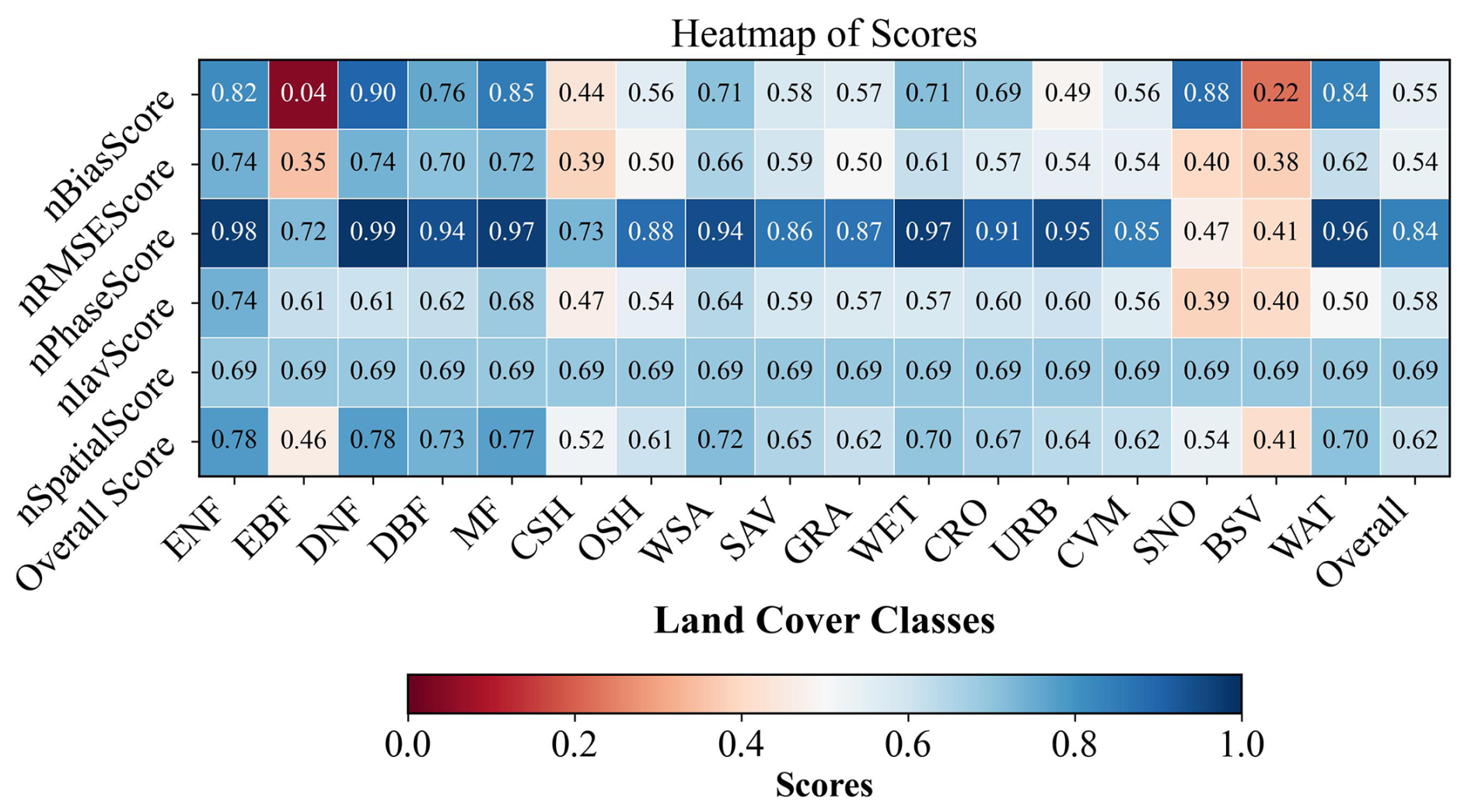
OpenBench implements automated grouping of metrics and scores according to both IGBP and PFT classifications to provide a comprehensive evaluation of model performance across diverse ecological zones. Figure 3 presents a detailed heat map visualization of performance indices categorized by IGBP land cover type, based on CoLM2024 simulations evaluated against X-BASE reference data (Nelson et al., 2024) for 2002–2003. The analysis incorporates six fundamental performance scores developed within the ILAMB framework, as detailed in Sect. 3.2. The visualization reveals several significant patterns in model performance across different ecosystems. The overall nPhaseScore of 0.84 demonstrates the model's robust capability in capturing seasonal variations across all biomes. Particularly noteworthy is the model's exceptional performance in forest ecosystems, where evergreen needleleaf forests (ENFs), deciduous needleleaf forests (DNFs), and mixed forests (MFs) exhibit consistently high nPhaseScore. These results indicate the model's sophisticated ability to simulate the complex dynamics of multi-layered forest ecosystems. However, the analysis also identifies specific challenges in certain environmental contexts. The model's performance notably decreases in extreme environments, with lower scores across multiple metrics for snow and ice (SNO) and barren or sparsely vegetated (BSV) regions. It is important to highlight that the GPP values found in the SNO and BSV classes could stem from spatial or temporal misalignments between the IGBP land cover classification and GPP datasets. Specifically, pixels identified as non-vegetated during the land cover survey might have had vegetation during the GPP measurement periods, or mixed pixels may consist of minor vegetated fractions within primarily barren regions. Additionally, evergreen broadleaf forests (EBFs) show a particularly low nBiasScore, reflecting substantial magnitude discrepancies between simulated and observed values. This finding underscores the persistent challenges in accurately modeling these data-sparse, highly dynamic ecosystems. These insights have important implications for model application across different research contexts. Researchers focusing on temperate and boreal forest ecosystems can proceed with high confidence in the model's capabilities. However, studies targeting arid regions, snow-covered areas, or tropical rainforests should incorporate additional validation steps and exercise greater caution in interpreting results. This systematic evaluation across biomes thus provides essential guidance for appropriate model application in diverse ecological settings.

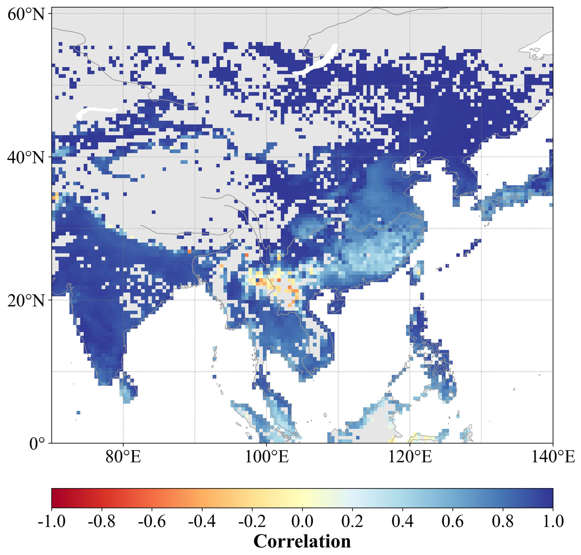
Figure 4 Pearson's correlation coefficient between the CoLM2024 simulation and AH4GUC generation for urban anthropogenic heat flux over Southeast Asia.

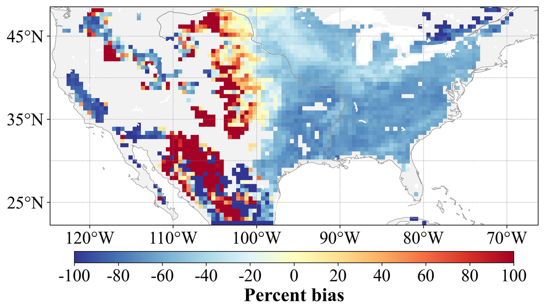
Figure 5 Percentage bias between CoLM2024 simulated and GDHY generated crop yield of corn for the United States.

Figure 4 demonstrates OpenBench's capability to evaluate anthropogenic influences on urban thermal environments through a detailed comparison of CoLM2024 simulations with AH4GUC observational data for Southeast Asia. The analysis reveals generally strong agreement between simulated and observed anthropogenic heat flux patterns across most regions. However, notable discrepancies emerge in specific areas, particularly the corridor extending from central China to northern Vietnam and regions near Laos, where negative correlations indicate potential systematic biases in model representation. While the exact mechanisms driving these regional differences are still being investigated, these results demonstrate OpenBench's ability to identify spatial patterns of model-observation disagreement that require further exploration. The system's evaluation capabilities extend beyond thermal processes to encompass multiple aspects of human–environment interactions. Through a comprehensive assessment of variables, including latent heat, albedo, and surface temperature changes, OpenBench provides valuable insights into the complex relationships between anthropogenic activities and land surface processes, guiding improvements in their model representation.

Figure 5 presents a detailed analysis of agricultural modeling capabilities, comparing CoLM2024 simulated corn yields with GDHY-generated observational data across the United States. The analysis reveals distinct regional patterns in model performance: approximately 20 % yield underestimation in the Western United States, significant overestimation in central regions, and notable underestimation in eastern areas. These spatial patterns of bias may stem from multiple sources, including uncertainties in the GDHY observational dataset and the CoLM2024 model structure. Particularly noteworthy are the substantial differences in planted area and crop distribution between the two datasets, indicating fundamental challenges in representing agricultural systems within current modeling frameworks. These findings underscore the significant opportunities for advancement in both modeling and observational approaches to crop yield estimation. Future research efforts should focus on reducing uncertainties in simulation and observational datasets while improving the representation of agricultural processes in land surface models.

In summary, these case studies demonstrate the comprehensive analytical capabilities of our evaluation system. Through its ability to conduct detailed analyses across multiple spatial scales and variables, OpenBench provides researchers with powerful tools for assessing model performance and identifying specific areas for improvement. This multi-scale, multi-variable approach supports theoretical understanding and practical application of land surface models, ultimately contributing to enhanced representation of Earth system processes.

4 Comparisons

4.1 Overview

OpenBench offers a comprehensive suite of comparison capabilities designed to facilitate a thorough evaluation of model performance across diverse scenarios, land cover types, and temporal scales. The system incorporates several key functionalities that enable sophisticated analysis while maintaining user accessibility and scientific rigor.

The framework's evaluation architecture encompasses multiple complementary approaches to model assessment. At its foundation, ecosystem-based comparisons allow researchers to evaluate performance across different IGBP and PFT land cover classifications, providing crucial insights into model behavior within specific ecological contexts. This capability is enhanced by multi-metric visualization tools, including heat maps, Taylor diagrams, and target diagrams, which offer intuitive yet comprehensive overviews of model capabilities by simultaneously displaying multiple statistical metrics for model-observation comparisons. To support detailed analysis of model behavior, OpenBench implements advanced distribution and pattern analysis tools. These include kernel density estimation plots and parallel coordinate plots, which facilitate the comparison of metric distributions across models and enable the identification of patterns in multivariate performance data. The system's temporal performance evaluation capabilities, implemented through seasonal portrait plots, provide detailed insights into variations in model accuracy across different seasonal cycles. Statistical analysis within OpenBench is supported by robust summary tools, including box and whisker plots that offer concise yet comprehensive overviews of model performance across different metrics and scenarios. This statistical framework ensures that comparisons remain objective and scientifically sound while presenting results in an accessible format for interpretation.

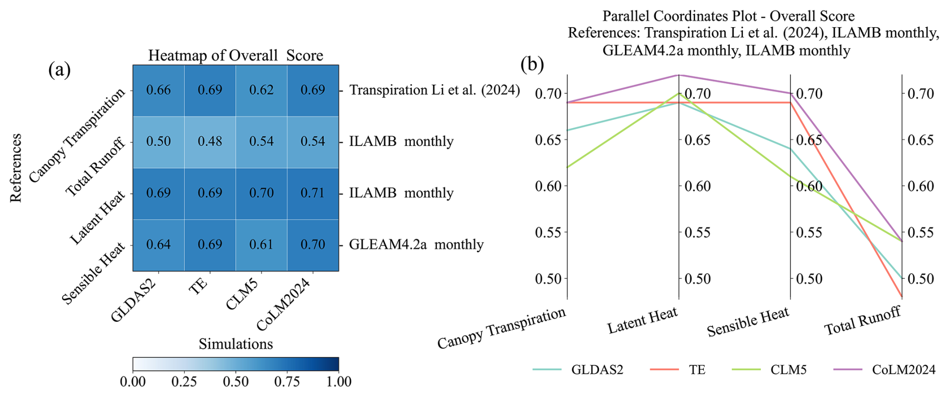
Figure 6 Overall score comparisons of sensible heat, latent heat, total runoff, and canopy transpiration using (a) heat map and (b) parallel coordinates approaches for GLDAS2, TE, CLM5, and CoLM2024.

The implementation of multiple model comparisons follows a systematic and efficient approach. The process begins with the standardization of model outputs through a sophisticated data processing pipeline, capable of handling various input formats and temporal/spatial resolutions. The comparison processing module orchestrates this analysis through support for multiple comparison methods, with parallel processing capabilities implemented via the Joblib library to ensure computational efficiency. Evaluation items and reference sources systematically organize results from the comparison process within a structured output directory. The system automatically generates comparison artifacts, including metrics and score files, which form the basis for comprehensive visualization and analysis. This structured approach ensures that adding new models to the comparison framework requires minimal effort, typically involving only the update of the simulation namelist with new model information and data sources. This integrated approach to model comparison and evaluation provides researchers with powerful tools for understanding model behavior while maintaining the flexibility needed to address diverse research questions in land surface science. The system's design philosophy emphasizes scientific rigor and practical utility, ensuring that comparative analyses can be conducted efficiently while maintaining the highest standards of scientific validity.

4.2 Case studies

To demonstrate the comprehensive capability of our evaluation system, we present several case studies to demonstrate the ability of the evaluation system to compare between models, compare between different parameterized schemes, and compare between CMIP-style datasets. It's important to note that our primary goal is to showcase the evaluation system's functionality rather than to make definitive judgments about any particular model's performance. These case studies are practical examples of the system's versatility and analytical power.

4.2.1 Comparison of multiple models

To demonstrate the analytical capabilities of OpenBench for multiple models, we conducted a comparative analysis of four state-of-the-art land surface models: GLDAS2, TE, CLM5, and CoLM2024. The evaluation period spanned from 2002 to 2006, utilizing a monthly temporal resolution. Multiple reference datasets were incorporated, including Li et al. (2024) for canopy transpiration, the FLUXCOM dataset (from ILAMB) and GLEAM4.2a for surface heat fluxes, and LORA (from ILAMB) for total runoff assessment (Hobeichi et al., 2019).

Figure 6 illustrates the comparative analysis through two complementary visualization approaches: a heat map and a parallel coordinates plot. The heat map (left panel) provides an intuitive visualization of relative model performance across different variables, while the parallel coordinates plot (right panel) reveals intricate relationships between various performance metrics. This dual visualization strategy enables researchers to quickly identify patterns and trade-offs in model performance across multiple variables simultaneously. The analysis reveals that under current configurations, CoLM2024 and TE achieve the highest score for canopy transpiration, while CLM5 and CoLM2024 show the highest score for total runoff. CoLM2024 maintains a relatively higher score for the other variables.

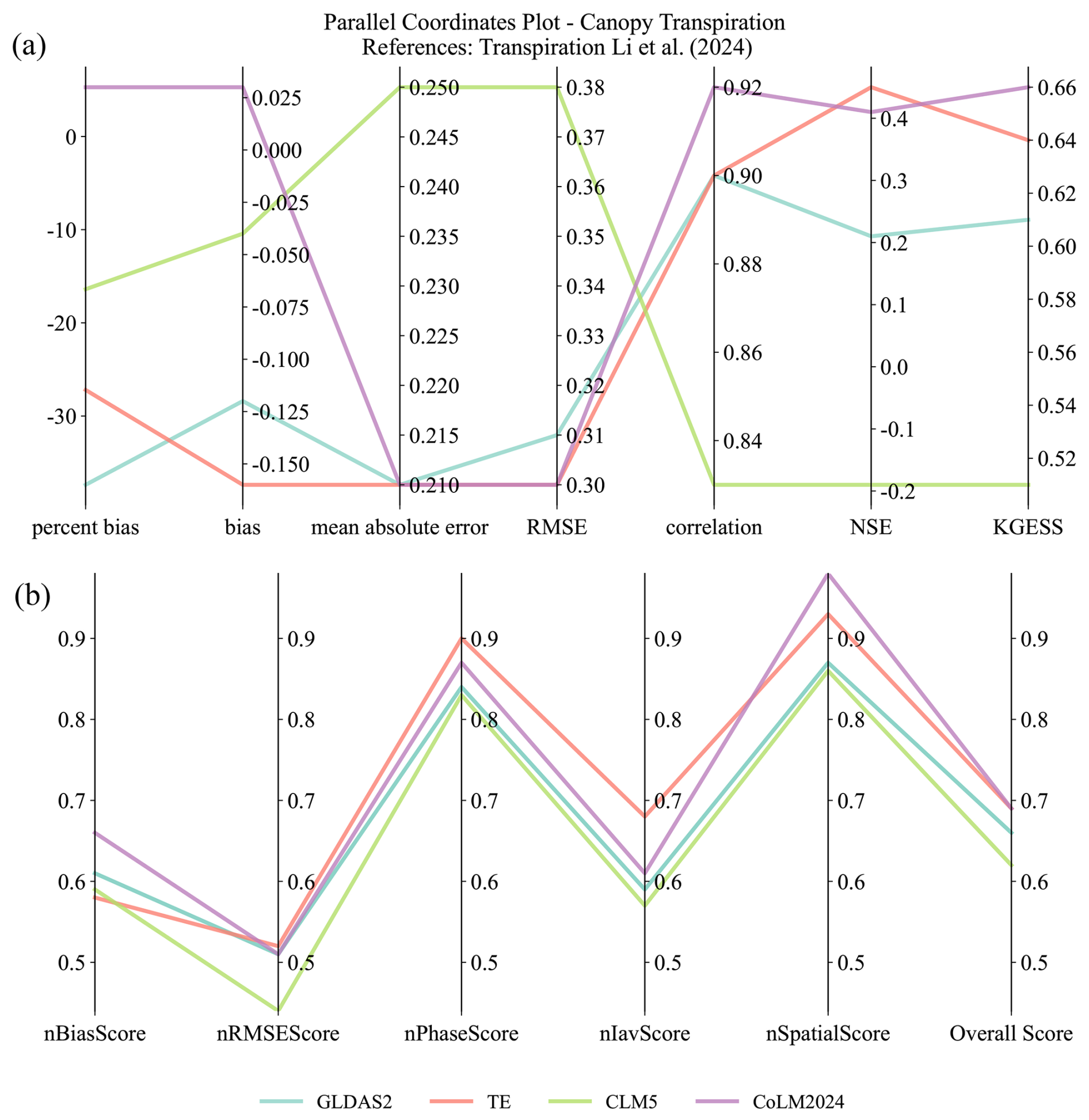
Figure 7 Evaluation of canopy transpiration using various (a) metrics and (b) score indexes for GLDAS2, TE, CLM5, and CoLM2024.

For detailed variable-specific analysis, Fig. 7 presents an in-depth examination of canopy transpiration across all models, utilizing both conventional metrics (Fig. 7a) and normalized scores (Fig. 7b). The metrics analysis reveals that CoLM2024 exhibits a tendency to overestimate canopy transpiration, while other models show varying degrees of underestimation, as indicated by the percent bias metric. Furthermore, CoLM2024 achieves optimal performance regarding RMSE minimization, correlation maximization, and KGESS optimization. TE demonstrates particularly strong performance in NSE and ranks second in KGESS. Regarding scoring indices, TE excels in nRMSEScore, nPhaseScore, and nIavScore, whereas CoLM2024 achieves the highest nBiasScore.

This comprehensive comparative analysis not only highlights the relative strengths and weaknesses of each model but also offers valuable insights into their simulation capabilities regarding various aspects of land surface processes. Such a detailed evaluation helps identify areas where models excel or need further refinement, effectively guiding future development efforts.

4.2.2 Multiple parameterizations and multiple references

To evaluate the versatility of OpenBench in analyzing model parameterization schemes, we conducted a comprehensive assessment of different runoff generation parameterizations within the CoLM2024 model framework. The analysis focused on daily discharge simulations at 0.1° resolution from 1985 to 1999, comparing three distinct parameterization approaches: SIMTOP, Xinanjiang, and SimpleVIC. These simulations were evaluated against observational data from GRDC.

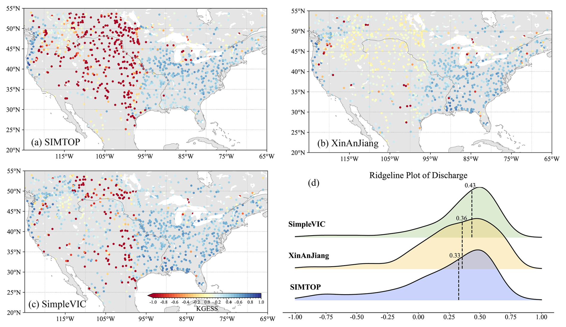
Figure 8 Comparison of daily discharge simulated from different parameterizations of the CoLM2024 model's runoff generation scheme with GRDC observations using the KGESS metric.

Figure 8 presents a spatial analysis of model performance using the KGESS metric across the continental United States. The station-based visualization (Fig. 8a–c) reveals distinct spatial patterns in model performance for each parameterization scheme. The SimpleVIC parameterization demonstrates superior performance across most regions, particularly in areas with complex hydrological processes. In contrast, the Xinanjiang scheme exhibits notable strengths in simulating discharge patterns within arid and semi-arid regions, suggesting its particular effectiveness in water-limited environments.

To further elucidate the statistical characteristics of these parameterizations, we employed a ridgeline plot analysis (Fig. 8d). This visualization technique effectively captures the distribution of performance metrics across different schemes, with the dashed lines and accompanying numbers indicating median values for each parameterization. The analysis confirms that the SimpleVIC parameterization achieves the highest overall performance metrics, though each scheme shows specific regional strengths.

OpenBench's capability to handle multiple reference datasets is demonstrated through a detailed evaluation of latent heat simulations. Figure 9 illustrates this multi-reference analysis framework, comparing CoLM2024 simulations against four distinct reference sources: satellite-derived products (CLASS), machine learning outputs (FLUXCOM), in situ measurements (PLUMBER2) (Ukkola et al., 2022), and reanalysis data (ERA5Land). This comparison was conducted at a monthly temporal resolution and 0.5° spatial resolution for the period 2002–2006. The resulting heat map visualization reveals strong model–data agreement across all reference datasets, with correlation coefficients consistently exceeding 0.90.

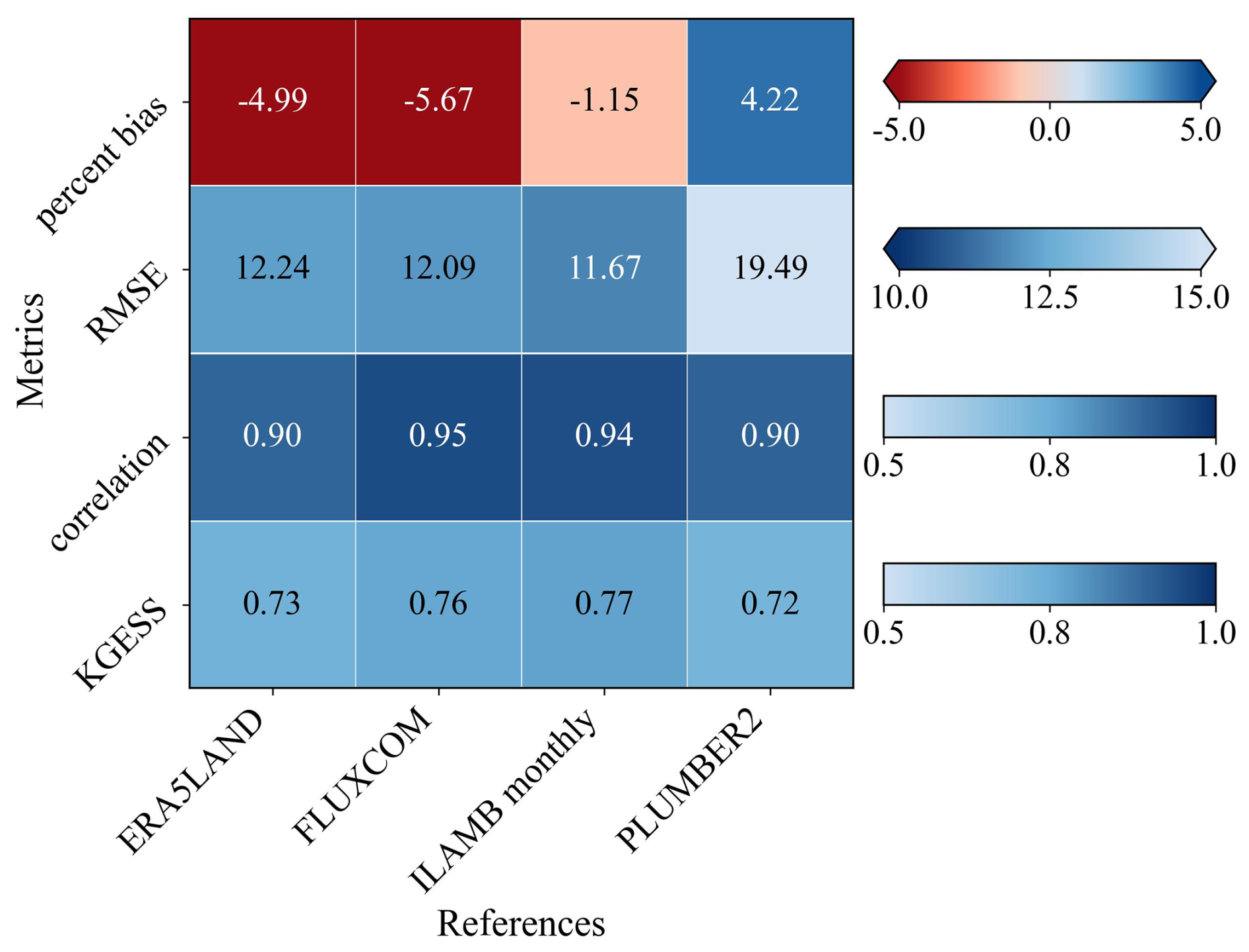
Figure 9 Evaluation of latent heat flux simulated by CoLM2024 using various metrics with different reference datasets.

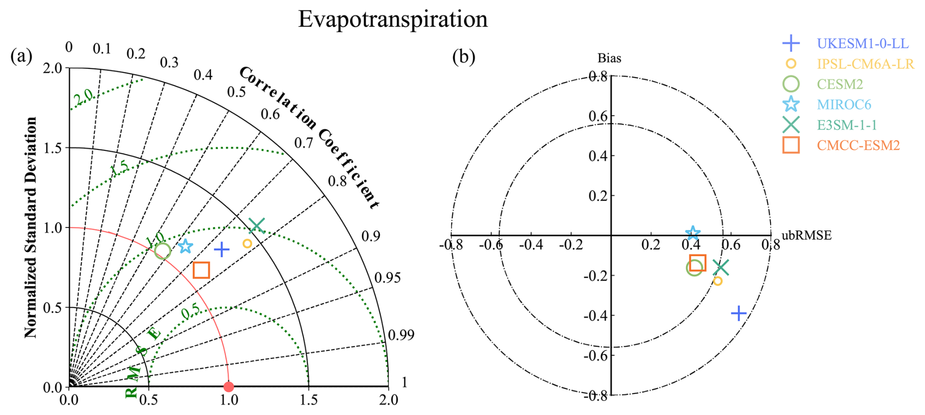
Figure 10 The Taylor (a) and target (b) diagram for comparing evapotranspiration among the six models in LS3MIP.

This comprehensive evaluation approach validates the model's performance against multiple independent data sources and provides insights into the structural uncertainties inherent in different observational datasets. Such multi-reference validation is particularly valuable for variables where direct measurements are sparse and each observational approach has its own uncertainties and biases. The consistently high correlation values across different reference datasets enhance confidence in the model's ability to capture fundamental physical processes while also highlighting areas where uncertainties in observational data may impact validation efforts.

4.2.3 CMIP styles comparison

OpenBench's evaluation framework incorporates robust capabilities for analyzing CMIP-style datasets, with particular emphasis on experimental outputs from initiatives such as ISIMIP and LS3MIP. The system's architecture includes specialized data processing modules designed to handle the standardized conventions of CMIP outputs, including variable naming conventions, temporal frequencies, and grid structures, ensuring seamless integration with the evaluation framework.

Figure 10 demonstrates this capability through a comprehensive analysis of evapotranspiration simulations from the LS3MIP experiment. The analysis employs both Taylor and target diagrams to provide complementary perspectives on model performance. The Taylor diagram (Fig. 10a) effectively visualizes the relationship between correlation coefficients, normalized standard deviations, and centralized root mean square errors. This multi-metric representation enables immediate identification of models that achieve optimal balance across these key performance indicators. The target diagram (Fig. 10b) supplements this analysis by providing additional insight into bias components and pattern variations, with distinct symbols differentiating between the various LS3MIP simulations.

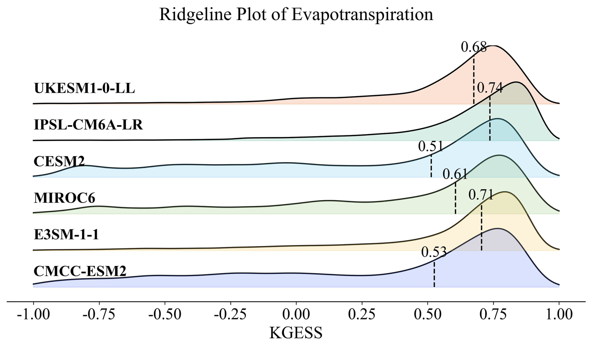
Figure 11 Ridgeline plot comparing evapotranspiration for the six models in the LS3MIP Land-hist experiment.

To further elucidate the performance distribution across different models, Fig. 11 presents a ridgeline plot analysis of the KGESS metric. This visualization technique reveals the full spectrum of model performance, highlighting both central tendencies and variations in simulation quality. The analysis demonstrates that while certain models consistently achieve higher performance metrics, considerable variation in simulation quality exists across the ensemble. This variation provides valuable insights into the structural uncertainties inherent in current land surface modeling approaches. The integration of CMIP-style evaluation capabilities within OpenBench serves multiple critical functions in the broader context of Earth system modeling. First, it enables systematic assessment of land surface processes within coupled climate models, providing essential feedback for model development and improvement. Second, it facilitates direct comparisons between offline land surface model simulations and their behavior within coupled frameworks, helping to identify potential interactions and feedback that may affect model performance. Finally, this capability supports comprehensive model intercomparison studies, contributing to our understanding of model uncertainties and their implications for future climate projections.

This robust framework for evaluating CMIP-style outputs positions OpenBench as a valuable tool for both model development and climate change research. By providing standardized, comprehensive evaluation metrics for these complex datasets, OpenBench supports the ongoing effort to improve our understanding and prediction of land surface processes in the context of global climate change.

5 Extensibility and customization

OpenBench is engineered with extensibility and customization as core design principles, enabling the system to evolve alongside the rapidly advancing field of land surface science. This flexible architecture accommodates the integration of new models, variables, datasets, measurement units, evaluation metrics, and scoring systems while maintaining operational consistency and scientific rigor. The system's modular design facilitates seamless incorporation of new reference datasets through a streamlined configuration process. Researchers can integrate additional observational or reanalysis data by creating appropriate entries in the reference configuration file, specifying dataset locations and characteristics. This process involves defining dataset properties, including directory structures, temporal and spatial resolutions, and variable-specific parameters. For datasets with unique characteristics, users can develop custom processing scripts that integrate smoothly with the existing evaluation framework.

Variable integration follows a similarly structured approach. Adding new variables requires coordinated updates to both reference and simulation configuration files, alongside corresponding dataset configurations that define variable properties. This process may include the development of specialized evaluation metrics and visualization components to effectively represent and analyze the new variables within the system's analytical framework. The integration of new land surface models demonstrates OpenBench's architectural flexibility. Users can incorporate additional models by creating model-specific namelist files that establish straightforward mappings between model outputs and OpenBench's standardized variables. This integration is supported by updates to the simulation configuration and, where necessary, the development of custom variable filtering scripts to handle model-specific output characteristics. OpenBench's unit conversion system exemplifies its sophisticated approach to extensibility. The unit processing module employs a flexible design that readily accommodates new measurement units for existing and new variables. Users can implement additional unit conversions by creating methods within the designated class, following established naming conventions. The system's dynamic method calling architecture ensures that new unit conversions integrate seamlessly into the evaluation workflow without requiring modifications to other system components. The system's evaluation framework maintains equal flexibility in incorporating new metrics and scoring methodologies. Users can implement additional evaluation metrics by creating new methods within the metrics class, properly handling missing data, and maintaining comprehensive documentation. Similarly, new scoring systems can be integrated into the scores class within Mod_Scores.py, with appropriate attention to normalization procedures and interpretation guidelines.

This comprehensive approach to extensibility guarantees that OpenBench stays at the forefront of land surface model evaluation capabilities. As new scientific questions emerge, new models are developed, and new observational datasets become available, the system can readily adapt to incorporate these advances. This flexibility is essential for maintaining a state-of-the-art evaluation framework that effectively serves the evolving needs of the land surface modeling community while ensuring consistent, high-quality analysis across various applications and research contexts.

6 Conclusions

Our newly developed OpenBench represents a significant advancement in land surface model evaluation methodology, addressing critical gaps in existing evaluation frameworks while introducing innovative capabilities for comprehensive model assessment. By integrating high-resolution benchmark datasets, sophisticated evaluation metrics, and efficient data-handling mechanisms, OpenBench provides users with a powerful tool for enhancing the understanding and performance of land surface models. The system's key strengths lie in several areas. First, its ability to handle diverse data types and formats, from station-based measurements to gridded products, enables comprehensive evaluation across multiple spatial and temporal scales. Second, incorporating human activity impacts into the evaluation framework fills a crucial gap in current assessment tools, allowing for a more realistic evaluation of model performance in anthropogenically modified landscapes. Third, the system's robust computational architecture, built on efficient parallel processing and standardized data-handling protocols, ensures scalability and reliability in processing large-scale datasets. The case studies presented demonstrate OpenBench's practical utility across various applications. The system has proven effective in identifying model strengths and areas requiring improvement, from evaluating hydrological processes and urban heat fluxes to assessing agricultural modeling capabilities. The multi-reference approach to model evaluation provides particularly valuable insights, helping distinguish between model deficiencies and observational uncertainties. OpenBench's extensible architecture ensures its continued relevance as the field evolves. The system's ability to incorporate new models, variables, datasets, and evaluation metrics allows it to adapt to emerging research needs and technological advances. This flexibility, combined with its comprehensive evaluation capabilities, positions OpenBench as a valuable resource for both model development and operational applications. Looking forward, OpenBench's role in advancing land surface modeling extends beyond technical evaluation. By providing standardized and reproducible evaluation methods, OpenBench facilitates more effective collaboration within the modeling community and supports more informed decision-making in environmental management. As we face increasing environmental challenges and seek to improve our understanding of Earth system processes, tools like OpenBench will be crucial in developing more accurate and reliable land surface models.