BIOPERIANT12: a mesoscale-resolving coupled physics–biogeochemical model for the Southern Ocean

We present BIOPERIANT12, a regional $\mathrm{1}/\mathrm{12}$° ocean–ice–biogeochemical model configuration of the Southern Ocean (SO) based on the Nucleus for European Modelling of the Ocean platform. It is designed to investigate mean state, seasonal cycle, and upper ocean (< 500 m) dynamics, with a particular focus on processes influencing carbon, heat exchange, biogeochemical mechanisms, and the assumptions underlying physical–biogeochemical model parameterisations within the SO. Over the analysis period 2000–2009, the model demonstrates a stable and realistic upper ocean mean state compared to observation-based products. We use ocean biomes to delineate the major subregions and evaluate the biogeochemical properties of the model, including surface chlorophyll and partial pressure of carbon dioxide. BIOPERIANT12 captures key spatial and temporal features of SO biogeochemistry (BGC), though it tends to overestimate biological biomass and underrepresents high-frequency variability. The model shows skill in reproducing large-scale patterns and seasonal cycles across biomes, offering insights into regional dynamics that are often obscured in coarser models. Despite its limitations, BIOPERIANT12 provides a valuable high-resolution framework for process studies, model–data intercomparisons, and future investigations into mesoscale influences on carbon and heat dynamics. It offers a useful tool for addressing long-standing uncertainties in air–sea exchange and ecosystem variability in the SO.

1 Introduction

The Southern Ocean (SO) is a key region in the global carbon cycle, serving as a major sink for both carbon dioxide (CO₂) and heat. It accounts for nearly 40 % of the annual mean oceanic CO₂ uptake and 75 % of the global excess heat (Frölicher et al., 2015; Gruber et al., 2023). However, the SO remains a challenging region to both observe and simulate. The recognised sparsity of observations in this dynamic, remote area has been addressed through expanded sampling efforts since the 2000s (Williams et al., 2018; Meredith et al., 2013; Swart et al., 2012). Owing to improvements in sampling technology, data are now being collected at unprecedented temporal and spatial resolutions. Despite this progress, the data remain weakly constrained and seasonally biased. Model–data comparisons have thus underscored the need to improve the representation of CO₂ and heat fluxes in ocean models and Earth system models (ESMs) used for future climate projections (Rintoul, 2018).

Model ocean dynamics are fundamental to accurately reproducing CO₂ and heat fluxes in the SO, particularly due to the prevalent mesoscale eddy field driven by the Antarctic Circumpolar Current (ACC) and its associated strong mesoscale kinetic energy and baroclinic instabilities (Daniault and Ménard, 1985; Smith et al., 2023). Mesoscale dynamics account for a substantial portion of both annual and seasonal variance in mixed layer depth (MLD) (Whitt et al., 2019; Gaube et al., 2019), thereby influencing global circulation through water mass transformation and SO overturning circulation via eddy compensation and ocean–wind interactions (Abernathey et al., 2016; Munday et al., 2014). Subsequently, enhanced advection and mixing by mesoscale (and submesoscale) processes affect local biogeochemistry (BGC) through the supply of limiting nutrients to the euphotic layer (Frenger et al., 2015; Nicholson et al., 2019; Uchida et al., 2019) and by modifying light availability through stratification caused by “eddy slumping” during spring (Lévy et al., 1998, 1999; Marshall et al., 2002; Lévy et al., 2010; Mahadevan et al., 2012).

Within the framework of the seasonal cycle, arguably the dominant mode of variability in physical–biogeochemical properties of the SO (Lenton et al., 2013; Thomalla et al., 2011; Mongwe et al., 2018; Gregor et al., 2019; Rodgers et al., 2023), ocean models continue to show inadequate representation of SO dynamics (Chassignet et al., 2020; Treguier et al., 2023). This leads to large model biases in ESMs and a wide inter-model spread in previous generations of the Climate Model Intercomparison Project (CMIP). For example, models show divergent seasonal cycles in air–sea CO₂ flux (FCO₂), (Anav et al., 2013; Lenton et al., 2013; Kessler and Tjiputra, 2016; Mongwe et al., 2016, 2018), sea ice extent and trends (Meijers, 2014; Beadling et al., 2020), MLD (Sallée et al., 2013; Treguier et al., 2023), water mass properties (Downes et al., 2015; Beadling et al., 2020), dissolved iron concentrations (Tagliabue et al., 2016), and phytoplankton phenology (Thomalla et al., 2011, 2023; Hague and Vichi, 2018).

The representation of mesoscale dynamics in ocean models is therefore a critical step toward improving the simulation of CO₂ and heat fluxes. Coupled physics–BGC simulations, in both global (Rohr et al., 2020) and regional models (Song et al., 2018; Uchida et al., 2019, 2020), demonstrate that model resolution strongly influences biological responses in the SO. These effects arise through more refined representations of both physical and biogeochemical mechanisms, particularly in the structure and timing of seasonal cycles. However, the ability to resolve such processes is limited by computational costs, especially in models that include BGC components. BGC can add substantially to the overall cost which increases with the number of BGC tracers that must be advected and the complexity of numerical schemes employed (Lévy et al., 2012). For long-running coupled models designed to address climate-scale questions, lower resolutions are thus often used. This choice contributes to uncertainties in simulating carbon and heat exchange (Hewitt et al., 2020; Beadling et al., 2020). Despite gains in computational power, demonstrated by the shift from CMIP5 models with horizontal resolutions coarser than 1° to CMIP6 models of up to 0.25°, most ESMs still do not explicitly resolve mesoscale processes in the SO (Hewitt et al., 2020; Haarsma et al., 2016).

To balance computational constraints, model configurations, especially those incorporating BGC, must make trade-offs in spatial and temporal resolution, run duration, and model complexity. For simulations focused on SO CO₂ and heat fluxes, resolution is critical: it defines the spatial scales over which ocean dynamics operate to distribute BGC tracers, and significantly contributes to model–observation discrepancies. For example, mesoscale modulation of the MLD affects light and iron availability at the surface, which in turn influences phytoplankton growth and the strength of the biological carbon pump (Song et al., 2018). In addition, low-resolution models are more prone to cumulative errors in BGC fields, such as nutrient and iron pools, which can propagate and amplify over time (Séférian et al., 2013).

In this paper, we present our regional SO model configuration of a laterally unconstrained ACC with resolved eddies and a prescribed atmosphere. BIOPERIANT12 is a regional, circumpolar, mesoscale-resolving (1/12°), contemporary ocean–ice–BGC model configuration using NEMO–PISCES. The PISCES biogeochemical model simulates 24 evolving prognostic tracers for carbon and nutrients cycles, as well as marine productivity, with two phytoplankton groups (nanophytoplankton and diatoms) and two zooplankton groups (microzooplankton and mesozooplankton) (Aumont and Bopp, 2006; Aumont et al., 2015). This set-up allows us to examine: the seasonal cycle of physical and biogeochemical processes in the surface ocean, the interface across which atmosphere–ocean exchange occurs; model–observation biases through comparison with in situ data; and simulation development through applications such as downscaling, submesoscale experiments, and sensitivity studies.

More specifically, BIOPERIANT12 allows the investigation of how sub-seasonal to synoptic-scale atmospheric forcing, such as storms, modulates seasonal buoyancy fluxes in an eddying ocean, and how these interactions shape BGC and carbon fluxes. Observational campaigns, including those with gliders, show storm events are key drivers of biological variability by influencing processes such as vertical mixing, nutrient supply, and light availability (Nicholson et al., 2022; Toolsee et al., 2024; du Plessis et al., 2022; Swart et al., 2012), yet these processes are not resolved in most ESMs. BIOPERIANT12’s mesoscale-resolving resolution makes it well-suited to investigate these biophysical processes.

For comparison, the MOMSO configuration (Modular Ocean Model–Southern Ocean; Dietze et al., 2020) is also eddy-resolving in the SO (11 km resolution at 40° S), used in climatologically forced, multi-decadal experiments but uses a reduced BGC model (BLING) with only four tracers and a simplified carbon module. Another example, the B-SOSE (Biogeochemical Southern Ocean State Estimate), balances the model complexity of BGC data assimilation with coarser horizontal resolutions ($\mathrm{1}/\mathrm{3}$°, Verdy and Mazloff, 2017; $\mathrm{1}/\mathrm{6}$°, SOSE, http://sose.ucsd.edu/, last access: 27 August 2025). The challenge of examining coupled SO dynamics and BGC is illustrated by the model design of Uchida et al. (2019). In order to examine mesoscale and submesoscale influences on iron fluxes in the SO, they employed a full BGC model with multiple phytoplankton and zooplankton functional groups in experiments at increasing resolutions (20, 5, and 2 km), each requiring a spin-up. However, to extricate the influence of resolved, evolving ocean dynamics, and thus controlling the underlying ocean, they used an idealised ocean set-up represented by a flat-bottomed, re-entrant channel.

While these configurations offer valuable insights into SO dynamics and BGC, their design choices reflect specific research objectives and therefore make them less suited for addressing processes and model representation of SO BGC coupled to realistic mesoscale dynamics that drive the observed variability and air–sea exchange.

This paper is structured as follows: in Sect. 2, we provide a description of the model design. In Sect. 3, we evaluate the configuration’s suitability as an experimental platform, starting with an assessment of model stability (i.e. whether a stable mean state is achieved) and followed by an evaluation of the BGC seasonal cycle, comparing it with observation-based gridded climatologies. Finally, in Sect. 4, we present the conclusions.

2 BIOPERIANT12 model configuration

BIOPERIANT12 (full configuration name: BIOPERIANT12-CNCLNG01) is a regional, mesoscale-resolving model configuration designed to simulate the ocean, sea ice, and BGC of the circumpolar SO under contemporary conditions. It is based on NEMO–PISCES version 3.4 (Gurvan et al., 2019), following specifications from the DRAKKAR consortium (Barnier et al., 2014). The configuration couples the ocean component OPA (Océan Parallélisé), the Louvain-la-Neuve Sea Ice Model (LIM2), and the biogeochemical model PISCES (Aumont and Bopp, 2006; updated version Aumont et al., 2015).

Although NEMO version 3.6 was available at the time of production, version 3.4 was retained for consistency with the configuration development workflow, which involved a hierarchy of tests across increasing resolutions used to evaluate model parameters. BIOPERIANT12 was configured building on two prior model runs developed by the DRAKKAR group: ORCA12-MAL101, a global, eddying physical configuration (Barnier et al., 2014; Lecointre et al., 2011), and BIOPERIANT05-GAA95b, an eddy-permitting $\mathrm{1}/\mathrm{2}$° SO biogeochemical configuration (Aurélie Albert, personal communication, 2014 MEOM–DRAKKAR Group), itself an update of the model described in Dufour et al. (2013), from which the BIOPERIANT12 designation was derived.

2.1 Domain and grid

The model grid and bathymetry for the SO south of 30° S (Fig. 1a) is a subset of the global tripolar ORCA12 grid with 46 vertical levels built from the ETOPO2 dataset combined with the GEBCO one minute grid. The horizontal grid, at $\mathrm{1}/\mathrm{12}$° resolution (∼ 8 km at 30° S, 4.6 km at 60° S), can be considered eddy-resolving. The vertical grid of BIOPERIANT12 consists of 46 z-coordinate levels with partial bottom steps. For the surface ocean mixed layer fluxes and biogeochemistry, there are 15/18 levels in the upper 200/400 m, with vertical resolution in the range 6–40 m. Below this, grid thickness increases: ∼ 200 m at 2000 m depth (z=29) and finally 250 m at the bottom (Fig. 1b).

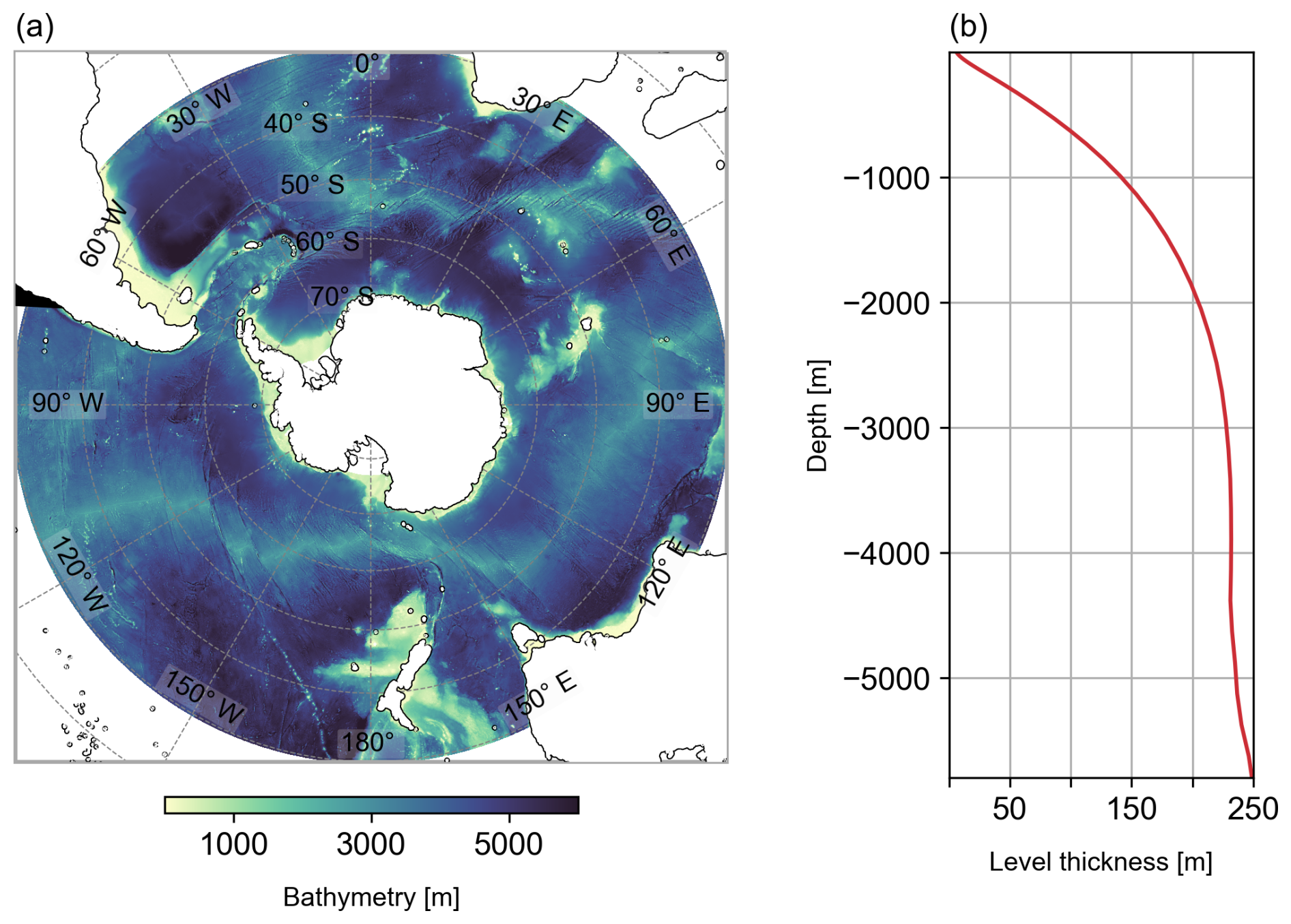
Figure 1 BIOPERIANT12 grid configuration (a) domain showing model bathymetry and (b) vertical grid cell thickness as a function of depth.

2.2 Initial conditions

To obtain a representative and stable surface ocean state, BIOPERIANT12 is initialised from rest, with temperature, salinity, and biogeochemical tracers derived from climatological data products. This model thus starts from a contemporary ocean state with large-scale climatological gradients and minimises spin-up. For the ocean, the initial temperature and salinity fields are taken from the World Ocean Atlas (WOA) Levitus January climatology (Locarnini et al., 2010). Sea ice is initialised using January ice climatology averaged over 1998–2007 from the ORCA12-MAL101 simulation, when sea ice extent is low. Thereafter, sea ice evolves freely under the dynamics of the LIM2 model, responding to the simulated thermodynamic and dynamic forcing.

Biogeochemical tracers are initialised from coarse-resolution observational climatologies which provide realistic large-scale distributions. Dissolved inorganic carbon (DIC), total alkalinity (TA) are obtained from the GLODAP annual mean climatology (Key et al., 2004); while nutrients including nitrate (NO₃), phosphate (PO₄), silicate (Si) and oxygen (O₂) are taken from the January monthly climatology of WOA09 (Garcia et al., 2013, 2010). Dissolved organic carbon and iron fields are inherited from the BIOPERIANT05-GAA95b simulation due to lack of climatological dataset and particularly the importance of iron to the region. BIOPERIANT05-GAA95b was initialised with the same biogeochemical tracers as above and with remaining tracers from global model initial conditions (ORCA2, NEMO Consortium, 2020). Its output provides an internally consistent distribution of the aforementioned fields for the SO and is thus also used for boundary conditions. The remaining tracers in PISCES are initialised with uniform values as per standard model defaults.

2.3 Boundary conditions

BIOPERIANT12 has one open lateral boundary to the north. Interannually varying boundary conditions for the dynamics were obtained from the global $\mathrm{1}/\mathrm{12}$° ORCA12-MAL101 simulation, using available 5 d averages for the period 1989–2009. While these physical boundary conditions are at a comparable resolution, suitable high-resolution biogeochemical boundary conditions were not available at the time of set-up. Therefore, biogeochemical fields were taken from the coarser $\mathrm{1}/\mathrm{2}$° BIOPERIANT05-GAA95b simulation. Rather than using the full interannual series, which in coarse-resolution models can result in biases in the seasonal and vertical structure of DIC, and hence in the simulated seasonal cycle of carbon (Mongwe et al., 2016), a climatological “normal year” boundary forcing was constructed. This consisted of 5 d averaged fields computed over the period 1995–2009.

At lateral solid boundaries, partial free-slip conditions are applied. Surface atmospheric forcing is provided by ERA-Interim reanalysis data (Dee et al., 2011), applied through the CORE bulk formulae. Wind stress components are prescribed at intervals of 3 h using the absolute wind formulation, which does not account for the surface ocean current effect on wind speed. Sea surface salinity is weakly restored to monthly Levitus climatology values. In addition, a restoring term is applied to Antarctic Bottom Water to counteract a known drift in ACC transport from deep water structure in the DRAKKAR models (Dufour et al., 2012).

2.4 Model evolution

The model is integrated over the 21 year period from 1989 to 2009, the same period for which the ORCA12 boundary conditions were available. A baroclinic time step of 360 s is used. During the first five years of integration (1989–1994), the surface ocean dynamics adjust to the imposed forcing and initial conditions, reaching a statistical equilibrium. Key indicators such as transport through the Drake Passage also stabilise during this period (Figs. S1 and S2 in the Supplement), and thus these years are designated as the spin-up phase. From 1995 onward, the simulation proceeds under quasi-equilibrated conditions, with 5 d averaged output saved for analysis. The final decade of the simulation (2000–2009) is used for evaluation.

While the focus of the configuration is on upper ocean processes, particularly in the top 1000 m, it is noted that a gradual drift in deep ocean temperature (below 400 m) becomes apparent from approximately 2002 onward (Fig. S1e–g). This drift does not affect the surface dynamics or the primary objectives of the study, but should be considered when using the model output for investigations involving deep ocean processes.

2.5 Model numerics

Advection of ocean tracers (temperature and salinity) is implemented with the TVD scheme, while passive biogeochemical tracers in PISCES tracers are advected using the MUSCL advection scheme. Lateral diffusion for both physical and biogeochemical tracers is applied via a Laplacian operator along isoneutral surfaces. Lateral advection of momentum uses a leapfrog scheme, and momentum diffusion implemented using a bilaplacian operator along geopotential surfaces.

Vertical mixing is represented using the turbulent kinetic energy (TKE) closure scheme. For background subgrid-scale mixing, vertical eddy viscosity and diffusivity coefficients are set, respectively, to 1.2 × 10⁻⁴ and 1.2 × 10⁻⁵ m² s⁻¹ from default configuration name lists, e.g. ORCA2 (NEMO Consortium, 2020). At the ocean floor, a diffusive bottom boundary layer scheme is employed along with an advective scheme to account for downslope transport in cases of dense water overlying lighter water masses (Gurvan et al., 2019). The bottom boundary is set with a nonlinear bottom friction formulation.

2.6 Computational requirements

Development of BIOPERIANT12 began following the deployment of the Lengau high-performance computing (HPC) cluster at the National Integrated Cyberinfrastructure System’s Centre for High Performance Computing (NICIS-CHPC) in late 2016. Lengau, a shared resource for the South African research community, comprises approximately 32 832 Intel Xeon CPU cores when fully operational. The final reference simulation presented in this study was completed in 2020. Due to constraints related to national electricity which reduced available compute capacity, system stability, and resource allocations, model runs required operational adjustments. To mitigate risks of unexpected interruptions and ensure continuity of simulations, restart files were written more frequently at the expense of increased storage usage.

After applying NEMO’s land elimination algorithm, which excluded 19 % of subdomains with no active ocean points, the simulation was run using 3240 CPUs. This configuration optimised the trade-off between model scalability and wall-clock time, while efficiently managing the regular output of ocean, ice, and biogeochemical fields at 5 d intervals, as well as the frequent writing of restart files.

3 Model evaluation

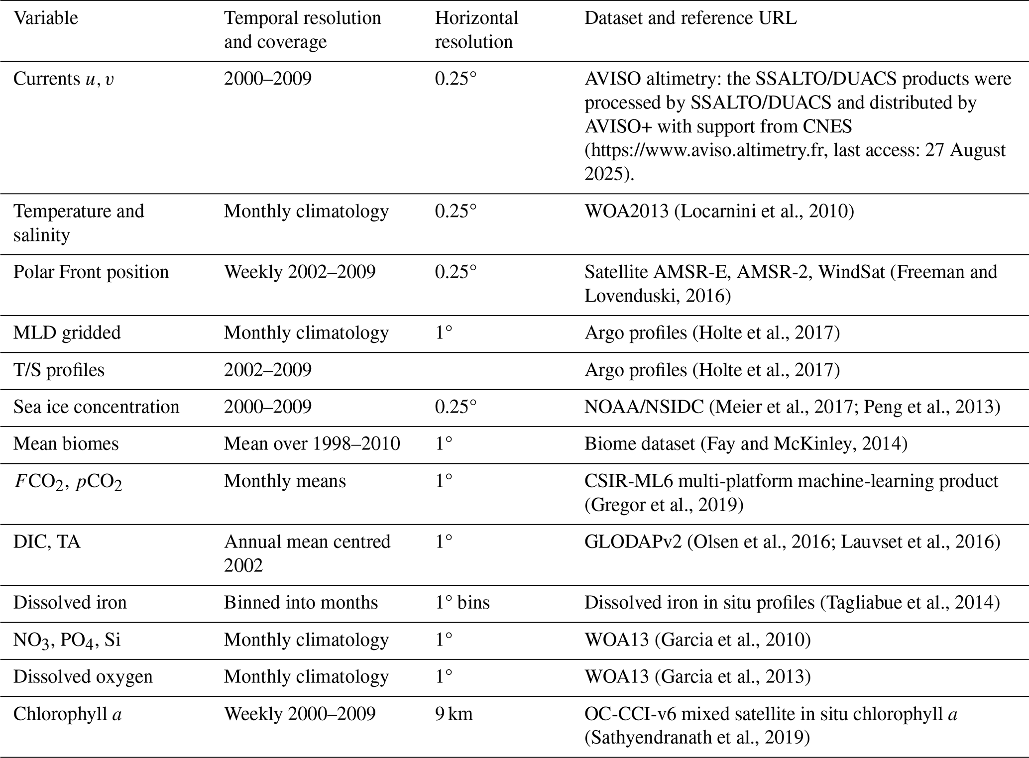
We evaluate the physical and biogeochemical fields of BIOPERIANT12 by comparing key upper-ocean metrics from the final 10 years of the experiment (2000–2009) against observational data (OBS), for which temporal and spatial coverage improves during the 2000s. Observational datasets are cited inline and listed in Table 1. Many of these datasets are low-resolution, gridded products, which are primarily applicable for evaluating the large-scale mean state.

(Locarnini et al., 2010)(Freeman and Lovenduski, 2016)(Holte et al., 2017)(Holte et al., 2017)(Meier et al., 2017; Peng et al., 2013)(Fay and McKinley, 2014)(Gregor et al., 2019)(Olsen et al., 2016; Lauvset et al., 2016)(Tagliabue et al., 2014)(Garcia et al., 2010)(Garcia et al., 2013)(Sathyendranath et al., 2019)

Table 1 Summary of observational datasets used for model evaluation.

As an initial comparison, we verify that the model reproduces the annual and seasonal mean states, followed by an assessment of the characteristics of temporal variability. In Sect. 3.1, we evaluate the model’s physical ocean and sea ice properties as indicators of model stability and general circulation, which in turn influence the BGC tracers. This evaluation is guided by the metrics proposed by Russell et al. (2018) for assessing the SO in coupled climate models and ESMs.

As a summary and precursor to further BGC evaluation, we present biome classifications and summarise model output in comparison to observations in Sect. 3.2. In Sect. 3.3, we focus on modelled carbon, while Sect. 3.4 provides further analysis of biogeochemical and biological properties.

3.1 Key physical ocean metrics in the Southern Ocean

3.1.1 Transport through Drake Passage

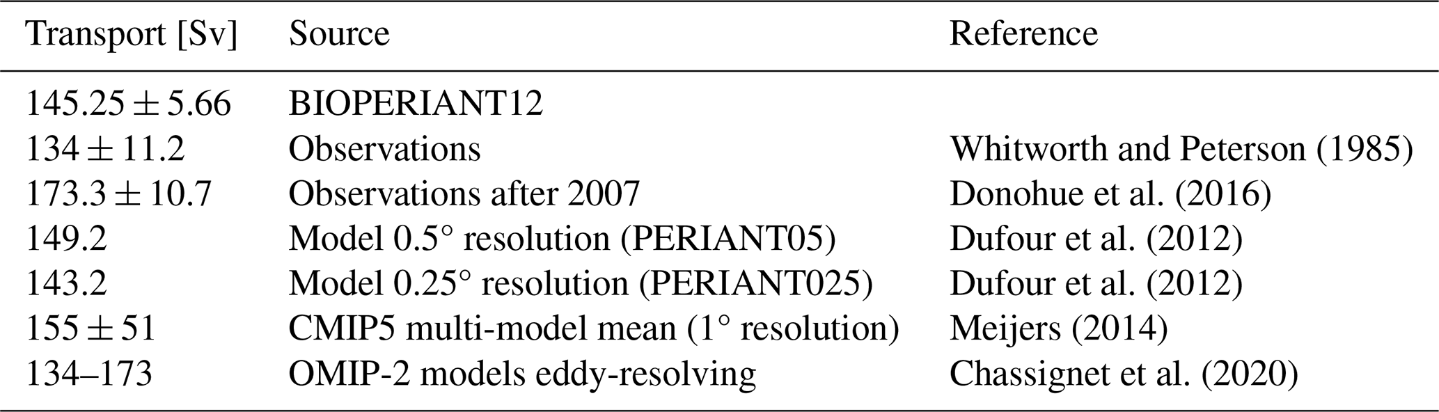
Transport of the ACC through the Drake Passage was calculated by integrating the model's zonal velocity from surface to bottom across 69° W. The time evolution of transport (Fig. S1b), shows that BIOPERIANT12 is stable after spin-up, with an annual mean transport through the Drake Passage from 2000–2009 at 145.25 ± 5.66 Sv. This value is comparable to observational estimates, as listed in Table 2, such as the widely accepted estimate of 134 ± 11.2 Sv by Whitworth and Peterson (1985). However, post-2007 estimates of transport are higher, such as 173.3 ± 10.7 Sv (Donohue et al., 2016) which is attributed to the increase in resolution in the observations. This higher value is used as the observational benchmark in model intercomparisons from CMIP3 to CMIP6 (Beadling et al., 2020). The mean transport of BIOPERIANT12 also compares well to its similar SO regional model predecessors, PERIANT05 and PERIANT025 (0.5 and 0.25° resolution, respectively), with respective mean transports of 149.2 and 143.2 Sv (Dufour et al., 2012). In addition, it aligns with estimates from global models such as the multi-model mean of 155 ± 51 Sv for CMIP5 models of mostly 1° resolution (Meijers, 2014) and the eddy-resolving Ocean Model Intercomparison Project phase 2 (OMIP-2) models which fall within the chosen observation range of 134–173 Sv (Chassignet et al., 2020).

Whitworth and Peterson (1985)Donohue et al. (2016)Dufour et al. (2012)Dufour et al. (2012)Meijers (2014)Chassignet et al. (2020)

Table 2 Drake Passage volume transport in BIOPERIANT12 compared with selected estimates from the literature.

3.1.2 Eddy kinetic energy (EKE)

The climatological annual mean surface EKE for 2000–2009 in BIOPERIANT12, compared to that derived from the AVISO $\mathrm{1}/\mathrm{4}$° gridded altimetry dataset, is shown in Fig. 2. The spatial distribution of EKE in the model is in general agreement with observations, capturing elevated EKE in regions associated with western boundary currents (WBC) and downstream of major topographic features. Zonally averaged EKE bands are comparable to SO models by Munday et al. (2021, Fig. 7a), although BIOPERIANT12 shows slightly higher EKE than their models, except for the WBC regions. For example, in the Agulhas Current region (Fig. S3), EKE is underestimated compared to observations, reflected as the lower zonal mean EKE between 36 and 43° S (Fig. 2a), possibly from missing dynamics around the Agulhas Retroflection region (15–45° E; Fig. S2b). Models at similar resolutions are able to represent the distribution patterns of EKE (e.g. ORCA12,  Rieck et al., 2015; Patara et al., 2016), although magnitudes may differ.

OMIP-2 ocean models (at ∼ $\mathrm{1}/\mathrm{10}$°) generally underestimate surface EKE, partially due to factors such as temporal averaging (Chassignet et al., 2020); regional effects: high EKE regions are eddy-rich but exhibit reduced spatial extent in OMIP-2 models compared to observations, while eddy-poor regions tend have greater coverage. In contrast, the regional model MOMSO (Dietze et al., 2020) overestimates EKE, which is attributed to the lower resolution of the observational dataset used for comparison. However, when the model’s spatial resolution was degraded to match that of the dataset, comparable magnitudes were obtained. Considering factors such as regional differences, the effect of winds (Patara et al., 2016), and the use of the absolute wind formula which neglects the effect of current-wind interactions which reduces eddy energy (Renault et al., 2016; Munday et al., 2021), BIOPERIANT12 provides a reasonable representation of mesoscale surface variability in the SO, supporting its use in exploring physical–biogeochemical interactions and addressing key BGC research questions.

3.1.3 Frontal structure

The SO fronts help describe the larger ACC structure, characterised by steep horizontal gradients and associated strong vertical motions, these fronts delineate regions with consistent water mass and nutrient properties, as well as regions of air–sea CO₂ in- and out-gassing, specifically CO₂ in-gassing north of the Polar Front (PF) and out-gassing between the PF and the marginal ice zone (Mongwe et al., 2018). Latitudinal shifts in the positions of these fronts can lead to local changes which affect heat and carbon fluxes and are thus used as a SO model evaluation metric by Russell et al. (2018).

The positions of the Subantarctic Front (SAF) and PF are chosen to represent the northern boundary and the central ACC, respectively. Following Russell et al. (2018), we apply a simplified subsurface temperature criterion, consistent with (Orsi et al., 1995), to identify these fronts: the SAF is defined by the 4 °C isotherm at 400 m and the PF by the 2 °C isotherm in the upper 200 m. This approach allows easy inter-model and model–observation comparisons.

In Fig. 3, we present the annual mean position and standard deviation of the SAF and PF in BIOPERIANT12 calculated from monthly means for the 2000–2009 period. These are compared to fronts derived from WOA13 monthly temperature climatology, the satellite-derived PF of Freeman and Lovenduski (2016), and the Orsi et al. (1995) dataset, as used by Russell et al. (2018). Overall, model fronts show spatial meridional variability consistent with the observation-derived fronts, but with a southward bias by up to 3° in latitude. This is accompanied by “pinching” of the fronts in regions of strong topographic influence, such as the Drake Passage, Campbell Plateau (170° E) and the Southwest (30° E) and Southeast (80° E) Indian Ridge, followed by diverging of the SAF and PF downstream.

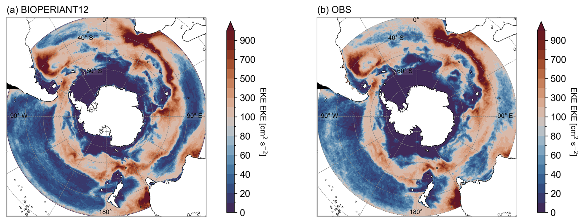
Figure 2 Annual mean surface EKE for the years 2000–2009 from (a) BIOPERIANT12 and (b) the AVISO $\mathrm{1}/\mathrm{4}$° dataset.

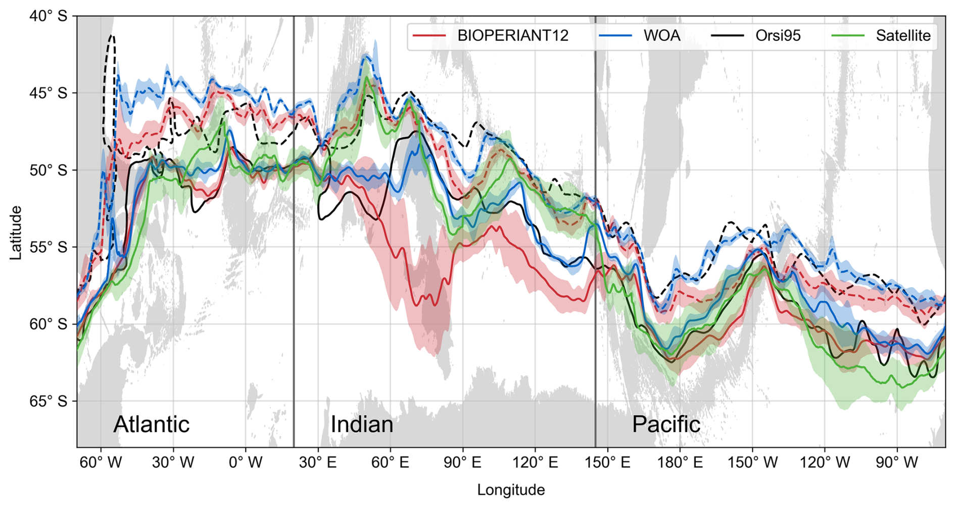
Figure 3 Annual mean latitudinal position of the Subantarctic Front (dashed line) and Polar Front (solid line) derived from temperature in BIOPERIANT12 (2000–2009), WOA13, the dataset of Orsi et al. (1995), and satellite SST Polar Front (2002–2009) from Freeman and Lovenduski (2016). Colour shaded regions are the standard deviation of the front using monthly mean temperatures. Grey-shaded regions show bathymetry shallower than 3000 m.

A notable discrepancy is observed in the modelled PF within the Indian Ocean sector, which may reflect the effects of temporal averaging or limited sampling of the observational datasets. At the Kerguelen Plateau (∼ 75° E), the PF follows either a northern or southern path but the temporal mean simulated PF is highly variable in latitude (standard deviation) aligning with the southern branch (Fig. S4). This contrasts with the observations that show the mean path favours the northern branch over the northern plateau (Dong et al., 2006; Wang et al., 2016). Similar to examples provided by Russell et al. (2018), the models evaluated (CMIP5 models at ∼ 100 km) do not completely or consistently capture similar patterns to the observations, reflecting model-specific biases as well as limitations of coarse resolution.

As shown in model EKE in Fig. 2, BIOPERIANT12 captures key aspects of SO mesoscale dynamics, including complex frontal behaviours such as branching, jet structures, and front–eddy interactions observed in satellite and in situ data (Freeman and Lovenduski, 2016; Chapman, 2017). Since frontal positions used a temperature-based criterion, they are sensitive to the representation of such mesoscale features. The high variability in frontal positioning driven by eddies in BIOPERIANT12 can lead to inconsistencies with observations, particularly in regions, such as the Kerguelen Plateau, where frontal locations are more strongly influenced by eddy activity than by the more stable meandering of coherent jets (Shao et al., 2015). Nonetheless, the model’s improved representation of mesoscale processes is expected to support more realistic exchange of water masses and biogeochemical properties (Rosso et al., 2020). While this complexity complicates direct model–observation comparison of frontal positions. The use of fronts remains valuable for delineating regions for analysis.

3.1.4 Mixed layer depth

To evaluate the MLD in BIOPERIANT12, we use in situ measurements given by the Argo floats database as our observational reference (Table 1). MLD for both the model and observations was calculated from temperature and salinity profiles following the de Boyer Montégut et al. (2004) density threshold of 0.03 kg m⁻³ relative to a reference depth of 10 m, a method that has been shown to be robust for SO profiles (Dong et al., 2008; Treguier et al., 2023). Although Argo float coverage has spatial and temporal gaps (Fig. S5), the temperature and salinity profiles collected by the floats provide direct measurements that capture real-world variability and mixing features, unlike reanalysis products which may introduce additional uncertainties due to model-dependent biases.

To ensure a consistent comparison, model MLDs were sampled according to the Argo observational coverage. Observed MLDs were binned onto a 1° × 1° regular grid and averaged into monthly intervals over the period 2001–2009. The same gridding and temporal averaging was applied to the model output, which was then subsampled to the same locations and months as Argo observations. The resulting seasonal–spatial patterns and amplitude in MLD are shown in Fig. 4.

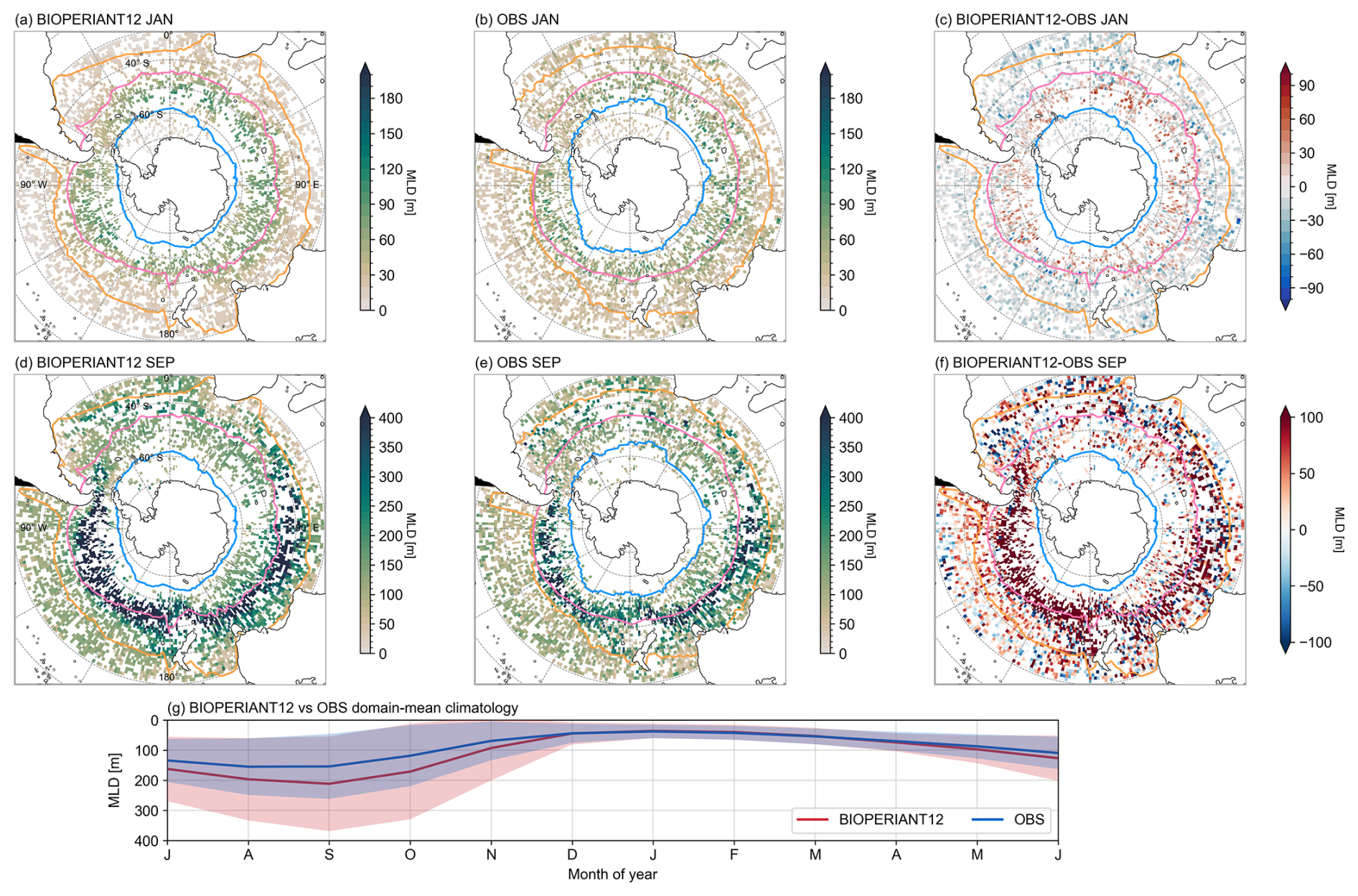
Figure 4 Seasonal comparisons of MLD from (a, d) BIOPERIANT12, averaged monthly and co-located to monthly averaged Argo MLDs on a 1°×1° regular grid, (b, e) Argo float observations, and (c, f) model–observation difference, for January and September climatologies, respectively. Maps are overlaid with the northern mean biome borders corresponding to model–data SO biomes. (g) Climatological seasonal cycle of monthly MLD, domain-averaged over the entire SO.

Overall, the spatial distribution of BIOPERIANT12 MLDs compares well with observations during both the minimum (January) and maximum (September) MLD months (Fig. 4a–b, d–e). However, in terms of magnitude, simulated summer MLDs within the ACC are too deep by ∼ 50 m, while MLDs north of the SAF are too shallow by a similar amount (Fig. 4c). In winter, BIOPERIANT12 generates deeper MLDs relative to observations, with a bias of ∼ 100 m in the Pacific sector of the SO (Fig. 4f). Despite this bias, the model correctly captures the pattern of deep winter mixed layers (> 400 m) in the Pacific and Indian sectors, indicating that it responds appropriately to atmospheric forcing and forms deep water masses in the expected regions.

The seasonal evolution of the MLD is a key diagnostic in the SO (Fig. 4g). The model reproduces the observed cycle of winter deepening and summer shoaling, with a Pearson correlation coefficient of R=0.97 for monthly climatologies. The shallow seasonal limit of simulated MLD aligns closely with observations during DJFM. However, the model departs from observed values around April, with standard deviations of the monthly mean MLDs showing the BIOPERIANT12 mixed layer extending over 100 m deeper than observations in September (MLD maximum). Treguier et al. (2023) showed that in OMIP models, even with horizontal resolutions ranging from 1° down to $\mathrm{1}/\mathrm{16}$°, MLD remains difficult to constrain, and higher resolution does not always result in improved representation of MLD in the SO. Nevertheless, despite its winter deep bias, the seasonal cycle and variability of BIOPERIANT12 MLD compares favourably with observations.

3.1.5 Ocean heat content (OHC) and temperature

Large-scale climatological temperature and 0–400 m OHC in BIOPERIANT12 compare well with observations in terms of spatial distribution (Fig. S6). A spatial map of model–observation differences reveals variability that appears linked to mesoscale activity (Fig. S7a–d), particularly given the coarser resolution of the WOA13 dataset ($\mathrm{1}/\mathrm{4}$°). In terms of magnitude, the model shows a higher domain mean 0–400 m OHC (∼ 13 × 10⁹ J m⁻², Fig. S7e) compared to observations, despite exhibiting a cool bias in sea surface temperature (SST) as shown in Fig. S7b, d, f. This discrepancy can be attributed to a warm bias in subsurface temperatures at 200 and 400 m (Fig. S7g). This result contrasts with the commonly observed warm SST bias in many SO models (Beadling et al., 2020).

Following initialisation with climatological fields and spin-up, upper ocean temperatures in the model (upper 200 m) exhibit no significant drift over the simulation period (Fig. S1c–d), even without the use of surface temperature restoring. Combined with the stable surface EKE discussed earlier, this suggests that surface ocean dynamics in BIOPERIANT12 remain stable throughout the analysis period. Given the consistency of model–observation biases, we do not attribute discrepancies in the physical or biogeochemical fields to spurious or transient model behaviour. Rather, remaining biases probably reflect systematic differences tied to consistent model behaviour or specific model design choices.

3.1.6 Sea ice

Sea ice plays a key role in setting the seasonal freshwater flux in the SO. Seasonal melting in the spring/summer and growth in autumn/winter strongly influence surface salinity and thereby affect both vertical and horizontal stratification dynamics (Giddy et al., 2021, 2023) as well as large-scale water mass transformation (Abernathey et al., 2016). For comparison with the model, observational mean monthly sea ice concentration data from the National Snow and Ice Data Center (NSIDC) for the period 2000–2009 were used (Table 1). Data show sea ice grows northward from the Antarctic continent during the winter months, reaching maximum extent in September and then melts, retreating southwards, towards the Antarctic continent reaching a minimum ice extent in February (Fig. 5).

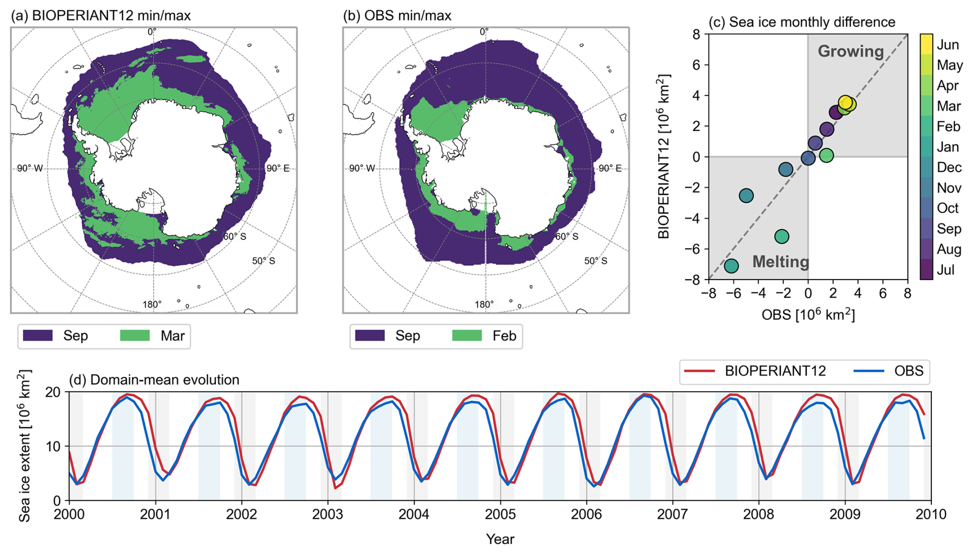
Figure 5 Climatological mean sea ice extent for the maximum (blue) and minimum (green) months for (a) BIOPERIANT12 and (b) NSIDC observations. (c) Climatological monthly mean sea ice extent difference indicating growth and melt for the BIOPERIANT12 simulation vs. NSIDC observations. (d) Time series of monthly mean sea ice extent from the BIOPERIANT12 model (red) and NSIDC observations (blue).

The spatial comparison of minimum/maximum sea ice extent (Fig. 5a, b) shows that the model reproduces the spatial pattern of winter maximum reasonably well but overestimates the total extent by approximately 1–2 million km², around 10 % of the observed winter maximum (Fig. 5c, d). Observations indicate a minimum in February, whereas the model shows similar minimum values spanning February and March. The timing of sea ice advance and retreat in BIOPERIANT12 suggests a realistic response to seasonal heat fluxes, with good agreement during winter maximum. However, the model does not melt enough ice in December (∼ 2 million km² compared to ∼ 5  million km² in observations) and compensates by continuing to melt through February (∼ 5 million km² in the model vs. ∼ 2 million km² in the observations), before both model and observations begin to show ice growth from March onwards (Figs. 5d, S8b).

Overall, BIOPERIANT12 captures a stable seasonal cycle in sea ice, with the largest interannual variability occurring during the summer months (Fig. S8b).

3.2 Biomes

3.2.1 Biome definition

To evaluate the biogeochemical and carbon fields, we apply the biome classification method of (Fay and McKinley, 2014), in preference to static geographic boundaries or physical definitions based on ocean dynamics (e.g. fronts). This approach combines large-scale physical and biogeochemical characteristics to delineate regions of biogeochemical similarity (biomes). Biomes are derived from climatological fields of SST, sea ice fraction, spring/summer chlorophyll a, and maximum MLD, using criteria defined in Fay and McKinley (2014, Table 1). SST and sea ice fraction criteria are used to distinguish between ice-covered, subpolar, and subtropical zones, while chlorophyll a and MLD criteria reflect environmental controls on biological production, such as vertical mixing, stratification, and seasonality (i.e. permanent vs. seasonal stratification).

Within the BIOPERIANT12 domain, the following biomes are identified (Fig. 6): in the SO, the ice biome (SO-ICE), the subpolar seasonally stratified biome (SO-SPSS), and the subtropical seasonally stratified biome (SO-STSS); further north, the subtropical permanently stratified biomes of the South Pacific (SP-STPS), South Atlantic (SA-STPS), and Indian Ocean (IND-STPS). A comparison between the BIOPERIANT12 biome distribution (Fig. 6a) and the observational product from Fay and McKinley (2014, Fig. 6b) shows that the model underrepresents the subtropical permanently stratified biomes (SP-STPS, SA-STPS, IND-STPS), resulting in approximately 60 % less area coverage than observed. Conversely, the SO-STSS and SO-SPSS biomes are slightly overestimated (Fig. 6c). As a result, only the SO biomes are used for subsequent aggregation and analysis. The observed differences may suggest some model–observation gaps (Figs. S9, S10) as well as the influence of mesoscale variability resolved by the model but absent from the coarser gridded datasets used to derive the observational biome product. This is discussed further in the Supplement.

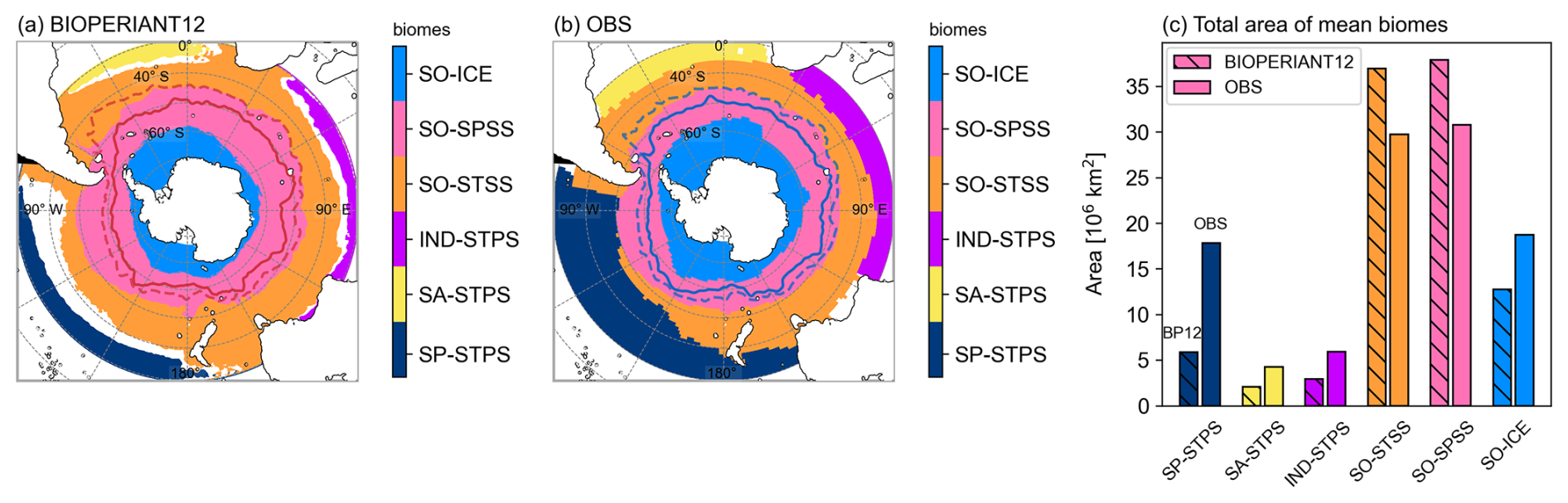
Figure 6 SO mean biome boundaries for (a) BIOPERIANT12 using the biome criteria definitions from Fay and McKinley (2014), (b) the observation-based mean biome dataset of Fay and McKinley (2014) south of 30° S (see the Supplement), and (c) total area per biome for BIOPERIANT12 (hatched bars, titled BP12) and for the dataset (plain bars, titled OBS). In the SO (below 30° S), six biomes are identified: SO-ICE, SO-SPSS, SO-STSS, IND-STPS, SA-STPS and SP-STPS. Annual mean frontal positions of SAF and PF are overlaid.

3.2.2 Biome characteristics

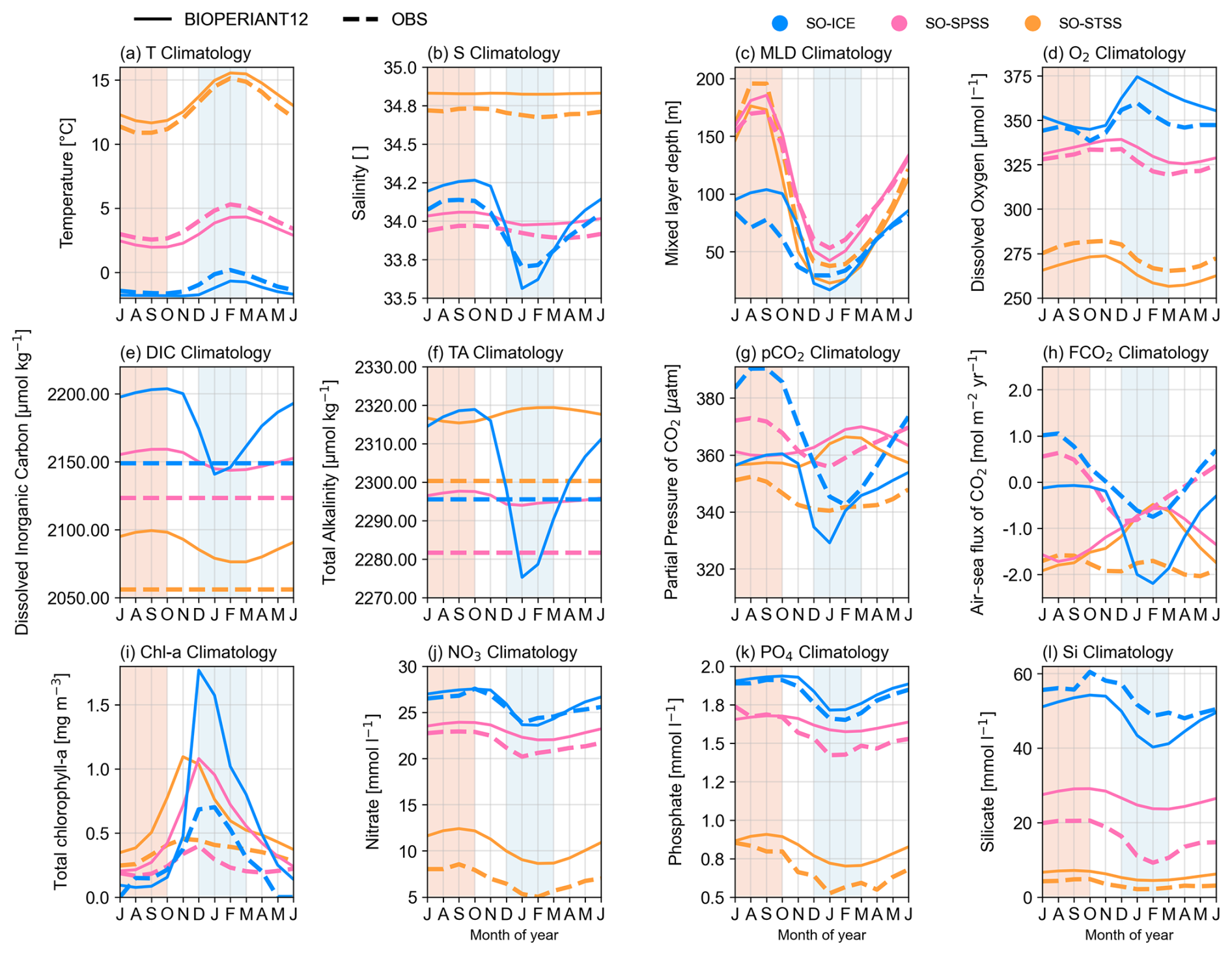
To characterise the seasonal cycle in the model, we present Fig. 7 the surface mean seasonal cycle of selected variables for each SO biome. To further contextualise the upper water column, vertical profiles per biome are shown in Fig. S11. In Table 3, we list the seasonal cycle at the surface using the mean and amplitude (difference between minimum and maximum), along with statistical metrics used to evaluate model–data agreement: the correlation coefficient (R), the ratio of standard deviations (RSD), the model reliability index (RI), and the seasonal cycle reproducibility (SCR). The same metrics are provided for 200 m depth in Table S1.

The correlation coefficient quantifies how well the timing and shape of the model seasonal cycle matches the observations. The RSD indicates how well the magnitude of seasonal variability in the model compares to that of the observations, with a value of 1.00 representing comparable variability between the two. The RI, or geometric root mean square error (Leggett and Williams, 1981; Doney et al., 2009), measures the normalised model–data bias for log-normal distributed variables, with a value of 1.00 indicating perfect agreement and 2.00 implying model error is comparable in magnitude to the data. SCR, defined by Thomalla et al. (2011), measures how well the climatological seasonal cycle captures the year-to-year evolution of a variable. It is calculated as the correlation between the full-resolution time series and its climatological seasonal cycle (see Fig. S12 for further explanation). SCR values above 0.85 indicate high seasonality, between 0.65–0.85 medium seasonality, and below 0.65 low seasonality. SCR was only calculated for observational datasets with adequate temporal resolution (i.e. higher than monthly).

Model–data differences can result from a combination of factors, including the characteristics and limitations of the observational datasets (Table 1), which often suffer from sparse sampling, low temporal and spatial resolution, and interpolation. Additional differences may arise from applying biome definitions to regions of high variability/EKE. Although EKE is not explicitly included in the biome classification, it has been shown to reduce partial pressure of carbon dioxide (pCO₂) biases and root mean square errors (Gregor et al., 2019). Further uncertainty is introduced through area-weighted domain averaging across large biomes. In contrast to regions dominated by intraseasonal variability, where observations are more difficult to constrain (Monteiro et al., 2015), the seasonal cycle metrics are expected to show stronger model data agreement in regions with seasonally driven dynamics (high SCR).

In general, the metrics (Table 3, Fig. 7) show the model's seasonal cycle agrees well with that the observed data, for example, the temperature seasonal cycle per biome is well represented. However, given that temperature is a criterion used in the biome definition, a reasonable agreement is expected. Therefore, we focus on the model–observation discrepancies, which highlight regions of interest. For the dynamics, there is a poor correlation of salinity in the SO-STSS region (R=0.62), which could be associated with the high mesoscale spatial and temporal variability in the model (low seasonality SCR =0.12). In the SO-ICE biome, high variability in salinity (RSD =1.55), MLD (RSD =1.56) as well as dissolved O₂ (RSD =1.66) to the significant influence of sea ice and freshwater dynamics in the model. This suggests that improvements or further investigation may be needed. For the BGC, poor model reliability for carbon, silicate, and chlorophyll, along with deviations in nutrient concentration, will be addressed in the proceeding sections.

Table 3 Seasonal cycle surface climatology per biome: BIOPERIANT12 (BP12) vs. observations (OBS). Area-weighted mean and amplitude (difference between maximum and minimum) are shown for each data source; SCR is the seasonal cycle reproducibility (correlation of the interannual varying time series with its climatological seasonal cycle) where temporal resolution allows; and for comparison correlation (correlation coefficient), RSD (ratio of BP12:OBS standard deviation), and Model Reliability Index (log-transform error) are included.

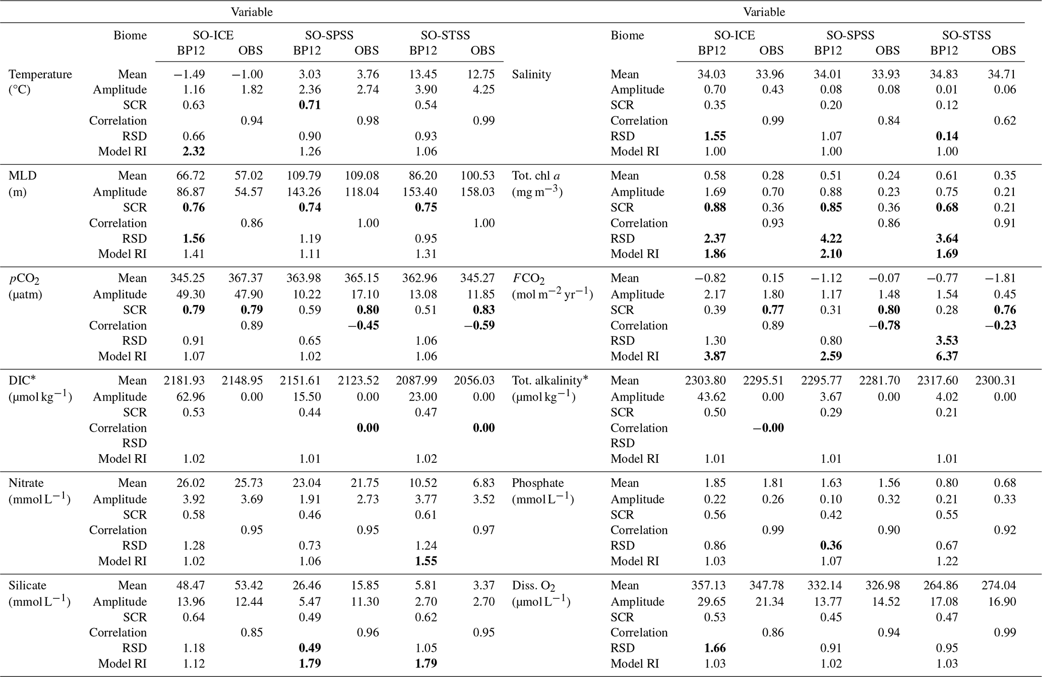
^* GLODAPv2 observations are an annual mean product.
RSD: SD of BP12 greater (less) than that of OBS by a factor of 1.5 (0.5). Correlation: BP12-OBS correlation coefficient less than 0.5.
SCR: BP12 greater than 0.65 (medium to high). Model RI: greater 1.5 (medium to high).

Figure 7 BIOPERIANT12 model (solid line) vs. observations (dashed line) surface seasonal cycle (2000–2009 climatology) spatially averaged per biome for selected variables. Biomes include SO-ICE (blue), SO-SPSS (pink) and SO-STSS (orange), corresponding to the map in Fig. 6.

3.3 Carbon

Recent studies have highlighted the importance of resolving intra-seasonal to seasonal variability for both anthropogenic and natural carbon fluxes in order to reduce uncertainties in mean annual fluxes and improve model projections (Monteiro et al., 2015; Mongwe et al., 2018; Nicholson et al., 2019; Djeutchouang et al., 2022,; Hauck et al., 2023; DeVries et al., 2023; Rustogi et al., 2023). We compare BIOPERIANT12 pCO₂ to the monthly observation-based product CSIR-ML6 (Table 1). CSIR-ML6 is a gridded 1° × 1° machine learning-based reconstruction of surface ocean pCO₂, derived from Surface Ocean CO₂ Atlas (SOCAT, Bakker et al., 2016) observations and satellite-based environmental predictors (Gregor et al., 2019).

Using SCR, as a metric of variability, a comparison between BIOPERIANT12 and CSIR-ML6 (Fig. 8) shows that model pCO₂ for the SO-STSS and SO-SPSS biomes is dominated by large regions of interseasonal variability (SCR = 0.59, 0.51, respectively), aligned with regions of high EKE (Fig. 2) which are not captured by the monthly CSIR-ML6 product (Fig. 8c). CSIR-ML6, instead, displays high seasonality in all three SO biomes with SCR values of 0.80, 0.80, 0.79 in the SO-STSS, SO-SPSS, and SO-ICE biomes, respectively (Table 3). These patterns are largely driven by seasonal surface fluxes and sea ice, although the monthly resolution of CSIR-ML6 may also contribute to the stronger seasonality.

This results in dissimilar pCO₂ seasonal cycles (Fig. 7g), as shown by weak correlations in the SO-STSS and SO-SPSS biomes (R= −0.59 and −0.45, respectively), in contrast to good model–data agreement in the SO-ICE biome. The SO-ICE biome is also strongly seasonally driven in the model (SCR = 0.79 for both model and data) and shows coherent model–data phasing (R=0.89), although the seasonal minima are offset by one month. Despite these differences, the small model–data bias in pCO₂ across all three biomes (RI between 1.02 and 1.07) and the broadly overlapping probability density functions (PDFs) for the SO domain mean pCO₂ (Fig. S13a) indicate some level of agreement in the mean state. These findings underscore the importance of mesoscale-resolving model resolution in the SO for capturing the variability of CO₂.

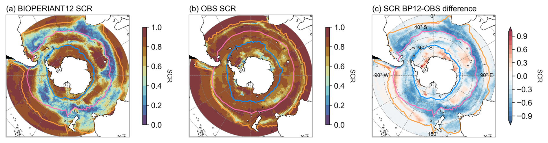
Figure 8 Seasonal cycle reproducibility of pCO₂ for (a) BIOPERIANT12, (b) CSIR-ML6 observation-based reconstruction, and (c) model–data difference. Maps are overlaid with the northern mean biome borders corresponding to model–data SO biomes.

The spatial distribution of pCO₂ shown in Fig. 9a–f illustrates the seasonal differences between the model and observations, with the model tending to overestimate pCO₂ in the SO-STSS and underestimate it in the SO-ICE biomes. Seasonal cycle phasing differences in the SO-SPSS and SO-STSS biomes are apparent in the interannual time series (Fig. 9i, k), where the model peaks in summer, in contrast to winter peaks in the data. The PDFs for pCO₂ (Fig.  9h, j, l) show generally broader distributions (i.e. higher standard deviation) in the model across all biomes, whereas the data exhibit clearer inter-biome distinctions, such as the narrower pCO₂ distribution in the SO-SPSS (Fig. 9j).

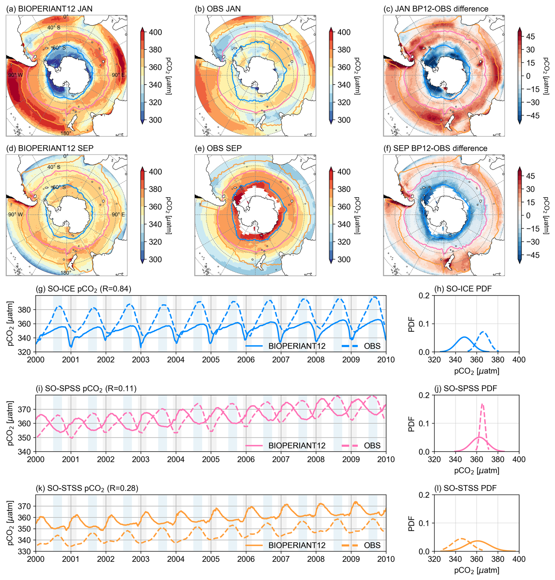
Figure 9 Seasonal comparison (January vs. September climatology) of pCO₂ for (a, d) BIOPERIANT12, (b, e) the CSIR-ML6 observation based dataset, and (c, f) the model–data difference. Maps are overlaid with the northern mean biome borders corresponding to model–data SO biomes. Evolution of area-weighted pCO₂ for model vs. data and corresponding PDF for (g, h) SO-ICE, (h, i) SO-SPSS, and (k, l) SO-STSS biomes.

The seasonal cycle differences of pCO₂ (and FCO₂) in the model SO-SPSS and SO-STSS biomes, relative to observations, may reflect the influence of different controlling mechanisms. In these biomes, the modelled pCO₂ seasonal maximum occurs in summer (JFM), in phase with the temperature maximum (Fig. 7a), but out of phase with the chlorophyll peak, which occurs approximately two months earlier (OND) (Figs. 7i, 13), and with the associated nutrient drawdown (NO₃ and Si; Fig. 7j, l). This suggests that in the SO-SPSS and SO-STSS biomes, the seasonal cycle of pCO₂ in the model is primarily driven by the thermal component (Mongwe et al., 2016). By contrast, the seasonal cycles of pCO₂ and FCO₂ in the SO-ICE biome show better phasing between model and data (Fig. 7g, h), and the seasonal cycles of temperature, chlorophyll, and nutrients are also more closely aligned (Fig. 7i–l). However, the amplitude of the seasonal chlorophyll maximum in the model is approximately double that of the observed estimate across all biomes. The climatology maps (Fig. 11) show that the model's overestimation aligns with regions of high chlorophyll in the data, which may lead to a larger contribution of biological components driving pCO₂, particularly in the SO-ICE biome.

It is important to note that observational products, particularly those based on underway pCO₂ observations used in reconstructions, carry significant seasonal biases due to sparse coverage during winter months (Djeutchouang et al., 2022). Consequently, the true magnitude and direction of the observed seasonal cycle of pCO₂ and FCO₂ in the SO remain uncertain (Gray et al., 2018; Landschützer et al., 2018; Gregor et al., 2019; Gruber et al., 2019; Bushinsky et al., 2019; Mackay and Watson, 2021). These seasonal sampling biases may also propagate into longer-term variability artefacts in the reconstructions (Hauck et al., 2023). The discrepancies between BIOPERIANT12 and the observational products, particularly in the SO-SPSS and SO-STSS biomes, may also reflect the model’s limited representation of key biological processes (discussed in the Supplement). We propose that a weaker seasonal vertical flux of DIC in the model, shown by a smoother upper-ocean DIC gradient compared to the dataset (Fig. S11), reduces the potential for DIC entrainment during periods of enhanced vertical mixing, thereby dampening the seasonal variability of DIC (Mongwe et al., 2016).

3.4 Biogeochemistry

3.4.1 Dissolved iron

Dissolved iron (dFe) limits phytoplankton growth across the surface of the SO, affecting the functioning of marine ecosystems and, consequently, the carbon cycle. It is therefore imperative that models accurately represent the spatial and seasonal distribution of dFe. In the SO, dFe is notoriously undersampled, it occurs at low (nanomolar, nM) concentrations, and its complex chemistry makes it difficult to observe. Here, we compare BIOPERIANT12 with a compilation of dFe observations collated by Tagliabue et al. (2012) over 2000–2009 (Fig. 10). BIOPERIANT12 captures the observed spatial distribution of upper ocean dFe concentrations, with elevated levels (>0.4 nM) near coastal boundaries, downstream and around sub-Antarctic islands (particularly evident around Kerguelen), and in the vicinity of the Agulhas Retroflection (Fig. 10a,c). In regions distant from land masses, simulated dFe concentrations are lower (<0.3 nM), seen in the observations (Fig. 10b). Overall, the simulated open ocean surface dFe range lies on the lower end of the observed spectrum; this is consistent with previous findings that PISCES tends to underestimate open ocean dFe in the SO. This is suggested to arise from the simplification of the biological processes in the model that affects iron cycling and supply (Aumont et al., 2015; Tagliabue et al., 2016; Nicholson et al., 2019).

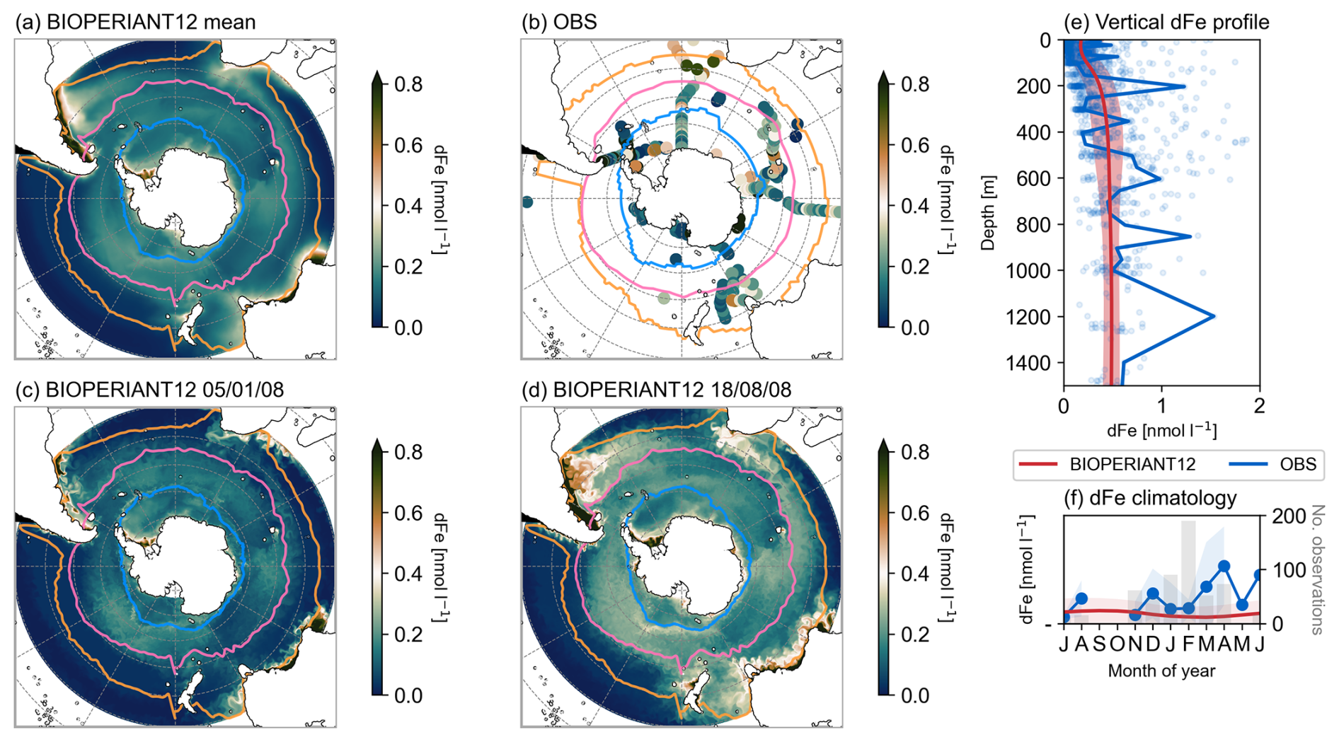
Figure 10 Surface (0–50 m) dissolved iron (dFe) concentration for (a) BIOPERIANT12 annual climatological mean (b) observations from 2000–2009 (Tagliabue et al., 2012). Seasonal snapshots of BIOPERIANT12 dFe for (c) summer (5 January 2008) and (d) winter (18 August 2008). (e) Climatological mean vertical distribution of dFe for BIOPERIANT12 (red line = mean; red shading = spatial standard deviation) and observations (blue). (f) Model vs. observation monthly climatology (lines) and standard deviation (shading); the number of observations per month is shown by grey bars.

The shape of the vertical dFe profile is important as it determines the amount of dFe that can be supplied to the surface ocean through processes such as deep winter convective mixing and mesoscale eddy activity (Tagliabue et al., 2014; Nicholson et al., 2019). BIOPERIANT12 reproduces the general features of the observed dFe profile (Fig. 10e), with low concentrations in the upper 0–100 m from biological consumption, and increasing concentrations with depth due to remineralisation of sinking organic material. Simulated dFe values compare reasonably well with observations in the upper 500 m, but tend to be lower at greater depths.

The scarcity of measurements during key seasonal transitions, particularly over winter (Fig. 10f), limits robust evaluation of the simulated seasonal surface dFe. Nevertheless, austral summer (DJF) is expected to exhibit low surface dFe due to biological consumption from spring to summer, while winter (JJA) is expected to show higher surface dFe as a result of vertical entrainment of subsurface iron during deep convective mixing (Tagliabue et al., 2012). These seasonal variations are captured by BIOPERIANT12 (Fig. 10f), as also shown in the summer and winter distribution snapshots in Fig. 10c and d, respectively.

3.4.2 Nutrients

Model RI values listed in Table 3 indicate that BIOPERIANT12 is able to reasonably reproduce the seasonal climatology of NO₃ and PO₄ with relatively comparable seasonal cycles (Fig. 7), particularly in the more southern biomes (e.g. RI values between 1.02 and 1.07 for both NO₃ and PO₄ in the SO-ICE and SO-SPSS biomes). However, simulated surface Si is less well represented (RI = 1.79 for both SO-SPSS and SO-STSS): in the SO-SPSS, the model mean Si concentration (26.46 mmol L⁻¹) is substantially higher than observed (15.85 mmol L⁻¹), with a reduced seasonal amplitude (5.47 vs. 11.3 mmol L⁻¹) and only half the variability (model RSD = 0.49). These discrepancies may stem from uncertainties in the silica dissolution process and its formulation in the model Aumont et al. (2015), which may, in turn, affect the simulated diatom distribution.

While model PO₄ exhibits reasonable mean values, its variability is also underestimated, at only 36 % of that observed. It is important to note that much of the observational dataset is biased towards the productive season (austral summer) in the SO, which may result in lower observed surface nutrient values (Figs. 7, S16).

At 200 m depth, however, RI values for all three nutrients indicate good model–data agreement (ranging between 1.00 and 1.30; Table S1, Fig. S17). Nutrient concentrations at this depth are stable in the model, with standard deviations smaller than those from the observational climatology (Fig. S11). Over the model simulation period (Figs. S16 and S17), there is a slight declining trend in nutrient concentrations, particularly noticeable in the SO-SPSS both at the surface and at 200 m, which should be taken into consideration in process studies.

3.4.3 Surface chlorophyll

To evaluate the model's representation of biological variability, we compare surface chlorophyll concentrations from BIOPERIANT12 with the OC-CCI v6 satellite-derived dataset (Table 1) gridded at a comparable resolution of 9 km and aggregated weekly to match the model output. BIOPERIANT12 broadly captures the spatial patterns of surface chlorophyll concentrations (Fig. 11). For example, the model captures enhanced chlorophyll levels near continental margins and in frontal regions such as the Subantarctic Zone (SAZ; not shown), while lower chlorophyll concentrations are simulated in more oligotrophic regions such as the South Pacific sector of the SO. However, there are notable differences in the summer pattern (Fig. 11a–c), such as the overestimation of the spatial extent of elevated chlorophyll concentrations associated with shallow topography. While the overestimation of chlorophyll occurs regardless of spatial aggregation, the inclusion of these elevated regions within biome definitions contributes to the overestimation of biome-mean values and results in variability more than twice that observed (RSD >2.00 in Table 3).

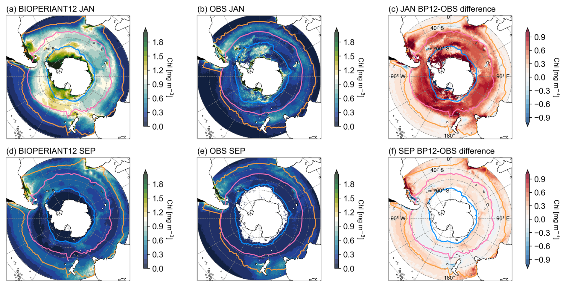
Figure 11 Climatological total chlorophyll concentrations for January and September for (a, b) BIOPERIANT12 and (d, e) the OC-CCI observation-based product. SCR of surface chlorophyll for (c) BIOPERIANT12 and (f) observations. Model vs. observation seasonal cycle of surface chlorophyll for (g) SO-ICE, (h) SO-SPSS, and (i) SO-STSS biomes.

SCR (Fig. 12) suggests the overestimation of model chlorophyll arises from the temporal variability: the response of model chlorophyll is strongly seasonal, whereas satellite indicates strong intra-seasonal variability. Nevertheless, BIOPERIANT12 shows good agreement with OC-CCIv6 in terms of the climatological seasonal cycle (Fig. 7i), with correlations greater than 0.86 in all SO biomes, and the timing of peak chlorophyll with bloom maxima generally occurring in December (Fig. 13) with timing differences within 14 d. A biome-mean comparison (Figs. 13, S18) further shows that bloom initiation and termination, defined using the biomass threshold method of 5 % (Ryan-Keogh et al., 2023), are reproduced with varying degrees of success. In the SO-STSS biome, both the model and observations show bloom onset in August and decline in May. For the SO-SPSS biome, both datasets agree on a September onset, the model sustains the bloom approximately 93 d longer than observed, extending into June (vs. March in data). In the SO-ICE biome, while model–data agree on termination in May, the model bloom initiates 3 months after observations (October vs. August).

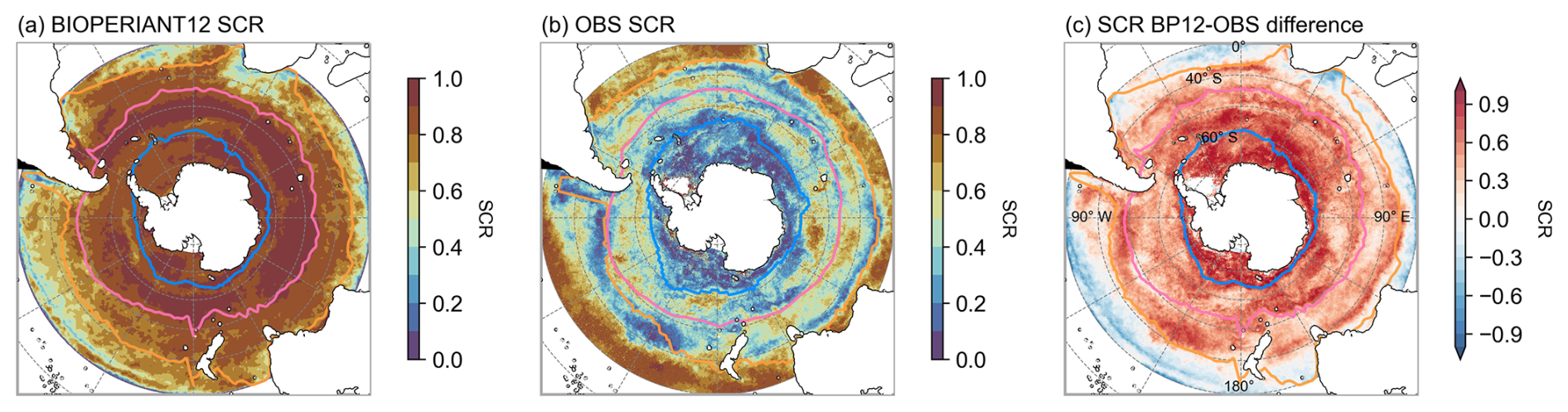
Figure 12 Seasonal cycle reproducibility (SCR) of surface chlorophyll concentration for (a) BIOPERIANT12, (b) the OC-CCIv6 observation-based product, and (c) model–observation SCR bias.

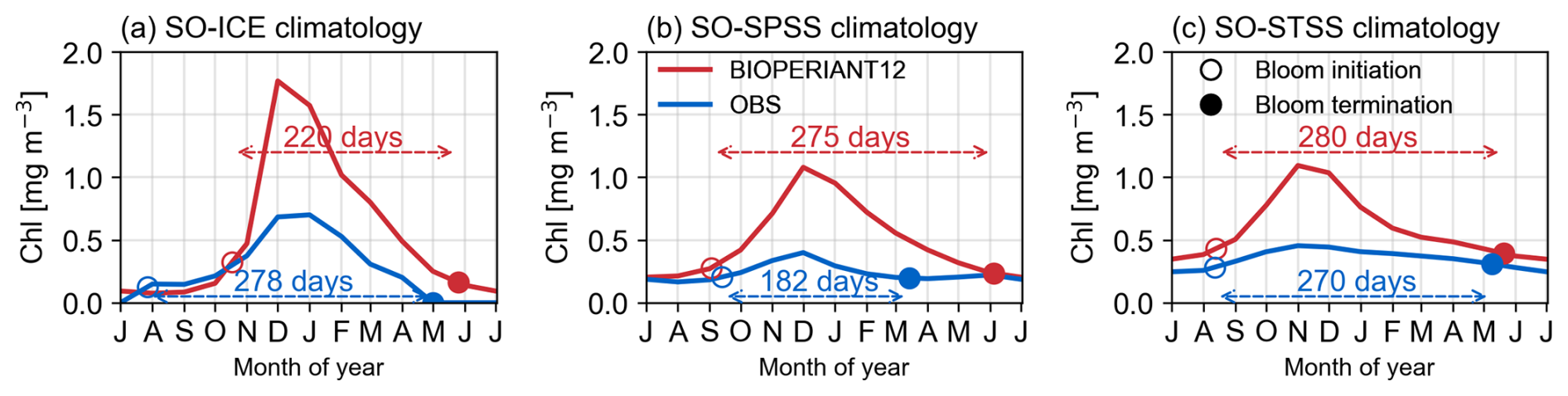
Figure 13 Climatological bloom characteristics from BIOPERIANT12 and the OC-CCI observation-based product overlaid on the seasonal cycle of surface chlorophyll for (a) SO-ICE, (b) SO-SPSS, and (c) SO-STSS biomes.

These results demonstrate that while BIOPERIANT12 captures key spatial and seasonal features of chlorophyll in the SO, it probably underrepresents the higher-frequency biological variability evident in observations; even at mesoscale-resolving resolution. Underlying ocean dynamics that could be further improved in BIOPERIANT12 include the representation of shelf-slope dynamics and mixing processes. For instance, enhanced vertical mixing may prolong bloom duration, as seen in the SO-SPSS biome, where the modelled bloom persists nearly three months beyond satellite-based estimates. Additionally, the biogeochemical processes that drive productivity and blooms in the SO such as nutrient limitation (especially iron), fixed phytoplankton stoichiometry, and prescribed chlorophyll-to-carbon ratios, also require further refinement. The overestimation of chlorophyll magnitude and mismatches in bloom timing suggest that processes governing phytoplankton bloom dynamics, particularly those modulated by mesoscale physical variability, warrant further investigation.

However, chlorophyll model vs. satellite data comparisons are inherently challenging, with both sources subject to internal biases and uncertainties. Limitations in satellite observations arise from the satellite itself, such as solar zenith angle, cloud cover, and sea ice contamination, particularly at high latitudes; as well as from environmental complexities of the SO such as the presence of subsurface chlorophyll maxima and algorithms not well suited to these conditions (Clow et al., 2024; Aumont et al., 2015).

4 Conclusions

The complex dynamics of the SO have been the focus of extensive research, particularly due to their role in the climate system and carbon cycle. While model intercomparisons help expose the strengths and weaknesses of ESMs, individual models remain intricate systems defined by numerous interacting assumptions, making the isolation of specific biases challenging. In contrast, BIOPERIANT12 offers a relatively simpler, high-resolution coupled ocean–ice–BGC configuration with a stable and realistic mean state as shown by the evaluation of the physical ocean metrics. Thus, providing a useful reference framework for process studies, bias diagnostics, and future model experimentation.

Despite its mesoscale-resolving resolution, BIOPERIANT12 still shows notable limitations in simulating key biogeochemical processes in the SO. In particular, the model overestimates chlorophyll concentrations and exhibits variability more than twice that of satellite-based observations across all SO biomes. The timing and duration of phytoplankton blooms also differ from observations, with blooms sometimes initiating too late or persisting beyond observed termination, as in the SO-SPSS biome. These discrepancies highlight the importance of mesoscale processes and their interactions with BGC, such as shelf-slope dynamics, vertical mixing, and nutrient limitation, especially of iron. While some regional biases remain, there are systematic biases attributable to the model formulation and not the configuration design, such as the commonly used fixed chlorophyll-to-carbon ratios and phytoplankton stoichiometry which may limit the model to fully capture the dynamical nature of SO productivity. These issues are common to many biogeochemical models and point to structural limitations beyond just this configuration.

While this model description paper focuses on introducing the BIOPERIANT12 platform and evaluating its large-scale physical and biogeochemical patterns, the use of low-resolution gridded observational datasets inherently limits the depth to which model–data mismatches can be interpreted (Djeutchouang et al., 2022). In high-resolution configurations such as BIOPERIANT12, discrepancies with observations often reveal limitations, not only in the model formulation but also in the observing systems themselves. BIOPERIANT12 offers an opportunity to diagnose and potentially reduce structural biases; however, doing so requires an equally robust understanding of observational uncertainty.

For physical processes, this has been discussed in the context of the development and constraining of ocean circulation models by Fox-Kemper et al. (2019). In the context of BGC, particularly for surface carbon fluxes, understanding the drivers of primary production and bloom dynamics is critical (Thomalla et al., 2023). Although satellite products have the necessary spatio-temporal coverage to inform these processes, there are limitations as addressed by Clow et al. (2024). For surface ocean pCO₂, the biases and sampling limitations are discussed by Djeutchouang et al. (2022), highlighting the challenges of sparse coverage.

These findings underscore the need to refine both the physical and biogeochemical components of models to better represent sub-seasonal variability and the complex drivers of productivity in the SO. With this goal in mind, BIOPERIANT12 provides a coherent, high-resolution, three-dimensional dataset that is well-suited for understanding upper-ocean physical-biogeochemical processes and interactions on daily to interannual time scales. It has already proven useful for investigate SO sampling biases through observing system simulation experiments (e.g. in air–sea CO₂ flux estimates, Djeutchouang et al., 2022), and to understand the role and contributions of mesoscale features in shaping carbon and heat distributions (Smith et al., 2023). While the computational demands of this configuration constrain long-duration sensitivity studies, the insights gained from model–observation mismatches point to specific regions and processes where improvements are needed, and where newer model versions and higher-resolution datasets can help advance our understanding.