GEOCLIM7, an Earth system model for multi-million-year evolution of the geochemical cycles and climate

The numerical model GEOCLIM, a coupled Earth system model for the long-term biogeochemical cycle and climate, has been revised. This new version (v 7.0) allows a flexible discretization of the oceanic module for any paleogeographic configuration, coupling to any general circulation model (GCM), and the determination of all boundary conditions from the GCM coupled to GEOCLIM, notably the oceanic water exchanges and the routing of land-to-ocean fluxes. These improvements make GEOCLIM7 a unique, powerful tool, devised as an extension of GCMs, to investigate the Earth system evolution at timescales (several million years) and with processes that could not be simulated otherwise. We present a complete description of the model, whose current state gathers features that have been developed and published in several articles since its creation and some that are original contributions of this article, like the seafloor sediment routing scheme and the inclusion of orbital parameters. We also present a detailed description of the method to generate the boundary conditions of GEOCLIM, which is the main innovation of the present study. In a second step, we discuss the results of an experiment where GEOCLIM7 is applied to the Turonian paleogeography, with 10 Myr orbital cycle forcings. This experiment focuses on the effects of orbital parameters on oceanic O₂ concentration, particularly in the proto-Atlantic and Arctic oceans, where the experiment revealed the largest O₂ variations.

1 Introduction

The evolution of climate during Earth's history is closely associated with atmospheric CO₂, arguably the most important greenhouse gas, at least in the Phanerozoic eon. At this timescale (several million years), variations of atmospheric pCO₂ are controlled by the geological carbon cycle, characterized by the exchanges between the solid Earth and superficial reservoirs (atmosphere, ocean, and biosphere). Furthermore, the carbon cycle is interlinked with other global biogeochemical cycles – oxygen, for instance – all of them interacting with climate. A first challenge for understanding the past variations of pCO₂ and climate is the multiplicity of cycles with different residence times (∼10 kyr to ∼10 Myr) and feedbacks between them, also operating with different timescales. A single process can thus affect several geochemical cycles and have different impacts at different timescales (e.g., Maffre et al., 2021). Deciphering the processes and feedbacks to explain past variations of climate was the motivation for the development of early geological carbon cycle models, the most iconic being GEOCARB (Berner, 1991, 1994; Berner and Kothavala, 2001); more recently developed ones include GEOCARBSULF (Berner, 2006) and COPSE (Lenton et al., 2018). These models, though highly efficient for the targeted timescale, face another challenge in the understanding of climate evolution, which is the spatial scales relevant for the processes. Carbon and other elemental fluxes can be significantly affected by relatively small areas, such as restricted oceanic basins or narrow mountain ranges. Yet, pCO₂ is ontologically a global variable, and its evolution can only be understood with a global-scale modeling approach. The spatial discretization of the whole Earth to simulate geochemical cycles is typically done by Earth system models (ESMs), such as PISCES (Aumont et al., 2015), or Earth system models of intermediate complexity (EMICs), such as CLIMBER-X or iLOVECLIM. These models often focus on oceanic biogeochemistry and explicitly calculate climate dynamics. Indeed, a third challenge is to accurately quantify the feedbacks between the climate and geochemical cycles, which is especially critical for CO₂ (Walker et al., 1981; Berner and Caldeira, 1997). Those feedbacks also need to be investigated with a relatively high spatial resolution because of the high geographic heterogeneity of climate fields (e.g., temperature, precipitation, oceanic upwelling, and deepwater formation). Nondimensional box models – such as COPSE and GEOCARBSULF – use parameterizations of those feedbacks between mean climate and global fluxes. Such parameterizations are often based on modern observations, or some specific climate simulations, and may not hold for radically different paleogeography and geodynamics settings. On the other hand, ESMs and EMICs are limited to a few 10 to 100 kyr long simulations because of their computational cost and because of implicit assumptions that become inconsistent at longer timescale: closed ocean–atmosphere system (e.g., no imbalances allowed between external sources and sinks), fixed concentration of slowly varying species (e.g., atmospheric oxygen, oceanic sulfate), or restoring conditions imposed to keep fixed the global content of nutrients (Aumont et al., 2015).

A notable technical gap exists between long-term low-resolution box models and short-term high-resolution Earth system models. In the last two decades, several models have been developed to fill that gap: cGENIE (Ridgwell et al., 2007; Colbourn et al., 2013; Van De Velde et al., 2021; Adloff et al., 2021), LOSCAR (Zeebe, 2012), CANOPS (Ozaki et al., 2011, 2022; Ozaki and Tajika, 2013), SCION (Mills et al., 2021), and CH2O-CHOO-TRAIN (Kukla et al., 2023). Each of them addresses the mentioned challenges in a specific way to benefit of or at the expense of the oceanic resolution, the continental resolution, the computation of climatic feedbacks, and the possibility for long time integration. In this contribution, we present the model GEOCLIM, which is also meant as a “bridge” between GEOCARB-style models and ESMs and addresses the resulting technical challenges in a unique way through coupling with a high-resolution climate model – or general circulation model (GCM). GEOCLIM thus combines the benefits of an intermediate oceanic resolution (similar to LOSCAR or CANOPS), a continental resolution similar to a GCM, the physically based computation of climate dynamics and climatic feedbacks, and a calculation performance of 0.2 to 6 million simulated years (depending on the configuration) per hour of computation on a standard laptop or a single CPU.

The initial motivation for building GEOCLIM was to move to a much more physically based calculation of the continental runoff (defined here as the difference between the rainfall and the evapotranspiration). Firstly, many processes depend on runoff (e.g., erosion, weathering), but also some of these dependencies are nonlinear, calling for a geographical distribution of the calculation of runoff. The first version of GEOCLIM was built by combining the geochemical cycle module COMBINE (Goddéris and Joachimski, 2004) with a 1D energy balance mode (EBM), allowing the calculation as a function of the latitude. Nevertheless, EBMs do not include a process-based description of the water cycle. Later versions of GEOCLIM therefore coupled COMBINE to the EMIC CLIMBER-2 (Donnadieu et al., 2004) and then to the 3D GCM FOAM (Donnadieu et al., 2006). Since 2006, the successive versions of GEOCLIM have all included a coupling with a GCM. The drawback of including the physics of climate is that it is not possible to achieve a direct coupling between the GCM and the geochemical module. Hence, GCM simulations must be conducted prior to running GEOCLIM, and the actual climate fields used by the geochemical code are recomputed from the GCM outputs by (multi)linear interpolation.

The revised version of GEOCLIM we present in this contribution is the seventh (GEOCLIM7). Taking advantage of the extensive development of paleoclimate modeling in recent years, the architecture of GEOCLIM was redesigned to be used as an extension of a GCM, aiming to investigate the interactions between climate dynamics and geochemical cycles. With this new version of GEOCLIM, any GCM can be (indirectly) coupled to GEOCLIM. Boundary conditions such as paleogeography, topography, river routing, and bathymetry are, as far as possible, determined by the GCM simulations whose climatic fields (land temperature and runoff, oceanic temperature, and circulation) are used to force GEOCLIM. The choice of the oceanic discretization of GEOCLIM – which is essentially an upscaling of the GCM grid – has been made flexible in GEOCLIM7, so it could be modified to account for peculiarities of the studied time period and inspired directly by the GCM results (e.g., where does deepwater formation take place, and which oceanic basins are isolated from others?). This connection to a GCM offers the advantage of getting processes such as exchange water fluxes between oceanic boxes, distribution of continental erosion rates, and oceanic sedimentation rates based on a mechanistic computation and internally consistent within our modeling framework.

The version of GEOCLIM we present here is the result of successive developments partially described in multiple publications (Goddéris and Joachimski, 2004; Donnadieu et al., 2006; Arndt et al., 2011; Maffre et al., 2021). A centralized description of the model is essential to avoid information being scattered across multiple contributions, each with its own particularities. Moreover, we have invested significant effort in enhancing the influence of ocean dynamics in GEOCLIM. Previous EMIC and Earth system model simulations (e.g., ESM) have demonstrated that the central Atlantic basin was a preferential location for anoxia during the Cretaceous, not only due to its restricted nature but also because it was the terminus of thermohaline circulation. One of our objectives was to find out how to represent the Cretaceous ocean in a still simplified box model to get such gradients in the oxygenation between the Pacific and the central Atlantic. Another motivating factor for our new development was the findings of Sarr et al. (2022) regarding the potential impact of orbital oscillations on the degree of anoxia in the central Atlantic during the Cretaceous. Our objectives are then twofold: (1) to represent a 3D oceanic field within a simplified multi-box model and (2) to incorporate periodic changes due to orbital oscillations, with the ultimate goal of providing the community with a hybrid Earth model capable of simulating the impact of anoxic events and their internal variability at the orbital scale.

This article is then organized into three parts that are rather complementary. Section 2 gives the complete model description, with a brief overview (Sect. 2.1), followed by the descriptions of the oceanic geochemistry (Sect. 2.2), early diagenesis (Sect. 2.3), and continental modules (Sect. 2.4), as well as the coupling between them (Sect. 2.5). For each of these subsections, we highlight what changes have been made, as the case may be, and provide reference for the last published version of the code. Section 3 concerns the generation of GEOCLIM's boundary conditions from GCM simulations, which is the major novelty of this contribution. Continental boundary conditions are discussed in Sect. 3.1, oceanic ones in Sect. 3.2, land-to-ocean routing in Sect. 3.3, and other boundary conditions in Sect. 3.4. Finally, Sect. 3.5 details the current model calibration. The third part of the article (Sect. 4) presents the results of a numerical experiment with GEOCLIM7 to study the impact of orbital cycles on geochemical cycles around the Cenomanian–Turonian boundary, with a focus on ocean oxygenation. For this specific study, GEOCLIM was coupled to the GCM IPSL-CM5A2 (Sepulchre et al., 2020), which is the standard version of the IPSL climate model used for deep-time (up to 100 Ma) paleoclimate studies. This study illustrates how GEOCLIM7 can supplement studies conducted with a GCM and an ESM and shed light on new processes.

2 Model description

2.1 Overview

The GEOCLIM model is designed for multi-million-year transient simulations. It couples different modules together:

• a 3D climate model which generates runoff and temperature fields over the continents and, when needed, the oceanic temperature and circulation.
  

• a box model describing the main oceanic biogeochemical cycles and the atmosphere for some of the cycles (carbon and oxygen).

• a simplified model describing the early diagenesis reactions inside the oceanic sediments.

• a model describing the physical erosion and chemical weathering reactions over the continents.

The last three modules have been developed by the authors and are extensively described in the following sections (2.2, 2.3, and 2.4, respectively).

2.2 Oceanic module

The GEOCLIM oceanic module is a box model which simulates the time evolution of the carbon (including the ¹³C isotopic signature), alkalinity, calcium, oxygen, phosphorus, and strontium (including the ${}^{\mathrm{87}}\mathrm{Sr}{/}^{\mathrm{86}}\mathrm{Sr}$) cycles. This model is a box model which captures the horizontal and vertical structure of the global ocean. Each box is assumed to be a well-mixed oceanic unit (for instance, the deep polar north oceanic reservoir). One box represents the atmosphere. The values of all the parameters of the oceanic module of GEOCLIM can be found in Tables 1 (for main variables) and 2 (for tracers). Appendix A describes additional empirical relationships regarding the fundamental chemical constant (e.g., acidity and solubility constants), including their dependence on temperature, pressure, and salinity. The oceanic module does not calculate the physical mixing of the ocean, which is prescribed (but can be changed over the course of a run). Also, the GEOCLIM model does not calculate the salinity over the course of a run. Salinity is prescribed for each oceanic basin. It can be changed arbitrarily during a simulation.

Table 1 Oceanic module parameters for main variables. The six chemical constants $K_{\text{sp}}^{\mathrm{o}}$, ${\mathit{\beta }}_{{\mathrm{O}}_{\mathrm{2}}}$, ${\mathit{\beta }}_{{\mathrm{CO}}_{\mathrm{2}}}$, K_c1, K_c2, and K_b are not actual parameters since they depend on temperature, salinity, and pressure. Their computation is described in Appendix A.

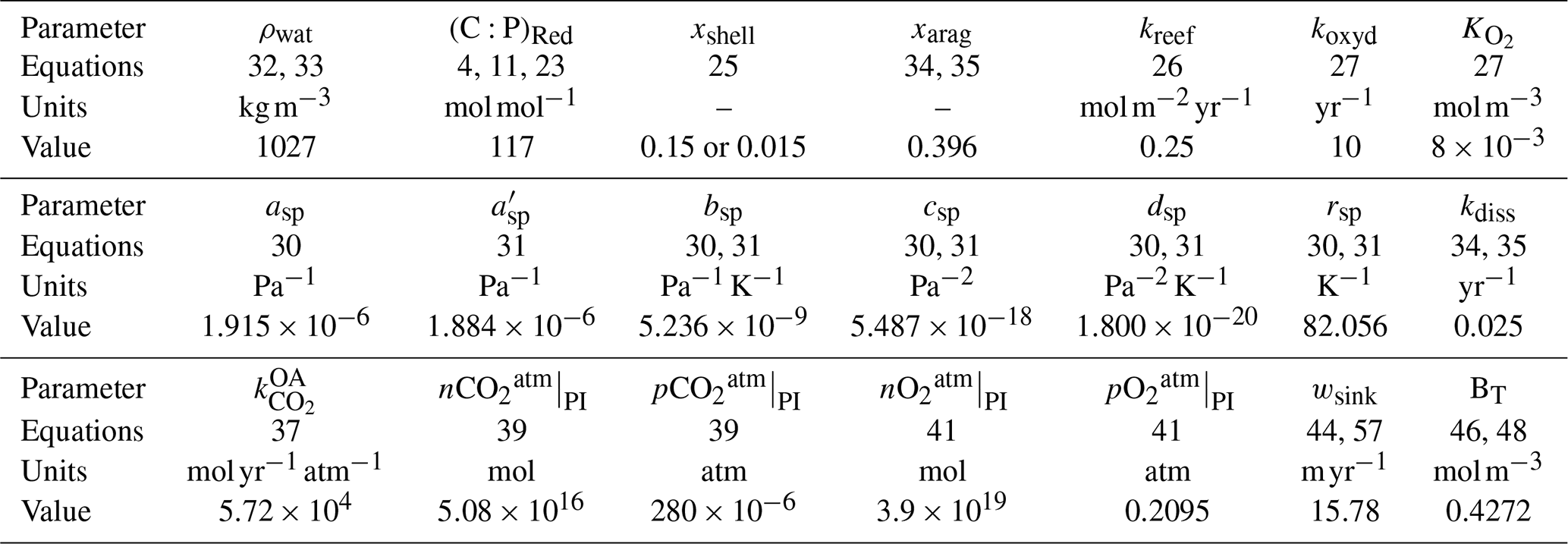
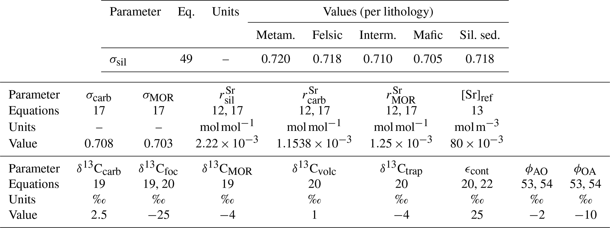
Table 2 Oceanic module parameters for tracers and isotopic variables. The two isotopic equilibrium fractionation parameters ϵ_D1 and ϵ_D2 are not, strictly speaking, parameters since they depend on temperature. Their computation is described in Appendix A.

2.2.1 Definition of GEOCLIM ocean–atmosphere boxes

By default, GEOCLIM discretizes the ocean–atmosphere in 10 boxes in the following order:

1. Northern high latitudes (latitude >60° N) surface (depth <1000 m), open ocean (seafloor depth >200 m)

2. Northern high latitudes (latitude >60° N) deep (depth >1000 m), open ocean (seafloor depth >200 m)

3. Midlatitude (latitude $\in [\mathrm{60}\mathit{°}\mathrm{S},\mathrm{60}\mathit{°}\mathrm{N}]$) surface (depth <100 m), open ocean (seafloor depth >200 m)

4. Midlatitude (latitude $\in [\mathrm{60}\mathit{°}\mathrm{S},\mathrm{60}\mathit{°}\mathrm{N}]$) thermocline (depth $\in [\mathrm{100}\mathrm{m},\mathrm{1000}\mathrm{m}]$), open ocean (seafloor depth >200 m)

5. Midlatitude (latitude $\in [\mathrm{60}\mathit{°}\mathrm{S},\mathrm{60}\mathit{°}\mathrm{N}]$) deep (depth >1000 m)

6. Coastal (everywhere with seafloor depth <200 m) surface (depth <100 m)

7. Coastal (everywhere with seafloor depth <200 m) deep (depth >100 m)

8. Southern high latitudes (latitude >60° S) surface (depth <1000 m), open ocean (seafloor depth >200 m)

9. Southern high latitudes (latitude >60° S) deep (depth >1000 m), open ocean (seafloor depth >200 m)

10. Atmosphere

Figure 1 illustrates this default “10-box” architecture of the oceanic module within the GEOCLIM framework.

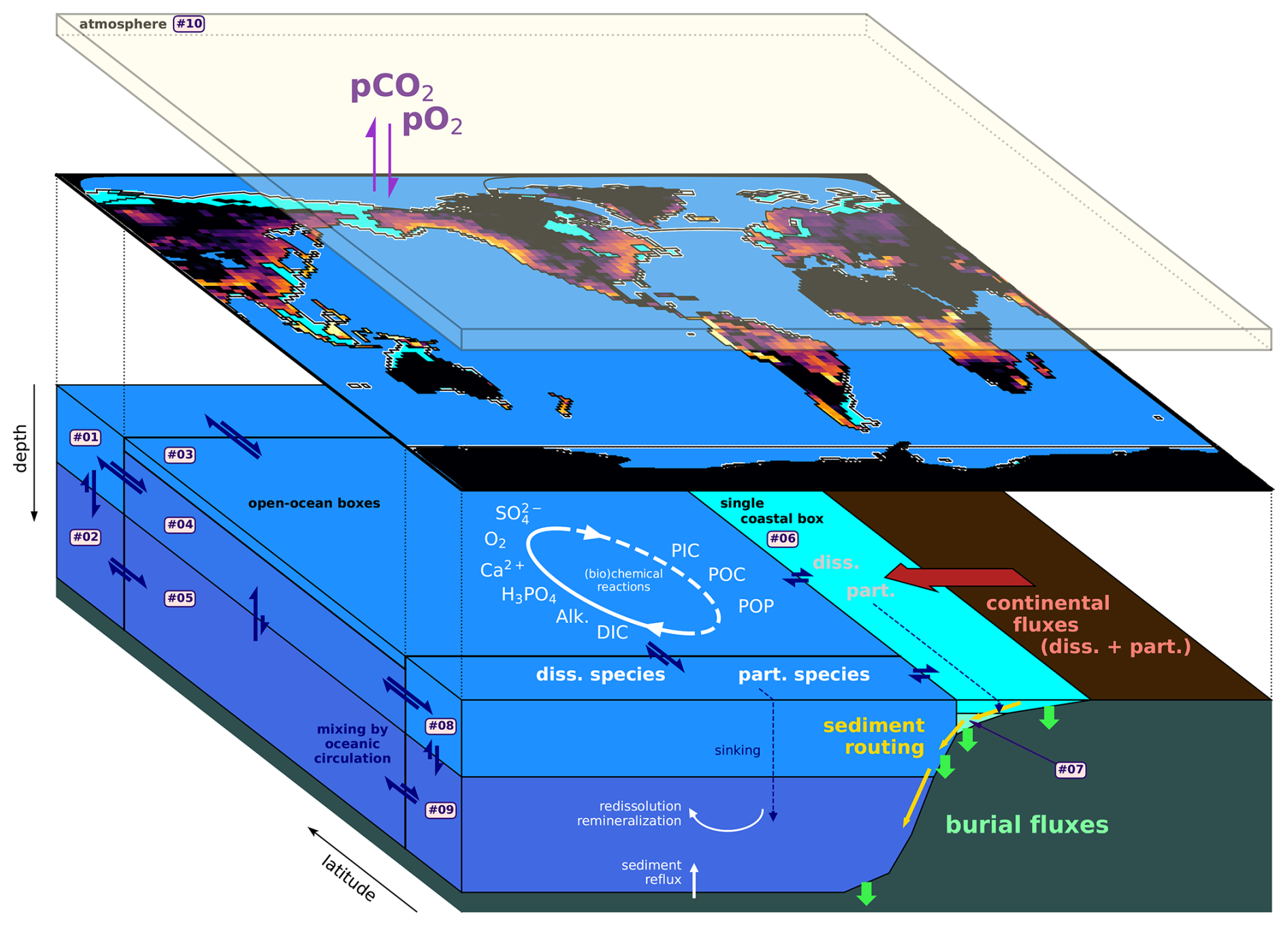
Figure 1 Schematics of the GEOCLIM default 10-box configuration (9 oceanic + 1 atmospheric). The continental discretization is shown by the map of the silicate weathering field. The 10 main GEOCLIM geochemical species (excluding tracers and isotopes) are indicated and their global cycles broadly represented.

In the latest version of GEOCLIM, the definition of the oceanic boxes has been made customizable to better represent any paleogeography. This is one of the most recent improvements. For instance, it is now possible to explicitly represent an isolated basin (e.g., the Mediterranean Sea), or a basin where deepwater formation takes place, to capture key features of the oceanic circulation. This is achieved through the definition of a box (more exactly, a “column” of boxes because of the vertical discretization) for the considered basin. Although customizable, the definition of GEOCLIM boxes should follow a couple of rules: first, oceanic boxes are meant to represent large oceanic basins, with some subgrid-scale parameterizations (e.g., depth of lysocline within the box), and cannot go down to the size of a GCM grid cell. Second, there must be a separation between coastal and open-ocean boxes, with the coastal surface boxes collecting the continental fluxes. This said, there is no constraint on the horizontal splitting of oceanic boxes. Boxes are arranged by “columns”, with no multiple overlap; i.e., there cannot be more than one box immediately below or above a given box. The order of the boxes is also critical: any box i must be immediately below the box i−1, unless box i−1 is at the bottom of the ocean (with no box below), in which case box i must be at the ocean surface (with no box above). There must be exactly four vertical levels intercepting the seafloor: the two coastal levels, followed by the bottom two open-ocean levels. Finally, a single atmospheric box is expected and must be indexed as the last box. Another example of an oceanic box configuration is illustrated Sect. 3, in Fig. 3, for the Turonian paleogeography, with a total of 29 boxes (including the atmosphere).

2.2.2 Mass balance equations

The model computes the temporal evolution of 18 prognostic variables: 8 dissolved or atmospheric species, 4 particulate species, and 6 isotopic variables. All of these variables were already considered in the last published version of GEOCLIM (Maffre et al., 2021), and the mass balance equations are unchanged since this version. In all the following equations, [X] stands for “molar concentration of species X (in mol m⁻³)”. The subscript (i) in the fluxes indicates that they only refer to the box i. For continental fluxes (e.g., the silicate weathering flux ${F_{\text{silw}}}_{\left(i\right)}$), it corresponds to the flux integrated over the continental drainage basin of the oceanic box i. That drainage basin may not exist (if the box i is not coastal), in which case the flux is null. V_i is the volume of ocean box i. $F_{\text{adv}}(\mathrm{X}{)}_{\left(i\right)}^{\text{net}}$ is the net flux of the dissolved species X in the box i resulting from advection (water exchanges) between all the boxes, and $F_{\text{sink}}(\mathrm{Y}{)}_{\left(i\right)}^{\text{net}}$ is the net flux of the particulate species Y in the box i resulting from the vertical sinking of particles. See Sect. 2.2.8 for the derivation of those two fluxes.

Here we describe the mass balance equations for the 12 dissolved, atmospheric, and particulate variables. Depending on the box location (open ocean or coastal; surface, intermediate, or deep), some of the fluxes are set to 0. For instance, the removal of carbon by the precipitation of CaCO₃ in the reefal environment is calculated in the surface water of the coastal boxes and forced to be 0 in the surface boxes of the open oceans and in non-surface boxes.

Total dissolved inorganic carbon (DIC), i.e., ${\mathrm{H}}_{\mathrm{2}}{\mathrm{CO}}_{\mathrm{3}}+{\mathrm{HCO}}_{\mathrm{3}}^{-}+{\mathrm{CO}}_{\mathrm{3}}^{\mathrm{2}-}$. Dissolved CO₂ is assimilated to H₂CO₃.

$$\begin{array}{}\text{(1)}& \begin{array}{rl}{V}_i{\displaystyle \frac{\mathrm{d}[\text{DIC}{]}_{\left(i\right)}}{\mathrm{d}t}}=& -{F_{\text{PP}}^{\text{org}}}_{\left(i\right)}-{F_{\text{PP}}^{\text{inorg}}}_{\left(i\right)}-{F_{\text{reef}}}_{\left(i\right)}\\ & +{F_{\text{diss}}^{\text{PIC}}}_{\left(i\right)}+{F_{\text{remin}}^{\text{POC}}}_{\left(i\right)}+{F_{\text{sed}}^{{\mathrm{CO}}_{\mathrm{2}}}}_{\left(i\right)}\\ & +\mathrm{2}{F_{\text{silw}}}_{\left(i\right)}+\mathrm{2}{F_{\text{carw}}}_{\left(i\right)}+x_{\text{carb}}^{\text{sulw}}{F_{\text{sulw}}}_{\left(i\right)}\\ & +{F_{\text{focw}}}_{\left(i\right)}+{F_{\text{MOR}}^{{\mathrm{CO}}_{\mathrm{2}}}}_{\left(i\right)}-{F_{\mathrm{O}\to \mathrm{A}}^{{\mathrm{CO}}_{\mathrm{2}}}}_{\left(i\right)}\\ & +F_{\text{adv}}(\text{DIC}{)}_{\left(i\right)}^{\text{net}}\end{array}\end{array}$$

Here, $F_{\text{PP}}^{\text{org}}$ is the net primary productivity flux (the biologically produced organic carbon) consuming DIC and transferring the carbon to the reservoir of particulate organic carbon (POC). $F_{\text{PP}}^{\text{inorg}}$ is the net primary productivity flux of particulate inorganic carbon (PIC), i.e., carbonated shells of organisms. F_reef is the flux of carbonate precipitated in reefs (by corals or other bioconstructing organisms, like rudists). $F_{\text{diss}}^{\text{PIC}}$ and $F_{\text{remin}}^{\text{POC}}$ are the fluxes of PIC (POC) that dissolve (remineralize) in the water column. $F_{\text{sed}}^{{\mathrm{CO}}_{\mathrm{2}}}$ is the CO₂ flux from sediment (due to remineralization of organic C during early diagenesis). F_silw, F_carw, F_sulw, and F_focw are the silicate, carbonate, sulfide, and fossil organic carbon weathering fluxes (respectively). $x_{\text{carb}}^{\text{sulw}}$ is the fraction of sulfide weathering associated with carbonate dissolution that actually produces DIC. $F_{\text{MOR}}^{{\mathrm{CO}}_{\mathrm{2}}}$ is the CO₂ degassing from mid-oceanic ridges. ${F_{\mathrm{O}\to \mathrm{A}}^{{\mathrm{CO}}_{\mathrm{2}}}}_{\left(i\right)}$ is the net ocean-to-atmosphere CO₂ exchange in the box i.

Atmospheric CO₂ ($n{{\mathrm{CO}}_{\mathrm{2}}}^{\text{atm}}$ being the molar amount of CO₂ in the atmosphere).

$$\begin{array}{}\text{(2)}& \begin{array}{rl}{\displaystyle \frac{\mathrm{d}\left(n{{\mathrm{CO}}_{\mathrm{2}}}^{\text{atm}}\right)}{\mathrm{d}t}}=& -\mathrm{2}{F}_{\text{silw}}-F_{\text{carw}}-F_{\text{bocx}}+F_{\text{volc}}^{{\mathrm{CO}}_{\mathrm{2}}}\\ & +F_{\text{trap}}^{{\mathrm{CO}}_{\mathrm{2}}}+F_{\text{anth}}^{{\mathrm{CO}}_{\mathrm{2}}}+\sum _i{F_{\mathrm{O}\to \mathrm{A}}^{{\mathrm{CO}}_{\mathrm{2}}}}_{\left(i\right)}\end{array}\end{array}$$

Here, F_bocx is the land-integrated flux of organic carbon produced by vegetation that is exported to the ocean and effectively consumes atmospheric CO₂. $F_{\text{volc}}^{{\mathrm{CO}}_{\mathrm{2}}}$, $F_{\text{trap}}^{{\mathrm{CO}}_{\mathrm{2}}}$, and $F_{\text{anth}}^{{\mathrm{CO}}_{\mathrm{2}}}$ are the CO₂ degassing fluxes from, respectively, subaerial volcanism, trap eruption, and anthropogenic activities. All of them are imposed in the model (i.e., not calculated), but they have been split into three because of their different isotopic signature effects on oxygen (anthropogenic emissions consume O₂) and implementations in the code (constant or temporal scenario). By default, only $F_{\text{volc}}^{{\mathrm{CO}}_{\mathrm{2}}}$ has a nonzero value.

Alkalinity (Alk), approximated as ${\mathrm{HCO}}_{\mathrm{3}}^{-}+\mathrm{2}{\mathrm{CO}}_{\mathrm{3}}^{\mathrm{2}-}+\mathrm{B}(\mathrm{OH}{)}_{\mathrm{4}}^{-}$. Alkalinity is a conservative variable, allowing us to calculate its temporal evolution with a mass balance equation. The approximation is made that only carbonate ion fluxes modify the alkalinity budget (in eq m⁻³).

$$\begin{array}{}\text{(3)}& \begin{array}{rl}{V}_i{\displaystyle \frac{\mathrm{d}[\text{Alk}{]}_{\left(i\right)}}{\mathrm{d}t}}=& -\mathrm{2}{F_{\text{PP}}^{\text{inorg}}}_{\left(i\right)}-\mathrm{2}{F_{\text{reef}}}_{\left(i\right)}+\mathrm{2}{F_{\text{diss}}^{\text{PIC}}}_{\left(i\right)}\\ & +\mathrm{2}{F_{\text{SR}}}_{\left(i\right)}+\mathrm{2}{F_{\text{silw}}}_{\left(i\right)}+\mathrm{2}{F_{\text{carw}}}_{\left(i\right)}\\ & +F_{\text{adv}}(\text{Alk}{)}_{\left(i\right)}^{\text{net}}\end{array}\end{array}$$

Here, 2F_SR is the alkalinity released by the sulfate reduction in marine sediments.

Dissolved phosphate (H₃PO₄).

$$\begin{array}{}\text{(4)}& \begin{array}{rl}{V}_i{\displaystyle \frac{\mathrm{d}[{\mathrm{H}}_{\mathrm{3}}{\mathrm{PO}}_{\mathrm{4}}{]}_{\left(i\right)}}{\mathrm{d}t}}=& -{\displaystyle \frac{\mathrm{1}}{(\mathrm{C}:\mathrm{P}{)}_{\text{Red}}}}{F_{\text{PP}}^{\text{org}}}_{\left(i\right)}\\ & +{\displaystyle \frac{\mathrm{1}}{(\mathrm{C}:\mathrm{P}{)}_{\text{Red}}}}{F_{\text{remin}}^{\text{POC}}}_{\left(i\right)}+{F_{\text{P\hspace{0.17em}sed}}^{\text{net}}}_{\left(i\right)}\\ & +{F_{\text{diss}}^{\mathrm{P}\mathrm{w}}}_{\left(i\right)}+F_{\text{adv}}({\mathrm{H}}_{\mathrm{3}}{\mathrm{PO}}_{\mathrm{4}}{)}_{\left(i\right)}^{\text{net}}\end{array}\end{array}$$

Here, (C:P)_Red is the phosphorus–carbon Redfield ratio, $F_{\mathrm{P}\text{sed}}^{\text{net}}$ is the net sediment-to-ocean phosphorus flux due to early diagenesis processes, and $F_{\text{diss}}^{\mathrm{P}\mathrm{w}}$ is the phosphorus weathering flux (in dissolved form).

Dissolved calcium (Ca²⁺).

$$\begin{array}{}\text{(5)}& \begin{array}{rl}{V}_i{\displaystyle \frac{\mathrm{d}[{\mathrm{Ca}}^{\mathrm{2}+}{]}_{\left(i\right)}}{\mathrm{d}t}}=& -{F_{\text{PP}}^{\text{inorg}}}_{\left(i\right)}-{F_{\text{reef}}}_{\left(i\right)}+{F_{\text{diss}}^{\text{PIC}}}_{\left(i\right)}\\ & +{F_{\text{silw}}}_{\left(i\right)}+{F_{\text{carw}}}_{\left(i\right)}+{F_{\text{sulw}}}_{\left(i\right)}\\ & +F_{\text{adv}}({\mathrm{Ca}}^{\mathrm{2}+}{)}_{\left(i\right)}^{\text{net}}\end{array}\end{array}$$

Dissolved and atmospheric oxygen (O₂), ($n{{\mathrm{O}}_{\mathrm{2}}}^{\text{atm}}$ being the molar amount of O₂ in the atmosphere).

$$\begin{array}{}\text{(6)}& {\displaystyle }\begin{array}{rl}{V}_i{\displaystyle \frac{\mathrm{d}[{\mathrm{O}}_{\mathrm{2}}{]}_{\left(i\right)}}{\mathrm{d}t}}=& {F_{\text{PP}}^{\text{org}}}_{\left(i\right)}-{F_{\text{remin}}^{\text{POC}}}_{\left(i\right)}-{F_{\text{sed}}^{{\mathrm{O}}_{\mathrm{2}}}}_{\left(i\right)}\\ & -{F_{\mathrm{O}\to \mathrm{A}}^{{\mathrm{O}}_{\mathrm{2}}}}_{\left(i\right)}+F_{\text{adv}}({\mathrm{O}}_{\mathrm{2}}{)}_{\left(i\right)}^{\text{net}}\end{array}\text{(7)}& {\displaystyle }\begin{array}{rl}{\displaystyle \frac{\mathrm{d}\left(n{{\mathrm{O}}_{\mathrm{2}}}^{\text{atm}}\right)}{\mathrm{d}t}}=& F_{\text{bocx}}-F_{\text{focw}}-{\displaystyle \frac{\mathrm{15}}{\mathrm{8}}}{F}_{\text{sulw}}\\ & +\sum _i{F_{\mathrm{O}\to \mathrm{A}}^{{\mathrm{O}}_{\mathrm{2}}}}_{\left(i\right)}-F_{\text{anth}}^{{\mathrm{CO}}_{\mathrm{2}}}\end{array}\end{array}$$

Here, $F_{\text{sed}}^{{\mathrm{O}}_{\mathrm{2}}}$ is the oxygen consumption by all early diagenesis processes. $F_{\mathrm{O}\to \mathrm{A}}^{{\mathrm{O}}_{\mathrm{2}}}$ is the net ocean-to-atmosphere oxygen exchange. The factor $\frac{\mathrm{15}}{\mathrm{8}}$ comes from the stoichiometry of sulfide weathering equation.

Dissolved sulfate (${\mathrm{SO}}_{\mathrm{4}}^{\mathrm{2}-}$).

$$\begin{array}{}\text{(8)}& V_i{\displaystyle \frac{\mathrm{d}[{\mathrm{SO}}_{\mathrm{4}}^{\mathrm{2}-}{]}_{\left(i\right)}}{\mathrm{d}t}}={F_{\text{sulw}}}_{\left(i\right)}-{F_{\text{SR}}}_{\left(i\right)}+F_{\text{adv}}({\mathrm{SO}}_{\mathrm{4}}^{\mathrm{2}-}{)}_{\left(i\right)}^{\text{net}}\end{array}$$

Particulate inorganic carbon (PIC).

$$\begin{array}{}\text{(9)}& V_i{\displaystyle \frac{\mathrm{d}[\text{PIC}{]}_{\left(i\right)}}{\mathrm{d}t}}={F_{\text{PP}}^{\text{inorg}}}_{\left(i\right)}-{F_{\text{diss}}^{\text{PIC}}}_{\left(i\right)}+F_{\text{sink}}(\text{PIC}{)}_{\left(i\right)}^{\text{net}}\end{array}$$

Particulate organic carbon (POC).

$$\begin{array}{}\text{(10)}& \begin{array}{rl}{V}_i{\displaystyle \frac{\mathrm{d}[\text{POC}{]}_{\left(i\right)}}{\mathrm{d}t}}=& {F_{\text{PP}}^{\text{org}}}_{\left(i\right)}-{F_{\text{remin}}^{\text{POC}}}_{\left(i\right)}\\ & +F_{\text{bocx}}+F_{\text{sink}}(\text{POC}{)}_{\left(i\right)}^{\text{net}}\end{array}\end{array}$$

Particulate organic phosphorus (POP), i.e., phosphorus associated with POC.

$$\begin{array}{}\text{(11)}& \begin{array}{rl}{V}_i{\displaystyle \frac{\mathrm{d}[\text{POP}{]}_{\left(i\right)}}{\mathrm{d}t}}=& {\displaystyle \frac{\mathrm{1}}{(\mathrm{C}:\mathrm{P}{)}_{\text{Red}}}}{F_{\text{PP}}^{\text{org}}}_{\left(i\right)}-{\displaystyle \frac{[\text{POP}{]}_{\left(i\right)}}{[\text{POC}{]}_{\left(i\right)}}}{F_{\text{remin}}^{\text{POC}}}_{\left(i\right)}\\ & +{F_{\text{part}}^{\mathrm{P}\mathrm{w}}}_{\left(i\right)}+F_{\text{sink}}(\text{POP}{)}_{\left(i\right)}^{\text{net}}\end{array}\end{array}$$

Here, $F_{\text{part}}^{\mathrm{P}\mathrm{w}}$ is the phosphorus weathering flux in particulate form.

The following species (dissolved Sr and Sr associated with PIC) are tracers. Tracers are prognostic geochemical variables (i.e., variables whose temporal evolutions are explicitly computed by solving their differential equations), whose evolution has strictly no influence on the other main geochemical species.

Dissolved strontium.

$$\begin{array}{}\text{(12)}& {\displaystyle }\begin{array}{rl}{V}_i{\displaystyle \frac{\mathrm{d}[\mathrm{Sr}{]}_{\left(i\right)}}{\mathrm{d}t}}=& -{r_{\text{PIC}}^{\mathrm{Sr}}}_{\left(i\right)}({F_{\text{PP}}^{\text{inorg}}}_{\left(i\right)}+{F_{\text{reef}}}_{\left(i\right)})\\ & +{\displaystyle \frac{[{\mathrm{Sr}}_{\text{PIC}}{]}_{\left(i\right)}}{[\text{PIC}{]}_{\left(i\right)}}}{F_{\text{diss}}^{\text{PIC}}}_{\left(i\right)}\\ & +r_{\text{sil}}^{\mathrm{Sr}}({F_{\text{silw}}}_{\left(i\right)}+x_{\text{sil}}^{\text{sulw}}{F_{\text{sulw}}}_{\left(i\right)})\\ & +r_{\text{carb}}^{\mathrm{Sr}}({F_{\text{carw}}}_{\left(i\right)}+x_{\text{carb}}^{\text{sulw}}{F_{\text{sulw}}}_{\left(i\right)})\\ & +F_{\text{adv}}(\mathrm{Sr}{)}_{\left(i\right)}^{\text{net}}\end{array}\end{array}$$

Here, $r_{\text{sil}}^{\mathrm{Sr}}$, $r_{\text{carb}}^{\mathrm{Sr}}$, and $r_{\text{PIC}}^{\mathrm{Sr}}$ are, respectively, the Sr:CaMg ratio in weathered silicate minerals, the Sr:Ca ratio in weathered carbonate minerals, and the Sr:Ca ratio in biologically precipitated oceanic carbonate. For the sake of simplicity, that last ratio ($r_{\text{PIC}}^{\mathrm{Sr}}$) is assumed to be the same for all shells and for reefs. $r_{\text{PIC}}^{\mathrm{Sr}}$ is also assumed to be dependent on seawater Sr concentration, thus stabilizing the Sr cycle:

$$\begin{array}{}\text{(13)}& {r_{\text{PIC}}^{\mathrm{Sr}}}_{\left(i\right)}=(\mathrm{0.72}{r}_{\text{sil}}^{\mathrm{Sr}}+\mathrm{0.28}{r}_{\text{carb}}^{\mathrm{Sr}}){\displaystyle \frac{[\mathrm{Sr}{]}_{\left(i\right)}}{[\mathrm{Sr}{]}_{\text{ref}}}},\end{array}$$

with [Sr]_ref being the pre-industrial mean Sr concentration. Equation (13) should be seen as a tuning equation: given that the proportion of Sr input from the ocean is approximately 72 % from silicate weathering and 28 % from carbonate weathering, setting the Sr:C ratio of PIC this way ensures that the mean oceanic Sr concentration at which the carbonate burial Sr sink balance the input fluxes is [Sr]_ref.

PIC from strontium incorporated in carbonate shells.

$$\begin{array}{}\text{(14)}& \begin{array}{rl}{V}_i{\displaystyle \frac{\mathrm{d}[{\mathrm{Sr}}_{\text{PIC}}{]}_{\left(i\right)}}{\mathrm{d}t}}=& r_{{\text{PIC}}_{\left(i\right)}}^{\mathrm{Sr}}{F_{\text{PP}}^{\text{inorg}}}_{\left(i\right)}-{\displaystyle \frac{[{\mathrm{Sr}}_{\text{PIC}}{]}_{\left(i\right)}}{[\text{PIC}{]}_{\left(i\right)}}}{F_{\text{diss}}^{\text{PIC}}}_{\left(i\right)}\\ & +F_{\text{sink}}({\mathrm{Sr}}_{\text{PIC}}{)}_{\left(i\right)}^{\text{net}}\end{array}\end{array}$$

2.2.3 Isotopic mass balance equations

The isotopic tracer and mass balance equations presented here are also unchanged since Maffre et al. (2021). All of these isotopic mass balance equations follow the classical formulation, with X being an element and δⁿX its isotopic composition (where the notation δ represents the difference between the concerned isotopic ratio and a standard, normalized by the standard and multiplied by 1000):

$$\begin{array}{}\text{(15)}& V_i[\mathrm{X}{]}_{\left(i\right)}{\displaystyle \frac{\mathrm{d}\left(\mathit{\delta }{{}^{\mathrm{n}}\mathrm{X}}_{\left(i\right)}\right)}{\mathrm{d}t}}=\sum \text{Flux}(\mathrm{X}{)}_{\left(i\right)}\left(\mathit{\delta }{{}^{\mathrm{n}}\mathrm{X}}_{\text{flux}}-\mathit{\delta }{{}^{\mathrm{n}}\mathrm{X}}_{\left(i\right)}\right),\end{array}$$

where $\mathit{\delta }{{}^{\mathrm{n}}\mathrm{X}}_{\text{flux}}$ is the isotopic signature associated with the given flux. All the isotopic fluxes fall within the generic form in the right half of Eq. (15), including the net isotopic flux of X in box i due to water exchanges (if X is a dissolved species), denoted as $F_{\text{adv}}(\mathit{\delta }{}^{\mathrm{n}}\mathrm{X}{)}_{\left(i\right)}^{\text{net}}$, and the net isotopic flux of Y in box i due to vertical particle sinking (if Y is a particulate species), denoted as $F_{\text{sink}}(\mathit{\delta }{}^{\mathrm{n}}\mathrm{Y}{)}_{\left(i\right)}^{\text{net}}$. The computation of those fluxes is detailed Sect. 2.2.11.

The strontium isotopic equations, however, are treated differently, using the atomic fraction of ⁸⁷Sr (that includes other isotopes than ⁸⁷Sr and ⁸⁶Sr) expressed as a function of ${}^{\mathrm{87}}\mathrm{Sr}{/}^{\mathrm{86}}\mathrm{Sr}$ (François and Walker, 1992; Li and Elderfield, 2013).

$$\begin{array}{}\text{(16)}& \begin{array}{rl}{V}_i& {\displaystyle \frac{[\mathrm{Sr}{]}_{\left(i\right)}}{\mathrm{9.43}+\mathit{\{}{}^{\mathrm{87}}\mathrm{Sr}{/}^{\mathrm{86}}\mathrm{Sr}{\mathit{\}}}_{\left(i\right)}}}{\displaystyle \frac{\mathrm{d}\left(\mathit{\right\{}{}^{\mathrm{87}}\mathrm{Sr}{/}^{\mathrm{86}}\mathrm{Sr}{\mathit{\}}}_{\left(i\right)})}{\mathrm{d}t}}=\\ & \sum \text{Flux}(\mathrm{Sr}{)}_{\left(i\right)}{\displaystyle \frac{\mathit{\{}{}^{\mathrm{87}}\mathrm{Sr}{/}^{\mathrm{86}}\mathrm{Sr}{\mathit{\}}}_{\text{flux}}-\mathit{\{}{}^{\mathrm{87}}\mathrm{Sr}{/}^{\mathrm{86}}\mathrm{Sr}{\mathit{\}}}_{\left(i\right)}}{\mathrm{9.43}+\mathit{\{}{}^{\mathrm{87}}\mathrm{Sr}{/}^{\mathrm{86}}\mathrm{Sr}{\mathit{\}}}_{\text{flux}}}}\end{array}\end{array}$$

For the sake of readability, we denote “σ_⋆” the isotopic ratio $\mathit{\{}{}^{\mathrm{87}}\mathrm{Sr}{/}^{\mathrm{86}}\mathrm{Sr}{\mathit{\}}}_{\star }$. Hence, σ_carb and σ_sil are the Sr isotopic ratios of weathered carbonate and silicate (respectively), while σ_d and σ_p are the Sr isotopic ratios of oceanic dissolved Sr and Sr associated with PIC (respectively). The net advective or sinking isotopic flux of Sr also falls within the generic form in the right half of Eq. (16) and are denoted $F_{\text{adv}}({\mathit{\sigma }}_{\star }{)}_{\left(i\right)}^{\text{net}}$ and $F_{\text{sink}}({\mathit{\sigma }}_{\star }{)}_{\left(i\right)}^{\text{net}}$.

${}^{\mathrm{87}}\mathrm{Sr}{/}^{\mathrm{86}}\mathrm{Sr}$ ratio of dissolved strontium (σ_d).

$$\begin{array}{}\text{(17)}& {\displaystyle }\begin{array}{rl}{V}_i& {\displaystyle \frac{[\mathrm{Sr}{]}_{\left(i\right)}}{\mathrm{9.43}+{{\mathit{\sigma }}_{\mathrm{d}}}_{\left(i\right)}}}{\displaystyle \frac{\mathrm{d}\left({{\mathit{\sigma }}_{\mathrm{d}}}_{\left(i\right)}\right)}{\mathrm{d}t}}=\\ & +{\displaystyle \frac{[{\mathrm{Sr}}_{\text{PIC}}{]}_{\left(i\right)}}{[\text{PIC}{]}_{\left(i\right)}}}{F_{\text{diss}}^{\text{PIC}}}_{\left(i\right)}{\displaystyle \frac{{{\mathit{\sigma }}_{\mathrm{p}}}_{\left(i\right)}-{{\mathit{\sigma }}_{\mathrm{d}}}_{\left(i\right)}}{\mathrm{9.43}+{{\mathit{\sigma }}_{\mathrm{p}}}_{\left(i\right)}}}\\ & +r_{\text{sil}}^{\mathrm{Sr}}({F_{\text{silw}}}_{\left(i\right)}+x_{\text{sil}}^{\text{sulw}}{F_{\text{sulw}}}_{\left(i\right)}){\displaystyle \frac{\stackrel{\mathrm{‾}}{{{\mathit{\sigma }}_{\text{sil}}}_{\left(i\right)}}-{{\mathit{\sigma }}_{\mathrm{d}}}_{\left(i\right)}}{\mathrm{9.43}+\stackrel{\mathrm{‾}}{{{\mathit{\sigma }}_{\text{sil}}}_{\left(i\right)}}}}\\ & +r_{\text{carb}}^{\mathrm{Sr}}({F_{\text{carw}}}_{\left(i\right)}+x_{\text{carb}}^{\text{sulw}}{F_{\text{sulw}}}_{\left(i\right)}){\displaystyle \frac{{\mathit{\sigma }}_{\text{carb}}-{{\mathit{\sigma }}_{\mathrm{d}}}_{\left(i\right)}}{\mathrm{9.43}+{\mathit{\sigma }}_{\text{carb}}}}\\ & +r_{\text{MOR}}^{\mathrm{Sr}}{F_{\text{MOR}}^{{\mathrm{CO}}_{\mathrm{2}}}}_{\left(i\right)}{\displaystyle \frac{{\mathit{\sigma }}_{\text{MOR}}-{{\mathit{\sigma }}_{\mathrm{d}}}_{\left(i\right)}}{\mathrm{9.43}+{\mathit{\sigma }}_{\text{MOR}}}}\\ & +F_{\text{adv}}({\mathit{\sigma }}_{\mathrm{d}}{)}_{\left(i\right)}^{\text{net}}\end{array}\end{array}$$

Here, $\stackrel{\mathrm{‾}}{{{\mathit{\sigma }}_{\text{sil}}}_{\left(i\right)}}$ is the averaged Sr isotopic ratio from silicate weathering delivered to box i, weighted by the relative contribution of each lithology to silicate weathering, since each lithology has a specific Sr isotopic ratio. σ_carb is the Sr isotopic ratio in continental carbonate (assumed to be constant), σ_MOR is the mantle Sr isotopic ratio, and $r_{\text{MOR}}^{\mathrm{Sr}}$ is the ratio between the exchanged Sr flux and the degassed CO₂ flux at mid-ocean ridges. Note that $r_{\text{MOR}}^{\mathrm{Sr}}{F_{\text{MOR}}^{{\mathrm{CO}}_{\mathrm{2}}}}_{\left(i\right)}$ does not contribute to the Sr budget (Eq. 12) since it is an Sr exchange (i.e., null net flux), but it affects the isotopic composition. PIC precipitation does not affect the Sr isotopic budget of any box, since there is no fractionation associated with Sr incorporation in PIC, but PIC dissolution does affect the Sr isotopic budget because PIC dissolving in the box i may have a different isotopic ratio than the surrounding water.

${}^{\mathrm{87}}\mathrm{Sr}{/}^{\mathrm{86}}\mathrm{Sr}$ ratio of strontium associated with PIC (σ_p).

$$\begin{array}{}\text{(18)}& \begin{array}{rl}{V}_i& {\displaystyle \frac{[{\mathrm{Sr}}_{\text{PIC}}{]}_{\left(i\right)}}{\mathrm{9.43}+{{\mathit{\sigma }}_{\mathrm{p}}}_{\left(i\right)}}}{\displaystyle \frac{\mathrm{d}\left({{\mathit{\sigma }}_{\mathrm{p}}}_{\left(i\right)}\right)}{\mathrm{d}t}}=\\ & +{r_{\text{PIC}}^{\mathrm{Sr}}}_{\left(i\right)}{F_{\text{PP}}^{\text{inorg}}}_{\left(i\right)}{\displaystyle \frac{{{\mathit{\sigma }}_{\mathrm{d}}}_{\left(i\right)}-{{\mathit{\sigma }}_{\mathrm{p}}}_{\left(i\right)}}{\mathrm{9.43}+{{\mathit{\sigma }}_{\mathrm{d}}}_{\left(i\right)}}}+F_{\text{sink}}({\mathit{\sigma }}_{\mathrm{p}}{)}_{\left(i\right)}^{\text{net}}\end{array}\end{array}$$

DIC δ¹³C.

$$\begin{array}{}\text{(19)}& \begin{array}{rl}{V}_i& [\text{DIC}{]}_{\left(i\right)}{\displaystyle \frac{\mathrm{d}\left(\mathit{\delta }{{{}^{\mathrm{13}}\mathrm{C}}_{\text{DIC}}}_{\left(i\right)}\right)}{\mathrm{d}t}}=\\ & -{F_{\text{PP}}^{\text{org}}}_{\left(i\right)}(\mathit{\delta }{{{}^{\mathrm{13}}\mathrm{C}}_{{\mathrm{H}}_{\mathrm{2}}{\mathrm{CO}}_{\mathrm{3}}}}_{\left(i\right)}-{{\mathit{ϵ}}_{\text{PP}}}_{\left(i\right)}-\mathit{\delta }{{{}^{\mathrm{13}}\mathrm{C}}_{\text{DIC}}}_{\left(i\right)})\\ & -({F_{\text{PP}}^{\text{inorg}}}_{\left(i\right)}+{F_{\text{reef}}}_{\left(i\right)})(\mathit{\delta }{{{}^{\mathrm{13}}\mathrm{C}}_{{\mathrm{CO}}_{\mathrm{3}}^{\mathrm{2}-}}}_{\left(i\right)}-\mathit{\delta }{{{}^{\mathrm{13}}\mathrm{C}}_{\text{DIC}}}_{\left(i\right)})\\ & +{F_{\text{diss}}^{\text{PIC}}}_{\left(i\right)}(\mathit{\delta }{{{}^{\mathrm{13}}\mathrm{C}}_{\text{PIC}}}_{\left(i\right)}-\mathit{\delta }{{{}^{\mathrm{13}}\mathrm{C}}_{\text{DIC}}}_{\left(i\right)})\\ & +({F_{\text{remin}}^{\text{POC}}}_{\left(i\right)}+{F_{\text{sed}}^{{\mathrm{CO}}_{\mathrm{2}}}}_{\left(i\right)})(\mathit{\delta }{{{}^{\mathrm{13}}\mathrm{C}}_{\text{POC}}}_{\left(i\right)}-\mathit{\delta }{{{}^{\mathrm{13}}\mathrm{C}}_{\text{DIC}}}_{\left(i\right)})\\ & +(\mathrm{2}{F_{\text{silw}}}_{\left(i\right)}+{F_{\text{carw}}}_{\left(i\right)})(\mathit{\delta }{{}^{\mathrm{13}}\mathrm{C}}_{{\mathrm{CO}}_{\mathrm{2}}}^{\text{atm}}-\mathit{\delta }{{{}^{\mathrm{13}}\mathrm{C}}_{\text{DIC}}}_{\left(i\right)})\\ & +({F_{\text{carw}}}_{\left(i\right)}+x_{\text{carb}}^{\text{sulw}}{F_{\text{sulw}}}_{\left(i\right)})(\mathit{\delta }{{}^{\mathrm{13}}\mathrm{C}}_{\text{carb}}-\mathit{\delta }{{{}^{\mathrm{13}}\mathrm{C}}_{\text{DIC}}}_{\left(i\right)})\\ & +{F_{\text{focw}}}_{\left(i\right)}(\mathit{\delta }{{}^{\mathrm{13}}\mathrm{C}}_{\text{foc}}-\mathit{\delta }{{{}^{\mathrm{13}}\mathrm{C}}_{\text{DIC}}}_{\left(i\right)})\\ & +{F_{\text{MOR}}^{{\mathrm{CO}}_{\mathrm{2}}}}_{\left(i\right)}(\mathit{\delta }{{}^{\mathrm{13}}\mathrm{C}}_{\text{MOR}}-\mathit{\delta }{{{}^{\mathrm{13}}\mathrm{C}}_{\text{DIC}}}_{\left(i\right)})\\ & +F_{A\to \left(i\right)}^{{\mathrm{CO}}_{\mathrm{2}}{\mathit{\delta }}^{\mathrm{13}}\mathrm{C}}+F_{\text{adv}}(\mathit{\delta }{{}^{\mathrm{13}}\mathrm{C}}_{\text{DIC}}{)}_{\left(i\right)}^{\text{net}}\end{array}\end{array}$$

Here, $\mathit{\delta }{{}^{\mathrm{13}}\mathrm{C}}_{\text{carb}}$, $\mathit{\delta }{{}^{\mathrm{13}}\mathrm{C}}_{\text{foc}}$, and $\mathit{\delta }{{}^{\mathrm{13}}\mathrm{C}}_{\text{MOR}}$ are the C isotopic compositions of continental carbonates, petrogenic organic carbon, and mid-ocean ridge CO₂ (respectively). ${{\mathit{ϵ}}_{\text{PP}}}_{\left(i\right)}$ is the isotopic fractionation associated with oceanic photosynthesis that consumes H₂CO₃. Therefore, the isotopic composition of marine organic matter is $\mathit{\delta }{{{}^{\mathrm{13}}\mathrm{C}}_{{\mathrm{H}}_{\mathrm{2}}{\mathrm{CO}}_{\mathrm{3}}}}_{\left(i\right)}-{{\mathit{ϵ}}_{\text{PP}}}_{\left(i\right)}$. Similarly, the PIC precipitation flux takes dissolved inorganic carbon as ${\mathrm{CO}}_{\mathrm{3}}^{\mathrm{2}-}$, without fractionation. $F_{\mathrm{A}\to \left(i\right)}^{{\mathrm{CO}}_{\mathrm{2}}\mathit{\delta }{}^{\mathrm{13}}\mathrm{C}}$ is the net C isotopic flux from the atmosphere to oceanic box i.

lδ¹3C of atmospheric CO₂.

$$\begin{array}{}\text{(20)}& \begin{array}{rl}n& {{\mathrm{CO}}_{\mathrm{2}}}^{\text{atm}}{\displaystyle \frac{\mathrm{d}\left(\mathit{\delta }{{}^{\mathrm{13}}\mathrm{C}}_{{\mathrm{CO}}_{\mathrm{2}}}^{\text{atm}}\right)}{\mathrm{d}t}}=\\ & -F_{\text{bocx}}{\mathit{ϵ}}_{\text{cont}}+F_{\text{volc}}^{{\mathrm{CO}}_{\mathrm{2}}}(\mathit{\delta }{{}^{\mathrm{13}}\mathrm{C}}_{\text{volc}}-\mathit{\delta }{{}^{\mathrm{13}}\mathrm{C}}_{{\mathrm{CO}}_{\mathrm{2}}}^{\text{atm}})\\ & +F_{\text{trap}}^{{\mathrm{CO}}_{\mathrm{2}}}(\mathit{\delta }{{}^{\mathrm{13}}\mathrm{C}}_{\text{trap}}-\mathit{\delta }{{}^{\mathrm{13}}\mathrm{C}}_{{\mathrm{CO}}_{\mathrm{2}}}^{\text{atm}})\\ & +F_{\text{anth}}^{{\mathrm{CO}}_{\mathrm{2}}}(\mathit{\delta }{{}^{\mathrm{13}}\mathrm{C}}_{\text{foc}}-\mathit{\delta }{{}^{\mathrm{13}}\mathrm{C}}_{{\mathrm{CO}}_{\mathrm{2}}}^{\text{atm}})+\sum _i{F}_{\left(i\right)\to \mathrm{A}}^{{\mathrm{CO}}_{\mathrm{2}}{\mathit{\delta }}^{\mathrm{13}}\mathrm{C}}\end{array}\end{array}$$

Here, $\mathit{\delta }{{}^{\mathrm{13}}\mathrm{C}}_{\text{volc}}$ and $\mathit{\delta }{{}^{\mathrm{13}}\mathrm{C}}_{\text{trap}}$ are the δ¹³C of CO₂ degassed by subaerial volcanism and by trap volcanism (respectively). ϵ_cont is the isotopic fractionation associated with continental photosynthesis that consumes atmospheric CO₂. Therefore, the isotopic composition of continental organic matter is $\mathit{\delta }{{}^{\mathrm{13}}\mathrm{C}}_{{\mathrm{CO}}_{\mathrm{2}}}^{\text{atm}}-{\mathit{ϵ}}_{\text{cont}}$. $F_{\left(i\right)\to \mathrm{A}}^{{\mathrm{CO}}_{\mathrm{2}}\mathit{\delta }{}^{\mathrm{13}}\mathrm{C}}$ is the net C isotopic flux from oceanic box i to the atmosphere.

PIC δ¹³C.

$$\begin{array}{}\text{(21)}& \begin{array}{rl}{V}_i& [\text{PIC}{]}_{\left(i\right)}{\displaystyle \frac{\mathrm{d}\left(\mathit{\delta }{{{}^{\mathrm{13}}\mathrm{C}}_{\text{PIC}}}_{\left(i\right)}\right)}{\mathrm{d}t}}=\\ & {F_{\text{PP}}^{\text{inorg}}}_{\left(i\right)}(\mathit{\delta }{{{}^{\mathrm{13}}\mathrm{C}}_{{\mathrm{CO}}_{\mathrm{3}}^{\mathrm{2}-}}}_{\left(i\right)}-\mathit{\delta }{{{}^{\mathrm{13}}\mathrm{C}}_{\text{PIC}}}_{\left(i\right)})\\ & +F_{\text{sink}}(\mathit{\delta }{{}^{\mathrm{13}}\mathrm{C}}_{\text{PIC}}{)}_{\left(i\right)}^{\text{net}}\end{array}\end{array}$$

POC δ¹³C.

$$\begin{array}{}\text{(22)}& \begin{array}{rl}{V}_i& [\text{POC}{]}_{\left(i\right)}{\displaystyle \frac{\mathrm{d}\left(\mathit{\delta }{{{}^{\mathrm{13}}\mathrm{C}}_{\text{POC}}}_{\left(i\right)}\right)}{\mathrm{d}t}}=\\ & {F_{\text{PP}}^{\text{org}}}_{\left(i\right)}(\mathit{\delta }{{{}^{\mathrm{13}}\mathrm{C}}_{{\mathrm{H}}_{\mathrm{2}}{\mathrm{CO}}_{\mathrm{3}}}}_{\left(i\right)}-{{\mathit{ϵ}}_{\text{PP}}}_{\left(i\right)}-\mathit{\delta }{{{}^{\mathrm{13}}\mathrm{C}}_{\text{POC}}}_{\left(i\right)})\\ & +F_{\text{bocx}}(\mathit{\delta }{{}^{\mathrm{13}}\mathrm{C}}_{{\mathrm{CO}}_{\mathrm{2}}}^{\text{atm}}-{\mathit{ϵ}}_{\text{cont}}-\mathit{\delta }{{{}^{\mathrm{13}}\mathrm{C}}_{\text{POC}}}_{\left(i\right)})\\ & +F_{\text{sink}}(\mathit{\delta }{{}^{\mathrm{13}}\mathrm{C}}_{\text{POC}}{)}_{\left(i\right)}^{\text{net}}\end{array}\end{array}$$

The following sections (2.2.4–2.2.11) describe the computation of the fluxes involved in the mass balance equations.

2.2.4 Primary productivity (particulate inorganic and organic carbon)

The calculation scheme for organic primary productivity was introduced in Goddéris and Joachimski (2004). So was the functional form of reefal carbonate precipitation, although the “modern” (as opposed to the Paleozoic) form was published in Donnadieu et al. (2006), who also introduced the pelagic calcareous productivity.

Primary productivity is computed assuming that phosphorus is the unique limiting nutrient at the geological timescale (Benitez-Nelson, 2000). The primary productivity flux computed by GEOCLIM ($F_{\text{PP}}^{\text{org}}$) represents the net primary productivity of the photic zone, already including biotic interactions and respiration. $F_{\text{PP}}^{\text{org}}$ is calculated as a function of the P input flux in the photic zone and not of the concentration of P within the photic zone. This dependence implies that higher fluxes of dissolved phosphorus entering one of the photic reservoirs (for instance through upwelling) trigger a higher primary productivity associated with a low phosphorus concentration, in line with observations. Hence, for each surface oceanic box i, the net primary productivity is computed as

$$\begin{array}{}\text{(23)}& {F_{\text{PP}}^{\text{org}}}_{\left(i\right)}={r_{\text{eff}}}_{\left(i\right)}(\mathrm{C}:\mathrm{P}{)}_{\text{Red}}\left({F_{\text{diss}}^{\mathrm{P}\mathrm{w}}}_{\left(i\right)}+F_{\text{adv}}({\mathrm{H}}_{\mathrm{3}}{\mathrm{PO}}_{\mathrm{4}}{)}_{\left(i\right)}^{\text{in}}\right),\end{array}$$

where $F_{\text{adv}}({\mathrm{H}}_{\mathrm{3}}{\mathrm{PO}}_{\mathrm{4}}{)}_{\left(i\right)}^{\text{in}}$ is the sum of incoming dissolved phosphorus (H₃PO₄) into the box i by seawater advection and, for coastal boxes, the discharge of dissolved phosphorus from continental weathering. (C:P)_Red is the Redfield ratio. ${r_{\text{eff}}}_{\left(i\right)}$ is an efficiency coefficient that depends on dissolved CO₂, computed as follows.

$$\begin{array}{}\text{(24)}& {r_{\text{eff}}}_{\left(i\right)}=\left\{\begin{array}{ll}max\left(\mathrm{0},\frac{p{{\mathrm{CO}}_{\mathrm{2}}}_{\left(i\right)}^{\text{diss}}/{\left.p{{\mathrm{CO}}_{\mathrm{2}}}^{\text{atm}}\right|}_{\text{PI}}-\mathrm{0.2}}{p{{\mathrm{CO}}_{\mathrm{2}}}_{\left(i\right)}^{\text{diss}}/{\left.p{{\mathrm{CO}}_{\mathrm{2}}}^{\text{atm}}\right|}_{\text{PI}}-\mathrm{0.1}}\right)& \\ & \mathrm{\text{if box }}i\text{ is not polar}\\ max\left(\mathrm{0},\frac{p{{\mathrm{CO}}_{\mathrm{2}}}_{\left(i\right)}^{\text{diss}}/{\left.p{{\mathrm{CO}}_{\mathrm{2}}}^{\text{atm}}\right|}_{\text{PI}}-\mathrm{0.2}}{p{{\mathrm{CO}}_{\mathrm{2}}}_{\left(i\right)}^{\text{diss}}/{\left.p{{\mathrm{CO}}_{\mathrm{2}}}^{\text{atm}}\right|}_{\text{PI}}-\mathrm{0.1}}\right)/\mathrm{3}& \\ & \mathrm{\text{if box }}i\text{ is polar}\end{array}\right.\end{array}$$

Here, $p{{\mathrm{CO}}_{\mathrm{2}}}^{\text{diss}}$ is the partial pressure of dissolved CO₂ (see Eq. 38) and ${\left.p{{\mathrm{CO}}_{\mathrm{2}}}^{\text{atm}}\right|}_{\text{PI}}$ is pre-industrial partial pressure of CO₂. The role of these coefficients is to prevent the depletion of ocean carbon as a result of excessive primary productivity. In all the GEOCLIM simulations carried out since 2004, this limit has never been reached. These coefficients therefore have little effect on the results and should be considered safeguards against overconsumption of dissolved carbon. The division by 3 in polar oceanic boxes represents the light limitation at high latitudes. It was adjusted through model calibration on the present-day world, with the generic 10-box configuration.

The flux of biologically precipitated carbonates in a pelagic environment is scaled to the primary productivity flux $F_{\text{PP}}^{\text{org}}$ and also represents the net flux of the photic zone.

$$\begin{array}{}\text{(25)}& {F_{\text{PP}}^{\text{inorg}}}_{\left(i\right)}=\left\{\begin{array}{ll}\mathrm{0}& \text{if }\mathrm{\Omega }<\mathrm{1}\\ {x_{\text{shell}}}_{\left(i\right)}\frac{{\mathrm{\Omega }}_{\left(i\right)}-\mathrm{1}}{\mathrm{0.4}+{\mathrm{\Omega }}_{\left(i\right)}-\mathrm{1}}{F_{\text{PP}}^{\text{org}}}_{\left(i\right)}& \text{otherwise}\end{array}\right.\end{array}$$

Here, Ω is the saturation ratio with respect to calcite. The scaling coefficient x_shell encompasses the proportion of calcifying primary producers and their inorganic $/$ organic C ratio. Its value is set to 0.15 in open-ocean boxes and 0.015 in coastal boxes. This 10-fold reduction in coastal boxes was tuned in order to avoid massive precipitation of carbonates in coastal surface boxes – given the intensity of primary productivity in those boxes – that would never dissolve (because surface waters are always saturated with respect to the carbonate minerals). The proportion of biologically produced PIC that is aragonitic is the same in all surface reservoirs and is set by the parameter x_arag, equal to 0.396.

The last biologically mediated flux is the precipitation of carbonate in the form of reefs F_reef. For each coastal surface box i, it is computed as follows.

$$\begin{array}{}\text{(26)}& {F_{\text{reef}}}_{\left(i\right)}=\left\{\begin{array}{ll}\mathrm{0}& \text{if }{\mathrm{\Omega }}_{\mathrm{a}}<\mathrm{1}\\ k_{\text{reef}}({{\mathrm{\Omega }}_{\mathrm{a}}}_{\left(i\right)}-\mathrm{1}{)}^{\mathrm{1.7}}{A}_i^{\text{sf}}& \text{otherwise}\end{array}\right.\end{array}$$

Here, Ω_a is the saturation ratio with respect to aragonite (reefs are assumed to be mostly aragonitic), and $A_i^{\text{sf}}$ is the (horizontal) area of the surface coastal box i that intercepts the seafloor. These carbonates are directly buried, and this flux is not associated with any organic carbon flux.

2.2.5 Remineralization of particulate organic carbon

This scheme was last updated in Maffre et al. (2021). In each non-surface oceanic box, the remineralization flux of POC ($F_{\text{remin}}^{\text{POC}}$) is directly proportional to POC concentration, with a limitation by oxygen under dysoxic–anoxic conditions:

$$\begin{array}{}\text{(27)}& {F_{\text{remin}}^{\text{POC}}}_{\left(i\right)}=k_{\text{oxyd}}(\mathrm{1}-e^{-[{\mathrm{O}}_{\mathrm{2}}{]}_{\left(i\right)}/K_{{\mathrm{O}}_{\mathrm{2}}}})V_i[\text{POC}{]}_{\left(i\right)},\end{array}$$

where $K_{{\mathrm{O}}_{\mathrm{2}}}$, the oxygen concentration threshold for dysoxia, is set to 8 mmol m⁻³.

The dissolution of particulate organic phosphorus (POP) passively follows the remineralization of POC (cf. Eq. 11).

2.2.6 Re-dissolution of carbonates particles and estimation of lysocline depth

This scheme was also modified in Maffre et al. (2021), who updated Eqs. (34) and (35). All other equations are from Donnadieu et al. (2006). In each oceanic box, the re-dissolution of PIC is computed depending on the fraction of the box that is below the lysocline (defined as the depth at which Ω=1). The first step is to compute, for each box i, the theoretical saturation ratios Ω^o and ${\mathrm{\Omega }}_{\mathrm{a}}^{\mathrm{o}}$ (for calcite and aragonite, respectively) at standard pressure.

$$\begin{array}{}\text{(28)}& {\displaystyle }{{\mathrm{\Omega }}^{\mathrm{o}}}_{\left(i\right)}& {\displaystyle }={\displaystyle \frac{\left[{\mathrm{Ca}}^{\mathrm{2}+}{]}_{\left(i\right)}\right[{\mathrm{CO}}_{\mathrm{3}}^{\mathrm{2}-}{]}_{\left(i\right)}}{K_{\text{sp}}^{\mathrm{o}}}}\text{(29)}& {\displaystyle }{{\mathrm{\Omega }}_{\mathrm{a}}^{\mathrm{o}}}_{\left(i\right)}& {\displaystyle }={\displaystyle \frac{\left[{\mathrm{Ca}}^{\mathrm{2}+}{]}_{\left(i\right)}\right[{\mathrm{CO}}_{\mathrm{3}}^{\mathrm{2}-}{]}_{\left(i\right)}}{\mathrm{1.5}{K}_{\text{sp}}^{\mathrm{o}}}}\end{array}$$

Here, $K_{\text{sp}}^{\mathrm{o}}$ is the solubility product of calcite at standard pressure, which still depends on the temperature of the box i. The approximation is made that the solubility product of aragonite is 1.5 times the calcite one.

With those theoretical saturation ratios, the pressure (P) dependence of calcite and aragonite solubility is then taken into account.

$$\begin{array}{}\text{(30)}& {\displaystyle }\begin{array}{rl}\mathrm{\Omega }& (P{)}_{\left(i\right)}=\\ & {{\mathrm{\Omega }}^{\mathrm{o}}}_{\left(i\right)}\exp \left(-{\displaystyle \frac{(a_{\text{sp}}-b_{\text{sp}}{T}_i)P-(c_{\text{sp}}-d_{\text{sp}}{T}_i)P^{\mathrm{2}}}{r_{\text{sp}}{T}_i}}\right)\end{array}\text{(31)}& {\displaystyle }\begin{array}{rl}{\mathrm{\Omega }}_{\mathrm{a}}& (P{)}_{\left(i\right)}=\\ & {{\mathrm{\Omega }}_{\mathrm{a}}^{\mathrm{o}}}_{\left(i\right)}\exp \left(-{\displaystyle \frac{(a_{\text{sp}}^{\prime }-b_{\text{sp}}{T}_i)P-(c_{\text{sp}}-d_{\text{sp}}{T}_i)P^{\mathrm{2}}}{r_{\text{sp}}{T}_i}}\right)\end{array}\end{array}$$

One should note that the pressure dependence on aragonite solubility differs from the calcite one because of the parameter $a_{\text{sp}}^{\prime }$ (while the other parameters are identical in both equations).

Equations (30) and (31) are then solved to determine the pressure P_lys and $P_{\text{lys}}^{\mathrm{a}}$ at which Ω(P_lys)=1 and ${\mathrm{\Omega }}_{\mathrm{a}}\left(P_{\text{lys}}^{\mathrm{a}}\right)=\mathrm{1}$, computed at each time step. Then, The lysocline depths are computed with the hydrostatic approximation.

$$\begin{array}{}\text{(32)}& {\displaystyle }{z}_{\text{lys}}=& {\displaystyle }{P}_{\text{lys}}/\left(g{\mathit{\rho }}_{\text{wat}}\right)\text{(33)}& {\displaystyle }{z}_{\text{lys}}^{\mathrm{a}}=& {\displaystyle }{P}_{\text{lys}}^{\mathrm{a}}/\left(g{\mathit{\rho }}_{\text{wat}}\right)\end{array}$$

Finally, the calculated lysocline depths are used to compute the PIC re-dissolution flux $F_{\text{diss}}^{\text{PIC}}$, with $z_i^{\mathrm{t}}$ and $z_i^{\mathrm{b}}$ being the depths of the top and bottom (respectively) of a given box i.

$$\begin{array}{}\text{(34)}& {F_{\text{diss}}^{\text{calc}}}_{\left(i\right)}=\left\{\begin{array}{ll}\mathrm{0}& \mathrm{\text{if }}{z_{\text{lys}}}_{\left(i\right)}>z_i^{\mathrm{b}}\\ k_{\text{diss}}(\mathrm{1}-x_{\text{arag}})V_i[\text{PIC}{]}_{\left(i\right)}& \mathrm{\text{if }}{z_{\text{lys}}}_{\left(i\right)}<z_i^{\mathrm{t}}\\ k_{\text{diss}}(\mathrm{1}-x_{\text{arag}})V_i\frac{z_i^{\mathrm{b}}-{z_{\text{lys}}}_{\left(i\right)}}{z_i^{\mathrm{b}}-z_i^{\mathrm{t}}}[\text{PIC}{]}_{\left(i\right)}& \\ & \mathrm{\text{otherwise}}\end{array}\right.\end{array}$$

Similarly, for the aragonitic fraction,

$$\begin{array}{}\text{(35)}& {F_{\text{diss}}^{\text{arag}}}_{\left(i\right)}=\left\{\begin{array}{ll}\mathrm{0}& \mathrm{\text{if }}{z_{\text{lys}}^{\mathrm{a}}}_{\left(i\right)}>z_i^{\mathrm{b}}\\ k_{\text{diss}}{x}_{\text{arag}}{V}_i[\text{PIC}{]}_{\left(i\right)}& \mathrm{\text{if }}{z_{\text{lys}}^{\mathrm{a}}}_{\left(i\right)}<z_i^{\mathrm{t}}\\ k_{\text{diss}}{x}_{\text{arag}}{V}_i\frac{z_i^{\mathrm{b}}-{z_{\text{lys}}^{\mathrm{a}}}_{\left(i\right)}}{z_i^{\mathrm{b}}-z_i^{\mathrm{t}}}[\text{PIC}{]}_{\left(i\right)}& \\ & \mathrm{\text{otherwise}}.\end{array}\right.\end{array}$$

And the sum of both gives the total PIC re-dissolution flux (used in Eqs. 1–14).

$$\begin{array}{}\text{(36)}& {F_{\text{diss}}^{\text{PIC}}}_{\left(i\right)}={F_{\text{diss}}^{\text{calc}}}_{\left(i\right)}+{F_{\text{diss}}^{\text{arag}}}_{\left(i\right)}\end{array}$$

2.2.7 Ocean–atmosphere exchanges

Ocean–atmosphere exchanges are computed for O₂ and CO₂, with the formulation of Goddéris and Joachimski (2004). For all surface boxes i, the net ocean-to-atmosphere CO₂ flux is

$$\begin{array}{}\text{(37)}& {F_{\mathrm{O}\to \mathrm{A}}^{{\mathrm{CO}}_{\mathrm{2}}}}_{\left(i\right)}=k_{{\mathrm{CO}}_{\mathrm{2}}}^{\text{OA}}(p{{{\mathrm{CO}}_{\mathrm{2}}}^{\text{diss}}}_{\left(i\right)}-p{{\mathrm{CO}}_{\mathrm{2}}}^{\text{atm}})A_i,\end{array}$$

where A_i is the horizontal area of box i, and the partial pressure of dissolved CO₂ given by

$$\begin{array}{}\text{(38)}& p{{{\mathrm{CO}}_{\mathrm{2}}}^{\text{diss}}}_{\left(i\right)}={\displaystyle \frac{[{\mathrm{H}}_{\mathrm{2}}{\mathrm{CO}}_{\mathrm{3}}{]}_{\left(i\right)}}{{\mathit{\beta }}_{{\mathrm{CO}}_{\mathrm{2}}}}}.\end{array}$$

The atmospheric partial pressure of CO₂ is directly proportional to the molar amount of CO₂:

$$\begin{array}{}\text{(39)}& p{{\mathrm{CO}}_{\mathrm{2}}}^{\text{atm}}={\displaystyle \frac{n{{\mathrm{CO}}_{\mathrm{2}}}^{\text{atm}}}{{\left.n{{\mathrm{CO}}_{\mathrm{2}}}^{\text{atm}}\right|}_{\text{PI}}}}{\left.p{{\mathrm{CO}}_{\mathrm{2}}}^{\text{atm}}\right|}_{\text{PI}},\end{array}$$

where ${\left.n{{\mathrm{CO}}_{\mathrm{2}}}^{\text{atm}}\right|}_{\text{PI}}$ and ${\left.p{{\mathrm{CO}}_{\mathrm{2}}}^{\text{atm}}\right|}_{\text{PI}}$ are (respectively) the pre-industrial molar amount of atmospheric CO₂ and pre-industrial partial pressure of CO₂.

The case of oxygen is treated differently. Ocean–atmosphere O₂ exchanges are assumed to be at thermodynamic equilibrium. Therefore, $F_{\mathrm{O}\to \mathrm{A}}^{{\mathrm{O}}_{\mathrm{2}}}$ is not explicitly computed. Instead, the mass balance equations of surface boxes and the atmosphere (Eq. 6) are merged together, which cancels out the terms ${F_{\mathrm{O}\to \mathrm{A}}^{{\mathrm{O}}_{\mathrm{2}}}}_{\left(i\right)}$ in the summed equation. Then, the total O₂ amount in the atmosphere plus surface boxes is distributed in those boxes in such a way that Henry's law for solubility is satisfied in all concerned oceanic boxes:

$$\begin{array}{}\text{(40)}& {\displaystyle \frac{[{\mathrm{O}}_{\mathrm{2}}{]}_{\left(i\right)}}{{\mathit{\beta }}_{{\mathrm{O}}_{\mathrm{2}}}}}=p{{\mathrm{O}}_{\mathrm{2}}}^{\text{atm}},\end{array}$$

with $p{{\mathrm{O}}_{\mathrm{2}}}^{\text{atm}}$ being calculated similar to CO₂ (Eq. 39):

$$\begin{array}{}\text{(41)}& p{{\mathrm{O}}_{\mathrm{2}}}^{\text{atm}}={\displaystyle \frac{n{{\mathrm{O}}_{\mathrm{2}}}^{\text{atm}}}{{\left.n{{\mathrm{O}}_{\mathrm{2}}}^{\text{atm}}\right|}_{\text{PI}}}}{\left.p{{\mathrm{O}}_{\mathrm{2}}}^{\text{atm}}\right|}_{\text{PI}}.\end{array}$$

2.2.8 Ocean mixing and particle sinking

The water exchanges between the oceanic boxes resulting from oceanic circulation are summarized by the flux matrix W, with W_ij being the water flux from box i to box j. This matrix verifies ${\sum }_i{W}_{ij}={\sum }_j{W}_{ij}$ (i.e., no divergence). The water fluxes are determined from the oceanic outputs of the GCM coupled to GEOCLIM (u, v, and w three-dimensional fields; see Sect. 3.2) and therefore depend on the climatic conditions (pCO₂ and external climate forcings). A default flux matrix can be used if the needed fields cannot be obtained from the GCM – for instance, if the GCM uses a slab ocean model instead of a fully dynamic ocean model. This mixing scheme is unchanged since Goddéris and Joachimski (2004), although a new method to determine the flux matrix W is presented in Sect. 3.2.

For any dissolved geochemical species X, the flux of X advected from box i to box j by oceanic circulation is W_ij[X]_(i). Therefore, the total incoming flux of X in the box i from oceanic circulation $F_{\text{adv}}(\mathrm{X}{)}_{\left(i\right)}^{\text{in}}$ (used in Eq. 23) is

$$\begin{array}{}\text{(42)}& F_{\text{adv}}(\mathrm{X}{)}_{\left(i\right)}^{\text{in}}=\sum _k{W}_{ki}[\mathrm{X}{]}_{\left(k\right)}.\end{array}$$

And the net flux of X in box i resulting from oceanic circulation $F_{\text{adv}}(\mathrm{X}{)}_{\left(i\right)}^{\text{net}}$ (used in Eqs. 1–8) is

$$\begin{array}{}\text{(43)}& F_{\text{adv}}(\mathrm{X}{)}_{\left(i\right)}^{\text{net}}=\sum _k{W}_{ki}[\mathrm{X}{]}_{\left(k\right)}-\sum _k{W}_{ik}[\mathrm{X}{]}_{\left(i\right)}.\end{array}$$

The sinking flux of a particulate species Y is computed in a similar way. The sinking rate of all particles is set by the parameter w_sink. Thus, the flux of Y sinking out of the box i is w_sinkA_i[Y]_(i), with A_i the horizontal area of box i. The sinking rate w_sink was introduced in this study. In previous formulations, the sinking flux was proportional to the volume of the box (V_i) instead of its area (A_i). The boxes of GEOCLIM are ordered in such way that the box i is positioned immediately below the box i−1, unless box i is an ocean surface box or the atmosphere box. Consequently, the incoming flux of Y in non-surface box i, sinking from above, is $w_{\text{sink}}(A_{i-\mathrm{1}}-A_{i-\mathrm{1}}^{\text{sf}})[\mathrm{Y}{]}_{(i-\mathrm{1})}$, with $A_i^{\text{sf}}$ the seafloor area of box i. All particles sinking to the seafloor are lost from the oceanic module and transferred to the early diagenesis module. By deduction, the net flux of Y in oceanic box i resulting from the vertical sinking $F_{\text{sink}}(\mathrm{Y}{)}_{\left(i\right)}^{\text{net}}$ (used in Eqs. 9–11) is as follows.

$$\begin{array}{}\text{(44)}& \begin{array}{rl}{F}_{\text{sink}}& (\mathrm{Y}{)}_{\left(i\right)}^{\text{net}}=\\ & \left\{\begin{array}{ll}-w_{\text{sink}}{A}_i[\mathrm{Y}{]}_{\left(i\right)}& \mathrm{\text{if box }}i\text{ is at surface}\\ w_{\text{sink}}\left(\right(A_{i-\mathrm{1}}-A_{i-\mathrm{1}}^{\text{sf}}\left)\right[\mathrm{Y}{]}_{(i-\mathrm{1})}-A_i\left[\mathrm{Y}{]}_{\left(i\right)}\right)& \\ & \mathrm{\text{otherwise}}\end{array}\right.\end{array}\end{array}$$

An important point is that the definition of total and seafloor areas of oceanic boxes must be conservative. The total horizontal area must be preserved within a water column. In other words, $A_i=A_i^{\text{sf}}+A_{i+\mathrm{1}}$ if box i is not at the bottom of the water column and $A_i=A_i^{\text{sf}}$ if box i is at the bottom of the water column. This condition ensures the mass conservation in the particle mass balance equations. In practice, it is implemented in the script generating the boundary conditions (see Sect. 3.2).

2.2.9 Carbonate speciation and pH

This computation is unchanged since Goddéris and Joachimski (2004). The prognostic equations (Eqs. 1 and 3) determine, at each time step, the amount of total dissolved inorganic carbon (DIC) and alkalinity in each oceanic box. Therefore, two linearly independent quantities are known.

$$\begin{array}{}\text{(45)}& \left\{\begin{array}{rl}{\displaystyle }\left[{\mathrm{H}}_{\mathrm{2}}{\mathrm{CO}}_{\mathrm{3}}\right]+\left[{\mathrm{HCO}}_{\mathrm{3}}^{-}\right]+\left[{\mathrm{CO}}_{\mathrm{3}}^{\mathrm{2}-}\right]& {\displaystyle }=\left[\text{DIC}\right]\\ {\displaystyle }\left[{\mathrm{HCO}}_{\mathrm{3}}^{-}\right]+\mathrm{2}\left[{\mathrm{CO}}_{\mathrm{3}}^{\mathrm{2}-}\right]+\left[\mathrm{B}(\mathrm{OH}{)}_{\mathrm{4}}^{-}\right]& {\displaystyle }=\left[\text{Alk}\right]\end{array}\right.\end{array}$$

There is no boron cycle implemented in the GEOCLIM model. For that reason, the total amount of boron, B_T, is set as its present-day value and held constant.

$$\begin{array}{}\text{(46)}& \left[\mathrm{B}(\mathrm{OH}{)}_{\mathrm{3}}\right]+\left[\mathrm{B}(\mathrm{OH}{)}_{\mathrm{4}}^{-}\right]={\mathrm{B}}_{\mathrm{T}}\end{array}$$

The speciation reactions between the chemical species involved in those quantities are supposed to be instantaneous in regards to all the other simulated processes (e.g., advection, PIC precipitation, and dissolution). Therefore, these speciations are diagnosed from the prognostic variables using the following set of chemical equilibrium equations.

$$\begin{array}{}\text{(47)}& \left\{\begin{array}{rl}{\displaystyle \frac{\left[{\mathrm{H}}^{+}\right]\left[{\mathrm{HCO}}_{\mathrm{3}}^{-}\right]}{\left[{\mathrm{H}}_{\mathrm{2}}{\mathrm{CO}}_{\mathrm{3}}\right]}}& {\displaystyle }=K_{\text{c1}}\\ {\displaystyle \frac{\left[{\mathrm{H}}^{+}\right]\left[{\mathrm{CO}}_{\mathrm{3}}^{\mathrm{2}-}\right]}{\left[{\mathrm{HCO}}_{\mathrm{3}}^{-}\right]}}& {\displaystyle }=K_{\text{c2}}\\ {\displaystyle \frac{\left[{\mathrm{H}}^{+}\right]\left[\mathrm{B}(\mathrm{OH}{)}_{\mathrm{4}}^{-}\right]}{\left[\mathrm{B}(\mathrm{OH}{)}_{\mathrm{3}}\right]}}& {\displaystyle }=K_{\mathrm{b}}\end{array}\right.\end{array}$$

The systems in Eqs. (45)–(47) give a total of six equations that are solved for the six unknowns: [H⁺], [H₂CO₃], $\left[{\mathrm{HCO}}_{\mathrm{3}}^{-}\right]$, $\left[{\mathrm{CO}}_{\mathrm{3}}^{\mathrm{2}-}\right]$, [B(OH)₃], and $\left[\mathrm{B}(\mathrm{OH}{)}_{\mathrm{4}}^{-}\right]$. This is done by expressing all the unknowns as a function of [H⁺], boiled down to the single “pH” equation.

$$\begin{array}{}\text{(48)}& \begin{array}{rl}{\displaystyle \frac{\left[{\mathrm{H}}^{+}\right]\left[\text{DIC}\right]}{K_{\text{c2}}+\left[{\mathrm{H}}^{+}\right]+\frac{[{\mathrm{H}}^{+}{]}^{\mathrm{2}}}{K_{\text{c1}}}}}& +{\displaystyle \frac{\mathrm{2}\left[\text{DIC}\right]}{\mathrm{1}+\frac{\left[{\mathrm{H}}^{+}\right]}{K_{\text{c2}}}+\frac{[{\mathrm{H}}^{+}{]}^{\mathrm{2}}}{K_{\text{c1}}{K}_{\text{c2}}}}}\\ & +{\displaystyle \frac{K_{\mathrm{b}}{\mathrm{B}}_{\mathrm{T}}}{\left[{\mathrm{H}}^{+}\right]+K_{\mathrm{b}}}}=\left[\text{Alk}\right]\end{array}\end{array}$$

Finally, Eq. (48) is rewritten in a polynomial form and numerically solved for [H⁺] using a combination of bisectrix and Newton–Raphson methods. This allows us to calculate the concentrations [H₂CO₃], $\left[{\mathrm{HCO}}_{\mathrm{3}}^{-}\right]$, and $\left[{\mathrm{CO}}_{\mathrm{3}}^{\mathrm{2}-}\right]$ that are needed for several computations, such as air–sea gas exchange, calcite and aragonite saturation ratios, and isotopic budgets.

2.2.10 Implicit budget of major cations

The alkalinity budget (Eq. 3) assumes that the global alkalinity fluctuations are determined by only three fluxes: Ca²⁺–Mg²⁺ flux from silicate weathering, Ca²⁺ flux from carbonate budget (carbonate weathering, oceanic carbonate precipitation minus re-dissolution of PIC), and sulfate reduction. The approximation behind this assumption is that the Na⁺, K⁺, and associated alkalinity flux from silicate weathering are instantaneously balanced by reverse weathering and associated alkalinity consumption. In addition, the Mg²⁺ input flux from silicate weathering is approximated to be instantaneously balanced by Ca–Mg hydrothermal exchange (that is not associated with any net alkalinity flux). Mg-associated alkalinity flux thus contributes to the oceanic alkalinity budget, which is why the Mg amount in silicate is considered for the silicate weathering flux (Eq. 81). The other approximation is to neglect all cations other than Ca²⁺ in carbonates.

2.2.11 Computation of isotopic fluxes and fractionation parameters

In this study, we introduced the weighted averaged Sr isotopic ratio of Sr delivered in coastal box i by silicate weathering flux, $\stackrel{\mathrm{‾}}{{{\mathit{\sigma }}_{\text{sil}}}_{\left(i\right)}}$, to account for the lithological classes introduced in Park et al. (2020) and Maffre et al. (2021). All other equations in the current section are from Goddéris and Joachimski (2004).

The weighted averaged Sr isotopic ratio is calculated as

$$\begin{array}{}\text{(49)}& \stackrel{\mathrm{‾}}{{{\mathit{\sigma }}_{\text{sil}}}_{\left(i\right)}}={\displaystyle \frac{{\sum }_{l=\mathrm{1}}^{N_{\text{sil}}}{\mathit{\sigma }}_{\text{sil}}\left(l\right)F_{\text{silw}}(l{)}_{\left(i\right)}}{{F_{\text{silw}}}_{\left(i\right)}}},\end{array}$$

where F_silw(l)_(i) is the integrated weathering flux from lithological class l inflowing in box i, and ${F_{\text{silw}}}_{\left(i\right)}={\sum }_{l=\mathrm{1}}^{N_{\text{sil}}}{F}_{\text{silw}}(l{)}_{\left(i\right)}$ (see also Sect. 3.3).

The carbon fractionation parameter associated with oceanic photosynthesis (or primary productivity), ϵ_PP, is computed according to Kump and Arthur (1999):

$$\begin{array}{}\text{(50)}& {{\mathit{ϵ}}_{\text{PP}}}_{\left(i\right)}=\mathrm{5.225}\cdot \log \left([{\mathrm{H}}_{\mathrm{2}}{\mathrm{CO}}_{\mathrm{3}}{]}_{\left(i\right)}\right)+\mathrm{37.28}.\end{array}$$

In the case of isotopic fluxes from oceanic circulation and particle sinking, the outgoing fluxes from a box i do not affect the isotopic composition of the box. Therefore, the net isotopic flux in box i due to water advection, F_adv(δⁿX)^net, is as follows.

$$\begin{array}{}\text{(51)}& \left\{\begin{array}{ll}{F}_{\text{adv}}(\mathit{\delta }{}^{\mathrm{n}}\mathrm{X}{)}_{\left(i\right)}^{\text{net}}=\sum _k{W}_{ki}[\mathrm{X}{]}_{\left(k\right)}\left(\mathit{\delta }{{}^{\mathrm{n}}\mathrm{X}}_{\left(k\right)}-\mathit{\delta }{{}^{\mathrm{n}}\mathrm{X}}_{\left(i\right)}\right)& \\ & \mathrm{\text{in the general case}}\\ F_{\text{adv}}({\mathit{\sigma }}_{\mathrm{d}}{)}_{\left(i\right)}^{\text{net}}=\sum _k{W}_{ki}[\mathrm{X}{]}_{\left(k\right)}\frac{{{\mathit{\sigma }}_{\mathrm{d}}}_{\left(k\right)}-{{\mathit{\sigma }}_{\mathrm{d}}}_{\left(i\right)}}{\mathrm{9.43}+{{\mathit{\sigma }}_{\mathrm{d}}}_{\left(k\right)}}& \\ & \mathrm{\text{for }}\mathrm{Sr}\text{isotopes}\end{array}\right.\end{array}$$

And the net isotopic flux in box i due to particle sinking, F_sink(δⁿY)^net, is as follows.

$$\begin{array}{}\text{(52)}& \left\{\begin{array}{ll}{F}_{\text{sink}}(\mathit{\delta }{}^{\mathrm{n}}\mathrm{Y}{)}_{\left(i\right)}^{\text{net}}=\mathrm{0}& \mathrm{\text{at the surface}}\\ F_{\text{sink}}(\mathit{\delta }{}^{\mathrm{n}}\mathrm{Y}{)}_{\left(i\right)}^{\text{net}}=& \\ w_{\text{sink}}\left(\right(A_{i-\mathrm{1}}-A_{i-\mathrm{1}}^{\text{sf}}\left)\right[\mathrm{Y}{]}_{(i-\mathrm{1})}\left)\right(\mathit{\delta }{{}^{\mathrm{n}}\mathrm{Y}}_{(i-\mathrm{1})}-\mathit{\delta }{{}^{\mathrm{n}}\mathrm{Y}}_{\left(i\right)})& \\ & \mathrm{\text{in the general case}}\\ F_{\text{sink}}({\mathit{\sigma }}_{\mathrm{p}}{)}_{\left(i\right)}^{\text{net}}=& \\ w_{\text{sink}}\left(\right(A_{i-\mathrm{1}}-A_{i-\mathrm{1}}^{\text{sf}}\left)\right[\mathrm{Y}{]}_{(i-\mathrm{1})})\frac{{{\mathit{\sigma }}_{\mathrm{p}}}_{(i-\mathrm{1})}-{{\mathit{\sigma }}_{\mathrm{p}}}_{\left(i\right)}}{\mathrm{9.43}+{{\mathit{\sigma }}_{\mathrm{p}}}_{(i-\mathrm{1})}}& \\ & \mathrm{\text{for}}\mathrm{Sr}\text{isotopes}\end{array}\right.\end{array}$$

The net C isotopic flux from the atmosphere to surface box i, and reciprocally $F_{\mathrm{A}\to \left(i\right)}^{{\mathrm{CO}}_{\mathrm{2}}\mathit{\delta }{}^{\mathrm{13}}\mathrm{C}}$ and $F_{\left(i\right)\to \mathrm{A}}^{{\mathrm{CO}}_{\mathrm{2}}\mathit{\delta }{}^{\mathrm{13}}\mathrm{C}}$ (both are null in non-surface boxes), is as follows.

$$\begin{array}{}\text{(53)}& {\displaystyle }\begin{array}{rl}& F_{A\to \left(i\right)}^{{\mathrm{CO}}_{\mathrm{2}}\mathit{\delta }{}^{\mathrm{13}}\mathrm{C}}=k_{{\mathrm{CO}}_{\mathrm{2}}}^{\text{OA}}\times \\ & ({\mathit{\varphi }}_{\text{AO}}\cdot p{{\mathrm{CO}}_{\mathrm{2}}}^{\text{atm}}-\\ & \left(\mathit{\delta }{{{}^{\mathrm{13}}\mathrm{C}}_{\text{DIC}}}_{\left(i\right)}-\mathit{\delta }{{}^{\mathrm{13}}\mathrm{C}}_{{\mathrm{CO}}_{\mathrm{2}}}^{\text{atm}}+{\mathit{\varphi }}_{\text{OA}}\right)\cdot p{{{\mathrm{CO}}_{\mathrm{2}}}^{\text{diss}}}_{\left(i\right)})A_i\end{array}\text{(54)}& {\displaystyle }\begin{array}{rl}& F_{\left(i\right)\to \mathrm{A}}^{{\mathrm{CO}}_{\mathrm{2}}\mathit{\delta }{}^{\mathrm{13}}\mathrm{C}}=k_{{\mathrm{CO}}_{\mathrm{2}}}^{\text{OA}}\times \\ & (\left(\mathit{\delta }{{}^{\mathrm{13}}\mathrm{C}}_{{\mathrm{CO}}_{\mathrm{2}}}^{\text{atm}}-\mathit{\delta }{{{}^{\mathrm{13}}\mathrm{C}}_{\text{DIC}}}_{\left(i\right)}+{\mathit{\varphi }}_{\text{AO}}\right)\cdot p{{\mathrm{CO}}_{\mathrm{2}}}^{\text{atm}}-\\ & {\mathit{\varphi }}_{\text{OA}}\cdot p{{{\mathrm{CO}}_{\mathrm{2}}}^{\text{diss}}}_{\left(i\right)})A_i\end{array}\end{array}$$

Here, ϕ_AO is the kinetic fractionation parameter associated with the atmosphere-to-ocean CO₂ flux, and ϕ_OA is the kinetic fractionation parameter associated with the ocean-to-atmosphere CO₂ flux.

The C isotopic composition of the ${\mathrm{H}}_{\mathrm{2}}{\mathrm{CO}}_{\mathrm{3}}\rightleftharpoons {\mathrm{HCO}}_{\mathrm{3}}^{-}\rightleftharpoons {\mathrm{CO}}_{\mathrm{3}}^{\mathrm{2}-}$ system follows the equilibrium equation.

$$\begin{array}{ll}{\displaystyle }\left[\text{DIC}\right]\mathit{\delta }{{}^{\mathrm{13}}\mathrm{C}}_{\text{DIC}}=& {\displaystyle }\left[{\mathrm{H}}_{\mathrm{2}}{\mathrm{CO}}_{\mathrm{3}}\right]\mathit{\delta }{{}^{\mathrm{13}}\mathrm{C}}_{{\mathrm{H}}_{\mathrm{2}}{\mathrm{CO}}_{\mathrm{3}}}+\left[{\mathrm{HCO}}_{\mathrm{3}}^{-}\right]\mathit{\delta }{{}^{\mathrm{13}}\mathrm{C}}_{{\mathrm{HCO}}_{\mathrm{3}}^{-}}\\ {\displaystyle }& {\displaystyle }+\left[{\mathrm{CO}}_{\mathrm{3}}^{\mathrm{2}-}\right]\mathit{\delta }{{}^{\mathrm{13}}\mathrm{C}}_{{\mathrm{CO}}_{\mathrm{3}}^{\mathrm{2}-}}\\ {\displaystyle }\mathit{\delta }{{}^{\mathrm{13}}\mathrm{C}}_{{\mathrm{HCO}}_{\mathrm{3}}^{-}}=& {\displaystyle }\mathit{\delta }{{}^{\mathrm{13}}\mathrm{C}}_{{\mathrm{H}}_{\mathrm{2}}{\mathrm{CO}}_{\mathrm{3}}}-{\mathit{ϵ}}_{\text{D1}}\\ \text{(55)}& {\displaystyle }\mathit{\delta }{{}^{\mathrm{13}}\mathrm{C}}_{{\mathrm{CO}}_{\mathrm{3}}^{\mathrm{2}-}}=& {\displaystyle }\mathit{\delta }{{}^{\mathrm{13}}\mathrm{C}}_{{\mathrm{HCO}}_{\mathrm{3}}^{-}}-{\mathit{ϵ}}_{\text{D2}}\end{array}$$

Here, the first line is the mass budget, and the other two are the isotopic equilibrium ones, with equilibrium fractionation parameters ϵ_D1 and ϵ_D2 associated with the reactions ${\mathrm{H}}_{\mathrm{2}}{\mathrm{CO}}_{\mathrm{3}}\rightleftharpoons {\mathrm{H}}^{+}+{\mathrm{HCO}}_{\mathrm{3}}^{-}$ and ${\mathrm{HCO}}_{\mathrm{3}}^{-}\rightleftharpoons {\mathrm{H}}^{+}+{\mathrm{CO}}_{\mathrm{3}}^{\mathrm{2}-}$ (respectively). Equation (55) gives the following.

$$\begin{array}{ll}{\displaystyle }\mathit{\delta }{{}^{\mathrm{13}}\mathrm{C}}_{{\mathrm{H}}_{\mathrm{2}}{\mathrm{CO}}_{\mathrm{3}}}& {\displaystyle }={\displaystyle \frac{\left(\begin{array}{c}\left[\text{DIC}\right]\mathit{\delta }{{}^{\mathrm{13}}\mathrm{C}}_{\text{DIC}}+\left[{\mathrm{HCO}}_{\mathrm{3}}^{-}\right]{\mathit{ϵ}}_{\text{D1}}\\ +\left[{\mathrm{CO}}_{\mathrm{3}}^{\mathrm{2}-}\right]({\mathit{ϵ}}_{\text{D2}}+{\mathit{ϵ}}_{\text{D1}})\end{array}\right)}{\left[\text{DIC}\right]}}\\ {\displaystyle }\mathit{\delta }{{}^{\mathrm{13}}\mathrm{C}}_{{\mathrm{HCO}}_{\mathrm{3}}^{-}}& {\displaystyle }=\mathit{\delta }{{}^{\mathrm{13}}\mathrm{C}}_{{\mathrm{H}}_{\mathrm{2}}{\mathrm{CO}}_{\mathrm{3}}}-{\mathit{ϵ}}_{\text{D1}}\\ \text{(56)}& {\displaystyle }\mathit{\delta }{{}^{\mathrm{13}}\mathrm{C}}_{{\mathrm{CO}}_{\mathrm{3}}^{\mathrm{2}-}}& {\displaystyle }=\mathit{\delta }{{}^{\mathrm{13}}\mathrm{C}}_{{\mathrm{HCO}}_{\mathrm{3}}^{-}}-{\mathit{ϵ}}_{\text{D2}}\end{array}$$

ϵ_D1 and ϵ_D2 are dependent on temperature, and their parameterization is presented in Appendix A (Eqs. A7 and A8).

2.3 Early diagenesis module: computation of burial fluxes

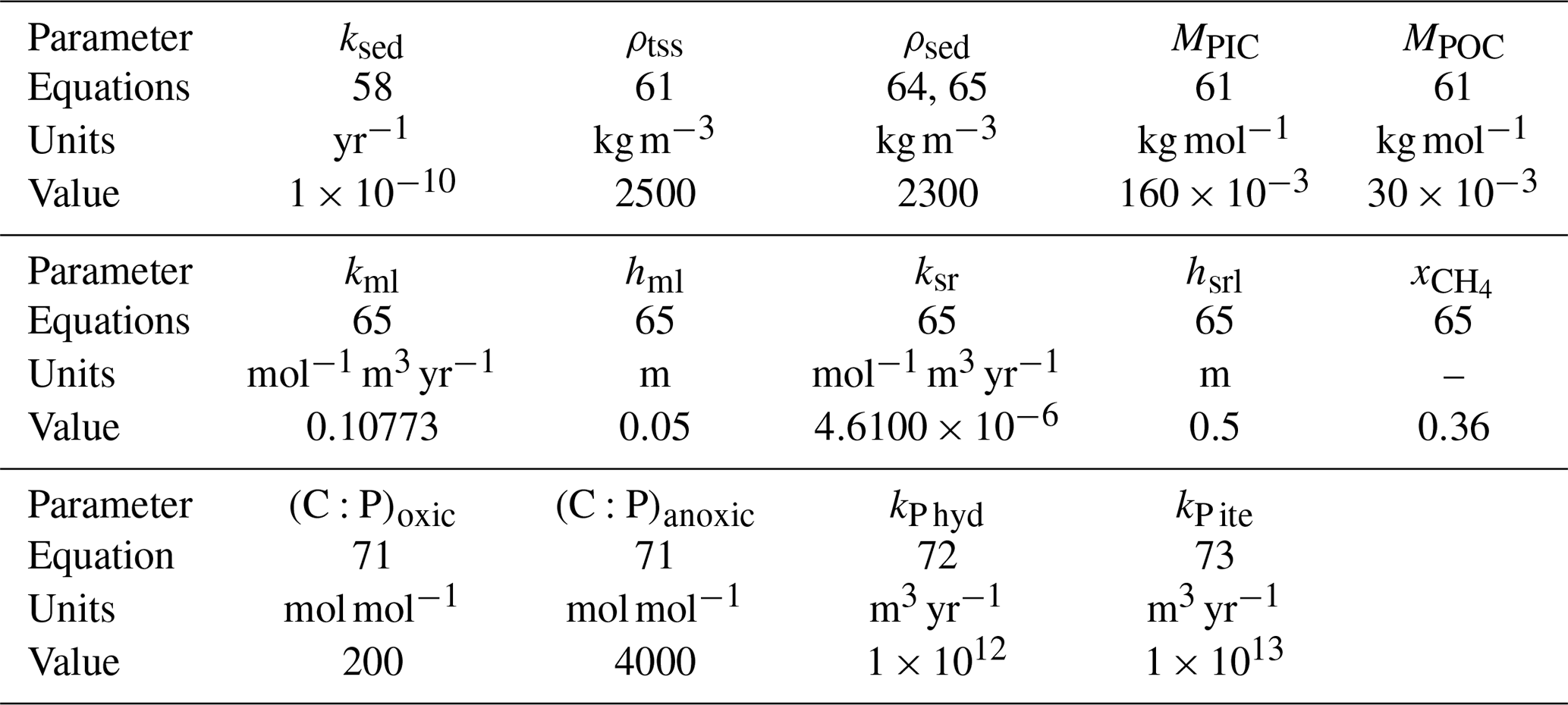
The early diagenesis module uses the same discretization (boxes) as the oceanic module, but only the boxes intercepting the seafloor ($A_i^{\text{sf}}>\mathrm{0}$) are considered. For instance, in the default GEOCLIM configuration (see Sect. 2.2.1), the early diagenesis module includes all the oceanic boxes except #3, “midlatitude surface”. The values of all parameters of the early diagenesis module's equations are listed in Table 3.

Table 3 Early diagenesis module parameters.

We use the following naming convention concerning the fluxes within the early diagenesis module: “raining” fluxes (F_rain) are fluxes of settling particles that have just reached the seafloor (while “sinking” fluxes refer to the settling particles that are still in the water column). “Deposition” fluxes (F_dep) are fluxes of sediments on the seafloor after their downslope lateral transfer between adjacent GEOCLIM boxes that will stay in the current box. “Burial” fluxes (F_bur) are fluxes of deposited elements that have undergone all the chemical reactions of early diagenesis. Burial fluxes are the actual sinks of chemical elements from the ocean–atmosphere reservoir.

2.3.1 Raining fluxes towards the ocean floor and sediments

The raining fluxes are computed for the four particulate variables: particulate inorganic carbon (PIC), particulate organic carbon (POC), particulate organic phosphorus (POP), and strontium associated with PIC (Sr_PIC). For each box i, the raining flux of a particulate variable Y is

$$\begin{array}{}\text{(57)}& F_{\text{rain}}(\mathrm{Y}{)}_{\left(i\right)}=w_{\text{sink}}{A}_i^{\text{sf}}[\mathrm{Y}{]}_i.\end{array}$$

This equation can be directly deduced from the net sinking flux on each box (Eq. 44). Raining fluxes are the fluxes of material “lost” from the oceanic module and transferred to the early diagenesis module.

2.3.2 Lateral advection fluxes and deposition fluxes

Particles sedimenting on the seafloor are subject to lateral advection from upslope GEOCLIM boxes to downslope boxes. This advection is meant to represent turbidity currents. The approach adopted to compute those advection fluxes is to define, for each box, a sediment accumulation capacity and to export downslope whatever exceeds this capacity. This scheme was introduced in Maffre et al. (2021) but was revisited in the current study, firstly to represent the export of POC and POP (Eq. 63), while Maffre et al. (2021) only considered the export of bulk sediment, and secondly to introduce a new method to determine the box-to-box sediment routing (Eq. 62).

First, the ocean seafloor is vertically discretized into four levels, from shallower to deeper: coastal surface, coastal non-surface, open-ocean intermediate depth, and open-ocean deep. They correspond to the definition of GEOCLIM boxes based on seafloor depth (traditionally, 0–100 m, 100–200 m, 200–1000 m, and >1000 m; see Sect. 2.2.1). In other words, the boxes in the level “coastal surface” are all the boxes where the seafloor depth is 0–100 m and similarly for all vertical levels. In the default GEOCLIM configuration (see Sect. 2.2.1), the definition of the vertical levels is as follows.

1. Coastal surface: box #6

2. Coastal non surface: box #7

3. Open-ocean intermediate depth: boxes # 1, 4, and 8

4. Open-ocean deep: boxes # 2, 5, and 9

The sediment accumulation capacity C is first determined for the four vertical levels, with ℒ being a given vertical level:

$$\begin{array}{ll}{\displaystyle }{A}_{\mathcal{L}}^{\text{sf}}=& {\displaystyle }\sum _{i\in \mathit{\left\{}\mathcal{L}\mathit{\right\}}}{A}_i^{\text{sf}}\\ \text{(58)}& {\displaystyle }{C}_{\mathcal{L}}=& {\displaystyle }{k}_{\text{sed}}(A_{\mathcal{L}}^{\text{sf}}{)}^{\mathrm{3}/\mathrm{2}}.\end{array}$$

The seafloor area of a vertical level ℒ is simply the sum of seafloor areas of all boxes within that level. The scaling with an exponent $\mathrm{3}/\mathrm{2}$ represents the approximation of wedge geometry, where the volume of a wedge is proportional to its basal area at the power $\mathrm{3}/\mathrm{2}$. The sediment accumulation capacity of a given box i that is in the vertical level ℒ(i) is calculated on a pro rata basis:

$$\begin{array}{}\text{(59)}& C_i={\displaystyle \frac{A_i^{\text{sf}}}{A_{\mathcal{L}\left(i\right)}^{\text{sf}}}}{C}_{\mathcal{L}\left(i\right)}.\end{array}$$

The accumulation capacity is then used to determine, for each box i and at each time step, the proportion of material that stays in place $x_i^{\text{dep}}$ (the fraction that is exported downslope being $\mathrm{1}-x_i^{\text{dep}}$):

$$\begin{array}{ll}{\displaystyle }& {\displaystyle }{x}_i^{\text{dep}}={\displaystyle \frac{\mathrm{1}}{\mathrm{1}+F_{\text{sed}}^{\text{in}}(\text{bulk}{)}_{\left(i\right)}/\left({\mathit{\rho }}_{\text{sed}}{C}_i\right)}}\\ \text{(60)}& {\displaystyle }& {\displaystyle }{F}_{\text{dep}}(\text{bulk}{)}_{\left(i\right)}=x_i^{\text{dep}}{F}_{\text{sed}}^{\text{in}}(\text{bulk}{)}_{\left(i\right)},\end{array}$$

where ρ_sed is the density of marine sediment (set to 2300 kg m⁻³), $F_{\text{sed}}^{\text{in}}(\text{bulk}{)}_{\left(i\right)}$ is the total incoming bulk sediment flux in the box i (i.e., the sum of all particles' raining fluxes, sediment exported from upslope or from continental inputs), and F_dep(bulk)_(i) is the “net” deposition flux of sediment in the box i. A Michaelis-like saturating function is used in Eq. (60) to ensure a smooth transition and avoid an abrupt threshold when the sedimentation flux reaches the accumulation capacity.

$F_{\text{sed}}^{\text{in}}(\text{bulk}{)}_{\left(i\right)}$ is calculated as follows.

$$\begin{array}{}\text{(61)}& \begin{array}{rl}{F}_{\text{sed}}^{\text{in}}(\text{bulk}{)}_{\left(i\right)}=& M_{\text{PIC}}{F}_{\text{rain}}(\text{PIC}{)}_{\left(i\right)}\\ & +M_{\text{POC}}{F}_{\text{rain}}(\text{POC}{)}_{\left(i\right)}+{\mathit{\rho }}_{\text{tss}}{E}_{\left(i\right)}\\ & +\sum _j{F}_{\text{sed}}^{\text{adv}}(\text{bulk}{)}_{ji}\end{array}\end{array}$$

Here, M_PIC and M_POC are the molecular weight of PIC and POC (respectively), ρ_tss is the density of continental sediments set to 2500 kg m⁻³, E_(i) is the erosion flux integrated for the continental drainage basin of box i, and $F_{\text{sed}}^{\text{adv}}(\text{bulk}{)}_{ji}$ is the flux of bulk sediment laterally advected on the seafloor from box j to box i.

$F_{\text{sed}}^{\text{adv}}(\text{bulk}{)}_{ji}$ is determined using the “cross-level boundary length matrix” L: L_ji is the length of the boundary between box j and box i if box j is in a vertical level immediately above box i. For instance, L_ji is 0 if j and i are two coastal surface boxes, even if they are adjacent. L_ji is also 0 if j and i are, for instance, a coastal surface box and an open-ocean intermediate box (because the “coastal non-surface” level is between them). Lastly, if L_ji is >0, then L_ij must be 0 (because i is in the vertical level below j). $F_{\text{sed}}^{\text{adv}}(\text{bulk}{)}_{ji}$ is then calculated on a pro rata basis of the length of the “cross-level” boundaries of box j:

$$\begin{array}{}\text{(62)}& F_{\text{sed}}^{\text{adv}}(\text{bulk}{)}_{ji}={\displaystyle \frac{L_{ji}}{{\sum }_k{L}_{jk}}}(\mathrm{1}-x_j^{\text{dep}}\left)F_{\text{sed}}^{\text{in}}\right(\text{bulk}{)}_{\left(j\right)}.\end{array}$$

This pro rata distribution of downslope (cross-level) exported sediment fluxes is illustrated in Fig. 2. One may note an apparent circularity in Eqs. (60)–(62), where x^dep depends on $F_{\text{sed}}^{\text{in}}$ that depends on $F_{\text{sed}}^{\text{adv}}$, itself depending on x^dep. These equations can actually be solved straightforwardly from upslope to downslope. $F_{\text{sed}}^{\text{in}}$ is first calculated for all coastal surface boxes, where the term $F_{\text{sed}}^{\text{adv}}$ is null (no upslope boxes), and x^dep is deduced from $F_{\text{sed}}^{\text{in}}$. Then, $F_{\text{sed}}^{\text{in}}$ is calculated for all coastal non-surface boxes, where $F_{\text{sed}}^{\text{adv}}$ terms come from coastal surface boxes, whose x^dep values were just calculated, and so on until the open-ocean deep boxes.

Finally, the deposition fluxes of POC and POP (F_dep(Y)_(i), where Y is either POC or POP) are computed on a similar basis (and also from upslope to downslope).

$$\begin{array}{ll}{\displaystyle }{F}_{\text{sed}}^{\text{in}}(\mathrm{Y}{)}_{\left(i\right)}& {\displaystyle }=F_{\text{rain}}(\mathrm{Y}{)}_{\left(i\right)}+\sum _j{F}_{\text{sed}}^{\text{adv}}(\mathrm{Y}{)}_{ji}\\ {\displaystyle }{F}_{\text{sed}}^{\text{adv}}(\mathrm{Y}{)}_{ji}& {\displaystyle }={\displaystyle \frac{L_{ji}}{{\sum }_k{L}_{jk}}}(\mathrm{1}-x_j^{\text{dep}})F_{\text{sed}}^{\text{in}}(\mathrm{Y}{)}_{\left(j\right)}\\ \text{(63)}& {\displaystyle }{F}_{\text{dep}}(\mathrm{Y}{)}_{\left(i\right)}& {\displaystyle }=x_i^{\text{dep}}{F}_{\text{sed}}^{\text{in}}(\mathrm{Y}{)}_{\left(i\right)}\end{array}$$

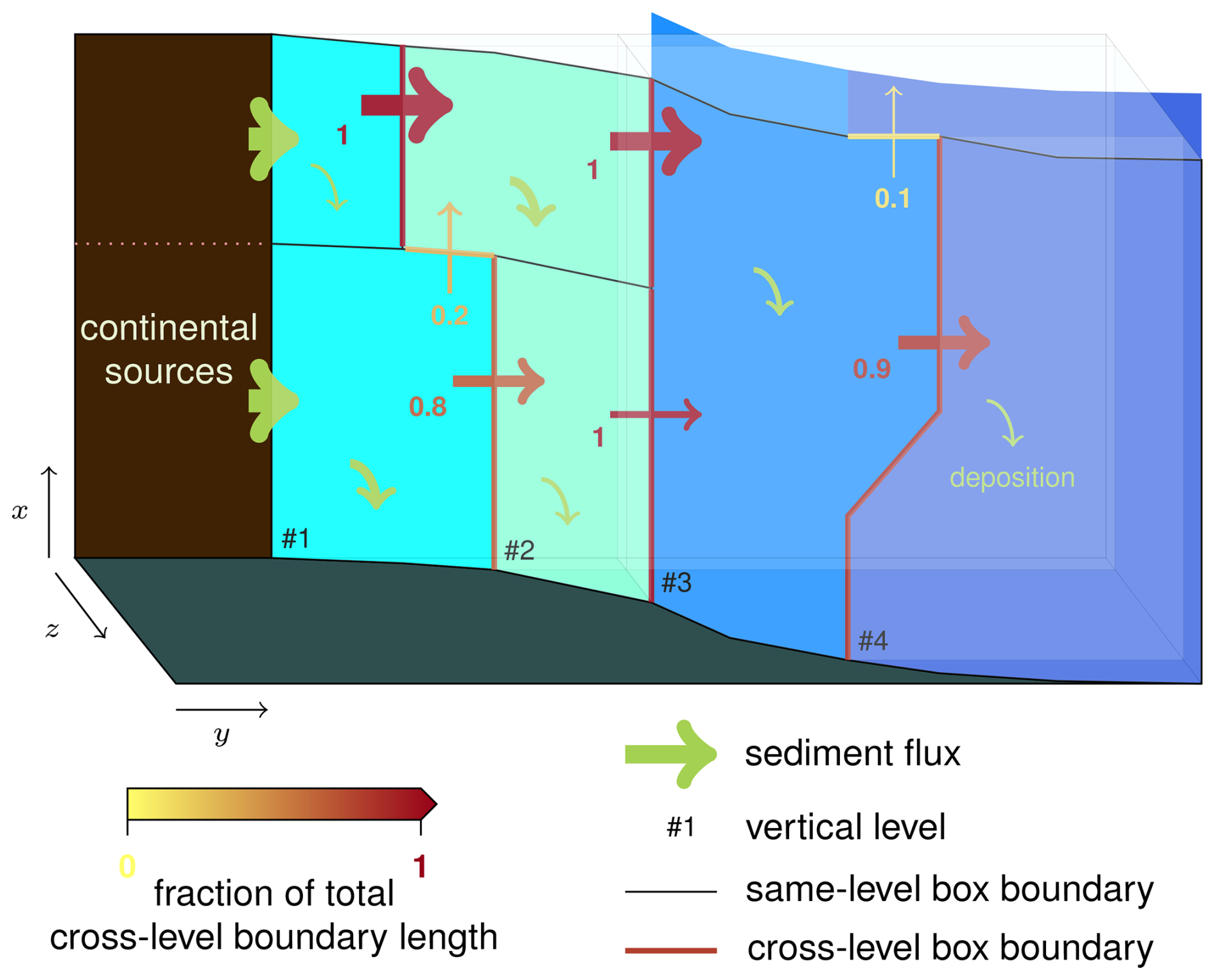
Figure 2 Schematics of the seafloor sediment routing scheme, illustrating the four vertical levels on the seafloor. All sediments that are not deposited in a current box are exported to the next-level boxes and distributed proportionally to the fraction of the total length of cross-level (downslope) boundaries of the current box (cf. Eq. 62). The arrow width (both transport and deposition) is meant to represent the absolute sediment fluxes, while the colors and numbers represent the fraction of the downward (cross-level) fluxes.

F_dep(PIC)_(i) is not computed because all PIC raining on the seafloor is eventually buried (no re-dissolution in sediments), and the contribution to bulk sediment fluxes is already taken into account (Eq. 61). Hence, it is not necessary to track PIC on the seafloor by computing the advection and deposition fluxes.

The introduction of the cross-level boundary length matrix L is an innovation of the present study. For retro-compatibility with the version of GEOCLIM published in Maffre et al. (2021), an option is left to compute $F_{\text{sed}}^{\text{adv}}$ without the matrix L, considering that sediments of a given box i are exported on all the boxes of the vertical level immediately below i (not just the adjacent ones) on a pro rata basis of their seafloor area.

2.3.3 Early diagenesis chemical reactions and burial fluxes

The computation of the chemical reactions associated with early diagenesis was not changed from Maffre et al. (2021). Early diagenesis is simulated, for each box, by a vertical reactive transport model within two successive layers: a bioturbated (mixed) sediment layer, where organic carbon can be oxidized by dissolved O₂, followed by a layer where organic carbon can be oxidized by ${\mathrm{SO}}_{\mathrm{4}}^{\mathrm{2}-}$ (i.e., sulfate reduction layer). The last considered reaction, methanogenesis (i.e., dismutation of organic carbon in CH₄ and CO₂), is not computed by an advection–reaction framework. No other chemical reaction is considered in the GEOCLIM early diagenesis module. Moreover, the fluxes are computed assuming that the reactive transport is at steady state.

The “advection” part is caused by sediment accumulation, which is equivalent to downward vertical advection of material, with respect to the seafloor. The sedimentation rate $w_i^{\mathrm{s}}$ in a given box i is defined as

$$\begin{array}{}\text{(64)}& w_i^{\mathrm{s}}={\displaystyle \frac{F_{\text{dep}}(\text{bulk}{)}_{\left(i\right)}}{{\mathit{\rho }}_{\text{sed}}.A_i^{\text{sf}}}}.\end{array}$$

While traveling through the two layers, organic carbon is oxidized, either by O₂ or ${\mathrm{SO}}_{\mathrm{4}}^{\mathrm{2}-}$, and the oxidation rate per unit of volume is proportional to $\stackrel{\mathrm{‾}}{\left[\mathrm{C}\right]}\left[\text{oxidant}\right]$. The oxidant concentration is the oceanic one (in the local oceanic box), and $\stackrel{\mathrm{‾}}{\left[\mathrm{C}\right]}$ is the average organic carbon concentration in the layer. With [C]^o, [C]^ml, and [C]^srl being the concentrations of organic C at the top of sediment, in the mixed layer, and in the sulfate reduction layer (respectively) and h_ml and h_sr being the thicknesses of the mixed and sulfate reduction layers (respectively), we have the following.

$$\begin{array}{ll}{\displaystyle }[\mathrm{C}{]}_i^{\mathrm{o}}& {\displaystyle }={\displaystyle \frac{F_{\text{dep}}(\text{POC}{)}_{\left(i\right)}}{F_{\text{dep}}(\text{bulk}{)}_{\left(i\right)}/{\mathit{\rho }}_{\text{sed}}}}\\ {\displaystyle }[\mathrm{C}{]}_i^{\text{ml}}& {\displaystyle }={\displaystyle \frac{w_i^{\mathrm{s}}[\mathrm{C}{]}_i^{\mathrm{o}}}{w_i^{\mathrm{s}}+k_{\text{ml}}\left[{\mathrm{O}}_{\mathrm{2}}\right]h_{\text{ml}}}}\\ \text{(65)}& {\displaystyle }[\mathrm{C}{]}_i^{\text{srl}}& {\displaystyle }={\displaystyle \frac{w_i^{\mathrm{s}}[\mathrm{C}{]}_i^{\text{ml}}}{w_i^{\mathrm{s}}+k_{\text{sr}}\left[{\mathrm{SO}}_{\mathrm{4}}^{\mathrm{2}-}\right]h_{\text{srl}}}}\end{array}$$

Here, k_ml and k_sr are kinetics constants. We use a different notation for the concentration of organic C in the sediment to avoid confusion with [POC], which is the concentration of organic carbon in seawater.

Methanogenesis is assumed to consume a fixed fraction $x_{{\mathrm{CH}}_{\mathrm{4}}}$ of the organic C remaining after sulfate reduction. The produced methane is further assumed to leak back to the ocean and be oxidized by O₂. Thus, the organic carbon burial flux in the box i is

$$\begin{array}{}\text{(66)}& F_{\text{bur}}(\mathrm{POC}{)}_{\left(i\right)}=(\mathrm{1}-x_{{\mathrm{CH}}_{\mathrm{4}}}\left)w_i^{\mathrm{s}}{A}_i^{\text{sf}}\right[\mathrm{C}{]}_i^{\text{srl}}.\end{array}$$

And the CO₂ flux from sediment to the ocean in the box i (${F_{\text{sed}}^{{\mathrm{CO}}_{\mathrm{2}}}}_{\left(i\right)}$, used in Eq. 1) is

$$\begin{array}{}\text{(67)}& {F_{\text{sed}}^{{\mathrm{CO}}_{\mathrm{2}}}}_{\left(i\right)}=F_{\text{dep}}(\text{POC}{)}_{\left(i\right)}-F_{\text{bur}}(\mathrm{POC}{)}_{\left(i\right)}.\end{array}$$

The sulfate reduction flux (i.e., the flux of ${\mathrm{SO}}_{\mathrm{4}}^{\mathrm{2}-}$ consumed by sulfate reduction, ${F_{\text{SR}}}_{\left(i\right)}$, used in Eqs. 3 and 8) is

$$\begin{array}{}\text{(68)}& {F_{\text{SR}}}_{\left(i\right)}={\displaystyle \frac{\mathrm{1}}{\mathrm{2}}}{w}_i^{\mathrm{s}}{A}_i^{\text{sf}}\left(\right[\mathrm{C}{]}_i^{\text{ml}}-\left[\mathrm{C}{]}_i^{\text{srl}}\right).\end{array}$$

The coefficient $\frac{\mathrm{1}}{\mathrm{2}}$ arises from the stoichiometry of the sulfate reduction reaction (two moles of C oxidized for one mole of S reduced).

The total consumption of oxygen by all early diagenesis processes ($F_{\text{sed}}^{{\mathrm{O}}_{\mathrm{2}}}$, used in Eq. 6) is as follows.

$$\begin{array}{}\text{(69)}& \begin{array}{rl}{F}_{{\text{sed}}_{\left(i\right)}}^{{\mathrm{O}}_{\mathrm{2}}}=w_i^{\mathrm{s}}{A}_i^{\text{sf}}(& \left(\right[\mathrm{C}{]}_i^{\mathrm{o}}-\left[\mathrm{C}{]}_i^{\text{ml}}\right)\\ & +{\displaystyle \frac{\mathrm{1}}{\mathrm{8}}}\left(\right[\mathrm{C}{]}_i^{\text{ml}}-\left[\mathrm{C}{]}_i^{\text{srl}}\right)+x_{{\mathrm{CH}}_{\mathrm{4}}}\left[\mathrm{C}{]}_i^{\text{srl}}\right)\end{array}\end{array}$$

This equation accounts for (1) the sulfate reduction stoichiometry, where for one reduced S unit, $\mathrm{1}/\mathrm{2}$ Fe²⁺ is released (and hence $\mathrm{1}/\mathrm{8}$ O₂ is eventually consumed to oxidize it in Fe³⁺), and (2) the assumption that all leaking methane is oxidized by O₂.

2.3.4 Phosphorus fluxes in early diagenesis

Phosphorus differs from the other elements in that sediments can act both as a source and a sink of H₃PO₄ because of additional processes that capture dissolved phosphate. The computation of these processes was not changed from Maffre et al. (2021).

The burial flux of phosphorus associated with organic carbon F_bur(POP) is scaled to the organic carbon burial flux F_bur(POC), but with a C:P ratio specific to local conditions.

$$\begin{array}{}\text{(70)}& F_{\text{bur}}\left(\text{POP}\right)={\displaystyle \frac{F_{\text{bur}}\left(\mathrm{POC}\right)}{(\mathrm{C}:\mathrm{P}{)}_{\text{burial}}}}\end{array}$$

That ratio (C:P)_burial is parameterized with the degree of anoxia (DOA).

$$\begin{array}{}\text{(71)}& \begin{array}{rl}\left(\mathrm{C}:\mathrm{P}\right)& {}_{\text{burial}}=\\ & {\displaystyle \frac{(\mathrm{C}:\mathrm{P}{)}_{\text{oxic}}\cdot (\mathrm{C}:\mathrm{P}{)}_{\text{anoxic}}}{(\mathrm{1}-\text{DOA})\cdot (\mathrm{C}:\mathrm{P}{)}_{\text{anoxic}}+\text{DOA}\cdot (\mathrm{C}:\mathrm{P}{)}_{\text{oxic}}}}\end{array}\end{array}$$

In other words, the amount of P buried for a given amount of buried C varies linearly with the DOA between the two end-members. The DOA qualitatively represents the fraction of the box that is anoxic. It varies from 1 (fully anoxic basin) to 0 (fully oxic basin). It is made depending on the local oceanic O₂ concentration with a polynomial fit of relation of Van Cappellen and Ingall (1994, Fig. 4a of their contribution). See also Maffre et al. (2021) (Fig. S1 of their contribution). Roughly speaking, it linearly decreases from 1 for [${\mathrm{O}}_{\mathrm{2}}]=\mathrm{0}\mathrm{mol}{\mathrm{m}}^{-\mathrm{3}}$ to 0 for $\left[{\mathrm{O}}_{\mathrm{2}}\right]=\mathrm{0.4}\mathrm{mol}{\mathrm{m}}^{-\mathrm{3}}$. The end-member burial C:P ratios are $(\mathrm{C}:\mathrm{P}{)}_{\text{oxic}}=\mathrm{200}$ and $(\mathrm{C}:\mathrm{P}{)}_{\text{anoxic}}=\mathrm{4000}$.

Two additional sinks of phosphorus are considered: hydrothermal burial F_P hyd and burial in the form of phosphorite F_P ite; both of them are proportional to the dissolved phosphorus concentration and are computed only in open-ocean deep boxes.

$$\begin{array}{}\text{(72)}& {\displaystyle }& {\displaystyle }{F_{\mathrm{P}\text{hyd}}}_{\left(i\right)}=k_{\mathrm{P}\text{hyd}}[{\mathrm{H}}_{\mathrm{3}}{\mathrm{PO}}_{\mathrm{4}}{]}_i\text{(73)}& {\displaystyle }& {\displaystyle }{F_{\mathrm{P}\text{ite}}}_{\left(i\right)}=k_{\mathrm{P}\text{ite}}[{\mathrm{H}}_{\mathrm{3}}{\mathrm{PO}}_{\mathrm{4}}{]}_i\end{array}$$

Therefore, the net flux of phosphorus from sediment to ocean in the box i ($F_{\mathrm{P}\text{sed}}^{\text{net}}$, used in Eq. 4) is

$$\begin{array}{}\text{(74)}& \begin{array}{rl}{F_{\mathrm{P}\text{sed}}^{\text{net}}}_{\left(i\right)}=& F_{\text{dep}}(\text{POP}{)}_{\left(i\right)}-F_{\text{bur}}(\mathrm{POP}{)}_{\left(i\right)}\\ & -{F_{\mathrm{P}\text{hyd}}}_{\left(i\right)}-{F_{\mathrm{P}\text{ite}}}_{\left(i\right)}.\end{array}\end{array}$$

2.4 Continental weathering

The current version of the continental module of GEOCLIM has been developed and introduced in Maffre et al. (2021), with the exception of carbonate weathering that has not changed since Arndt et al. (2011). This module is designed to have the same geographic grid as the GCM coupled to GEOCLIM, with a typical resolution of a few degrees in longitude and latitude, but it does not need to be a rectilinear longitude–latitude grid. It is still possible to use a different grid, for instance one at higher resolution, by interpolating all the climate fields needed by the continental module (see Sect. 3.1) on that new grid. This module calculates the seven following spatially resolved fluxes over the continental surface:

• physical erosion ($\stackrel{,,}{E}$, in m yr⁻¹),

• silicate weathering (${\stackrel{,,}{F}}_{\text{silw}}$, in $\mathrm{mol}{\mathrm{m}}^{-\mathrm{2}}{\mathrm{yr}}^{-\mathrm{1}}$),

• carbonate weathering (${\stackrel{,,}{F}}_{\text{carw}}$, in $\mathrm{mol}{\mathrm{m}}^{-\mathrm{2}}{\mathrm{yr}}^{-\mathrm{1}}$),

• petrogenic organic C weathering (${\stackrel{,,}{F}}_{\text{focw}}$, in $\mathrm{mol}{\mathrm{m}}^{-\mathrm{2}}{\mathrm{yr}}^{-\mathrm{1}}$),

• sulfide weathering (${\stackrel{,,}{F}}_{\text{sulw}}$, in $\mathrm{mol}{\mathrm{m}}^{-\mathrm{2}}{\mathrm{yr}}^{-\mathrm{1}}$),

• biospheric organic C export (${\stackrel{,,}{F}}_{\text{bocx}}$, in $\mathrm{mol}{\mathrm{m}}^{-\mathrm{2}}{\mathrm{yr}}^{-\mathrm{1}}$), and

• phosphorus weathering (${\stackrel{,,}{F}}_{\text{phow}}$, in $\mathrm{mol}{\mathrm{m}}^{-\mathrm{2}}{\mathrm{yr}}^{-\mathrm{1}}$).

In the entire article, we use the writing convention $\stackrel{,,}{F}$ to indicate a specific continental flux (in $\mathrm{mol}{\mathrm{m}}^{-\mathrm{2}}{\mathrm{yr}}^{-\mathrm{1}}$), while F would be the corresponding intensive flux (in mol yr⁻¹). All the continental fluxes are computed as a function of the following variables:

• T, the surface temperature, at the current CO₂ level (in K)

• q, the total runoff, i.e, precipitation minus evaporation, at the current CO₂ level (in m yr⁻¹)

• S, the topographic slope (in m m⁻¹)

• x_L(l), the area fraction of a grid cell covered by the lithological class l

The required temperature and runoff fields are generated by the GCM simulations and are annual mean climatological averages (e.g., average over 30 years of equilibrium climate). The slope field is the gradient of high-resolution elevation (i.e., ridge crests and ravines). At the present day (for calibration purposes or for pre-industrial simulations), we used the Shuttle Radar Topography Mission (SRTM) digital elevation model at 30^′′ resolution and then averaged at the nominal continental resolution of GEOCLIM. In the past, the slope was calculated from a guess of the continental elevations based on geological and/or paleontological data taken from the literature, but in GEOCLIM7, a new method is added (see Sect. 3.4.1). The lithological classes can be user-defined. The standard lithology definition of the model is as follows:

1. metamorphic

2. mafic and ultramafic

3. intermediate

4. felsic

5. siliciclastic sediments

6. carbonate

For deep time, the lithology is generally poorly constrained. GEOCLIM is then often run with a simplified lithology, limited to three classes: granites, basalts, and carbonates.

2.4.1 Erosion

The physical erosion rate is calculated for each continental grid cell. The equation is derived from the stream power incision model (e.g., Davy and Crave, 2000) and adapted for a regular longitude–latitude grid as in Maffre et al. (2018):

$$\begin{array}{}\text{(75)}& \stackrel{,,}{E}=k_{\mathrm{e}}{q}^{\mathrm{0.5}}S,\end{array}$$

where k_e is the erodibility constant.

2.4.2 Silicate weathering: DynSoil model

Compared to other deep-time models, a unique feature of the GEOCLIM model is its ability to simulate the coupling between physical erosion and chemical alteration of continental surfaces.

The silicate weathering model of GEOCLIM has been derived from the Gabet and Mudd (2009) regolith model (with the parameterization of West, 2012) to represent its transient evolution. This model is called DynSoil and was first published in Maffre et al. (2022), while Park et al. (2020) published the steady-state version of this model, coupled to an inverse model for equilibrium pCO₂.

We consider the “regolith” to be the interface between unweathered bedrock and the Earth's surface, where the chemical weathering reactions occur. The general operation of DynSoil is based on a change of reference frame. The regolith does not descend into the parent rock, but it is the parent rock that sends blocks of rock into the regolith. The DynSoil weathering model is based on two assumptions. Firstly, the transformation of parent rock into regolith does not consume CO₂ because this initial phase of alteration is essentially driven by redox reactions (Buss et al., 2008; Brantley and White, 2009). The second hypothesis is that the regolith is where CO₂ is consumed by chemical alteration. As the blocks rise to the surface, they are gradually altered chemically, consuming atmospheric CO₂ and gradually reducing their abundance. When they reach the surface, the surviving particles are swept away by physical erosion.

The regolith model dynamically calculates the abundance of primary minerals all along the regolithic profile and for each continental grid cell. In addition to temperature and runoff, the DynSoil model accounts for a third key variable in weathering calculation: the regolith thickness h. h is calculated at each time step and for each continental grid cell as follows.

$$\begin{array}{}\text{(76)}& {\displaystyle \frac{\mathrm{d}h}{\mathrm{d}t}}=P_{\mathrm{o}}f\left(h\right)-\stackrel{,,}{E}\end{array}$$

P_o is the optimal regolith production rate, computed as

$$\begin{array}{}\text{(77)}& P_{\mathrm{o}}=k_{\text{rp}}q{e}^{-\frac{{E_{\mathrm{A}}}_{\text{rp}}}{R}(\frac{\mathrm{1}}{T}-\frac{\mathrm{1}}{T_{\mathrm{o}}})},\end{array}$$

where R is the ideal gas constant, T_o the chosen reference temperature (288.15 K), ${E_{\mathrm{A}}}_{\text{rp}}$ the apparent activation energy at T_o for regolith production, and k_rp the proportionality constant.

f(h) is the soil production function. This function simulates the decrease in the regolith production rate with the thickness of the regolith. The hypothesis behind the introduction of a soil production function is the decrease in the water percolation when the regolith thickness rises, limiting the regolith production at the interface between the regolith and the bedrock. According to Heimsath et al. (1997), we implement an exponential soil production function:

$$\begin{array}{}\text{(78)}& f\left(h\right)=e^{-h/h_{\mathrm{o}}},\end{array}$$

where h_o is the decay depth.

The vertical profile of primary minerals x_p follows an advection–reaction equation (the downward migration of regolith–bedrock transition is equivalent to an upward advection of rock particles).

$$\begin{array}{ll}{\displaystyle \frac{\partial x_{\mathrm{p}}}{\partial t}}+P_{\mathrm{o}}f\left(h\right){\displaystyle \frac{\partial x_{\mathrm{p}}}{\partial z}}& {\displaystyle }=-K{\mathit{\tau }}^{\mathit{\sigma }}{x}_{\mathrm{p}}\\ \text{(79)}& {\displaystyle \frac{\partial \mathit{\tau }}{\partial t}}+P_{\mathrm{o}}f\left(h\right){\displaystyle \frac{\partial \mathit{\tau }}{\partial z}}& {\displaystyle }=\mathrm{1}\end{array}$$

The vertical coordinate z varies from 0 at the regolith–bedrock interface to h at the surface (i.e., z is positive upward). τ is the “age” of rock particles at the local depth that is the time elapsed since the particle has entered the regolith. Kτ^σ can be seen as the dissolution rate constant of a first-order reaction. The exponent σ simulates the decrease in the rate constant with the age of the particle (as σ<0). K is defined according to the following equation:

$$\begin{array}{}\text{(80)}& K=k_{\mathrm{d}}(\mathrm{1}-e^{-k_{\mathrm{w}}q})e^{-\frac{{E_{\mathrm{A}}}_{\mathrm{d}}}{R}(\frac{\mathrm{1}}{T}-\frac{\mathrm{1}}{T_{\mathrm{o}}})},\end{array}$$

where k_w is the runoff saturation parameter, ${E_{\mathrm{A}}}_{\mathrm{d}}$ the apparent activation energy at the reference temperature T_o for mineral dissolution, and k_d the dissolution constant (West, 2012).

Finally, the silicate weathering rate is calculated as the dissolution rate integrated over the regolith from the bedrock interface (h=0) to the top of the regolith:

$$\begin{array}{}\text{(81)}& {\stackrel{,,}{F}}_{\text{silw}}\left(l\right)={\mathit{\chi }}_{\mathrm{CaMg}}\left(l\right)\underset{\mathrm{0}}{\overset{\mathrm{h}}{\int }}K{\mathit{\tau }}^{\mathit{\sigma }}{x}_{\mathrm{P}}\mathrm{d}z,\end{array}$$

where χ_CaMg is the amount of calcium and magnesium per m³ of bedrock (x_P is the fraction of primary minerals in the regolith normalized to the one of the bedrock). Only calcium and magnesium are accounted for in the weathering flux calculation, as they are the only cations involved in carbonate sedimentation (see also Sect. 2.2.10). The silicate weathering rate is then expressed in $\mathrm{mol}\mathrm{CaMg}{\mathrm{m}}^{-\mathrm{2}}{\mathrm{yr}}^{-\mathrm{1}}$.

The index (l) in Eq. (81) indicates that silicate weathering is computed for each silicate lithological class (five are traditionally considered). All the parameters described in the current section (2.4.2) are actually lithology-dependent (see Table 4), although the indexation (l) was omitted in previous equations for the sake of readability. If N_sil is the number of silicate lithological class, the total silicate weathering rate is then

$$\begin{array}{}\text{(82)}& {\stackrel{,,}{F}}_{\text{silw}}=\sum _{l=\mathrm{1}}^{N_{\text{sil}}}{x}_L\left(l\right){\stackrel{,,}{F}}_{\text{silw}}\left(l\right).\end{array}$$

Table 4 Continental parameters. The abbreviated lithologies are metamorphic (metam.), intermediate (interm.), siliclastic sediments (sil. sed.), and carbonate (carb.). Where one value is given, it applies to all lithologies.

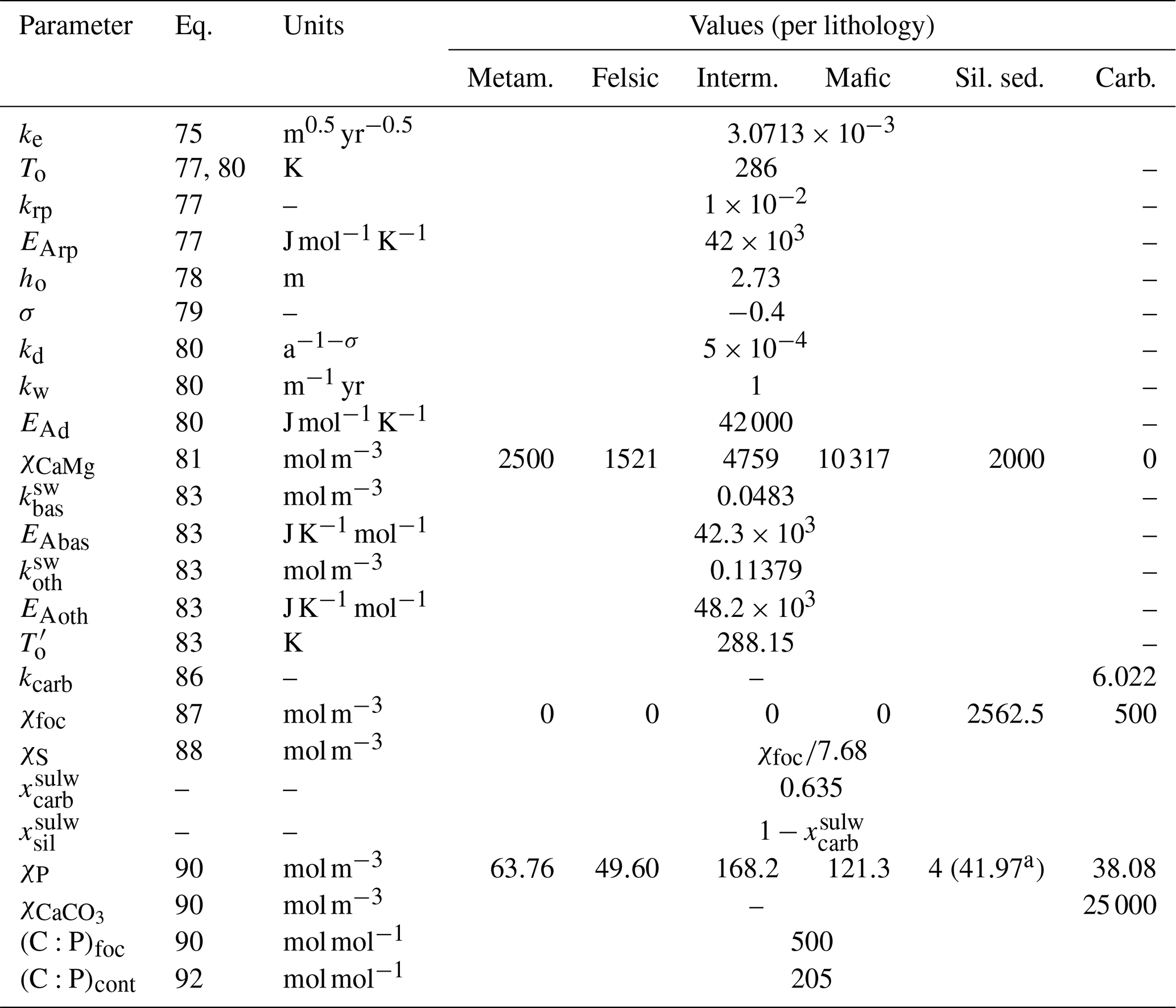
^a The Hartmann et al. (2014) value.

2.4.3 Alternative silicate weathering model

For retro-compatibility, an option is left in GEOCLIM for computing silicate weathering fluxes without the DynSoil model using empirical relationships (Dessert et al., 2003; Oliva et al., 2003).

$$\begin{array}{l}{\displaystyle }{\stackrel{,,}{F}}_{\text{silw}}\left(l_{\text{bas}}\right)=k_{\text{bas}}^{\text{sw}}q{e}^{-\frac{{E_{\mathrm{A}}}_{\text{bas}}}{R}(\frac{\mathrm{1}}{T}-\frac{\mathrm{1}}{T_{\mathrm{o}}^{\prime }})}\\ \text{(83)}& {\displaystyle }{\stackrel{,,}{F}}_{\text{silw}}\left(l_{\text{oth}}\right)=k_{\text{oth}}^{\text{sw}}q{e}^{-\frac{{E_{\mathrm{A}}}_{\text{oth}}}{R}(\frac{\mathrm{1}}{T}-\frac{\mathrm{1}}{T_{\mathrm{o}}^{\prime }})}\end{array}$$

Here, l_bas is the lithological class corresponding to basalts, and l_oth is the lithological class corresponding to all the other silicates.

2.4.4 Carbonate weathering

Given the fast dissolution rate of carbonate minerals, we assume that carbonate weathering operates in a thermodynamically limited regime, whatever the location on the continents (Arndt et al., 2011). We first calculate the dissolved calcium concentration in the water percolating through soils assuming that the soil water is at equilibrium with pure calcite at the local belowground CO₂ level pCO₂|_soil. Due to the root respiration and the decay of organic matter, the ambient soil CO₂ increases down to the root zone. Below the roots, the CO₂ level stays constant at its maximum value. The maximum pCO₂ (PAL) in soil is defined as follows (Lieth, 1984):

$$\begin{array}{}\text{(84)}& p{\mathrm{CO}}_{\mathrm{2}}{|}_{\text{soil}}^{\text{max}}=\mathrm{1}+\mathrm{0.302484}{q}^{\mathrm{0.8}},\end{array}$$

where q, the local runoff, is expressed here in cm yr⁻¹. Then, the actual pCO₂|_soil is computed by weighting the maximum soil CO₂ by a factor depending on the local temperature. Indeed, when temperature rises, the decay of organic matter is accelerated, according to (Gwiazda and Broecker, 1994)

$$\begin{array}{}\text{(85)}& p{\mathrm{CO}}_{\mathrm{2}}{|}_{\text{soil}}=p{{\mathrm{CO}}_{\mathrm{2}}}^{\text{atm}}+{\displaystyle \frac{p{\mathrm{CO}}_{\mathrm{2}}{|}_{\text{soil}}^{\text{max}}}{\mathrm{1}+e^{\left(\mathrm{1.315}-\mathrm{0.116}(T-\mathrm{273.15})\right)}}}.\end{array}$$

The corresponding calcium concentration for each continental grid cell is calculated from the belowground carbonate speciation, accounting for the impact of temperature on the equilibrium constants of the carbonate system and of the Henry constant. That concentration is finally multiplied by runoff to obtain the local carbonate weathering flux.

$$\begin{array}{}\text{(86)}& {\stackrel{,,}{F}}_{\text{carw}}=k_{\text{carb}}\cdot x_L\left(l_{\text{carb}}\right)\cdot q\cdot [{\mathrm{Ca}}^{\mathrm{2}+}{]}_{\text{eq}}\end{array}$$

Here, x_L(l_carb) is the fraction of the carbonate lithological class in the considered grid cell. k_carb is a calibration constant, with no physical meaning, meant to adjust the total flux (see Sect. 3.5 and Table 4).

2.4.5 Petrogenic organic C and sulfide weathering

The computation of petrogenic organic C weathering and sulfide weathering fluxes follows Calmels et al. (2007) and Hilton et al. (2014) that assumed those fluxes to be proportional to the erosion rate.

$$\begin{array}{}\text{(87)}& {\displaystyle }& {\displaystyle }{\stackrel{,,}{F}}_{\text{focw}}=\mathrm{0.5}\sum _{l=\mathrm{1}}^{N_{\text{litho}}}{x}_L\left(l\right){\mathit{\chi }}_{\text{foc}}\stackrel{,,}{E}\text{(88)}& {\displaystyle }& {\displaystyle }{\stackrel{,,}{F}}_{\text{sulw}}=\sum _{l=\mathrm{1}}^{N_{\text{litho}}}{x}_L\left(l\right){\mathit{\chi }}_{\mathrm{S}}\stackrel{,,}{E}\end{array}$$

Here, χ_foc is the fraction of petrogenic organic carbon in bedrock, χ_S is the amount of reduced sulfur (e.g., FeS₂) in bedrock, and N_litho is the total number of lithologies (silicate and carbonate). We use the acronym foc, standing for “fossil organic carbon”, instead of “petrogenic organic carbon”, to avoid any confusion with “particulate organic carbon” (POC). The factor 0.5 for petrogenic organic C weathering accounts for the fact that only 50 % of the petrogenic organic matter is considered reactive (Hilton and West, 2020); the rest is supposed to be inert and will not be oxidized at any point.

All the sulfuric acid released by pyrite weathering is assumed to dissolve either carbonate or silicate minerals, with a proportion of $x_{\text{carb}}^{\text{sulw}}$ and $x_{\text{sil}}^{\text{sulw}}$ (respectively). To determine this fraction, we assumed the silicate : carbonate ratio to be the same as the ratio of total silicate and carbonate weathering flux by carbonic acid as a neutral hypothesis. The total “carbonic weathering” fluxes are 4.7 and 12.3 Tmol yr⁻¹ for silicate and carbonate (respectively). Therefore, we set $x_{\text{carb}}^{\text{sulw}}=\mathrm{0.724}$ and $x_{\text{sil}}^{\text{sulw}}=\mathrm{0.276}$.

2.4.6 Terrestrial organic carbon export

Terrestrial organic carbon export refers to the amount of organic carbon photosynthesized by the biosphere (i.e., produced from atmospheric CO₂) that is not respired and is exported to the ocean by rivers in the form of particulate organic matter. We used the formulation of Galy et al. (2015) that is fit on field data:

$$\begin{array}{}\text{(89)}& {\stackrel{,,}{F}}_{\text{bocx}}={\displaystyle \frac{\mathrm{1}}{\mathrm{12}}}\mathrm{0.081}{\stackrel{,,}{E}}^{\mathrm{0.56}},\end{array}$$

where $\stackrel{,,}{E}$, the erosion rate, is expressed here in $\mathrm{t}{\mathrm{km}}^{-\mathrm{2}}{\mathrm{yr}}^{-\mathrm{1}}$ (we assumed a density of 2500 kg m⁻³). The factor $\mathrm{1}/\mathrm{12}$ is for converting the flux in $\mathrm{mol}\mathrm{C}{\mathrm{m}}^{-\mathrm{2}}{\mathrm{yr}}^{-\mathrm{1}}$. Galy et al. (2015) identified erosion rate as the dominant control of terrestrial organic carbon, and their formulation ignores other processes such as terrestrial productivity.

2.4.7 Phosphorus weathering

Phosphorus weathering is set proportional to the silicate, carbonate, and petrogenic organic C weathering fluxes, with an imposed concentration of nonorganic P in source rocks and C:P ratio for petrogenic organic C.

$$\begin{array}{}\text{(90)}& \begin{array}{rl}{\stackrel{,,}{F}}_{\text{phow}}=& \sum _{l=\mathrm{1}}^{N_{\text{sil}}}\left(x_L\left(l\right){\displaystyle \frac{{\mathit{\chi }}_{\mathrm{P}}\left(l\right)}{{\mathit{\chi }}_{\mathrm{CaMg}}\left(l\right)}}{F}_{\text{silw}}\left(l\right)\right)\\ & +{\displaystyle \frac{{\mathit{\chi }}_{\mathrm{P}}\left(l_{\text{carb}}\right)}{{\mathit{\chi }}_{{\mathrm{CaCO}}_{\mathrm{3}}}}}{F}_{\text{carw}}+{\displaystyle \frac{F_{\text{focw}}}{(\mathrm{C}:\mathrm{P}{)}_{\text{foc}}}}\end{array}\end{array}$$

Here, χ_P is the amount of phosphorus per m³ of bedrock (lithology-dependent), ${\mathit{\chi }}_{{\mathrm{CaCO}}_{\mathrm{3}}}$ is the amount of CaCO₃ per m³ of carbonate, and (C:P)_foc the ratio in fossil (petrogenic) organic carbon.

At the scale of each drainage basin or watershed (see Sect. 3.3), the weathered phosphorus is divided into P associated with biospheric organic C particles ($F_{\text{part}}^{\mathrm{P}\mathrm{w}}$) and dissolved H₃PO₄ ($F_{\text{diss}}^{\mathrm{P}\mathrm{w}}$):

$$\begin{array}{}\text{(91)}& F_{\text{part}}^{\mathrm{P}\mathrm{w}}\left(k\right)={\displaystyle \frac{\mathrm{1}}{(\mathrm{C}:\mathrm{P}{)}_{\text{cont}}}}\underset{\text{watershed}k}{\iint }{\stackrel{,,}{F}}_{\text{bocx}}\mathrm{d}x\mathrm{d}y,\end{array}$$

where (C:P)_cont is the ratio of labile organic C and P in exported riverine particles. We assumed a ratio of 205 (on a molar basis) in order to get a realistic partition of phosphorus between particulate P and dissolved P (Filippelli, 2002). All the remaining non-particle phosphorus is exported in dissolved form.

$$\begin{array}{}\text{(92)}& F_{\text{diss}}^{\mathrm{P}\mathrm{w}}\left(k\right)=\underset{\text{watershed}k}{\iint }{\stackrel{,,}{F}}_{\text{phow}}\mathrm{d}x\mathrm{d}y-F_{\text{part}}^{\mathrm{P}\mathrm{w}}\left(k\right)\end{array}$$

A correction is also applied, on each watershed, to ensure that $F_{\text{part}}^{\mathrm{P}\mathrm{w}}$ never exceeds the amount of weathered phosphorus. In that case, the watershed-integrated biospheric organic C export F_bocx(k) is reduced to $(\mathrm{C}:\mathrm{P}{)}_{\text{cont}}\cdot F_{\text{phow}}(k)$, and $F_{\text{diss}}^{\mathrm{P}\mathrm{w}}\left(k\right)$ is set to 0.

2.5 Climate fields, interpolation, numerical solver, and computation time

The coupling between the climate model and GEOCLIM has not changed since the first published version of GEOCLIM (Goddéris and Joachimski, 2004), the only exception being the addition, in Maffre et al. (2021), of a linear interpolation with respect to log (pCO₂) instead of pCO₂. It is an indirect coupling. Climate fields are extracted from prior 3D ocean–atmosphere simulations at various atmospheric CO₂ levels and potential external climate forcings (e.g., orbital parameters, solar constant). These fields include annual mean surface air temperature, continental runoff, oceanic temperature, and water fluxes. The oceanic fields are adapted to GEOCLIM's resolution by converting them into box-averaged temperatures and water fluxes. This conversion step is described in details in Sects. 3.1 and 3.2. The converted fields are stored in look-up tables, indexed by pCO₂ and external forcing combinations. During a GEOCLIM simulation, the “actual” climate values are estimated by a multilinear interpolation from look-up table values based on the current pCO₂ and external forcing values (imposed by a time series; see more information in Sect. 3.4.3). An option allows the user to choose between a log (pCO₂) or pCO₂ linear interpolation. By default, the former is used to account for the logarithmic sensitivity of climate to CO₂. This is the case in all the simulations presented here.

The ordinary differential equations (ODEs) of the oceanic module (Eqs. 1–11 and 12–22) are solved using a combination of an Euler explicit scheme and Runge–Kutta fourth-order scheme that has not changed since Goddéris and Joachimski (2004). The ODEs of dissolved species (i.e., Eqs. 1–8 and 12) are split between the advection term $F_{\text{adv}}(\mathrm{X}{)}_{\left(i\right)}^{\text{net}}$ and the sum of all the other remaining terms F_rem(X)_(i). That last term is calculated with an Euler explicit scheme. Then, while holding F_rem(X)_(i) constant, the advection term $F_{\text{adv}}(\mathrm{X}{)}_{\left(i\right)}^{\text{net}}$ – which is more prone to generating numerical instabilities – is calculated with a Runge–Kutta fourth-order scheme, with four estimations of [X] used in Eq. (43). The sum of $F_{\text{adv}}(\mathrm{X}{)}_{\left(i\right)}^{\text{net}}$ and $F_{\text{adv}}(\mathrm{X}{)}_{\left(i\right)}^{\text{net}}$, thus calculated, is used to determine [X]_t+dt. ODEs of particulate species (not subject to advection, Eqs. 9–11 and 14) and isotopic ODEs (Eqs. 17–22) are entirely solved with an Euler explicit scheme.

The early diagenesis module and the continental weathering module – with the exception of DynSoil – do not need a numerical scheme, since they only compute instantaneous fluxes and do not contain differential equations. Early diagenesis variables are updated at the same time step as the oceanic module. Indeed, the downslope advection of sediments on the seafloor and the sediment reactive layers are solved assuming steady state. The partial differential equations of DynSoil (Eq. 79), which are advection–reaction equations, are solved with a “spatial upstream” Euler implicit scheme, with a change of variable to express $z=f(x,t)$ instead of $x=f(z,t)$. This scheme consists in an order-2 implicit finite difference for the x derivative and an order-1 implicit finite difference for the t derivative, with a special case for the surface point $h\left(t\right)=f\left(x_{\mathrm{s}}\right(t),t)$. A mass difference between two time steps, after removal of the mass of eroded unweathered minerals, gives the regolith-integrated weathering rate. More details can be found in Maffre (2018, Appendix C).

The continental weathering module is asynchronously coupled to the oceanic module, a feature that was introduced in Maffre et al. (2021), along with the DynSoil module. The values of the continental fluxes are updated every dt_cont, with a typical value of 25 years, while the time step of the oceanic module solver dt has a typical value of 0.1 to 0.01 years for reasons of numerical stability. The DynSoil solver also has its own time step dt_DS, with a typical value of 100 years. The fluxes from the early diagenesis module are updated at the same time interval as in the ocean box model (dt).

The computation time of GEOCLIM varies between 30 min and 5 h per million years of model run for typical use on a single core/CPU. The performance depends on the number of ocean–atmosphere boxes, the resolution of the continental grid, and the asynchronous time steps of the continental module (dt_cont and dt_DS, which are not constrained by numerical stability). The limiting component can either be the continental module, at high resolution (such as in Maffre et al., 2021) or low dt_cont and dt_DS, or the oceanic module, when a large number boxes are defined, such as in Sect. 4, which also implies reducing the oceanic module time step.

3 Boundary conditions, calibration, and forcings

Version 7 of GEOCLIM is designed to be used as an extension of a climate model. As already mentioned, a suite of climate simulations should be run beforehand. Those simulations must be conducted with identical paleogeography but for different CO₂ levels and different values of (optional) external climate forcings, such as orbital parameters. In a second step, GEOCLIM can be configured (i.e., definition of continental and oceanic resolution) to represent the paleogeography consistently with the resolution used in the climate simulations. Figure 3 illustrates how the representation of paleogeography by a GCM can be integrated into GEOCLIM's representation of continental surfaces and oceanic basins, as well as the connection between them (drainage divides and water routing). The example of paleogeography chosen in Fig. 3 is the Turonian simulations conducted with the IPSL-CM5A2 (Sepulchre et al., 2020) that are described in Sect. 4. Figure 4 graphically summarizes all the configuration steps presented from Sects. 3.1–3.4 to generate the boundary conditions needed for a GEOCLIM setup. Three toolkits (ensembles of Python and Fortran scripts), designed to generate all boundary conditions from raw GCM outputs, are made available in the main repository of GEOCLIM (see also Fig. 4 and the “Code and data availability” statement). Template scripts to specifically generate the boundary conditions of the Turonian experiments of Sect. 4 are included in these toolkits, in the dedicated branch of the repository (see the “Code and data availability” statement).

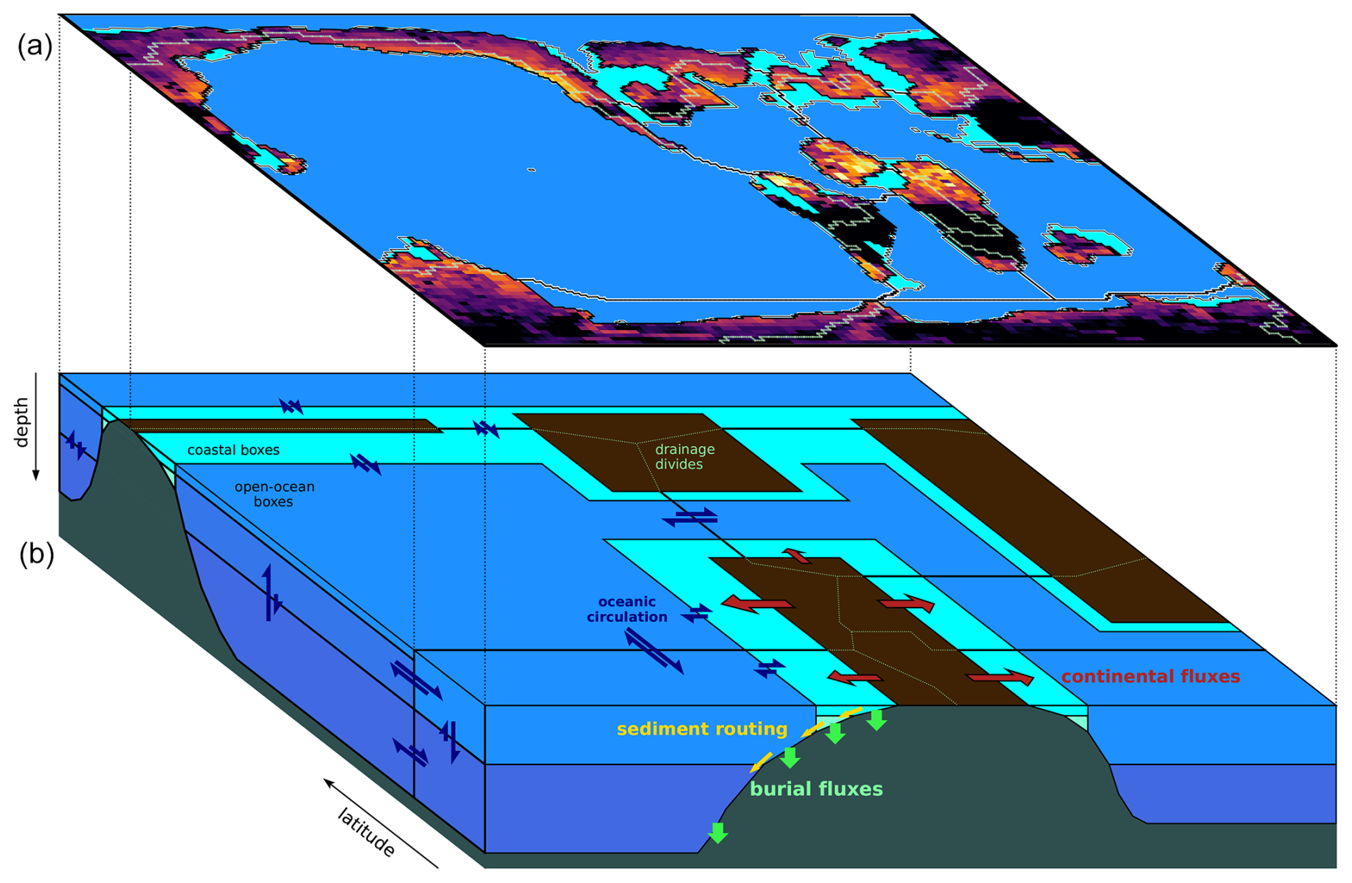
Figure 3 Schematics of GEOCLIM ocean and land discretization for the example of the Turonian configuration, with 28 oceanic boxes. The upper part (a) of the figure shows the paleogeographic map as represented by the GCM coupled with GEOCLIM (in this case, IPSL-CM5A2). The continental discretization is illustrated by the weathering map. The lower part (b) is a simplified representation of the oceanic basins, as integrated in GEOCLIM, depicting their main characteristics (latitudes, sizes, and connections). Note that the Southern Ocean and the Antarctic continent are not accurately represented for the sake of readability. Arrows for oceanic circulation, continental fluxes, sediment routing, and burial fluxes are not drawn for all concerned boxes and boundaries, also for the sake of readability.

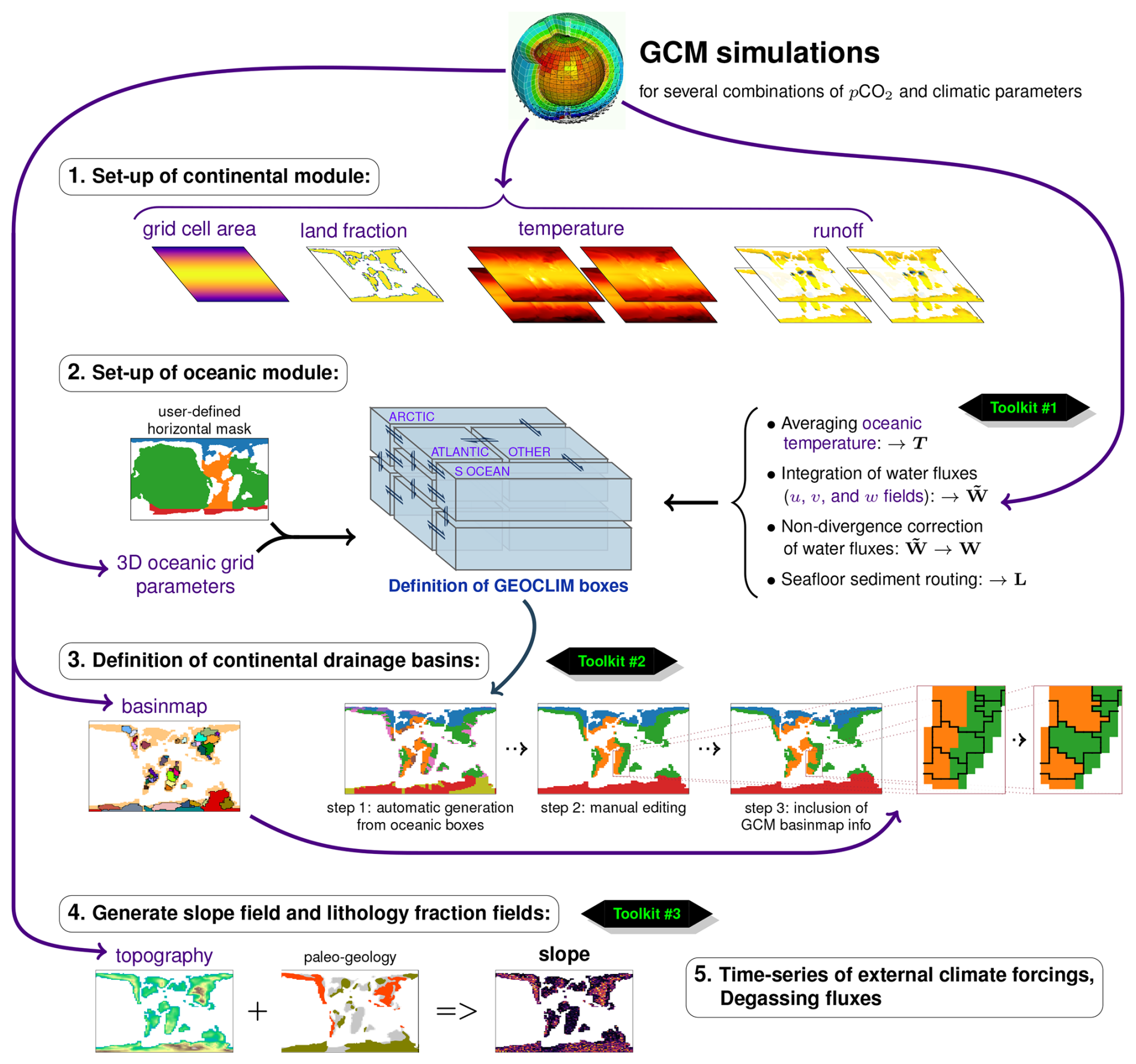
Figure 4 Summary of all the steps in the GEOCLIM setup. The “toolkits” mentioned in the figure are several sets of Python and Fortran scripts designed to generate the boundary condition files. Those scripts are stored in the following repertories of GEOCLIM's repository: preproc/BC/ (toolkit #1), preproc/BC/basinmap/ (toolkit #2), and preproc/ (toolkit #3). We note that paleogeology (an a priori information; cf. Sect. 3.4.1) could also be used to reconstruct the lithology fraction field, but this was not done in this study.

3.1 Connecting GCM land outputs to the weathering module

Because the continental module of GEOCLIM uses the same geographic resolution as the GCM connected to GEOCLIM, this configuration step only requires specifying which fields to use among the GCM outputs and generating the fields of topographic slope and lithology (see Sects. 3.4.1 and 3.4.2). The 2D geographic fields needed by the continental module are area and land fraction of the grid cells, surface air temperature, runoff (i.e., precipitation minus evaporation), topographic slope, and fraction of grid cells covered by each lithological class (Fig. 4). An additional optional input may be given: the global (land and ocean) field surface air temperature. This last input is only needed to compute global mean surface temperature, which is an offline variable (not needed for any calculation in GEOCLIM). It often differs from the continental air surface temperature field that excludes the ocean parts of “mixed” cells of the GCM grid. Therefore, this field is kept as a separate input. The temperature and runoff fields must be provided for all combinations of CO₂ levels and external climate forcings. If a different grid than the GCM is used, one must simply interpolate all the needed fields on the new grid, with any regridding method.

3.2 Connecting GCM ocean outputs to the oceanic module

While the connection of GCM outputs to the weathering module has been routinely done in several previous studies using GEOCLIM, oceanic fields used in the oceanic module were always kept to idealistic values as described above. Our goal is now to move forward by using oceanic fields as simulated by a coupled ocean–atmosphere GCM to force our oceanic box module. The methods presented in the current section therefore constitute an innovation of the present study (unless indicated otherwise). Defining and computing the characteristic of oceanic boxes is, however, less straightforward. A tool has been designed to make these definitions and computations from the “raw” 3D oceanic outputs of the GCM. It needs the following information: physical dimension of the GCM's oceanic grid (latitude, length, width, and depth of each cell), bathymetry, seawater temperature, and water horizontal velocity or fluxes between grid cells (the vertical velocity is optional). The temperature and velocity (or fluxes) must be provided for all combinations of CO₂ levels and external climate forcings.

The first step required to define oceanic boxes is to indicate cut-off depths of the vertical levels, the eventual cut-off latitudes, the seafloor depth separating coastal from open-ocean boxes, and an optional horizontal mask indicating the large-scale basins (e.g., Pacific, Atlantic, Indian). Those basins may include polar basins, making the latitude cut-off unnecessary. With this information, the coastal versus open-ocean splitting, the vertical splitting, and the (eventual) latitude splitting will be automatically performed for all the basins defined by the horizontal mask (if provided). An option is left to have a single, worldwide coastal box (always split into two vertical levels) or to have one coastal box per basin. By default, the first two levels are merged for high-latitude boxes. In other words, the first (shallower) cut-off depth is ignored for high-latitude boxes. This is meant to represent the deep mixed layer in places subject to deepwater formation. A full 3D mask in thus created to assign each cell of the GCM's 3D oceanic grid to its corresponding GEOCLIM box (Fig. 4). With that generated 3D mask, the characteristics of the boxes are calculated: volume (sum of the volume of the grid cells), top horizontal area (sum of areas of grid cells at the top of the box), horizontal area intercepting the seafloor (sum of areas of grid cells that are at the bottom of the water column), mean pressure (with hydrostatic approximation), and mean temperature (weighted average of seawater temperature). The last two variables computed from the GCM outputs are the “cross-level boundary length matrix” L and the water exchange matrix W.

L is computed as follows: for each pair of boxes i and j, L_ij is the sum of the lengths of the edges of all grid cells of box i that are at the bottom of the water column and that are adjacent to a cell in box j (only the edges connecting the cell in box i to the cell in box j are considered). The boundary-condition-generating tool computes L_ij for all combinations of i and j. The elements of L that do not follow its actual definition (L_ij>0 only if j is in a vertical level immediately below i; see Sect. 2.3.2) will be set to 0 during the initialization step of GEOCLIM.

To determine the water exchange matrix, the first step is to calculate the “naive” horizontal exchange matrix ${\stackrel{\mathrm{̃}}{\mathbf{W}}}^{\mathbf{h}}$. For each pair of boxes i and j (i≠j), the following holds.

$$\begin{array}{}\text{(93)}& {\displaystyle }\begin{array}{rl}{{\stackrel{\mathrm{̃}}{W}}^{\mathrm{h}}}_{ij}=& \sum _{x,y}u(x,y)\cdot min\left(A_{yz}(x,y),A_{yz}(x+dx,y)\right)\\ & \cdot {\mathbf{1}}_{u(x,y)>\mathrm{0}}\cdot {\mathbf{1}}_{\mathit{\{}x,y\mathit{\}}\in i}\cdot {\mathbf{1}}_{\mathit{\{}x+dx,y\mathit{\}}\in j}\\ -& \sum _{x,y}u(x,y)\cdot min\left(A_{yz}(x,y),A_{yz}(x+dx,y)\right)\\ & \cdot {\mathbf{1}}_{u(x,y)<\mathrm{0}}\cdot {\mathbf{1}}_{\mathit{\{}x+dx,y\mathit{\}}\in i}\cdot {\mathbf{1}}_{\mathit{\{}x,y\mathit{\}}\in j}\\ +& \sum _{x,y}v(x,y)\cdot min\left(A_{xz}(x,y),A_{xz}(x,y+dy)\right)\\ & \cdot {\mathbf{1}}_{v(x,y)>\mathrm{0}}\cdot {\mathbf{1}}_{\mathit{\{}x,y\mathit{\}}\in i}\cdot {\mathbf{1}}_{\mathit{\{}x,y+dy\mathit{\}}\in j}\\ -& \sum _{x,y}v(x,y)\cdot min\left(A_{xz}(x,y),A_{xz}(x,y+dy)\right)\\ & \cdot {\mathbf{1}}_{v(x,y)<\mathrm{0}}\cdot {\mathbf{1}}_{\mathit{\{}x,y+dy\mathit{\}}\in i}\cdot {\mathbf{1}}_{\mathit{\{}x,y\mathit{\}}\in j}\end{array}\end{array}$$

Here, u and v are the oceanic velocity in the x and y direction (respectively), A_yz and A_xz are the vertical areas of a grid cell in the (y,z) and (x,z) Euclidean planes (respectively), 1_* is the indicator function (=1 if condition * is verified, 0 otherwise), and “$\mathit{\{}x,y\mathit{\}}\in i$” means “grid cell {x,y} is in box i”. dx and dy are the spatial increments and simply mean here that x and x+dx are adjacent (and similarly for y). Equation (93) considers a configuration with an Arakawa C-type “staggered” grid: u(x,y), representing the velocity between {x,y} and $\mathit{\{}x+dx,y\mathit{\}}$, is positioned at $\mathit{\{}x+dx/\mathrm{2},y\mathit{\}}$, and similarly, v(x,y), representing the velocity between {x,y} and $\mathit{\{}x,y+dy/\mathrm{2}\mathit{\}}$, is positioned at $\mathit{\{}x,y+dy/\mathrm{2}\mathit{\}}$. This configuration is common for GCM oceanic components and is, in particular, the one of IPSL-CM5A2 (NEMO-ORCA2, Sepulchre et al., 2020) used for this study. As a consequence, the minimum of vertical areas is considered in the computation of horizontal water fluxes because two adjacent cells may have different vertical areas if they intercept bathymetry at different depths. In such a case, the minimum vertical area should be used to compute the fluxes between the cells. If the water flux between grid cells is present in the oceanic outputs of the GCM, instead of oceanic velocity, it can be used in Eq. (93) as a replacement for “velocity times vertical area”. The computation of ${\stackrel{\mathrm{̃}}{\mathbf{W}}}^{\mathbf{h}}$ (just like the computation of L) must account for specific boundary conditions, like periodic x boundary conditions (often encountered, with x being longitude or assimilated), or special cases like the north fold of the tripolar oceanic grid of IPSL-CM5A2.

The vertical exchange matrix ${\stackrel{\mathrm{̃}}{\mathbf{W}}}^{\mathbf{v}}$ could be computed following the method of Eq. (93), with w and A_xy, but this method is highly inaccurate. Indeed, vertical velocity in a GCM is almost systematically diagnosed from the divergence of horizontal velocity and is often noisy, with alternating positive and negative velocities from cell to cell. Summing those ups and downs would generate a large overestimation of vertical mixing, of more than an order of magnitude. To avoid this issue, we opted for deducing net vertical exchanges between boxes from the horizontal divergence of ${\stackrel{\mathrm{̃}}{\mathbf{W}}}^{\mathbf{h}}$ and adding a constant bidirectional vertical velocity w_mix, meant to represent turbulent mixing of the water column. w_mix is set to $\mathrm{8}\times {\mathrm{10}}^{-\mathrm{8}}$ m s⁻¹, which yields a worldwide vertical turbulent mixing flux of ∼30 Sv, with that value being tuned to obtain a consistent age model, with the oldest deepwater age of ∼1000 years. ${\stackrel{\mathrm{̃}}{\mathbf{W}}}^{\mathbf{v}}$ is computed iteratively, from the top to the bottom of each water column. Keeping in mind that GEOCLIM's boxes are ordered in such way that box i+1 is below box i, unless box i is at the bottom of the water column, for each surface box i₀, the following holds.

$$\begin{array}{ll}{\displaystyle }& {\displaystyle }\text{if }\sum _k({{\stackrel{\mathrm{̃}}{W}}^{\mathrm{h}}}_{k,i_{\mathrm{0}}}-{{\stackrel{\mathrm{̃}}{W}}^{\mathrm{h}}}_{i_{\mathrm{0}},k})>\mathrm{0}:\\ {\displaystyle }& {\displaystyle }\left\{\begin{array}{rl}{\displaystyle }{{\stackrel{\mathrm{̃}}{W}}^{\mathrm{v}}}_{i_{\mathrm{0}},i_{\mathrm{0}}+\mathrm{1}}& {\displaystyle }=w_{\text{mix}}{A}_{i_{\mathrm{0}}+\mathrm{1}}+\sum _k({{\stackrel{\mathrm{̃}}{W}}^{\mathrm{h}}}_{k,i_{\mathrm{0}}}-{{\stackrel{\mathrm{̃}}{W}}^{\mathrm{h}}}_{i_{\mathrm{0}},k})\\ {\displaystyle }{{\stackrel{\mathrm{̃}}{W}}^{\mathrm{v}}}_{i_{\mathrm{0}}+\mathrm{1},i_{\mathrm{0}}}& {\displaystyle }=w_{\text{mix}}{A}_{i_{\mathrm{0}}+\mathrm{1}}\end{array}\right.\\ {\displaystyle }& {\displaystyle }\text{otherwise:}\\ \text{(94)}& {\displaystyle }& {\displaystyle }\left\{\begin{array}{rl}{\displaystyle }{{\stackrel{\mathrm{̃}}{W}}^{\mathrm{v}}}_{i_{\mathrm{0}},i_{\mathrm{0}}+\mathrm{1}}& {\displaystyle }=w_{\text{mix}}{A}_{i_{\mathrm{0}}+\mathrm{1}}\\ {\displaystyle }{{\stackrel{\mathrm{̃}}{W}}^{\mathrm{v}}}_{i_{\mathrm{0}}+\mathrm{1},i_{\mathrm{0}}}& {\displaystyle }=w_{\text{mix}}{A}_{i_{\mathrm{0}}+\mathrm{1}}-\sum _k({{\stackrel{\mathrm{̃}}{W}}^{\mathrm{h}}}_{k,i_{\mathrm{0}}}-{{\stackrel{\mathrm{̃}}{W}}^{\mathrm{h}}}_{i_{\mathrm{0}},k})\end{array}\right.\end{array}$$

Then, for all the following boxes, the following holds.

$$\begin{array}{}\text{(95)}& {\displaystyle }\begin{array}{rl}\text{if }& ({{\stackrel{\mathrm{̃}}{W}}^{\mathrm{v}}}_{i_{\mathrm{0}},i_{\mathrm{0}}+\mathrm{1}}-{{\stackrel{\mathrm{̃}}{W}}^{\mathrm{v}}}_{i_{\mathrm{0}}+\mathrm{1},i_{\mathrm{0}}})\\ & +\sum _k({{\stackrel{\mathrm{̃}}{W}}^{\mathrm{h}}}_{k,i_{\mathrm{0}}+\mathrm{1}}-{{\stackrel{\mathrm{̃}}{W}}^{\mathrm{h}}}_{i_{\mathrm{0}}+\mathrm{1},k})>\mathrm{0}:\\ & \left\{\begin{array}{rl}{\stackrel{\mathrm{̃}}{W}}^{\mathrm{v}}& {}_{i_{\mathrm{0}}+\mathrm{1},i_{\mathrm{0}}+\mathrm{2}}=w_{\text{mix}}{A}_{i_{\mathrm{0}}+\mathrm{2}}\\ & +({{\stackrel{\mathrm{̃}}{W}}^{\mathrm{v}}}_{i_{\mathrm{0}},i_{\mathrm{0}}+\mathrm{1}}-{{\stackrel{\mathrm{̃}}{W}}^{\mathrm{v}}}_{i_{\mathrm{0}}+\mathrm{1},i_{\mathrm{0}}})\\ & +\sum _k({{\stackrel{\mathrm{̃}}{W}}^{\mathrm{h}}}_{k,i_{\mathrm{0}}+\mathrm{1}}-{{\stackrel{\mathrm{̃}}{W}}^{\mathrm{h}}}_{i_{\mathrm{0}}+\mathrm{1},k})\\ {\stackrel{\mathrm{̃}}{W}}^{\mathrm{v}}& {}_{i_{\mathrm{0}}+\mathrm{2},i_{\mathrm{0}}+\mathrm{1}}=w_{\text{mix}}{A}_{i_{\mathrm{0}}+\mathrm{2}}\end{array}\right.\\ & \text{otherwise:}\\ & \left\{\begin{array}{rl}{\stackrel{\mathrm{̃}}{W}}^{\mathrm{v}}& {}_{i_{\mathrm{0}}+\mathrm{1},i_{\mathrm{0}}+\mathrm{2}}=w_{\text{mix}}{A}_{i_{\mathrm{0}}+\mathrm{2}}\\ {\stackrel{\mathrm{̃}}{W}}^{\mathrm{v}}& {}_{i_{\mathrm{0}}+\mathrm{2},i_{\mathrm{0}}+\mathrm{1}}=w_{\text{mix}}{A}_{i_{\mathrm{0}}+\mathrm{2}}\\ & -({{\stackrel{\mathrm{̃}}{W}}^{\mathrm{v}}}_{i_{\mathrm{0}},i_{\mathrm{0}}+\mathrm{1}}-{{\stackrel{\mathrm{̃}}{W}}^{\mathrm{v}}}_{i_{\mathrm{0}}+\mathrm{1},i_{\mathrm{0}}})\\ & -\sum _k({{\stackrel{\mathrm{̃}}{W}}^{\mathrm{h}}}_{k,i_{\mathrm{0}}+\mathrm{1}}-{{\stackrel{\mathrm{̃}}{W}}^{\mathrm{h}}}_{i_{\mathrm{0}}+\mathrm{1},k})\end{array}\right.\\ & \mathrm{\dots }\end{array}\end{array}$$

And so on until the bottom of the water column starting at box i₀ is reached.

The “full” water exchange matrix $\stackrel{\mathrm{̃}}{\mathbf{W}}$ is simply the sum of the horizontal and vertical components: $\stackrel{\mathrm{̃}}{\mathbf{W}}={\stackrel{\mathrm{̃}}{\mathbf{W}}}^{\mathbf{h}}+{\stackrel{\mathrm{̃}}{\mathbf{W}}}^{\mathbf{v}}$. The method of Eqs. (94) and (95) ensures that $\stackrel{\mathrm{̃}}{\mathbf{W}}$ is non-divergent (${\sum }_k{\stackrel{\mathrm{̃}}{W}}_{ik}-{\stackrel{\mathrm{̃}}{W}}_{ki}=\mathrm{0}$) for every box i except the bottom ones. If the water column is non-divergent in the GCM's oceanic velocity fields, the bottom boxes will also have no water flux divergence, but it may not always be the case. For this reason, an additional corrective step is performed by the boundary-condition-generating script. A multiplicative correction matrix ϕ is applied so that the corrected water exchange matrix W (defined as $W_{ij}={\mathit{\varphi }}_{ij}{\stackrel{\mathrm{̃}}{W}}_{ij}$) is non-divergent everywhere. ϕ is computed with a least-square approach. It is fully defined by the following conditions.

$$\begin{array}{ll}{\displaystyle }& {\displaystyle }\sum _k({\mathit{\varphi }}_{ik}{\stackrel{\mathrm{̃}}{W}}_{ik}-{\mathit{\varphi }}_{ki}{\stackrel{\mathrm{̃}}{W}}_{ki})=\mathrm{0}\forall i\\ \text{(96)}& {\displaystyle }& {\displaystyle }\sum _i\sum _j(\mathrm{1}-{\mathit{\varphi }}_{ij}{)}^{\mathrm{2}}\text{ is minimum}\end{array}$$

Equation (96) is a constrained optimization problem and is solved by a Lagrange multiplier method. The resolution is detailed in Appendix B2. This method is not always stable because it requires a numerical matrix inversion (see Appendix B2) and can lead to an improper solution, where the non-divergence condition is not fulfilled. This is, for instance, the case when the ocean has multiple unconnected clusters of boxes. If the multiplicative correction cannot be computed, an additive correction, which has no stability issue, is performed: $\mathbf{W}=\stackrel{\mathrm{̃}}{\mathbf{W}}+\mathit{\delta }$, with δ defined such as

$$\begin{array}{ll}{\displaystyle }& {\displaystyle }\sum _k({\stackrel{\mathrm{̃}}{W}}_{ik}+{\mathit{\delta }}_{ik}-{\stackrel{\mathrm{̃}}{W}}_{ki}-{\mathit{\delta }}_{ki})=\mathrm{0}\forall i\\ \text{(97)}& {\displaystyle }& {\displaystyle }\sum _i\sum _j{{\mathit{\delta }}_{ij}}^{\mathrm{2}}\text{ is minimum}.\end{array}$$

Equation (97) is also a constrained optimization problem and is solved by a Lagrange multiplier method. The resolution is detailed in Appendix B1. A last correction step is needed because this additive correction method can generate negative values in W, which has no physical meaning in the way advection equations are written. If W_ij<0, we simply add −W_ij to W_ji and set W_ij to 0.

The multiplicative correction method should always be preferred to the additive one because of its better properties: flux corrections are made relative to their absolute value, whereas with the additive method, a small correction, if added to an even smaller flux, is a major relative change. As a corollary, null fluxes will stay null with the multiplicative correction, whereas the additive correction can create fluxes between boxes that are not connected. The last correction step of the additive correction method, to avoid negative fluxes, is somewhat arbitrary (because that constraint cannot be easily added to the optimization problem) and breaks the least-square condition.

Finally, there are alternative options if the characteristics of oceanic boxes cannot all be deduced from the GCM's output. Box dimensions (volumes, horizontal areas) and mean pressures may be defined “by hand” or kept at GEOCLIM's default pre-industrial values (if the default 10-box configuration is used). Lateral sediment advection can be computed without the matrix L (see Sect. 2.3.2). The water exchange matrix can be kept at GEOCLIM's default pre-industrial values, still if the default 10-box configuration is used, and can always be defined as constant, i.e., not varying with CO₂ and external climate forcings. As for the oceanic temperature of GEOCLIM boxes, an option allows parameterizing them with a log (CO₂) fit that was derived from the oceanic temperature of a FOAM pre-industrial climate simulation (Donnadieu et al., 2006):

$$\begin{array}{l}{\displaystyle }\begin{array}{rl}& T=\mathrm{293.15}+\mathrm{4.88504}\cdot \log \left({\displaystyle \frac{p{{\mathrm{CO}}_{\mathrm{2}}}^{\text{atm}}}{{\left.p{{\mathrm{CO}}_{\mathrm{2}}}^{\text{atm}}\right|}_{\text{PI}}}}\right)\\ & \text{for coastal boxes and midlatitude surface boxes and}\end{array}\\ \text{(98)}& {\displaystyle }\begin{array}{rl}& T=\mathrm{266.56103}+\mathrm{6.89026}\cdot \log \left({\displaystyle \frac{p{{\mathrm{CO}}_{\mathrm{2}}}^{\text{atm}}}{{\left.p{{\mathrm{CO}}_{\mathrm{2}}}^{\text{atm}}\right|}_{\text{PI}}}}\right)\\ & \text{for deep boxes and high-latitude boxes}.\end{array}\end{array}$$

The new methods presented in this section were applied in all GEOCLIM simulations presented in this article. In Sect. 4.3, we show different configurations of GEOCLIM boxes. The differences between the default pre-industrial flux matrix and the one computed from IPSL-CM5A2 pre-industrial oceanic velocity fields are presented in Appendix C.

3.3 Connecting weathering module to the oceanic module: water routing

If GEOCLIM oceanic discretization is defined with a single surface coastal box (coastal boxes are always split into two vertical levels), the continental fluxes are integrated over the entire continents and sent to the surface coastal box:

$$\begin{array}{}\text{(99)}& F_{\left(i\right)}=\underset{\text{continents}}{\iint }\stackrel{,,}{F}\mathrm{d}x\mathrm{d}y,\end{array}$$

with i being the unique surface coastal box and F any flux computed by the continental module ($\stackrel{,,}{F}$ is the specific flux).

If, however, there is more than one surface coastal box, a water-routing scheme should be defined. The possibility to define multiple coastal boxes and the water-routing scheme are innovations of the present study. Another boundary-condition-generating tool was developed to generate the routing scheme semiautomatically. This Python script uses the definition of the land/atmosphere and oceanic grid of the GCM – which are often two different grids – to determine on each land grid point the closest ocean grid point and uses the 3D mask of GEOCLIM boxes (see Sect. 3.2) to assign a GEOCLIM box to each land grid point (Fig. 4). This yields a first guess of a water-routing mask. That mask is then left to be interactively edited by the user, which is needed for two reasons: firstly, the algorithm may find open-ocean boxes as the closest oceanic point because on some coast, bathymetry drops too fast to significant depth, and the “shallow” points are invisible at the GCM's resolution. This needs to be manually edited to replace all open-ocean boxes by the corresponding coastal box. Secondly, this guess ignores all information about hydrographic networks that may be implemented in the GCM. The user thus has the possibility to load the map of river basins used by the GCM into the interactive editor and select the river basins that go into each GEOCLIM box drainage basin (hereafter called “watersheds”). Figure 3 illustrates the water-routing scheme, showing the drainage divides at the continental resolution (i.e., the resolution of IPSL climate model) and schematized for GEOCLIM boxes. The continental fluxes going into each coastal surface box i are then the integral of the specific fluxes over the watershed thus defined:

$$\begin{array}{}\text{(100)}& F_{\left(i\right)}=\underset{\text{watershed}i}{\iint }\stackrel{,,}{F}\mathrm{d}x\mathrm{d}y,\end{array}$$

with a special case for phosphorus fluxes (see Sect. 2.4.7, Eqs. 91 and 92).

An alternative option available in GEOCLIM is to integrate the continental fluxes over the entire continents (Eq. 99) and to distribute them on every coastal surface box i on a pro rata basis of their surface areas A_i.

3.4 Other boundary conditions

This section describes the boundary conditions needed by GEOCLIM that cannot be directly deduced from the GCM outputs.

3.4.1 Topographic slope

The field of topographic slope needed by GEOCLIM's continental module DynSoil (Eq. 75) is the gradient of high-resolution topography, averaged at the continental resolution of GEOCLIM (a few degrees of longitude and latitude). If computed at that latter resolution, the gradient of topography would be largely underestimated because of the smoothing of topography. For modern slope field, we used the SRTM topography field at 30^′′ (∼0.0083°) resolution to compute the gradient and averaged it at the desired resolution. For paleogeographic reconstruction, such high-resolution topography cannot be known, so the slope must be deduced from lower-resolution data.

We present h a new nonparametric method to reconstruct the slope, guided by topography and first-order geological settings of a given paleogeography (Fig. 4). Continental points (both modern and paleo, at the same grid resolution) are classified into broad geological categories (e.g., active orogens, ancient orogens, and the rest of the continents) and elevation range categories (e.g., 0–500 m, 500–1000 m, 1000–2000 m, and >2000 m). Then, for each point of the paleocontinental grid, we randomly pick a slope value from a point of the modern continental grid that is in the same geological and elevation category. This method ensures that, for each geology–elevation category, the paleo-slope distribution is (statistically) the same as the modern one.

3.4.2 Lithology

Other information needed by GEOCLIM's continental module is the fraction of each continental grid cell covered by each lithological class (that is a 3D field, $n_x\times n_y\times N_{\text{litho}}$, with (n_x,n_y) the size of the 2D grid and N_litho the number of classes; see Sect. 2.4 for the standard lithological categories). To compute the modern field of lithology fraction, we rasterized the polygons of the lithology database of Hartmann and Moosdorf (2012) for each of our lithological classes. The addition of lithological information has been implemented and tested in “GEOCLIM-DynSoil-steady state” by Park et al. (2020) and was already used in Maffre et al. (2021). In the case of paleogeographic reconstruction, the lithology fraction can be deduced if the reconstruction includes paleogeology or using the same broad geological categories as for slope by analogy with lithology assemblages of the modern geological categories. Otherwise, a neutral assumption is to impose a uniform lithology using the modern global mean lithology fractions.

3.4.3 External climate forcings

GEOCLIM can take into account the effect of external climate forcings that can be represented by a unique scalar value. This feature is a novelty of the present contribution. External climate forcings are processes influencing climate fields without any feedback from climate and biogeochemical cycles. The canonical example of external climate forcing that we present in this article is Milanković parameters: the Earth's axis tilt (obliquity), the eccentricity of Earth' orbit around the sun, and the position of perihelion in the seasonal cycle (precession angle ω). If external climate forcings are “activated”, GEOCLIM reads their scalar values from a time series in a text file at a reading time step indicated in the configuration file (each line of the file being a time step, the first line corresponding to the start of the run). Between two reading time steps, the values of external climate forcings are linearly interpolated. Those values are used to generate the climatic fields corresponding to the current combination of pCO₂ and external climate forcings by multilinear interpolation between the input fields (themselves coming from climate simulations conducted with different combinations of pCO₂ and external climate forcings, also indicated in the GEOCLIM configuration file). External climate forcings with periodic values – like the precession angle, ranging from 0 to 360° – must also be indicated. In the source code of GEOCLIM, the external climate forcings are called “climatic parameters”.

3.4.4 Degassing fluxes

Four CO₂ degassing fluxes are imposed to the model by the user (in a configuration file): from subaerial volcanics ($F_{\text{volc}}^{{\mathrm{CO}}_{\mathrm{2}}}$, used in Eqs. 2 and 20), from mid-oceanic ridges ($F_{\text{MOR}}^{{\mathrm{CO}}_{\mathrm{2}}}$, used in Eqs. 1, 17, and 19) as distributed by the code in the deep oceanic boxes, from trap volcanism ($F_{\text{trap}}^{{\mathrm{CO}}_{\mathrm{2}}}$, used in Eqs. 2 and 20), and from anthropogenic forcing ($F_{\text{anth}}^{{\mathrm{CO}}_{\mathrm{2}}}$, used in Eqs. 2, 7, and 20). The first two are constant background fluxes, while the last two are time-evolving fluxes, following a prescribed scenario.

In the standard configuration of GEOCLIM, $F_{\text{trap}}^{{\mathrm{CO}}_{\mathrm{2}}}$ and $F_{\text{anth}}^{{\mathrm{CO}}_{\mathrm{2}}}$ are null. The total background degassing $F_{\text{volc}}^{{\mathrm{CO}}_{\mathrm{2}}}+F_{\text{MOR}}^{{\mathrm{CO}}_{\mathrm{2}}}$ is determined, for pre-industrial conditions, by equalizing the silicate weathering flux $F_{\text{silw}}+x_{\text{sil}}^{\text{sulw}}{F}_{\text{sulw}}$ (i.e., from both carbonic and sulfuric acid) at a pCO₂ of 280 µatm, thus assuming steady state of all geochemical cycles. Paleo total background degassing may be taken from reconstruction of relative degassing with respect to pre-industrial or may be tuned in order to reach a pCO₂ or sea surface temperature (SST) consistent with proxies. By default, the relative contribution of mid-ocean ridge degassing to the total flux is 0.119.

3.5 Model calibration

GEOCLIM was calibrated to reproduce pre-industrial conditions with a “control” run using IPSL-CM5A2 climate fields. The only exception is DynSoil (the silicate weathering module), whose parameters were calibrated by Park et al. (2020) to fit modern observations of silicate weathering flux in 80 river basins. We did not modify these parameters for the present study, even though different climate fields were used (IPSL climate outputs versus ERA5 reanalysis in Park et al., 2020), leading to slightly different distributions of weathering rates and global weathering flux.

3.5.1 Pre-industrial climate fields

The control run of GEOCLIM was performed with the standard 10-box configuration (see Sect. 2.2.1 and Fig. 1), but with a deep box depth cut-off at 900 m (instead of 1000 m), a southern high-latitude cut-off at 65° S (instead of 60° S), and a northern high-latitude mask that includes the North Atlantic (around 59° N) but excludes the North Pacific. These choices were made to capture as accurately as possible the global oceanic circulation within the IPSL-CM5A2 climate outputs, with North Atlantic deepwater formation and bottom water formation south of 65° S, while upwellings from the Antarctic Circumpolar Current are north of 65° S. The oceanic circulation, as well as ocean temperature, continental temperature, and runoff, comes from a coupled ocean–atmosphere pre-industrial simulation with the IPSL-CM5A2 climate model, following the integration method presented in Sects. 3.1 and 3.2. That IPSL-CM5A2 simulation was published in Laugié et al. (2020), though the model itself was published by Sepulchre et al. (2020). It was conducted with standard pre-industrial climate model forcings at a horizontal resolution of 3.75°×1.875° (longitude × latitude) for atmosphere and land and a curvilinear oceanic grid with an approximated horizontal resolution of 2° with refinement to 0.5° around the Equator, as well as variable depth resolution (from 10 m near the surface to 500 m near the bottom). The climate simulation was run for 1800 years, and the last 100 years were averaged to generate the annual mean climatology.

3.5.2 Tuning of continental fluxes

With Park et al. (2020)'s parameters and IPSL-CM5A2 climate fields, the global silicate weathering flux is 3.55 Tmol yr⁻¹. The carbonate weathering parameter k_carb was tuned so that the global carbonate weathering flux is 12.3 Tmol yr⁻¹ (Gaillardet et al., 1999).

We kept the values of χ_foc and χ_S from Maffre et al. (2021), as well as the values of $x_{\text{carb}}^{\text{sulw}}$ and $x_{\text{sil}}^{\text{sulw}}$. They were meant to achieve a global petrogenic carbon oxidation flux of 5.0 Tmol yr⁻¹ (Lenton et al., 2018) and a global sulfide weathering flux of 1.3 Tmol yr⁻¹ (Burke et al., 2018). A more recent estimation of petrogenic carbon oxidation from Zondervan et al. (2023) gives a value of ${\mathrm{5.6}}_{-\mathrm{0.5}}^{+\mathrm{1.5}}$ Tmol yr⁻¹. With IPSL climate fields, GEOCLIM's petrogenic carbon oxidation and sulfide weathering fluxes are 4.61 and 1.20 Tmol yr⁻¹ (respectively).

Once all the other continental fluxes were set, the C:P ratio of fossil organic carbon was left at the value of Goddéris and Joachimski (2004). The C:P ratio corresponding to the uptake by the continental biosphere ((C:P)_cont) was set to 205 (Maffre et al., 2021). Finally, the amount of P in silicate and carbonate lithology (χ_P) was taken from Hartmann et al. (2014), simply modifying the value in sediment so that the global P weathering fluxes in dissolved form ($F_{\text{diss}}^{\mathrm{P}\mathrm{w}}$) and associated with exported terrestrial POC ($F_{\text{part}}^{\mathrm{P}\mathrm{w}}$) are consistent with Filippelli (2002). GEOCLIM's dissolved and POC-associated P fluxes are 29.3 and 47.4 Gmol yr⁻¹ (respectively), while Filippelli (2002) estimated a dissolved P flux of 1 Pg yr⁻¹ (32 Gmol yr⁻¹) and a “soluble” P flux of 1–2 Pg yr⁻¹ (32–64 Gmol yr⁻¹).

3.5.3 Tuning of ocean–atmosphere geochemistry

Because of the interdependency of the biogeochemical processes, the calibration was conducted in the following order, after calibration of continental fluxes.

The constant for sediment accumulation capacity k_sed was tuned to achieve a realistic distribution of sedimentation rates in the GEOCLIM control run: 20–25 cm yr⁻¹ in coastal boxes, ∼15 cm yr⁻¹ in intermediate boxes, and 0.3–2 cm yr⁻¹ in deep boxes. There is not much liberty in this tuning since there is only one parameter for nine boxes. Moreover, there is a trade-off since the global sedimentation flux is largely determined by the continental erosion flux (pCO₂ is held constant at the pre-industrial value for this tuning so that the erosion flux is also constant). Hence, adjusting k_sed to increase the sedimentation of coastal boxes would automatically reduce the sedimentation rate of deep boxes.

The following parameters were tuned holding pCO₂, pO₂, and mean $\left[{\mathrm{SO}}_{\mathrm{4}}^{\mathrm{2}-}\right]$ constant at pre-industrial values. The first step is to set the global degassing flux ($F_{\text{volc}}^{{\mathrm{CO}}_{\mathrm{2}}}+F_{\text{MOR}}^{{\mathrm{CO}}_{\mathrm{2}}}$) equal to the sum of global carbonic and sulfuric silicate weathering ($F_{\text{silw}}+x_{\text{sil}}^{\text{sulw}}{F}_{\text{sulw}}$) corresponding to pre-industrial pCO₂. Indeed, this condition ultimately sets the equilibrium pCO₂, once all the other geochemical cycles are at steady state.

Then, the sum of the two constant k_P hyd+k_P ite determines the inorganic P sink (i.e., the sink that is independent of organic C sink) and therefore has the most direct control on the amount of P left in the ocean and available for primary productivity. Thus, we tuned k_P hyd+k_P ite so that the net global primary productivity of the photic zone – which, at steady state, is equal to the export of organic C below the photic zone – is within 400–1000 Tmol yr⁻¹ (Andersson et al., 2004; Dunne et al., 2007; Henson et al., 2011; Siegel et al., 2014; DeVries and Weber, 2017; Sulpis et al., 2023). Note that the individual values of k_P hyd and k_P ite do not matter; only the sum does (see Eqs. 72 and 73).

With the global primary productivity flux set, the sinking rate of particles w_sink and POC remineralization constant k_oxyd were jointly tuned in order to achieve a realistic distribution of dissolved oxygen, with an open-ocean minimum in the midlatitude intermediate depth box (see Fig. 5c2). There is a degree of liberty in these two parameters: at steady state, a combination of high sinking rate and high remineralization constant will give the same vertical profiles as another combination of low sinking rate and low remineralization constant. Both of those parameters are poorly constrained, except for the technical constraint – though somewhat artificial – that an overly high w_sink would generate numerical instabilities.

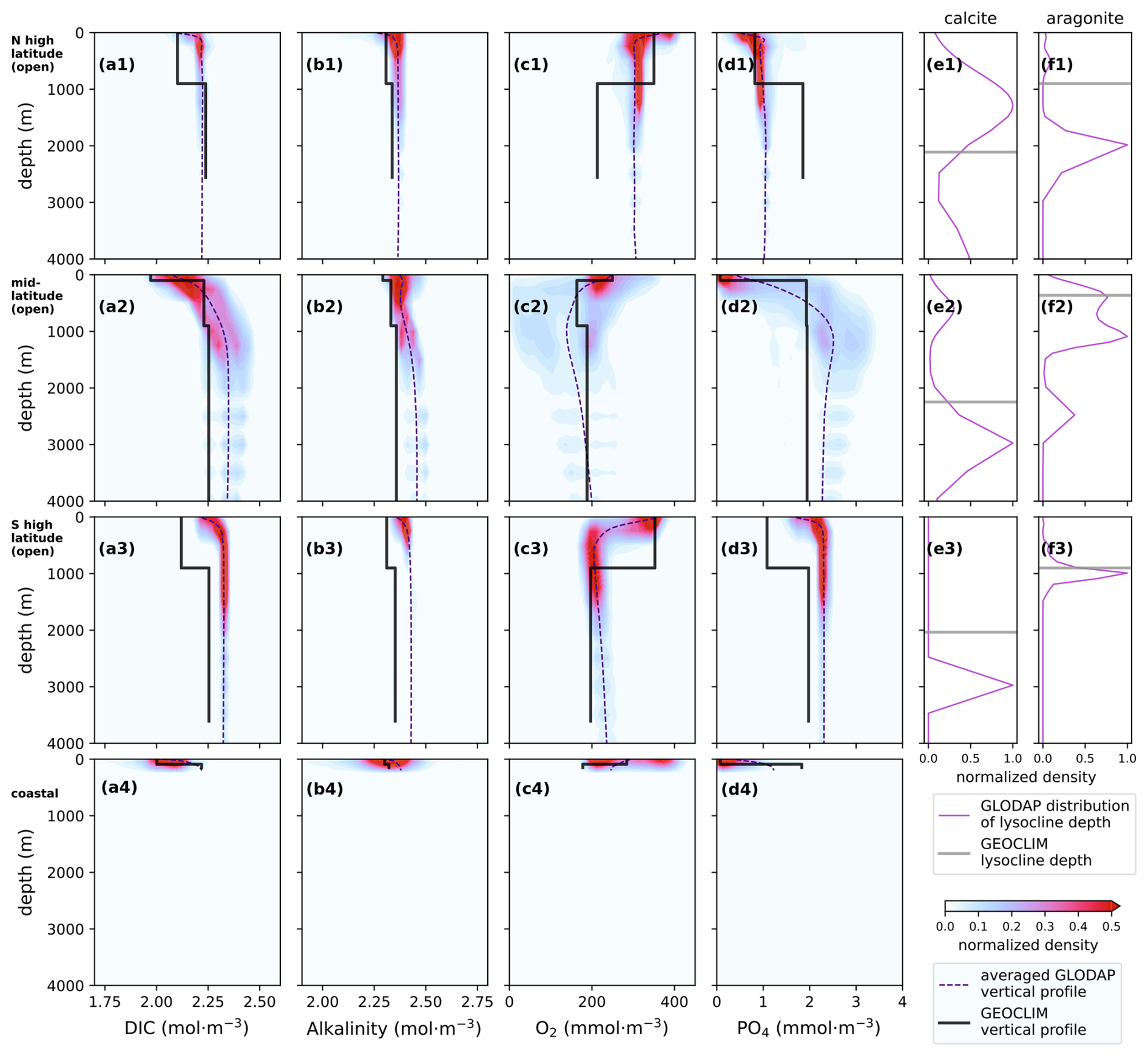
Figure 5 Vertical profiles of the main geochemical variables of the pre-industrial control GEOCLIM simulation at steady state (last time step of the simulation) and modern observations from the GLODAPv2 database. (a1–a4) DIC concentration, (b1–b4) alkalinity, (c1–c4) O₂ concentration, (d1–d4) P concentration, (e1–e3) calcite lysocline depth (vertical level), (f1–f3) aragonite lysocline depth. Each line represents a “column” of GEOCLIM boxes: 1. northern high latitudes (boxes #1 and 2), 2. midlatitudes (boxes #3, 4 and 5), 3. southern high latitudes (boxes #8 and 9), 4. coastal boxes (#6 and 7). GLODAPv2 data are shown as value–depth 2D kernel density estimates normalized by the maximum density (color shadings), horizontal averages (purple dashed lines), and distributions of lysocline depths (purple solid lines).

With primary productivity and the oxygen profile set, we tuned x_shell (broadly representing the fraction of calcifying primary producers) so that the global net carbonate productivity (both open water and reef carbonates) is ∼50 Tmol yr⁻¹ (literature estimates span 50 to 130 Tmol yr⁻¹; Dunne et al., 2007; Berelson et al., 2007; Smith and Mackenzie, 2016; Sulpis et al., 2021). We then tuned k_diss and k_reef to achieve a realistic carbonate chemistry: a surface alkalinity within 2.3–2.4 mol m⁻³, a surface pH around 8.2, and calcite lysocline depth within 2000–3000 m (see Fig. 5). k_reef directly controls reef carbonate precipitation. Together with x_shell – whose value in coastal oceanic boxes was adjusted (see Sect. 2.2.4) – they determine the distribution of carbonate precipitation in the coastal ocean versus in open ocean. With the current tuning, ∼40 % of the global carbonate burial takes place in the coastal ocean, and ∼30 % of the global burial flux is reef carbonate. There was some back-and-forth with the parameters mentioned in the previous paragraph. We found it necessary to lower the net global primary productivity flux to ∼420 Tmol yr⁻¹ (by adjusting k_P hyd+k_P ite) to conciliate a global mean alkalinity not higher than 2.5 mol m⁻³ and calcite lysocline depths not shallower than 2000 m.

Finally, once all the abovementioned parameters were set, we relaxed the constraint of pO₂ and $\left[{\mathrm{SO}}_{\mathrm{4}}^{\mathrm{2}-}\right]$ and let the oxygen and sulfur cycles behave “freely”. We then jointly tuned the parameters k_ml and k_sr so that the organic C burial flux and the sulfate reduction flux balance the petrogenic organic C and sulfide weathering fluxes (respectively). The implicit assumption behind this tuning is that oxygen and sulfur cycles are at steady state with pre-industrial conditions. Because of the intertwining of oxygen and sulfur fluxes, k_ml and k_sr must be adjusted simultaneously, with a series of trials and errors, until both pO₂ and mean $\left[{\mathrm{SO}}_{\mathrm{4}}^{\mathrm{2}-}\right]$ are stabilized at pre-industrial values. This tuning does affect oceanic oxygen and carbonate chemistry because of the oxygen, DIC, and alkalinity fluxes from the sediment to the ocean. However, those fluxes are 1 or 2 orders of magnitude smaller than the fluxes of organic primary productivity, carbonate productivity, water column POC remineralization, and PIC dissolution, so the tuning of k_ml and k_sr only has a second-order effect on the calibrated profiles of oxygen, alkalinity, pH and lysocline depth.

Figure 5 shows the vertical profiles of this tuned pre-industrial steady-state GEOCLIM simulation in each vertical “column” of GEOCLIM oceanic discretization (see also Sect. 2.2.1). The modern observations, extracted from the GLODAPv2 database (Lauvset et al., 2023; Olsen et al., 2016; Lauvset et al., 2016), are superimposed in Fig. 5 after being horizontally averaged on GEOCLIM's “columns” (dashed lines). The distribution within each column is also shown (color shadings). GEOCLIM reproduced the horizontally averaged vertical gradients relatively well, keeping in mind its crude resolution (nine boxes to represent all of Earth's oceans). In particular, the local minimum of oxygen concentration in the midlatitude box (Fig. 5c2) is accurately represented. A notable bias, however, in this pre-industrial GEOCLIM simulation is the overestimated gradient of oxygen and phosphate concentration in the northern high-latitude box. The distributions of calcite and aragonite lysocline depths (defined as Ω=0) computed from GLODAP data are also shown in panels e1–e3 and f1–f3 of Fig. 5 (purple lines). However, they are difficult to interpret for several reasons. This very definition of lysocline depth is more sensitive to data noise. Moreover, there are large regional contrasts in the ocean, leading to multimodal distributions. Finally, in several places, lysocline depth cannot be defined because the whole water column is saturated, which generates a bias towards lower depth in the distribution.

3.5.4 Isotopic tracers

Isotopic tracers are not the main interest of this study, and we did not tune the isotopic parameters any further than previously done (Goddéris and Joachimski, 2004; Donnadieu et al., 2006), except for continental strontium isotopic ratios. Indeed, with the implementation of silicate lithological classes (Park et al., 2020; Maffre et al., 2021), it was no longer realistic to only keep the two ratios (“basalt” and “granite”) of previous GEOCLIM versions. To achieve a mean Sr isotopic ratio from continental weathering (from both carbonate and silicate) of 0.712, and therefore an oceanic ratio of 0.709 (François and Walker, 1992), we set the isotopic ratios of felsic silicates, intermediate silicates, and siliclastic sediments to (respectively) 0.718, 0.710, and 0.718, while keeping the isotopic ratios of metamorphic silicates, mafic silicates, and carbonates at their typical values of (respectively) 0.720, 0.705, and 0.708 (François and Walker, 1992).

All the other parameters, continental, oceanic, or isotopic, that are not cited in the current section (3.5) were kept as published in Goddéris and Joachimski (2004) and Maffre et al. (2021) for the more recently added.

4 GEOCLIM v.7, a case study of the Cenomanian–Turonian boundary

This section outlines the choices to be made regarding the oceanic box model within GEOCLIM for a typical deep-time application. To illustrate these choices, we apply GEOCLIM to Cenomanian–Turonian boundary IPSL-CM5A2 simulations. This time period has been extensively studied by our group, and existing IPSL-CM5A2 simulations provide a detailed analysis of oceanic oxygen spatial distribution.

One objective is to determine the optimal number of oceanic boxes in GEOCLIM to accurately represent oxygen content, as compared to the continuous distribution simulated in IPSL-CM5A2 (Laugié et al., 2020, 2021; Sarr et al., 2022). After tuning the oceanic component, we present preliminary results from a 10-million-year long-term integration of GEOCLIM forced by orbital parameter variations. These results are enabled by recent developments, including (1) flexible oceanic discretization guided by results from ocean–atmosphere climate simulations and (2) integration of time-evolving climate fields with orbital parameters.

4.1 General context

The Cretaceous period is emblematic for its rhythmic sedimentary variations in marine sediments, attributed to Milankovitch cycles (e.g., Gilbert, 1895; Barron et al., 1985). The observed periodicity of carbonate (e.g., interbedded marl and limestone) and of organic C content has been linked to ocean anoxia, primary productivity, and carbon cycle perturbations through a vast number of redox-sensitive or organic C provenance proxies (e.g., Kuypers et al., 2002; Kolonic et al., 2005; Li et al., 2020). These observations mostly concern the proto-Atlantic and Tethys margins (e.g., Barron et al., 1985; Voigt et al., 2008; Batenburg et al., 2016; Kuhnt et al., 2017; Li et al., 2020). In addition, specific anoxic events (like the OAE2) are identified in multiple locations, indicating widespread anoxia.

Despite the long recognition of the orbital cycle imprint in the Cretaceous sedimentary record, the mechanisms transferring the orbital forcing to the marine sediments remain unclear and largely debated, for instance, between a productivity-driven (e.g., Beckmann et al., 2005; Wagner et al., 2013), stratification-driven, or ventilation-driven (e.g., Meyers et al., 2012; Sarr et al., 2022) oceanic anoxia. Indeed, through subtle redistribution of solar energy around the Earth, orbital parameters affect global climate dynamics (e.g., temperature, precipitation, oceanic circulation) and therefore continental weathering fluxes (nutrient fluxes in particular) and sedimentary fluxes. Orbital cycles thus have the capacity to influence ocean anoxia in many different and likely contrasting ways.

4.2 Generating climatic simulations to mimic orbital cycles

We rely on the IPSL-CM5A2 simulations for the Cenomanian–Turonian that follow the setup made by Laugié et al. (2020) with a paleogeography close to 94 Ma, based on the Sewall et al. (2007) reconstruction, including the bathymetry from Müller et al. (2008) (see Fig. 6). As we build on the works of Laugié et al. (2021) and Sarr et al. (2022) that both brought out key aspects of the Turonian continental configuration (the isolation of the proto-North Atlantic) and oceanic circulation response to orbital parameters, we refer to those specific articles for a detailed description of other boundary conditions. Concerning the values of the orbital parameters, we use a 10 Myr time series of orbital parameters centered on that age (i.e., 95–85 Ma) from Laskar et al. (2004). Because the Earth system model IPSL-CM5A2 cannot be run for such a long time period, we perform 16 simulations at a constant CO₂ level consisting of varying the precession angle (0, 90, 180, and 270°) for two extreme obliquities (22.1 and 24.5°) and two eccentricity values (0.015 and 0.06). We performed those runs for two different CO₂ levels (560 and 1120 ppm), resulting in a total of 32 simulations, as indicated in Table 5. The setup thus corresponds to minimum and maximum obliquity and eccentricity and to the whole precession cycle. Starting from there, the fields of surface temperature, runoff, oceanic temperature, and circulation are extracted and interpolated in the time dimension using the time series of Laskar et al. (2004).

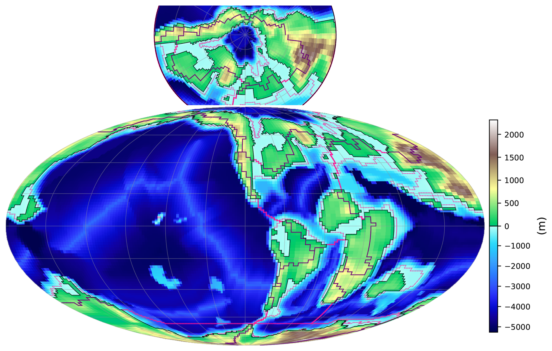
Figure 6 Map of 94 Ma paleogeography: topography (Sewall et al., 2007) and bathymetry (Müller et al., 2008) at the resolution of the climate model. Superimposed is the horizontal division of the oceanic basin in GEOCLIM (thick red lines), with the margin/open-ocean subdivision for each basin (thin red lines) and the associated continental drainage basin (purple lines). Both projections are equal-area (Mollweide and Lambert azimuthal equal-area) with identical scale.

Table 5 Values of pCO₂ and orbital parameters tested for the Turonian GCM simulations, yielding a total of 32 unique combinations.

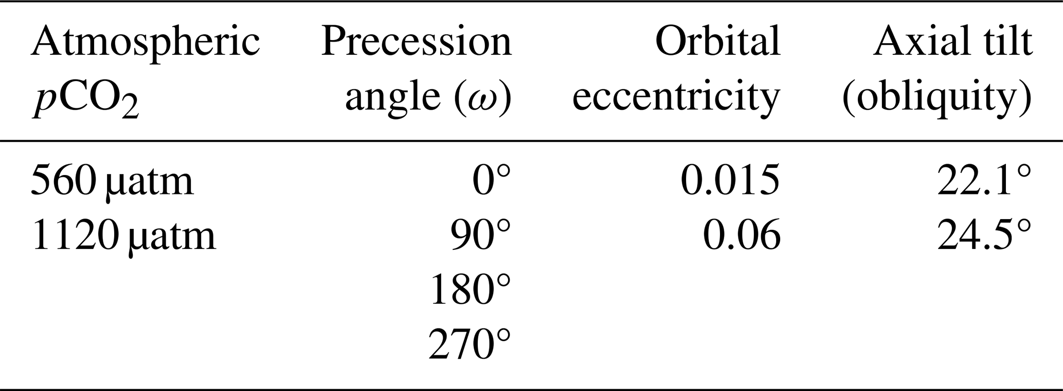
4.3 Design of GEOCLIM simulations

Several configurations of GEOCLIM oceanic boxes have been tested, as illustrated in Fig. 7. Configuration o13 is similar to the default GEOCLIM configuration, with the global open ocean divided into northern high latitudes, midlatitudes, and southern high latitudes. The “northern high latitudes” correspond to the Arctic basin, which is disconnected from the other basins except for three passages shallower than 200 m (see Fig. 6). Because of the large area occupied by shallow and epicontinental seas during the Cretaceous (much more than in modern geography) but also because we are aiming to use GEOCLIM to work on epicontinental records, the default GEOCLIM configuration with a single worldwide coastal box (separated into two vertical levels) becomes less relevant. Instead, all Turonian configurations have been defined with one coastal box (still split into two vertical levels) per oceanic basin. In the present case (o13), this makes a total of 13 oceanic boxes (seven open-ocean boxes and six coastal boxes). This default configuration, however, is not adapted to investigate the possibility of regional oceanic oxygen variations. Drawing from Laugié et al. (2021)'s results that demonstrated the proneness of the proto-Atlantic basin to become anoxic, we have designed other configurations isolating the Atlantic into a single box (configuration o22), or divided into a north and a south basin (configuration o27). Furthermore, in the Arctic basin, no deep convection occurs in the IPSL-CM5A2 experiments. Thus, it appears unrealistic to represent its surface with a 900 m deep well-mixed box, like default GEOCLIM's high-latitude boxes. An additional configuration (o28) was then made, with the Arctic basin vertically discretized in three levels, like the midlatitude basins. Another feature of GEOCLIM's default configuration becomes inconsistent with Turonian configurations: primary productivity is reduced in open-ocean polar boxes to account for the light limitation (see Eq. 24 in Sect. 2.2.4). Yet, no such reduction can be applied to the single, worldwide coastal box of GEOCLIM's default configuration. Because we design a separate coastal box for each open-ocean basin, we have applied the same reduction of Eq. (24) in all the high-latitude coastal boxes, which we refer to as configuration o28'. Last but not least, as described in Sect. 3 and Fig. 4, one also needs to define the continental drainage basins corresponding to the GEOCLIM coastal boxes. These oceanic division and drainage basins are shown in Fig. 6.

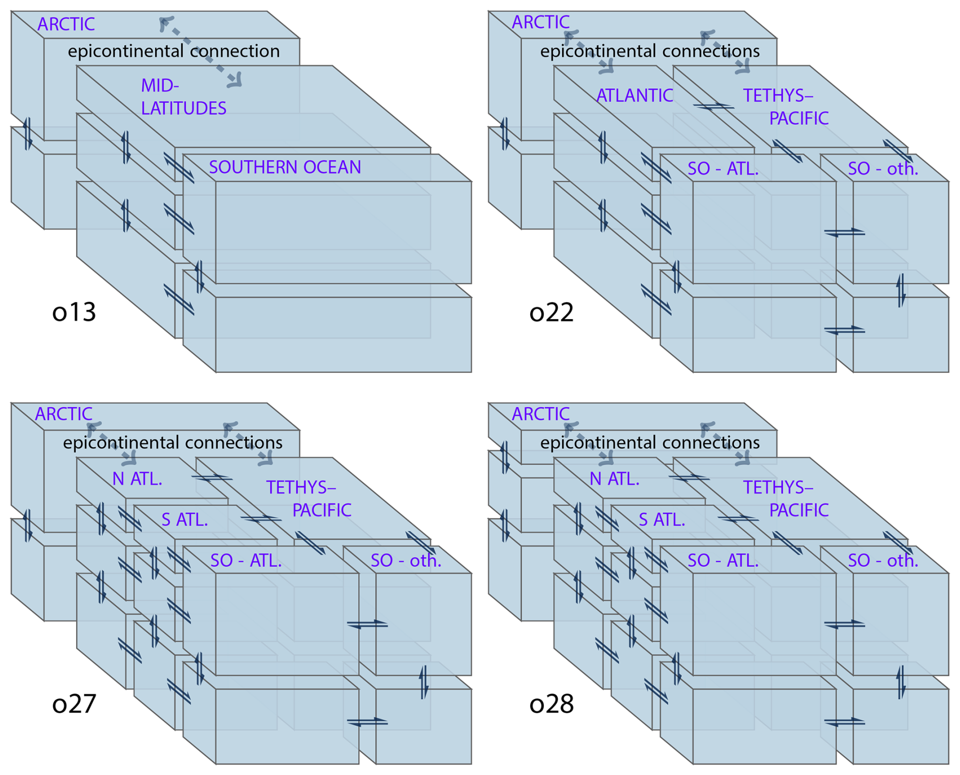
Figure 7 Schematics of the GEOCLIM ocean–ocean box discretization, showing the four main configurations tested for the Cenomanian–Turonian experiments: o13, o22, o27, and o28. Note that for each horizontal oceanic basin (i.e., each water column), there are two associated coastal ocean boxes (two vertical levels). This gives the total number of oceanic boxes: 13, 22, 27, and 28 (respectively).

Finally, guided by hints of an overestimation of the horizontal mixing between North Atlantic and Tethys–Pacific basins (discussed in the following section), we design three additional configurations with bidirectional water exchanges between the corresponding boxes reduced by 50 %, 75 %, or 100 % (configurations o28'-APx0.5, o28'-APx0.25, and o28'-APx0, respectively). The water exchanges between a box i and a box j consist of two fluxes: W_ij and W_ji. They can be split into a bidirectional flux W^B and a net flux W^N: $W_{ij}=W^{\mathrm{B}}+W_{ij}^{\mathrm{N}}$ and $W_{ji}=W^{\mathrm{B}}+W_{ji}^{\mathrm{N}}$, with $W^{\mathrm{B}}=min(W_{ij},W_{ji})$, and W^N the remaining term, only one of $W_{ij}^{\mathrm{N}}$ and $W_{ji}^{\mathrm{N}}$ being nonzero. Conceptually, W^B represents water mixing between boxes i and j, while W^N represents the unidirectional water advection. In configurations o28'-APx0.5, o28'-APx0.25, and o28'-APx0, we have recomputed W_ij and W_ji for all three vertical levels of “North Atlantic” and “Tethys–Pacific” basins by multiplying W^B by 0.5 or 0.25 or setting it to 0 (respectively), while keeping W^N unchanged. We therefore reduce the mixing of those basins without affecting the net water fluxes.

The eight configurations presented in this section are summarized in Table 6. Concerning the other boundary conditions, the degassing fluxes are set to obtain a background equilibrium pCO₂ between the two CO₂ levels of the climate experiments. The 94 Ma slope field is generated from the paleotopography reconstruction, following the method described in Sect. 3.4.1. For the lithology distribution, we use a spatially uniform lithology, keeping the global pre-industrial fractions (which is the neutral assumption mentioned in Sect. 3.4.2).

Table 6 Description of the eight tested GEOCLIM Cenomanian–Turonian configurations. The one in bold (o28'-APx0.25) was selected for the transient simulations. The first three letters of each configuration name (e.g., “o28”) correspond to the box discretization shown in Fig. 7.

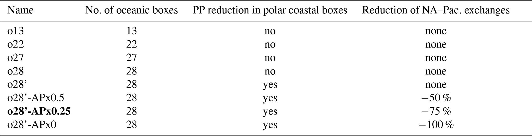
PP: primary productivity. NA: North Atlantic. Pac.: Pacific.

4.4 Steady-state oxygen distribution

We first run “equilibrium” GEOCLIM simulations for the eight configurations presented in Table 6. These simulations have been conducted at a fixed CO₂ level (560 ppm) using the averaged climate fields over all orbital configurations (i.e., the average of the 16 climate simulations at 2×CO₂) and using acceleration techniques to reach the steady state of all geochemical cycles more rapidly. These acceleration techniques were already used in Maffre et al. (2021) and consist of two parts. The first part is to multiply by a factor $\mathrm{1}/A$ the time derivatives in Eqs. (7) (atmospheric oxygen) and (8) (oceanic sulfate). The steady state achieved by the model is rigorously identical, since the time derivative is null at steady state, but the time needed to reach the steady state of the given equation is divided by A. The second part is to reduce the characteristic timescale of regolith equations (Eqs. 76–80), with the method described in Maffre (2018, Chap. 5) that reduces the time needed to reach regolith steady state while keeping this steady state rigorously identical. In the present “equilibrium” simulations, a factor A of 33 has been applied to the O and S, and the regolith characteristic timescale has been divided by 1000. With these acceleration techniques, 10 Myr of simulation is enough to reach the steady state of all GEOCLIM components. In the section, we analyze the last time step of these simulations.

Figure 8 shows the vertical profiles of open-ocean oxygen of the eight steady-state simulations. Profiles are plotted by simply taking the individual values of every oceanic box and applying them to their corresponding levels: 0–100 m, 100–900 m, and 900 m–bottom. The illustrated results indicate that having three vertical levels in the Arctic (Fig. 8d vs. 8a–c) and reducing the primary productivity in coastal polar boxes (Fig. 8e vs. 8d) are necessary to avoid unrealistic anoxic bottom Arctic water. These arbitrary choices are supported by Laugié et al. (2021), who showed more oxygenated water in the Arctic than in the Atlantic using the higher-complexity biogeochemical model PISCES embedded in the Earth system model IPSL-CM5A2. With midlatitudes divided between the Atlantic and the remaining oceans (Tethys–Pacific), and with the further division of the Atlantic into north and south, GEOCLIM does not show an oxygenation contrast exceeding ∼20 mmol m⁻³ between the (North) Atlantic and the Tethys–Pacific, although lower O₂ levels are indeed found in the Atlantic (Fig. 8b–e).

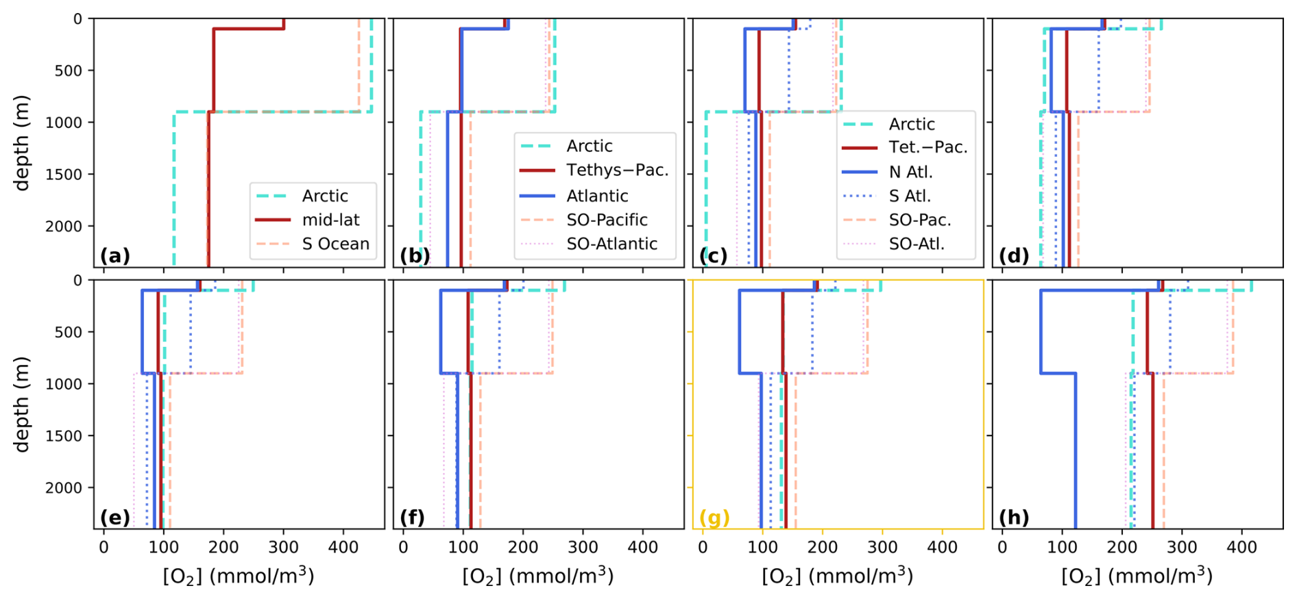
Figure 8 Vertical profiles of O₂ concentration at steady state in open-ocean GEOCLIM boxes for the eight configurations described in Table 6: (a) o13, (b) o22, (c) o27, (d) o28, (e) o28', (f) o28'-APx0.5, (g) o28'-APx0.25, and (h) o28'-APx0. The color code in panels (d–h) is the same as in (c). The configuration o28'-APx0.25 (g) was selected for transient simulations and is framed and labeled in gold. Note that though the depth is truncated, the bottom boxes extend from 900 to ∼4000 m.

In comparison, Laugié et al. (2021)'s experiments – performed with IPSL-CM5A2 and PISCES – showed an O₂ concentration difference of 100–200 mmol m⁻³ between the North Atlantic and Pacific. The analysis of the last three configurations (o28'-APx0.5, o28'-APx0.25, and o28'-APx0) in which we artificially reduce the mixing between North Atlantic boxes and Tethys–Pacific boxes (by 50 %, 75 %, and 100 %, respectively) shows promising results. The resulting O₂ profiles are shown in Fig. 8f–h. The configuration o28'-APx0.25 (Fig. 8g) appears to be the most consistent with Laugié et al. (2021). Figure 9 shows the O₂ concentration of the latter configuration on a map, where the individual values are “spread” on the entire definition area of GEOCLIM boxes (on the grid of the IPSL oceanic module). The seafloor map (Fig. 9b) also indicates that the lowest O₂ concentration (1.5 mmol m⁻³) is found in the North Atlantic coastal box below 100 m. This results from the combination of low O₂ in the surrounding open-ocean North Atlantic intermediate waters (61 mmol m⁻³) and high primary productivity due to the proximity to the coast and the large extent of the North Atlantic drainage basin (Fig. 6), conveying nutrients from continental weathering into this narrow oceanic basin.

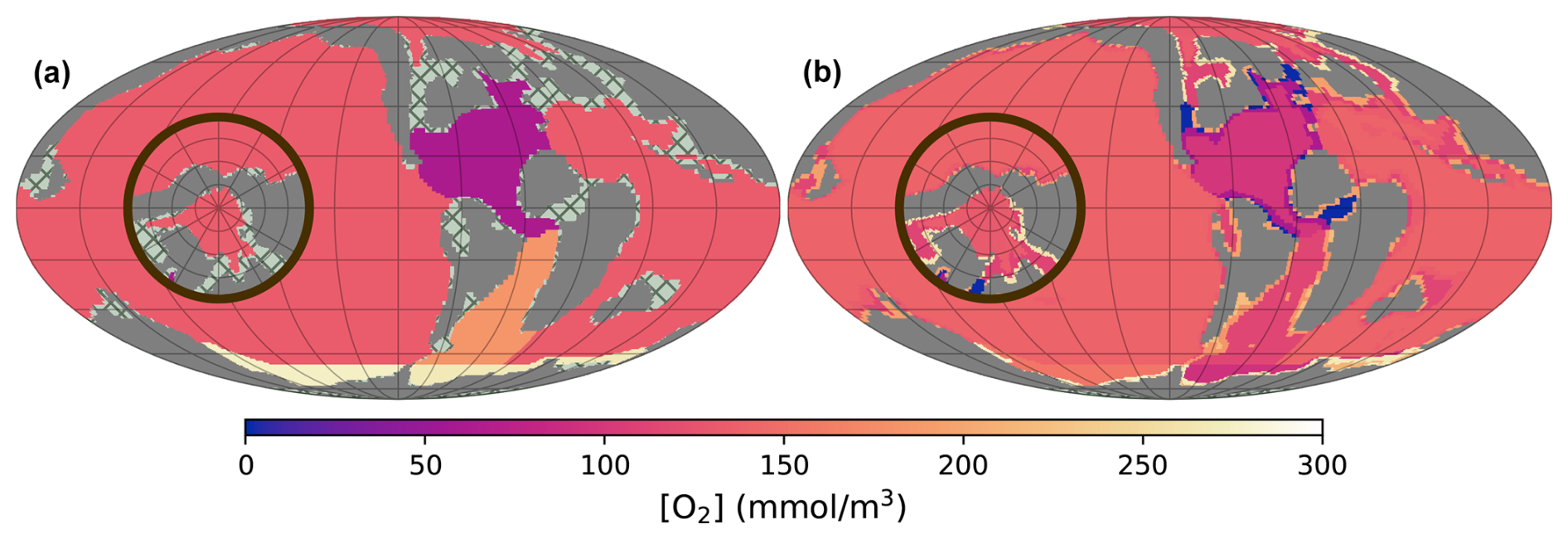
Figure 9 Oceanic O₂ concentration at an intermediate depth of 100–900 m (a) and at the bottom of the water column (b). The GEOCLIM configuration shown here is the selected one (cf. Fig. 8g) at steady state (average of all orbital configurations) and 2×CO₂. The same projections as in Fig. 6 were used; they are equal-area with identical scale.

4.5 Transient simulations: a focus on the oceanic oxygen response to orbital variations

As discussed in the “General context” section, orbital variations can influence oceanic oxygen content through various Earth system feedbacks, such as changes in continental nutrient fluxes and ocean dynamics that can modify internal nutrient distribution. Reminding the readers that the primary goal of this paper is to present the last version of GEOCLIM, this section is intended to show one potential outcome of GEOCLIM among many others. We start by describing how atmospheric CO₂ and global temperature behave in a transient simulation forced by the time series of orbital parameters using the last configuration described above (o28'-APx0.25). Thereafter, we emphasize the striking behavior of oceanic oxygen content.

All transient simulations presented here start from a steady state achieved in a similar manner as explained in Sect. 4.4, but with an imposed degassing at 5 Tmol yr⁻¹ instead of a fixed atmospheric pCO₂, as mentioned in Sect. 4.3. Climate fields evolve following the orbital parameters and following the variations of pCO₂. Figure 10 shows how pCO₂ and global mean surface temperature evolve during the first 4 Myr of simulation. The whole 10 Myr time series in not shown for the sake of readability. The pCO₂ variations driven by orbital cycles are ∼30 µatm, while the variations of global mean temperature are ∼1.25 °C. The only similar study, to our knowledge, investigating global geochemical response to orbital cycles with an Earth system model is Vervoort et al. (2024). Using the model cGENIE, with an idealized continental configuration, they found similar ranges of variation: 77 ppm for pCO₂, about twice as much as the present study, though with a higher background pCO₂ (834 ppm) and ∼1 °C of global mean temperature. Given the climate sensitivity of IPSL-CM5A2 (5.35 °C per CO₂ doubling in our 90 Ma simulations), the pCO₂ variations could only explain 0.31 °C of temperature variations. Temperature variations are then essentially a direct consequence of changes in orbital configuration. There is a tendency for cooler (warmer) temperature (±0.5 °C) at low (high) orbital eccentricity, whatever the precession value (Fig. 10a and c), which appears to be consistent with a global radiative forcing of +0.65 W m⁻² between the highest (0.15) and lowest (0.06) eccentricity value and a climate sensitivity $\stackrel{\mathrm{̃}}{\mathit{\lambda }}$ of ∼0.8 K W⁻² m². There is also a global temperature difference of $\sim +\mathrm{0.5}$ °C between the highest obliquity of 24.5° and the lowest of 22.1° (Fig. 10e and f).

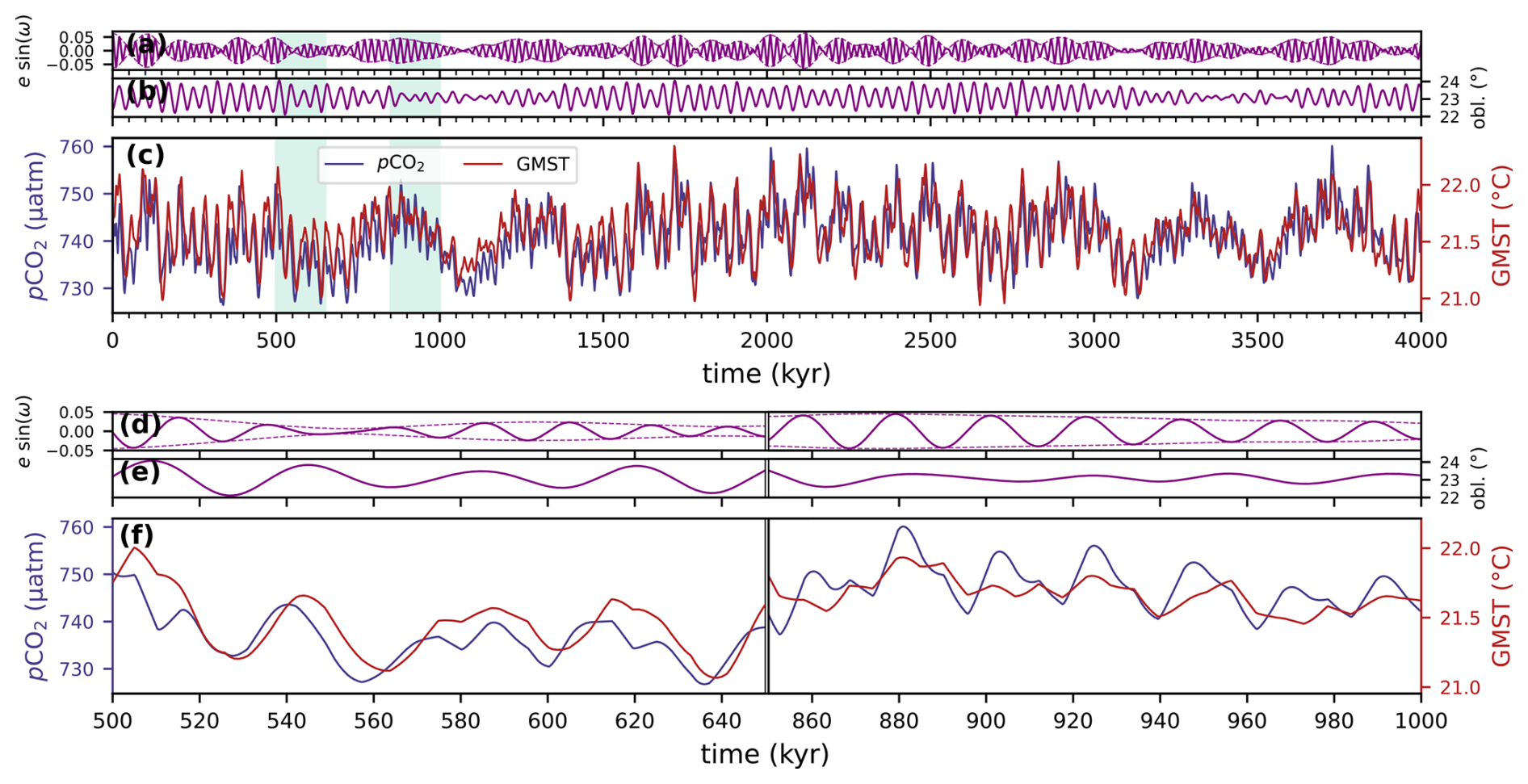
Figure 10 Time series of orbital parameters (a, b, d, f), atmospheric pCO₂, and global mean surface temperature (c, f). First 4 Myr of the 10 Myr long GEOCLIM simulation with the Laskar 95–85 Ma orbital solution, configuration o28'-APx0.25 (see Table 6), and CO₂ degassing set to 5 Tmol yr⁻¹. Panels (d)–(f) show a zoom of the two time ranges indicated by the green shading in panels (a)–(c), emphasizing the signal from obliquity (left block) and from precession (right block).

Figure 11 shows the evolution of the open-ocean oxygen concentration for two selected time ranges of the whole 10 Myr time series, highlighting the precession cycles and the obliquity cycles. The largest O₂ variations are observed in the Arctic basin at ∼100 mmol m⁻³ (Fig. 11c). The North Atlantic basin shows variations of ∼20 mmol m⁻³ (Fig. 11d), while the Tethys–Pacific basins have variations of 5–10 mmol m⁻³ (Fig. 11e and f). Arctic O₂ variations essentially respond to the precession cycle, with which they are nearly exactly in phase, with minimum O₂ during boreal summer perihelion ($e\sin \left(\mathit{\omega }\right)=-\mathrm{0.05}$, most obvious in the 850–1000 kyr time range in Fig. 11c). The prevalence of precession cycles in Arctic O₂ variations is also confirmed by a Fourier analysis of the whole 10 Myr time series (see Fig. D1 in Appendix D). In contrast, North Atlantic O₂ variations are affected by both precession and obliquity cycles, with a somewhat bigger contribution of obliquity (Fig. D1). Minimum O₂ starts during boreal spring (vernal) perihelion (e sin (ω)=0 and decreasing) and continues until the boreal summer perihelion (see the 850–1000 kyr time range in Fig. 11d). This result is consistent with Sarr et al. (2022), who used the same climate simulations but coupled with a way more complex biogeochemical model (PISCES). They found the same timing of minimum Atlantic oxygenation within the precession cycle and linked it to a diminution of the ventilation by the overturning circulation.

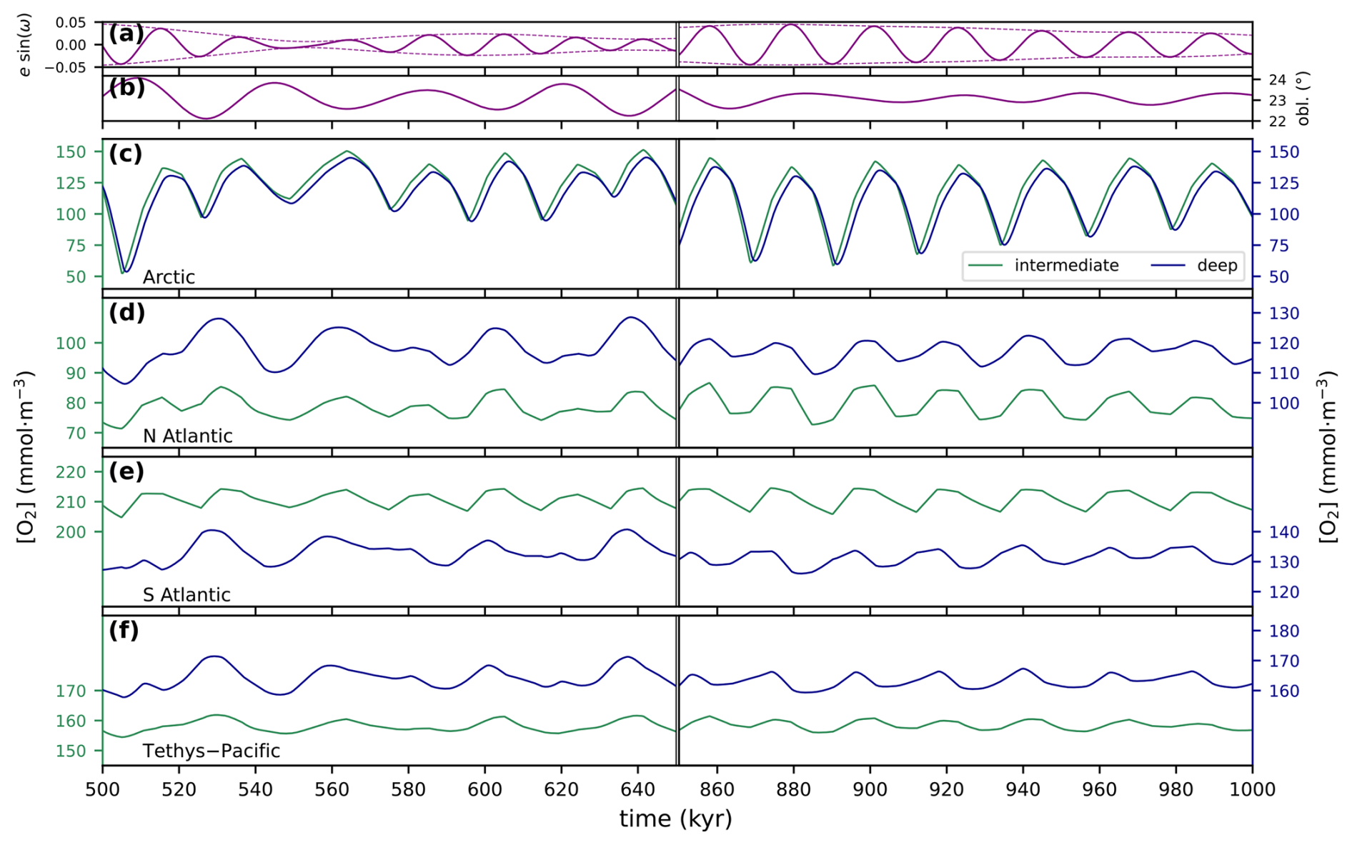
Figure 11 Orbital parameters and oxygen concentration in open-ocean GEOCLIM boxes. Transient GEOCLIM simulation with configuration o28'-APx0.25 (see Table 6). The broken time axis shows two selected time ranges of the Laskar 95–85 Ma solution, illustrating the sensitivity to the obliquity (left half) or the precession cycle (right half). (a) Eccentricity (thin dashed line) and eccentricity times the sine of the precession angle (solid line), (b) obliquity, and the (c–f) O₂ concentration in the (c) Arctic basin, (d) North Atlantic basin, (e) South Atlantic basin, and (f) Tethys–Pacific. The “y” scaling is identical in (d)–(f) for both the left and right axis, but with different offsets. Panel (c) has a different “y” scaling because of the much larger oxygen variations in the Arctic. The legend in (c) holds for (c)–(f).

The most notable feature of the GEOCLIM simulation with 95–85 Ma time series of orbital parameters is the ∼100 mmol m⁻³ variation of Arctic oxygen concentration. To determine which processes are responsible for these large oscillations, we repeat the experiment to isolate the role of continental fluxes, oceanic temperature, and oceanic circulation. Continental fluxes bring nutrients into the photic zone, which, in turn, can drive changes in primary productivity and thus more or less O₂ consumption through the oxic degradation of organic matter in the water column. Oceanic temperatures act on the solubility of oxygen and can then control the oxygen content of the deep ocean. Finally, the role of the oceanic circulation is more complex as it controls the ventilation but also the rate of primary productivity in the open ocean (which as explained above will also influence the oxygen content through oxic degradation). For each of these processes, we set the other two at a constant value from the equilibrium initial condition (representing the average of all orbital configurations). A fourth simulation was run with all three processes constant. This setup is summarized in Table 7. Figure 12 shows the Arctic O₂ concentration of these five experiments (including the original one, with all processes active) for the same two selected time ranges as in Fig. 11. It appears clearly that, except for the surface box (Fig. 12c), the variations of all O₂ concentrations at all depths are almost entirely driven by the variations of oceanic circulation. The surface oceanic O₂ concentration is different because it is imposed in the code to be at equilibrium with atmospheric pO₂, with equilibrium depending solely on temperature (Eq. A1, keeping in mind that salinity is held constant). Therefore, the O₂ concentration in surface boxes is fully driven by oceanic temperature. One may note, however, that surface O₂ variations (∼8 mmol m⁻³) are much smaller than deep ones (∼100 mmol m⁻³). The domination of the oceanic circulation in the oxygen content below the surface implies that continental weathering has no effect on primary productivity, which may appear to be a surprising result. Yet, a simple explanation resides in the fact that continental phosphorus inputs account for only ∼2 % of the oceanic primary productivity flux. Indeed, the global P weathering in the Cenomanian–Turonian simulation is 63.2 Gmol yr⁻¹; with a Redfield ratio of 117 (Table 1), this gives a potential net primary productivity flux of 7.4 Tmol yr⁻¹, while the total net primary productivity is actually 343 Tmol yr⁻¹. A similar conclusion could have already been drawn for the pre-industrial settings: with the fluxes indicated in Sect. 3.5 (29.3 Gmol yr⁻¹ for P weathering and 420 Tmol yr⁻¹ for primary productivity) and the same reasoning, P weathering might account for ∼0.8 % of the oceanic primary productivity. Consequently, a 1 % variation in oceanic circulation would have an instantaneous impact 50 to 100 times larger than a 1 % variation in continental weathering. However, our reasoning only accounts for the effect of primary productivity on deepwater oxygenation, while ventilation by oceanic circulation may also affect oxygen concentration.

Table 7 Description of the additional GEOCLIM Turonian simulations with disabled processes. All of those simulations have the same configuration (o28'-APx0.25), boundary conditions, and forcings. The “all processes” simulation is the one described in Sect. 4.5.

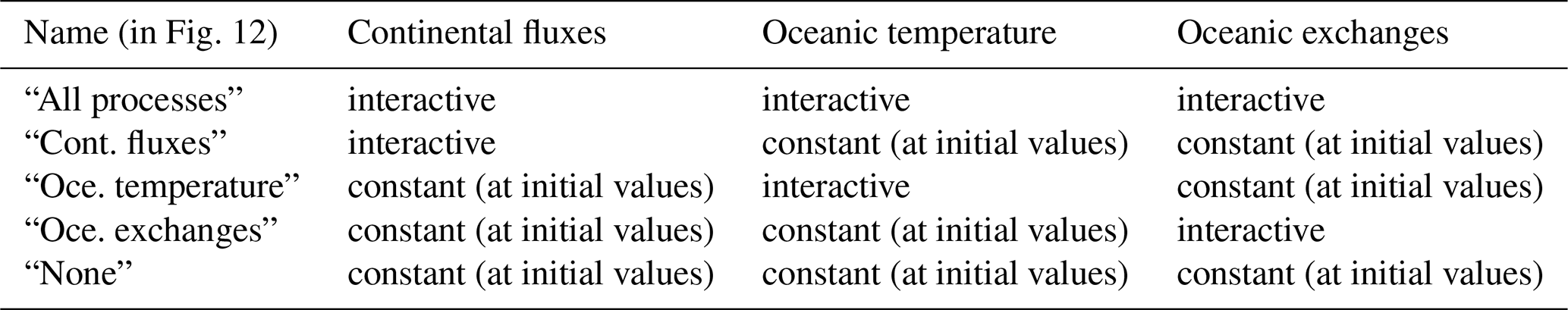
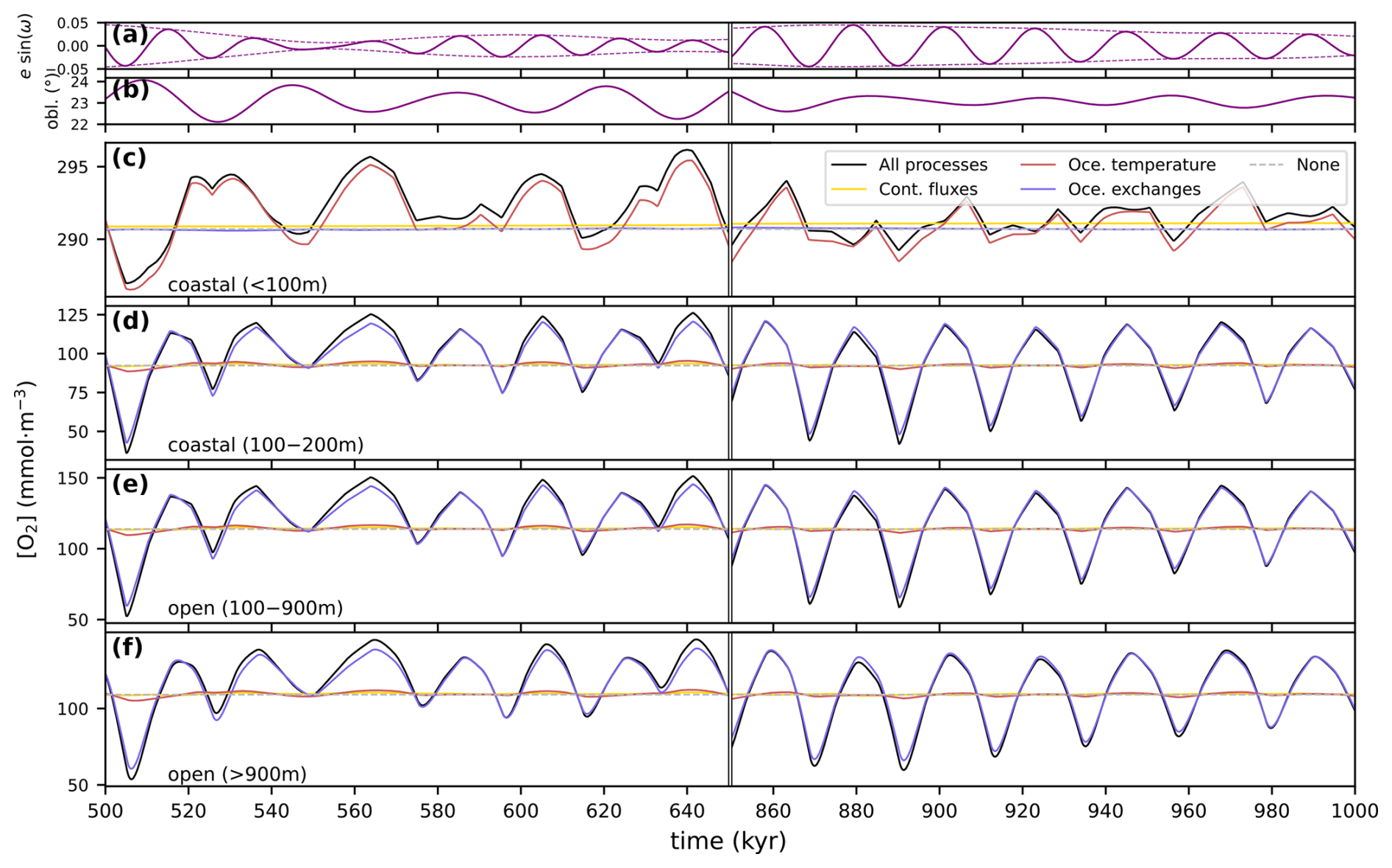
Figure 12 Orbital parameters and oxygen concentration (c–f) in the Arctic basin. Transient GEOCLIM simulation with configuration o28'-APx0.25. The same two time ranges as in Fig. 11 are shown. (a) Eccentricity (thin dashed line) and eccentricity times the sine of the precession angle (solid line), (b) obliquity, and the (c–f) O₂ concentration in the (c) coastal surface box, (d) coastal deep box, (e) open-ocean intermediate box, and (f) open-ocean deep box. Individual processes (i.e., continental fluxes, oceanic temperature, and oceanic circulation) are switched on and off. “All processes” means that all processes are “active”. In the other cases, only the mentioned process is active, and the others are kept constant at their initial values. “None” means that all the processes are kept constant.

To elucidate the exact chain of events linking variations of oceanic circulation to Arctic oxygen variations, we analyze a simulation where only oceanic circulation varies with orbital cycles (cf. Table 7) during one precession cycle, with minimum variations of obliquity (Fig. 13). The first element to note is that the oxygen variations in all non-surface Arctic boxes (Fig. 13c) are perfectly anticorrelated with the variation of the total net primary productivity in the Arctic basin (Fig. 13d), with an O₂ minimum and productivity maximum at boreal summer perihelion ($\sin \left(\mathit{\omega }\right)=-\mathrm{1}$). This observation strongly suggests productivity-driven variations of Arctic oxygenation rather than ventilation-driven. The variations of primary productivity are themselves perfectly correlated with the variations of the total P amount in the Arctic basin (Fig. 13e). The accumulation of P in the Arctic during boreal summer perihelion could a priori both be a cause or a consequence of the peak of primary productivity through the positive feedback due to more P recycling from sediment in anoxic conditions. However, the examination of net P burial flux (Fig. 13f) reveals that more P is actually buried when seawater P amount increases. This indicates that the increase in inorganic P burial, driven solely by higher P concentration (Eqs. 72 and 73), overcomes the release of P caused by deoxygenation, making the whole Arctic sedimentary system respond passively to seawater P concentration. We can therefore conclude that the accumulation of P in the Arctic is what drives the peak of primary productivity. Since this accumulation is caused by neither continental fluxes (that are set constant) nor burial fluxes, it has to be a consequence of water exchanges between the Arctic basin and the other oceans. These exchanges are investigated in Fig. 13j–q and summarized by the schematics of Fig. 14. The Arctic basin is connected to the North Atlantic by two epicontinental seaways, the Western Interior Seaway and the Fram Strait, and to the rest of the midlatitude oceans through the Western Siberian Seaway by the Tethys Ocean (Figs. 6 and 14). On the whole, Tethyan waters are entering the Arctic basin while the North Atlantic is receiving Arctic waters across the Fram Strait and the Western Interior Seaway (Figs. 13j–k and 14). When perihelion reaches boreal summer ($\sin \left(\mathit{\omega }\right)=-\mathrm{1}$), there is a subtle increase in water flux from the North Atlantic to the Arctic (from 1.00 to 1.23 Sv, Fig. 13j dashed line and Fig. 14), bringing P to the Arctic as North Atlantic waters (Fig. 13o dashed line), because of their low oxygenation, are rich in P. This effect is amplified by the decrease in water flux from the Arctic to the North Atlantic (Fig. 13j, dotted line, and Fig. 14), limiting the net P leakage (Figs. 13o and 14). The Arctic–Tethys exchanges work in the opposite way, with a decrease in water input from the Tethys (2.17 to 1.54 Sv, Fig. 13k dashed line and Fig. 14) and a slight increase in the water flux from the Arctic to the Tethys (0.04 to 0.17 Sv, Fig. 13k dotted line and Fig. 14). Yet, since Tethys waters are not particularly rich in P, these variations only lead to a moderate decrease in net P input from the Tethys (Figs. 13p and 14). In summary, when perihelion shifts from boreal winter to boreal summer, the overall amount of water flowing from the Tethys to the Arctic and exiting in the North Atlantic is reduced, increasing the water (and therefore P) residence time in Arctic. More importantly, these changes in water fluxes, though moderate (∼20 %), generate a twofold reduction of the net P leakage flux from the Arctic to the North Atlantic (Fig. 14) The resulting accumulation of P in the Arctic is responsible for the increase in primary productivity and the deoxygenation of the whole Arctic basin.

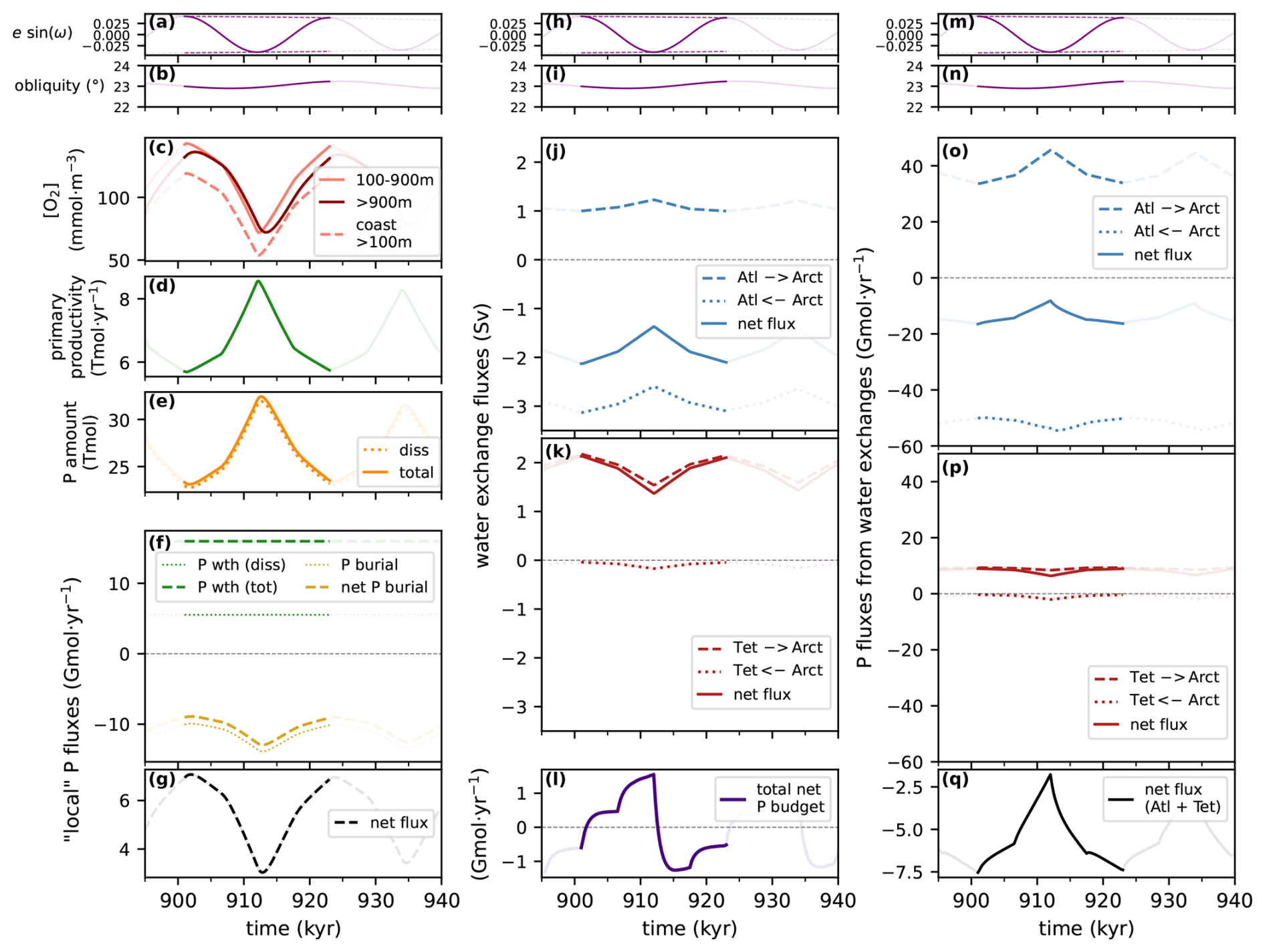
Figure 13 Orbital parameters, O₂, and budget of water and P in the whole Arctic basin. The selected time range shows a full precession cycle with minimal obliquity variation. Transient GEOCLIM simulation with configuration o28'-APx0.25 and constant continental fluxes. All water and P fluxes are positive or negative if going into or out of (respectively) the Arctic basin. In all flux panels, the value “0” is highlighted by a thin dashed horizontal line. (a, h, m) Eccentricity (thin dashed line) and eccentricity times the sine of the precession angle (solid line). (b, i, n) Obliquity. (c) O₂ concentration in non-surface boxes. (d) Net primary productivity of organic C in the whole Arctic basin. (e) P amount in the whole Arctic basin. (f) Budget of non-advective P fluxes: weathering (“wth”) and burial. The “net” P burial is the burial flux corrected from seafloor sediment leakage to other basins. The notation “diss” refers to dissolved P, while “tot” is the sum of dissolved and particulate P. (g) Budget of non-advective P fluxes, i.e., the sum of “wth tot” and “burial net” fluxes in panel (f). (j) Atlantic/Arctic water exchanges (“Atl” and “Arc”, respectively). (k) Tethys–Pacific/Arctic water exchanges (“TP” and “Arc”, respectively). (l) Total net P flux in the Arctic, i.e, the sum of panels (g) and (q); it is also the time derivative of the “total” P amount (d). (o) Atlantic–Arctic P exchanges by water advection. (p) Tethys–Pacific–Arctic P exchanges by water advection. (q) Budget of advective P fluxes, i.e., the sum of “net” fluxes in panels (o) and (p). All water and P fluxes are positive when coming into the Arctic basin and negative when going out.

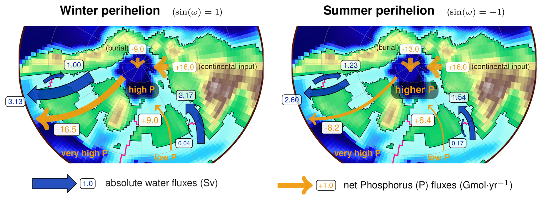
Figure 14 Schematics of the water and phosphorus budget of the Arctic at (boreal) winter and summer perihelion. Only the “net” phosphorus fluxes are indicated. These fluxes are positive (negative) when Arctic waters are gaining (losing) P. Note that the net water budget is constrained to always be null because of the non-divergence condition (see Sect. 3.2), but the P budget is not (cf. Fig. 13l).

4.6 Discussion and limitations of this study

Very few studies have attempted to investigate the response of biogeochemical cycles to orbital cycles with an Earth system model (ESM). The elements of comparison are limited to Vervoort et al. (2024), who used the intermediate-complexity model cGENIE, and Laugié et al. (2021) and Sarr et al. (2022), who used the biogeochemical model PISCES, coupled to the same climate (GCM) simulations used in the present study. The experiments of Vervoort et al. (2024) are the most similar to the ones presented here. They explored the transient evolution of geochemical cycles throughout a 3 Myr time series of orbital parameters, though with an idealized geographic configuration. However, the focus of Vervoort et al. (2024) is on the inorganic carbon cycle, preventing us from comparing our results to this pioneering study.

Sarr et al. (2022), on the other hand, investigated Cretaceous (de)oxygenation using the same 94 Ma paleogeography, but with steady-state experiments, for different orbital configurations (four cases of precession at high eccentricity and two cases of obliquity with null eccentricity) and without taking into account changes in continental weathering. Their study agrees with ours on the evolution of North Atlantic oxygenation during a precession cycle. Yet, a 28-box model has a very different representation of the world ocean than a 3D discretized model, even though the water fluxes used in GEOCLIM are derived from the same oceanic model. A model with large boxes has a tendency towards less regional contrast, as physical properties are instantaneously mixed within the boxes. This explains why GEOCLIM shows fewer regional (basin to basin) and vertical contrasts in O₂ concentration than PISCES. Such a shortcoming is inherent to box models and cannot easily be avoided. Primary productivity in GEOCLIM may also be overly sensitive to upwellings of nutrients. A stratification barrier often exists between the photic zone and deeper waters, limiting the accessibility of nutrients to the marine biosphere, even in upwelling regions. Such a barrier can only be simulated by a 3D ocean with sufficiently high resolution like PISCES. A box model like GEOCLIM is blind to it. Hence, the mechanisms driving O₂ variations in GEOCLIM may not be the same as in PISCES, even if those variations are similar. The large oscillations in Arctic O₂ concentration we observed in our GEOCLIM simulation are nonexistent in the experiments of Sarr et al. (2022). However, the restoring conditions used in PISCES should prevent transient evolution such as the one put forward in our study. Last but not least, we cannot rule out the possibility of a bias in GEOCLIM regarding polar primary productivity. Nevertheless, Arctic black shales have been identified in Earth history, notably during OAE2, possibly associated with enhanced marine bioproductivity at a latitude of around 70° N (Lenniger et al., 2014), giving some consistence to our exploratory results.

One other feature that can be learned from our simulations is the overall weak impact of variations of continental fluxes on oceanic oxygenation during orbital cycles. The main reason is that P fluxes from continental weathering only have a small contribution to oceanic primary productivity. In the Arctic basin, continental P (dissolved and particulate) accounts for ∼9 % of total P input in the coastal surface box. This input varies by ∼11 % with orbital cycles, which is consistent with the fact that the oxygen concentration varies by ∼2 % in the simulation where only continental fluxes vary (Fig. 13, yellow lines). The moderate variations (∼11 %) of continental fluxes are partly due to the fact that the Arctic has a wide drainage basin, where positive and negative anomalies and weathering rates may compensate. However, an important caveat of GEOCLIM is that continental fluxes are computed from annual mean climate variables. Although those climate variables come from a GCM that explicitly represents temporal variability, including the seasonal cycle, which determines the annual mean, the direct effect of seasonality on the computation of continental fluxes is ignored. Seasonality can be significantly more impacted by orbital parameters than the annual mean is. Yet, the impact of seasonality on weathering fluxes is disputed. Some studies (e.g., De Vleeschouwer et al., 2024; Wichern et al., 2024) have argued that stronger seasonality promotes higher weathering fluxes. But when examining concentration–discharge relationships in time series of a monitored river, a dilution behavior has often been observed (e.g., Ibarra et al., 2016, 2017) – that is, a concave runoff–weathering relationship, meaning that, for the same annual mean runoff, more seasonality would lead to a lower weathering flux. Other studies (Moquet et al., 2016) have observed a more complex relationship, with a yearly hysteresis loop, not hinting towards either an increasing or decreasing effect from seasonality.

5 Conclusions

We presented version 7 of GEOCLIM, an Earth system model suited to investigate the evolution of long-term global biogeochemical cycles and climate. The uniqueness of GEOCLIM, compared to other models aiming for similar studies, is the combination of high (GCM-like) continental resolution, intermediate oceanic resolution, high computational efficiency for multi-million-year simulations, and the coupling to a GCM at the discretion of the user, allowing directly integrating information from computationally intensive GCM simulations. This last feature offers the advantage of using physically based climate fields (land temperature and runoff, oceanic temperature and circulation) in GEOCLIM simulations, while many long-term biogeochemical cycle models have to rely on empirical parameterizations for those processes. In fact, GEOCLIM7 was conceived as an extension of a GCM, with the purpose of exploring the evolution of biogeochemical cycles based on a paleogeographic and paleoclimatic reconstruction. This characteristic was made possible by the developments presented in this article, aiming to make the oceanic discretization of GEOCLIM flexible and to derive water exchanges, seafloor sediment routing, and land water routing from any GCM simulation.

In this contribution, we have used the current version of GEOCLIM to investigate variations of oceanic oxygenation caused by orbital cycles at the beginning of the Late Cretaceous (close to OAE2). This is a pioneering modeling study as it integrates the effects of orbital parameters on oceanic and climate dynamics, geochemical fluxes (including continental erosion and weathering), and biogeochemical cycles, with an emphasis on the organic carbon cycle and oxygen. Such a study was made possible thanks to the developments published in the present article. We have found that orbital cycles can generate O₂ variations of ∼10 mmol m⁻³, up to 30 mmol m⁻³ in the proto-North Atlantic, and 100 mmol m⁻³ in the Arctic basin. We demonstrate a dominant effect of oceanic circulation in shaping the variations of oceanic O₂, with dramatically smaller magnitudes for temperature-driven and weathering-driven O₂ variations. Some of our results confirm the previous study of Sarr et al. (2022) on the sensitivity of proto-Atlantic anoxia to orbital parameters. We also identify a significantly larger sensitivity of oceanic O₂ in the Arctic ocean, though this basin stays above the dysoxic threshold in our simulation. This Arctic O₂ sensitivity to orbital cycles has not been suggested yet to our knowledge. Further work is needed on that aspect to better understand this sensitivity and obtain more constraints from data.

Appendix A: Empirical relationships for chemistry constants

This Appendix describes the empirical relationship to calculate the five chemical constants and the two isotopic equilibrium fractionation parameters used by GEOCLIM as a function of temperature, salinity, and pressure. In this entire Appendix, T is the water temperature (K), s is the salinity (PSU), and P the water pressure (atm). We remind readers that s is held constant at 35 PSU in all GEOCLIM boxes.

The solubility constant of O₂ at 1 atm, ${\mathit{\beta }}_{{\mathrm{O}}_{\mathrm{2}}}$, is expressed here in ${\mathrm{atm}}^{-\mathrm{1}}\mathrm{mol}{\mathrm{m}}^{-\mathrm{3}}$.

$$\begin{array}{}\text{(A1)}& \begin{array}{rl}& {\mathit{\beta }}_{{\mathrm{O}}_{\mathrm{2}}}=\\ & \exp \left(\begin{array}{c}-\mathrm{164.3948}+{\displaystyle \frac{\mathrm{8580.79}}{T}}+\mathrm{23.8439}\cdot \log \left(T\right)\\ +(-\mathrm{0.034892}+\mathrm{1.5568}\times {\mathrm{10}}^{-\mathrm{4}}\cdot T\\ -\mathrm{1.9387}\times {\mathrm{10}}^{-\mathrm{7}}\cdot T^{\mathrm{2}})\cdot s\end{array}\right)\end{array}\end{array}$$

The solubility constant of CO₂ at 1 atm, ${\mathit{\beta }}_{{\mathrm{CO}}_{\mathrm{2}}}$, is expressed here in ${\mathrm{atm}}^{-\mathrm{1}}\mathrm{mol}{\mathrm{m}}^{-\mathrm{3}}$.

$$\begin{array}{}\text{(A2)}& \begin{array}{rl}& {\mathit{\beta }}_{{\mathrm{CO}}_{\mathrm{2}}}=\\ & \exp \left(\begin{array}{c}-\mathrm{160.9030}+{\displaystyle \frac{\mathrm{9345.17}}{T}}+\mathrm{23.3585}\cdot \log \left(T\right)\\ +(\mathrm{0.023517}-\mathrm{2.3656}\times {\mathrm{10}}^{-\mathrm{4}}\cdot T\\ +\mathrm{4.7036}\times {\mathrm{10}}^{-\mathrm{7}}\cdot T^{\mathrm{2}})\cdot s\end{array}\right)\end{array}\end{array}$$

For both ${\mathit{\beta }}_{{\mathrm{O}}_{\mathrm{2}}}$ and ${\mathit{\beta }}_{{\mathrm{CO}}_{\mathrm{2}}}$, the pressure dependence is ignored because O₂ and CO₂ solubilities are only used at the ocean surface to compute air–sea exchanges.

The first and second acidity constants of the ${\mathrm{H}}_{\mathrm{2}}{\mathrm{CO}}_{\mathrm{3}}\rightleftharpoons {\mathrm{H}}^{+}+{\mathrm{HCO}}_{\mathrm{3}}^{-}\rightleftharpoons \mathrm{2}{\mathrm{H}}^{+}+{\mathrm{CO}}_{\mathrm{3}}^{\mathrm{2}-}$ system, K_c1 and K_c2, are both expressed in mol m⁻³.

$$\begin{array}{}\text{(A3)}& {\displaystyle }\begin{array}{rl}& K_{\text{c1}}=\\ & \exp \left(\begin{array}{c}\mathrm{297.8175}-{\displaystyle \frac{\mathrm{14}\mathrm{554.21}}{T}}-\mathrm{45.0575}\cdot \log \left(T\right)\\ +\left(\mathrm{0.0221}+{\displaystyle \frac{\mathrm{34.02}}{T}}\right)\cdot \sqrt{s}\end{array}\right)\times \\ & \exp \left({\displaystyle \frac{\left\{\begin{array}{c}(\mathrm{54.96}+\mathrm{0.151}\cdot s-\mathrm{0.1271}\cdot T)\cdot P\\ -(\mathrm{3.46}\times {\mathrm{10}}^{-\mathrm{3}}+\mathrm{2.89}\times {\mathrm{10}}^{-\mathrm{4}}\cdot s\\ -\mathrm{4.39}\times {\mathrm{10}}^{-\mathrm{5}}\cdot T)\cdot P^{\mathrm{2}}\end{array}\right\}}{\mathrm{82.056}\cdot T}}\right)\end{array}\end{array}$$

$$\begin{array}{}\text{(A4)}& {\displaystyle }\begin{array}{rl}& K_{\text{c2}}=\\ & \exp \left(\begin{array}{c}\mathrm{214.5626}-{\displaystyle \frac{\mathrm{11}\mathrm{843.79}}{T}}-\mathrm{33.6485}\cdot \log \left(T\right)\\ +\left(\mathrm{0.9805}-{\displaystyle \frac{\mathrm{92.65}}{T}}\right)\cdot \sqrt{s}-\mathrm{0.03294}\cdot s\end{array}\right)\times \\ & \exp \left({\displaystyle \frac{\left\{\begin{array}{c}(\mathrm{21.01}-\mathrm{0.321}\cdot s+\mathrm{0.0219}\cdot T)\cdot P\\ -(-\mathrm{2.617}\times {\mathrm{10}}^{-\mathrm{2}}+\mathrm{1.57}\times {\mathrm{10}}^{-\mathrm{4}}\cdot s\\ -\mathrm{7.38}\times {\mathrm{10}}^{-\mathrm{5}}\cdot T)\cdot P^{\mathrm{2}}\end{array}\right\}}{\mathrm{82.056}\cdot T}}\right)\end{array}\end{array}$$

The acidity constant of the boron system $\mathrm{B}(\mathrm{OH}{)}_{\mathrm{3}}+{\mathrm{H}}_{\mathrm{2}}\mathrm{O}\rightleftharpoons {\mathrm{H}}^{+}+\mathrm{B}(\mathrm{OH}{)}_{\mathrm{4}}^{-}$, K_b, is expressed in mol m⁻³.

$$\begin{array}{}\text{(A5)}& {\displaystyle }\begin{array}{rl}& K_{\mathrm{b}}=\\ & \exp \left(\begin{array}{c}\mathrm{154.9326}-{\displaystyle \frac{\mathrm{8966.90}}{T}}-\mathrm{24.4344}\cdot \log \left(T\right)\\ +\left(\mathrm{0.5998}-{\displaystyle \frac{\mathrm{75.25}}{T}}\right)\cdot \sqrt{s}-\mathrm{0.01767}\cdot s\end{array}\right)\times \\ & \exp \left({\displaystyle \frac{\left\{\begin{array}{c}(\mathrm{278.63}-\mathrm{0.295}\cdot s+\mathrm{1.590}\cdot T\\ +\mathrm{0.002608}\cdot T^{\mathrm{2}})\cdot P\\ -(-\mathrm{7.580}\times {\mathrm{10}}^{-\mathrm{3}}\\ +\mathrm{1.77}\times {\mathrm{10}}^{-\mathrm{4}}\cdot s)\cdot P^{\mathrm{2}}\end{array}\right\}}{\mathrm{82.056}\cdot T}}\right)\end{array}\end{array}$$

The solubility product of calcite at 1 atm, $K_{\text{sp}}^{\mathrm{o}}$, is expressed in mol² m⁻⁶.

$$\begin{array}{}\text{(A6)}& \begin{array}{rl}& K_{\text{sp}}^{\mathrm{o}}=\\ & \exp \left(\begin{array}{c}\mathrm{316.9463}-{\displaystyle \frac{\mathrm{13}\mathrm{348.09}}{T}}-\mathrm{48.7537}\cdot \log \left(T\right)\\ +\left(\mathrm{1.6233}-{\displaystyle \frac{\mathrm{118.64}}{T}}\right)\cdot \sqrt{s}-\mathrm{0.06999}\cdot s\end{array}\right)\end{array}\end{array}$$

The isotopic equilibrium fractionation parameters of ${\mathrm{H}}_{\mathrm{2}}{\mathrm{CO}}_{\mathrm{3}}\rightleftharpoons {\mathrm{H}}^{+}+{\mathrm{HCO}}_{\mathrm{3}}^{-}\rightleftharpoons \mathrm{2}{\mathrm{H}}^{+}+{\mathrm{CO}}_{\mathrm{3}}^{\mathrm{2}-}$, ϵ_D1 and ϵ_D2 (both expressed in ‰), are as follows.

$$\begin{array}{}\text{(A7)}& {\displaystyle }{\mathit{ϵ}}_{\text{D1}}& {\displaystyle }=\mathrm{24.12}-{\displaystyle \frac{\mathrm{9866}}{T}}\text{(A8)}& {\displaystyle }{\mathit{ϵ}}_{\text{D2}}& {\displaystyle }=\mathrm{0.22}+{\displaystyle \frac{\mathrm{653.627}}{(T-\mathrm{233.45}{)}^{\mathrm{2}}}}\end{array}$$

Appendix B: Resolution of the non-divergence correction optimization problem

In this section, we present the mathematical derivation of the flux matrix correction. $\stackrel{\mathrm{̃}}{\mathbf{W}}$ is the initial flux matrix, with $\stackrel{\mathrm{̃}}{\mathbf{W}}\ge \mathrm{0}$ and ${\stackrel{\mathrm{̃}}{W}}_{ii}=\mathrm{0}\forall i$. We need to transform $\stackrel{\mathrm{̃}}{\mathbf{W}}$, in the most parsimonious way, into a matrix W that satisfies the non-divergence criterion: ${\sum }_k(W_{ik}-W_{ki})=\mathrm{0}\forall i$.

B1 Additive correction

The additive correction approach defines $\mathbf{W}=\stackrel{\mathrm{̃}}{\mathbf{W}}+\mathit{\delta }$, with a least-square condition.

$$\begin{array}{}\text{(B1)}& {\displaystyle }\begin{array}{rl}\sum _j(W_{ij}-W_{ji})& =\sum _j({\stackrel{\mathrm{̃}}{W}}_{ij}+{\mathit{\delta }}_{ij}-{\stackrel{\mathrm{̃}}{W}}_{ji}-{\mathit{\delta }}_{ji})\\ & =\mathrm{0}\forall i\end{array}\text{(B2)}& {\displaystyle }\sum _i\sum _j{{\mathit{\delta }}_{ij}}^{\mathrm{2}}\text{ is minimum}\end{array}$$

Equations (B1)–(B2) are therefore a constrained optimization problem that is solved by the Lagrange multiplier method. We start by defining the divergence vector y.

$$\begin{array}{}\text{(B3)}& y_i=\sum _j({\stackrel{\mathrm{̃}}{W}}_{ij}-{\stackrel{\mathrm{̃}}{W}}_{ji})\end{array}$$

Equation (B1) can be rewritten as follows.

$$\begin{array}{}\text{(B4)}& \sum _j\left({\mathit{\delta }}_{ij}-{\mathit{\delta }}_{ji}\right)+y_i=\mathrm{0}\forall i\end{array}$$

The Lagrange multiplier method consists of incorporating both conditions in Eqs. (B2) and (B4) into a single function.

$$\begin{array}{}\text{(B5)}& \begin{array}{rl}\mathrm{\Psi }(& {\mathit{\delta }}_{\mathrm{00}},\mathrm{\dots },{\mathit{\delta }}_{ij},\mathrm{\dots },{\mathit{\delta }}_{nn},{\mathit{\lambda }}_{\mathrm{0}},\mathrm{\dots },{\mathit{\lambda }}_k,\mathrm{\dots },{\mathit{\lambda }}_n)=\\ & \sum _{i=\mathrm{1}}^n\sum _{j=\mathrm{1}}^n{{\mathit{\delta }}_{ij}}^{\mathrm{2}}+\sum _{k=\mathrm{1}}^n\left[{\mathit{\lambda }}_k\left(\sum _{j=\mathrm{1}}^n\left({\mathit{\delta }}_{kj}-{\mathit{\delta }}_{jk}\right)+y_k\right)\right]\end{array}\end{array}$$

Here, n is the number of GEOCLIM oceanic boxes (i.e., excluding the atmospheric box). Ψ is then a function of n²+n variables. The conditions in Eqs. (B2) and (B4) imply that the n²+n partial derivatives of Ψ are null.

$$\begin{array}{}\text{(B6)}& {\displaystyle \frac{\partial \mathrm{\Psi }}{\partial {\mathit{\lambda }}_{k_{\mathrm{o}}}}}=\sum _{j=\mathrm{1}}^n\left({\mathit{\delta }}_{k_{\mathrm{o}}j}-{\mathit{\delta }}_{j{k}_{\mathrm{o}}}\right)+y_{k_{\mathrm{o}}}=\mathrm{0}\end{array}$$

$$\begin{array}{}\text{(B7)}& {\displaystyle \frac{\partial \mathrm{\Psi }}{\partial {\mathit{\delta }}_{i_{\mathrm{o}}{j}_{\mathrm{o}}}}}=\mathrm{2}{\mathit{\delta }}_{i_{\mathrm{o}}{j}_{\mathrm{o}}}+{\mathit{\lambda }}_{i_{\mathrm{o}}}-{\mathit{\lambda }}_{j_{\mathrm{o}}}=\mathrm{0}\end{array}$$

Equation (B7) gives

$$\begin{array}{}\text{(B8)}& {\mathit{\delta }}_{ij}={\displaystyle \frac{{\mathit{\lambda }}_j-{\mathit{\lambda }}_i}{\mathrm{2}}}.\end{array}$$

And by substitution in Eq. (B6), the following holds.

$$\begin{array}{ll}{\displaystyle }& {\displaystyle }\sum _{j=\mathrm{1}}^n\left({\mathit{\delta }}_{ij}-{\mathit{\delta }}_{ji}\right)=-y_i\\ {\displaystyle }<=>& {\displaystyle }\sum _{j=\mathrm{1}}^n\left({\displaystyle \frac{{\mathit{\lambda }}_j-{\mathit{\lambda }}_i}{\mathrm{2}}}-{\displaystyle \frac{{\mathit{\lambda }}_i-{\mathit{\lambda }}_j}{\mathrm{2}}}\right)=-y_i\\ {\displaystyle }<=>& {\displaystyle }\sum _{j=\mathrm{1}}^n\left({\mathit{\lambda }}_j-{\mathit{\lambda }}_i\right)=-y_i\\ \text{(B9)}& {\displaystyle }<=>& {\displaystyle }n{\mathit{\lambda }}_i-\sum _{j=\mathrm{1}}^n{\mathit{\lambda }}_j=y_i\end{array}$$

Here, one must notice that the system of n equations (B9) only has n−1 linearly independent equations, and if the vector λ is a solution of Eq. (B9), then λ+c (for any constant c) is also a solution. However, this does not alter the unicity of the solution for matrix δ: given Eq. (B8), adding a constant c to λ does not change the definition of δ. We can therefore impose ${\sum }_j{\mathit{\lambda }}_j=\mathrm{0}$. One may also notice that the equation system (B9) only has a solution if ${\sum }_i{y}_i=\mathrm{0}$, which is the case. Given Eq. (B3),

$$\begin{array}{}\text{(B10)}& \begin{array}{rl}\sum _i{y}_i& =\sum _i\sum _j({\stackrel{\mathrm{̃}}{W}}_{ij}-{\stackrel{\mathrm{̃}}{W}}_{ji})\\ & =\sum _i\sum _j{\stackrel{\mathrm{̃}}{W}}_{ij}-\sum _i\sum _j{\stackrel{\mathrm{̃}}{W}}_{ji}=\mathrm{0}.\end{array}\end{array}$$

Thus, imposing ${\sum }_j{\mathit{\lambda }}_j=\mathrm{0}$, Eq. (B9) gives

$$\begin{array}{}\text{(B11)}& {\mathit{\lambda }}_i={\displaystyle \frac{y_i}{n}}.\end{array}$$

Finally, with Eq. (B8), the solution for the additive correction δ is

$$\begin{array}{}\text{(B12)}& {\mathit{\delta }}_{ij}={\displaystyle \frac{y_j-y_i}{\mathrm{2}n}}.\end{array}$$

B2 Multiplicative correction

The multiplicative correction approach defines W by $W_{ij}={\mathit{\varphi }}_{ij}{\stackrel{\mathrm{̃}}{W}}_{ij}$, with a least-square condition.

$$\begin{array}{}\text{(B13)}& {\displaystyle }& {\displaystyle }\sum _j(W_{ij}-W_{ji})=\sum _j({\mathit{\varphi }}_{ij}{\stackrel{\mathrm{̃}}{W}}_{ij}-{\mathit{\varphi }}_{ji}{\stackrel{\mathrm{̃}}{W}}_{ji})=\mathrm{0}\forall i\text{(B14)}& {\displaystyle }& {\displaystyle }\sum _i\sum _j(\mathrm{1}-{\mathit{\varphi }}_{ij}{)}^{\mathrm{2}}\text{ is minimum}\end{array}$$

The constrained optimization problem of Eqs. (B13) and (B14) is solved by the Lagrange multiplier method.

$$\begin{array}{}\text{(B15)}& \begin{array}{rl}\mathrm{\Psi }& ({\mathit{\varphi }}_{\mathrm{00}},\mathrm{\dots },{\mathit{\varphi }}_{ij},\mathrm{\dots },{\mathit{\varphi }}_{nn},{\mathit{\lambda }}_{\mathrm{0}},\mathrm{\dots },{\mathit{\lambda }}_k,\mathrm{\dots },{\mathit{\lambda }}_n)=\\ & \sum _{i=\mathrm{1}}^n\sum _{j=\mathrm{1}}^n(\mathrm{1}-{\mathit{\varphi }}_{ij}{)}^{\mathrm{2}}\\ & +\sum _{k=\mathrm{1}}^n\left[{\mathit{\lambda }}_k\left(\sum _{j=\mathrm{1}}^n\left({\mathit{\varphi }}_{kj}{\stackrel{\mathrm{̃}}{W}}_{kj}-{\mathit{\varphi }}_{jk}{\stackrel{\mathrm{̃}}{W}}_{jk}\right)\right)\right]\end{array}\end{array}$$

The n²+n partial derivatives of Ψ are set to zero.

$$\begin{array}{}\text{(B16)}& {\displaystyle \frac{\partial \mathrm{\Psi }}{\partial {\mathit{\lambda }}_{k_{\mathrm{o}}}}}=\sum _{j=\mathrm{1}}^n({\mathit{\varphi }}_{k_{\mathrm{o}}j}{\stackrel{\mathrm{̃}}{W}}_{k_{\mathrm{o}}j}-{\mathit{\varphi }}_{j{k}_{\mathrm{o}}}{\stackrel{\mathrm{̃}}{W}}_{j{k}_{\mathrm{o}}})=\mathrm{0}\end{array}$$

$$\begin{array}{}\text{(B17)}& {\displaystyle \frac{\partial \mathrm{\Psi }}{\partial {\mathit{\varphi }}_{i_{\mathrm{o}}{j}_{\mathrm{o}}}}}=-\mathrm{2}(\mathrm{1}-{\mathit{\varphi }}_{i_{\mathrm{o}}{j}_{\mathrm{o}}})+{\mathit{\lambda }}_{i_{\mathrm{o}}}{\stackrel{\mathrm{̃}}{W}}_{i_{\mathrm{o}}{j}_{\mathrm{o}}}-{\mathit{\lambda }}_{j_{\mathrm{o}}}{\stackrel{\mathrm{̃}}{W}}_{i_{\mathrm{o}}{j}_{\mathrm{o}}}=\mathrm{0}\end{array}$$

Equation (B17) gives the following.

$$\begin{array}{}\text{(B18)}& {\mathit{\varphi }}_{ij}=\mathrm{1}-{\displaystyle \frac{{\mathit{\lambda }}_i{\stackrel{\mathrm{̃}}{W}}_{ij}-{\mathit{\lambda }}_j{\stackrel{\mathrm{̃}}{W}}_{ij}}{\mathrm{2}}}=\mathrm{1}+{\displaystyle \frac{{\mathit{\lambda }}_j-{\mathit{\lambda }}_i}{\mathrm{2}}}{\stackrel{\mathrm{̃}}{W}}_{ij}\end{array}$$

By substitution in Eq. (B16), the following holds.

$$\begin{array}{ll}{\displaystyle }\sum _{j=\mathrm{1}}^n(& {\displaystyle }{\mathit{\varphi }}_{ij}{\stackrel{\mathrm{̃}}{W}}_{ij}-{\mathit{\varphi }}_{ji}{\stackrel{\mathrm{̃}}{W}}_{ji})=\mathrm{0}\\ {\displaystyle }<=>\sum _{j=\mathrm{1}}^n[& {\displaystyle }(\mathrm{1}+{\displaystyle \frac{{\mathit{\lambda }}_j-{\mathit{\lambda }}_i}{\mathrm{2}}}{\stackrel{\mathrm{̃}}{W}}_{ij}){\stackrel{\mathrm{̃}}{W}}_{ij}\\ {\displaystyle }& {\displaystyle }-(\mathrm{1}+{\displaystyle \frac{{\mathit{\lambda }}_i-{\mathit{\lambda }}_j}{\mathrm{2}}}{\stackrel{\mathrm{̃}}{W}}_{ji}){\stackrel{\mathrm{̃}}{W}}_{ji}]=\mathrm{0}\\ {\displaystyle }<=>\sum _{j=\mathrm{1}}^n[& {\displaystyle \frac{{\mathit{\lambda }}_j-{\mathit{\lambda }}_i}{\mathrm{2}}}{\stackrel{\mathrm{̃}}{W}}_{ij}^{\mathrm{2}}-{\displaystyle \frac{{\mathit{\lambda }}_i-{\mathit{\lambda }}_j}{\mathrm{2}}}{\stackrel{\mathrm{̃}}{W}}_{ji}^{\mathrm{2}}+{\stackrel{\mathrm{̃}}{W}}_{ij}-{\stackrel{\mathrm{̃}}{W}}_{ji}]=\mathrm{0}\\ {\displaystyle }<=>\sum _{j=\mathrm{1}}^n[& {\displaystyle }{\mathit{\lambda }}_j{\displaystyle \frac{{\stackrel{\mathrm{̃}}{W}}_{ij}^{\mathrm{2}}+{\stackrel{\mathrm{̃}}{W}}_{ji}^{\mathrm{2}}}{\mathrm{2}}}-{\mathit{\lambda }}_i{\displaystyle \frac{{\stackrel{\mathrm{̃}}{W}}_{ij}^{\mathrm{2}}+{\stackrel{\mathrm{̃}}{W}}_{ji}^{\mathrm{2}}}{\mathrm{2}}}+{\stackrel{\mathrm{̃}}{W}}_{ij}-{\stackrel{\mathrm{̃}}{W}}_{ji}]=\mathrm{0}\\ {\displaystyle }<=>\sum _{j=\mathrm{1}}^n[& {\displaystyle }({\mathit{\lambda }}_j-{\mathit{\lambda }}_i){\displaystyle \frac{{\stackrel{\mathrm{̃}}{W}}_{ij}^{\mathrm{2}}+{\stackrel{\mathrm{̃}}{W}}_{ji}^{\mathrm{2}}}{\mathrm{2}}}+{\stackrel{\mathrm{̃}}{W}}_{ij}-{\stackrel{\mathrm{̃}}{W}}_{ji}]=\mathrm{0}\\ \text{(B19)}& {\displaystyle }<=>\sum _{j=\mathrm{1}}^n[& {\displaystyle }({\mathit{\lambda }}_j-{\mathit{\lambda }}_i){\displaystyle \frac{{\stackrel{\mathrm{̃}}{W}}_{ij}^{\mathrm{2}}+{\stackrel{\mathrm{̃}}{W}}_{ji}^{\mathrm{2}}}{\mathrm{2}}}]=-y_i\end{array}$$

With the same definition of the divergence vector y as in Sect. B1,

$$\begin{array}{}\text{(B20)}& y_i=\sum _j({\stackrel{\mathrm{̃}}{W}}_{ij}-{\stackrel{\mathrm{̃}}{W}}_{ji}).\end{array}$$

Here again, one must notice that the system of equations (B19) only has, at most, n−1 linearly independent equations: applying ∑_i to Eq. (B19) gives the following.

$$\begin{array}{ll}{\displaystyle }& {\displaystyle }\sum _{i=\mathrm{1}}^n\sum _{j=\mathrm{1}}^n\left({\mathit{\lambda }}_j-{\mathit{\lambda }}_i\right){\displaystyle \frac{{\stackrel{\mathrm{̃}}{W}}_{ij}^{\mathrm{2}}+{\stackrel{\mathrm{̃}}{W}}_{ji}^{\mathrm{2}}}{\mathrm{2}}}=-\sum _{i=\mathrm{1}}^n{y}_i\\ {\displaystyle }<=>& {\displaystyle }\sum _{i=\mathrm{1}}^n\sum _{j=\mathrm{1}}^n{\mathit{\lambda }}_j{\displaystyle \frac{{\stackrel{\mathrm{̃}}{W}}_{ij}^{\mathrm{2}}+{\stackrel{\mathrm{̃}}{W}}_{ji}^{\mathrm{2}}}{\mathrm{2}}}\\ {\displaystyle }& {\displaystyle }-\sum _{i=\mathrm{1}}^n\sum _{j=\mathrm{1}}^n{\mathit{\lambda }}_i{\displaystyle \frac{{\stackrel{\mathrm{̃}}{W}}_{ij}^{\mathrm{2}}+{\stackrel{\mathrm{̃}}{W}}_{ji}^{\mathrm{2}}}{\mathrm{2}}}=-\sum _{i=\mathrm{1}}^n{y}_i\\ {\displaystyle }<=>& {\displaystyle }\sum _{i=\mathrm{1}}^n\sum _{j=\mathrm{1}}^n{\mathit{\lambda }}_j{\displaystyle \frac{{\stackrel{\mathrm{̃}}{W}}_{ij}^{\mathrm{2}}+{\stackrel{\mathrm{̃}}{W}}_{ji}^{\mathrm{2}}}{\mathrm{2}}}\\ {\displaystyle }& {\displaystyle }-\sum _{j=\mathrm{1}}^n\sum _{i=\mathrm{1}}^n{\mathit{\lambda }}_i{\displaystyle \frac{{\stackrel{\mathrm{̃}}{W}}_{ji}^{\mathrm{2}}+{\stackrel{\mathrm{̃}}{W}}_{ij}^{\mathrm{2}}}{\mathrm{2}}}=-\sum _{i=\mathrm{1}}^n{y}_i\\ \text{(B21)}& {\displaystyle }<=>& {\displaystyle }\mathrm{0}=-\sum _{i=\mathrm{1}}^n{y}_i\end{array}$$

And we show in Appendix B1 that we indeed have ${\sum }_i{y}_i=\mathrm{0}$. In addition, one may notice that, as in Appendix B1, if λ is a solution of Eq. (B19), then λ+c (for any constant c) is also a solution and that adding c does not change the value of ϕ (Eq. B18). We therefore choose to impose ${\sum }_i{\mathit{\lambda }}_i=\mathrm{0}$. To do so, we use the following change of variables to substitute vector λ by vector x.

$$\begin{array}{}\text{(B22)}& \left\{\begin{array}{rl}{\displaystyle }{x}_{\mathrm{1}}& {\displaystyle }={\mathit{\lambda }}_{\mathrm{1}}\\ {\displaystyle }{x}_{\mathrm{2}}& {\displaystyle }={\mathit{\lambda }}_{\mathrm{2}}\\ {\displaystyle }& {\displaystyle }\mathrm{\dots }\\ {\displaystyle }{x}_n& {\displaystyle }={\sum }_{k=\mathrm{1}}^n{\mathit{\lambda }}_k\end{array}\right.<=>\left\{\begin{array}{rl}{\displaystyle }{\mathit{\lambda }}_{\mathrm{1}}& {\displaystyle }=x_{\mathrm{1}}\\ {\displaystyle }{\mathit{\lambda }}_{\mathrm{2}}& {\displaystyle }=x_{\mathrm{2}}\\ {\displaystyle }& {\displaystyle }\mathrm{\dots }\\ {\displaystyle }{\mathit{\lambda }}_n& {\displaystyle }=x_n-{\sum }_{k=\mathrm{1}}^{n-\mathrm{1}}{x}_k\end{array}\right.\end{array}$$

Equation (B19) is only solved for i≠n and i=n. Indeed, the last equation (i=n) can be deduced from the first n−1 ones. Hence, $\forall i\ne n$.

$$\begin{array}{ll}{\displaystyle }& {\displaystyle }\sum _{j=\mathrm{1}}^n\left[\left({\mathit{\lambda }}_j-{\mathit{\lambda }}_i\right){\displaystyle \frac{{\stackrel{\mathrm{̃}}{W}}_{ij}^{\mathrm{2}}+{\stackrel{\mathrm{̃}}{W}}_{ji}^{\mathrm{2}}}{\mathrm{2}}}\right]=-y_i\\ {\displaystyle }<=>& {\displaystyle }\sum _{j=\mathrm{1}}^{n-\mathrm{1}}\left[\left(x_j-x_i\right){\displaystyle \frac{{\stackrel{\mathrm{̃}}{W}}_{ij}^{\mathrm{2}}+{\stackrel{\mathrm{̃}}{W}}_{ji}^{\mathrm{2}}}{\mathrm{2}}}\right]\\ {\displaystyle }& {\displaystyle }+\left[\left(x_n-\sum _{k=\mathrm{1}}^{n-\mathrm{1}}{x}_k-x_i\right){\displaystyle \frac{{\stackrel{\mathrm{̃}}{W}}_{in}^{\mathrm{2}}+{\stackrel{\mathrm{̃}}{W}}_{ni}^{\mathrm{2}}}{\mathrm{2}}}\right]=-y_i\end{array}$$

Using the fact that x_n=0 (corollary of ${\sum }_i{\mathit{\lambda }}_i=\mathrm{0}$), the following holds.

$$\begin{array}{ll}{\displaystyle }<=>& {\displaystyle }\sum _{j=\mathrm{1}}^{n-\mathrm{1}}{x}_j{\displaystyle \frac{{\stackrel{\mathrm{̃}}{W}}_{ij}^{\mathrm{2}}+{\stackrel{\mathrm{̃}}{W}}_{ji}^{\mathrm{2}}}{\mathrm{2}}}-\sum _{j=\mathrm{1}}^{n-\mathrm{1}}{x}_i{\displaystyle \frac{{\stackrel{\mathrm{̃}}{W}}_{ij}^{\mathrm{2}}+{\stackrel{\mathrm{̃}}{W}}_{ji}^{\mathrm{2}}}{\mathrm{2}}}\\ {\displaystyle }& {\displaystyle }-\left(\sum _{k=\mathrm{1}}^{n-\mathrm{1}}{x}_k\right){\displaystyle \frac{{\stackrel{\mathrm{̃}}{W}}_{in}^{\mathrm{2}}+{\stackrel{\mathrm{̃}}{W}}_{ni}^{\mathrm{2}}}{\mathrm{2}}}-x_i{\displaystyle \frac{{\stackrel{\mathrm{̃}}{W}}_{in}^{\mathrm{2}}+{\stackrel{\mathrm{̃}}{W}}_{ni}^{\mathrm{2}}}{\mathrm{2}}}=-y_i\\ {\displaystyle }<=>& {\displaystyle }\sum _{j=\mathrm{1}}^{n-\mathrm{1}}{x}_j{\displaystyle \frac{{\stackrel{\mathrm{̃}}{W}}_{ij}^{\mathrm{2}}+{\stackrel{\mathrm{̃}}{W}}_{ji}^{\mathrm{2}}}{\mathrm{2}}}-\sum _{k=\mathrm{1}}^{n-\mathrm{1}}{x}_k{\displaystyle \frac{{\stackrel{\mathrm{̃}}{W}}_{in}^{\mathrm{2}}+{\stackrel{\mathrm{̃}}{W}}_{ni}^{\mathrm{2}}}{\mathrm{2}}}\\ {\displaystyle }& {\displaystyle }-\sum _{j=\mathrm{1}}^n{x}_i{\displaystyle \frac{{\stackrel{\mathrm{̃}}{W}}_{ij}^{\mathrm{2}}+{\stackrel{\mathrm{̃}}{W}}_{ji}^{\mathrm{2}}}{\mathrm{2}}}=-y_i\end{array}$$

Then, substituting k for i in the sum of the second term gives the following.

$$\begin{array}{}\text{(B23)}& \begin{array}{rl}<=>& \sum _{j=\mathrm{1}}^{n-\mathrm{1}}{\displaystyle \frac{{\stackrel{\mathrm{̃}}{W}}_{in}^{\mathrm{2}}+{\stackrel{\mathrm{̃}}{W}}_{ni}^{\mathrm{2}}-{\stackrel{\mathrm{̃}}{W}}_{ij}^{\mathrm{2}}-{\stackrel{\mathrm{̃}}{W}}_{ji}^{\mathrm{2}}}{\mathrm{2}}}{x}_j\\ & +\left(\sum _{j=\mathrm{1}}^n{\displaystyle \frac{{\stackrel{\mathrm{̃}}{W}}_{ij}^{\mathrm{2}}+{\stackrel{\mathrm{̃}}{W}}_{ji}^{\mathrm{2}}}{\mathrm{2}}}\right)x_i=y_i\end{array}\end{array}$$

Equation (B23) is a linear system $\mathbf{M}\cdot \mathit{x}=\mathit{y}$ (of n−1 equations and n−1 unknown x_i), with M a size (n−1) square matrix defined by

$$\begin{array}{}\text{(B24)}& M_{ij}=\left\{\begin{array}{ll}\frac{\mathrm{1}}{\mathrm{2}}({\stackrel{\mathrm{̃}}{W}}_{in}^{\mathrm{2}}+{\stackrel{\mathrm{̃}}{W}}_{ni}^{\mathrm{2}}-{\stackrel{\mathrm{̃}}{W}}_{ij}^{\mathrm{2}}-{\stackrel{\mathrm{̃}}{W}}_{ji}^{\mathrm{2}})& \text{if}i\ne j\\ \frac{\mathrm{1}}{\mathrm{2}}({\stackrel{\mathrm{̃}}{W}}_{in}^{\mathrm{2}}+{\stackrel{\mathrm{̃}}{W}}_{ni}^{\mathrm{2}}-{\stackrel{\mathrm{̃}}{W}}_{ii}^{\mathrm{2}}-{\stackrel{\mathrm{̃}}{W}}_{ii}^{\mathrm{2}}& \\ +{\sum }_{k=\mathrm{1}}^n[{\stackrel{\mathrm{̃}}{W}}_{ik}^{\mathrm{2}}+{\stackrel{\mathrm{̃}}{W}}_{ki}^{\mathrm{2}}])& \text{if}i=j.\end{array}\right.\end{array}$$

This system of n−1 equations is solved by numerically inverting the matrix M, i.e., $\mathit{x}={\mathbf{M}}^{-\mathrm{1}}\cdot \mathit{y}$. We note that there is no guarantee that M is invertible, so this method may not always be numerically stable, in contrast to the additive correction method. Once M is inverted and vector x is computed (with the additional term x_n=0), λ is computed using Eq. (B22), and finally, ϕ is computed using Eq. (B18)

Appendix C: Flux matrices used by GEOCLIM

Figure C1 shows the default flux matrix W that was used in previous GEOCLIM versions and the one computed from IPSL-CM5A2 pre-industrial climate fields with the method presented in the article (Sect. 3.2 and Appendix B). The “historical” flux matrix significantly underestimated the horizontal exchanges between coastal and open-ocean boxes and did not represent the connection between coastal boxes and high-latitude ones. When estimated from IPSL-CM5A2 fields, the horizontal exchanges between southern high latitudes and midlatitudes also appears to be larger than “historical” exchanges. The deepwater formation estimated from IPSL-CM5A2 is 10.3 Sv in northern high latitudes and 8.9 Sv in southern high latitudes, which is consistent with the intensity diagnosed from IPSL-CM5A2 simulations (Sepulchre et al., 2020) though somewhat smaller for the southern high latitudes. This underestimation is likely due to the summing of upward and downward velocities within the area of definition of GEOCLIM boxes #8 and 9.

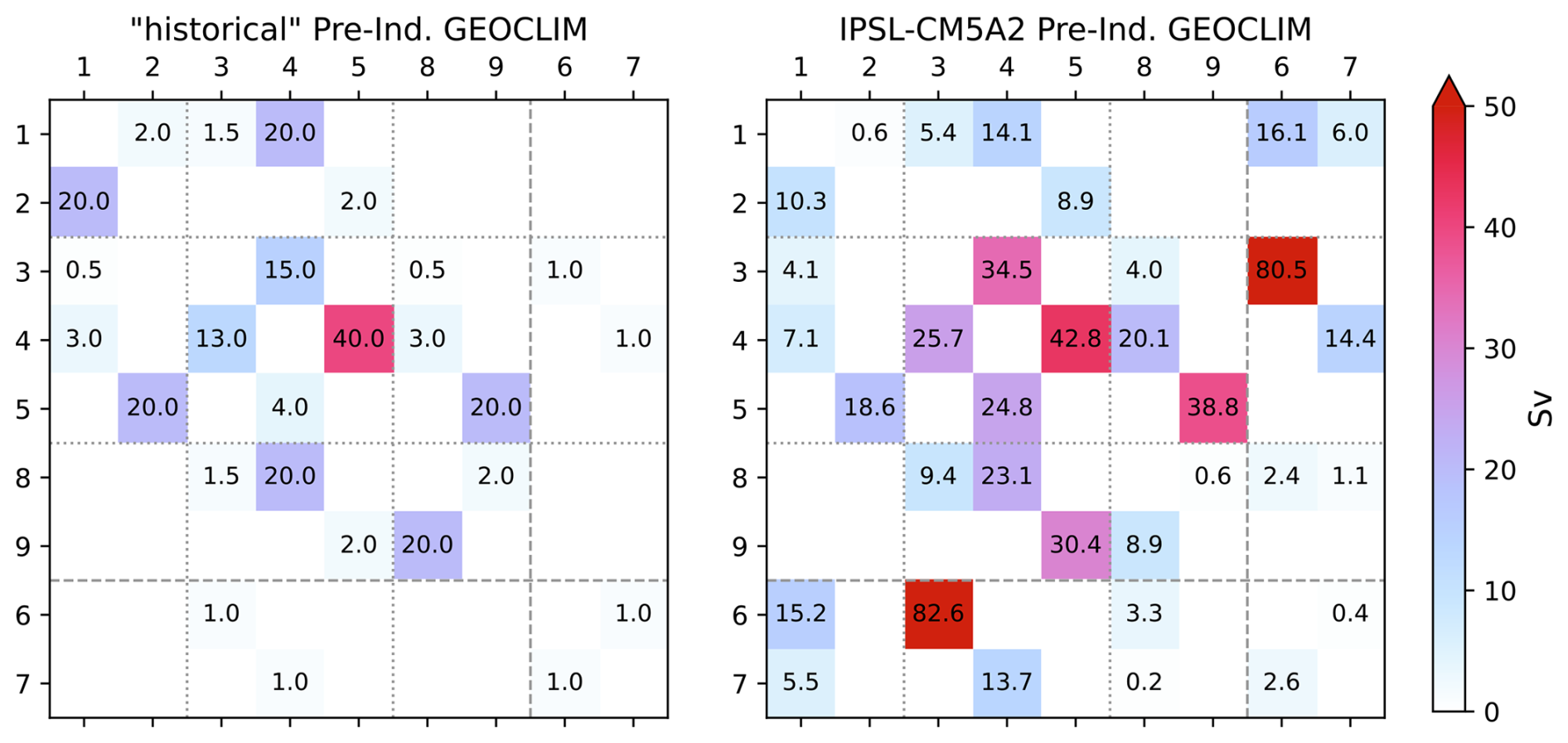
Figure C1 Flux matrices W representing oceanic circulation between GEOCLIM boxes in pre-industrial default nine-box GEOCLIM configuration. Fluxes are oriented from column i to line j. The numbering of boxes is the default GEOCLIM one (#1–2: N Hemisphere high latitudes (surface and deep), #3–4–5: midlatitude (surface, intermediate, and deep), #6–7: coastal oceans (surface and deep), #8–9: S Hemisphere high latitudes). However, the positions of the box pairs (6, 7) and (8, 9) have been swapped in the figure to better illustrate the distinction between “open-ocean” and “coastal” boxes.

Appendix D: Fourier analysis of oceanic oxygen time series in GEOCLIM Turonian experiment

This Appendix presents the Fourier transform analysis of the experiments presented in Sect. 4 (more specifically, Sect. 4.5). We computed the Fourier transforms of the 95–85 Ma time series of the three orbital parameters (Fig. D1a–c) and of the Arctic and North Atlantic open-ocean oxygen concentration of the corresponding GEOCLIM experiment (Fig. D1d–i). For all time series, the time average was removed before computing the fast Fourier transform. To identify the contribution of the three orbital parameters in the oxygen time series, we simply selected non-overlapping frequency ranges (colored in Fig. D1) and looked at the peaks within those frequency ranges in the oxygen Fourier transform.

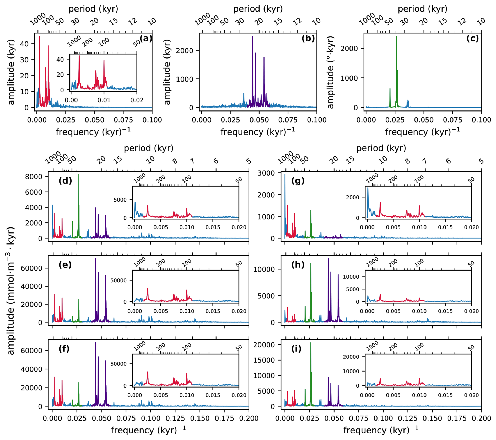
Figure D1 Amplitude spectrum of the Fourier transforms of the 95–85 Ma time series of orbital parameters and of open-ocean oceanic oxygen concentration from the 95–85 Ma GEOCLIM transient simulation (see Sect. 4.5). (a) Eccentricity, (b) cosine of precession angle ω, (c) obliquity, (d) O₂ in the surface (0–100 m) Arctic, (e) O₂ in the intermediate (100–900 m) Arctic, and (f) O₂ in the deep (900 m–bottom) Arctic; (g–i) same as (d–f) for the North Atlantic. Small encapsulated panels are close-ups of the 0–0.02 kyr⁻¹ frequency range for the corresponding bigger panels. Minor ticks on the “period” axis are every 1 kyr up to 20 kyr, every 10 kyr up to 100 kyr (200 kyr in the close-up panel), and every 100 kyr from 200 kyr to 1 Myr in the close-up panel. The non-overlapping frequency ranges associated with each orbital parameter are colored in red (eccentricity), violet (precession), and green (obliquity).