The updated Multi-Model Large Ensemble Archive and the Climate Variability Diagnostics Package: new tools for the study of climate variability and change

Observations can be considered as one realisation of the climate system that we live in. To provide a fair comparison of climate models with observations, one must use multiple realisations or ensemble members from a single model and assess where the observations sit within the ensemble spread. Single model initial-condition large ensembles (LEs) are valuable tools for such an evaluation. Here, we present the new Multi-Model Large Ensemble Archive (MMLEAv2) which has been extended to include 18 models and 16 two-dimensional variables. Data in this archive have been remapped to a common 2.5 × 2.5° grid for ease of inter-model comparison. We additionally introduce the newly updated Climate Variability Diagnostics Package version 6 (CVDPv6), which is designed specifically for use with LEs. The CVDPv6 computes and displays the major modes of climate variability as well as long-term trends and climatologies in models and observations based on a variety of fields. This tool creates plots of both individual ensemble members, and the ensemble mean of each LE, including observational rank plots, pattern correlations, and root mean square difference metrics displayed in both graphical and statistical output that is saved to a data repository. By applying the CVDPv6 to the MMLEAv2, we highlight its use for model evaluation against observations and for model intercomparisons. We demonstrate that for highly variable metrics a model might evaluate poorly or favourably compared to the single realisation the observations represent, depending on the chosen ensemble member. This behaviour emphasises that LEs provide a much fairer model evaluation than a single ensemble member, ensemble mean, or multi-model mean. By leveraging the combination of the CVDPv6 and MMLEAv2 presented in this paper we can determine which climate variables need a LE for fair assessment against observations.

1 Introduction

Single model initial-condition large ensembles (LEs) are a powerful tool for understanding past, current, and future climate (e.g. Deser et al., 2020; Maher et al., 2021a). A single LE allows for both the quantification and separation of the modelled forced response (response of any given variable to external forcing) and unforced internal variability, while the availability of multiple LEs additionally enables the assessment of model differences in both quantities (Deser et al., 2020; Lee et al., 2021; Maher et al., 2021b; Wood et al., 2021; Maher et al., 2023). LEs also facilitate a robust evaluation of individual climate models in comparison to observations, as they include a range of possible climate realisations (Goldenson et al., 2021; Suarez-Gutierrez et al., 2021; Labe and Barnes, 2022). Observations can be considered as one realisation of the climate system, and as such the interpretation of its comparison to a single historical simulation from a climate model, an ensemble mean, or multi-model mean is complicated. To this point, fairly evaluating projections in single runs of climate models, particularly for highly variable climate quantities against this single realisation of the real world is only possible by taking long time averages, to effectively smooth out natural climate variability, and allowing for the assessment of the model's forced response. The advantage of using a LE is that we can additionally evaluate whether observations sit within the model's ensemble spread. This is a necessary, although not sufficient, condition for model evaluation that makes LEs invaluable tools for such evaluation. The value of LEs derives from their large sample size. In addition to providing a range of plausible outcomes arising from the superposition of forced response and internal variability, the value of LEs derives from the sheer volume of data that they provide, enabling robust statistics on climate variability. For example, 250 years of simulation (e.g. 1850–2100) in a LE of only 20 members yields 5000 years of data for analysis, while a typical pre-industrial control simulation (piControl) provides 500–2000 years of output.

While evaluating whether the observations sit within the model spread is crucial for model evaluation, as it takes into account the fact that observations are only one possible realisation of the Earth system, understanding whether a model's forced response and internal variability are similar to observations is also vital. Quantifying the forced response and internal variability in observations is non-trivial and an active area of research. Ongoing efforts such as the “Forced Component Estimation Statistical Method Intercomparison Project” (ForceSMIP) (Wills et al., 2025) are expected to provide guidance on how best to extract forced response and internal variability from the observational record. LEs are critical to such projects. Quantifying these metrics in LEs themselves is more straightforward, but can be limited by ensemble size. The ensemble size needed to quantify any given metric is found to be dependent on the metric itself and the acceptable error on the quantification (Milinski et al., 2020; Lee et al., 2021; Planton et al., 2024). Progress has been made in the assessment of these quantities in combination, in comparison to observations with studies such as Suarez-Gutierrez et al. (2021) using LEs and a rank histogram method to evaluate whether LEs have a realistic forced response and internal variability of annual temperatures compared to the observed record. Such evaluations are becoming increasingly possible with the lengthening observational record and increasing forced trends (Simpson et al., 2025). Additionally, further understanding of when the forced response (signal) is likely to emerge from the internal variability (noise) is vital to understanding the climate we observe (e.g. Hawkins and Sutton, 2012). This concept is important for climate communication and quantifying when we expect to see climate change signals appear in our observed record. This is another avenue where LEs are vital tools to further research in the area (e.g. Schlunegger et al., 2020). Finally, the recent discovery of the signal-to-noise paradox (Scaife and Smith, 2018), where an ensemble can better predict observations than their own members, is also an avenue where LEs can provide valuable insight into model behaviour (Weisheimer et al., 2024).

The Multi-Model Large Ensemble Archive (MMLEA; Deser et al., 2020) was the first compilation of many LEs. The overview paper has been cited over 690 times despite only being published in 2020 (5 years ago; data as of 4 July 2025). This highlights the community's need for and the value of such an archive. In this paper, we present the MMLEAv2 archive that has been expanded beyond the original MMLEA to both include more models (18 compared to the original 7, largely those from the more recent CMIP6 archive), and 8 additional two-dimensional variables. The MMLEAv2 and a suite of observational datasets have also been regridded onto a 2.5° common horizontal grid to reduce data size, and to allow for straightforward model-to-model, and model-to-observations comparison. The MMLEAv2 allows for straightforward comparison between multiple models, and observations, with scope for scientists to download additional data on the native grids from the original data sources to supplement analysis.

The MMLEAv2 is an ensemble of opportunity, including both CMIP5- and CMIP6- class data, with no consistent forcing scenario available for all models. While this provides a limitation for the dataset, possibilities exist to compare warming levels rather than comparing across time (Seneviratne et al., 2021). This enables a more direct comparison between different scenarios, and circumvents this limitation, although it can only be implemented where the warming level itself, not the warming trajectory, is important (Hausfather et al., 2022).

An effective way to explore the characteristics of internal variability and forced response in the MMLEAv2 archive is to use the National Science Foundation National Center for Atmospheric Research Climate Variability Diagnostics Package Version 6 (CVDPv6; Phillips et al., 2020). Previous versions of this package have been used to investigate how modes of variability are represented over generations of CMIP climate models (Fasullo et al., 2020); questions of model evaluation robustness given the limited duration and certainty in observational datasets (Fasullo et al., 2024b); and strengths and weaknesses of US climate models in simulating a broad range of modes of variability (Orbe et al., 2020). In this study, we present the latest version of this package and highlight its value specifically for use with LEs, although it can also be applied to control simulations and models with one realisation. This automated package allows for model comparison with multiple observational datasets, as well as inter-model comparisons, with diagnostics completed over time periods of the user's choosing. The CVDPv6 provides an ensemble mean view in addition to individual member analysis. The ensemble mean view includes diagnostics of the forced component of climate variability and change, as well as metrics of the rank of the observations within the model ensemble spread to illustrate model bias. The package computes the leading modes of variability in the atmosphere and coupled ocean–atmosphere system including the El Niño–Southern Oscillation (ENSO), as well as long-term trends, climatologies, and a variety of climate indices. All results are saved in both graphical and numerical form, allowing for subsequent analysis and display. The user can specify any set of model LEs and observational datasets (including multiple datasets for a given variable) over multiple time periods for analysis. Additionally, the CVDPv6 offers a range of detrending methods that can be applied before computing diagnostics. The versatility of the CVDPv6 makes it an efficient and powerful tool for analysing LE output. In addition, the CVDPv6 displays information from all model simulations and observational datasets on a single page, facilitating model intercomparisons and assessment of observational uncertainty. In this paper, we will demonstrate the utility of the CVDPv6 as applied to the new MMLEAv2 and highlight some examples of its use and the insights derived therefrom. We note that multiple packages exist that provide ways to investigate climate model output. Examples include the Earth System Model Evaluation Tool (ESMValTool; Eyring et al., 2016), PCMDI Metrics Package (PMP; Lee et al., 2024), and Climate Model Assessment Tool (CMAT; Fasullo, 2020). An earlier version of the CVDP can be run through the ESMValTool and the CVDP can also be run from the Community Earth System Model (CESM) AMWG Diagnostics Framework (ADF) package and is planned to be run from within the CESM Unified Postprocessing and Diagnostics (CUPiD) package. Amongst many other uses, the CVDP is used alongside the CMAT package to evaluate CESM within the model's development cycle.

The aims of this paper are threefold:

1. Introduce the MMLEAv2 and describe the data available in this extended archive;

2. Demonstrate the utility of the CVDPv6 and the insights one can derive from it;

3. Highlight the importance of using LEs for model evaluation.

2 The MMLEAv2 dataset

The MMLEAv2 includes 18 models and 16 monthly variables as outlined in Table 1. The original MMLEA consisted of 7 CMIP5-class models with consistent historical and RCP8.5 forcing and 2 models with additional forcing scenarios. The MMLEAv2 contains 6 of the same models from the MMLEA as well as 12 additional CMIP6-class models. While a consistent RCP8.5 future forcing scenario was available for the CMIP5-class models, the CMIP6-class models use one or both of the historical plus SSP370 or SSP585 scenarios. Given that this is an ensemble of opportunity, whichever scenario was available and had the largest number of members is included in the MMLEAv2 (see Table 1). CMIP6-class model data are available for the period 1850–2100, except for GFDL-SPEAR-MED, which covers the time period 1921–2100. CMIP5-class data are available for a range of time periods, with the longest simulation from 1850–2099 (MPI-GE) and the shortest from 1950–2100 (CanESM2). The LEs have a minimum of 14 ensemble members for the historical period and a maximum of 100 members. In addition to the original variables in the MMLEA [precipitation (pr), sea level pressure (psl), surface air temperature (tas), horizontal wind stress in the u direction (tauu), horizontal wind stress in the v direction (tauv), sea surface height (zos), 500 mbar geopotential height (zg500)], the MMLEAv2 provides sea surface salinity (sos), evaporation (evspsbl), mixed-layer depth (mlotst), sea ice concentration (siconc/sic), 20° isotherm depth (a proxy for thermocline depth; z20), and 3 monthly extreme indices computed from daily data. We note that unlike the MMLEA, the MMLEAv2 does not provide surface radiative variables. The 3 monthly extreme indices (Zhang et al., 2011) are the monthly maximum of the daily maximum temperature (TXx), the monthly minimum of the daily minimum temperature (TNn), and the monthly maximum of the daily precipitation (Rx1day); they are computed from daily tasmax, tasmin, and pr data using the monmax and monmin functions in Climate Data Operators (CDO;  Schulzweida, 2023).

Ziehn et al. (2020)Kirchmeier-Young et al. (2017)Swart et al. (2019b)Kay et al. (2015)Rodgers et al. (2021)Jeffrey et al. (2012)Stevenson et al. (2023)Fasullo et al. (2024a)Döscher et al. (2022)Wyser et al. (2021)Sun et al. (2018)Burger et al. (2022)Delworth et al. (2020)Boucher et al. (2020)Tatebe et al. (2019)Hajima et al. (2020)Maher et al. (2019)Olonscheck et al. (2023)Sellar et al. (2019)

Table 1 Data included in the MMLEAv2 dataset. The model and its reference, forcing type, length of simulation, and variables available are listed in the table. Model names in italics are CMIP6-generation models and forcing, while CMIP5-generation models and forcing are not italicised. The number of ensemble members available for each variable are listed in the table. The variables, scenarios, set number (sets of LEs we have artificially split the models into for intercomparison purposes), and ensemble size highlighted in italics are those used in the CVDPv6 tables and figures. Where an additional variable is listed in parentheses, the original variable was unavailable, and this variable is included in the archive to replace it (these are as follows: ts – surface temperature; u10/v10 – 10 m wind speed).

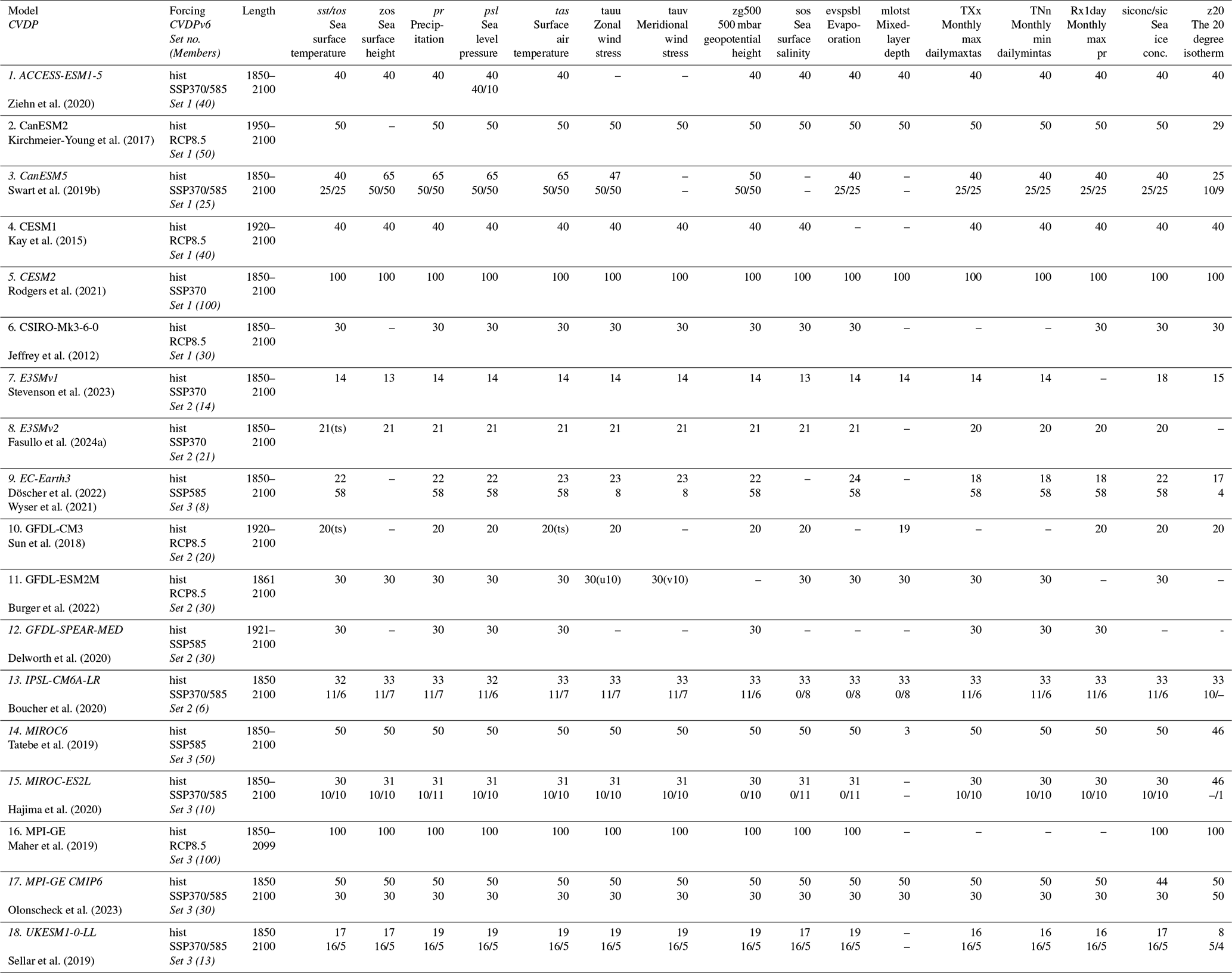
The MMLEAv2 data were remapped to a common 2.5 × 2.5° grid. CDO conservative mapping was used for pr, psl, tas, tauu, tauv, TXx, TNn, Rx1day, and zg500, whereas CDO's distance-weighted mapping was used for all other variables and for all variables in the CESM2 model due to an inability to use the other gridding tools on CESM2's native grid and psl in GFDL-CM3 due to an additional gridding issue. We note that for CESM2 z20 we regridded the full-depth temperature before calculating the 20° isotherm due to a gridding issue; for all other models the 20° isotherm was calculated prior to regridding. We also provide remapped observational datasets on the same common grid for ease of use as outlined in Table 2. We note that the data in the CESM models were shifted a month earlier to resolve the issue of netCDF readers reading the data 1 month off, which is an issue on the CESM native temporal grid. If possible, other variables that could be added to the archive in the future are winds at multiple pressure levels in the atmosphere, and surface and top-of-atmosphere fluxes. We note that while not in Table 1, GISS-E2-1-G is also available in the archive for the following variables (ensemble members in parentheses for hist/ssp370/ssp585): evspsbl, sos, zos (46/12/15); pr, psl, tas (46/22/10); tauu, tauv (46/17/10); mlotst (46/12/14); and tos (40/21/10). We note that this ensemble has multiple physics versions as described by the p flag in the ensemble number. This means that this ensemble is a combination of an initial condition and a perturbed parameter ensemble. It has been added to the archive as we believe its comparison will be useful compared to other ensembles, but note that it should not be treated the same way as the other SMILEs and as such is not included in Table 1 (see https://data.giss.nasa.gov/modelE/cmip6/, last access: 15 September 2025, for additional details) (Kelley et al., 2020).

Data are available at https://rda.ucar.edu/datasets/d651039/ (last access: 15 September 2025) with details of the data found on the project website https://www.cesm.ucar.edu/community-projects/mmlea/v2 (last access: 15 September 2025). The sources for downloading additional variables or the original data on the native grids are as follows:

• The Earth System Grid Federation (ESGF) Nodes for the CMIP6 Archive (https://esgf.github.io/nodes.html, last access: 15 September 2025); ACCESS-ESM1-5 (Ziehn et al., 2020, 2019), CanESM5 (Swart et al., 2019b, a), EC-Earth3 (Döscher et al., 2022; Wyser et al., 2021; EC-Earth, 2019), IPSL-CM6A-LR (Boucher et al., 2020, 2018), MIROC6 (Tatebe et al., 2019; Tatebe and Watanabe, 2018), MIROC-ES2L (Hajima et al., 2020, 2019; Tachiiri et al., 2019), UKESM1-0-LL (Sellar et al., 2019; Mulcahy et al., 2022), and GISS-E2-1-G (Kelley et al., 2020).

• The MMLEA (https://www.cesm.ucar.edu/community-projects/mmlea, last access: 15 September 2025); CanESM2 (Kirchmeier-Young et al., 2017), CESM1 (Kay et al., 2015; Deser and Kay, 2014), CSIRO-Mk3-6-0 (Jeffrey et al., 2012), GFDL-CM3 (Sun et al., 2018), and MPI-GE (Maher et al., 2019) with additional data available for the following models:

  • -

    CanESM2; https://crd-data-donnees-rdc.ec.gc.ca/CCCMA/products/CanSISE/output/CCCma/CanESM2/ (last access: 15 September 2025);

  • -

    CESM1; https://rda.ucar.edu/datasets/d651027/ (last access: 15 September 2025);

  • -

    MPI-GE; https://esgf-metagrid.cloud.dkrz.de/ (last access: 15 September 2025); then select project MPI-GE from the top left panel.

• The CESM2 Large Ensemble (https://www.cesm.ucar.edu/community-projects/lens2, last access: 15 September 2025; CESM2; Rodgers et al., 2021; Danabasoglu et al., 2020).

• The DKRZ node of the ESGF (https://esgf-metagrid.cloud.dkrz.de/, last access: 15 September 2025); MPI-GE-CMIP6 (Olonscheck et al., 2023).

• The GFDL SPEAR Large Ensembles (https://www.gfdl.noaa.gov/spear_large_ensembles/, last access: 15 September 2025); GFDL-SPEAR-MED (Delworth et al., 2020).

• The Energy Exascale Earth System Model (E3SM) large ensembles (https://aims2.llnl.gov/search/cmip6/?institution_id=UCSB&?experiment_id=historical,ssp370, last access: 15 September 2025 and https://portal.nersc.gov/archive/home/c/ccsm/www/E3SMv2/FV1/atm/proc/tseries/month_1, last access: 18 June 2025); E3SMv1 (Stevenson et al., 2023; Bader et al., 2019) and E3SMv2 (Fasullo et al., 2024a; Bader et al., 2022).

• The MMLEAv2 Archive (this published archive; https://rda.ucar.edu/datasets/d651039/, last access: 15 September 2025); GFDL-ESM2M (Burger et al., 2022).

We ask that this paper and the appropriate references from Table 1 (for each model used) are cited when using the MMLEAv2 data.

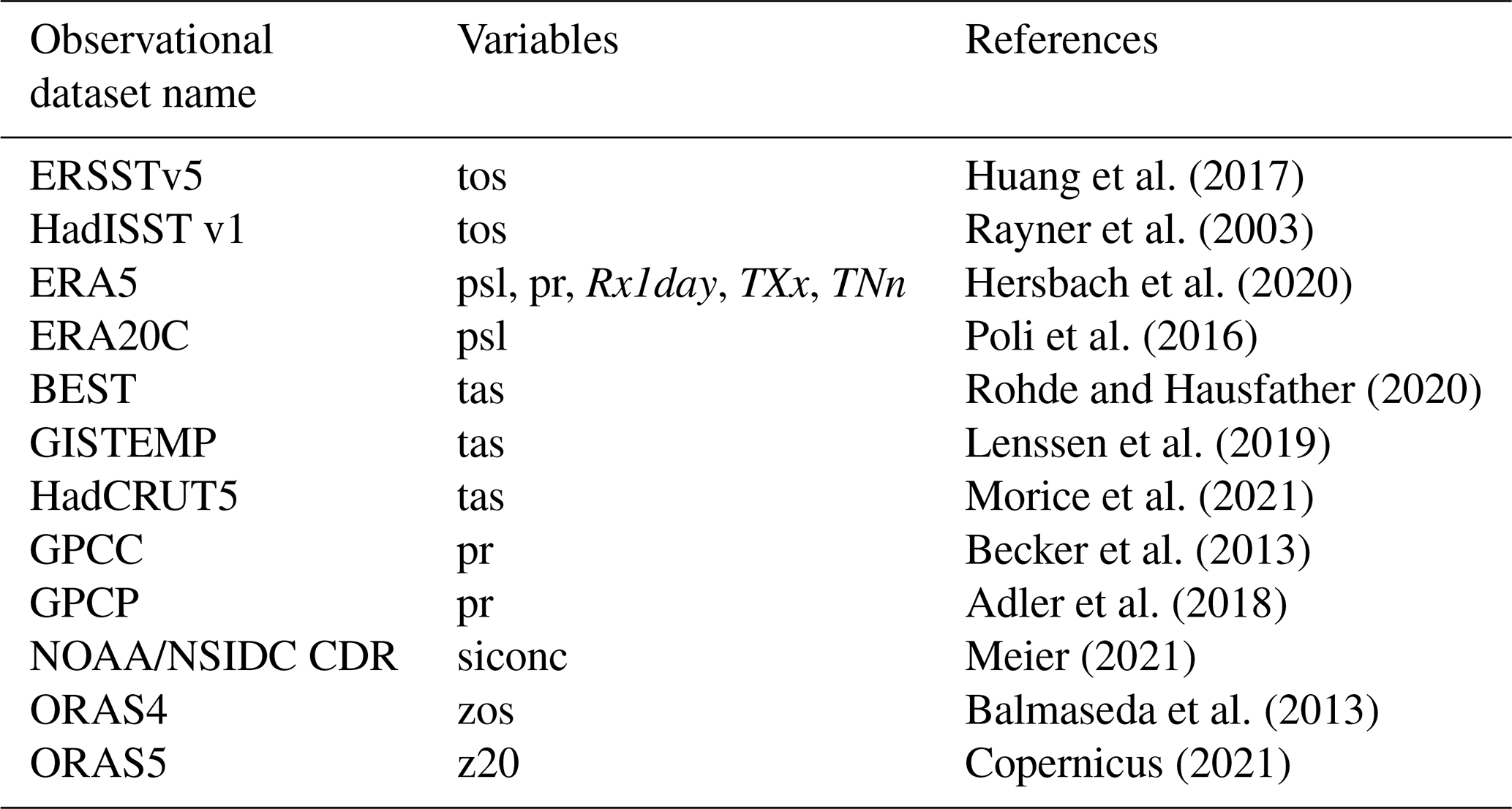
Huang et al. (2017)Rayner et al. (2003)Hersbach et al. (2020)Poli et al. (2016)Rohde and Hausfather (2020)Lenssen et al. (2019)Morice et al. (2021)Becker et al. (2013)Adler et al. (2018)Meier (2021)Balmaseda et al. (2013)Copernicus (2021)

Table 2 List of observational datasets used within the MMLEAv2 CVDPv6 comparisons. Additional datasets not used in the CVDPv6 are included in italics. Note all tas reference datasets are blended products that use surface air temperature over land and sea surface temperatures over the oceans.

3 The new CVDPv6

3.1 Scope of the package

The original Climate Variability Diagnostics Package (CVDP; Phillips et al., 2014) and the related Climate Variability and Diagnostic Package for Large Ensembles (CVDP-LE; Phillips et al., 2020) have been merged into a single application that incorporates the functionality of both packages. This merged application (henceforth referred to as the CVDPv6) is an automated analysis and graphics tool that facilitates the exploration of modes of climate variability and change in models, including LEs and observations. The CVDPv6 is written in NCL (the NCAR Command Language), which can be installed on most commonly used operating systems. The CVDPv6 computes and displays the major modes of climate variability as well as long-term trends and climatologies in models and observations based on a variety of fields including sea surface temperature (sst/tos), surface air temperature (tas), sea level pressure (psl), precipitation (pr), sea ice concentration (sic), sea surface height (zos), and the Atlantic Meridional Overturning Circulation (AMOC). As an analysis tool, it can be used to explore a wide range of topics related to unforced and forced climate variability and change. It can also help with formulating hypotheses, serve as a tool for model evaluation, and generally facilitate curiosity-driven scientific inquiry.

When the CVDPv6 is applied to LEs, it computes metrics that are unique to LEs; for example, the ensemble mean (an estimate of the forced response) and the ensemble spread due to internal variability. The CVDPv6 operates on a user-specified set of model simulations, observational datasets, and time periods, and saves the output (png graphical displays and netCDF data files) to a data repository for later access and further analysis. The CVDPv6 also provides the ability to view the output from two perspectives: Individual Member and Ensemble Summary (details provided below). A novel feature of the CVDPv6 is the option to detrend the data using one of four methodologies: linear, quadratic, 30-year high pass filter, and for model LEs, the removal of the ensemble mean. While removing the ensemble mean effectively removes the response to the modelled external forcing, the other methodologies are only effective at removing the long-term trend. The inclusion of multiple methods allows for the package to be used as a test-bed for the efficacy of the various observational detrending methods in separating the forced response from the internal variability, providing important information about how to interpret the results when the methods are applied to observations. Another novel feature of the CVDPv6 is that the reference dataset against which the model LEs are compared can be an observational product or the ensemble mean of an individual LE or multiple LEs at the user's discretion. These novel features of the CVDPv6 could be combined, for example, to show the detrended standard deviations of a variable such as surface temperature in future projections with reference to those in the historical period, enabling an assessment of forced changes in the characteristics of the modelled internal variability. To compare the MMLEAv2 archive to the observed historical climate, multiple observational datasets were downloaded and used as reference data within the CVDPv6 comparisons. The observational reference datasets are listed in Table 2. We note that while these data have been regridded as part of the MMLEAv2, the CVDPv6 does not need input files to be on a common grid for its use as the package does regridding on the fly. Compared to the previous version of the CVDP, the new CVDPv6 has some important improvements. It now includes a new Interdecadal Pacific Variability (IPV) Index (Henley et al., 2015); the Pacific Decadal Variability (PDV) and Atlantic Multidecadal Variability (AMV) definitions have been updated so that the global-mean SST anomaly is no longer removed following Mantua et al. (1997) and Deser and Phillips (2023), respectively. Additionally, regression maps for multiple variables have been added for AMV, PDV, and both IPV versions and sea surface height (zos) has been added to the list of variables for the climatological averages, standard deviation, and trend maps. Finally, a number of new regional time series have been added.

3.2 CVDPv6 output

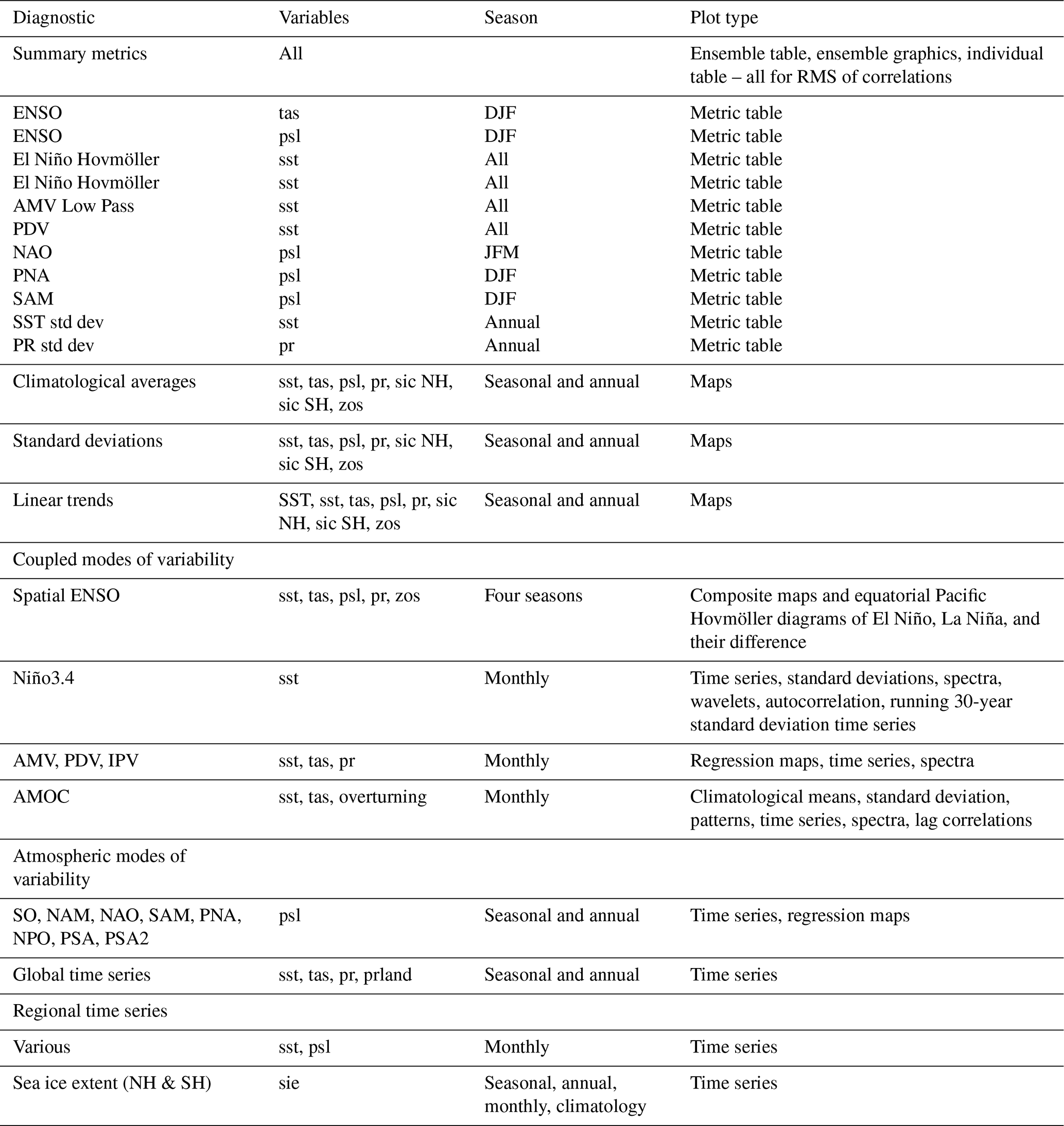
A list of the output from the CVDPv6 can be found in Table 3. A detailed description of each output field is provided in the Supplement. All calculations performed in the CVDPv6, including definitions of the modes of variability, are given in the Methodology and Definitions link at the top of the CVDPv6 output web page (https://webext.cgd.ucar.edu/Multi-Case/MMLEA_v2/, last access: 15 September 2025). A number of summary metrics accompany the graphical displays (see Table 3 for a listing). In particular, for each spatial map, the pattern correlation between the model simulation (which could be an individual member of a LE in the Individual Member view or the ensemble mean of a LE in the Ensemble Summary view) and the reference dataset (typically observations) is given in the upper right of the map. In addition, for modes of variability based on the empirical orthogonal function (EOF) analysis, the fractional variance explained is also provided. The rank maps in the Ensemble Summary view, which show the rank of the reference dataset within the ensemble spread of the LE, also provide a summary metric of the fractional area of the globe with values between 10 % and 90 %. For each time series displayed in the Ensemble Summary view, the ensemble mean and the 25th–75th and 10th–90th percentile ranges across the ensemble members are shown, along with the 10th, 50th, and 90th percentile values for linear trends. The percentage of time that the reference dataset lies within the 10th–90th percentile range of the LE values is also shown. The package also produces a synthesis of model performance based on pattern correlations and root mean square (RMS) difference for 15 key spatial metrics of climate variability (listed in Table 3) as well as an overall benchmark based on a mean score of all 15 metrics combined. These summaries are provided in both graphical and tabular format. A novel feature of the summary table is the ability to sort the values according to a particular metric (for example, the North Atlantic Oscillation; NAO) or by the mean score across the 15 metrics. The 10th and 90th percentile values for each metric and the mean score are also provided in the tables for each model LE, facilitating model performance intercomparisons. The package also produces a range of output (listed in Table 3) that can be viewed in the Individual Member or in the Ensemble Summary view. The Individual Member view gives the option for each ensemble member to be plotted in its native state or as a bias plot compared to a reference dataset (e.g. observations). The Ensemble Summary view plots the ensemble mean, the reference dataset, the difference between the two, and the rank of the reference within the ensemble. If the model and the reference agree well one would expect the reference to sit at a rank inside the model spread, i.e. within the 10 % and 90 % range, 80 % of the time (Suarez-Gutierrez et al., 2021; Phillips et al., 2020). The rank plot enables a quick evaluation of the variable or metric plotted.

Table 3 Contents of the CVDPv6. In addition to the information summarised in this table, the CVDPv6 displays pattern correlations against the reference dataset and the areal fraction of rank values within 10 %–90 % for all diagnostics plotted in map form. It also provides the temporal fraction of rank values within 10 %–90 % and an ensemble mean summary plot for all diagnostics plotted in time series form. For the modes of variability computed using an EOF analysis, a graphical summary of the distribution of percent variance explained (PVE) values across the entire ensemble appears above the numerical values of PVE (10th, 50th, and 90th). Details of these modes and how they are calculated are found in the Supplement.

3.3 CVDPv6 applied to MMLEAv2

We have run several applications of the CVDPv6 on the MMLEAv2; the output can be found at https://webext.cgd.ucar.edu/Multi-Case/MMLEA_v2/ (last access: 15 September 2025). In particular, we provide a version without detrending and one where the observations have been quadratically detrended and the LEs have been detrended by removing the ensemble mean as this explicitly removes the forced response from each LE (note that detrending is omitted from the calculations of climatologies and trends). The CVDPv6 comparisons are divided into three sets of models (see Table 1 for which model is in which set) for ease of visualisation. The CVDPv6 is run on each of the three sets of models for the time periods 1950–2022 and 2027–2099. An additional set named Set123 only includes the summary metrics (tables and graphics) to facilitate an inter-model comparison across the entirety of the MMLEAv2. All analysis was completed on RCP8.5 and SSP5-8.5 except for E3SMv1, E3SMv2, CESM2, and UKESM1-0-LL where SSP3-7.0 was used. The observational datasets used for these comparisons are shown in Table 2.

4 Inter-model comparison tables and graphics

This section demonstrates the inter-model comparison tables and graphics from the CVDPv6 for all MMLEAv2 ensemble members and the types of conclusions that can be drawn from them.

Multiple evaluation methods exist to compare climate variability in models with observations. While they do not always provide consistent answers, together they can be used to create a more general picture of model performance. Here, we use two complementary evaluation methods: pattern correlations (Fig. 1) and RMS differences (Fig. 2). The pattern correlation informs about the spatial similarity between two maps, while the RMS provides a summary of the relative amplitude of the maps. For the pattern correlation mean score, CESM2 and GFDL-SPEAR have the highest individual ensemble member scores compared to observations (around 0.9), followed by a group of models clustered with their highest correlation in the 0.8–0.85 range. For the RMS, the highest performance (lowest RMS values) are found again for GFDL-SPEAR, but also EC-Earth3 and UKESM1-0-LL. These results demonstrate that GFDL-SPEAR is a high performer for both spatial pattern and amplitude. However, it is worth keeping in mind that the evaluation is also metric-dependent. For example, ACCESS-ESM1-5 has one of the lowest RMS scores and high correlations for ENSO TAS in DJF, showing it performs well in both pattern and amplitude for this metric. However, for the La Niña Hovmöller, it is in the bottom two models for the spatial pattern. Another example is GFDL-CM3, which has the lowest PR STD correlation, but conversely performs relatively well on amplitude for the PNA metric. This demonstrates that models can perform well for one metric and evaluation type, but poorly for another, meaning that one must be careful in selecting an evaluation method and metric fit for purpose for any given study.

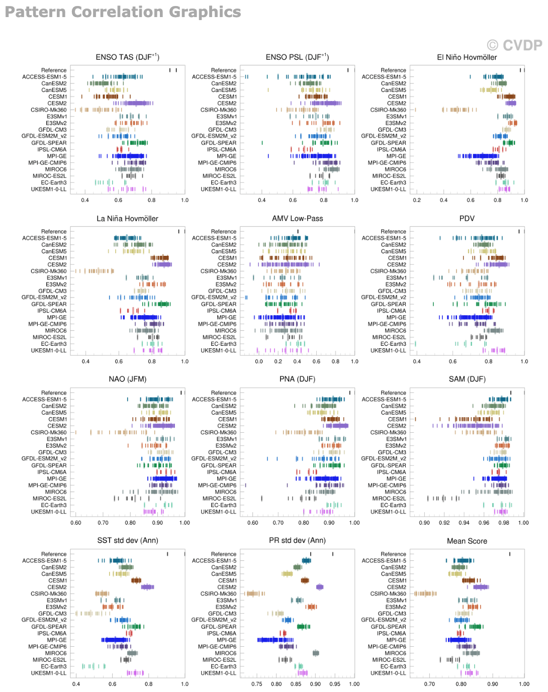
Figure 1 The pattern correlation of each ensemble member of all MMLEAv2 models with the first specified observational dataset (for each variable for each metric) compared to every other specified observational dataset and every model simulation in this figure directly from the CVDPv6. Shown for multiple modes of variability, the standard deviation of sst and pr, and a mean score across all metrics used in the figure (after applying a Fisher z transform). Computations are completed over the period 1950–2022. Observations are detrended using a quadratic fit, while the LEs are detrended by removing the ensemble mean. Note that all of the metrics shown in Figs. 1 and 2 are spatial patterns. For example, “ENSO TAS (DJF+1)” is the spatial map of TAS anomalies in DJF+1 based on ENSO (e.g. El Niño minus La Niña) composites, “PR std dev (Ann)” is the map of the PR standard deviation based on annual means, and “El Niño Hovmöller” is the Hovmöller diagram of El Niño composites of Equatorial Pacific SST anomalies over the longitude domain 120° E–80° W and time domain January year 0 – May year+2 (see the Methodology and Definitions link in the CVDPv6). The following domains are used to compute the pattern correlations: global for standard deviations, ENSO, and PDV; 63° S–65° N for AMV; 120° E–80° W and January year 0 – May year+2 for El Niño and La Niña Hovmöllers; 20–90° N for NAM/NAO; and 20–90° S for SAM.

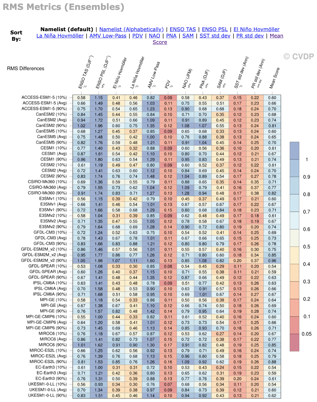
Figure 2 The RMS difference between each MMLEAv2 model ensemble average and observations as well as the 10th and 90th percentile of the RMS difference across the ensemble (shown in both colours and numbers in the table). Shown for multiple modes of variability, the standard deviation of sst and pr, and a mean score across all metrics used in the figure (after normalising each by the spatial RMS of the observed pattern to account for the different units of each variable). Computations are completed over the period 1950–2022. Observations are detrended using a quadratic fit, while the LEs are detrended by removing the ensemble mean. Area-weighted pattern correlations and RMS differences are calculated between observations and each model simulation (regridded to match the observational grid) for 11 climate metrics. The Total Score column shows the average of the 11 pattern correlations (z-transformed) and RMS differences. The following domains are used to compute the RMS differences: global for standard deviations, ENSO, and PDV; 63° S–65° N for AMV; 120° E–80° W and Jan year 0 – May year+2 for El Niño and La Niña Hovmöllers; 20–90° N for NAM/NAO; and 20–90° S for SAM.

There are some metrics where all models tend to perform well or poorly. For example, the red columns of Fig. 2, PDV, SST STD, and PR STD, all show low error compared to observations in all models and ensemble members for the RMS. Conversely, the blue-coloured columns such as ENSO PSL and AMV Low Pass show poor performance across all ensemble members of all models. For the pattern correlation, again all models and members perform poorly for the AMV Low Pass where there is a maximum correlation of 0.6 (Fig. 1). On the contrary, no ensemble member of any model has a correlation below 0.88 for the Southern Annular Mode (SAM), highlighting high performance of all models for this metric. Metrics where all models perform poorly can tell us about general biases found in all climate models. The AMV Low Pass is an example of where the models perform poorly in both the spatial pattern and amplitude, although this could be due to the tendency of the AMV Low Pass Index to mix together multiple independent processes (Wills et al., 2019; Deser and Phillips, 2023; O’Reilly et al., 2023) which might have different relative weights in models and observations. On the flip side the low RMS for SST STD highlights that the amplitude of SST variability is generally correct in all models, while in many models the maximum correlation is below 0.8 and as low as 0.4, suggesting that while the amplitude is correct there is bias in the spatial pattern. Teasing out where consistent model biases exist and whether they appear for both pattern and amplitude can inform scientific research and model development to improve models in the coming model generations.

Ensemble members from the same model with the same external forcing can have a wide range of performance compared with observations. For metrics such as the AMV Low Pass, the pattern correlation with observations ranges from slightly negative to 0.6 in an individual model. ENSO TAS also has a range of possible correlations that vary by up to 0.3 between members. These examples highlight that for metrics such as these two, the use of a single ensemble member would not give a correct model evaluation. For other metrics such as PR STD, the range of correlations within a single model only varies by a magnitude of 0.1, demonstrating that in this case a LE is not necessary for model comparison to observations. The range of correlations across ensemble members is linked to the magnitude of internal variability of a metric relative to its ensemble mean (e.g. Milinski et al., 2020; Lee et al., 2021). This range is not determined solely by ensemble size, as demonstrated by the SAM metric, where the 100-member CESM2 model has a much larger range of possible correlations than the 100-member MPI-GE. This difference in range from two models with the same ensemble size does, however, demonstrate that the variability of a single metric can be model-dependent, similar to Lehner et al. (2020). Another example that highlights the importance of considering the full ensemble, rather than one member, is the El Niño Hovmöller, which for CESM2 can have a RMS as small as 0.49 and as large as 0.76. If the member with the 0.76 RMS was used this model would be deemed poor at representing the El Niño evolution, while the opposite conclusion would be made if the 0.49 member was selected. Similar results are again found for smaller ensembles with the PNA in ACCESS-ESM1-5 as low as 0.43 or as high as 0.68 depending on which member was chosen. In general, Figs. 1 and 2 highlight the importance of using LEs for model evaluation, particularly for metrics with high internal climate variability.

5 Model evaluation figures

This section gives examples of figures output from the CVDPv6 and associated insights that can be made into the MMLEAv2 models.

The CVDPv6 can be used to assess annual global average surface temperature and determine whether the response to external forcing (i.e. greenhouse gases, anthropogenic aerosols, and volcanic forcing) in combination with internal variability is similar to observations. For the Set 1 MMLEAv2 models shown in Fig. 3, only CESM2 and CESM1 largely encompass the observations within the model spread as highlighted by the temporal ranks (e.g. the percentage of time that the observed value lies within the 10th–90th percentile range of the model's ensemble members shown in the bottom left of the plots), where these models have 85 % and 79 %, respectively. ACCESS-ESM1-5, CanESM2, and CanESM5 all have a larger climate sensitivity than is estimated from observations, as demonstrated by all members, warming much more than the observations at the end of the historical period. The CSIRO-Mk360 model has a bias in the historical period where it does not warm from 1960–2000, dissimilar to what is observed. In response to volcanic forcing, all models have a distinctive dip in temperature in 1963 (Agung), 1982 (El Chichón), and 1991 (Pinatubo) that is similar in magnitude to the observed record, except CSIRO-Mk36 which does dip in response to eruptions, but at a different rate to observations. This suggests that the global-mean annual-mean temperature response to large tropical volcanic eruptions is realistic in most Set 1 models.

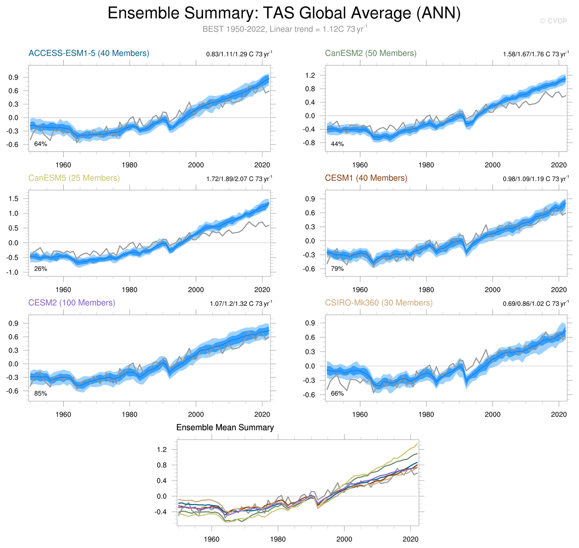
Figure 3 Global average surface air temperature anomalies for Set 1, computed annually over the period 1950–2022. The dark blue curve shows the model’s ensemble mean time series, and the dark (light) blue shading around this curves depicts the 25th–75th (10th–90th) percentile spread across the ensemble members. Observations are shown in the thick grey curve with the dataset name and trend of the period written in grey under the figure title. The last panel shows the ensemble mean of each LE (each model's line colour corresponds to the colour of each model's title in the previous panels of this figure) as well as observations. The 10th, 50th, and 90th percentile values of the linear trends across the model are shown in the top right of each panel and the percentage value on the bottom left of each panel is the percentage of time that the observed value lies within the 10–90th percentile of the LE values. Here, each vertical bar denotes a different ensemble member, and the 10th, 50th, and 90th percentile values are identified with taller bars. Sets 2 and 3 can be found here: https://webext.cgd.ucar.edu/Multi-Case/MMLEA_v2/MMLEA_Set2_nonenone_1950-2022/tas_global_avg_ann.summary.png (last access: 15 September 2025) and https://webext.cgd.ucar.edu/Multi-Case/MMLEA_v2/MMLEA_Set3_nonenone_1950-2022/tas_global_avg_ann.summary.png (last access: 15 September 2025).

Accurately representing large-scale modes of climate variability in models is important as these modes are key components of the climate system. The large-scale modes shown in the following examples were calculated after the removal of the ensemble mean. Hence they approximate pure internal variability with all external trends removed. This is a key use of LEs and a powerful tool within the CVDPv6. We note that changes in the variability itself due to external forcing are not removed using this methodology, so changes in the variability itself can be assessed using this method. The CVDPv6 uses a rank histogram approach where the rank of observations is shown within each model's spread. This type of comparison between observations and models is only possible using LEs. The NAO pattern in DJF for the Set 1 models is shown in Fig. 4. CESM2 and CanESM5 have the largest percentage of white area (indicating that observations lie in the centre of the distribution of the model's diagnosed internal variability patterns) in the rank histogram map (areal percentage of observed values lying within the 10th–90th percentile of the LE values of 61 % and 59 %, respectively), while CSIRO-Mk36 has the lowest at 28 %. For the most part, the Set 1 models tend to have similar biases, with the NAO variability overestimated in the North Pacific and over Alaska and underestimated in the North Atlantic and over most of Russia and Siberia. A similar plot for the PDV is shown in Fig. 5 for Set 3 models. In this case, the pattern biases are quite different for different models, especially in the tropical Pacific, where some models have too much PDV variability and some have too little. There is a consistent bias in the North Pacific, where all Set 3 models show too large Kuroshio-Oyashio Extension anomalies that are located too far north. EC-Earth3, MPI-GE, and MPI-GE-CMIP6 are the models with more than 60 % of the areal percentage of the ranks occurring between the 10th and 90th percentile, indicating that they capture the observed PDV best out of the Set 3 models. Modes of variability can also be assessed by their spectra (Fig. 6; ENSO spectra). For the ENSO spectra in Set 2 models, we find that GFDL-CM3, E3SMv2, and IPSL-CM6A have a peak that sits at 3 years, while observations have a broader 3–7 year peak. GFDL-ESM2M is similar to observations but with a stronger peak. GFDL-SPEAR and E3SMv1, however, are much more in agreement with observations, with the ensemble spread encompassing observations.

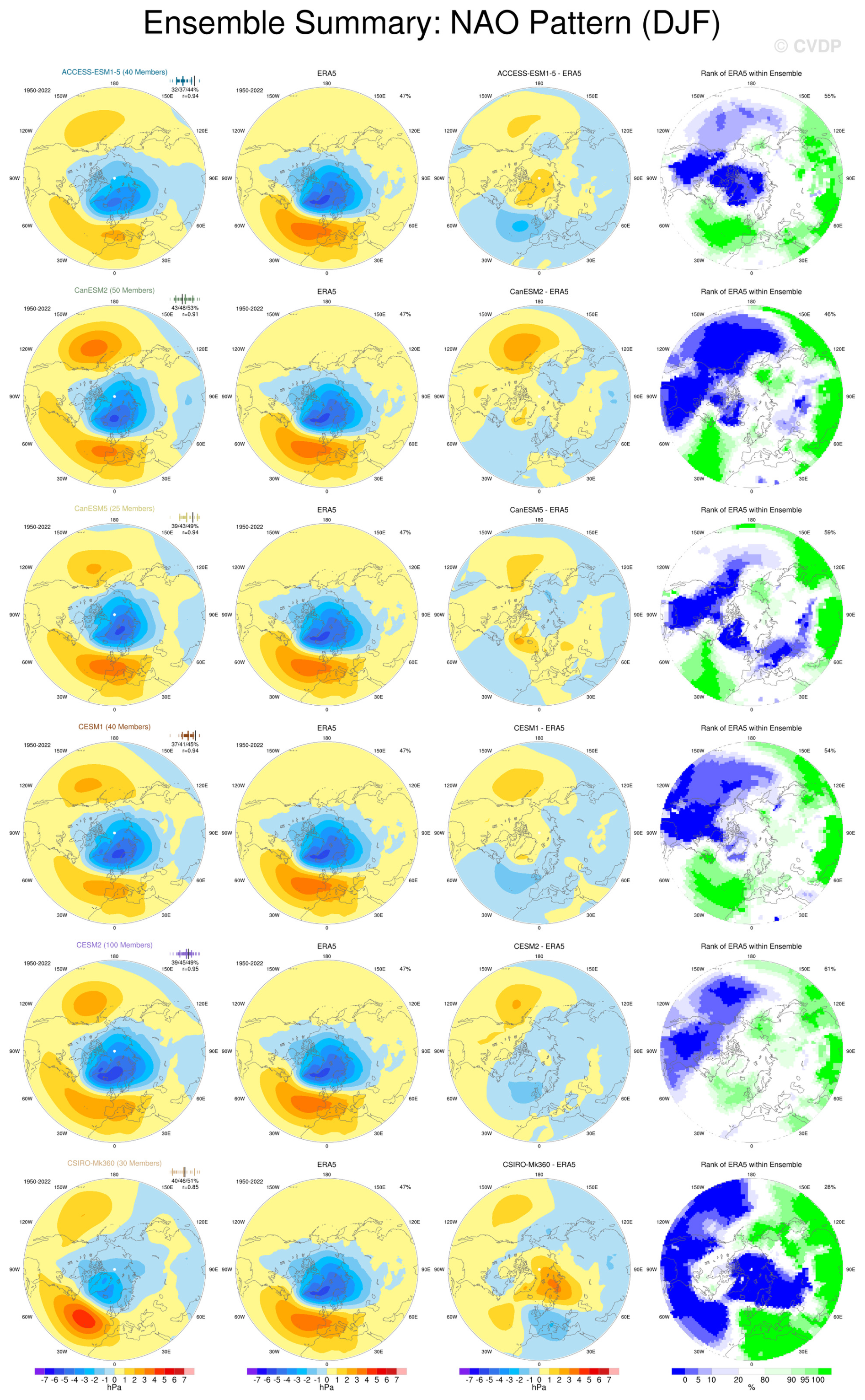
Figure 4 The North Atlantic Oscillation (NAO) pattern in DJF: (left) ensemble mean of Set 1 models, (middle left) observations, (middle right) difference between the ensemble mean and observations, and (right) rank of observations within the ensemble spread. The PVE by the NAO over its native (EOF) domain is given in the subtitle at the top right of the regression map: the first, second, and third values indicate the 10th, 50th, and 90th percentile values across the ensemble, respectively. A graphical summary of the distribution of PVE values across the entire ensemble appears above the numerical values of PVE: each vertical bar denotes a different ensemble member, and the 10th, 50th, and 90th percentile values are identified with taller bars. The observed PVE value is marked by a grey vertical bar. To quantify the degree of resemblance between the simulated and observed NAO regression maps, a pattern correlation (r) is computed between the observed NAO regression map and the ensemble average of the simulated NAO regression maps (e.g. maps in columns 1 and 2) over the domain shown. This r value is displayed at the upper right of each model panel, just below the range of PVE values. White areas on the observed percentile rank maps indicate regions where the observed value lies within 10 %–90 % of the model LE values, indicating the model is likely to be realistic. The value to the right of each rank map denotes the areal percentage of observed values lying within the 10th–90th percentile of the LE values. Computations are completed over the period 1950–2022. The NAO is the leading EOF in the region [20–80° N, 90° W–40° E] following Hurrell and Deser (2009). Observations are detrended using a quadratic fit, while LEs are detrended by removing the ensemble mean. Sets 2 and 3 can be found here: https://webext.cgd.ucar.edu/Multi-Case/MMLEA_v2/MMLEA_Set2_quadrmEM_1950-2022/npo_pattern_djf.summary.png (last access: 15 September 2025) and https://webext.cgd.ucar.edu/Multi-Case/MMLEA_v2/MMLEA_Set3_quadrmEM_1950-2022/nao_pattern_djf.summary.png (last access: 15 September 2025).

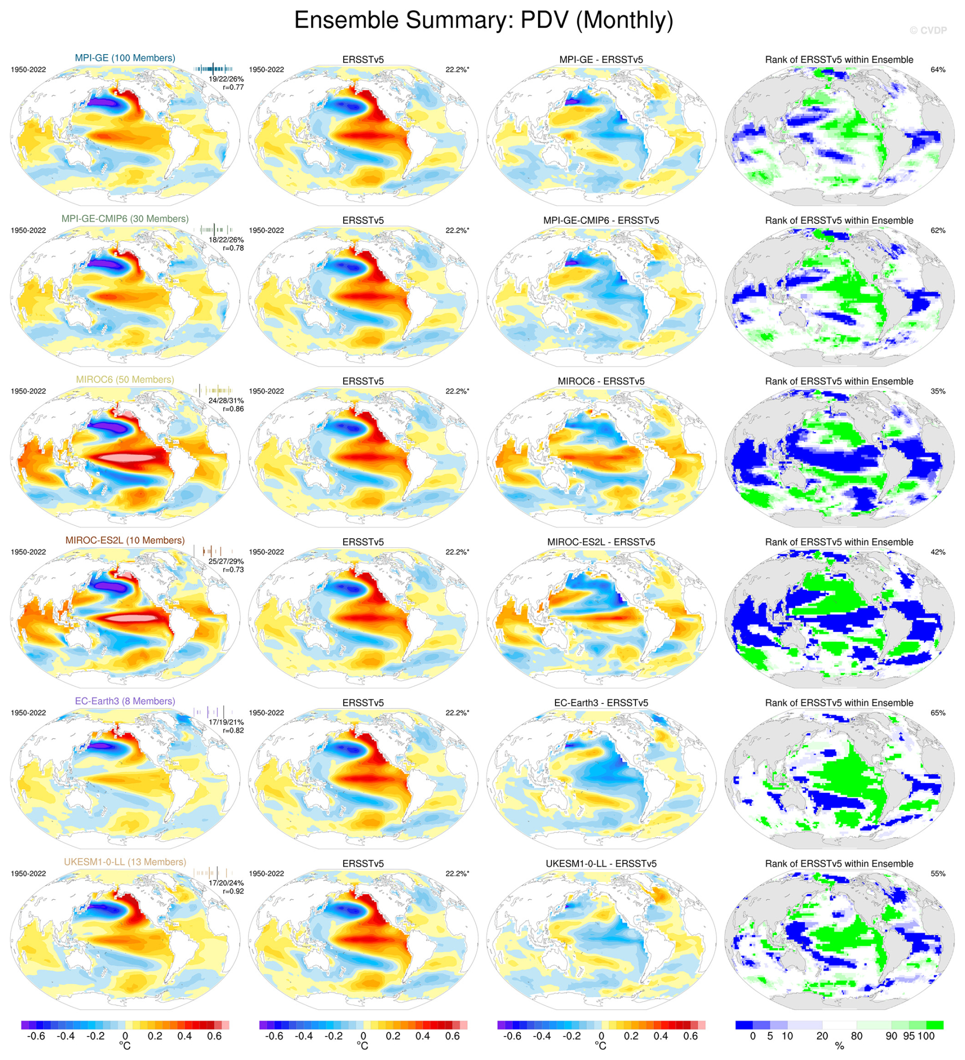
Figure 5 The PDV pattern in DJF: (left) ensemble mean of Set 3 models, (middle left) observations, (middle right) difference between the ensemble mean and observations, and (right) rank of observations within the ensemble spread. The PVE by the PDV over its native (EOF) domain is given in the subtitle at the top right of the regression map: the first, second, and third values indicate the 10th, 50th, and 90th percentile values across the ensemble, respectively. A graphical summary of the distribution of PVE values across the entire ensemble appears above the numerical values of PVE: each vertical bar denotes a different ensemble member, and the 10th, 50th, and 90th percentile values are identified with taller bars. The observed PVE value is marked by a grey vertical bar. To quantify the degree of resemblance between the simulated and observed PDV regression maps, a pattern correlation (r) is computed between the observed PDV regression map and the ensemble average of the simulated PDV regression maps (e.g. maps in columns 1 and 2) over the domain shown. This r value is displayed at the upper right of each model panel, just below the range of PVE values. White areas on the observed percentile rank maps indicate regions where the observed value lies within 20 %–80 % of the model LE values, indicating the model is likely to be realistic. The value to the right of each rank map denotes the areal percentage of observed values lying within the 10th–90th percentile of the LE values. Computations are completed over the period 1950–2022. The PDV Index is defined as the standardised principal component (PC) time series associated with the leading EOF of area-weighted monthly SST anomalies over the North Pacific region [20–70° N, 110° E–100° W] minus the global mean [60° N–60° S], following Mantua et al. (1997). Observations are detrended using a quadratic fit, while LEs are detrended by removing the ensemble mean. Sets 1 and 2 can be found here: https://webext.cgd.ucar.edu/Multi-Case/MMLEA_v2/MMLEA_Set1_quadrmEM_1950-2022/pdv.summary.png (last access: 15 September 2025) and https://webext.cgd.ucar.edu/Multi-Case/MMLEA_v2/MMLEA_Set3_quadrmEM_1950-2022/pdv.summary.png (last access: 15 September 2025).

Another important aspect of model evaluation is the consideration of how well a model represents the observed impacts of a mode of variability. In Fig. 7 we demonstrate the SON precipitation impacts from La Niña in the Set 3 models. MIROC6 has 70 % of the areal percentage of ranks between the 10th and 90th percentile, with all other models above 62 %. This shows that over 60 % of the globe has rainfall impacts in SON that are well represented in the Set 3 models. Be that as it may, biases do exist. For example, all models have a wet bias in the western tropical Pacific and the Alaskan coastline, and a dry bias over California in relation to observed La Niña events. In other regions models have differing biases, with the La Niña teleconnection to Australia overestimated in some models and underestimated in others. Whether these biases are due to model errors or uncertainty in the observed composite due to limited sampling of events (Deser et al., 2018, 2017) and/or data issues is less clear due to a sparsity of observations in some regions. While not shown in this paper, the CVDPv6 allows for comparison with multiple observational products, which can help characterise observational uncertainty.

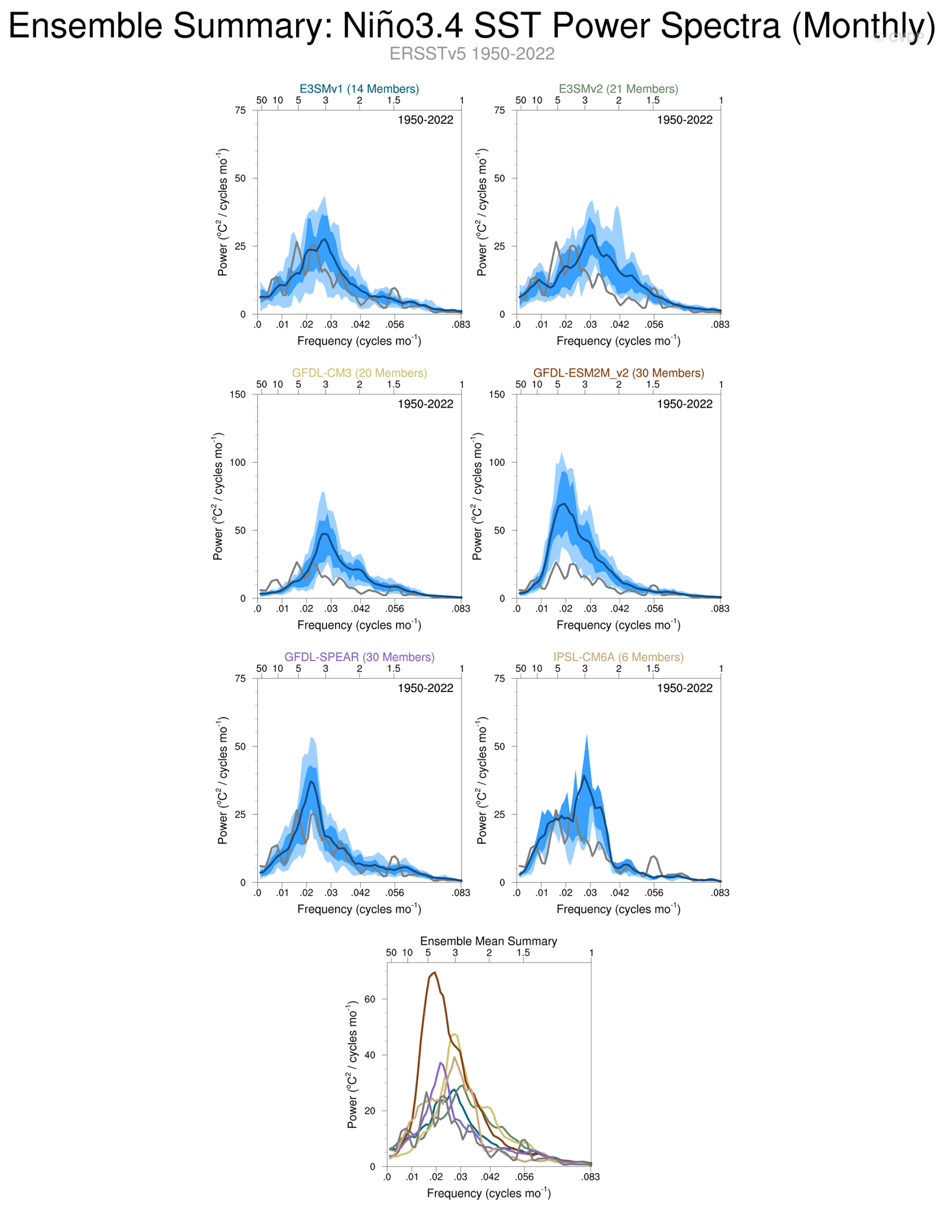
Figure 6 The ENSO (Niño3.4) monthly power spectrum for Set 2 models. The dark blue curve shows the model’s ensemble mean power spectrum, and the dark (light) blue shading around this curves depicts the 25th–75th (10th–90th) percentile spread across the ensemble members and the grey/brown line is the observations. The bottom right shows the ensemble mean from each model and the observations on a single panel. Computations are completed over the period 1950–2022. Power spectra are computed in variance preserving format from the linearly detrended December Niño3.4 SST Index (SST anomalies averaged over the region 5° N–5° S, 170–120° W). Observations are detrended using a quadratic fit, while LEs are detrended by removing the ensemble mean. Sets 1 and 3 can be found here: https://webext.cgd.ucar.edu/Multi-Case/MMLEA_v2/MMLEA_Set1_quadrmEM_1950-2022/nino34.powspec.summary.png (last access: 15 September 2025) and https://webext.cgd.ucar.edu/Multi-Case/MMLEA_v2/MMLEA_Set3_quadrmEM_1950-2022/nino34.powspec.summary.png (last access: 15 September 2025).

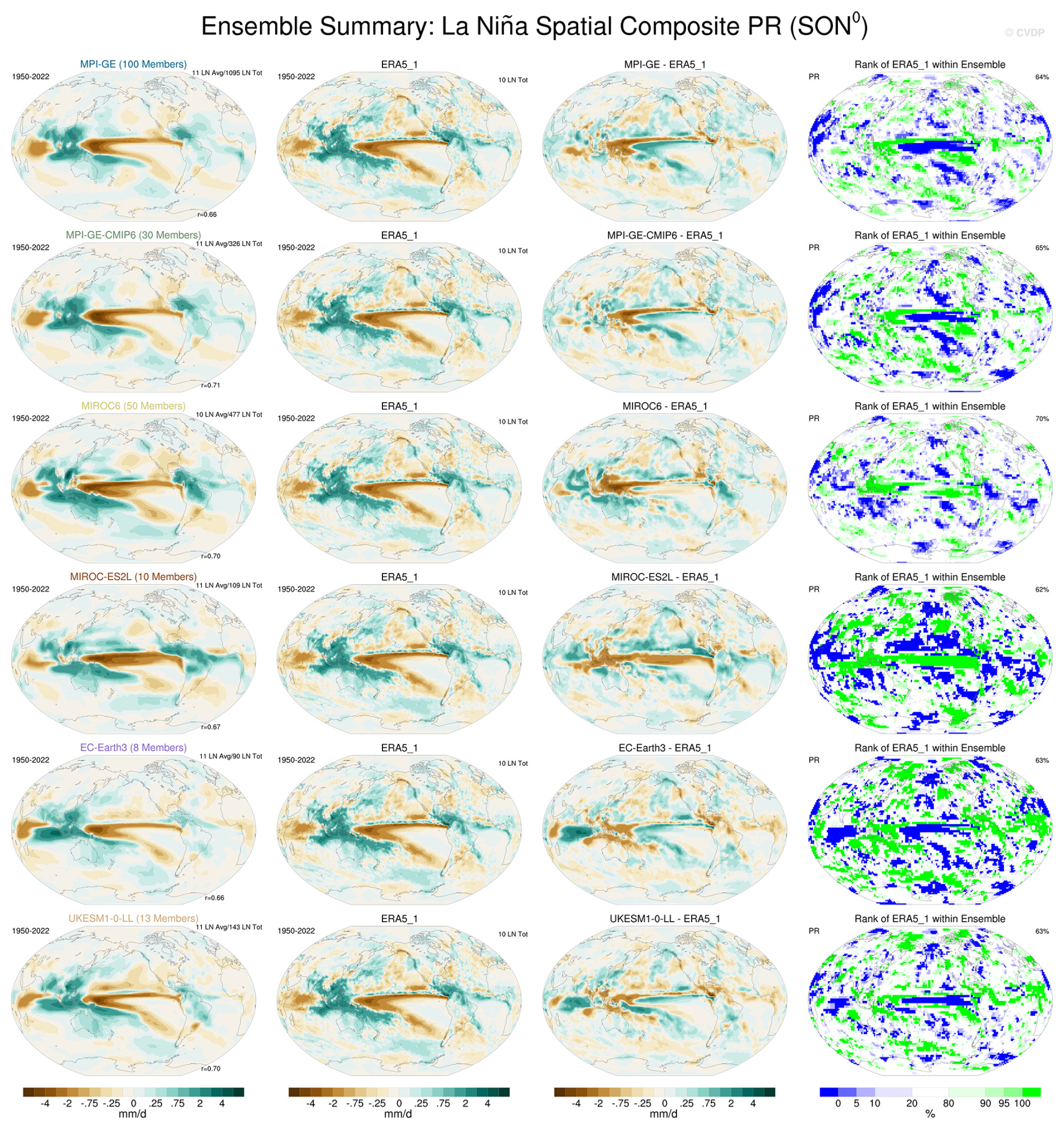
Figure 7 Composite of precipitation in SON for La Niña events: (left) ensemble mean of Set 3 models, (middle left) observations, (middle right) difference between the ensemble mean and observations, and (right) rank of observations within the ensemble spread. The top right of the rightmost panels shows the percentage of the map that is white, where observations are considered to be within the ensemble spread. Computations are completed over the period 1950–2022. The pattern correlations are displayed at the lower right of each model panel. The number of events that go into each spatial composite are displayed at the upper right of each panel (given as an average per ensemble member and as a total over all ensemble members). The value to the right of each rank map denotes the areal percentage of observed values lying within the 10th–90th percentile of the LE values. Observations are detrended using a quadratic fit, while LEs are detrended by removing the ensemble mean. Sets 1 and 2 can be found here: https://webext.cgd.ucar.edu/Multi-Case/MMLEA_v2/MMLEA_Set1_quadrmEM_1950-2022/nino34.spatialcomp.lanina.pr.summary.son0.png (last access: 15 September 2025) and https://webext.cgd.ucar.edu/Multi-Case/MMLEA_v2/MMLEA_Set2_quadrmEM_1950-2022/nino34.spatialcomp.lanina.pr.summary.son0.png (last access: 15 September 2025).

While we cannot directly compare future projections with observations, we can compare models with each other and with the multi-model or in this case multi-ensemble mean (MEM). The CVDPv6 outputs data in netCDF files, which can then be used to create new plots. We created Fig. 8 from these outputs. It shows (for Set 2 models) an individual model comparison to the MEM (calculated across all models from the three sets). This method of model intercomparison highlights where the forced response differs across models. We find that the trend in temperature in GFDL-ESM2M is smaller than the MEM, IPSL-CM6A and E3SMv1 have a larger trend than the MEM, and GFDL-CM3 has a larger trend everywhere but Antarctica and the Southern Ocean where it is smaller. E3SMv2 and GFDL-SPEAR have similar trends to the MEM. In this case, differences from the MEM largely show differences in global warming between models, due to differences in climate sensitivity and emissions scenarios, but a similar comparison for other variables would help to characterise other aspects of the structural uncertainty in climate projections. Interestingly there are substantial regional changes in the rank of each model within the ensemble spread. While both E3SMv1 and v2 sit at high ranks in the higher latitudes, and GFDL-ESM2M sits at low ranks for all regions, IPSL-CM6A sits at a high rank in parts of the extratropics and low in the tropics, while GFDL-CM3 has low ranks only in the Southern Ocean, and GFDL-SPEAR has low ranks in specific locations in the extratropical northern hemisphere. This means that regional warming is not solely dependent on the magnitude of global warming in these models. We note that this type of comparison could also be done at warming levels which would present a fairer comparison across the varying future scenarios. This is, however, not possible with the CVDPv6 package alone. While such analysis allows comparison between models, it does not enable us to assess which model is most realistic. Research using emergent constraints from observations could be applied to the MMLEAv2 to answer such a question.

To highlight the use of the extreme indices available in the MMLEAv2 dataset we show the change at the end of the century (2090–2099) compared to the historical period (1950–1959) of the monthly maximum of daily maximum temperature (TXx) in June, July, and August (Fig. 9). For a fairer comparison of the varying future scenarios (compared to Fig. 8) we only use eight models that have the SSP370 future scenario available for this variable. In the SSP370 future scenario, all models show an increase in TXx over land (and over almost all of the ocean). The magnitude of this change is, however, model-dependent. E3SMv1 shows the largest increase followed by UKESM1-0-LL, with MPI-GE-CMIP6 and MIROC-E2SL showing the lowest increases. The range of increases in TXx over land is greater than 10 °C, highlighting how variable the future projections of this extreme metric are across LEs. Fig. 3b in Deser et al. (2020) reported a similar finding for daily July heat extremes in the grid box containing Dallas, Texas.

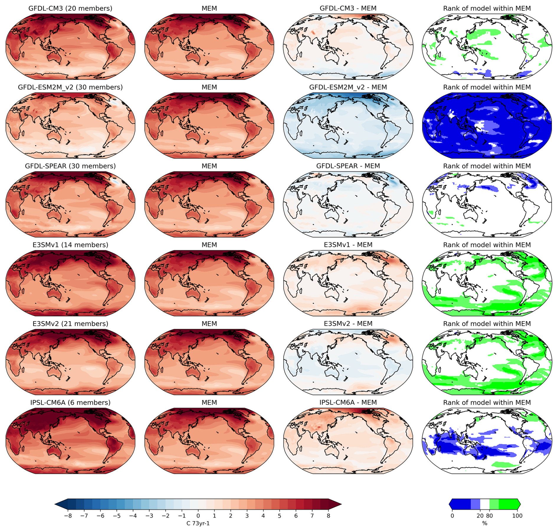
Figure 8 Annual surface air temperature trend from 2027–2099: (left) ensemble mean of Set 2 models, (middle left) MEM, (middle right) difference between the ensemble mean and the MEM, and (right) rank of the model ensemble mean within the MEM. All analysis was completed on RCP8.5 and SSP5-8.5 except for E3SMv1, E3SMv2, CESM2, and UKESM1-0-LL, where SSP3-7.0 was used.

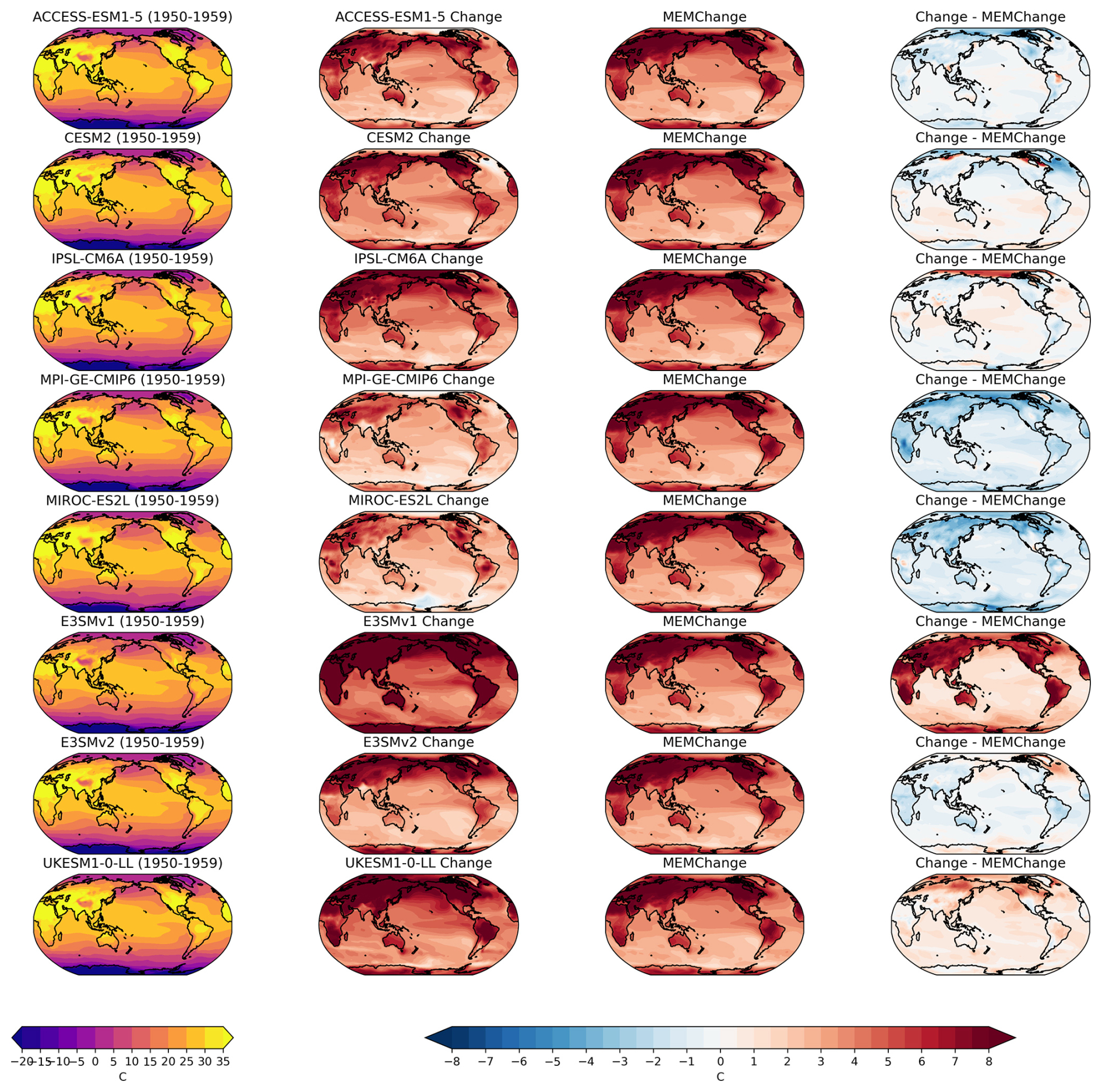
Figure 9 Monthly maximum of the daily maximum temperature (TXx) averaged over June, July, and August in the eight models that have data for the SSP370 future scenario. (Left) individual model ensemble mean for the period 1950–1959, (middle left) the change in 2090–2099 as compared to 1950–1958, (middle right) the change in 2090–2099 as compared to 1950–1959 in the MEM of the eight models shown on the plot, and (right) the change in the single model ensemble mean minus the MEM change.

6 Conclusions

This work has presented two new complementary resources for the study of climate variability and change: the MMLEAv2 and the CVDPv6. Designed for ease of use, these tools provide a broad synthesis of internal and forced contributions to the major modes of climate variability and trends in model LEs in relation to observations, facilitating model evaluation and intercomparison. Here, we have demonstrated some of the insights that can be derived by applying the CVDPv6 to the MMLEAv2. In particular, we have highlighted the following points:

• The MMLEAv2 is an extension of the MMLEA (Deser et al., 2020) with additional models and variables available (18 models and 16 two-dimensional variables).

• The MMLEAv2 is remapped onto a common 2.5 × 2.5° grid for ease of inter-model comparison.

• The MMLEAv2 also provides observed reference datasets on the common 2.5 × 2.5° grid for ease of model-to-observation comparison.

• The CVDPv6 provides a powerful and efficient way to analyse LE output, including the MMLEAv2.

• A preliminary model evaluation has been completed using the CVDPv6 applied to the MMLEAv2 that highlights common model biases, and which models perform well or poorly compared to observations.

• Figs. 1 and 2 of this paper allow the user to determine which climate variables need a LE for fair comparison against observations.

• The CVDPv6 enables the exploration of climate model output and observations, including modes of variability, time series, trends, and spatial maps of key variables.

• Multiple detrending methods can be applied in the CVDPv6, an improvement on previous versions of the package allowing for the efficacy of methods such as quadratic detrending that are typically applied to single realisations (such as observations) to be tested against the removal of the ensemble mean approach (effectively removing the effects of external forcing).

• The CVDPv6 can use any reference dataset (model or observations) and time period for comparison.

• The CVDPv6 output is provided in two complementary ways: Individual Member view and Ensemble Summary view.

• The Ensemble Summary view includes not just spatial plots and time series, but also a rank plot of where the observations sit within the model spread for easy evaluation (i.e. white areas show high model-to-observational agreement).

• The netCDF output is also available from the CVDPv6, which allows uses to create their own additional figures from the diagnostics computed in the package.

• Graphical output is available from the CVDPv6, which can be output as png files for publications and presentation.

• The output is available as an easily navigable HTML format for users to click through (i.e. https://webext.cgd.ucar.edu/Multi-Case/MMLEA_v2/, last access: 15 September 2025).

Additionally, we have demonstrated the utility of LEs for model evaluation. Observations can be considered as one realisation of the world that we live in, meaning that observations are best compared with multiple realisations from a climate model, such as a LE. This is highlighted by the spread of evaluation metrics found across the ensemble. In some cases one ensemble member would evaluate poorly against observations while another would compare favourably. For this reason LEs are important for model evaluation, especially for highly variable quantities. Overall, the MMLEAv2 will allow for exciting new science using LEs and the CVDPv6 is a powerful tool made specifically for the analysis of LEs and their unique characteristics.